galaxies flowing in the oriented saddle frame of the cosmic …mos surveys (malavasi et...
TRANSCRIPT

MNRAS 000, 000–000 (0000) Preprint October 15, 2018 Compiled using MNRAS LATEX style file v3.0
Galaxies flowing in the oriented saddle frame of the cosmic web
K. Kraljic1, C. Pichon1,2,3, Y. Dubois2, S. Codis2, C. Cadiou2, J. Devriendt4,5,M. Musso6, C. Welker7, S. Arnouts8, H. S. Hwang9, C. Laigle4, S. Peirani2,10,A. Slyz4, M. Treyer8 and D. Vibert81 Institute for Astronomy, University of Edinburgh, Royal Observatory, Blackford Hill, Edinburgh, EH9 3HJ, United Kingdom2 CNRS and Sorbonne Universite, UMR 7095, Institut d’Astrophysique de Paris, 98 bis Boulevard Arago, F-75014 Paris, France3 School of Physics, Korea Institute for Advanced Study (KIAS), 85 Hoegiro, Dongdaemun-gu, Seoul, 02455, Republic of Korea4 Sub-department of Astrophysics, University of Oxford, Keble Road, Oxford, OX1 3RH, United Kingdom5 Observatoire de Lyon, UMR 5574, 9 avenue Charles Andre, Saint Genis Laval 69561, France6 East African Institute for Fundamental Research (ICTP-EAIFR), KIST2 Building, Nyarugenge Campus, University of Rwanda, Kigali, Rwanda7 International Centre for Radio Astronomy Research and ASTRO 3D, University of Western Australia, 35 Stirling Highway, Crawley, WA 6009, Australia8 Aix Marseille Univ, CNRS, LAM, Laboratoire d’Astrophysique de Marseille, 38 Rue Frederic Joliot Curie, 13013, Marseille, France9 Quantum Universe Center, Korea Institute for Advanced Study, 85 Hoegiro, Dongdaemun-gu, Seoul 02455, Republic of Korea10 Laboratoire Lagrange, UMR7293, Universite de Nice Sophia Antipolis, CNRS, Observatoire de la Cote d’Azur, 06300 Nice, France
Submitted to MNRAS 2018 August 14
ABSTRACTThe strikingly anisotropic large-scale distribution of matter made of an extended network ofvoids delimited by sheets, themselves segmented by filaments, within which matter flows to-wards compact nodes where they intersect, imprints its geometry on the dynamics of cosmicflows, ultimately shaping the distribution of galaxies and the redshift evolution of their prop-erties. The (filament-type) saddle points of this cosmic web provide a local frame in whichto quantify the induced physical and morphological evolution of galaxies on large scales. Theproperties of virtual galaxies within the HORIZON-AGN simulation are stacked in such a frame.The iso-contours of the galactic number density, mass, specific star formation rate (sSFR),kinematics and age are clearly aligned with the filament axis with steep gradients perpendicu-lar to the filaments. A comparison to a simulation without feedback from active galactic nuclei(AGN) illustrates its impact on quenching star formation of centrals away from the saddles.The redshift evolution of the properties of galaxies and their age distribution are consistentwith the geometry of the bulk flow within that frame. They compare well with expectationsfrom constrained Gaussian random fields and the scaling with the mass of non-linearity, mod-ulo the redshift dependent impact of feedback processes. Physical properties such as sSFR andkinematics seem not to depend only on mean halo mass and density: the residuals trace thegeometry of the saddle, which could point to other environment-sensitive physical processes,such as spin advection, and AGN feedback at high mass.
Key words: galaxies: formation — galaxies: evolution — galaxies: interactions — galaxies:kinematics and dynamics — methods: numerical
1 INTRODUCTION
Galaxies form and evolve within a complex network, the so-called cosmic web (Bond et al. 1996), made of filaments embeddedin sheet-like walls, surrounded by large voids and intersecting atclusters of galaxies (Joeveer et al. 1978). Do the properties of galax-ies, such as their morphology, retain a memory of these large-scalecosmic flows from which they emerge? The importance of interac-tions with the larger scale environment in driving their evolutionhas indeed recently emerged as central tenet of galaxy formationtheory. Galactic masses are highly dependent on their large-scale
surrounding, as elegantly explained by the theory of biased clus-tering (Kaiser 1984; Efstathiou et al. 1988), such that high massobjects preferentially form in over-dense environment near nodes(Bond & Myers 1996; Pogosyan et al. 1996). Conversely, what arethe signatures of this environment away from the nodes of the cos-mic web?
While galaxies grow in mass when forming stars from intensegas inflows at high-redshift, they also acquire spin through tidaltorques and mergers biased by these anisotropic larger scales (e.g.Aubert et al. 2004; Peirani et al. 2004; Navarro et al. 2004; Aragon-Calvo et al. 2007; Codis et al. 2012; Libeskind et al. 2012; Stewartet al. 2013; Trowland et al. 2013; Aragon-Calvo & Yang 2014, for
© 0000 The Authors
arX
iv:1
810.
0521
1v1
[as
tro-
ph.G
A]
11
Oct
201
8
2 K. Kraljic, C. Pichon, Y. Dubois, S. Codis et al.
0 1 2
R [Mpc/h]
−3
−2
−1
0
1
2
3
z[M
pc/h]
[9.00,9.05]
0.2
0.6
1.0
0.0 0.2PDF
0 1 2
R [Mpc/h]
[9.69,9.75]
0.0 0.2PDF
0 1 2
R [Mpc/h]
[10.93,11.99]
0.0 0.2PDF
0
1
2
3
4
5
6
7
8
9
10
11
number
counts
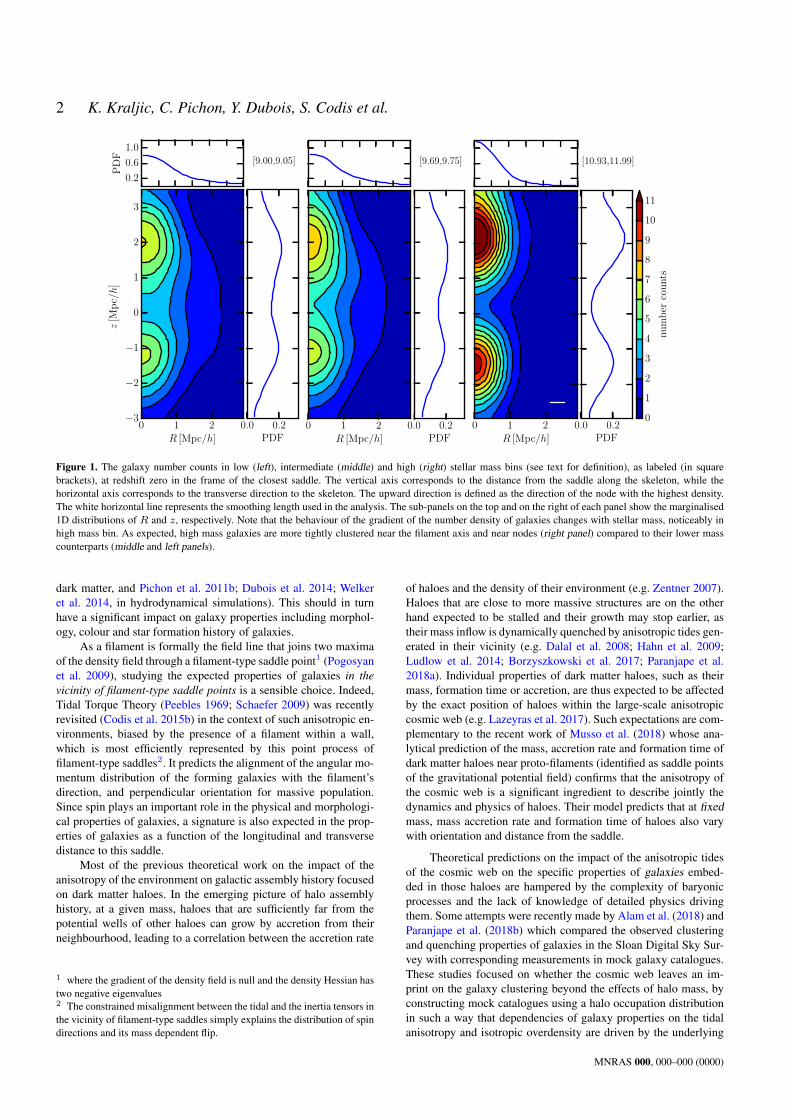
Figure 1. The galaxy number counts in low (left), intermediate (middle) and high (right) stellar mass bins (see text for definition), as labeled (in squarebrackets), at redshift zero in the frame of the closest saddle. The vertical axis corresponds to the distance from the saddle along the skeleton, while thehorizontal axis corresponds to the transverse direction to the skeleton. The upward direction is defined as the direction of the node with the highest density.The white horizontal line represents the smoothing length used in the analysis. The sub-panels on the top and on the right of each panel show the marginalised1D distributions of R and z, respectively. Note that the behaviour of the gradient of the number density of galaxies changes with stellar mass, noticeably inhigh mass bin. As expected, high mass galaxies are more tightly clustered near the filament axis and near nodes (right panel) compared to their lower masscounterparts (middle and left panels).
dark matter, and Pichon et al. 2011b; Dubois et al. 2014; Welkeret al. 2014, in hydrodynamical simulations). This should in turnhave a significant impact on galaxy properties including morphol-ogy, colour and star formation history of galaxies.
As a filament is formally the field line that joins two maximaof the density field through a filament-type saddle point1 (Pogosyanet al. 2009), studying the expected properties of galaxies in thevicinity of filament-type saddle points is a sensible choice. Indeed,Tidal Torque Theory (Peebles 1969; Schaefer 2009) was recentlyrevisited (Codis et al. 2015b) in the context of such anisotropic en-vironments, biased by the presence of a filament within a wall,which is most efficiently represented by this point process offilament-type saddles2. It predicts the alignment of the angular mo-mentum distribution of the forming galaxies with the filament’sdirection, and perpendicular orientation for massive population.Since spin plays an important role in the physical and morphologi-cal properties of galaxies, a signature is also expected in the prop-erties of galaxies as a function of the longitudinal and transversedistance to this saddle.
Most of the previous theoretical work on the impact of theanisotropy of the environment on galactic assembly history focusedon dark matter haloes. In the emerging picture of halo assemblyhistory, at a given mass, haloes that are sufficiently far from thepotential wells of other haloes can grow by accretion from theirneighbourhood, leading to a correlation between the accretion rate
1 where the gradient of the density field is null and the density Hessian hastwo negative eigenvalues2 The constrained misalignment between the tidal and the inertia tensors inthe vicinity of filament-type saddles simply explains the distribution of spindirections and its mass dependent flip.
of haloes and the density of their environment (e.g. Zentner 2007).Haloes that are close to more massive structures are on the otherhand expected to be stalled and their growth may stop earlier, astheir mass inflow is dynamically quenched by anisotropic tides gen-erated in their vicinity (e.g. Dalal et al. 2008; Hahn et al. 2009;Ludlow et al. 2014; Borzyszkowski et al. 2017; Paranjape et al.2018a). Individual properties of dark matter haloes, such as theirmass, formation time or accretion, are thus expected to be affectedby the exact position of haloes within the large-scale anisotropiccosmic web (e.g. Lazeyras et al. 2017). Such expectations are com-plementary to the recent work of Musso et al. (2018) whose ana-lytical prediction of the mass, accretion rate and formation time ofdark matter haloes near proto-filaments (identified as saddle pointsof the gravitational potential field) confirms that the anisotropy ofthe cosmic web is a significant ingredient to describe jointly thedynamics and physics of haloes. Their model predicts that at fixedmass, mass accretion rate and formation time of haloes also varywith orientation and distance from the saddle.
Theoretical predictions on the impact of the anisotropic tidesof the cosmic web on the specific properties of galaxies embed-ded in those haloes are hampered by the complexity of baryonicprocesses and the lack of knowledge of detailed physics drivingthem. Some attempts were recently made by Alam et al. (2018) andParanjape et al. (2018b) which compared the observed clusteringand quenching properties of galaxies in the Sloan Digital Sky Sur-vey with corresponding measurements in mock galaxy catalogues.These studies focused on whether the cosmic web leaves an im-print on the galaxy clustering beyond the effects of halo mass, byconstructing mock catalogues using a halo occupation distributionin such a way that dependencies of galaxy properties on the tidalanisotropy and isotropic overdensity are driven by the underlying
MNRAS 000, 000–000 (0000)

Galaxies in the saddle frame of the cosmic web 3
halo mass function across the cosmic web alone. As such prescrip-tion qualitatively reproduces the main observed trends, and quanti-tatively matches many of the observed results, they concluded thatany additional direct effect of the large-scale tidal field on galaxyformation must be extremely weak.
In this work, the adopted approach is different in that it focusesdirectly on galaxies, their physical properties and redshift evolutionas measured in the large-scale cosmological hydrodynamical simu-lation Horizon-AGN (Dubois et al. 2014, 2016). The main purposeof this paper is to show how the 3D distribution of the physicalproperties of these synthetic galaxies reflects the (tidal) impact ofthe cosmic web on the assembly history of galaxies. It is partly mo-tivated by recent studies carried in the VIPERS, GAMA and COS-MOS surveys (Malavasi et al. 2017; Kraljic et al. 2018; Laigle et al.2018) which showed that the colour and specific star formation rateof galaxies are sensitive to their proximity to the cosmic web atfixed stellar mass and local density. This paper focuses specificallyon the distribution of the galaxy properties stacked in the orientedframe of the filament on large (∼ Mpc) scales. The natural choiceof frame for stacking is defined by filament-type saddle points con-necting two nodes by one filament (in contrast to nodes which aretypically places where the connectivity of filaments is higher).
This paper is organised as follows. Section 2 shortly describesthe simulation and the detection of filaments within. Section 3presents the galactic maps near the saddle, focusing first on thetransverse and longitudinal (azimuthally averaged) maps and thentheir 3D counterparts, while Section 4 shows their redshift evolu-tion. Section 5 relates our finding to the properties of weakly non-Gaussian random fields near saddles. Some observational implica-tions of our work together with the comparison with theoreticalpredictions are discussed in Section 6. Section 7 wraps up.Appendix A explores the robustness of our finding w.r.t. smoothingand choice of filament tracer, Appendix B discusses the redshiftevolution of the geometry of filaments, Appendix C presents com-plementary 2D maps, Appendix D quantifies the position-in-the-saddle frame efficiency of AGN feedback. Appendix E sketchesthe derivation of the theoretical results presented in the main text.Appendix F presents the geometry of the bulk galactic velocity flowin the frame of the saddle. Finally, Appendix G motivates statisti-cally the mediation of mass and density maps over tides. Through-out this paper, by log, we refer to the 10-based logarithm and weloosely use logM as a short term for log(M/M) and logρ forlog(ρ/Mh−2Mpc3).
2 NUMERICAL METHODS
Let us briefly review the main numerical tools used in this workto study the properties of virtual galaxies within the frame of thesaddle.
2.1 Hydrodynamical simulation
The details of the HORIZON-AGN simulation3 can be foundin Dubois et al. (2014), here, only brief description is provided.The simulation is performed with the Adaptive Mesh Refinementcode RAMSES (Teyssier 2002) using a box size of 100h−1 Mpcand adopting a ΛCDM cosmology with total matter density Ωm =0.272, dark energy density ΩΛ = 0.728, baryon density Ωb =
3 see http://www.horizon-simulation.org
0 1 2R [Mpc/h]
−3
−2
−1
0
1
2
3
z[M
pc/h]
[9.00,11.99]
0.250.350.450.55
0.0 0.1 0.2PDF
9.10
9.40
9.50
9.60
9.70
9.80
9.90
9.95
10.00
10.05
10.10
10.15
10.20
10.25
10.30
10.35
10.40
logM
⋆
Figure 2. Mean stellar mass in the frame of the closest saddle for the en-tire galaxy population with masses in the range 109 to 1012M at redshiftzero. The white curves correspond to the contours of the galaxy numbercounts, while the white crosses represent the peaks in galactic number den-sity on axis. More massive galaxies are further away from the saddle (resp.closer to the saddle) than the low mass population in longitudinal (resp.transverse) direction.
0.045, amplitude of the matter power spectrum σ8 = 0.81, Hubbleconstant H0 = 70.4 km s−1 Mpc−1, and ns = 0.967 compatiblewith the WMAP-7 data (Komatsu 2011). The total volume con-tains 10243 dark matter (DM) particles, corresponding to a darkmatter mass resolution of MDM,res = 8× 10⁷ M. The initial gasresolution is Mgas,res = 1 × 10⁷ M. The refinement of the ini-tially coarse 10243 grid down to ∆x = 1 proper kpc is triggeredin a quasi-Lagrangian manner: if the total baryonic mass reaches8 times the initial dark matter mass resolution, or the number ofdark matter particles becomes greater than 8 in a cell, resulting ina typical number of 7 × 10⁹ gas resolution elements (leaf cells) atredshift zero.
The gas heating from a uniform ultraviolet background thattakes place after redshift zreion = 10 is modelled following Haardt& Madau (1996). Gas is allowed to cool down to 104 K throughH and He collisions with a contribution from metals (Sutherland &Dopita 1993). Star formation follows a Schmidt relation in regionsof gas number density above n0 = 0.1 H cm−3: ρ∗ = ε∗ρg/tff ,where ρ∗ is the star formation rate mass density, ρg the gas massdensity, ε∗ = 0.02 the constant star formation efficiency, and tffthe local free-fall time of the gas. Feedback from stellar winds, su-pernovae type Ia and type II are included into the simulation withmass, energy and metal release (see Kaviraj et al. 2017, for furtherdetails).
The HORIZON-AGN simulation includes the formation of blackholes (BHs) that can grow by gas accretion at a Bondi-capped-at-Eddington rate and coalesce when they form a tight enough binary.Energy of BHs can be released in a heating or jet mode (respec-tively “quasar” and “radio” mode) when the accretion rate is re-spectively above and below one per cent of Eddington, with effi-
MNRAS 000, 000–000 (0000)
4 K. Kraljic, C. Pichon, Y. Dubois, S. Codis et al.
ciencies tuned to match the BH-galaxy scaling relations at redshiftzero (see Dubois et al. 2012, for further details).
In order to assess the impact of Active Galactic Nuclei (AGN)feedback on galaxy properties in the frame of saddle, this analy-sis also relies on the HORIZON-NOAGN simulation, which was per-formed with identical initial conditions and sub-grid modelling, butwithout BH formation, thus without AGN feedback (Dubois et al.2016; Peirani et al. 2017).
2.2 Galaxy properties
The identification of galaxies is performed using the most mas-sive sub-node method (Tweed et al. 2009) of the AdaptaHOP halofinder (Aubert et al. 2004) operating on the distribution of star parti-cles with the same parameters as in Dubois et al. (2014). Only struc-tures with a minimum ofNmin = 100 star particles are considered,which typically selects objects with masses larger than 2×10⁸ M.For each redshift output analysed in this paper (0.05 < redshift< 2) catalogues containing up to∼ 350 000 haloes and∼ 180 000galaxies are produced.
For each galaxy, its V/σ, stellar rotation over dispersion, isextracted from the 3D distribution of velocities. This is meant toprovide a kinematic proxy for morphology. The total angular mo-mentum (spin) of stars is first computed in order to define a setof cylindrical spatial coordinates (r, θ, z), with the z-axis orientedalong the spin of galaxy. The velocity of each individual star par-ticle is decomposed into cylindrical components vr , vθ , vz , andthe rotational velocity of a galaxy is V = vθ , the mean of vθof individual stars. The average velocity dispersion of the galaxyσ2 = (σ2
r + σ2θ + σ2
z)/3 is computed using the velocity dispersionof each velocity component σr , σθ , σz .
2.3 Saddle frame identification
In order to quantify the position of galaxies relative to the cos-mic web, a geometric three-dimensional ridge extractor called DIS-PERSE 4 (Sousbie 2011; Sousbie et al. 2011) is run on the full vol-ume gas density distribution over 5123 cells with a 3σ persistencethreshold. This density distribution is smoothed with a Gaussiankernel with smoothing length of 0.8 comoving Mpc/h. The ori-entation and distribution of galaxies can be measured relative tothe direction of the closest filament’s segment. In particular, thecode identifies saddle points along those filaments. This is a costlymethod to identify saddle points, but it provides us with a localpreferred polarity in the frame of the density Hessian (positivelytowards the larger of the two maxima). It was checked that the dis-tributions presented below are relatively insensitive to the choice ofsmoothing length (see Appendix A). It was also checked there thatthese results do not show a strong dependence on the tracer (darkmatter or gas density) used to compute the skeleton.
3 SADDLE STACKS IN 2D AND 3D
With the aim of studying the geometry of the galaxy distributionaround filaments, stacking centred on the saddle points of filamentsis applied. When stacking, two different strategies are explored.
4 The code DISPERSE, which stands for Discrete-Persistent-Structure-Extractor algorithm is publicly available at the following URLhttp://www.iap.fr/users/sousbie/disperse/.
First, stacks are produced centred on the saddle, and physical prop-erties of galaxies are binned as a function of transverse and longi-tudinal distances away from the skeleton. These properties are alsostacked in 3D in the local frame set by the direction of the filamentat the saddle and the 2D inertia tensor in the plane perpendicularto the filament. The former method avoids the flaring induced bythe drift of the curved filaments away from the saddle, only asso-ciate one saddle to each galaxy and stacks azimuthally, while thelatter one allows us to probe the transverse anisotropic geometry offilaments at the saddle.
3.1 Azimuthally averaged stellar mass and number density
Let us start by considering azimuthally averaged 2D maps in theframe defined by the saddle and its steepest ascent direction, andstudy the cross sections of galactic number density and stellar massin the vicinity of the saddle point. In order to infer the variationof galaxy properties beyond its stellar mass, stellar mass will befixed by considering 3 bins, defined as low (9.0 6 logM? 6 9.05),intermediate (9.69 6 logM? 6 9.75) and high (10.93 6 logM? 611.99) stellar mass bins. These bins correspond to the first, middleand last 27-quantiles of the stellar mass distribution of all galaxiesat a given redshift above the stellar mass limit of 109 M. Eachof such constructed stellar mass bin contains ∼ 3500 galaxies. Thesmoothing scale applied to the profiles is 0.4 Mpc/h5.
Figures 1 and 2 show the galactic number counts at low, inter-mediate and high stellar mass, and mean stellar mass for all galax-ies above the stellar mass limit, respectively, at redshift zero in theframe of the saddle. In that frame, the vertical axis correspondsto the distance from the saddle point along the skeleton, upwardstowards the densest node, while the horizontal axis corresponds tothe transverse direction. Note that the length of filaments is not con-stant, however its distribution is quite narrow with median lengthof ∼ 5.5 Mpc/h at redshift zero (see Appendix B, Figure B1). Iso-contours clearly display a dependence both on the radial distancefrom the saddle point and the orientation w.r.t. the filament’s direc-tion. At fixed distance from the saddle point, the number of galaxiesis enhanced in the direction of the filament, i.e. they are more clus-tered in the filaments than in the voids. The gradient of the numberdensity of galaxies is also found to change with stellar mass. Thehigh mass galaxies are more tightly clustered near the filament axisand tend to be further away from saddles along the filament com-pared to their low mass counterparts. Saddle points are, as expected,local minima of both galaxy number counts and stellar mass in thedirection along the filament towards the nodes, and local maxima inthe perpendicular direction. Thus, galaxies in filaments tend to bemore massive than galaxies in voids and within filaments, while thestellar mass of galaxies increases with increasing distance from thesaddle point in the direction toward nodes. This effect is stronger inthe direction perpendicular to the filament, where the relative varia-tion of the mean stellar mass is about a factor of 2 higher comparedto that along the filament.
The mass gradients shown on Figure 2 can be qualitativelyunderstood within peak and excursion set theories (see Section 5and Codis et al. 2015b; Musso et al. 2018).
5 Changing the smoothing scale used to produce the maps to 0.2 and 0.8Mpc/h leads to qualitatively similar conclusions. The smoothing impactsmostly the position of maxima in the transverse direction. At low valuesthese tend to be offset from the filament’s axis because of the smoothing ofthe skeleton itself.
MNRAS 000, 000–000 (0000)

Galaxies in the saddle frame of the cosmic web 5
-2-3
-1
z [Mpc/h] 0
2
43
2
x [Mpc/h]0
-2-3
y [Mpc/h]
-10
12
-2-3
y [Mpc/h]
-1
0
-1
1
2
z [Mpc/h] 0
2
43
2
x [Mpc/h]0
-2-3
Figure 3. 3D structure of the neighbourhood of filaments at redshift zero. The galaxy number counts in the frame of the saddle for masses in the range 109
to 1012M (left) are shown together with two 2D cross sections, longitudinal and transverse, of the filament at the saddle (right). The flattened flaring awayfrom the saddle reflects the co-planarity of filamentary bifurcation within the wall. The top-bottom asymmetry reflects the orientation of the skeleton.
3.2 3D stacks of stellar mass and number density
Let us now investigate the 3D structure of the neighbourhood offilaments by stacking galaxies relative to a 3D-oriented local ref-erence frame, with its origin defined by the position of the saddlepoint and its axes defined as follows: the z-axis corresponds to thedirection of the filament at the saddle, and the x- and y-axes repre-sent major and minor principal axes of the inertia tensor in the planeperpendicular to the filament axis at the saddle point, respectively6.
In order to increase the signal-to-noise ratio, galaxies arestacked by flipping them with respect to the filament axis to pro-duce longitudinal cross sections, and with respect to both principalaxes of the inertia tensor in the case of transverse cross sections.
The 3D distribution of galaxies in such defined frame is shownin Figure 3 (left panel) together with planes representing 2D crosssections, longitudinal and transverse, as used in the analysis (rightpanel). In practice, individual cross sections are obtained by pro-jecting galaxies within ± 1 Mpc/h and ± 0.75 Mpc/h from theplane passing through the saddle point for longitudinal and trans-verse cross sections, respectively. Note the flaring near the nodeswhich arises because the typical saddle is flattened (the two neg-ative eigenvalues of the Hessian differ, while the correspondingeigenvectors are aligned when stacking), and the Hessian remainscorrelated away from the saddle. Correspondingly, the skeleton bi-furcates within that plane (Pogosyan et al. 2009; Codis et al. 2018).The top-bottom asymmetry reflects the fact that higher density con-
6 In practice, the 2D inertia tensor is computed by considering galaxieswithin ± 1 (Mpc/h) around the saddle point and projected into the planeperpendicular to the filament and passing through the saddle. Note thatchanging the volume of the considered region within a factor of a few doesnot have a strong impact on orientation.
tours are drawn near the more prominent peak (which is traced bythe orientation of the skeleton).
As in the case of azimuthally averaged cross sections, threestellar mass bins are defined as low (9.0 6 logM? 6 9.05), in-termediate (9.7 6 logM? 6 9.77) and high (10.96 6 logM? 611.99) stellar mass bins, containing ∼ 10 000 and ∼ 1000 galax-ies, for longitudinal and transverse cross sections, respectively. Theupward direction along z-axis corresponds to the direction of thenode with highest density, and the smoothing scale applied to theprofiles is 0.4 Mpc/h, as previously.
The cross sections of galactic number counts, stellar mass,specific star formation rate sSFR = SFR/M∗, where SFR is com-puted over a timescale of 50 Myr, V/σ and age will be studied inthe vicinity of the saddle. Figures 4 and 5 show the galaxy numbercounts in three different stellar mass bins, and mean stellar massfor all galaxies above the stellar mass limit, respectively, at red-shift zero in the longitudinal (top panels) and transverse (bottompanels) planes in the frame of the saddle. Once again, iso-contoursclearly depend on both the radial distance from the saddle and theorientation w.r.t. the filament’s direction. Galaxies are found to bemore clustered in filaments than in voids at all masses, i.e. at fixeddistance from the saddle point, the number of galaxies is enhancedin the direction of the filament. What changes with stellar mass isthe behaviour of the gradients with the most massive galaxies be-ing more tightly clustered near the filament axis compared to theirlower mass counterparts. As in the case of azimuthally averagedcross sections, mass gradients seen in Figure 5 (left panels) canbe also understood in the context of constrained random field andexcursion set theory, as discussed in Section 5.
Interestingly, the distribution of most massive galaxies aroundthe saddle points in the transverse direction is axisymmetric up tothe distance of ∼ 1 Mpc/h, while the iso-contours of lower mass
MNRAS 000, 000–000 (0000)

6 K. Kraljic, C. Pichon, Y. Dubois, S. Codis et al.
−3
−2
−1
0
1
2
3
4
z[M
pc/h]
[9.00,9.05]
0.2
0.7
1.2
0.12 0.28
[9.70,9.77]
0.12 0.28
[10.96,11.99]
0.12 0.280.00.61.21.82.43.03.64.24.85.46.06.67.28.08.69.211.713.5
number
counts
−2 −1 0 1 2y [Mpc/h]
−1
0
1
x[M
pc/h]
0.4
1.2
0.4 1.2PDF
−2 −1 0 1 2y [Mpc/h]
0.4 1.2PDF
−2 −1 0 1 2y [Mpc/h]
0.4 1.2PDF
0.000.350.600.901.401.902.402.903.403.904.404.905.506.80
number
counts
Figure 4. The galaxy number counts at redshift zero in the frame of the saddle for low (left), intermediate (middle) and high (right) stellar mass bins (see textfor definition), as labeled (in square brackets), in the longitudinal (top) and transverse (bottom) planes at the saddle. The vertical axis on top panels correspondsto the direction of the skeleton at the saddle (upwards toward the node with the highest density), while the horizontal axis corresponds to the major principalaxis in the transverse direction. The sub-panels on the top and on the right of each panel show the marginalised 1D distributions along respective axes. Thewhite dashed contours represent the galaxy number counts with the horizontal axis corresponding to the minor principal axis in the transverse direction at thesaddle. The black crosses represent the peaks in galactic density on axis and the white horizontal line represents the smoothing length used in the analysis.The projection is carried over ±1 Mpc/h for the longitudinal slice and ±0.75 Mpc/h away from the saddles transversally. The strength of the gradient of thegalaxy number density changes with stellar mass. As expected, the high mass galaxies are more tightly clustered near the filament axis and near nodes (rightpanel) compared to their low mass counterparts (left and middle panels).
galaxies are more flattened (in the direction of x-axis correspond-ing to the major axis of the inertia tensor in the transverse crosssection) and extended to larger distances from the saddle. This be-haviour is a manifestation of the mass dependence of galaxy’s con-nectivity: higher mass galaxies in denser environments are expectedto be fed by numerous filaments while lower mass galaxies are typ-ically embedded in a single filament (Codis et al. 2018).
3.3 Longitudinal and transverse sSFR cross sections
Let us now focus on specific star formation rates. Figure 6 (toprow) shows the mean stellar mass-weighted sSFR at redshift zeroin HORIZON-AGN. Iso-contours display qualitatively similar be-haviour in all stellar mass bins in the direction perpendicular tothe filament, for which the saddle point represents the maximumof sSFR. In the direction along the filament, the behaviour is morecomplex: at high stellar mass sSFR increases with increasing dis-tance from the saddle towards the nodes, but while the maximumof sSFR overlaps with the position of the low density node, it islocated closer to the saddle in the direction of the densest node,as will be discussed below. The sSFR then decreases in this direc-
tion in the vicinity of the node and beyond. With decreasing stellarmass, the maximum of sSFR moves closer to the saddle point, untilit overlaps with the saddle point for lowest stellar mass bin.
A general trend of decreasing sSFR with increasing stellarmass is clearly recovered, with most massive galaxies having theirsSFR substantially reduced in particular in the vicinity of the dens-est node, where the average sSFR value can be up to 10-times lowercompared to their low mass counterparts. Indeed AGN feedbackis an important ingredient for the formation of the more massivegalaxies, suppressing star formation so as to reproduce the observedhigh-end of the galaxy luminosity function. By comparing the iso-contours of mean stellar mass-weighted sSFR in HORIZON-AGNand HORIZON-NOAGN (bottom row of Figure 6), the two main spe-cific consequences of AGN feedback can be identified. First, andnot surprisingly, when AGN feedback operates, the overall sSFR isreduced, mostly in the high stellar mass bin (the mean sSFR in thehighest stellar mass bin changes by a factor of ∼ 3, while in thelowest stellar mass bin, it remains ∼ 1.15). Secondly, AGN feed-back modifies the shape of sSFR iso-contours. This effect is most
MNRAS 000, 000–000 (0000)
Galaxies in the saddle frame of the cosmic web 7
−3
−2
−1
0
1
2
3
4
z[M
pc/h]
[9.00,11.99]
0.400.460.52
0.10 0.189.59
9.65
9.70
9.80
9.85
9.90
9.94
10.00
10.05
10.10
10.15
10.20
10.25
10.30
10.35
10.41
logM
⋆
−2 −1 0 1 2y [Mpc/h]
−1
0
1
x[M
pc/h]
0.420.480.54
0.45 0.62PDF
9.499.659.759.859.959.9910.0210.0510.0710.0910.15
logM
⋆
−3
−2
−1
0
1
2
3
4
z[M
pc/h]
[9.00,11.99]
0.35
0.45
0.55
0.1 0.211.0011.2011.3011.4011.5011.6011.7011.8011.9012.0012.1012.2012.3012.4012.5012.5812.70
logM
h−2 −1 0 1 2
y [Mpc/h]
−1
0
1
x[M
pc/h]
0.40
0.55
0.70
0.45 0.80PDF
11.0011.1011.2011.3011.4011.5011.6011.7011.8011.9012.10
logM
h
−3
−2
−1
0
1
2
3
4
z[M
pc/h]
[9.00,11.99]
0.35
0.45
0.55
0.1 0.211.50
11.70
11.90
12.00
12.20
12.40
12.60
12.80
13.00
13.20
13.40
13.60
logM
main
h
−2 −1 0 1 2y [Mpc/h]
−1
0
1
x[M
pc/h]
0.40
0.55
0.65
0.45 0.78PDF
11.30
11.40
11.50
11.60
11.80
12.00
12.20
12.40
12.60
logM
main
h
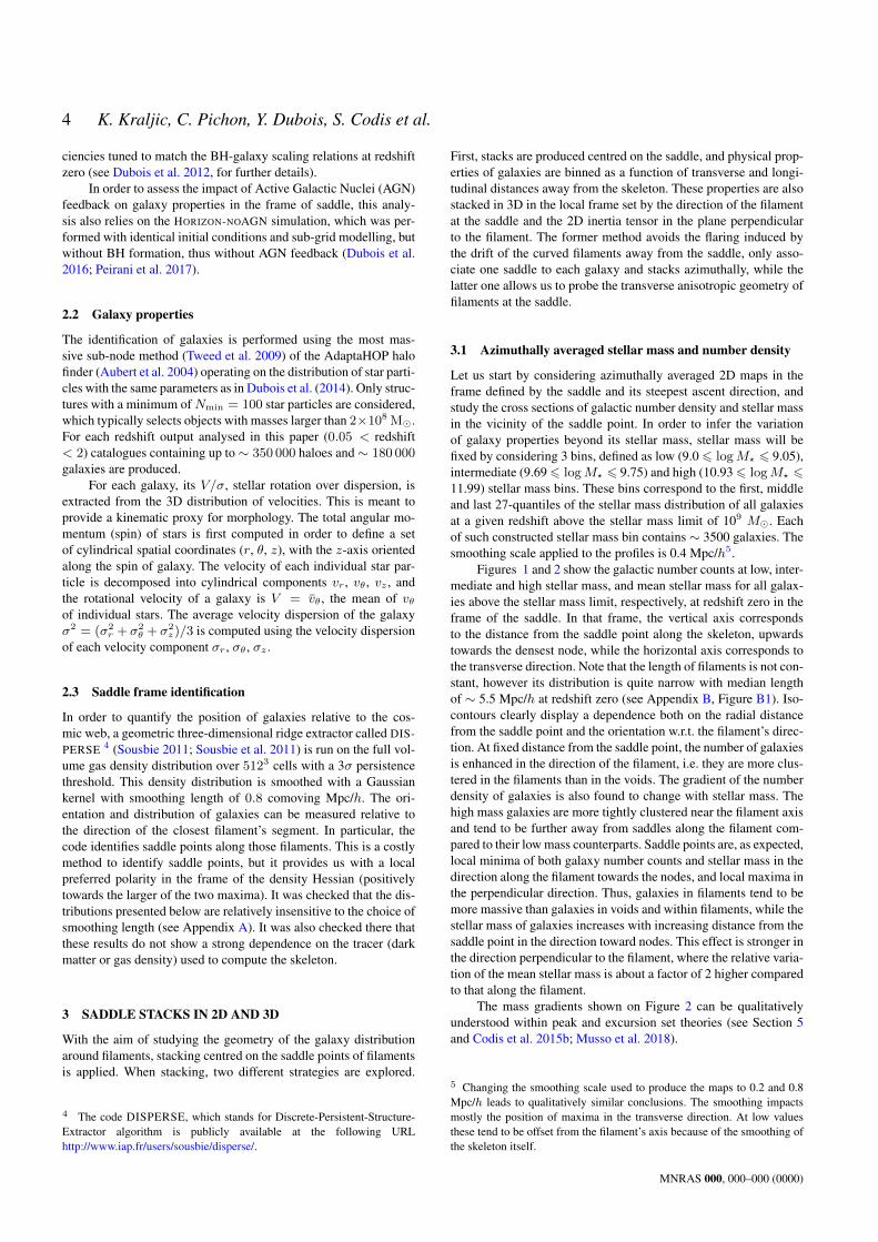
Figure 5. Mean galaxy stellar mass (left), sub-halo mass (middle) and host halo mass (right) in the frame of the saddle for masses in the range 109 to 1012Mat redshift zero, in the longitudinal (top panels) and transverse (bottom panels) planes at the saddle. The vertical axis corresponds to the direction of the skeletonat the saddle (upwards toward the node with the highest density), while the horizontal axis corresponds to the major principal axis in the transverse direction.The white contours correspond to the galaxy number counts with the horizontal axis corresponding to the major principal axis in the transverse direction at thesaddle. The white cross represent the peak in galactic density on axis. More massive galaxies are further away from the saddle than the low mass population inthe longitudinal direction, while they are closer to the saddle transversally. As expected, more massive galaxies are also residing in more massive halos. Notein particular that the iso-contours of stellar mass are very similar to those of sub-halo mass, while the iso-contours of host halo mass, the shape of which differfrom the two others, show much more resemblance to the iso-contours of density (as discussed in Section 6). The peak of maximum mass is further away fromthe saddle than the counts.
prominent amongst most massive galaxies7 in the vicinity of thedensest node that represents the maximum of the sSFR in the di-rection along the filament from the saddle when AGN feedback isabsent. A similar effect is seen at low and intermediate stellar mass,albeit less pronounced. Overall, the reduced star formation activ-ity of galaxies due to AGN feedback in the densest environmenttranslates into an offset of the maximum of the mean stellar mass-weighted sSFR away from the node. This clearly demonstrates theimportance of the AGN feedback and its ability not only to reducethe star formation activity of individual objects, but also to mod-ify their distribution on larger scales in the vicinity of high densityregions such as nodes, corresponding to galaxy groups and clus-ters, consistently with our findings of AGN feedback being mostefficient near nodes at high stellar mass (see Appendix D).
7 Note that the highest stellar mass bin is not identical in the two simula-tions. This is due to the difference in the stellar mass distributions, such thatat high stellar mass end, there are more galaxies in HORIZON-NOAGN thanin HORIZON-AGN that also tend to be more massive (see also Beckmannet al. 2017). However, considering the same stellar mass bins does not im-pact our results. Another difference is in the halo-to-stellar mass relation,especially at the high mass end. It was checked that the medians of halomasses in the highest stellar mass bin considered in this work are compara-ble in both simulations.
3.4 Centrals and satellite differential counts
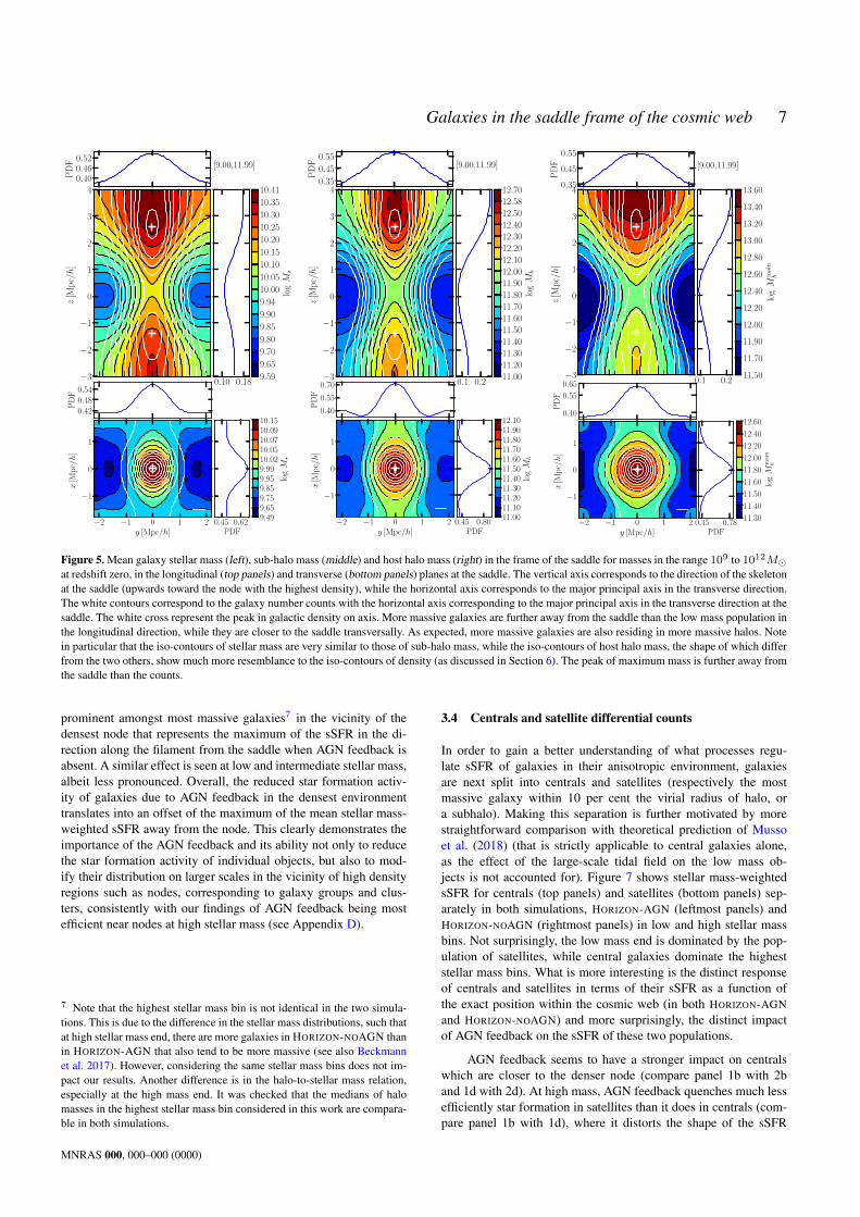
In order to gain a better understanding of what processes regu-late sSFR of galaxies in their anisotropic environment, galaxiesare next split into centrals and satellites (respectively the mostmassive galaxy within 10 per cent the virial radius of halo, ora subhalo). Making this separation is further motivated by morestraightforward comparison with theoretical prediction of Mussoet al. (2018) (that is strictly applicable to central galaxies alone,as the effect of the large-scale tidal field on the low mass ob-jects is not accounted for). Figure 7 shows stellar mass-weightedsSFR for centrals (top panels) and satellites (bottom panels) sep-arately in both simulations, HORIZON-AGN (leftmost panels) andHORIZON-NOAGN (rightmost panels) in low and high stellar massbins. Not surprisingly, the low mass end is dominated by the pop-ulation of satellites, while central galaxies dominate the higheststellar mass bins. What is more interesting is the distinct responseof centrals and satellites in terms of their sSFR as a function ofthe exact position within the cosmic web (in both HORIZON-AGNand HORIZON-NOAGN) and more surprisingly, the distinct impactof AGN feedback on the sSFR of these two populations.
AGN feedback seems to have a stronger impact on centralswhich are closer to the denser node (compare panel 1b with 2band 1d with 2d). At high mass, AGN feedback quenches much lessefficiently star formation in satellites than it does in centrals (com-pare panel 1b with 1d), where it distorts the shape of the sSFR
MNRAS 000, 000–000 (0000)

8 K. Kraljic, C. Pichon, Y. Dubois, S. Codis et al.
−3
−2
−1
0
1
2
3
4z[M
pc/h]
9.00≤ logM⋆ ≤ 9.05
−2 −1 0 1 2y [Mpc/h]
−1
0
1
x[M
pc/h]
9.70≤ logM⋆ ≤ 9.77
−2 −1 0 1 2y [Mpc/h]
10.96≤ logM⋆ ≤ 11.99
0.400.951.151.251.301.401.451.482.003.003.253.604.004.304.705.005.205.506.006.236.35
sSFR/10−
11[yr−
1]
−2 −1 0 1 2y [Mpc/h]
0.000.280.891.201.502.002.503.013.453.804.505.206.006.708.00
sSFR/10−
11[yr−
1]
noAGN
−3
−2
−1
0
1
2
3
4
z[M
pc/h]
9.00≤ logM⋆ ≤ 9.05
−2 −1 0 1 2y [Mpc/h]
−1
0
1
x[M
pc/h]
9.74≤ logM⋆ ≤ 9.81
−2 −1 0 1 2y [Mpc/h]
11.26≤ logM⋆ ≤ 12.00
0.400.951.151.251.301.401.451.482.003.003.253.604.004.304.705.005.205.506.006.236.35
sSFR/10−
11[yr−
1]
−2 −1 0 1 2y [Mpc/h]
0.000.280.891.201.502.002.503.013.453.804.505.206.006.708.00
sSFR/10−
11[yr−
1]
noAGN
Figure 6. Mass-weighted sSFR in the frame of the saddle at redshift 0 for low (left), intermediate (middle) and high (right) stellar mass bins, as labeled,in the longitudinal and transverse planes at the saddle, in HORIZON-AGN (topmost panels) and HORIZON-NOAGN (bottommost panels). The vertical axiscorresponds to the direction of the skeleton at the saddle (upwards toward the node with the highest density), while the horizontal axis corresponds to themajor principal axis in the transverse direction at the saddle. The white contours and the white crosses correspond to the galaxy number counts and the peakin galactic density on axis, respectively. The saddle represents maximum of sSFR in transverse direction at all masses and regardless of the presence of theAGN feedback. What does change is the star formation activity in particular of the most massive galaxies, where AGN feedback substantially reduces thevalues of sSFR. Moreover, note that at high mass end, the sSFR iso-contours are modified by AGN feedback in the vicinity of the densest node, such thatin the longitudinal direction away from the saddle, the maximum of sSFR is off-set from the densest peak. Overall, the sSFR iso-contours display a stellarmass dependence in the longitudinal direction in that at low mass (resp. high mass) sSFR is maximum (resp. minimum) at the saddle and it decreases (resp.increases) in the direction towards the nodes.
MNRAS 000, 000–000 (0000)
Galaxies in the saddle frame of the cosmic web 9
−3
−2
−1
0
1
2
3
4
z[M
pc/h]
9.00≤ logM⋆ ≤ 9.06 10.96≤ logM⋆ ≤ 11.99
0.200.600.951.151.251.401.501.651.802.002.503.003.303.604.004.304.605.005.205.505.605.705.906.00
sSFR/10−
11[yr−
1]
centrals
1a 1b
AGN
−2 −1 0 1 2y [Mpc/h]
−3
−2
−1
0
1
2
3
4
z[M
pc/h]
−2 −1 0 1 2y [Mpc/h]
0.200.600.951.151.251.401.501.651.802.002.503.003.303.604.004.304.605.005.205.505.605.705.906.00
sSFR/10−
11[yr−
1]
satellites
1c 1d
−3
−2
−1
0
1
2
3
4
z[M
pc/h]
9.00≤ logM⋆ ≤ 9.06 11.27≤ logM⋆ ≤ 12.00
0.200.600.951.151.251.401.501.651.802.002.503.003.303.604.004.304.605.005.205.505.605.705.906.00
sSFR/10−
11[yr−
1]
centrals
2a 2b
noAGN
−2 −1 0 1 2y [Mpc/h]
−3
−2
−1
0
1
2
3
4
z[M
pc/h]
−2 −1 0 1 2y [Mpc/h]
0.200.600.951.151.251.401.501.651.802.002.503.003.303.604.004.304.605.005.205.505.605.705.906.00
sSFR/10−
11[yr−
1]
satellites
2c 2d
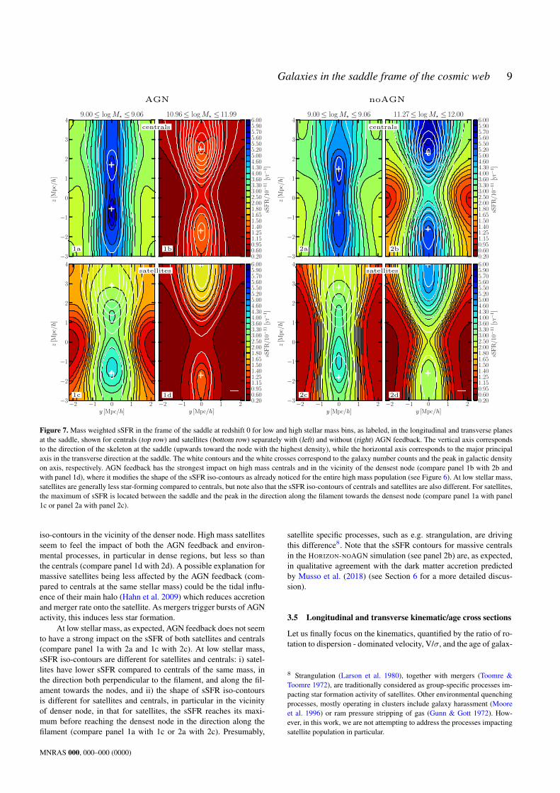
Figure 7. Mass weighted sSFR in the frame of the saddle at redshift 0 for low and high stellar mass bins, as labeled, in the longitudinal and transverse planesat the saddle, shown for centrals (top row) and satellites (bottom row) separately with (left) and without (right) AGN feedback. The vertical axis correspondsto the direction of the skeleton at the saddle (upwards toward the node with the highest density), while the horizontal axis corresponds to the major principalaxis in the transverse direction at the saddle. The white contours and the white crosses correspond to the galaxy number counts and the peak in galactic densityon axis, respectively. AGN feedback has the strongest impact on high mass centrals and in the vicinity of the densest node (compare panel 1b with 2b andwith panel 1d), where it modifies the shape of the sSFR iso-contours as already noticed for the entire high mass population (see Figure 6). At low stellar mass,satellites are generally less star-forming compared to centrals, but note also that the sSFR iso-contours of centrals and satellites are also different. For satellites,the maximum of sSFR is located between the saddle and the peak in the direction along the filament towards the densest node (compare panel 1a with panel1c or panel 2a with panel 2c).
iso-contours in the vicinity of the denser node. High mass satellitesseem to feel the impact of both the AGN feedback and environ-mental processes, in particular in dense regions, but less so thanthe centrals (compare panel 1d with 2d). A possible explanation formassive satellites being less affected by the AGN feedback (com-pared to centrals at the same stellar mass) could be the tidal influ-ence of their main halo (Hahn et al. 2009) which reduces accretionand merger rate onto the satellite. As mergers trigger bursts of AGNactivity, this induces less star formation.
At low stellar mass, as expected, AGN feedback does not seemto have a strong impact on the sSFR of both satellites and centrals(compare panel 1a with 2a and 1c with 2c). At low stellar mass,sSFR iso-contours are different for satellites and centrals: i) satel-lites have lower sSFR compared to centrals of the same mass, inthe direction both perpendicular to the filament, and along the fil-ament towards the nodes, and ii) the shape of sSFR iso-contoursis different for satellites and centrals, in particular in the vicinityof denser node, in that for satellites, the sSFR reaches its maxi-mum before reaching the densest node in the direction along thefilament (compare panel 1a with 1c or 2a with 2c). Presumably,
satellite specific processes, such as e.g. strangulation, are drivingthis difference8. Note that the sSFR contours for massive centralsin the HORIZON-NOAGN simulation (see panel 2b) are, as expected,in qualitative agreement with the dark matter accretion predictedby Musso et al. (2018) (see Section 6 for a more detailed discus-sion).
3.5 Longitudinal and transverse kinematic/age cross sections
Let us finally focus on the kinematics, quantified by the ratio of ro-tation to dispersion - dominated velocity, V/σ, and the age of galax-
8 Strangulation (Larson et al. 1980), together with mergers (Toomre &Toomre 1972), are traditionally considered as group-specific processes im-pacting star formation activity of satellites. Other environmental quenchingprocesses, mostly operating in clusters include galaxy harassment (Mooreet al. 1996) or ram pressure stripping of gas (Gunn & Gott 1972). How-ever, in this work, we are not attempting to address the processes impactingsatellite population in particular.
MNRAS 000, 000–000 (0000)
10 K. Kraljic, C. Pichon, Y. Dubois, S. Codis et al.
−3
−2
−1
0
1
2
3
4z[M
pc/h]
9.00≤ logM⋆ ≤ 9.05
−2 −1 0 1 2y [Mpc/h]
−1
0
1
x[M
pc/h]
9.70≤ logM⋆ ≤ 9.77
−2 −1 0 1 2y [Mpc/h]
10.96≤ logM⋆ ≤ 11.99
0.00
0.05
0.07
0.09
0.11
0.12
0.13
0.14
0.15
0.16
0.19
0.22
0.23
0.24
0.25
0.26
0.27
0.28
V/σ
−2 −1 0 1 2y [Mpc/h]
0.000.070.090.100.120.140.160.190.220.230.240.250.260.270.28
V/σ
−3
−2
−1
0
1
2
3
4
z[M
pc/h]
9.00≤ logM⋆ ≤ 9.05
−2 −1 0 1 2y [Mpc/h]
−1
0
1
x[M
pc/h]
9.70≤ logM⋆ ≤ 9.77
−2 −1 0 1 2y [Mpc/h]
10.96≤ logM⋆ ≤ 11.99
2.00
3.00
4.00
4.50
5.00
5.30
5.70
6.00
6.30
6.70
7.00
7.30
7.70
8.00
8.50
age[Gyr]
−2 −1 0 1 2y [Mpc/h]
0.501.001.502.002.503.003.504.004.505.005.505.806.106.406.60
age[Gyr]
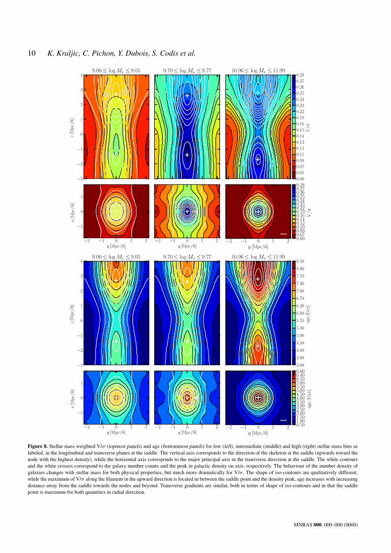
Figure 8. Stellar mass weighted V/σ (topmost panels) and age (bottommost panels) for low (left), intermediate (middle) and high (right) stellar mass bins aslabeled, in the longitudinal and transverse planes at the saddle. The vertical axis corresponds to the direction of the skeleton at the saddle (upwards toward thenode with the highest density), while the horizontal axis corresponds to the major principal axis in the transverse direction at the saddle. The white contoursand the white crosses correspond to the galaxy number counts and the peak in galactic density on axis, respectively. The behaviour of the number density ofgalaxies changes with stellar mass for both physical properties, but much more dramatically for V/σ. The shape of iso-contours are qualitatively different,while the maximum of V/σ along the filament in the upward direction is located in between the saddle point and the density peak, age increases with increasingdistance away from the saddle towards the nodes and beyond. Transverse gradients are similar, both in terms of shape of iso-contours and in that the saddlepoint is maximum for both quantities in radial direction.
MNRAS 000, 000–000 (0000)

Galaxies in the saddle frame of the cosmic web 11
ies in the frame of the saddle. The observational proxies of thesequantities would be morphology and colour, respectively. HigherV/σ typically characterises disc dominated morphologies, whilelower V/σ indicates the presence of a substantial bulge component.The age of galaxies corresponds to the mean ages that are given bythe mass-weighted age of star particles belonging to each galaxy.Figure 8 shows iso-contours of V/σ (top panels) and age (bottompanels) as a function of stellar mass at redshift zero. Again, thecontours exhibit both radial and angular gradients w.r.t. the sad-dle point. At all stellar mass bins, galaxies tend to have higherV/σ in the vicinity of the saddle point that decreases in the or-thogonal direction away from the saddle, while in the directionalong the filament towards the nodes it first increases, reaches itsmaximum before getting to the densest node and decreases after-wards. This effect is strongest for highest mass galaxies. In termsof quantitative comparison of V/σ at different stellar mass, galaxiesin the lowest stellar mass bin have the lowest V/σ, while interme-diate mass galaxies show the largest V/σ values. V/σ of the mostmassive galaxies is lower compared to intermediate stellar masses,but higher than at lowest stellar mass end. This can be explainedby the presence of few massive disc dominated galaxies presentin the HORIZON-AGN simulation and higher fraction of ellipticalsat low mass end compared to observations. Indeed, as shown inDubois et al. (2016), the maximum probability of finding discs inHORIZON-AGN is in the stellar mass range of 1010 − 1011M.
Similarly, age gradients display clear radial and angular de-pendence w.r.t. the saddle point at all stellar mass bins, however,with qualitatively different behaviour. In the transverse direction,saddle point is still maximum of the age at all stellar mass, whilein the direction along the filament away from the saddle, age in-creases all the way beyond the node. Interestingly, in this aspect,age gradients are similar to stellar mass gradients with the oldestand most massive galaxies being located closer to the node in thedirection of the filament, and in the vicinity of the filament in theorthogonal direction. This is consistent with the redshift evolutionof the stacks as discussed now.
4 REDSHIFT EVOLUTION
Let us now examine the evolution of galaxy properties with red-shift. When comparing different epochs one may either considerthe fate of a given set of galaxies, or quantify the cosmic evolutionof the galactic population as a whole.
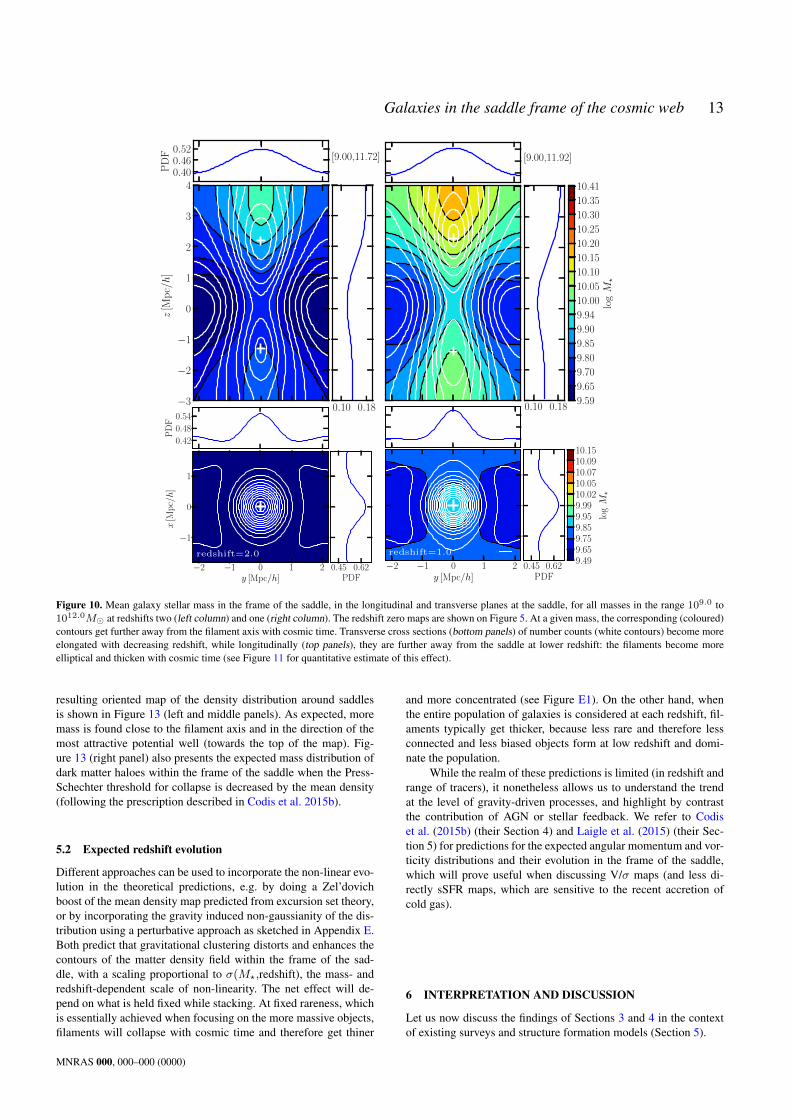
Figure 9 shows galaxy number counts in low (left column),intermediate (middle column) and high (right column) stellar massbins at redshifts two (topmost rows) and one (bottommost rows)9,while Figure 10 shows the mean stellar mass of the entire popu-lation above the mass limit at these redshifts, as indicated10. Thecorresponding redshift zero maps are shown on Figures 4 and 5,respectively.
At each redshift, more massive galaxies are more tightly clus-tered in the filaments than in the voids, and near the nodes thannear the saddles. Part of this redshift evolution is simply due to themass evolution of objects. In other words, one could fix the level
9 The skeleton and stellar mass bins are constructed as for redshift zero, seeSections 2.3 and 3.2, respectively. Consequently, the stellar mass bins arenot identical at different redshifts, but they still contain comparable numberof galaxies.10 Note that these cross-sections are in qualitative agreement with az-imuthally averaged counterparts (see Appendix C).
of non-linearity by considering mass bins that evolve with redshiftfollowing the non-linear mass for instance and then consider theresidual redshift evolution. This procedure would allow to focus onthe same class of objects across redshifts.
On Figure 9, one can follow the progenitors of a given classof objects by fixing the level of non-linearity which is equivalentto move approximatively along the diagonal (by adding Figure 4),i.e. to focus on less massive objects at high redshift. As galaxiesgrow in mass, i.e. as non-linear gravitational clustering proceeds(the local dynamical clocks being set by inverse square root of thelocal density), they also become more concentrated towards the fil-aments and nodes (see Appendix E2). For instance, comparing thebottom right transverse cross-section at redshift one and zero (fromFigure 4), the vicinity of the saddle is less populated by massiveobjects as these have drifted towards the nodes. This redshift evo-lution is consistent with the global flow of galaxies first towardsthe filaments and then along them (as quantified kinematically inAppendix F), and with the fact that galaxies accumulate mass withcosmic time.
For a population as a whole, in the close vicinity of the saddle,the breadth of the filament broadens with cosmic time as shownin Figure 11, comparing the filament’s thickness for all galaxiesabove the stellar mass limit at redshifts two and zero. Specifically,the full width at half maximum (FWHM) of the transverse galaxynumber counts profiles was computed at different positions alongthe filament’s direction. As argued in the next section, the measuredincrease of the filament’s width with cosmic time is consistent withthe theoretical expectations.
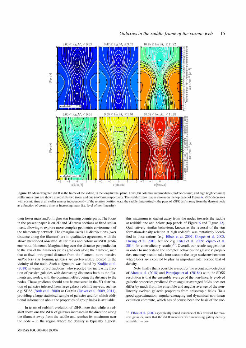
Finally, Figure 12 shows the redshift evolution of stellar mass-weighted sSFR. Again, it is interesting to note that the global sSFRtraces the level of non-linearity of the collapse of structures: at highredshift, low mass population (top left panel) has the highest sSFR,whereas the high mass low redshift population (bottom right panel)is the most quenched. This is also reflected in the position of max-imum of sSFR, which drifts with cosmic time i.e. with the level ofnon-linearity of the field. The peak of sSFR seems to occur furtherfrom the denser nodes towards the saddle as a function of cosmictime. Hence, for the sSFR at least two processes compete: advec-tion with the main flow and star formation activity which is im-pacted by the proximity to AGNs and the local dynamical timescale(but see Section 6.6 below).
5 THEORETICAL PREDICTIONS
Let us briefly present the theoretical framework which will allowus to interpret the measurements presented in Sections 3 and 4.This will involve predictions for dark matter and halo density crosssections in the frame of the saddle, and their expected non-linearevolution with cosmic time.
5.1 Constrained random fields
For Gaussian cosmological initial conditions, peak theory (Bardeenet al. 1986) can be adapted to predict the mean (total) matter densitymaps around saddles. Appendix E derives this mean initial matterdistribution marginalised to the constraint of a saddle point of ar-bitrary geometry (height and curvatures) when the direction of thelargest (positive) eigenvalue of the Hessian, i.e the direction of thefilament, is fixed together with its orientation. This last requirementis achieved by imposing that the coordinate of the gradient of thegravitational potential along the filament is always negative. The
MNRAS 000, 000–000 (0000)

12 K. Kraljic, C. Pichon, Y. Dubois, S. Codis et al.
−3
−2
−1
0
1
2
3
4
z[M
pc/h]
[9.00,9.03]
0.2
0.7
1.2
0.12 0.28
[9.47,9.52]
0.12 0.28
[10.45,11.72]
0.12 0.280.00.61.21.82.43.03.64.24.85.46.06.67.28.08.69.211.713.5
number
counts
−2 −1 0 1 2y [Mpc/h]
−1
0
1
x[M
pc/h]
0.4
1.2
0.4 1.2PDF
−2 −1 0 1 2y [Mpc/h]
0.4 1.2PDF
−2 −1 0 1 2y [Mpc/h]
0.4 1.2PDF
0.000.350.600.901.401.902.402.903.403.904.404.905.506.80
number
counts
redshift=2.0
−3
−2
−1
0
1
2
3
4
z[M
pc/h]
[9.00,9.04]
0.2
0.7
1.2
0.12 0.28
[9.58,9.64]
0.12 0.28
[10.68,11.92]
0.12 0.280.00.61.21.82.43.03.64.24.85.46.06.67.28.08.69.211.713.5
number
counts
−2 −1 0 1 2y [Mpc/h]
−1
0
1
x[M
pc/h]
0.4
1.2
0.4 1.2PDF
−2 −1 0 1 2y [Mpc/h]
0.4 1.2PDF
−2 −1 0 1 2y [Mpc/h]
0.4 1.2PDF
0.000.350.600.901.401.902.402.903.403.904.404.905.506.80
number
counts
redshift=1.0
Figure 9. Redshift evolution of the galaxy number counts in the frame of the saddle, in the longitudinal and transverse planes at the saddle. Low (left column),intermediate (middle column) and high (right column) stellar mass bins are shown at redshifts 2 (top-most panels) and 1 (bottom-most panels), respectively.The white dashed contours represent the galaxy number counts with the horizontal axis corresponding to the minor principal axis in the transverse direction atthe saddle. The corresponding redshift zero maps are shown on Figure 4. High mass galaxies are more clustered near the filaments and nodes at all redshiftsconsidered compared to their lower mass counterparts. Note that as galaxies grow in mass with time, they follow the global flow of matter, reflected by theincreased distance between the saddle point and two respective nodes at lower redshift.
MNRAS 000, 000–000 (0000)
Galaxies in the saddle frame of the cosmic web 13
−3
−2
−1
0
1
2
3
4
z[M
pc/h]
[9.00,11.72]
0.400.460.52
0.10 0.18
−2 −1 0 1 2y [Mpc/h]
−1
0
1
x[M
pc/h]
0.42
0.48
0.54
0.45 0.62PDF
redshift=2.0
[9.00,11.92]
0.10 0.189.59
9.65
9.70
9.80
9.85
9.90
9.94
10.00
10.05
10.10
10.15
10.20
10.25
10.30
10.35
10.41
logM
⋆
−2 −1 0 1 2y [Mpc/h]
0.45 0.62PDF
9.499.659.759.859.959.9910.0210.0510.0710.0910.15
logM
⋆
redshift=1.0
Figure 10. Mean galaxy stellar mass in the frame of the saddle, in the longitudinal and transverse planes at the saddle, for all masses in the range 109.0 to1012.0M at redshifts two (left column) and one (right column). The redshift zero maps are shown on Figure 5. At a given mass, the corresponding (coloured)contours get further away from the filament axis with cosmic time. Transverse cross sections (bottom panels) of number counts (white contours) become moreelongated with decreasing redshift, while longitudinally (top panels), they are further away from the saddle at lower redshift: the filaments become moreelliptical and thicken with cosmic time (see Figure 11 for quantitative estimate of this effect).
resulting oriented map of the density distribution around saddlesis shown in Figure 13 (left and middle panels). As expected, moremass is found close to the filament axis and in the direction of themost attractive potential well (towards the top of the map). Fig-ure 13 (right panel) also presents the expected mass distribution ofdark matter haloes within the frame of the saddle when the Press-Schechter threshold for collapse is decreased by the mean density(following the prescription described in Codis et al. 2015b).
5.2 Expected redshift evolution
Different approaches can be used to incorporate the non-linear evo-lution in the theoretical predictions, e.g. by doing a Zel’dovichboost of the mean density map predicted from excursion set theory,or by incorporating the gravity induced non-gaussianity of the dis-tribution using a perturbative approach as sketched in Appendix E.Both predict that gravitational clustering distorts and enhances thecontours of the matter density field within the frame of the sad-dle, with a scaling proportional to σ(M?,redshift), the mass- andredshift-dependent scale of non-linearity. The net effect will de-pend on what is held fixed while stacking. At fixed rareness, whichis essentially achieved when focusing on the more massive objects,filaments will collapse with cosmic time and therefore get thiner
and more concentrated (see Figure E1). On the other hand, whenthe entire population of galaxies is considered at each redshift, fil-aments typically get thicker, because less rare and therefore lessconnected and less biased objects form at low redshift and domi-nate the population.
While the realm of these predictions is limited (in redshift andrange of tracers), it nonetheless allows us to understand the trendat the level of gravity-driven processes, and highlight by contrastthe contribution of AGN or stellar feedback. We refer to Codiset al. (2015b) (their Section 4) and Laigle et al. (2015) (their Sec-tion 5) for predictions for the expected angular momentum and vor-ticity distributions and their evolution in the frame of the saddle,which will prove useful when discussing V/σ maps (and less di-rectly sSFR maps, which are sensitive to the recent accretion ofcold gas).
6 INTERPRETATION AND DISCUSSION
Let us now discuss the findings of Sections 3 and 4 in the contextof existing surveys and structure formation models (Section 5).
MNRAS 000, 000–000 (0000)

14 K. Kraljic, C. Pichon, Y. Dubois, S. Codis et al.
−1.0
−0.5
0.0
0.5
1.0
1.5
z[M
pc/h]
(a)
1.15 1.20 1.25 1.30 1.35 1.40
FWHM[Mpc/h]
−1.0
−0.5
0.0
0.5
1.0
1.5
z[M
pc/h]
redshift=0
redshift=2
(b)
Figure 11. Thickness of the filaments, defined as the FWHM of the Gaus-sian fit of the transverse galaxy number counts profiles marginalised overx- (panel a) and y-axis (panel b) at different positions along the filament’sdirection (z-axis on the longitudinal cross sections) at redshifts 2 and 0,in red and blue, respectively, for all galaxies in the mass range 109 to1012M. The transverse projections are carried over 0.2 Mpc/h longitu-dinally (along the z-axis). As previously, the upward direction along thez-axis corresponds to the direction of the skeleton at the saddle toward thenode with the highest density. When considering the entire population ofgalaxies, the cross sections of filaments in the vicinity of the saddle point(at z = 0 Mpc/h) grow with time. For the sake of clarity, only measure-ments at redshifts zero and two are shown, however, their redshift evolutionis consistent throughout. Note also that the widths are computed in comov-ing coordinates: the growth at low redshifts is much stronger in physicalcoordinates. See also Appendix B (Figure B2) for the thickness of the fila-ments and its redshift evolution at distances extending more faraway fromsaddle.
6.1 Complementary top-down approach to galaxy formation
Let us start by putting the adopted approach and the results of thiswork in the classical context of structure formation models. Tradi-tionally, galaxy formation and evolution is studied in the hierarchi-cal framework where galaxies are considered as evolving in (sub)-halos possibly embedded in larger halos (e.g. Kauffmann et al.1993; White 1996). Dynamically, this means that we can associatetwo typical timescales (or ‘clocks’) to each encapsulated environ-ment. This approach is justified in the well-established bottom-upscenario of structure formation. One can address the impact of theisotropic environment on the scales of halos, or equivalently thelocal density (i.e. the trace of the Hessian of the gravitational po-tential) while considering the merger tree history of individual ha-los (and thus galaxies residing within)11. Such scenario has provenquite successful in explaining many observed properties of galax-ies, via the so-called halo model (Cooray & Sheth 2002) – in par-ticular against isotropic statistics (e.g. two point functions). In this
11 The local density is indeed strongly correlated with the group halo mass,as can be seen by comparing e.g. Figures 5 and 15.
classical view the impact of the larger anisotropic scales set by thecosmic web is ignored because it is assumed that these scales do notcouple back down to galactic scales. Yet this view fails to capturee.g. spin alignments which are specifically driven by scale-couplingto the cosmic web (Codis et al. 2015a), nor does it fully take intoaccount how the light-cone of a given galaxy is gravitationally sen-sitive to the larger scale anisotropies.
By contrast, Musso et al. (2018) recently investigated the im-pact of the large-scale anisotropic cosmic web on the assembly his-tory of dark matter haloes within the framework of extended ex-cursion set theory, accounting for the effect of its large-scale tides.They derived the typical halo mass, typical accretion rate and for-mation time of dark matter haloes as a function of the geometry ofthe saddle. These quantities were predicted to vary with the orienta-tion and distance from saddle points, such that haloes in filamentsare less massive than haloes in nodes, so that at equal mass theyhave earlier formation times and smaller accretion rates at redshiftzero, the effect being stronger in the direction perpendicular to thefilament. These findings suggest that on top of the mass and localmean density, the tides of the larger scale environment also impacthaloes’ properties through a third timescale.
The approach adopted here follows up and assesses specifi-cally the impact of this large-scale environment on galaxy prop-erties, and in particular the top-down relevance of the imposedtides (captured by the traceless part of the Hessian of the grav-itational potential) on galaxy assembly. In other words the aimhere is to identify properties of galaxies which are specific to theirrelative position within the saddle frame. To do so, the analysisis carried out at fixed stellar mass and quantified at additionalfixed (sub)-halo mass and anisotropic density (through the analy-sis of stacked re-oriented residual maps, see below), instead of theconventional galaxy-halo-group mass isotropic perspective. Thisframework does not invalidates past results expressed in terms ofgroup and halo masses – which remain the dominant effect impact-ing galaxy formation, but complements them at first or second ordercorrections12. Qualitatively the aim is to understand the impact ofthe stretching and twisting imposed by those tides above and belowthe impact of the density. As shown in Section 5.2 it also providesas a bonus a good understanding of the bulk flows within that frame,which enlightens the geometry of filaments’ iso-contours traced bygalaxies at fixed mass or fixed cosmic age.
6.2 Observational signature for the impact of the cosmic web
The idea that galaxy properties, such as their stellar mass, colour orsSFR are also driven specifically by the anisotropy of the cosmicweb has only recently started to be explored in observations (e.g.Eardley et al. 2015; Alpaslan et al. 2016; Tojeiro et al. 2017). Stel-lar mass and colour or sSFR gradients have been reported at low(e.g. Chen et al. 2017), intermediate (z . 0.25; Kraljic et al. 2018)and higher redshifts (z ∼ 0.7 − 0.9; Chen et al. 2017; Malavasiet al. 2017; Laigle et al. 2018), with more massive and/or less starforming galaxies being found closer to the filaments compared to
12 In fact one could indeed alternatively extend the classical frameworkby adding the larger-scale group distribution, i.e. the cosmic web traced bydark matter halos as a extra ‘hidden variable’ driving galactic assembly.Below that scale, the statistics is isotropic, while beyond it one has to definehow ensemble average should be carried. The frame of its saddles is chosenhere as a proxy for this web so as to be able to stack galactic distributionswhile taking its effect into account.
MNRAS 000, 000–000 (0000)
Galaxies in the saddle frame of the cosmic web 15
−3
−2
−1
0
1
2
3
4z[M
pc/h]
9.00≤ logM⋆ ≤ 9.03 9.47≤ logM⋆ ≤ 9.52 10.45≤ logM⋆ ≤ 11.72
4.06.08.09.510.010.311.013.018.020.021.322.423.024.124.525.027.028.029.029.831.032.540.048.058.062.065.067.068.570.0
sSFR/10−
11[yr−
1]
redshift=2.0
−2 −1 0 1 2y [Mpc/h]
−3
−2
−1
0
1
2
3
4
z[M
pc/h]
9.00≤ logM⋆ ≤ 9.04
−2 −1 0 1 2y [Mpc/h]
9.58≤ logM⋆ ≤ 9.64
−2 −1 0 1 2y [Mpc/h]
10.68≤ logM⋆ ≤ 11.92
4.06.08.09.510.010.311.013.018.020.021.322.423.024.124.525.027.028.029.029.831.032.540.048.058.062.065.067.068.570.0
sSFR/10−
11[yr−
1]
redshift=1.0
Figure 12. Mass-weighted sSFR in the frame of the saddle, in the longitudinal plane. Low (left column), intermediate (middle column) and high (right column)stellar mass bins are shown at redshifts two (top), and one (bottom), respectively. The redshift zero map is shown on the top panel of Figure 6. sSFR decreaseswith cosmic time at all stellar masses independently of the relative position w.r.t. the saddle. Interestingly, the peak of sSFR drifts away from the densest nodeas a function of cosmic time or increasing mass (i.e. level of non-linearity).
their lower mass and/or higher star forming counterparts. The focusin the present paper is on 2D and 3D cross sections at fixed stellarmass, allowing to explore more complex geometric environment ofthe filamentary network. The (marginalised) 1D distributions (overdistance along the filament) are in qualitative agreement with theabove mentioned observed stellar mass and colour or sSFR gradi-ents w.r.t. filaments. Marginalising over the distance perpendicularto the axis of the filaments yields gradients along the filament, suchthat at fixed orthogonal distance from the filament, more massiveand/or less star forming galaxies are preferentially located in thevicinity of the node. Such a signature was found by Kraljic et al.(2018) in terms of red fractions, who reported the increasing frac-tion of passive galaxies with decreasing distances both to the fila-ments and nodes, with the dominant effect being the distance to thenodes. These gradients should now be measured in the 3D distribu-tion of galaxies inferred from large galaxy redshift surveys, such ase.g. SDSS (York et al. 2000) or GAMA (Driver et al. 2009, 2011),providing a large statistical sample of galaxies and for which addi-tional information about the properties of group halos is available.
In terms of redshift evolution of sSFR, note that while at red-shift above one the sSFR of galaxies increases in the direction alongthe filament away from the saddle and reaches its maximum nearthe node – in the region where the density is typically highest,
this maximum is shifted away from the nodes towards the saddleat redshift one and below (top panels of Figure 6 and Figure 12).Qualitatively similar behaviour, known as the reversal of the starformation-density relation at high redshift, was tentatively identi-fied in observations (e.g. Elbaz et al. 2007; Cooper et al. 2008;Hwang et al. 2010, but see e.g. Patel et al. 2009; Ziparo et al.2014, for contradictory results)13. Overall, our results suggest thatin order to understand the complex behaviour of galaxies’ proper-ties, one may need to take into account the large-scale environmentwhere tides are expected to play an important role, beyond that ofdensity.
Note finally that a possible reason for the recent non-detectionof Alam et al. (2018) and Paranjape et al. (2018b) with the SDSSresolution is that the ensemble average of the non-linearly evolvedgalactic properties predicted from angular averaged fields does notdiffer by much from the ensemble and angular average of the non-linearly evolved galactic properties from anisotropic fields. To agood approximation, angular-averaging and dynamical non-linearevolution commute, which has of course been the basis of the suc-
13 Elbaz et al. (2007) specifically found evidence of this reversal for mas-sive galaxies, such that the sSFR increases with increasing galaxy densityat redshift ∼ one.
MNRAS 000, 000–000 (0000)

16 K. Kraljic, C. Pichon, Y. Dubois, S. Codis et al.
cess of the spherical collapse model14. One has to compute ex-pectation in the frame of the filament to underline the differences,which is precisely the purpose of this paper.
6.3 Inferred age, mass and counts statistics
The findings presented in this work, based on the analysis ofgalaxy-related gradients in the frame of saddle, are in qualitativeagreement with the predictions of Musso et al. (2018) and those ofSection 5: the iso-contours of studied galaxy properties show de-pendence on both the distance and orientation w.r.t. the saddle pointof the cosmic web. Specifically, galaxies tend to be more massivecloser to the filaments compared to voids, and inside filaments nearnodes compared to saddles (Figures 1 - 5). Similarly and equiva-lently (given the duality between mass and cosmic evolution dis-cussed in Appendix E2), Figures 9 - 11 show that as galaxies growin mass, they become more clustered near filaments and nodes withcosmic time, the width of the filaments narrows for a given massbin, while the evolution of the entire population is consistent withbroadening of the filaments, as expected from the theory of rareevents (Bernardeau 1994). The number counts maxima are closerto the saddles than the stellar mass maxima as the former is dom-inated by the less-massive and more-common population, formingmore evenly within the frame of the cosmic web, so that they havenot had time to drift to the nodes. Consistently, older galaxies (Fig-ure 8) are preferentially located near the nodes of the comic webwhen comparing their distribution in the direction along the fila-ments, and in the vicinity of filaments in the perpendicular direc-tion. These age gradients are seemingly at odds with the formationtime of haloes predicted by Musso et al. (2018), where haloes thatform at the saddle point assemble most of their mass the earliest.However, note that the formation time of haloes does not necessar-ily trace galactic age as inferred from the mean age of the stellarpopulation. Indeed, our findings reflect the so-called downsizing(Cowie et al. 1996) of both galaxies and haloes (e.g. Neistein et al.2006; Tojeiro et al. 2017), such that oldest galaxies tend to be mostmassive, and galaxies in high mass haloes are older (they formedtheir stars earlier).
Note finally that the theoretical predictions in Musso et al.(2018) are made at fixed halo mass, while the analysis presentedso far in this work is performed at fixed stellar mass. However, thehalo mass used in their study is physically closer to a sub-halo massthan a host halo mass15, and is therefore more strongly correlatedwith the stellar mass of galaxies which justifies further the qualita-tive comparison at this stage. As anticipated in Section 6.1, addi-tional fixed sub-halo mass and density will be taken into accountthrough the analysis of residuals (see Section 6.5).
6.4 The impact of AGN feedback
Relating the predicted specific accretion gradients of dark matterhaloes to galaxies’ observables requires some assumptions. Onecan in principle translate dark matter accretion gradients into sSFRgradients by considering the role of baryons in the accretion andfeedback cycle. In the current framework of galaxy formation and
14 This is in fact seen even at the level of the one-point function: one needsto invoke a moving barrier (Sheth & Tormen 2002), i.e. corrections to spher-ical collapse to match the measured mass function of dark halos.15 The formalism adopted in Musso et al. (2018) does not capture thestrongly non-linear processes operating on satellite galaxies.
evolution, galaxies acquire their gas by accretion from the large-scale cosmic web structure. The average growth rate of the bary-onic component can be related to the cosmological growth rate ofdark matter haloes, from which follows that higher star formationrate corresponds to higher dark matter accretion rate, providing thatthe SFR follows the gas supply rate. At high redshift, the vast ma-jority of galaxies are believed to grow by acquiring gas from steady,narrow and cold streams (e.g. Keres et al. 2005; Ocvirk et al. 2008;Dekel et al. 2009). Using these arguments, it should follow thatat high redshift, the stronger the accretion, the higher the sSFR ofgalaxy. Such a scenario is consistent with the gradients of the darkmatter accretion rates found by Musso et al. (2018), where highmass haloes that form in the direction of the filament tend to havehigher accretion rates than haloes with the same mass that form inthe orthogonal direction. This qualitatively agrees with the sSFRgradients in the frame of saddle at high redshift (Figure 12) and inthe simulation without AGN feedback (Figure 6) at redshift zero,where galaxies with highest sSFR at fixed stellar mass tend to be lo-cated in the vicinity of the node in the direction along the filament,and near the saddle in the orthogonal direction.
In the presence of BHs, it is reasonable to expect at low red-shift that the stronger the accretion, the stronger the AGN feedback,thus the stronger the quenching of star formation. This should re-sult in an overall reduced sSFR, a behaviour that is indeed foundwhen comparing the sSFR iso-contours between the HORIZON-AGNand HORIZON-NOAGN simulations. Interestingly, Figures 6 - 7 andFigure 12 also show that the shape of the sSFR iso-contours ismodified in the presence of AGN feedback such that, at the highmass end, galaxies with highest sSFR seem to be off-set from thehighest density nodes of the cosmic web (see also Appendix Dwhich quantifies the difference of sSFR between HORIZON-AGNand HORIZON-NOAGN). Satellites are much less impacted by AGNfeedback than centrals, and their sSFR is mostly affected by theenvironment of groups and clusters.
6.5 Evidence for other processes driving galaxy formation
Closer inspection specifically shows that the iso-contours of sSFR,V/σ (Figures 6 and 8) on the one hand, and stellar mass (Figure 5)on the other differ from one another. This suggests that there mayexist hidden processes driving galactic physics (beyond mass andlocal density).
Let us attempt to quantify their nature. Figure 14 displays thehost’s halo mass (resp. subhalo’s mass for satellites) in the frame ofthe saddle, in the longitudinal cross section at redshift zero for dif-ferent stellar mass bins (see also Figure 5). Not surprisingly, galax-ies with higher stellar mass are found to live in more massive darkmatter haloes. These halo mass gradients are in agreement withSection 5’s theoretical prediction and reflect what was already seenfor the stellar mass gradients of the entire galaxy population, i.e.saddle points represent maxima of the halo mass in the directionperpendicular to the filament, while they are minima in the direc-tion along the filament towards nodes independently of stellar mass.Note that in a given stellar mass bin, halo mass increases towardsfilaments and nodes, i.e. theM?/Mh ratio is decreasing along thosedirections. Strikingly, there is little change in the shape of thesehalo mass gradients when varying stellar mass. This is strongly in-dicative that stellar mass is at first order only a function of darkmatter mass (at a given position within the cosmic web)16. This is
16 A tight correlation between the stellar and halo mass of galaxies in the
MNRAS 000, 000–000 (0000)
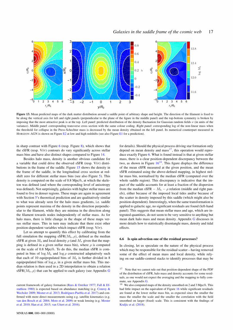
Galaxies in the saddle frame of the cosmic web 17
0 1 2 3 4 5 6-6
-4
-2
0
2
4
6
r/R0
r ///R0
-3 -2 -1 0 1 2 3-3
-2
-1
0
1
2
3
y/R0
x/R0
-0.4
-0.2
0
0.2
0.4
0.6
0.8
ν
0 1 2 3 4 5 6-6
-4
-2
0
2
4
6
r/R0
r ///R0
11.6
12.0
12.4
12.8
logM
h
Figure 13. Mean predicted maps of the dark matter distribution around a saddle point of arbitrary shape and height. The direction of the filament is fixed tobe along the vertical axis for left and right panels (perpendicular to the plane of the figure in the middle panel) and the top-bottom symmetry is broken byimposing that the most attractive peak is at the top. Left panel: predicted distribution of the density fluctuation for Gaussian random fields ν (in units of thevariance). Middle panel: corresponding transverse cross section with the same colour coding. Right panel: corresponding log of the non-linear mass whenthe threshold for collapse in the Press-Schechter mass is decreased by the mean density obtained on the left panel. Its numerical counterpart measured inHORIZON-AGN is shown on Figure E2 at low and high redshifts (see also Figure E1 for a prediction).
in sharp contrast with Figure 6 (resp. Figure 8), which shows thatthe sSFR (resp. V/σ) contours do vary significantly across stellarmass bins and have also distinct shapes compared to Figure 14.
Besides halo mass, density is another obvious candidate fora variable that could drive the observed sSFR (resp. V/σ) distri-butions in the frame of the saddle. Figure 15 shows the density inthe frame of the saddle, in the longitudinal cross section at red-shift zero for different stellar mass bins (see also Figure 5). Thisdensity is computed on the scale of 0.8 Mpc/h, at which the skele-ton was defined (and where the corresponding level of anisotropywas defined). Not surprisingly, galaxies with higher stellar mass arefound to live in denser regions. These maps are again in agreementwith Section 5’s theoretical prediction and are qualitatively similarto what was already seen for the halo mass gradients, i.e. saddlepoints represent maxima of the density in the direction perpendic-ular to the filament, while they are minima in the direction alongthe filament towards nodes independently of stellar mass. As forhalo mass, there is little change in the shape of these maps ver-sus stellar mass. This in turn may indicate that there exist otherposition-dependent variables which impact sSFR (resp. V/σ).
Let us attempt to quantify this effect by calibrating from thefull simulation the mapping ˆsSFR(Mh, ρ), defined as the mediansSFR at given Mh and local density ρ (and M? given that the map-ping is defined in a given stellar mass bin), where ρ is computedon the scale of 0.8 Mpc/h. To do this, the median sSFR is com-puted in bins of logMh and log ρ constructed adaptatively suchthat each of 10 equipopulated bins of Mh is further divided in 8equipopulated bins of log ρ, in a given stellar mass bin. This me-dian relation is then used in a 2D interpolation to obtain a relation
ˆsSFR(Mh, ρ) that can be applied to each galaxy (see Appendix G
current framework of galaxy formation (Rees & Ostriker 1977; Fall & Ef-stathiou 1980) is expected based on abundance matching (e.g. Conroy &Wechsler 2009; Moster et al. 2013; Rodrıguez-Puebla et al. 2017) and con-firmed with more direct measurements using e.g. satellite kinematics (e.g.van den Bosch et al. 2004; More et al. 2009) or weak lensing (e.g. Mosteret al. 2010; Han et al. 2015; van Uitert et al. 2016).
for details). Should the physical process driving star formation onlydepend on mean density and mass17, this operation would repro-duce exactly Figure 6. What is found instead is that at given stellarmass, there is a clear position-dependent discrepancy between thetwo, as shown in Figure 1618. This figure displays the differenceof the mean sSFR measured at the given position, and the meansSFR estimated using the above-defined mapping, in highest stel-lar mass bin, normalised by the median sSFR (computed over thewhole saddle region). This discrepancy is indicative that the im-pact of the saddle accounts for at least a fraction of the dispersionfrom the median sSFR −Mh − ρ relation (middle and right pan-els), either because of the imposed local tides and/or because ofthe scatter in density imposed by this saddle (which might also beposition-dependent). Interestingly, when the same transformation isapplied to galactic age, no significant residuals are found (left-handpanel). This suggests that mean stellar mass and age, which are in-tegrated quantities, do not seem to be very sensitive to anything butmean dark halo mass and mean density. Appendix G discusses inmore details how to statistically disentangle mass, density and tidaleffects.
6.6 Is spin advection one of the residual processes?
In closing, let us speculate on the nature of the physical processwhich may be responsible for the residual scatter – having removedsome of the effect of mean mass and local density, while rely-ing on our saddle-centred stacks to identify processes that may be
17 Note that we cannot rule out that position-dependent shape of the PDFof the distribution of sSFR, halo mass and density accounts for some resid-uals, as one would not expect the averaging and the mapping to fully com-mute, see Appendix G.18 We also computed maps of the density smoothed on 2 and 3 Mpc/h. Thishad little impact on the equivalent of Figure 16 while significant residualsare found at the lower stellar mass bin, as expected since the smaller themass the smaller the scale and the smaller the correlation with the fieldsmoothed on larger (fixed) scale. This is consistent with the findings ofKraljic et al. (2018).
MNRAS 000, 000–000 (0000)
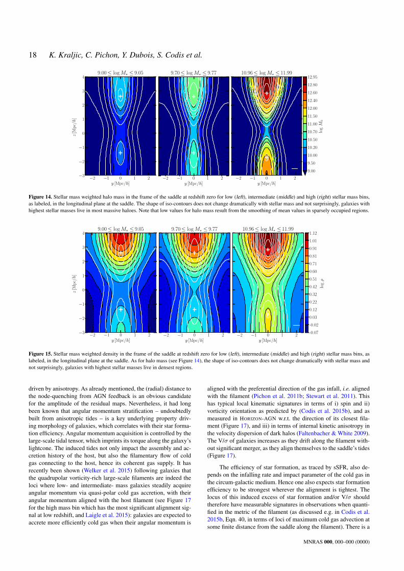
18 K. Kraljic, C. Pichon, Y. Dubois, S. Codis et al.
−2 −1 0 1 2y [Mpc/h]
−3
−2
−1
0
1
2
3
4z[M
pc/h]
9.00≤ logM⋆ ≤ 9.05
−2 −1 0 1 2y [Mpc/h]
9.70≤ logM⋆ ≤ 9.77
−2 −1 0 1 2y [Mpc/h]
10.96≤ logM⋆ ≤ 11.99
9.00
9.50
10.00
10.20
10.50
10.70
11.00
11.50
12.00
12.40
12.60
12.80
12.95
logM
h
Figure 14. Stellar mass weighted halo mass in the frame of the saddle at redshift zero for low (left), intermediate (middle) and high (right) stellar mass bins,as labeled, in the longitudinal plane at the saddle. The shape of iso-contours does not change dramatically with stellar mass and not surprisingly, galaxies withhighest stellar masses live in most massive haloes. Note that low values for halo mass result from the smoothing of mean values in sparsely occupied regions.
−2 −1 0 1 2y [Mpc/h]
−3
−2
−1
0
1
2
3
4
z[M
pc/h]
9.00≤ logM⋆ ≤ 9.05
−2 −1 0 1 2y [Mpc/h]
9.70≤ logM⋆ ≤ 9.77
−2 −1 0 1 2y [Mpc/h]
10.96≤ logM⋆ ≤ 11.99
-0.07
-0.02
0.03
0.12
0.22
0.32
0.42
0.51
0.60
0.71
0.81
0.91
1.01
1.12
logρ
Figure 15. Stellar mass weighted density in the frame of the saddle at redshift zero for low (left), intermediate (middle) and high (right) stellar mass bins, aslabeled, in the longitudinal plane at the saddle. As for halo mass (see Figure 14), the shape of iso-contours does not change dramatically with stellar mass andnot surprisingly, galaxies with highest stellar masses live in densest regions.
driven by anisotropy. As already mentioned, the (radial) distance tothe node-quenching from AGN feedback is an obvious candidatefor the amplitude of the residual maps. Nevertheless, it had longbeen known that angular momentum stratification – undoubtedlybuilt from anisotropic tides – is a key underlying property driv-ing morphology of galaxies, which correlates with their star forma-tion efficiency. Angular momentum acquisition is controlled by thelarge-scale tidal tensor, which imprints its torque along the galaxy’slightcone. The induced tides not only impact the assembly and ac-cretion history of the host, but also the filamentary flow of coldgas connecting to the host, hence its coherent gas supply. It hasrecently been shown (Welker et al. 2015) following galaxies thatthe quadrupolar vorticity-rich large-scale filaments are indeed theloci where low- and intermediate- mass galaxies steadily acquireangular momentum via quasi-polar cold gas accretion, with theirangular momentum aligned with the host filament (see Figure 17for the high mass bin which has the most significant alignment sig-nal at low redshift, and Laigle et al. 2015): galaxies are expected toaccrete more efficiently cold gas when their angular momentum is
aligned with the preferential direction of the gas infall, i.e. alignedwith the filament (Pichon et al. 2011b; Stewart et al. 2011). Thishas typical local kinematic signatures in terms of i) spin and ii)vorticity orientation as predicted by (Codis et al. 2015b), and asmeasured in HORIZON-AGN w.r.t. the direction of its closest fila-ment (Figure 17), and iii) in terms of internal kinetic anisotropy inthe velocity dispersion of dark halos (Faltenbacher & White 2009).The V/σ of galaxies increases as they drift along the filament with-out significant merger, as they align themselves to the saddle’s tides(Figure 17).
The efficiency of star formation, as traced by sSFR, also de-pends on the infalling rate and impact parameter of the cold gas inthe circum-galactic medium. Hence one also expects star formationefficiency to be strongest wherever the alignment is tightest. Thelocus of this induced excess of star formation and/or V/σ shouldtherefore have measurable signatures in observations when quanti-fied in the metric of the filament (as discussed e.g. in Codis et al.2015b, Eqn. 40, in terms of loci of maximum cold gas advection atsome finite distance from the saddle along the filament). There is a
MNRAS 000, 000–000 (0000)

Galaxies in the saddle frame of the cosmic web 19
−2 −1 0 1 2y [Mpc/h]
−3
−2
−1
0
1
2
3
4
z[M
pc/h]
11.0 11.5 12.0 12.5 13.0 13.5log Mh
0
1
2
logρ
10.96≤ logM⋆ ≤ 11.99
5.5
7.5
9.5
age[Gyr]
-0.030
-0.025
-0.020
-0.017
-0.014
-0.011
-0.007
0.000
∆age
−2 −1 0 1 2y [Mpc/h]
−3
−2
−1
0
1
2
3
4
z[M
pc/h]
11.0 11.5 12.0 12.5 13.0 13.5log Mh
0
1
2
logρ
10.96≤ logM⋆ ≤ 11.99
0.1
0.8
5.0
sSFR/10−
11[yr−
1]
0.20
0.30
0.40
0.45
0.50
0.55
0.65
0.75
0.79
0.83
∆sSFR
−2 −1 0 1 2y [Mpc/h]
−3
−2
−1
0
1
2
3
4
z[M
pc/h]
11.0 11.5 12.0 12.5 13.0 13.5log Mh
0
1
2
logρ
10.96≤ logM⋆ ≤ 11.99
0.02
0.10
0.50
V/σ
0.04
0.06
0.08
0.10
0.12
0.14
0.16
0.18
0.19
∆V/σ
Figure 16. Age, sSFR and V/σ residuals, from left to right, having removed the mean stellar mass, halo mass and density effects, respectively by binning andconsidering the median mapping (see text for details), in terms of fraction of the median values in the frame of the saddle at redshift zero for high stellar massbin, in the longitudinal plane at the saddle. The red dashed contours and the red crosses correspond to the galaxy number counts and the peaks in galacticdensity on axis, respectively and the red horizontal lines represent the smoothing length used in the analysis. The sub-panels on the top show the distributionsof the three parameters, age, sSFR and V/σ (in colours), as a function of halo mass,Mh and local density ρ (computed on the scale of 0.8 Mpc/h, at which theskeleton and the corresponding level of anisotropy were defined), respectively, with number counts overplotted in black. Interestingly, the residuals for sSFRand V/σ display an excess at finite distance between the saddle and the nodes, which points towards the expected loci of maximum spin up and limited AGNquenching. Conversely, the age residuals are very small (. 3%) relative to the values of residuals obtained for sSFR and V/σ, consistently with the observationthat the age, halo mass and local density gradients show many similarities (compare bottom panel of Figures 8, Figure 14 and Figure 15, respectively).
hint of such excess in the residuals shown in Figure 16 in terms ofboth sSFR and V/σ (which should co-evolve). While quenching isalso playing a significant position-dependent role for the high masspopulation, its impact on the lower mass galaxies will be less sig-nificant. Figure 18 shows indeed that for the lower mass bins, theresidual maps peak significantly on axis, which supports the ideathat the efficiency of angular momentum advection is a relevantprocess. This is worth emphasising, given the above-given theoreti-cal prejudices based on following galaxies in the flow (Welker et al.2015), and on the orientation of galaxies traced by their spin’s ori-entation distribution in the vicinity of the filament axis, predicted toexhibit a point-reflection symmetric structure (Codis et al. 2015b)as measured in Figure 17. While this discussion is more specula-tive, recall in any case that most properties of the galactic popu-lation measured within the frame of saddles presented in the pre-vious section – including redshift evolution and filament thicken-ing/thinning – can be understood when accounting for their cosmicadvection with the bulk flow along and transverse to the filament.The present study clearly highlighted that an improved model forgalaxy properties should also explicitly integrate the diversity ofthe topology of the large environment on multiple scales (follow-ing, e.g. Hanami 2001) and quantify the impact of its anisotropyon galactic mass assembly history, and more generally on the kine-matic history of galaxies. The details of how the kinematics impactstar formation remains to be understood. The vorticity-rich kine-matics of the large scale flow is neither strictly coherent nor fullyturbulent. Does the offset of merger and accretion rate imposedby the large scale turbulent flow explain the residual environmentdependence in observed physical properties (Aragon-Calvo et al.
2016), or is the helicity of gas inflow within filaments prevalent infeeding galactic discs coherently (Pichon et al. 2011a)?
7 CONCLUSIONS
This paper investigated the properties of virtual galaxies in theneighbourhood of filament-type saddle points of the cosmic web.These properties were measured within the frame set by the princi-pal axes of the saddle in the HORIZON-AGN simulation. The impactof AGN feedback was assessed by comparing to results obtainedin the HORIZON-NOAGN simulation. The principal findings are thefollowing:
• The iso-contours of the galactic number density, mass, sSFR, V/σand age in the saddle’s frame display a clear alignment with thefilament axis and stronger gradients perpendicular to the filaments,quantifying the impact of the cosmic web in shaping galaxies.• High mass galaxies are more clustered around filaments and
within filaments around nodes compared to their low mass counter-parts. As expected, the filament’s width of the whole galaxy pop-ulation grows with cosmic time (as it becomes dominated by lessrare galaxies). Conversely, at fixed mass, it decreases with cosmictime at the saddle.• In addition to reducing the overall sSFR of galaxies, AGN feed-
back also impacts the shape of the sSFR iso-contours, in particularfor high mass galaxies and in the vicinity of the nodes of the cosmicweb. AGN feedback quenches centrals more efficiently than satel-lites. Satellite strangulation seems to occur within the filaments andnodes of the cosmic web.• While the dominant effect of the cosmic web on galaxy formation
MNRAS 000, 000–000 (0000)

20 K. Kraljic, C. Pichon, Y. Dubois, S. Codis et al.
−1.5 −1.0 −0.5 0.0 0.5 1.0 1.5y [Mpc/h]
−1.5
−1.0
−0.5
0.0
0.5
1.0
1.5
x[M
pc/h]
10.96≤ logM⋆ ≤ 11.99
-0.381-0.331-0.282-0.232-0.183-0.133-0.084-0.0340.0150.0650.1140.1640.2130.2630.312
cosθ
−1.5 −1.0 −0.5 0.0 0.5 1.0 1.5y [Mpc/h]
−1.5
−1.0
−0.5
0.0
0.5
1.0
1.5
x[M
pc/h]
10.96≤ logM⋆ ≤ 11.99
-0.579-0.504-0.428-0.353-0.277-0.202-0.126-0.0510.0250.1000.1760.2510.3270.4020.478
cosβ
Figure 17. Stellar mass-weighted cosine of angle between the spin of thegalaxy and the direction of the filament (top panel) and between the vor-ticity of the gas at the position of the galaxy and the direction of the fil-ament (bottom panel) for highest stellar mass bin at redshift zero. Trans-verse cross-sections comprise galaxies with z-coordinate between 1 and 2.5Mpc/h for the spin and between 0.5 and 1.8 Mpc/h for the vorticity, wherethe signal is most significant. The vorticity is computed on the gas distri-bution at the resolution and smoothing length used to define the skeleton,and interpolated at the position of galaxies. The map is normalised so thatthe integrated amplitude in each quadrant is preserved while smoothing.The white contours and the white crosses correspond to the galaxy numbercounts and the peaks in galactic density, respectively. Note the quadrupolar(point-reflection symmetric) structure of the spin’s orientation distributionin the vicinity of the filament axis, in qualitative agreement with the predic-tion of Codis et al. (2015b) for dark matter. The distribution of the vorticityof the gas is also in qualitative agreement with this prediction and with themeasurement of Laigle et al. (2015) (their Appendix A), which focused oncooling runs (without star formation). The tilt in the plane of symmetry ofthe vorticity map is likely to be driven by shot noise.
seems to be captured by the distance to cosmic nodes, the full threedimensional geometry of the web, in particular its saddle points,provides a natural oriented frame for stacking galaxies, showingsignificant effects of the environment beyond solely the distanceto nodes. Hence, galaxies do retain a memory of the large-scalecosmic flows from which they emerged.• The redshift evolution of the galactic counts and the age distribu-
tion of galaxies are consistent with a drift of the population towards
−2 −1 0 1 2y [Mpc/h]
−3
−2
−1
0
1
2
3
4
z[M
pc/h]
10.0 10.5 11.0log Mh
0
1
2
logρ
9.00≤ logM⋆ ≤ 9.05
AGN
−2 −1 0 1 2y [Mpc/h]
10.0 10.5 11.0log Mh
9.00≤ logM⋆ ≤ 9.05
0.005
0.020
0.080
0.300
V/σ
-0.01
0.00
0.02
0.04
0.06
0.07
0.09
0.10
0.12
0.14
∆V/σ
noAGN
Figure 18. V/σ residuals in HORIZON-AGN (left panel) andHORIZON-NOAGN (right panel), having removed the mean stellarmass, halo mass and density effects, respectively by binning and consider-ing the median mapping (see text), in the lowest stellar mass bin at redshiftzero. The red dashed contours and the red crosses correspond to the galaxynumber counts and the peaks in galactic density on axis, respectively andthe red horizontal lines represent the smoothing length used in the analysis.The two maps are qualitatively similar, as expected for this mass binwhere AGN feedback should not have a strong impact, and nonetheless theamplitude of the map is ∼ 14%, concentrated along the filament’s axis.
the filaments and along them (see Appendix F). The cosmic evolu-tion of the sSFR reflects both this drift and the triggering of quench-ing as centrals become massive enough to trigger AGN feedbacknear the peaks of the cosmic web. The geometry of the stacks andtheir cosmic evolution compare favourably to expectations for con-strained Gaussian random fields in the weakly non-linear regime.• The maps of V/σ and sSFR (and their residuals) are consistent
with the role played by feedback and angular momentum in shapinggalaxies, beyond that played by mass and density, and its connec-tion with the geometry of the cosmic web, as described by Codiset al. (2015b) and Laigle et al. (2015) (in a Lagrangian and an Eule-rian framework, respectively). The point-reflection symmetric dis-tribution of the orientation of the spin of galaxies and vorticity ofthe gas presented in this paper is also in agreement with this picture.• At high mass and low redshift, AGN feedback coupled with
advection of galaxies along filaments induces some level ofanisotropy in the distribution of galaxy properties (sSFR, V/σ, age)which is partially degenerate with the effect of how angular mo-mentum of galaxies is acquired from the large-scale vorticity of theanisotropic environment.• While sSFR responds to the saddle frame over and above what is
expected from halo mass and local density, other indicators such asstellar age do not.
Overall, all distributions are consistent with the geometry of theflow in the vicinity of saddles, including quenching by AGN feed-back, strangulation of satellites near the nodes, and possibly timedelays induced by asymmetric tides on local and intermediatescales. They complement the findings of Kraljic et al. (2018), whichalso showed that galaxy properties occupy more than a two dimen-sional manifold (in physical parameter space such as age, sSFR,
MNRAS 000, 000–000 (0000)
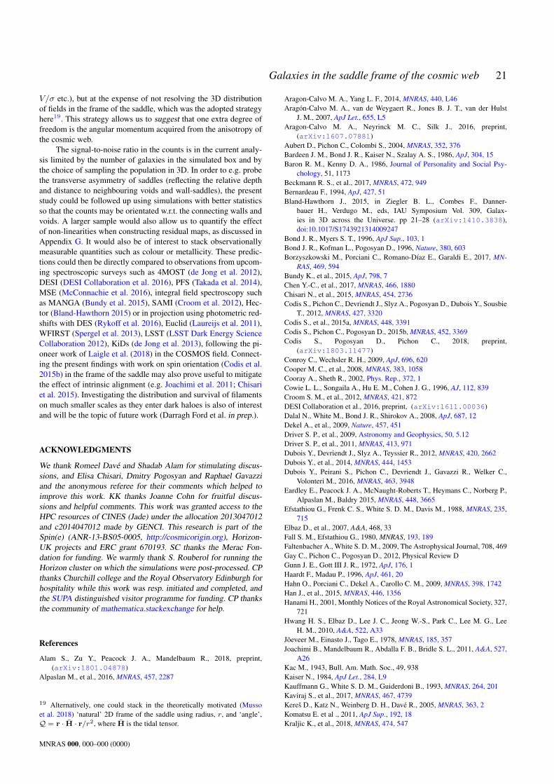
Galaxies in the saddle frame of the cosmic web 21
V/σ etc.), but at the expense of not resolving the 3D distributionof fields in the frame of the saddle, which was the adopted strategyhere19. This strategy allows us to suggest that one extra degree offreedom is the angular momentum acquired from the anisotropy ofthe cosmic web.
The signal-to-noise ratio in the counts is in the current analy-sis limited by the number of galaxies in the simulated box and bythe choice of sampling the population in 3D. In order to e.g. probethe transverse asymmetry of saddles (reflecting the relative depthand distance to neighbouring voids and wall-saddles), the presentstudy could be followed up using simulations with better statisticsso that the counts may be orientated w.r.t. the connecting walls andvoids. A larger sample would also allow us to quantify the effectof non-linearities when constructing residual maps, as discussed inAppendix G. It would also be of interest to stack observationallymeasurable quantities such as colour or metallicity. These predic-tions could then be directly compared to observations from upcom-ing spectroscopic surveys such as 4MOST (de Jong et al. 2012),DESI (DESI Collaboration et al. 2016), PFS (Takada et al. 2014),MSE (McConnachie et al. 2016), integral field spectroscopy suchas MANGA (Bundy et al. 2015), SAMI (Croom et al. 2012), Hec-tor (Bland-Hawthorn 2015) or in projection using photometric red-shifts with DES (Rykoff et al. 2016), Euclid (Laureijs et al. 2011),WFIRST (Spergel et al. 2013), LSST (LSST Dark Energy ScienceCollaboration 2012), KiDs (de Jong et al. 2013), following the pi-oneer work of Laigle et al. (2018) in the COSMOS field. Connect-ing the present findings with work on spin orientation (Codis et al.2015b) in the frame of the saddle may also prove useful to mitigatethe effect of intrinsic alignment (e.g. Joachimi et al. 2011; Chisariet al. 2015). Investigating the distribution and survival of filamentson much smaller scales as they enter dark haloes is also of interestand will be the topic of future work (Darragh Ford et al. in prep.).
ACKNOWLEDGMENTS
We thank Romeel Dave and Shadab Alam for stimulating discus-sions, and Elisa Chisari, Dmitry Pogosyan and Raphael Gavazziand the anonymous referee for their comments which helped toimprove this work. KK thanks Joanne Cohn for fruitful discus-sions and helpful comments. This work was granted access to theHPC resources of CINES (Jade) under the allocation 2013047012and c2014047012 made by GENCI. This research is part of theSpin(e) (ANR-13-BS05-0005, http://cosmicorigin.org), Horizon-UK projects and ERC grant 670193. SC thanks the Merac Fon-dation for funding. We warmly thank S. Rouberol for running theHorizon cluster on which the simulations were post-processed. CPthanks Churchill college and the Royal Observatory Edinburgh forhospitality while this work was resp. initiated and completed, andthe SUPA distinguished visitor programme for funding. CP thanksthe community of mathematica.stackexchange for help.
References
Alam S., Zu Y., Peacock J. A., Mandelbaum R., 2018, preprint,(arXiv:1801.04878)
Alpaslan M., et al., 2016, MNRAS, 457, 2287
19 Alternatively, one could stack in the theoretically motivated (Mussoet al. 2018) ‘natural’ 2D frame of the saddle using radius, r, and ‘angle’,Q = r · H · r/r2, where H is the tidal tensor.
Aragon-Calvo M. A., Yang L. F., 2014, MNRAS, 440, L46Aragon-Calvo M. A., van de Weygaert R., Jones B. J. T., van der Hulst
J. M., 2007, ApJ Let., 655, L5Aragon-Calvo M. A., Neyrinck M. C., Silk J., 2016, preprint,
(arXiv:1607.07881)Aubert D., Pichon C., Colombi S., 2004, MNRAS, 352, 376Bardeen J. M., Bond J. R., Kaiser N., Szalay A. S., 1986, ApJ, 304, 15Baron R. M., Kenny D. A., 1986, Journal of Personality and Social Psy-
chology, 51, 1173Beckmann R. S., et al., 2017, MNRAS, 472, 949Bernardeau F., 1994, ApJ, 427, 51Bland-Hawthorn J., 2015, in Ziegler B. L., Combes F., Danner-
bauer H., Verdugo M., eds, IAU Symposium Vol. 309, Galax-ies in 3D across the Universe. pp 21–28 (arXiv:1410.3838),doi:10.1017/S1743921314009247
Bond J. R., Myers S. T., 1996, ApJ Sup., 103, 1Bond J. R., Kofman L., Pogosyan D., 1996, Nature, 380, 603Borzyszkowski M., Porciani C., Romano-Dıaz E., Garaldi E., 2017, MN-
RAS, 469, 594Bundy K., et al., 2015, ApJ, 798, 7Chen Y.-C., et al., 2017, MNRAS, 466, 1880Chisari N., et al., 2015, MNRAS, 454, 2736Codis S., Pichon C., Devriendt J., Slyz A., Pogosyan D., Dubois Y., Sousbie
T., 2012, MNRAS, 427, 3320Codis S., et al., 2015a, MNRAS, 448, 3391Codis S., Pichon C., Pogosyan D., 2015b, MNRAS, 452, 3369Codis S., Pogosyan D., Pichon C., 2018, preprint,
(arXiv:1803.11477)Conroy C., Wechsler R. H., 2009, ApJ, 696, 620Cooper M. C., et al., 2008, MNRAS, 383, 1058Cooray A., Sheth R., 2002, Phys. Rep., 372, 1Cowie L. L., Songaila A., Hu E. M., Cohen J. G., 1996, AJ, 112, 839Croom S. M., et al., 2012, MNRAS, 421, 872DESI Collaboration et al., 2016, preprint, (arXiv:1611.00036)Dalal N., White M., Bond J. R., Shirokov A., 2008, ApJ, 687, 12Dekel A., et al., 2009, Nature, 457, 451Driver S. P., et al., 2009, Astronomy and Geophysics, 50, 5.12Driver S. P., et al., 2011, MNRAS, 413, 971Dubois Y., Devriendt J., Slyz A., Teyssier R., 2012, MNRAS, 420, 2662Dubois Y., et al., 2014, MNRAS, 444, 1453Dubois Y., Peirani S., Pichon C., Devriendt J., Gavazzi R., Welker C.,
Volonteri M., 2016, MNRAS, 463, 3948Eardley E., Peacock J. A., McNaught-Roberts T., Heymans C., Norberg P.,
Alpaslan M., Baldry 2015, MNRAS, 448, 3665Efstathiou G., Frenk C. S., White S. D. M., Davis M., 1988, MNRAS, 235,
715Elbaz D., et al., 2007, A&A, 468, 33Fall S. M., Efstathiou G., 1980, MNRAS, 193, 189Faltenbacher A., White S. D. M., 2009, The Astrophysical Journal, 708, 469Gay C., Pichon C., Pogosyan D., 2012, Physical Review DGunn J. E., Gott III J. R., 1972, ApJ, 176, 1Haardt F., Madau P., 1996, ApJ, 461, 20Hahn O., Porciani C., Dekel A., Carollo C. M., 2009, MNRAS, 398, 1742Han J., et al., 2015, MNRAS, 446, 1356Hanami H., 2001, Monthly Notices of the Royal Astronomical Society, 327,
721Hwang H. S., Elbaz D., Lee J. C., Jeong W.-S., Park C., Lee M. G., Lee
H. M., 2010, A&A, 522, A33Joeveer M., Einasto J., Tago E., 1978, MNRAS, 185, 357Joachimi B., Mandelbaum R., Abdalla F. B., Bridle S. L., 2011, A&A, 527,
A26Kac M., 1943, Bull. Am. Math. Soc., 49, 938Kaiser N., 1984, ApJ Let., 284, L9Kauffmann G., White S. D. M., Guiderdoni B., 1993, MNRAS, 264, 201Kaviraj S., et al., 2017, MNRAS, 467, 4739Keres D., Katz N., Weinberg D. H., Dave R., 2005, MNRAS, 363, 2Komatsu E. et al ., 2011, ApJ Sup., 192, 18Kraljic K., et al., 2018, MNRAS, 474, 547
MNRAS 000, 000–000 (0000)
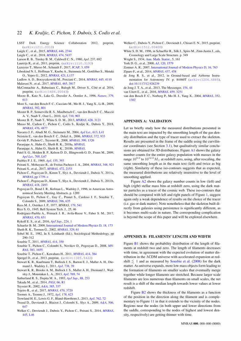
22 K. Kraljic, C. Pichon, Y. Dubois, S. Codis et al.
LSST Dark Energy Science Collaboration 2012, preprint,(arXiv:1211.0310)
Laigle C., et al., 2015, MNRAS, 446, 2744Laigle C., et al., 2018, MNRAS, 474, 5437Larson R. B., Tinsley B. M., Caldwell C. N., 1980, ApJ, 237, 692Laureijs R., et al., 2011, preprint, (arXiv:1110.3193)Lazeyras T., Musso M., Schmidt F., 2017, JCAP, 3, 059Libeskind N. I., Hoffman Y., Knebe A., Steinmetz M., Gottlober S., Metuki
O., Yepes G., 2012, MNRAS, 421, L137Ludlow A. D., Borzyszkowski M., Porciani C., 2014, MNRAS, 445, 4110Malavasi N., et al., 2017, MNRAS, 465, 3817McConnachie A., Babusiaux C., Balogh M., Driver S., Cote et al. 2016,
preprint, (arXiv:1606.00043)Moore B., Katz N., Lake G., Dressler A., Oemler A., 1996, Nature, 379,
613More S., van den Bosch F. C., Cacciato M., Mo H. J., Yang X., Li R., 2009,
MNRAS, 392, 801Moster B. P., Somerville R. S., Maulbetsch C., van den Bosch F. C., Maccio
A. V., Naab T., Oser L., 2010, ApJ, 710, 903Moster B. P., Naab T., White S. D. M., 2013, MNRAS, 428, 3121Musso M., Cadiou C., Pichon C., Codis S., Kraljic K., Dubois Y., 2018,
MNRAS, 476, 4877Navarro J. F., Abadi M. G., Steinmetz M., 2004, ApJ Let., 613, L41Neistein E., van den Bosch F. C., Dekel A., 2006, MNRAS, 372, 933Ocvirk P., Pichon C., Teyssier R., 2008, MNRAS, 390, 1326Paranjape A., Hahn O., Sheth R. K., 2018a, MNRAS,Paranjape A., Hahn O., Sheth R. K., 2018b, MNRAS,Patel S. G., Holden B. P., Kelson D. D., Illingworth G. D., Franx M., 2009,
ApJ Let., 705, L67Peebles P. J. E., 1969, ApJ, 155, 393Peirani S., Mohayaee R., de Freitas Pacheco J. A., 2004, MNRAS, 348, 921Peirani S., et al., 2017, MNRAS, 472, 2153Pichon C., Pogosyan D., Kimm T., Slyz A., Devriendt J., Dubois Y., 2011a,
MNRAS, pp 1739–+Pichon C., Pogosyan D., Kimm T., Slyz A., Devriendt J., Dubois Y., 2011b,
MNRAS, 418, 2493Pogosyan D., Bond J. R., Kofman L., Wadsley J., 1996, in American Astro-
nomical Society Meeting Abstracts. p. 1289Pogosyan D., Pichon C., Gay C., Prunet S., Cardoso J. F., Sousbie T.,
Colombi S., 2009, MNRAS, 396, 635Rees M. J., Ostriker J. P., 1977, MNRAS, 179, 541Rice S. O., 1945, Bell System Tech. J., 25, 46Rodrıguez-Puebla A., Primack J. R., Avila-Reese V., Faber S. M., 2017,
MNRAS, 470, 651Rykoff E. S., et al., 2016, ApJ Sup., 224, 1Schaefer B. M., 2009, International Journal of Modern Physics D, 18, 173Sheth R. K., Tormen G., 2002, MNRAS, 329, 61Sobel M. E., 1982, In S. Leinhardt (Ed.), Sociological Methodology, pp
290–312Sousbie T., 2011, MNRAS, 414, 350Sousbie T., Pichon C., Colombi S., Novikov D., Pogosyan D., 2008, MN-
RAS, 383, 1655Sousbie T., Pichon C., Kawahara H., 2011, MNRAS, 414, 384Spergel D., et al., 2013, preprint, (arXiv:1305.5422)Stewart K. R., Kaufmann T., Bullock J. S., Barton E. J., Maller A. H., Die-
mand J., Wadsley J., 2011, ApJ, 738, 39Stewart K. R., Brooks A. M., Bullock J. S., Maller A. H., Diemand J., Wad-
sley J., Moustakas L. A., 2013, ApJ, 769, 74Sutherland R. S., Dopita M. A., 1993, ApJ Sup., 88, 253Takada M., et al., 2014, PASJ, 66, R1Teyssier R., 2002, A&A, 385, 337Tojeiro R., et al., 2017, MNRAS, 470, 3720Toomre A., Toomre J., 1972, ApJ, 178, 623Trowland H. E., Lewis G. F., Bland-Hawthorn J., 2013, ApJ, 762, 72Tweed D., Devriendt J., Blaizot J., Colombi S., Slyz A., 2009, A&A, 506,
647Welker C., Devriendt J., Dubois Y., Pichon C., Peirani S., 2014, MNRAS,
445, L46
Welker C., Dubois Y., Pichon C., Devriendt J., Chisari E. N., 2015, preprint,(arXiv:1512.00400)
White S. D. M., 1996, in Schaeffer R., Silk J., Spiro M., Zinn-Justin J., eds,Cosmology and Large Scale Structure. p. 349
Wright S., 1934, Ann. Math. Statist., 5, 161York D. G., et al., 2000, AJ, 120, 1579Zentner A. R., 2007, International Journal of Modern Physics D, 16, 763Ziparo F., et al., 2014, MNRAS, 437, 458de Jong R. S., et al., 2012, in Ground-based and Airborne Instru-
mentation for Astronomy IV. p. 84460T (arXiv:1206.6885),doi:10.1117/12.926239
de Jong J. T. A., et al., 2013, The Messenger, 154, 44van Uitert E., et al., 2016, MNRAS, 459, 3251van den Bosch F. C., Norberg P., Mo H. J., Yang X., 2004, MNRAS, 352,
1302
APPENDIX A: VALIDATION
Let us briefly study how the measured distributions presented inthe main text are impacted by the smoothing length of the gas den-sity distribution and the type of tracer used to extract the skeleton.Results are presented in the frame of the saddle using the curvilin-ear coordinates (see Section 3.1), but qualitatively similar conclu-sions are obtained for 3D distributions. Figure A1 shows the galaxynumber counts for the entire galaxy population with masses in therange 109.0 to 1012.0M at redshift zero, using, after rescaling, thesame smoothing length as in the main text (left) and twice as big(right). Similarity of these iso-contours suggests that as expected,the measured distributions are relatively insensitive to the level ofsmoothing applied.
Figure A2 shows the galaxy number counts in low (left) andhigh (right) stellar mass bins at redshift zero, using the dark mat-ter particles as a tracer of the cosmic web. These iso-contours thatshould be compared with left and right panels of Figure 1, suggestagain only a weak dependence of results on the choice of the tracer(i.e. gas or dark matter). Note nonetheless that the skeleton built di-rectly from galaxies using persistence is significantly different, asit becomes multi-scale in nature. The corresponding complicationis beyond the scope of this paper and will be explored elsewhere.
APPENDIX B: FILAMENTS’ LENGTH AND WIDTH
Figure B1 shows the probability distribution of the length of fila-ments at redshift two and zero. The length of filaments decreaseswith time, in agreement with the expected evolution of matter dis-tribution in the ΛCDM universe with accelerated expansion at red-shift . 1 and as measured by Sousbie et al. (2008) for the darkmatter. As universe expands, more low mass objects form leading tothe formation of filaments on smaller scales that eventually mergetogether while longer filaments are stretched. Because larger scalefilaments are less numerous than filaments on small scales, the netresult is a shift of the median length towards lower values at lowerredshift.
Figure B2 shows the thickness of the filaments as a functionof the position in the direction along the filament and is comple-mentary to Figure 11 in that it extends to the vicinity of the nodes.Regions near the nodes (in both upper and lower directions fromthe saddle, corresponding to the nodes of highest and lowest den-sity, respectively) are getting thinner with time.
MNRAS 000, 000–000 (0000)
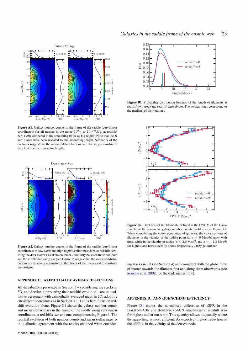
Galaxies in the saddle frame of the cosmic web 23
0.0 0.5 1.0 1.5R/Rs [Mpc/h]
−1.5
−1.0
−0.5
0.0
0.5
1.0
1.5
2.0
z/R
s[M
pc/h]
[9.00,11.99]
0.30.71.11.5
0.1 0.4PDF
0.0 0.5 1.0 1.5R/Rs [Mpc/h]
×2
[9.00,11.99]
0.1 0.4PDF
0.1
86.5
172.9
259.3
345.7
432.2
518.6
605.0
number
counts
Smoothing
Figure A1. Galaxy number counts in the frame of the saddle (curvilinearcoordinates) for all masses in the range 109.0 to 1012.0M at redshiftzero (left) compared to the smoothing twice as big (right). Note that the Rand z axes have been rescaled by the smoothing length. Similarity of thecontours suggest that the measured distributions are relatively insensitive tothe choice of the smoothing length.
0 1 2
R [Mpc/h]
−2
−1
0
1
2
3
z[M
pc/h]
[9.00,9.05]
0.2
1.0
1.8
0.1 0.3PDF
0 1 2
R [Mpc/h]
[10.93,11.99]
0.1 0.3PDF
0
2
4
6
8
10
12
14
number
counts
Dark matter
Figure A2. Galaxy number counts in the frame of the saddle (curvilinearcoordinates) in low (left) and high (right) stellar mass bins at redshift zero,using the dark matter as a skeleton tracer. Similarity between these contoursand those obtained using gas (see Figure 1) suggest that the measured distri-butions are relatively insensitive to the choice of the tracer used to constructthe skeleton.
APPENDIX C: AZIMUTHALLY AVERAGED SECTIONS
All distributions presented in Section 3 – considering the stacks in3D, and Section 4 presenting their redshift evolution – are in qual-itative agreement with azimuthally averaged maps in 2D, adoptingcurvilinear coordinates as in Section 3.1. Let us here focus on red-shift evolution alone. Figure C1 shows the galaxy number countsand mean stellar mass in the frame of the saddle using curvilinearcoordinates, at redshifts two and one, complementing Figure 1. Theredshift evolution of both number counts and mean stellar mass isin qualitative agreement with the results obtained when consider-
0 5 10 15 20 25length [Mpc/h]
0.00
0.02
0.04
0.06
0.08
0.10
0.12
0.14
0.16
0.18
PDF redshift=0
redshift=2
Figure B1. Probability distribution function of the length of filaments atredshift two (red) and redshift zero (blue). The vertical lines correspond tothe medians of distributions.
−2
−1
0
1
2
3
z[M
pc/h]
(a)
1.2 1.3 1.4 1.5 1.6 1.7
FWHM[Mpc/h]
−2
−1
0
1
2
3
z[M
pc/h]
redshift=0
redshift=2
(b)
Figure B2. Thickness of the filaments, defined as the FWHM of the Gaus-sian fit of the transverse galaxy number counts profiles as in Figure 11.When considering the entire population of galaxies, the cross sections offilaments in the vicinity of the saddle point (at z = 0 Mpc/h) grow withtime, while in the vicinity of nodes (z ∼ 2.5 Mpc/h and z ∼ −1.5 Mpc/hfor highest and lowest density nodes, respectively), they get thinner.
ing stacks in 3D (see Section 4) and consistent with the global flowof matter towards the filament first and along them afterwards (seeSousbie et al. 2008, for the dark matter flow).
APPENDIX D: AGN QUENCHING EFFICIENCY
Figure D1 shows the normalised difference of sSFR in theHORIZON-AGN and HORIZON-NOAGN simulations at redshift zerofor highest stellar mass bin. This quantity allows to quantify wherethe quenching is most efficient. As expected, highest reduction ofthe sSFR is in the vicinity of the densest node.
MNRAS 000, 000–000 (0000)

24 K. Kraljic, C. Pichon, Y. Dubois, S. Codis et al.
−2
−1
0
1
2
3
z[M
pc/h]
[9.00,9.03]
0.2
0.6
1.0
PDF [9.47,9.52] [10.46,11.72]
0
1
2
3
4
5
6
7
8
9
10
11
number
counts
[9.00,11.72]
0.250.350.450.55
9.10
9.40
9.50
9.60
9.70
9.80
9.90
9.95
10.00
10.05
10.10
10.15
10.20
10.25
10.30
10.35
10.40
logM
⋆
redshift=2.0
0 1 2
R [Mpc/h]
−2
−1
0
1
2
3
z[M
pc/h]
[9.00,9.04]
0.2
0.6
1.0
0.0 0.2PDF
0 1 2
R [Mpc/h]
[9.58,9.64]
0.0 0.2PDF
0 1 2
R [Mpc/h]
[10.68,11.92]
0.0 0.2PDF
0
1
2
3
4
5
6
7
8
9
10
11
number
counts
0 1 2R [Mpc/h]
[9.00,11.92]
0.250.350.450.55
0.0 0.1 0.2PDF
9.10
9.40
9.50
9.60
9.70
9.80
9.90
9.95
10.00
10.05
10.10
10.15
10.20
10.25
10.30
10.35
10.40
logM
⋆
redshift=1.0
Figure C1. Left and middle panels: Redshift evolution of the galaxy number counts in low (left column), intermediate (middle column) and high (rightcolumn) stellar mass bins, in the frame of the saddle (curvilinear coordinates) at redshift two (top row) and one (bottom row), respectively. The whitehorizontal lines represent the smoothing length used in the analysis. Rightmost panels: Redshift evolution of mean stellar mass iso-contours in the frame ofthe saddle (curvilinear coordinates) for the entire galaxy population at redshift two (top row) and one (bottom row), respectively. The white curves correspondto the contours of the galaxy number counts, while the white crosses represent the peaks in galactic number density on axis. Note how galaxies become moreclustered towards filaments and nodes as they grow in mass with decreasing redshift, consistently with the global flow of matter within the cosmic web and inagreement with results considering the 3D distributions.
APPENDIX E: THEORETICAL PREDICTIONS
Let us briefly predict from first principles the expected shape ofthe matter and halo distribution in the vicinity of a saddle and itscosmic evolution.
E1 Predictions for the mean constrained initial density field
The initial density field in which the cosmic web develops beingGaussian, the theory of constrained Gaussian random field providesa natural framework in which to compute the expectation of thematter distribution and typical halo mass within the frame set by thesaddle point, as we do not expect the dynamics to be strongly non-linear on such scales. An important ingredient here is therefore toimpose a filament-type saddle point constraint. Such a critical pointform when the gradient of the density field is zero and is defined byits geometry, namely i) its height ν defined as the density contrastdivided by its rms σ0 =
√〈δ2〉 and ii) its curvature by means of
the three eigenvalues of the Hessian matrix of the density contrastrescaled again by their rms σ2 =
√〈(∆δ)2〉. For a filament-type
saddle point, λ1 > 0 > λ2 > λ3.
The so-called peak theory (Kac 1943; Rice 1945) then al-lows us to predict all statistical properties of critical points oncethe (supposedly Gaussian here) probability density function (PDF)of the field ν = δ/σ0, its first νi = δ,i/σ1 and second derivativesνij = δ,ij/σ2 is known. The saddle constraint reads
Csad =1
R3?λ1λ2λ3ΘH(λ1)ΘH(−λ2)δD(νi) , (E1)
where the Dirac delta function ensures the gradient to be zero, theHeaviside Theta functions impose the sign of the eigenvalues, theJacobian λ1λ2λ3 = det νij accounts for the volume associatedwith a saddle point and R? = σ2/σ1.
To predict the mean density map around a saddle point, onehas to consider the joint statistics of (ν, νi, νij) together with thedensity field ν′ at a distance r from the saddle point. In addition,the symmetry along the axis of the filament (i = 1 here) will bebroken by imposing the first axis to be oriented in the opposite di-rection from that of the gradient of the gravitational potential (i.etowards the deepest potential well, the most attractive node). Onetherefore also has to consider Φ1 the derivative of the gravitationalpotential along the first direction rescaled by its corresponding vari-ance σ−1 =
√〈(∇Φ)2〉. Let us gather those 12 fields in a vec-
MNRAS 000, 000–000 (0000)

Galaxies in the saddle frame of the cosmic web 25
−2 −1 0 1 2y [Mpc/h]
−3
−2
−1
0
1
2
3
4
z[M
pc/h]
10.96≤ logM⋆ ≤ 11.99
-0.75
-0.73
-0.70
-0.65
-0.60
-0.55
-0.45
-0.35
-0.25
-0.15
-0.05
sSFR(A
GN)/sSFR(noA
GN)-1
Figure D1. sSFR ratio in the HORIZON-AGN, sSFR (AGN), andHORIZON-NOAGN, sSFR (noAGN), simulations at redshift zero for high-est stellar mass bin. Note that the highest impact of AGN feedback on sSFRof galaxies is, as expected, in the vicinity of the densest node. White con-tours represent galaxy number counts in the HORIZON-AGN simulation.
0 1 2 3
x [Mpc/h]
−3
−2
−1
0
1
2
3
z[M
pc/h]
0 1 2 3
x [Mpc/h]
−3
−2
−1
0
1
2
3
y[M
pc/h]
9
10
11
12
13
logM
h
Figure E1. Coloured contours: predicted cross section of the halo massdensity after a Zel’dovich boost for a fixed geometry of the saddle in theplane of the wall and filament (left panel) and perpendicular to the filament(right panel). Dashed contours: the cross section before the boost.
tor X = ν′, ν, ν1, ν2, ν3, ν11, ν22, ν33, ν12, ν13, ν23,Φ1 whosePDF can be written
P(X) =1√
det|2πC|exp
(−1
2XT ·C−1 ·X
), (E2)
where the covariance matrix C = 〈X · XT〉 depends on the sep-aration vector r and the linear power spectrum Pk(k) which caninclude a filter function on a given scale. In this work, a Λ-CDMpower spectrum is used (using the same values for the cosmologi-cal parameters as HORIZON-AGN) with a Gaussian filter defined in
0
0.1
0.2
0.3
0.3
0.4
0.4
0.5
0.5
0.6
0.6
0.7
0 1 2 3 4 5 6-6
-4
-2
0
2
4
6
r/R0
r ///R0
-0.2-0.1
0
0.1
0.2
0.3
0.4
0.5
0.6
0.6
0.7
0.7
0 1 2 3 4 5 6-6
-4
-2
0
2
4
6
r/R0
r ///R0
Figure E2. Left panel: dark matter longitudinal cross section measurementsin HORIZON-AGN at redshift 0. Right panel: same quantity at redshift 2.The corresponding prediction at high redshift is shown in Figure 13 and theagreement is fairly good.
Fourier space by
WG(k, L) =1
(2π)3/2exp
(−k2L2
2
), (E3)
with L = 0.8Mpc/h. One-point covariances do not depend onthe separation but may depend on the spectral parameter γ =σ2
1/(σ0σ2). The variance of the density field is one by definition,C11 = 1, while the diagonal block corresponding to the saddleposition, C0 = (Cij)i,j>1, reads
C0 =
1 0 0 0 −γ/3−γ/3−γ/3 0 0 0 00 1/3 0 0 0 0 0 0 0 0 −β/30 0 1/3 0 0 0 0 0 0 0 0
0 0 0 1/3 0 0 0 0 0 0 0−γ/3 0 0 0 1/5 1/15 1/15 0 0 0 0−γ/3 0 0 0 1/15 1/5 1/15 0 0 0 0
−γ/3 0 0 0 1/15 1/15 1/5 0 0 0 00 0 0 0 0 0 0 1/15 0 0 0
0 0 0 0 0 0 0 0 1/15 0 0
0 0 0 0 0 0 0 0 0 1/15 00 −β/3 0 0 0 0 0 0 0 0 1/3
,
with β = σ20/σ−1σ1. The cross correlations between ν′ and the
fields at the position of the saddle are to be computed carefullyas they depend on both the separation and the orientation of theseparation vector in the frame of the Hessian described by the co-ordinates with indices i = 1, 2, 3. They are explicit function of theshape of the power spectrum and are therefore computed numeri-cally (the angle dependence is analytical, hence only the integrationw.r.t k = |k| requires a numerical integration). They read for j be-tween 2 and 12
⟨ν′Xj
⟩=
∫d3kPk(k)
3∏i=1
(−ıki)αi(ık)−2p exp (ık · r)
∫d3kPk(k)
∫d3kPk(k)
3∏i=1
k2αii
, (E4)
where p = 1 only for j = 12 (because of Poisson equation) andzero elsewhere and αi counts the number of derivatives w.r.t indexi. Note that the mean density map around a saddle point of fixedheight and curvatures with no symmetry breaking (i.e not imposing
MNRAS 000, 000–000 (0000)

26 K. Kraljic, C. Pichon, Y. Dubois, S. Codis et al.
Φ1 < 0) is analytical and given by (Codis et al. 2015b)
⟨ν′|S
⟩=
(λ1+λ2+λ3)(〈ν′tr νij〉+ γ 〈ν′ν〉)1− γ2
+ν(〈ν′ν〉+ γ 〈ν′tr νij〉)
1− γ2+
45
4
(rT ·H · r
)⟨ν′(rT ·H · r
)⟩,
where H is the detraced Hessian of the density and r = r/r. How-ever, here the goal is to compute this mean map around an arbitrarysaddle (marginalising over its height and curvatures) and with sym-metry breaking. To do so, a Monte Carlo technique is implementedto compute the integrals of typically 6 dimensions with Mathemat-ica.
The mean map marginalised over the direction perpendicularto the filament is shown on the left panel of Figure 13. As expected,a filamentary ridge is predicted along the λ1 direction with twonodes at about 3 smoothing lengths from the saddle. In the directionperpendicular to the filament, two voids are typically found on bothsides of the saddle. In addition, Figure 13 also shows the mean den-sity in a plane perpendicular to the filament and containing the sad-dle point. As expected the filament cross section is squashed in thedirection of the wall (λ2). This squashing will depend on the peakheight and therefore on the mass of galaxies and haloes, namely therarer objects will display a more spherical cross-section and viceversa. Note that for both plots, 10 millions draws of the fields perpoint are drawn from a Gaussian distribution conditioned to havingνi = ν12 = ν13 = ν23 = 0. All configurations with positive Φ1
and wrong signs of the eigenvalues are thrown before computingthe mean density ν′ in those configurations with weights λ1λ2λ3
(because of the νi condition) times (λ1 − λ2)(λ2 − λ3)(λ1 − λ3)(because of the ν12 = ν13 = ν23 condition).
E2 Cosmic evolution of the dark matter maps
The above formalism is valid in the Gaussian initial conditionsand can in principle be extended perturbatively to the subsequentweakly non-linear cosmic evolution. For the sake of simplicity,only the mean non-linear evolution of the density distributionaround a saddle point of fixed geometry is described. Using aGram-Charlier expansion (Gay et al. 2012) for the joint distribu-tion of the field and its derivative, the first non-Gaussian correctionto the mean density map is found to be
〈δ(r|S)〉 ∼ 〈δ(r|S)〉G + σ0
∑ijk611
SijkHijk(r)
, (E5)
where higher order terms O(σ2) are neglected. In Equation (E5),the Sijk ≡ 〈XiXjXk〉/σ coefficients generalise the so-calledS3≡〈δ3〉/〈δ2〉2 to expectations of cubic combinations of the fieldν= δ/σ0 and the components of its gradients, νk, and its Hessian,νij (rescaled by their respective variance) evaluated at the runningpoint r and at the saddle. In equation (E5), the function Hijk(r)only involves known combinations of the Gaussian covariance ma-trix Cij evaluated at separation r (so Hijk is independent of red-shift). Note importantly that at tree order, the Sijk also do not de-pend on σ0, so that the only (degenerate) dependence on cosmictime τ and smoothing scale L (over which the saddle is defined) isthrough σ0(L, τ) in front of the square bracket of equation (E5).For the purpose of this paper, this equation therefore implies thatgravitational clustering will distort and enhance the contours ofdark matter density within the frame of the saddle, with a scaling
proportional to σ020. Here the considered scale L can also be re-
lated to the typical mass, M? of the population considered so thatthe local clock becomes σ(M?,redshift). Hence equation (E5) sim-ply predicts the observed mass and redshift scalings of the maintext. In practice, computing the whole Sijk suite takes us beyondthe scope of this paper and will be investigated elsewhere.
Notwithstanding, as a first approximation, most of the effect issimply due to the density boost ν = νS at the location of the saddle.The corresponding non-Gaussian correction is simply given by σ0
multiplied by
H2(νS)
2
ξ(r)
σ20
(C12(r)− S3) , (E6)
with H2(x) = x2 − 1 the second Hermite polynomial, C12 =⟨ρ2(x)ρ(x + r)
⟩c/σ2
0ξ and again S3 =⟨ρ3⟩c/σ4
0 . Note thatat tree order in perturbation theory, in the large separation limit,C12(r) − S3 → −34/21. For a saddle point one sigma abovethe mean, H2(νS) > 0, which means that the non-linear evolu-tion tend to sharpen the density profile around the saddles (giventhat the height of the saddle, νS is fixed here), as one would haveexpected.
Alternatively, excursion set theory (Musso et al. 2018) allowsus to predict the typical mass distribution in the vicinity of a givensaddle point (with fixed geometry) and as was done in that paper,the predicted profile can be displaced via a so-called Zel’dovichboost. This is shown in Figure E1, which corresponds to a crosssection through Figure 13 of Musso et al. (2018) where the lengthhave been rescaled by a factor α and the masses by a factor α3 tomatch the smoothing scale used in this paper and to account fordifferences arising from the use of a different filter (Gaussian vs.Top-Hat). Using the same approach, it is also possible to computethe expected accretion rate of the dark matter halo. One then recov-ers Figure 12 of Musso et al. (2018) that is showing that the effectof the saddle point on the accretion rate decreases as the mass ofthe halo decreases. In the (simplistic) picture where dark matteraccretion rate correlates with fresh gas accretion and specific starformation, one then qualitatively recovers the results of Figure 6,where the effect of the cosmic web onto the sSFR decreases withthe stellar mass. Indeed, as these two quantities (dark matter accre-tion rate and sSFR) only probe the recent accretion history of thehalo, they are sensitive to differential effects induced by the saddlepoint which vanish at scales much smaller than that of the filament.
In order to compare this Lagrangian prediction to simulations,the mean total matter distribution was measured around saddlesin the HORIZON-AGN simulation. The low-redshift measurement isshown on the left panel of Figure E2. Interestingly, the predictionfor Gaussian random fields recovers the qualitative picture found inthe HORIZON-AGN simulation in terms of the geometry of the con-tours. As expected, the non-linear evolution (not captured by theGaussian prediction) further contracts the filaments which becomemore concentrated. As one goes to higher redshifts (right panel ofFigure E2), the contours clearly become closer to the Gaussian pre-diction.
APPENDIX F: KINETIC BULK FLOW NEAR SADDLE
Extending the result of Sousbie et al. (2008) (which focussed ondark matter), let us quantify the geometry of the bulk galactic ve-
20 As such, the thickening of filaments provides us with a cosmologicalprobe, though admittedly it might not be the most straightforward one!
MNRAS 000, 000–000 (0000)
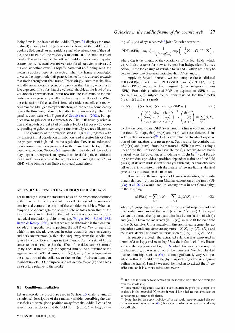
Galaxies in the saddle frame of the cosmic web 27
locity flow in the frame of the saddle. Figure F1 displays the (nor-malized) velocity field of galaxies in the frame of the saddle whiletracking (left panel) or not (middle panel) the orientation of the sad-dle, and the PDF of the velocity’s modulus and orientation (rightpanel). The velocities of the left and middle panels are computedas previously, i.e. as an average velocity for all galaxies in given 2Dbin and smoothed over 0.3 Mpc/h. Note that no flipping w.r.t. thez-axis is applied here. As expected, when the frame is orientatedtowards the larger node (left panel), the net flow is directed towardsthat node throughout that frame. Interestingly, note that the flowactually overshoots the peak of density in that frame, which is infact expected, in so far that the velocity should, at the level of theZel’dovich approximation, point towards the minimum of the po-tential, whose peak is typically further away from the saddle. Whenthe orientation of the saddle is ignored (middle panel), one recov-ers a ‘saddle-like’ geometry for the flow, i.e. the saddle point locallyrepels the flow longitudinally but attracts it transversally. The rightpanel is consistent with Figure 6 of Sousbie et al. (2008), but ap-plies now to galaxies in HORIZON-AGN. The PDF velocity orienta-tion and moduli present a tail of high velocities (at cos δ < 0), cor-responding to galaxies converging transversally towards filaments.
The geometry of the flow displayed in Figure F1, together withthe distinct initial population distribution (and accretion history) forthe progenitor of high and low mass galaxies allow us to understandtheir cosmic evolution presented in the main text. On top of thispassive advection, Section 6.5 argues that the tides of the saddlemay impact directly dark halo growth while shifting the conditionalmean and co-variances of the accretion rate, and galactic V/σ orsSFR while biasing spin (hence cold gas) acquisition.
APPENDIX G: STATISTICAL ORIGIN OF RESIDUALS
Let us finally discuss the statistical basis of the procedure describedin the main text to study second order effects beyond the mass anddensity and capture the origin of these hidden variables. When at-tempting to disentangle the specific role of tides from that of thelocal density and/or that of the dark halo mass, we are facing astatistical mediation problem (see e.g. Wright 1934; Sobel 1982;Baron & Kenny 1986), in that we aim to determine if the tidal ten-sor plays a specific role impacting the sSFR (or V/σ or age etc.)which is not already encoded in other quantities such as densityand dark matter mass (which also vary away from the saddle, buttypically with different maps in that frame). For the sake of beingconcrete, let us assume that the effect of the tides can be summedup by a scalar field α (e.g. the squared sum of the difference of theeigenvalues of the Tidal tensor, α =
∑(λi−λj)2, which quantifies
the anisotropy of the collapse, or the net flux of advected angularmomentum, etc.). Our purpose is to extract the map α(r) and checkits structure relative to the saddle.
G1 Conditional mediation
Let us motivate the procedure used in Section 6.5 while relying ona statistical description of the random variables describing the var-ious fields at some given position away from the saddle. Let us firstassume for simplicity that the field X = (sSFR, δ ≡ log ρ,m ≡
logMDH, α) obeys a centred21 joint Gaussian statistics:
PDF(sSFR, δ,m, α)=1√
det(C0)exp
(−1
2XT ·C0
−1 ·X),
where C0 is the matrix of the covariance of the four fields, whichwe will also assume for now to be position independent (but seebelow). Note the change of variable to m and δ which are likely tobehave more like Gaussian variables than MDM and ρ.
Applying Bayes’ theorem, we can compute the conditionalPDF(sSFR|δ,m, α) = PDF(sSFR, δ,m, α)/PDF(δ,m, α),where PDF(δ,m, α) is the marginal (after integration oversSFR). From this conditional PDF the expectation sSFR(r) ≡〈sSFR|δ,m, α, r〉 subject to the constraint of the three fieldsδ(r),m(r) and α(r) reads
sSFR(r) =(〈sSFR δ〉, 〈sSFRm〉, 〈sSFRα〉
)(G1)
·
〈δ2〉 〈δm〉 〈δα〉〈δm〉 〈m2〉 〈αm〉〈δα〉 〈αm〉 〈α2〉
−1
·
δ(r)m(r)α(r)
≡∑i>1
βiXi,
so that the conditional sSFR(r) is simply a linear combination ofthe three Xi maps, δ(r), m(r) and α(r) (with coefficients βi in-volving the covariances)22. Let us now take the statistical expecta-tion of this equation at a given pixel. Subtracting the contributionof 〈δ(r)〉 and 〈m(r)〉 from the measured 〈sSFR(r)〉 (while using alinear fit to the simulation to estimate the βi since we do not knowa priori what the covariances involving α might be23) and focus-ing on residuals provides a position-dependent estimate of the field〈α(r)〉. If its amplitude is statistically significant, its geometry maytell us if it is consistent with the nature of the mediating physicalprocess, as discussed in the main text.
If we relaxed the assumption of Gaussian statistics, the condi-tionals derived from an Gram-Charlier expansion of the joint PDF(Gay et al. 2012) would lead (to leading order in non Gaussianity)to the mapping
sSFR(r) =∑i>1
βiXi +∑i,j>1
βijXiXj + · · · (G2)
where βi (resp. βij) are functions of the second resp. second andthird order cumulants of the fields (such as 〈δ2α〉 etc). Once againwe could subtract the (up to quadratic) fitted contribution of 〈δ(r)〉and 〈m(r)〉 from the measured 〈sSFR(r)〉 so as to fit the manifoldof the X samples. Unfortunately, in this non-linear regime, the ex-pectations would not compute any more, 〈XiXj〉 6= 〈Xi〉〈Xj〉 andthe residuals will also involve terms such as 〈δα〉, 〈mα〉 or 〈α2〉.
In practice though, the extracted relationships expressed interms of δ = log ρ and m = logMDH do in fact look fairly linear,see e.g. the top panels of Figure 16, which favours the assumptionof Gaussianity, as was assumed in the main text. We also checkedthat relationships such as (G1) did not significantly vary with po-sition within the saddle frame (by marginalising over sub regionswithin the frame). Finally we used the median to extract the βi co-efficients, as it is a more robust estimator.
21 the PDF is assumed to be centred on the mean value of the field averagedover the whole map22 This relationship could have also been obtained by principal componentanalysis in the extended X space: it would have led to the same sets ofcovariances as linear coefficients.23 Note that for an explicit choice of α we could have extracted the co-variances entering equation (G1) from the simulation and estimated the βiaccordingly.
MNRAS 000, 000–000 (0000)

28 K. Kraljic, C. Pichon, Y. Dubois, S. Codis et al.
−2 −1 0 1 2y [Mpc/h]
−3
−2
−1
0
1
2
3
4
z[M
pc/h]
9.00≤ logM⋆ ≤ 11.99
0.00
0.15
0.30
0.45
0.60
0.75
0.90
cosθ
−1.0 −0.5 0.0 0.5 1.0cos δ
100
200
300
400
500
600
700
v[km/s]
9.00≤ logM⋆ ≤ 11.99
0.0004
0.0012
0.002
0.0028
−2 −1 0 1 2y [Mpc/h]
−3
−2
−1
0
1
2
3
4
z[M
pc/h]
9.00≤ logM⋆ ≤ 11.99
−0.8
−0.6
−0.4
−0.2
0.0
0.2
0.4
0.6
0.8
cosθ
Figure F1. Left and middle panels: Velocity vector of galaxies in the frame of the saddle for masses in the range 109 to 1012M at redshift zero, in thelongitudinal plane of the saddle, with the upward direction defined to be towards the node of highest density (left), and without imposing any condition on thedirection of the filament at the saddle (middle). The arrows represent the unitary velocity vector in the y − z plane, colour-coded by the cosine of the anglebetween this vector and the z−axis. Note that as the modulus of the velocity near the saddle point is low, the direction of the velocity vector is not very wellconstrained there. Note also that the structure of the velocity field in the saddle frame is intrinsically complex due to the relative velocity of a saddle w.r.t. thenodes. The grey contours represent the galaxy number counts. Right panel: Probability distribution function of the velocity field of galaxies within the cosmicweb as a function of its modulus v, and the cosine of its angle δ with the closest filament. The excess of galaxies with cos δ close to unity shows that the bulkof the population appears to be flowing along the filaments in the direction of nodes, i.e. the high density regions.
As a word of caution, it should nevertheless be stressed thatsince we are aiming to extract a secondary effect (beyond mass anddensity), the impact of departure from our assumptions may proveto be of the same order as the sought signal. Eventually, larger sta-tistical samples may allow us to statistically disentangle more ro-bustly the various processes. Note finally that carrying out the anal-ysis at fixed stellar mass allows us to avoid the bimodality of somephysical parameters which would clearly have broken the assump-tion of joint Gaussian statistics.
G2 Mediation of multiple causes
An alternative strategy to address the fact that more than one vari-able impact V/σ (and/or sSFR, age etc.) is to sample over narrowbins of stellar and dark halo mass, local density and position rwithin the frame of the cosmic web, and estimate the full joint PDF.This is challenging for a sample of only 105 galaxies, hence canonly be applied to relatively large bins in practice. We attempted todisentangle halo mass, density and tidal effects by computing theresiduals of V/σ (and/or sSFR, age) from median halo mass map-ping in a given stellar mass and density bin. We found comparableresiduals to those shown in Figure 16. However, given the size ofthe bins we use, we cannot draw any definitive conclusions here.Simulations with more statistics should be able to address this dif-ficult point in the future.
MNRAS 000, 000–000 (0000)