generalized regression trees statistica sinica 1995, v. 5 ...loh/treeprogs/guide/grapes.pdf ·...
TRANSCRIPT

Generalized Regression Trees
(Statistica Sinica 1995, v. 5, pp. 641–666)
Probal Chaudhuri Wen-Da Lo Wei-Yin Loh Ching-Ching Yang
Indian Statistical Institute, Calcutta, Chung Cheng Institute of Technology, Taiwan,University of Wisconsin, Madison, and Feng Chia University, Taiwan
Abstract
A method of generalized regression that blends tree-structured nonparametric regression andadaptive recursive partitioning with maximum likelihood estimation is studied. The functionestimate is a piecewise polynomial, with the pieces determined by the terminal nodes of a binarydecision tree. The decision tree is constructed by recursively partitioning the data according tothe signs of the residuals from a model fitted by maximum likelihood to each node. Algorithmsfor tree-structured Poisson and logistic regression and examples to illustrate them are given.Large-sample properties of the estimates are derived under appropriate regularity conditions.
Key words and phrases: Anscombe residual, consistency, generalized linear model, maximumlikelihood, pseudo residual, recursive partitioning, Vapnik-Chervonenkis class.
1 Introduction: motivation and main ideas
Consider a general regression setup in which a real-valued response Y is related to a real or a vector-valued regressor X through a probability model that characterizes the nature of the dependence ofY on X. Let f{y|g(x)} denote the conditional density or mass function of Y given X = x, wherethe form of f is known but g is an unknown function to be estimated. Familiar examples include thelogistic regression model (where Y is binary, and g(x) is the “logit” of the conditional probabilityparameter given X = x), the Poisson regression model (where Y is a nonnegative integer-valuedrandom variable with a Poisson distribution, and g(x) is related to its unknown conditional meangiven X = x), and generalized linear models (GLM) (Nelder and Wedderburn 1972, McCullagh andNelder 1989), where g is related to the link function. On the other hand, g(x) may be the unknownlocation parameter associated with the conditional distribution of Y given X = x. That is, Y maysatisfy the equation Y = g(X) + ε, where the conditional distribution of ε may be normal, Cauchyor exponential power (see, e.g., Box and Tiao 1973) with center at zero.
We focus on the situation where no finite-dimensional parametric model is imposed on g, and it isassumed to be a fairly smooth function. Nonparametric estimation of the functional parameter g hasbeen explored by Chaudhuri and Dewanji (1995), Cox and O’Sullivan (1990), Gu (1990), Hastie andTibshirani (1986, 1990), O’Sullivan, Yandell and Raynor (1986), Staniswalis (1989), Stone (1986,1991a), and others, who considered nonparametric smoothers when the conditional distribution ofthe response given the regressor is assumed to have a known shape (e.g., the conditional distributionmay possess a GLM-type exponential structure).
In the case of the usual regression setup, where Y = g(X)+ε with E(ε|X) = 0, several attemptshave been made to estimate g by recursively partitioning the regressor space and then constructing
1
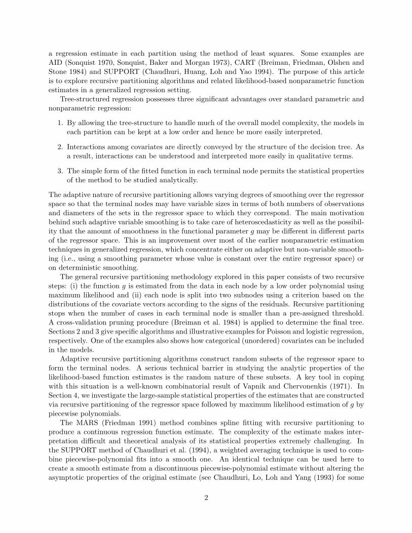
a regression estimate in each partition using the method of least squares. Some examples areAID (Sonquist 1970, Sonquist, Baker and Morgan 1973), CART (Breiman, Friedman, Olshen andStone 1984) and SUPPORT (Chaudhuri, Huang, Loh and Yao 1994). The purpose of this articleis to explore recursive partitioning algorithms and related likelihood-based nonparametric functionestimates in a generalized regression setting.
Tree-structured regression possesses three significant advantages over standard parametric andnonparametric regression:
1. By allowing the tree-structure to handle much of the overall model complexity, the models ineach partition can be kept at a low order and hence be more easily interpreted.
2. Interactions among covariates are directly conveyed by the structure of the decision tree. Asa result, interactions can be understood and interpreted more easily in qualitative terms.
3. The simple form of the fitted function in each terminal node permits the statistical propertiesof the method to be studied analytically.
The adaptive nature of recursive partitioning allows varying degrees of smoothing over the regressorspace so that the terminal nodes may have variable sizes in terms of both numbers of observationsand diameters of the sets in the regressor space to which they correspond. The main motivationbehind such adaptive variable smoothing is to take care of heteroscedasticity as well as the possibil-ity that the amount of smoothness in the functional parameter g may be different in different partsof the regressor space. This is an improvement over most of the earlier nonparametric estimationtechniques in generalized regression, which concentrate either on adaptive but non-variable smooth-ing (i.e., using a smoothing parameter whose value is constant over the entire regressor space) oron deterministic smoothing.
The general recursive partitioning methodology explored in this paper consists of two recursivesteps: (i) the function g is estimated from the data in each node by a low order polynomial usingmaximum likelihood and (ii) each node is split into two subnodes using a criterion based on thedistributions of the covariate vectors according to the signs of the residuals. Recursive partitioningstops when the number of cases in each terminal node is smaller than a pre-assigned threshold.A cross-validation pruning procedure (Breiman et al. 1984) is applied to determine the final tree.Sections 2 and 3 give specific algorithms and illustrative examples for Poisson and logistic regression,respectively. One of the examples also shows how categorical (unordered) covariates can be includedin the models.
Adaptive recursive partitioning algorithms construct random subsets of the regressor space toform the terminal nodes. A serious technical barrier in studying the analytic properties of thelikelihood-based function estimates is the random nature of these subsets. A key tool in copingwith this situation is a well-known combinatorial result of Vapnik and Chervonenkis (1971). InSection 4, we investigate the large-sample statistical properties of the estimates that are constructedvia recursive partitioning of the regressor space followed by maximum likelihood estimation of g bypiecewise polynomials.
The MARS (Friedman 1991) method combines spline fitting with recursive partitioning toproduce a continuous regression function estimate. The complexity of the estimate makes inter-pretation difficult and theoretical analysis of its statistical properties extremely challenging. Inthe SUPPORT method of Chaudhuri et al. (1994), a weighted averaging technique is used to com-bine piecewise-polynomial fits into a smooth one. An identical technique can be used here tocreate a smooth estimate from a discontinuous piecewise-polynomial estimate without altering theasymptotic properties of the original estimate (see Chaudhuri, Lo, Loh and Yang (1993) for some
2

examples). Proposals for extending MARS to logistic regression and GLM-type problems are givenin Friedman (1991), Buja, Duffy, Hastie and Tibshirani (1991) and Stone (1991b). Our approachis more general as it is applicable to other regression setups in addition to logistic regression.
2 Poisson regression trees
Our algorithm for fitting Poisson regression trees has three main components: (i) a method toselect the variable and the splitting value to be used at a partition, (ii) a method to determine thesize of the tree, and (iii) a method to fit a model to each terminal node. Although there are manyreasonable solutions for each component (see Yang (1993) for some variations), the model fittingfor the examples in this section is carried out recursively as follows.
1. The Poisson loglinear model, log(m) = β0 +∑K
k=1 βkxk, is fitted to the data in node t. Herem = EY and x1, . . . , xK are the K covariates.
2. Let mi be the estimated value of m for the ith case and let yi denote the observed value ofYi. The adjusted Anscombe residual (Pierce and Schafer 1986)
ri = {y2/3i − (m2/3
i − (1/9)m−1/3i )}/{(2/3)m1/6
i } (1)
is calculated for each yi in t.
3. Observations with nonnegative ri are classified as belonging to one group and the remainderto a second group.
4. Two-sample t-statistics to test for differences in means and variances between the two groupsalong each covariate axis are computed. The latter test is Levene’s (1960) test.
5. The covariate selected to split the node is the one with the largest absolute t-statistic. Thecut-point for the selected covariate is the average of the two group means along the covariate.Observations with covariate values less than or equal to the cut-point are channeled to theleft subnode and the remainder to the right subnode.
6. After a large tree is constructed, a nested sequence of subtrees is obtained by progressivelydeleting branches according to the pruning method of Breiman et al. (1984), with residualdeviance replacing apparent error in the cost-complexity function.
7. The subtree with the smallest cross-validation estimate of deviance is selected.
Remark 1. Our split selection strategy is motivated by the methods in Chaudhuri et al. (1994)for tree-structured least squares regression and Ahn and Loh (1994) for tree-structured proportionalhazards regression. It differs fundamentally from the exhaustive search strategy used in the AIDand CART algorithms. The latter strategy calls for all possible splits of the data in a node to beevaluated to find the one that most reduces some measure of node impurity (e.g., deviance). Inthe present problem, this requires Poisson loglinear models to be fitted to the subnodes inducedby every split. Because loglinear fitting typically involves Newton-Raphson iteration, this strategyis not practical for routine application on present-day workstations. Our split selection strategyperforms model fitting only once at each node. The task of finding the best split is reduced toa classification problem by grouping the covariate vectors into two classes according to the signsof the residuals. The t-tests, which were developed for tree-structured classification in Loh and
3

Table 1: Coefficients from two Poisson loglinear models fitted to NNM data
Model Term Coefficient t-valueFirst- Intercept 1.71862 23.64degree Dose 0.02556 26.75GLM Time 0.00122 7.74Second- Intercept -1.529E+00 -4.71degree Dose 4.251E-02 4.43GLM Time 1.308E-02 8.73
Dose-squared -4.547E-04 -7.76Time-squared -1.150E-05 -7.12Dose × Time 2.712E-04 10.14
Vanichsetakul (1988), essentially rank the covariates in terms of the degree of clustering of thesigns. The highest ranking covariate is interpreted as the direction in which lack of model fit isgreatest and is selected to split the node.
Remark 2. Empirical evidence (Yang 1993) suggests that the adjusted Anscombe residualsdefined in (1) tend to yield superior splits compared to the unadjusted Anscombe residuals, es-pecially when some of the Poisson means are small. The Pearson and deviance residuals are notemployed because they have the same signs as the unadjusted Anscombe residuals.
We now give two examples to illustrate the Poisson regression tree method. The first exampleuses ordered covariates and the second example categorical (unordered) covariates.
2.1 Effect of N-nitrosomorpholine (NNM) on rats
The data come from an experiment (Moolgavkar, Luebeck, de Gunst, Port and Schwarz 1990) inwhich 173 female rats were exposed to a chemical, N -nitrosomorpholine, at various doses (0, 0.1, 1,5, 10, 20, 40, 80ppm) in their drinking water starting at 14 weeks of age. The animals were killed atdifferent ages and three sections from the identical lobe of the liver were examined for the numberof ATPase-deficient transections. The response is the number of transections, which ranged from 0to 160. These transections, sometimes called foci, are believed to represent clones of premalignantcells. The time to sacrifice ranged from 42 to 686 days.
Table 1 gives the results from fitting a first-degree and then a full second-degree Poisson loglinearmodel to the data. The residual deviances for the two models are 3,455 and 2,027 with 170 and 167degrees of freedom, respectively. Clearly, the first-degree model is rejected in favor of the second-degree model. Notice that the coefficients for dose-squared and time-squared are negative and thatthe most significant term is the interaction between dose and time. This makes interpretationtricky.
The tree in Figure 1 shows the result of fitting piecewise Poisson loglinear models with theproposed method using only main effect terms. The presence of the dose-time interaction is obviousfrom the splits. The tree has five terminal nodes and its residual deviance is 1,432. The samplemean number of transections is given beside each terminal node. This increases from 0.9 when bothdose and time are small to 29.8 when both covariates take large values. The regression coefficientsand t-statistics for the models at the terminal nodes are given in Table 2. The coefficients for doseand time are all positive as expected. Except at node 8, both covariates are highly statistically
4

Dose ≤ 15.1 1����
Time ≤ 413.4 2����
Dose ≤ 4.2 4����
0.9 8
34
����� T
TTTT
15.0 9
32
����� A
AAAA
7.9 5
58
,,
,,
,, ll
ll
llTime ≤ 191.3 3��
��
26.9 6
18
����� T
TTTT
29.8 7
31
Figure 1: Poisson regression tree for NNM data using 10-fold cross-validation. A case goes to theleft subnode if the condition at the split is true. The number beneath a terminal node is the learningsample size. The number on the left of a terminal is the sample mean number of transections.
Table 2: Estimated coefficients and t-values for models in terminal nodes in Figure 1.
Node Intercept Dose Time Residualno. Coef. t Coef. t Coef. t deviance Df5 -1.970 -4.3 0.537 14.6 0.0062 8.5 479 556 -3.377 -8.1 0.039 13.5 0.0282 16.2 86 157 -0.231 -0.9 0.051 12.8 0.0093 14.2 629 288 -2.352 -2.9 1.519 3.8 0.0049 2.1 69 319 -2.439 -7.8 0.112 5.8 0.0146 20.4 168 29
significant. Since the nearest dose to 5ppm in the experiment was 1ppm, this implies that thenumber of transections is essentially random if the dose level is 1ppm or lower and sacrifice time isless than 414 days.
Figure 2 shows contour plots of the fitted log-means for the second-degree GLM and tree-structured models with the observed points superimposed. The contours for the tree-structuredmodel are piecewise-linear and they track the shape of the contours from the GLM model. Observethat the data points are concentrated near the left and bottom sides of the plots and that thecontours in the GLM plot increase rapidly in the upper-right corner. Notice also that the contourline for zero log-count in this plot has a U-shape. These are artifacts caused by the quadraticcomponents in the GLM model. The tree-structured model does not have these problems becauseit models the data in a piecewise fashion. The trade-off is lack of smoothness of the fitted surfaceat the partition boundaries.
Qualitatively similar results are obtained when the above analysis is repeated with log(dose +
5

02468101214
16
Dose (ppm)
Tim
e (d
ays)
0 20 40 60 80
020
040
060
0
.
.
..
.
.
.
.
...
.
.. ...
...
.. .. ... ..
... .. ... .. ... . ........... .......
.
...... .. . ... ..
.....
.. ... .
. ....
. ..
..
..
.
...
...
.
.
..
...
.
.
...
. . ....
.
.
.
.... .
..
..
.
.
..
.
.
.
..
.
.
...
.
..
....
...
.. .. ..
...
..
.
.
-2 -2 0 022
46
8
8
10 10
Dose (ppm)T
ime
(day
s)
0 20 40 60 80
020
040
060
0
.
.
..
.
.
.
.
...
.
.. ...
...
.. .. ... ..
... .. ... .. ... . ........... .......
.
...... .. . ... ..
.....
.. ... .
. ....
. ..
..
..
.
...
...
.
.
..
...
.
.
...
. . ....
.
.
.
.... .
..
..
.
.
..
.
.
.
..
.
.
...
.
..
....
...
.. .. ..
...
..
.
.
Figure 2: Contour plots of predicted log-means of number of transections. The left plot is for thesecond-degree GLM with interaction and the right one for the tree-structured model. Dotted linesin the lower plot mark the partitions and observations are indicated by dots.
0.01) instead of dose. All the coefficients except the one for {log(dose+0.01)}2 are highly significantwhen a second-degree GLM model is fitted to the entire data set. The corresponding Poissonregression tree has the same number of terminal nodes as before, but with different splits.
2.2 A factorial experiment with categorical covariates
The data come from an unreplicated 3× 2× 4× 10× 3 experiment on wave-soldering of electroniccomponents on printed circuit boards (Comizzoli, Landwehr and Sinclair 1990). There are 720observations and the covariates are all categorical variables. The factor levels are:
1. Opening: amount of clearance around a mounting pad (levels ‘small’, ‘medium’, or ‘large’)
2. Solder: amount of solder (levels ‘thin’ and ‘thick’)
3. Mask: type and thickness of the material for the solder mask (levels A1.5, A3, B3, and B6)
4. PadType: geometry and size of the mounting pad (levels W4, D4, L4, D6, L6, D7, L7, L8,W9, and L9)
5. Panel: each board was divided into three panels (levels 1, 2, and 3)
The response is the number of solder skips which range from 0–48.Table 3 gives the results from fitting a Poisson loglinear model to the data with all two-factor
interactions. The three most significant two-factor interactions are between Opening, Solder, andMask. These variables also have the most significant main effects. Chambers and Hastie (1992, p.
6

Table 3: Results from a full second-degree Poisson loglinear model fitted to solder data
Term Df Sum of Sq Mean Sq F -value Pr(F )Opening 2 1587.563 793.7813 568.65 0.00000Solder 1 515.763 515.7627 369.48 0.00000Mask 3 1250.526 416.8420 298.62 0.00000PadType 9 454.624 50.5138 36.19 0.00000Panel 2 62.918 31.4589 22.54 0.00000Opening:Solder 2 22.325 11.1625 8.00 0.00037Opening:Mask 6 66.230 11.0383 7.91 0.00000Opening:PadType 18 45.769 2.5427 1.82 0.01997Opening:Panel 4 10.592 2.6479 1.90 0.10940Solder:Mask 3 50.573 16.8578 12.08 0.00000Solder:PadType 9 43.646 4.8495 3.47 0.00034Solder:Panel 2 5.945 2.9726 2.13 0.11978Mask:PadType 27 59.638 2.2088 1.58 0.03196Mask:Panel 6 20.758 3.4596 2.48 0.02238PadType:Panel 18 13.615 0.7564 0.54 0.93814Residuals 607 847.313 1.3959
10) (see also Hastie and Pregibon (1992, p. 217)) analyze these data and conclude that a parsimo-nious model is one containing all main effect terms and these three two-factor interactions. Theresidual deviance for the latter model is 972 with 691 degrees of freedom (the null deviance is 6,856with 719 degrees of freedom). Estimates of the individual terms in this model are given in Table 4.The model is very complicated and is not easy to interpret.
To confirm the inadequacy of a main-effects model, we fit a Poisson regression tree to thesedata using only main effects models in each node. Because the covariates are categorical, we needto convert them to ordered variables before using the algorithm. Instead of arbitrarily assigningscores, we use a loglinear model to determine the scores as follows. Let X be a categorical variablewith values in the set {1, 2, . . . , c}.
1. Define dummy variables Z1, . . . , Zc−1 such that
Zk =
{1 if X = k0 if X 6= k
k = 1, . . . , c− 1.
2. Fit the Poisson loglinear model, log(m) = γ0+γ1Z1+· · ·+γc−1Zc−1, and let γi (i = 0, . . . , c−1)denote the estimated coefficients.
3. Transform X to the ordered variable V , where
V =
{γ0 + γk if X = k and k 6= cγ0 if X = c.
4. Use the variable V in place of X in the main algorithm.
7

Table 4: Estimates from a Poisson loglinear model fitted to solder data. The model contains allmain effects and all two-factor interactions involving Opening, Solder, and Mask. The letters ‘L’and ‘Q’ below refer to the linear and quadratic components of the Opening factor.
Term Value t
Intercept 0.5219 12.28Opening.L -1.6244 -24.68Opening.Q 0.4573 6.93Solder -1.0894 -20.83Mask1 0.3110 4.47Mask2 0.3834 13.07Mask3 0.4192 28.11PadType1 0.0550 1.66PadType2 0.1058 6.10PadType3 -0.1049 -6.92PadType4 -0.1229 -9.03PadType5 0.0131 1.48PadType6 -0.0466 -5.28PadType7 -0.0076 -1.09PadType8 -0.1355 -12.79PadType9 -0.0283 -4.31Panel1 0.1668 7.93Panel2 0.0292 2.49Opening.LSolder -0.3808 -5.19Opening.QSolder -0.2607 -3.63Opening.LMask1 0.0308 0.32Opening.QMask1 -0.3510 -3.45Opening.LMask2 0.0524 1.28Opening.QMask2 0.2024 4.26Opening.LMask3 0.0871 4.07Opening.QMask3 -0.0187 -0.80SolderMask1 0.0120 0.16SolderMask2 0.1858 6.10SolderMask3 0.1008 6.25
8

Table 5: Covariate V -scores for solder data
Covariate Opening MaskCategory Small Medium Large A1.5 A3 B3 B6V -score 11.071 2.158 1.667 1.611 2.472 5.361 10.417Covariate Panel SolderCategory 1 2 3 Thin ThickV -score 4.042 5.642 5.213 7.450 2.481Covariate Pad typeCategory W4 D4 L4 D6 L6 D7 L7 L8 W9 L9V -score 5.972 6.667 8.667 4.611 3.417 6.042 4.083 5.083 1.583 3.528
Table 6: Estimated coefficients for loglinear models in terminal nodes of tree in Figure 3
Covariate Node 4 Node 5 Node 6 Node 8 Node 9Coef. t Coef. t Coef. t Coef. t Coef. t
Intercept -4.674 -4.93 -3.036 -9.10 -3.910 -8.67 -0.997 -2.21 0.753 3.23Opening 0.139 6.38 0.226 23.33 0.210 1.38 - - - -Mask 0.542 2.38 0.136 9.11 0.223 20.38 0.358 3.33 0.090 8.54Pad type 0.257 5.15 0.212 11.42 0.226 11.65 0.209 8.76 0.166 12.29Panel 0.152 1.05 0.122 2.25 0.389 6.42 0.241 3.38 0.169 4.27
This method of scoring is similar in concept to the method of dealing with categorical covariatesin the FACT method (Loh and Vanichsetakul 1988) for tree-structured classification, although inthe latter the scoring is done at each node instead of merely at the root node; a future version ofthe present algorithm will perform scoring at every node.
The V -scores for each covariate are given in Table 5. Notice that for the variable Opening,the score assigned to the ‘small’ category is much larger than those assigned to the ‘medium’ and‘large’ categories. This suggests that the response is likely to be quite a bit larger when Opening issmall than when it is medium or large. Similarly, the scores for Mask when it takes values B3 orB6 are much larger than for other values.
Figure 3 shows the Poisson regression tree. It has a residual deviance of 1,025. The splitsare on Solder, Mask and Opening, indicating substantial interactions among these covariates. Thesample mean response is given beside each terminal node of the tree. These numbers show thatthe response is least when the Solder amount is thick and the Mask is A1.5 or A3. It is largestwhen the Solder amount is thin, Opening is small, and the Mask is B3 or B6. These conclusionsare not readily apparent from Tables 3 and 4. Table 6 gives the estimated coefficients for theloglinear models in each terminal node. Because the effect of interactions is modeled in the splits,no interaction terms are needed in the piecewise models.
Figure 4 shows plots of the observed values versus the fitted values from the tree-structuredmodel and from the generalized linear model with all main effects and all two-factor interactionsinvolving Solder, Mask, and Opening. The agreement between two sets of fitted values is quite good
9

Solder = Thick 1����
Mask ∈ {A1.5, A3} 2����
0.6 4
180
����� A
AAAA
4.4 5
180
��
��
��� Z
ZZ
ZZ
ZZOpening ∈ {M,L} 3��
��
3.0 6
240
,,
,,
,, ll
ll
llMask ∈ {A1.5, A3} 7��
��
8.0 8
60
����� T
TTTT
24.8 9
60
Figure 3: Poisson regression tree for solder data using 10-fold cross-validation. A case goes to theleft subnode if the condition at a split is true. The number beneath a terminal node is the learningsample size. The number on the left of a terminal node is the sample mean number of solder skips.
and lends support to our method of scoring categorical variables.
3 Logistic regression trees
The basic algorithm for Poisson regression trees is applicable to logistic regression trees. The onlydifference is that a more careful definition of residual is needed. This is because the 0-1 natureof the response variable Y makes the signs of the Pearson and deviance residuals too variable (Lo(1993) gives some empirical evidence). To reduce the amount of variability, the following additionalsteps are taken at each node to smooth the observed Y -values prior to computation of the residuals.
1. Compute pi, the estimate of pi = P (Yi = 1) from a logistic regression model.
2. Smooth the Y -values using the following nearest-neighbor average method (Fowlkes 1987).Let d(xs, xi) be the Euclidean distance between the standardized (i.e., sample variance one)values of xs and xi and let As be the set of [hn]-nearest neighbors of xs, where h ∈ (0, 1) is afixed smoothing parameter. Define ds = maxxi∈As d(xs, xi). The smoothed estimate (calleda ‘pseudo-observation’) is given by
p∗s =∑
xi∈As
wi,syi
/ ∑xi∈As
wi,s
where wi,s = {1 − (d(xi, xs)/ds)3} is the tricube weight function. This method of smoothingis similar to the LOWESS method of Cleveland (1979) except that a weighted average insteadof a weighted regression is employed.
3. Compute the ‘pseudo-residual,’ r∗i = (p∗i − pi), for each observation. The pseudo-residualreplaces the adjusted Anscombe residual in the Poisson regression tree algorithm.
10

......................................................................................................................................................
.....
.
. ..
.........
.... .
.
.....................................
.
....
............................................................................................
.
.........
......
...... .
.
..
.....
....
.. ....
.....
......
............................................................ .
... ...
..
...
... . ...... ..
......
.............
.....
......
.........
...........................
.
...
...
..
.
..
...
...
. ..
.
.
.
. ..
. ..
.............................. .........
.........
.....
.......
....
..
. ..
. ..
..
..
...
.
.. ..
.... ... ..
...
.
..
. ..
......
......
.......
...
...
..
...........
.
...
....
..
. ..
...
. ..
.
.
.
.
..
..
.
.
.
..
..
.
..
.
.
.
GLM fits
Obs
erve
d
0 10 30 50
010
3050
......................................................................................................................................................
.....
.
. ..
.........
. ... .
.
.....................................
.
....
........................................
....................................................
.
..
................... .
.
..
....
.
....
.. ....
.....
......
............................................................ .
..... .
..
...
... .........
......
.............
..
...
......
.........
....
.......................
.
...
.. .
..
.
..
....
... .
.
.
.
.
. ..
. ..
.......................................
...
.
..........
.......
....
..
. ..
. ..
..
..
...
.
.. ..
......
. ..
..
.
.
..
. ..
. ...
... ...
..
.... ...
...
...
..
.... ...
... .
..
..
....
..
. ..
.... ..
.
.
.
.
..
..
.
.
.
..
..
.
...
.
.
Tree model fits
Obs
erve
d0 10 30 50
010
3050
....................................................................................................................................................... ...
.....
. ........
......
............................................................................................................................................................
.......
..
. ... ..
...
. .....
... ...
............................................................. ... ..
. ..
. ...... ..
. ... ...............
................................
.....................
....
...
..
...
...
...
....
..
. ...
..
.............................. ..............................
.......
..
. ... ..
...
. .....
... . .........
..
...
......
......
.......
......
..
...
......
......
......
.
...
...
..
...
...
.
..
....
..
... .
..
GLM fits
Tre
e m
odel
fits
0 10 30 50
010
3050
Figure 4: Observed versus fitted values for solder example. The GLM model contains all maineffects and all two-factor interactions involving Opening, Solder and Mask.
11

Table 7: Range of values of covariates for breast cancer data
Covariate Minimum MaximumAge 30 83Year 58 69Nodes 0 52
Table 8: Estimated coefficients for two linear logistic models fitted to the breast cancer data
Model 1 (deviance = 328 with 302 df) Model 2 (deviance = 316 with 302 df)Term Coefficient t-value Term Coefficient t-valueConstant 1.862 0.70 Constant 2.617 0.97Age -0.020 -1.57 Age -0.024 -1.89Year 0.010 0.23 Year 0.008 0.19Nodes -0.088 -4.47 log(Nodes + 1) -0.733 -5.76
The value of the smoothing parameter h may be chosen by cross-validation if necessary. Ourexperience shows, however, that a fixed value between 0.3 and 0.4 is often satisfactory. This isbecause the pseudo-observations are used here to provide only a preliminary estimate of p thatdoes not have to be very precise.
3.1 Survival following breast cancer surgery
The data in this example come from a study conducted between 1958 and 1970 at the University ofChicago Billings Hospital on the survival of patients who had undergone surgery for breast cancer.There are 306 observations on each of three covariates: Age of patient at time of surgery, Year (yearof surgery minus 1900), and Nodes (number of positive axillary nodes detected in the patient). Theresponse variable Y is equal to 1 if the patient survived 5 years or more, and is equal to 0 otherwise.Two hundred twenty-five of the cases had Y = 1. Table 7 shows the ranges of values taken by thecovariates.
Table 8 gives the coefficient estimates for two linear logistic models fitted to the data. Theonly difference between the models is that the first uses Nodes as a covariate while the second useslog(Nodes + 1). Only the covariate involving Nodes is significant in either model. The residualdeviances of the models are 328 and 316 respectively, each with 302 degrees of freedom.
Haberman (1976) finds that the model
log(p/(1 − p)) = β0 + β1Age + β2Year + β3Nodes + β4(Nodes)2 + β5Age × Year (2)
fits better than the linear logistic Model 1 of Table 8. The residual deviance of (2) is 314 with 300degrees of freedom. The regression coefficients and t-statistics are given on the left half of Table 9.Except for Nodes which is highly significant, all the other covariates are marginally significant (theBonferroni two-sided t-statistic at the 0.05 simultaneous significance level is 2.58).
Landwehr, Pregibon and Shoemaker (1984) re-analyze these data with the help of graphicaldiagnostics. Their model replaces the linear and squared terms in Nodes in Haberman’s model
12

Table 9: Estimated coefficients for models of Haberman and Landwehr et al.
Haberman (deviance = 314 with 300 df) Landwehr et al. (deviance = 302 with 299 df)Term Coefficient t-value Term Coefficient t-valueConstant 35.931 2.62 Constant 77.831 3.29Age -0.661 -2.62 Age -2.868 -2.91Year -0.528 -2.43 Year -0.596 -2.44Age × Year 0.010 2.54 Age × Year 0.011 2.51Nodes -0.175 -4.57 log(Nodes + 1) -0.756 -5.73(Nodes)2 0.003 2.61 (Age)2 0.039 2.35
(Age)3 -0.000 -2.31
Nodes ≤ 4 1����
2
230
����� B
BBBB3
76
Figure 5: Logistic regression tree for breast cancer data using 10-fold cross-validation. A case goesto the left subnode if the condition at a split is true. The number beneath a terminal node is thelearning sample size.
with the terms log(1+Nodes), (Age)2, and (Age)3. This model has a residual deviance of 302 with299 degrees of freedom. The estimated coefficients are given on the right half of Table 9. Againthe term involving Nodes is highly significant and the other terms are marginally significant.
Using Age, Year, and Nodes as covariates and the smoothing parameter value h = 0.3, ourmethod yields the logistic regression tree in Figure 5. It has only one split, on the covariateNodes. The estimated logistic regression coefficients are given in Table 10. None of the t-statisticsis significant, although that for Nodes is marginally significant in the left subnode. The reasonis that much of the significance of Nodes is captured in the split. The estimated coefficient forNodes changes, however, from the marginally significant value of -0.289 to the non-significant valueof -0.012 as we move from the left subnode to the right subnode. This implies that the survivalprobability decreases as the value of Nodes increases from 0 to 4; for values of Nodes greater than4, survival probability is essentially independent of the covariate.
Figure 6 shows plots of the predicted logit values from the three models. The Haberman andtree models appear to be most similar. Note the outlying point marked by an ‘X’ in each plot. Itrepresents an 83 year-old patient who was operated in 1958, had 2 positive axillary nodes and diedwithin 5 years. The cubic term (Age)3 in the Landwehr et al. (1984) model causes it to predict amuch lower logit value for this case than the other models.
Following Landwehr et al. (1984, p. 69), we plot the estimated survival probability as a functionof Age for the situations when Year = 63 and Nodes = 0 or 20. The results are shown in Figure 7.The non-monotonic shapes of the curves for the Landwehr et al. model are due to the cubic term
13

Table 10: Estimated coefficients for logistic regression tree model in Figure 5
Left subnode (Nodes ≤ 4) Right subnode (Nodes > 4)Term Coefficient t-value Term Coefficient t-valueConstant 2.4509 0.734 Constant 0.5117 0.106Age -0.0199 -1.267 Age -0.0378 -1.528Year 0.0063 0.120 Year 0.0243 0.326Nodes -0.2890 -2.255 Nodes -0.0124 -0.472
.. ..
..
..
..
.
..
.
.
..
.
.
.
.
.
.
.
.
. ... . .
.
.
....
..
.. .
.
.
..
.
.
.
.
.
...
.....
.
...
. ..
.
...
. ....
.
...
.
.....
.
......
.
.. .
.
....
......
..... ...
.
. .......
.
...
.... ...
.
.
..
. .......
..
.... ...
...
.
..
... . .
.
.
....
.
.
..
.
. ...
. ..
.
..
.
.
.. .. . ..
..
.
.
......... .
..
. .
.
....
..
.
.
...
.
..
..
..
.
.
..
.
.
..
..
.. ..
...
.
.
.
.
.
.
.
..
..
.
..
...
.
.
..
.
........
. ...
...
..
.
..
.
.
..
.
.
. ..
.. .
Tree
Hab
erm
an
-4 -2 0 2 4
-4-2
02
4
X
.. ..
..
..
. .
.
..
.
.
..
.
..
.
.
.
.
.
. .....
.
.
.. ..
..
.. ..
.
...
.
..
.
...
.....
.
...
. ..
.
...
. ... .
.
.. .
.
...
..
.
... ...
.
.. .
.
....
......
..... ...
.
. .......
.
...
.... ...
.
.
..
. .......
..
.... ...
...
.
..
... . .
..
....
.
.
..
.
. ..
.
. ..
.
..
.
.
.. .. . ..
..
.
.
......... .
..
. .
.
....
..
.
.
...
.
..
....
.
.
..
.
.
..
.... ....
.
.
.
.
.
..
.
..
..
.. .
...
.
.
..
.
..
...
. ..
. ...
.. .
..
.
..
..
...
.
. ..
...
Landwehr
Hab
erm
an
-4 -2 0 2 4
-4-2
02
4X
.. ..
..
..
..
.
..
.
.
..
.
.
.
.
..
.
.
...
. . .
.
.
.
.
.
.
..
..
.
.
.
..
.
.
.
.
.
...
....
.
.
..
.
. ..
.
..
.
..
....
...
.
.
..
.
.
.
....
..
.
..
.
.
...
.
....
..
.....
...
.
.....
.
..
.
..
.
......
..
..
.
..
.....
.
.
.
..
.....
..
....
... ..
.....
.
.
.
.
..
..
.
.
..
.
.
..
.
.
..
.. .
..
..
.
.
.
........
...
. .
.
....
.
..
.
...
.
.
.
....
.
.
..
.
.
..
..
..
....
.
..
.
.
.
.
.
..
..
.
.
.
.
..
.
.
..
.
........
. ...
.
..
..
.
.. .
.
.. .
.
..
.
.
. .
Tree
Land
weh
r
-4 -2 0 2 4
-4-2
02
4
X
Figure 6: Plots of predicted logit values for breast cancer data according to various models.
14
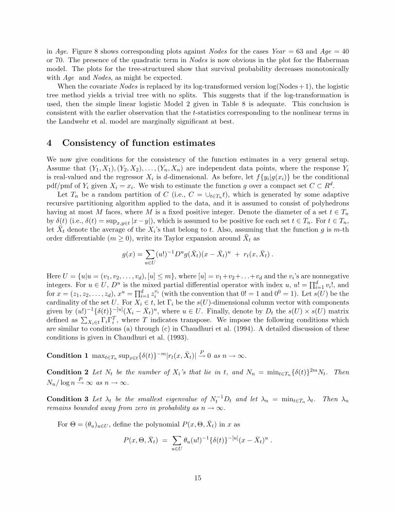
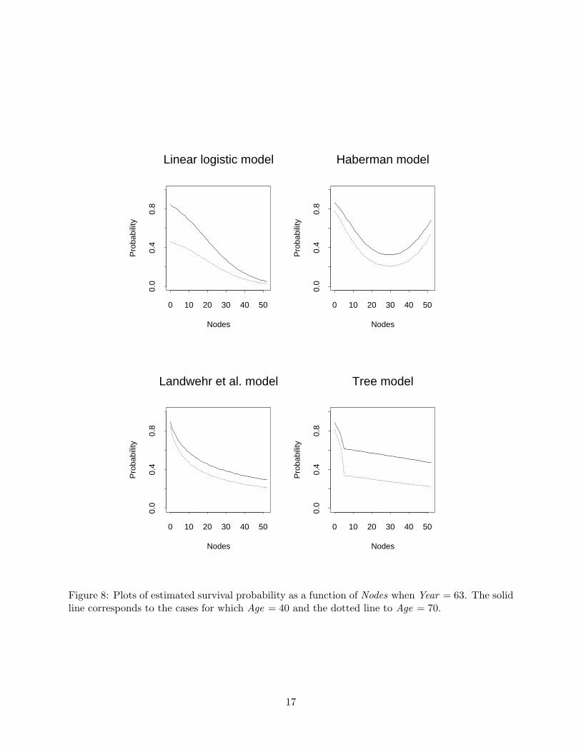
in Age. Figure 8 shows corresponding plots against Nodes for the cases Year = 63 and Age = 40or 70. The presence of the quadratic term in Nodes is now obvious in the plot for the Habermanmodel. The plots for the tree-structured show that survival probability decreases monotonicallywith Age and Nodes, as might be expected.
When the covariate Nodes is replaced by its log-transformed version log(Nodes+1), the logistictree method yields a trivial tree with no splits. This suggests that if the log-transformation isused, then the simple linear logistic Model 2 given in Table 8 is adequate. This conclusion isconsistent with the earlier observation that the t-statistics corresponding to the nonlinear terms inthe Landwehr et al. model are marginally significant at best.
4 Consistency of function estimates
We now give conditions for the consistency of the function estimates in a very general setup.Assume that (Y1, X1), (Y2, X2), . . . , (Yn, Xn) are independent data points, where the response Yi
is real-valued and the regressor Xi is d-dimensional. As before, let f{yi|g(xi)} be the conditionalpdf/pmf of Yi given Xi = xi. We wish to estimate the function g over a compact set C ⊂ Rd.
Let Tn be a random partition of C (i.e., C = ∪t∈Tnt), which is generated by some adaptiverecursive partitioning algorithm applied to the data, and it is assumed to consist of polyhedronshaving at most M faces, where M is a fixed positive integer. Denote the diameter of a set t ∈ Tn
by δ(t) (i.e., δ(t) = supx,y∈t |x−y|), which is assumed to be positive for each set t ∈ Tn. For t ∈ Tn,let Xt denote the average of the Xi’s that belong to t. Also, assuming that the function g is m-thorder differentiable (m ≥ 0), write its Taylor expansion around Xt as
g(x) =∑u∈U
(u!)−1Dug(Xt)(x− Xt)u + rt(x, Xt) .
Here U = {u|u = (v1, v2, . . . , vd), [u] ≤ m}, where [u] = v1+v2+. . .+vd and the vi’s are nonnegativeintegers. For u ∈ U , Du is the mixed partial differential operator with index u, u! =
∏di=1 vi!, and
for x = (z1, z2, . . . , zd), xu =∏d
i=1 zvii (with the convention that 0! = 1 and 00 = 1). Let s(U) be the
cardinality of the set U . For Xi ∈ t, let Γi be the s(U)-dimensional column vector with componentsgiven by (u!)−1{δ(t)}−[u](Xi − Xt)u, where u ∈ U . Finally, denote by Dt the s(U) × s(U) matrixdefined as
∑Xi∈t ΓiΓT
i , where T indicates transpose. We impose the following conditions whichare similar to conditions (a) through (c) in Chaudhuri et al. (1994). A detailed discussion of theseconditions is given in Chaudhuri et al. (1993).
Condition 1 maxt∈Tn supx∈t{δ(t)}−m|rt(x, Xt)| P→ 0 as n→ ∞.
Condition 2 Let Nt be the number of Xi’s that lie in t, and Nn = mint∈Tn{δ(t)}2mNt. ThenNn/ logn P→ ∞ as n→ ∞.
Condition 3 Let λt be the smallest eigenvalue of N−1t Dt and let λn = mint∈Tn λt. Then λn
remains bounded away from zero in probability as n→ ∞.
For Θ = (θu)u∈U , define the polynomial P (x,Θ, Xt) in x as
P (x,Θ, Xt) =∑u∈U
θu(u!)−1{δ(t)}−[u](x− Xt)u .
15

Age
Pro
babi
lity
30 40 50 60 70 80
0.0
0.4
0.8
Linear logistic model
Age
Pro
babi
lity
30 40 50 60 70 800.
00.
40.
8
Haberman model
Age
Pro
babi
lity
30 40 50 60 70 80
0.0
0.4
0.8
Landwehr et al. model
Age
Pro
babi
lity
30 40 50 60 70 80
0.0
0.4
0.8
Tree model
Figure 7: Plots of estimated survival probability as a function of Age when Year = 63. The solidline corresponds to the cases for which Nodes = 0 and the dotted line to Nodes = 20.
16
Nodes
Pro
babi
lity
0 10 20 30 40 50
0.0
0.4
0.8
Linear logistic model
Nodes
Pro
babi
lity
0 10 20 30 40 500.
00.
40.
8
Haberman model
Nodes
Pro
babi
lity
0 10 20 30 40 50
0.0
0.4
0.8
Landwehr et al. model
Nodes
Pro
babi
lity
0 10 20 30 40 50
0.0
0.4
0.8
Tree model
Figure 8: Plots of estimated survival probability as a function of Nodes when Year = 63. The solidline corresponds to the cases for which Age = 40 and the dotted line to Age = 70.
17

Following the estimation procedure described in the previous sections, let Θt be the estimateobtained by applying the maximum likelihood technique to the data points (Yi, Xi) for whichXi ∈ t. In other words,
Θt = arg maxΘ
∏Xi∈t
f{Yi|P (Xi,Θ, Xt)} .
Condition 3 guarantees that for large sample size, each of the matrices Dt’s will be nonsingularand nicely behaved with high probability (cf. Condition (c) in Chaudhuri et al. (1994)). It ensuresregularity in the behavior of the Fisher information matrix associated with the finite-dimensionalmodel fitted to the conditional distribution within each set in Tn. Note that we fit a polynomial ofa fixed degree with a finite number of coefficients to the data points in any set in Tn.
Finally, we need a Cramer-type regularity condition on the conditional distribution of theresponse given the regressor. This condition is crucial in establishing desirable asymptotic behaviorof our estimates, which are constructed using maximum likelihood.
Condition 4 Consider the pdf/pmf f(y|s) as a function of two variables so that s is a real-valuedparameter varying in a bounded open interval J . Here J is such that as x varies over some openset containing C, g(x) takes its values in J . The support of f(y|s) for any given s ∈ J is the same,independent of s. The function log{f(y|s)} is three times continuously differentiable w.r.t. s for anygiven value of y. Let A(y|s), B(y|s) and H(y|s) be the first, second and third derivatives respectivelyof log{f(y|s)} w.r.t. s. Let Y have pdf/pmf f(y|s). The random variable A(Y |s) has zero mean,and the mean of B(Y |s) is negative and stays away from zero as s varies in J . There exists anonnegative function K(y) which dominates each of A(y|s), B(y|s) and H(y|s) for all values ofs ∈ J (i.e., |A(y|s)| ≤ K(y), |B(y|s)| ≤ K(y) and |H(y|s)| ≤ K(y)). The moment generatingfunction of K(Y ), M(w, s) = E [exp{wK(Y )}], remains bounded as w varies over an open intervalaround the origin and s varies over J .
Note that Condition 4 is trivially satisfied when the response Y is binary or, more generally,when its conditional distribution given the regressor is binomial, and s is the logit of the probabilityparameter such that the probability remains bounded away from 0 and 1. This condition holdswhenever the conditional distribution of the response belongs to a standard exponential family(e.g., binomial, Poisson, exponential, gamma, normal, etc.), and s is the natural parameter takingvalues in a bounded interval. If f(y|s) is a location model with s behaving like a location parametervarying over a bounded parameter space, Condition 4 remains true for several important cases suchas the Cauchy or exponential power distribution (see e.g., Box and Tiao (1973)). This conditioncan be viewed as an extension of Condition (d) in Chaudhuri et al. (1994).
Theorem 1 Suppose that Conditions 1 through 4 hold. There is a choice of the maximum likelihoodestimate Θt (possibly a local maximizer of the likelihood) for every t ∈ Tn such that given any u ∈ U ,
maxt∈Tn
supx∈t
|DuP (x, Θt, Xt) −Dug(x)| P→ 0 as n→ ∞.
This theorem guarantees that there is a choice of the maximum likelihood estimate Θt for eacht ∈ Tn so that the resulting piecewise polynomial estimates of the function g and its derivativesare consistent. It may happen that the estimate Θt is only a local maximizer of the likelihoodinstead of being a global maximizer. For instance, the likelihood based on the data points in aset in Tn may have multiple maxima. However, when the conditional distribution of the responsegiven the regressor belongs to a standard exponential family, strict concavity of the loglikelihood
18

guarantees uniqueness of the maximum likelihood estimate in large samples. In the special casewhere a constant (i.e., a polynomial of degree zero) is fitted to the data points in each set in Tn
using the maximum likelihood approach, Theorem 1 generalizes the consistency result for piecewiseconstant tree-structured regression estimates discussed in Breiman et al. (1984).
The piecewise polynomial estimates of g and its derivatives are not continuous everywhere inthe regressor space. Smooth estimates, which can be constructed by combining the polynomialpieces by smooth weighted averaging, will be consistent provided the weight functions are chosenproperly. Theorem 2 in Chaudhuri et al. (1994) describes a way of constructing families of smoothweight functions that give smooth and consistent estimates of g and its derivatives. Some examplesfor smoothing estimates from Poisson and logistic regression trees are given in Chaudhuri et al.(1993).
Remark 3. The results in this section are very general and hence are not specific to anyparticular partitioning algorithm. The main difficulty with applying them to a given algorithm liesin the complexity of algorithmic details such as the choice of splitting rule, pruning method, etc.This is a problem associated with any nontrivial adaptive recursive partitioning algorithm that hasits own particular set of features and tuning parameters. (See page 327 of Breiman et al. (1984)for a discussion of similar issues in the context of tree-structured classification.)
Acknowledgements
The authors are grateful to Dr. Michael Schwarz of the German Cancer Research Center for hispermission to use the NNM data set used in Example 2.1.1. Thanks are also due to Dr. AnupDewanji of Indian Statistical Institute and Dr. Suresh Moolgavkar of Fred Hutchinson CancerResearch Center for their help in making this data set available to the authors.
Chaudhuri’s research was partially supported by a grant from the Indian Statistical Institute.Loh’s research was supported in part by U. S. Army Research Office grants DAAL03-91-G-0111and DAAH04-94-G-0042 and National Science Foundation grant DMS-9304378.
Appendix: proofs
We give a brief sketch of the proof of Theorem 1. More details can be found in Chaudhuri etal. (1993). We begin by giving some preliminary results. Unless stated otherwise, all vectors areassumed to be column vectors. Let Θ∗
t denote the s(U)-dimensional vector with typical entry{δ(t)}[u]Dug(Xt) where u ∈ U . Then P (x,Θ∗
t , Xt) is the Taylor polynomial of g(x) expandedaround Xt.
Lemma 1 Under Conditions 1, 2 and 4, we have
maxt∈Tn
N−1t {δ(t)}−m
∣∣∣∣∣∣∑Xi∈t
[A{Yi|P (Xi,Θ∗
t , Xt)}]Γi
∣∣∣∣∣∣P→ 0 as n→ ∞ .
Proof: First observe that a straightforward application of the mean value theorem of differentialcalculus yields
N−1t {δ(t)}−m
∑Xi∈t
[A{Yi|P (Xi,Θ∗
t , Xt)}]Γi
19
= N−1t {δ(t)}−m
∑Xi∈t
[A{Yi|g(Xi)}] Γi
−N−1t {δ(t)}−m
∑Xi∈t
{rt(Xi, Xt)B(Yi|Zi)}Γi (3)
where Zi is a random variable that lies between P (Xi,Θ∗t , Xt) and g(Xi). Because of Condition 4,
the conditional mean of A{Y |g(X)} given X = x is zero, and if we denote its conditional momentgenerating function by M1(w|x), there exist constants k1 > 0 and ρ1 > 0 such that M1(w|x) ≤2 exp(k1w
2/2) for all x ∈ C and 0 ≤ w ≤ ρ1 (see the arguments at the beginning of Lemma 12.27in Breiman et al. (1984)). Recall that each set in Tn is a polyhedron in Rd having at most Mfaces. The fundamental combinatorial result of Vapnik and Chervonenkis (1971) (Dudley 1978,Section 7) implies that there exists a collection C of subsets of the set {X1, X2, . . . , Xn} such that#(C) ≤ (2n)M(d+2), and for any polyhedron t with at most M faces, there is a set t∗ ∈ C with theproperty that Xi ∈ t if and only if Xi ∈ t∗. By Condition 2 and the arguments used in handlingthe “variance term” in the proof of Theorem 1 in Chaudhuri et al. (1994), it can be shown that
maxt∈Tn
{δ(t)}−mN−1t
∣∣∣∣∣∣∑Xi∈t
[A{Yi|g(Xi)}] Γi
∣∣∣∣∣∣P→ 0 as n→ ∞ .
Further, using Conditions 1, 2 and 4,
maxt∈Tn
N−1t {δ(t)}−m
∣∣∣∣∣∣∑Xi∈t
{rt(Xi, Xt)B(Yi|Zi)
}Γi
∣∣∣∣∣∣≤
[maxt∈Tn
{δ(t)}−m supx∈t
|rt(x, Xt)|]maxt∈Tn
N−1t
∑Xi∈t
K(Yi)|Γi|
P→ 0 as n→ ∞.
This proves the lemma.
Lemma 2 Let γ(t) denote the smallest eigenvalue of the s(U) × s(U) matrix
− N−1t
∑Xi∈t
[B{Yi|P (Xi,Θ∗
t , Xt)}]ΓiΓT
i .
Define γn = mint∈Tn γ(t). Then, under Conditions 1 through 4, γn remains positive and boundedaway from zero in probability as n→ ∞.
Proof: The mean value theorem of differential calculus yields
N−1t
∑Xi∈t
[B{Yi|P (Xi,Θ∗
t , Xt)}]ΓiΓT
i
= N−1t
∑Xi∈t
[B{Yi|g(Xi)} − ψ(Xi)] ΓiΓTi +N−1
t
∑Xi∈t
ψ(Xi)ΓiΓTi
−N−1t
∑Xi∈t
{rt(Xi, Xt)H(Yi|Vi)}ΓiΓTi , (4)
where ψ(x) is the conditional mean of B{Y |g(X)} given X = x, and Vi is a random variable thatfalls between g(Xi) and P (Xi,Θ∗
t , Xt). It follows from Conditions 3 and 4 that if ηn = mint∈Tn η(t),
20
where η(t) is the smallest eigenvalue of the matrix−N−1t
∑Xi∈t ψ(Xi)ΓiΓT
i , then ηn remains positiveand bounded away from zero in probability as n → ∞. On the other hand, the first term on theright of (4) can be handled in the same way as the first term on the right of (3) in the proof ofLemma 1 to yield
maxt∈Tn
N−1t
∣∣∣∣∣∣∑Xi∈t
[B{Yi|g(Xi)} − ψ(Xi)] ΓiΓTi
∣∣∣∣∣∣P→ 0 as n→ ∞ .
Finally, using Conditions 1, 2 and 4, and arguments similar to those employed to treat the secondterm on the right of (3) in the proof of Lemma 1, we obtain the following result for the third termon the right of (4):
maxt∈Tn
N−1t
∣∣∣∣∣∣∑Xi∈t
{rt(Xi, Xt)H(Yi|Vi)}ΓiΓTi
∣∣∣∣∣∣≤
{maxt∈Tn
supx∈t
|rt(x, Xt)|}
maxt∈Tn
N−1t
∑Xi∈t
K(Yi)|ΓiΓTi |
P→ 0 as n→ ∞.
This completes the proof of the lemma.Proof of Theorem 1: First note that the assertion in the Theorem will follow if we show thatthere exist choices for the maximum likelihood estimates Θt’s such that
maxt∈Tn
{δ(t)}−m|Θt − Θ∗t | P→ 0 as n→ ∞ .
For t ∈ Tn, let lt(Θ) denote the loglikelihood based on the observations (Yi, Xi) such that Xi ∈ t.That is, lt(Θ) =
∑Xi∈t log
[f{Yi|P (Xi,Θ, Xt)}
]. Given ρ > 0, define Et(ρ) to be the event:
lt(Θ) is concave in a neighborhood of Θ∗t with radius {δ(t)}mρ (i.e., for Θ satisfying
{δ(t)}−m|Θ − Θ∗t | ≤ ρ), and it has a (possibly local) maximum in the interior of this
neighborhood.
The occurrence of this event implies that the maximum likelihood equation obtained by differenti-ating lt(Θ) w.r.t. Θ will have a root Θt such that {δ(t)}−m|Θt − Θ∗
t | < ρ. A Taylor expansion oflt(Θ) around Θ∗
t yields
lt(Θ) = lt(Θ∗t ) +
∑Xi∈t
(Θ − Θ∗t )
T ΓiA{Yi|P (Xi,Θ∗t , Xt)}
+ (1/2)∑Xi∈t
(Θ − Θ∗t )
T ΓiΓTi B{Yi|P (Xi,Θ∗
t , Xt)}(Θ − Θ∗t )
+ (1/6)∑Xi∈t
{(Θ − Θ∗t )
T Γi}3H(Yi|Wi), (5)
where Wi is a random variable lying between P (Xi,Θ∗t , Xt) and P (Xi,Θ, Xt). For the third term
on the right of (5), note that the Γi’s are bounded vectors. Also, for Θ in a sufficiently smallneighborhood of Θ∗
t , we have∑
Xi∈t |H(Yi|Wi)| ≤ ∑Xi∈tK(Yi) in view of Condition 4. It follows
from Lemmas 1 and 2 and the arguments used in their proofs that there exists ρ3 > 0 such thatwhenever ρ ≤ ρ3, we must have Pr(∩t∈TnEt(ρ)) → 1 as n→ ∞. This proves the theorem.
21

References
Ahn, H. and Loh, W.-Y. (1994). Tree-structured proportional hazards regression modeling, Bio-metrics 50: 471–485.
Box, G. E. P. and Tiao, G. C. (1973). Bayesian Inference in Statistical Analysis, Addison-Wesley,Reading.
Breiman, L., Friedman, J. H., Olshen, R. A. and Stone, C. J. (1984). Classification and RegressionTrees, Wadsworth, Belmont.
Buja, A., Duffy, D., Hastie, T. and Tibshirani, R. (1991). Comment on “Multivariate adaptiveregression splines”, Annals of Statistics 19: 93–99.
Chambers, J. M. and Hastie, T. J. (1992). An appetizer, in J. M. Chambers and T. J. Hastie (eds),Statistical Models in S, Wadsworth & Brooks/Cole, Pacific Grove, pp. 1–12.
Chaudhuri, P. and Dewanji, A. (1995). On a likelihood based approach in nonparametric smoothingand cross-validation, Statistics and Probability Letters 22: 7–15.
Chaudhuri, P., Huang, M.-C., Loh, W.-Y. and Yao, R. (1994). Piecewise-polynomial regressiontrees, Statistica Sinica 4: 143–167.
Chaudhuri, P., Lo, W.-D., Loh, W.-Y. and Yang, C.-C. (1993). Generalized regression trees:Function estimation via recursive partitioning and maximum likelihood, Technical Report 903,University of Wisconsin, Madison, Department of Statistics.
Cleveland, W. S. (1979). Robust locally weighted regression and smoothing scatter plots, Journalof the American Statistical Association 74: 829–836.
Comizzoli, R. B., Landwehr, J. M. and Sinclair, J. D. (1990). Robust materials and processes: Keyto reliability, AT&T Technical Journal 69: 113–128.
Cox, D. D. and O’Sullivan, F. (1990). Asymptotic analysis of penalized likelihood and relatedestimators, Annals of Statistics 18: 1676–1695.
Dudley, R. M. (1978). Central limit theorems for empirical measures, Annals of Probability 6: 899–929. Corr: 7, 909–911.
Fowlkes, E. B. (1987). Some diagnostics for binary logistic regression via smoothing, Biometrika74: 503–515.
Friedman, J. H. (1991). Multivariate adaptive regression splines (with discussion), Annals of Statis-tics 19: 1–67.
Gu, C. (1990). Adaptive spline smoothing in non-Gaussian regression models, Journal of theAmerican Statistical Association 85: 801–807.
Haberman, S. J. (1976). Generalized residuals for log-linear models, Proceedings of the 9th Inter-national Biometrics Conference, Biometric Society, Boston, pp. 104–122.
Hastie, T. J. and Pregibon, D. (1992). Generalized linear models, in J. M. Chambers and T. J.Hastie (eds), Statistical Models in S, Wadsworth & Brooks/Cole, Pacific Grove, pp. 195–248.
22

Hastie, T. J. and Tibshirani, R. J. (1986). Generalized additive models (with discussion), StatisticalScience 1: 297–310.
Hastie, T. J. and Tibshirani, R. J. (1990). Generalized Additive Models, Chapman and Hall, London.
Landwehr, J. M., Pregibon, D. and Shoemaker, A. C. (1984). Graphical methods for assessinglogistic models, Journal of the American Statistical Association 79: 61–83.
Levene, H. (1960). Robust tests for equality of variances, in I. Olkin, S. G. Ghurye, W. Hoeffding,W. G. Madow and H. B. Mann (eds), Contributions to Probability and Statistics, StanfordUniversity Press, Stanford, pp. 278–292.
Lo, W.-D. (1993). Logistic Regression Trees, PhD thesis, University of Wisconsin, Madison.
Loh, W.-Y. and Vanichsetakul, N. (1988). Tree-structured classification via generalized discriminantanalysis (with discussion), Journal of the American Statistical Association 83: 715–728.
McCullagh, P. and Nelder, J. A. (1989). Generalized Linear Models, Chapman and Hall, London.
Moolgavkar, S. H., Luebeck, E. G., de Gunst, M., Port, R. E. and Schwarz, M. (1990). Quantita-tive analysis of enzyme-altered foci in rat hepatocarcinogenesis experiments—I. Single agentregimen, Carcinogenesis 11: 1271–1278.
Nelder, J. A. and Wedderburn, R. W. M. (1972). Generalized linear models, Journal of the RoyalStatistical Society, Series A 135: 370–384.
O’Sullivan, F., Yandell, B. S. and Raynor, W. J. J. (1986). Automatic smoothing of regressionfunctions in generalized linear models, Journal of the American Statistical Association 81: 96–103.
Pierce, D. A. and Schafer, D. W. (1986). Residuals in generalized linear models, Journal of theAmerican Statistical Association 81: 977–986.
Sonquist, J. N. (1970). Multivariate model building, Technical report, Institute for Social Research,University of Michigan.
Sonquist, J. N., Baker, E. L. and Morgan, J. A. (1973). Searching for structure, Technical report,Institute for Social Research, University of Michigan.
Staniswalis, J. G. (1989). The kernel estimate of a regression function in likelihood-based models,Journal of the American Statistical Association 84: 276–283. Corr: 85, 1182.
Stone, C. J. (1986). The dimensionality reduction principle for generalized additive models, Annalsof Statistics 14: 590–606.
Stone, C. J. (1991a). Asymptotics for doubly flexible log-spline response models, Annals of Statistics19: 1832–1854.
Stone, C. J. (1991b). Comment on “Multivariate adaptive regression splines”, Annals of Statistics19: 113–115.
Vapnik, V. N. and Chervonenkis, A. Y. (1971). On the uniform convergence of relative frequenciesof events to their probabilities, Theory of Probability and Its Applications 16: 264–280.
23

Yang, C.-C. (1993). Tree-structured Poisson Regression, PhD thesis, University of Wisconsin,Madison.
24