statistica sinica - arxiv · statistica sinica 1 the restricted consistency property of leave-n...

Statistica Sinica 1

The restricted consistency property of leave-nv-out

cross-validation for high-dimensional variable selection

Yang Feng and Yi Yu

Columbia University and University of Bristol

Abstract: Cross-validation (CV) methods are popular for selecting the tuning pa-

rameter in the high-dimensional variable selection problem. We show the mis-

alignment of the CV is one possible reason of its over-selection behavior. To fix this

issue, we propose a version of leave-nv-out cross-validation (CV(nv)), for selecting

the optimal model among the restricted candidate model set for high-dimensional

generalized linear models. By using the same candidate model sequence and a

proper order of construction sample size nc in each CV split, CV(nv) avoids the

potential hurdles in developing theoretical properties. CV(nv) is shown to enjoy the

restricted model selection consistency property under mild conditions. Extensive

simulations and real data analysis support the theoretical results and demonstrate

the performances of CV(nv) in terms of both model selection and prediction.

Key words and phrases: Leave-nv-out cross-validation; Generalized linear models;

Restricted maximum likelihood estimators; Restricted model selection consistency;

Variable selection.

arX

iv:1

308.

5390

v3 [

stat

.ME

] 1

6 Ja

n 20

18

2 Yang Feng and Yi Yu

1. Introduction

In recent years, massive high-throughput data sets are generated as a result

of technological advancements in many fields. Such data are featured by the large

number of variables p compared with the sample size n. For an overview of the

many challenges associated with high-dimensional statistical modeling, we refer

the readers to Fan and Lv (2010) and Buhlmann and van de Geer (2011).

A crucial goal in high-dimensional data analysis is to achieve a good balance

between the goodness-of-fit and the complexity of the model, as both predictabil-

ity and model interpretability are important to practitioners in many scientific

fields. One popular avenue to achieve this balance is the imposition of penalties

on the model complexity, which leads to simultaneous variable selection and pa-

rameter estimation in one single step. Numerous efforts have been made, from

both theoretical and numerical perspectives; to name but a few, Tibshirani (1996)

proposed Lasso, which is the `1 penalty, or equivalently, Chen and Donoho (1994)

proposed basis pursuit. Also, folded-concave penalties including SCAD (Fan and

Li, 2001) and MCP (Zhang, 2010) have been proposed and widely used over the

years.

One of the important aspects of penalization techniques is the tuning param-

eter, which determines how much penalty is imposed. Over-penalization runs

the risk of overlooking scientifically meaningful information; on the other hand,

under-penalization may erroneously identify seemingly meaningful patterns that

are actually the result of experimental noise. It is, therefore, critical to choose

the tuning parameter with care.

There has been an abundance of research on using certain kind of informa-

tion criteria to select the tuning parameter; these include the generalized cross-

validation (Tibshirani, 1996; Wang et al., 2007), the Cp (Efron et al., 2004),

the extended Bayesian information criterion (EBIC) (Chen and Chen, 2008; Luo

and Chen, 2014), the modified BIC (Wang et al., 2009), the generalized infor-

mation criterion (Zhang et al., 2010; Fan and Tang, 2013), etc. Other related

work includes selection of the tuning parameter through joint estimation of the

regression coefficient and the standard deviation (Stadler et al., 2010; Sun and

Zhang, 2012).

Another popular method for selecting the tuning parameter is cross-validation

Leave-nv-out CV for high-dimensional variable selection 3

(CV), which is a data-driven method. A vast amount of theoretical work has been

done for CV in the fixed-dimensional linear regression models. For example,

leave-one-out CV (CV(1)) is shown to be asymptotically equivalent to Akaike

information criterion (AIC), Cp, jackknife, and bootstrap (Stone, 1977; Efron,

1983, 1986). Shao (1993) proved the model selection inconsistency of CV(1) for

the fixed-dimensional linear regression model. In addition, for leave-nv-out CV

(CV(nv)), the author gave the proper ratio of the size of construction set to

that of validation set which turns out to be necessary for model selection con-

sistency. Here, by construction and validation data sets we mean the subsets

used to construct and validate the estimators in CV splits. However, K-fold

CV, the most commonly used method, is well known for its conservativeness, i.e.

the corresponding estimator selects far too many noise variables (Yu and Feng,

2014b). As mentioned in Zhang and Huang (2008), the theoretical justification

of CV based tuning parameter is unclear for model selection purposes. Yu and

Feng (2014b) proposed the modified cross-validation for high-dimensional linear

regression models and showed that it outperforms the regular K-fold CV in nu-

merical experiments. Compared with Yu and Feng (2014b), in this paper, we

study the leave-nv-out cross-validation for a sequence of candidate models from

the whole data set and developed the restricted consistency results under the

generalized linear model framework for high-dimensional variable selection.

Another related work is relaxed Lasso (Meinshausen, 2007), which is a two-

stage method, with the penalty at the second stage only operating on those

variables being selected at the first stage. The author conjectured that the K-fold

CV for this two-step method will achieve model selection consistency. Different

from Meinshausen (2007), in this paper we study the theoretical behaviors of the

penalties, and mainly focus on the model selection instead of proposing a variant

of Lasso procedure, with rigorous discussions on the asymptotic behavior of CV

provided.

The main contribution of the paper is two-fold: (1) investigations are con-

ducted for the advantages and drawbacks of the commonly used CV methods

for tuning parameter selection in the penalized estimation methods; (2) studying

the leave-nv-out cross-validation, which is shown to be consistent in a restricted

sense for a wide range of penalty functions in the high-dimensional generalized


linear model framework.

We would like to introduce some of the notation used throughout this paper.

For a p-dimensional vector β and an n× p-dimensional matrix A, suppose s is a

subset of {1, · · · , n} and α is a subset of {1, · · · , p}, then βα represents the sub-

vector of β corresponding to α, As represents the submatrix of A corresponding

to rows with indices in s and Aα represents the submatrix of A corresponding to

columns with indices in α. Let |s| represent the cardinality of set s. In addition,

define the `0, `1 and `2 norms of β as ‖β‖0 =∑p

j=1 1{βj 6= 0}, ‖β‖1 =∑p

j=1 |βj |and ‖β‖ = [

∑pj=1 β

2j ]1/2, respectively. Let g1 and g2 be two functions of n. We

use g1(n) = Θ(g2(n)) to represent that they are asymptotically of the same order,

i.e., there exist positive constants c1 and c2, such that

c1 ≤ lim infn

g1(n)/g2(n) ≤ lim supn

g1(n)/g2(n) ≤ c2.

The rest of the paper is organized as follows. We introduce the general-

ized linear model setup and discuss the K-fold CV in Section 2. Motivated by

the issues with the K-fold CV, we introduce the leave-nv-out cross-validation

(CV(nv)) for high-dimensional variable selection, and show CV(nv) can achieve

the restricted model selection consistency in Section 3. We conduct extensive

simulation studies in Section 4 and a real data analysis in Section 5 to compare

CV(nv) with other types of CV methods as well as many state-of-the-art infor-

mation criteria. We conclude the paper with a short discussion in Section 6 while

all the technical details are collected in the Appendix.

2. Model setup and K-fold cross-validation

2.1. Model setup

Suppose we have n i.i.d. observation pairs (xi, yi), i = 1, · · · , n, where xi is

a p-dimensional predictor and yi is the response. For generalized linear models,

we assume the conditional distribution of y given x belongs to an exponential

family with the canonical link and canonical parameter θ = x>β; that is, it has

the following density function,

f(y;x,β) = c(y, φ) exp((yθ − b(θ))/a(φ)),

where φ ∈ (0,∞) is the dispersion parameter, the functions a(·), b(·) and c(·, ·)are known and different for different models. Let βo be the true regression


parameter, with ‖βo‖0 = do. In the high-dimensional setting, p may well exceed

n but do is usually assumed to be strictly upper bounded by n, i.e., do < n.

Up to an affine transformation with θi = x>i β, the log-likelihood divided by the

sample size is given by

`(β) = n−1n∑i=1

{yiθi − b(θi)}. (1.1)

Minimizing the penalized negative log-likelihood function leads to the following

estimator.

β(λ) = arg minβ∈Rp

{−`(β) + pλ,γ(β)}, (1.2)

where pλ,γ(·) is the penalty function.

Given subset s ⊂ {1, · · · , n}, the log-likelihood function evaluated on the

subset s is

`(s)(β) = (|s|)−1∑i∈s{yiθi − b(θi)}. (1.3)

Then the corresponding minimizer of the penalized negative log-likelihood is

β(s)

(λ) = arg minβ∈Rp

{−`(s)(β) + pλ,γ(β)}, (1.4)

In this paper, we only consider separable sparsity-inducing penalties; that

is, there exists a non-negative function ρ(·), such that for any vector β =

(β1, · · · , βp)>, the penalty function pλ,γ(·) satisfies

pλ,γ(β) =

p∑j=1

ρ(|βj |;λ, γ), (1.5)

where λ and γ are the parameters of the penalty function and the minimizer

of the penalized negative log-likelihood leads to a sparse solution. Both convex

and folded-concave penalties can be written in the form of (1.5). For convex

penalties, such as Lasso (Tibshirani, 1996), γ = ∞; while for folded-concave

penalties, 0 < γ <∞. In the penalty function (1.5), γ is a parameter controlling

the concavity of the penalty, and in this paper we only focus on studying the

collection of solutions as λ changes while fixing γ.


S1. Using the whole data, generate a data-driven penalty parameter sequence

λ = {λ1, · · · , λR}. Compute the solution path {βr, r = 1, · · · , R}, where

βr = β(λr).

S2. Randomly divide the data set into K folds, and denote the indices of each fold as

sk, k = 1, · · · ,K, and s(−k) = {1, · · · , n} \ sk.

S3. For each fold k = 1, · · · ,K

(a) Using the construction data in s(−k), generate its own penalty parameter

sequence λ(−k) = {λ(−k)1 , · · · , λ(−k)R }.

(b) Compute the corresponding solution path {β(−k)r , r = 1, · · · , R}, where

β(−k)r = β

(s(−k))(λ

(−k)r ) is the penalized estimator defined in (1.4) with

penalty parameter λ(−k)r .

(c) Evaluate the prediction performance of {β(−k)r , r = 1, · · · , R} on the

validation data in sk using the negative log-likelihood function. The

resulting values are denoted by {Lkr , r = 1, · · · , R}, where

Lkr = −`(sk)(β

(−k)r ) as defined in (1.3).

S4. Calculate the average criterion values {Lr, r = 1, · · · , R} where

Lr = K−1∑K

k=1 Lkr . Output the optimal location r = arg minr=1,...,R Lr along

with its corresponding solution βr.

Algorithm 1: K-fold CV for a typical path algorithm.

A popular class of algorithms on solving (1.2) are called path algorithms.

Many different path algorithms have been proposed, including forward regression,

stepwise regression, lars (Efron et al., 2004), glmpath (Park and Hastie, 2007),

glmnet (Friedman et al., 2010), ncvreg (Breheny and Huang, 2011), apple (Yu

and Feng, 2014a), among others. In a path algorithm, a collection of (usually

sparse) estimators {βr, r = 1, · · · , R} are generated, where R represents the total

number of candidate estimators. Then the natural question is to choose the best

estimate βr among the R candidates according to certain criteria.

2.2. Cross-validation

There are many different versions of CV, to avoid ambiguity, we describe K-

fold CV with glmnet and ncvreg in the penalized negative log-likelihood context

in Algorithm 1.


In Algorithm 1, to compare the performance of {βr, r = 1, · · · , R}, we are

averaging the prediction performance on the corresponding validation set sk over

the K folds using the estimator β(−k)r from the construction set s(−k). How-

ever, there is no guarantee that we are averaging across the same models or the

same tuning parameters across different folds. In path algorithms, the tuning

parameters are determined by the construction data set, and the estimators are

determined by the tuning parameters and the construction data set.

Remark 1. In some other path algorithms including lars and glmpath, instead

of starting with a sequence of data-driven penalty parameters, they proceed by

adaptively adding/deleting one predictor at a time from the model and provide

the corresponding βr after each operation. Note that the solution βr from such

path algorithms would also implies a certain value of λr in (1.2). As a result,

the preceding discussions regarding the averaging process also apply to those

algorithms.

Remark 2. In practice, it is also common to use the tuning parameter sequence λ

generated by the whole data in all splits. Although this guarantees the alignment

of tuning parameters across different splits, this still causes mis-alignment in

terms of model sequences, and this actually could cause more problems due to

the fact that a desirable tuning parameter should be a function of the sample

size. In any case, it would be very difficult to link the chosen tuning parameter

from the splits with its performance in the whole data.

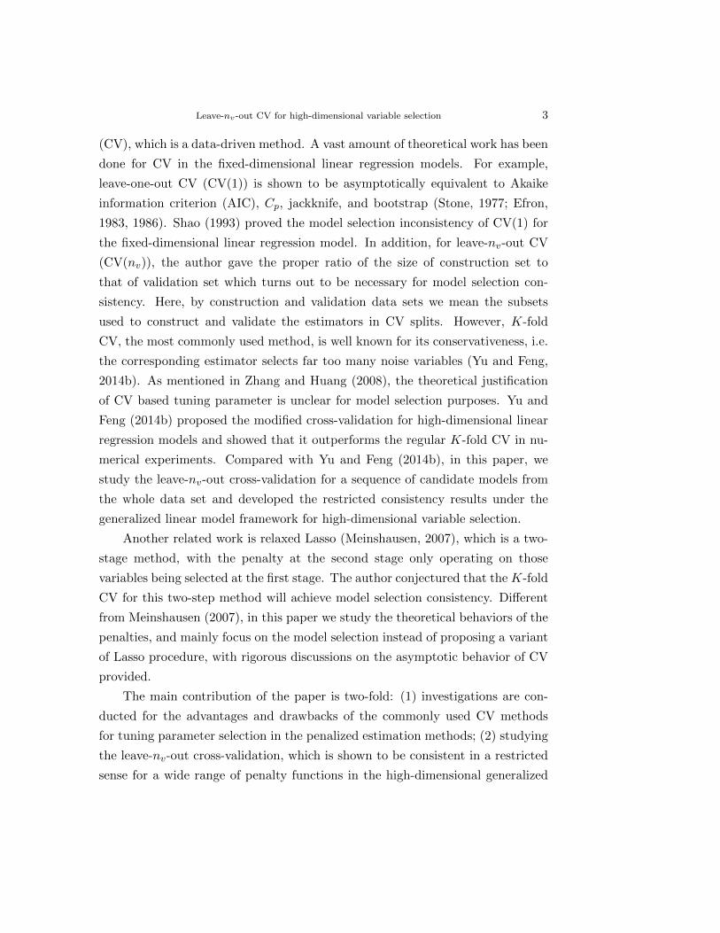
We conduct a simple simulation for a high-dimensional linear regression ex-

ample with the 5-fold CV. In Figure 1, we show the corresponding results of two

different construction data sets when performing the CV. In the left panel we

show the first 30 values of λ on each path, with the x-axis being the location

indices; in the right panel, the sequences of the model sizes are presented against

their locations on the solution paths. The CV averages models across different

splits, but as we can see from Figure 1, the corresponding λ sequences and the

model size sequences are both very different for those two different splits. As a

result, it is very difficult to derive any theoretical justification for either model se-

lection or tuning parameter selection property of the CV tuned estimator. More

numerical results on the alignment issue of the CV will be shown in Section 4.1.


0 5 10 15 20 25 30

0.2

0.3

0.4

0.5

0.6

Location

λ

Subsample 1Subsample 2

0 5 10 15 20 25 30

010

2030

40

LocationM

odel

siz

e

Subsample 1Subsample 2

Figure 1: An example on K-fold cross-validation

3. Leave-nv-out cross-validation

With a better understanding of the issues of the CV in Section 2, we propose a

version of CV(nv) in this section. We first introduce some key concepts regarding

model selection in Section 3.1 and CV(nv), then point out its major differences

from the CV in Section 3.2. In Section 3.3, we show that CV(nv) is restricted

model selection consistent (to be defined formally in Section 3.1) under mild

technical conditions in the generalized linear model framework for both convex

and folded-concave penalties.

3.1. Key concepts

From the solution path {βr, r = 1, · · · , R} in Algorithm 1, one can get

a corresponding path of models A = {αr, r = 1, · · · , R}, where αr = {j ∈{1, · · · , p} : (βr)j 6= 0} is the indices with nonzero coefficient estimates. Similar

to Shao (1993), we divide A into two disjoint subsets: Ac and its complement

A \ Ac, where Ac = {α ∈ A : (Xα)βoα = Xβo}. Here we give three definitions

which constitute the fundamental concept of this paper.

Definition 1 (True model). The true model is defined as O = {j : βoj 6= 0}.

Here, for any estimated model O, we define its false negative (FN) to be

|O \ O| and its false positive (FP) to be |O \ O|. Then, for the models in Ac,FN = 0; for the models in A \ Ac, FN > 0.


Definition 2 (Optimal model set). Let d∗ = minα∈Ac |α|. Define the optimal

model set as α∗ = {α ∈ Ac : |α| = d∗}.

When |α∗| = 1, there is only one optimal model and with slight abuse of

notation, we call α∗ as the optimal model. The optimal models can be different

from the true model. They are the sparsest models without false negatives.

Remark 3. For any model α ∈ A, define its fitted risk as follows:

R(α) = supx∈Rp:‖x‖=1

(x>αβoα − x>βo)2 =

∥∥βo−α∥∥2.It is obvious that if α ∈ Ac, then R(α) = 0; otherwise, R(α) > 0.

We now demonstrate the differences between the true model and the optimal

model (set) via a toy example. In a linear regression setting, assume the true

regression coefficient βo ∈ R100 being βoj = 1, for j = 1, · · · , 5 and βoj = 0,

for j = 6, · · · , 100. Then, the true model O = {1, 2, 3, 4, 5}. If the candidate

models are as follows: α1 = {1, 2, 3}, α2 = {1, 2, 3, 4}, α3 = {1, 2, 3, 4, 5, 6} and

α4 = {1, 2, 3, 4, 5, 6, 7}; note that the true model is not among the candidate

models here. Both models α1 and α2 miss at least one important variables, with

R(α1) = 2 and R(α2) = 1. The true model is a subset of both α3 and α4, and

R(α3) = R(α4) = 0. In this situation, we α3, α4 ∈ Ac. Recall the definition of

the optimal model (set), then we know α3 is the optimal one, since it contains

fewer false positive than α4. As a result, it is reasonable to target on the optimal

model (set) when the true model is out of reach.

Definition 3 (Restricted model selection consistency). We say that a method

has the restricted model selection consistency property, if the selected model αn

satisfies

limn→∞

pr{αn ∈ α∗} = 1.

Here, we do not require any specific path algorithm, but start with a col-

lection of candidate models. As a result, in Definition 3, by restricted model

selection consistency, we mean that the selected model is in the optimal model

set with probability tending to 1. This is different from the model selection con-

sistency, which means limn→∞ pr{αn = O} = 1 in our setup. However, those two

properties coincide when the true model is an available candidate, i.e. O ∈ A.


S1. Compute the solution path {βr, r = 1, · · · , R} using a given path algorithm with

the whole data. Obtain the sequence of models {α1, · · · , αR}, where αr is the

support of βr.

S2. Independently draw validation sets {sk, k = 1, · · · ,K}, where sk ⊂ {1, · · · , n}with |sk| = nv. Let s(−k) = {1, · · · , n} \ sk represent the corresponding

construction set s(−k) with |s(−k)| = nc.

S3. For each k = 1, · · · ,K

(a) Using the construction data in s(−k), compute the collection of solutions

{β(−k)r , r = 1, · · · , R}, where

β(−k)r = arg min

β∈Rp,β(−αr)=0

{−`(s−k)(β)

}, (3.1)

where `(s(−k))(·) is defined in (1.3).

(b) Evaluate the prediction performance of {β(−k)r , r = 1, · · · , R} on the

validation set sk using the negative log-likelihood function. The resulting

values are denoted by {Lkr , r = 1, · · · , R}, where Lk

r = −`(k)(β(−k)r ).

S4. Calculate the average criterion value {Lr, r = 1, · · · , R} where

Lr = K−1∑K

k=1 Lkr . Output r = arg minr∈{1,··· ,R} Lr along with its

corresponding unpenalized solution βr as in (3.1).

Algorithm 2: CV(nv) for a typical path algorithm.

3.2. Methodology

The detailed algorithm of CV(nv) for the high-dimensional penalized regres-

sion is elaborated in Algorithm 2. The main idea is to use the whole data set

to derive the collection of solutions and the corresponding model sequence. The

problem of selecting the optimal solution is then reduced to the choice of the

optimal model. In this sense, we recast the tuning parameter selection problem

for high-dimensional generalized linear models to the problem of model selection

of low-dimensional ones, and the models across different splits are exactly the

same, therefore the averaging has intuitive meanings.

Another key ingredient of CV(nv) is the choice of nc and nv, i.e., the sample

sizes of the construction and validation subsets. Following Shao (1993, 1996),


we choose nc and nv such that nc/n → 0 and nc → ∞, as n → ∞. This is

different from the K-fold CV methods, where a larger proportion of data are

used for construction and a smaller proportion for validation. We would like

to briefly explain the intuition of the specific sample splitting. Note that the

purpose of the CV is to select the best model among the candidates, as a result,

besides having an accurate estimation for each model (when nc → ∞), perhaps

more importantly, we would need a sufficiently large (nc/n→ 0) validation set to

detect the subtle differences among the models. This is particularly challenging in

the high-dimensional settings as there are many possible candidate models. The

popular 10-fold CV, for example, only uses 1/10 of the data for the validation

set, which is proved to be too small for the purpose of model selection.

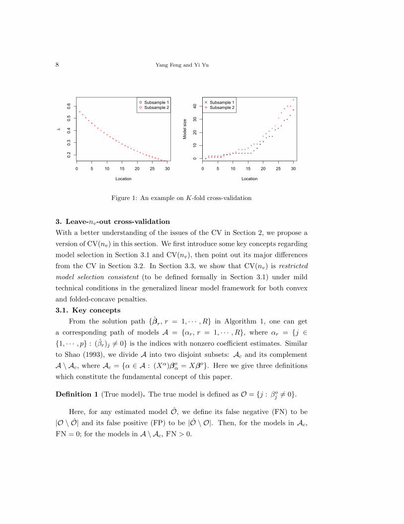
We now present the behavior of CV(nv) when nv varies through a simulation

study. In Figure 2, we present the average false positive (FP) and false negative

(FN) of CV(nv) with a wide range of nc in linear and logistic regression prob-

lems with n = 500 and p = 1000, with details of setting left in Example 1. From

Figure 2, it is clear that in all cases, the larger the order of nc is, the more FP

are involved, but the less FN. For linear regression, nc = dn1/2e has the best

performance, while nc = dn3/4e is the best for logistic regression. The differ-

ent behaviors for linear regression and logistic regression are due to the fact that

when the covariates and the coefficients are the same, the logistic regression needs

a larger sample size to fit the model well compare with linear regression. We pro-

vide some intuition as follows. Under the canonical link, the Fisher information

for generalized linear models can be written as 1/a(φ)X>WX, where φ is the dis-

persion parameter. For logistic regression, W = diag{π1(1−π1), · · · , πn(1−πn)},where πi = exp(x>i β)/(1 + exp(x>i β)) < 1 in non-degenerate cases; while for lin-

ear regression, W = In. This indicates that logistic regression always has less

information than linear regression, which leads to the fact that compared with

linear regression, we need a larger sample size for the logistic regression to have

the same level of estimation accuracy.

We conclude that in order to achieve the restricted model selection con-

sistency property, a small nc rate should be chosen as long as the size of the

construction sample is large enough to provide accurate estimates. Despite the

comparison above, the optimal nc rates may change for different settings. In any


case, CV(nv) with a wide range of nc values all lead to a better performance than

the 10-fold CV as well as AIC and BIC.

Different from Shao (1993, 1996), we are studying a high-dimensional variable

selection problem, which leads to fundamental technical differences. We allow

the number of candidate models to diverge, as stated in Condition 3 below, while

in Shao (1993, 1996) this quantity is a fixed constant.

3.3. Theory

Before presenting the theory, we introduce several conditions.

Condition 1. The set Ac is not empty.

Condition 1 is usually satisfied when the penalty parameter λ is small enough,

and it ensures that the problem we are trying to solve is not degenerate.

Condition 2 (Beta-min). For the true model O, let σ2 = var(y), we assume

β∗ = minj∈O

∣∣βoj ∣∣� σ

√log p

n.

Condition 2 is common in the high-dimensional sparse recovery literature,

which guarantees that the signal variables are detectable from the noise variables.

If p = O (exp (na)), 0 < a < 1, then β∗ = Θ(1) is sufficient to satisfy this

condition. In fact, β∗ can go to zero slowly as n and p diverge.

Condition 3 (Candidate set). Denote dmax = maxα∈Ac |α|, d∗ = max{dmax −d∗, d∗}. Assume ncd

∗ � n and

R = o (exp (n/(ncd∗))) . (3.2)

Condition 3 assures the candidate set is well behaved. The possible size of

the candidate set R can diverge at the rate in (3.2). We allow the number of

candidate models to diverge as long as ncd∗ � n. For instance, if d∗ is bounded

and nc = O(n1/2), then R = o(exp(n1/2)).

In the fixed p scenario, the candidate set can be all the possible 2p models.

When we allow both p and n to diverge, we are aware that the number of the can-

didate models increases too, although in practice this is usually a fixed number,

say, R = 100 in the default setting in the glmnet package in R. We can actually

control an increasing number of candidate models by exploiting concentration

inequalities. Condition 3 gives the limit of this quantity.


Figure 2: The average false positive (FP) and false negative (FN) of CV(nv) for different

nc values in Example 1.

(a) Linear regression, ρ = 0

0.35 0.40 0.45 0.50 0.55 0.60 0.65

01

23

45

log(nc) log(n)

aver

age

coun

t

FP FN

(b) Linear regression, ρ = 0.5

0.35 0.40 0.45 0.50 0.55 0.60 0.65

01

23

4

log(nc) log(n)

aver

age

coun

t

FP FN

(c) Logistic regression, ρ = 0

0.50 0.55 0.60 0.65 0.70 0.75 0.80

02

46

log(nc) log(n)

aver

age

coun

t

FP FN

(d) Logistic regression, ρ = 0.5

0.50 0.55 0.60 0.65 0.70 0.75 0.80

01

23

45

log(nc) log(n)

aver

age

coun

t

FP FN


Condition 4 (Generalized linear models properties). (i) Assume that b(·) has

continuous first, second and third order derivatives b(·), b(·) and...b (·); in addition,

b(·) > 0; (ii) there exists a function h(·) and ε0 > 0 such that for any α ∈ Acand ηα ∈ {ζα : ‖ζα − βα‖ ≤ ε0}, we have E(h(x)) < ∞, E(hα(xα)) < ∞,

‖b(x>αηα)‖2 ≤ hα(xα), and ‖...b (x>αηα)‖2 ≤ hα(xα) where hα(·) is the function

h(·) restricted to the subspace spanned by xα.

This is a mild condition for generalized linear models. For example, it is easy

to verify that the linear regression model satisfies Condition 4, since b(θ) = θ2/2,

in which case the function h(·) can be set as a constant function.

Condition 5 (Invertibility condition). There exist c∗ > 0 and q∗ = Θ(√n/ log p),

such that for all A ⊂ {1, · · · , p} with |A| = q∗ ≥ d∗ ≥ d0, and for any ηA ∈ {ζA :

‖ζA − βA‖ ≤ ε0}, where ε0 > 0 is fixed, and if v 6= 0 is a q∗-dimensional vector,

we have,

pr{c∗ ≤

∥∥(b(XAηA))1/2

XAv∥∥2/(n‖v‖2)}→ 1, n→∞.

This condition indicates that in any manifold of dimension less than or equal

to q∗, its corresponding restricted MLE is well-defined and unique. This is a

weaker version of the Sparse Riesz Condition (Zhang and Huang, 2008), in which

both upper and lower bounds are required. The Sparse Riesz Condition (or a

similar condition) was imposed in the existing literature on the tuning parameter

selection consistency using information criteria (Zhang et al., 2010). With the

invertibility condition, we can safely terminate the evaluation on the path when

the current model size exceeds q∗, without the risk of missing the optimal model.

Condition 6 (Design matrix). For all A ⊂ {1, · · · , p} with |A| = q∗, where q∗

is defined in Condition 5, and for any ηA ∈ {ζA : ‖ζA−βA‖ ≤ ε0}, where ε0 > 0

is a given constant, the following is satisfied,

maxs∈S

∥∥∥∥ 1

nv(XA

s )>b(XAs ηA)(XA

s )− 1

nc(XA

sc)>b(XA

scηA)XAsc

∥∥∥∥ = op(1),

where the norm here is the operator norm of matrices, sc = {1, · · · , n} \ s and Sis the collection of splits.

This condition bounds the difference between the Fisher information of the

validation set and the construction set. This is a reasonably mild condition with


the technical details of its corresponding version for linear models studied in

Section 4.4 of Shao (1993).

Theorem 1. For the penalized generalized linear models with separable sparse-

inducing penalties, assume Conditions 1-6 hold with nc/n→ 0, nc →∞, and the

number of the splits K satisfies

K−1n−2c n2 → 0.

Then, CV(nv) achieves restricted model selection consistency.

In Theorem 1, we do not explicitly specify the order of p as a condition,

however, the restriction on the dimensionality is implied by Conditions 2 and 3.

The ultra-high-dimensional setting where p = O(exp(na)), 0 < a < 1, is allowed.

Theorem 1 can be easily derived from Lemma 3 in the Appendix following the

fact that CV(nv) as described in Algorithm 2 nails a potentially high-dimensional

problem down to a low-dimensional one. With the selection consistency in hand,

the use of unpenalized solution in S4 of Algorithm 2 is applied to improve the

estimation and prediction performance.

4. Numerical experiments

In this section, we compare the proposed CV(nv) with several state-of-the-art

tuning parameter selection methods including the K-fold CV (K-fold), K-fold

CV with one standard error rule (1SE), AIC, BIC, and EBIC. We study both

the linear regression and logistic regression with different correlation structures

among covariates.

Before presenting the results of tuning parameter selection, we would like to

first examine the behavior of the collections of solutions generated via different

splits in a CV procedure.

4.1. Coherent Rate

Example 1. (i) Linear regression. For i = 1, · · · , n, let yi = x>i βo + εi, where

xii.i.d.∼ N (0p,Σ) with 0p the length-p vector with all 0 entries and Σj,k = ρ|j−k|,

εii.i.d.∼ N (0, 1), ρ = 0.5, (n, p) = (500, 10000) and βo ∈ Rp with the first 9

coordinates (0.8, 0, 0.7, 0, 0.6, 0, 0.5, 0, 0.4) and 0 elsewhere. (ii) Logistic regres-

sion. For i = 1, · · · , n, yi satisfies pr(yi = 1) = exp(x>i βo)/{1 + exp(x>i β

o)} =

1− pr(yi = 0), where βo ∈ Rp with the first 9 coordinates (1.6, 0, 1.4, 0, 1.2, 0,


1.0, 0, 0.8) and 0 elsewhere. The remaining part of the simulation setting is the

same as in (i).

Suppose the sequence of tuning parameters of the whole data set is λ =

(λ1, · · · , λR). Here, we take a variant of the 10-fold CV by repeatedly splitting

the whole data K = 100 times into 9/10 fraction as construction set and the re-

maining 1/10 fraction as the validation set. Denote the collection of the validation

sets as {sk, k = 1, · · · ,K} and the construction sets as {s(−k), k = 1, · · · ,K}.We also denote s0 = {1, · · · , n} to be the whole sample as a reference. Denote

by α(k)r the model of the r-th location in the collection of solutions constructed

by subset s(−k) using its corresponding tuning parameter sequence λ(−k), where

r = 1, · · · , R, k = 0, 1, · · · ,K. We define the coherent rate as a sequence rep-

resenting the degree of agreement of the models across different splits for each

tuning parameter location,

CR(r) =∣∣{k = 1, · · · ,K : α(k)

r = α(0)r }∣∣/K, r = 1, · · · , R.

In the ideal case where CR(r) = 1, for all r = 1, · · · , R, the CV method for

choosing the tuning parameter may serve as a good surrogate for selecting the

optimal model. However, this is rarely true in practice, especially after the noise

variables are activated in the estimators. Next, we demonstrate the behavior of

coherent rate.

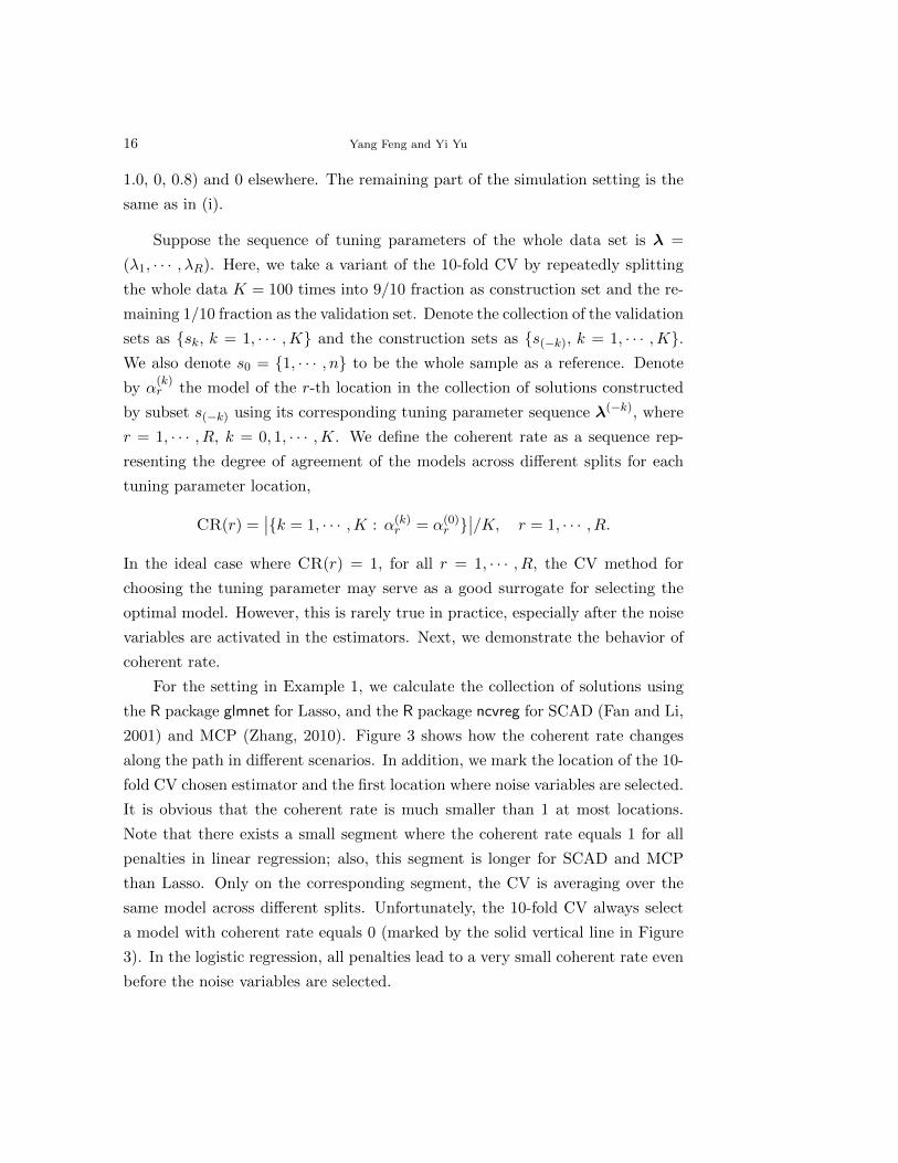
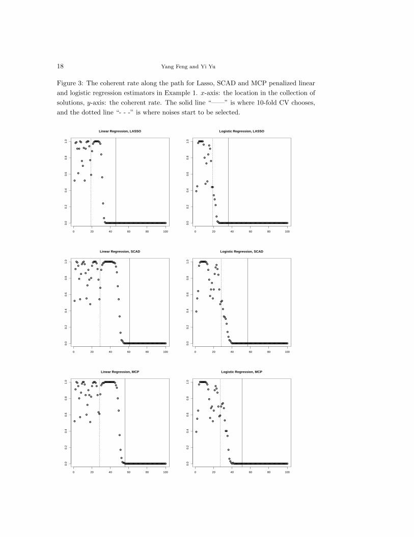
For the setting in Example 1, we calculate the collection of solutions using

the R package glmnet for Lasso, and the R package ncvreg for SCAD (Fan and Li,

2001) and MCP (Zhang, 2010). Figure 3 shows how the coherent rate changes

along the path in different scenarios. In addition, we mark the location of the 10-

fold CV chosen estimator and the first location where noise variables are selected.

It is obvious that the coherent rate is much smaller than 1 at most locations.

Note that there exists a small segment where the coherent rate equals 1 for all

penalties in linear regression; also, this segment is longer for SCAD and MCP

than Lasso. Only on the corresponding segment, the CV is averaging over the

same model across different splits. Unfortunately, the 10-fold CV always select

a model with coherent rate equals 0 (marked by the solid vertical line in Figure

3). In the logistic regression, all penalties lead to a very small coherent rate even

before the noise variables are selected.


From the path-generating procedure, estimators and tuning parameters can

be regarded as functions of each other, given the data, so the phenomenon we

noticed above is due to the data-driven property of tuning parameters selection.

When the data are changed from the whole sample to different subsample splits,

the tuning parameter sequence is usually different, and naturally leads to possibly

distinct models. If one wants to hold the models the same, very stringent con-

ditions need to be imposed on the design matrix; these are usually not satisfied

even for the simple simulation settings we have shown.

4.2. Linear regression

For linear regression, we use the same setting as Example 1 (i) with ρ = 0 and

ρ = 0.5, and repeat the simulation 100 times. Here the signal to noise ratio (SNR)

for the two settings are 1.9 and 4, respectively. For SCAD and MCP paths, we

use the default γ = 3 in the ncvreg package. In Table 1, for CV(nv), we set

nc = dn1/2e = 23 and nv = n − nc = 477. We compare our results with 10-fold

CV in glmnet and ncvreg. We also include the comparison with 10-fold CV with

1SE, where the λ is chosen as the maximum one with a loss function value less

than the minimum loss function value plus its standard error. In addition, we

report the performances of popular information criteria including AIC, BIC and

EBIC. To compare these methods, we report false negative (FN), false positive

(FP) and prediction error (PE) evaluated on an independent test data set of size

n.

In Table 1, for Lasso penalty, AIC and 10-fold CV have the largest mean FP

followed by BIC, 1SE and EBIC. CV(nv) performs the best in terms of FP, FN

as well as PE in both ρ = 0 and ρ = 0.5 cases.

SCAD and MCP lead to similar performances to Lasso based methods. Their

FP of 10-fold CV are not as large as those of Lasso, but CV(nv) still outperforms

10-fold CV and AIC in terms of both variable selection and prediction. It is

worth to point out that the difference is not as significant as that in the Lasso

case, possibly due to the asymptotic unbiasedness property of SCAD and MCP

(Zhang, 2010). It is similar that when using BIC and EBIC, SCAD and MCP

perform better than Lasso.

We also present the comparisons of the λ value derived from the universal

thresholding (Donoho and Johnstone, 1994) λuniv = σ√

2(log p)/n with σ being


Figure 3: The coherent rate along the path for Lasso, SCAD and MCP penalized linear

and logistic regression estimators in Example 1. x-axis: the location in the collection of

solutions, y-axis: the coherent rate. The solid line “——” is where 10-fold CV chooses,

and the dotted line “- - -” is where noises start to be selected.

●

●●

●

●

●

●●

●

●

●

●

●

●●●

●

●

●

●

●●●●●●●●

●

●

●

●

●

●●●●●●●●●●●●●●●●●●●●●●●●●●●●●●●●●●●●●●●●●●●●●●●●●●●●●●●●●●●●●●●●●●●

0 20 40 60 80 100

0.0

0.2

0.4

0.6

0.8

1.0

Linear Regression, LASSO

●

●

●●●●●●

●

●

●

●

●

●

●

●

●

●●

●

●

●

●

●●●●●●●●●●●●●●●●●●●●●●●●●●●●●●●●●●●●●●●●●●●●●●●●●●●●●●●●●●●●●●●●●●●●●●●●●●●●●

0 20 40 60 80 100

0.0

0.2

0.4

0.6

0.8

1.0

Logistic Regression, LASSO

●

●

●●

●

●

●

●

●●●

●

●

●

●

●

●

●

●

●

●●●●●

●

●

●

●

●

●●●●●●●●●●●●●●●

●

●

●

●

●

●

●●●●●●●●●●●●●●●●●●●●●●●●●●●●●●●●●●●●●●●●●●●●●●●●●

0 20 40 60 80 100

0.0

0.2

0.4

0.6

0.8

1.0

Linear Regression, SCAD

●

●

●

●

●●●●●●●●●

●

●

●

●

●

●

●

●

●

●

●

●

●

●

●●

●

●●●

●

●

●

●●●●●●●●●●●●●●●●●●●●●●●●●●●●●●●●●●●●●●●●●●●●●●●●●●●●●●●●●●●●●●●●

0 20 40 60 80 100

0.0

0.2

0.4

0.6

0.8

1.0

Logistic Regression, SCAD

●

●

●●

●

●

●

●

●●●

●

●

●

●

●

●

●

●

●

●●●●

●

●

●●

●

●●●●●●●●●●●●●●●●

●

●

●

●

●

●

●

●●●●●●●●●●●●●●●●●●●●●●●●●●●●●●●●●●●●●●●●●●●●●●●●

0 20 40 60 80 100

0.0

0.2

0.4

0.6

0.8

1.0

Linear Regression, MCP

●

●

●

●

●●●●●●●●●

●

●

●

●●

●

●

●

●

●

●

●

●●

●

●●

●

●

●●

●

●

●

●●●●●●●●●●●●●●●●●●●●●●●●●●●●●●●●●●●●●●●●●●●●●●●●●●●●●●●●●●●●●●●

0 20 40 60 80 100

0.0

0.2

0.4

0.6

0.8

1.0

Logistic Regression, MCP


Table 1: Comparisons for Example 1(i) with ρ = 0 and ρ = 0.5 cases. Results are

reported in the form of mean (standard error). For CV(nv), nc = dn1/2e and K = 50;

FP, false positive; FN, false negative; PE, prediction error.

Method ρ = 0 ρ = 0.5

Lasso FP FN PE FP FN PE

CV(nv) 0.01(0.01) 0.00(0.00) 1.01(0.01) 0.07(0.03) 0.04(0.02) 1.02(0.01)

10-fold 48.39(3.99) 0.00(0.00) 1.12(0.01) 30.72(3.04) 0.00(0.00) 1.09(0.01)

1SE 3.31(0.81) 0.00(0.00) 1.19(0.01) 1.51(0.37) 0.00(0.00) 1.16(0.01)

AIC 497.32(1.23) 0.00(0.00) 1.38(0.01) 471.54(1.36) 0.00(0.00) 1.37(0.01)

BIC 2.04(0.21) 0.00(0.00) 1.16(0.01) 1.75(0.15) 0.00(0.00) 1.12(0.01)

EBIC 0.58(0.08) 0.00(0.00) 1.18(0.01) 0.90(0.09) 0.00(0.00) 1.13(0.01)

SCAD FP FN PE FP FN PE

CV(nv) 0.02(0.01) 0.00(0.00) 1.01(0.01) 0.05(0.02) 0.00(0.00) 1.01(0.01)

10-fold 24.50(2.80) 0.00(0.00) 1.03(0.01) 21.74(2.37) 0.00(0.00) 1.03(0.01)

1SE 0.48(0.12) 0.00(0.00) 1.08(0.01) 0.21(0.05) 0.00(0.00) 1.08(0.01)

AIC 42.19(2.60) 0.00(0.00) 1.03(0.01) 27.02(1.89) 0.04(0.02) 1.07(0.02)

BIC 0.94(0.11) 0.00(0.00) 1.04(0.01) 0.77(0.11) 0.04(0.02) 1.08(0.02)

EBIC 0.30(0.05) 0.00(0.00) 1.05(0.01) 0.22(0.05) 0.04(0.02) 1.09(0.02)

MCP FP FN PE FP FN PE

CV(nv) 0.04(0.02) 0.00(0.00) 1.01(0.01) 0.06(0.02) 0.01(0.01) 1.01(0.01)

10-fold 4.87(0.66) 0.00(0.00) 1.02(0.01) 5.25(0.66) 0.00(0.00) 1.02(0.01)

1SE 0.01(0.01) 0.00(0.00) 1.07(0.01) 0.02(0.02) 0.01(0.01) 1.07(0.01)

AIC 87.14(0.45) 0.00(0.00) 1.18(0.01) 80.23(0.75) 0.00(0.00) 1.16(0.01)

BIC 1.20(0.90) 0.00(0.00) 1.02(0.01) 1.43(0.94) 0.00(0.00) 1.02(0.01)

EBIC 0.05(0.02) 0.00(0.00) 1.02(0.01) 0.06(0.02) 0.00(0.00) 1.02(0.01)

the error standard deviation and the λ values from different methods in Table 3

under the uncorrelated design (ρ = 0). The rationale of universal thresholding

is a theoretical upper bound of the maximum of all the errors; hence it can be

regarded as a theoretical lower bound of λ to remove all the noise variables. We

observe from the table that only CV(nv) gives a λ value larger than λuniv. On

the other hand, note that the lowest signal level of this example is 0.4, which can

serve as an upper bound of λ in order to retain all the important variables. This

analysis provides an explanation to the great performance of CV(nv).

We consider an additional simulation setting described in the following ex-


Table 2: Comparisons for Example 2 with ρ = 0 and ρ = 0.5 cases. Results are reported

in the form of mean (standard error). For CV(nv), nc = dn1/2e and K = 50; FP, false

positive; FN, false negative; PE, prediction error.


Lasso FP FN PE FP FN PE

CV(nv) 0.02(0.01) 0.01(0.01) 1.01(0.01) 0.03(0.02) 0.07(0.03) 1.02(0.01)

10-fold 73.56(5.13) 0.00(0.00) 1.17(0.01) 32.47(3.33) 0.00(0.00) 1.09(0.01)

1SE 7.44(0.83) 0.00(0.00) 1.23(0.01) 0.99(0.36) 0.00(0.00) 1.15(0.01)

AIC 484.59(1.39) 0.00(0.00) 1.41(0.01) 402.84(1.19) 0.00(0.00) 1.31(0.01)

BIC 3.41(0.26) 0.00(0.00) 1.24(0.01) 1.10(0.14) 0.00(0.00) 1.11(0.01)

EBIC 0.76(0.10) 0.00(0.00) 1.28(0.01) 0.26(0.05) 0.00(0.00) 1.12(0.01)

SCAD FP FN PE FP FN PE

CV(nv) 0.01(0.01) 0.01(0.01) 1.01(0.01) 0.04(0.02) 0.07(0.03) 1.02(0.01)

10-fold 19.80(2.35) 0.00(0.00) 1.02(0.01) 22.99(1.78) 0.00(0.00) 1.03(0.01)

1SE 0.20(0.06) 0.00(0.00) 1.08(0.01) 1.13(0.23) 0.02(0.01) 1.07(0.01)

AIC 214.58(1.31) 0.00(0.00) 1.49(0.02) 34.73(2.48) 0.00(0.00) 1.03(0.01)

BIC 0.82(0.11) 0.00(0.00) 1.04(0.01) 1.05(0.16) 0.01(0.01) 1.05(0.01)

EBIC 0.19(0.04) 0.00(0.00) 1.04(0.01) 0.30(0.06) 0.02(0.01) 1.06(0.01)

MCP FP FN PE FP FN PE

CV(nv) 0.01(0.01) 0.01(0.01) 1.01(0.01) 0.04(0.02) 0.07(0.03) 1.02(0.01)

10-fold 6.46(1.01) 0.00(0.00) 1.02(0.01) 7.16(0.76) 0.00(0.00) 1.03(0.01)

1SE 0.01(0.01) 0.00(0.00) 1.07(0.01) 0.05(0.03) 0.06(0.02) 1.07(0.01)

AIC 102.30(0.48) 0.00(0.00) 1.81(0.02) 46.67(1.04) 0.00(0.00) 1.06(0.01)

BIC 100.72(1.13) 0.00(0.00) 1.80(0.02) 0.66(0.19) 0.01(0.01) 1.03(0.01)

EBIC 0.06(0.03) 0.00(0.00) 1.02(0.01) 0.07(0.03) 0.02(0.01) 1.03(0.01)

ample.

Example 2. Linear regression. For i = 1, · · · , n, let yi = x>i βo + εi, where

xii.i.d.∼ N (0p,Σ) with 0p the length-p vector with all 0 entries and Σj,k = ρ|j−k|,

εii.i.d.∼ N (0, 1), ρ = 0 or 0.5, (n, p) = (500, 10000) and βo ∈ Rp with the first 7

coordinates (1, 0.9, 0.8, 0.7, 0.6, 0.5, 0.4) and 0 elsewhere.

Note that this is a more challenging scenario compared with Example 1(i)

since there are more signal variables and the correlation among signal variables

is stronger when ρ = 0.5. The corresponding results for Example 2 are available


Table 3: Comparison of λ values derived from various methods for Example 2 (i) with

ρ = 0. Results are presented in the form of mean (standard error).

Universal CV(nv) 10-fold 1SE AIC BIC EBIC

0.19 0.20(0.02) 0.12(0.02) 0.18(0.02) 0.01(0.00) 0.17(0.01) 0.18(0.01)

in Table 2. For ρ = 0 with Lasso penalty, CV(nv) performs significantly better

than all the competing methods in terms of both FP and PE. We observe similar

conclusions for other settings.

4.3. Logistic regression

For logistic regression, we use the setting in Example 1 (ii) with ρ = 0 and

ρ = 0.5, and repeat the simulation 100 times. In Table 4, for CV(nv), we set

nc = dn3/4e = 106 following the results in Section 3.2. Different from the linear

case, instead of reporting PE, we report classification error (CE), which is defined

as the average classification error evaluated at an independent test data set of

size n. The remaining settings and packages used are the same as in the linear

regression case.

In Table 4, CV(nv) significantly outperforms 10-fold CV and AIC in terms

of FP. The difference is more significant than that in the linear regression case,

when SCAD or MCP is used. For Lasso penalized logistic regression, 1SE has a

significant number of FP, compared with the linear regression case. EBIC tends

to work much better than AIC and BIC, with a similar performance as CV(nv)

when SCAD and MCP are applied. When evaluated by the CE, CV(nv) still

performs the best in most scenarios.

5. Data Analysis

We now illustrate two applications of the proposed method via eye disease

gene expression data (Scheetz et al., 2006) and leukemia data set (Golub et al.,

1999).

In the eye disease gene expression data set, for harvesting of tissue from the

eyes and subsequent microarray analysis, 120 12-week-old male rats were selected.

The microarrays used to analyze the RNA from the eyes of these animals contain

more than 31,042 different probe sets (Affymetric GeneChip Rat Genome 230

2.0 Array). The intensity values were normalized using the robust multichip


Table 4: Comparison in Logistic regression with ρ = 0 and ρ = 0.5 cases. Results are

reported in the form of mean (standard error). For CV(nv), nc = dn3/4e and K = 50;

FN, false negative; FP, false positive; CE, classification error.


Lasso FP FN CE(%) FP FN CE(%)

CV(nv) 1.63(0.14) 0.01(0.01) 19.34(0.20) 0.92(0.10) 0.10(0.03) 16.06(0.20)

10-fold 95.86(4.60) 0.00(0.00) 20.81(0.23) 87.76(4.28) 0.01(0.01) 17.22(0.20)

1SE 21.48(2.05) 0.00(0.00) 19.44(0.20) 15.60(1.67) 0.03(0.02) 16.19(0.18)

AIC 21.63(1.34) 0.00(0.00) 19.50(0.20) 20.01(1.56) 0.02(0.01) 16.28(0.19)

BIC 1.88(0.14) 0.08(0.03) 19.49(0.19) 1.75(0.16) 0.05(0.02) 16.14(0.18)

EBIC 0.46(0.07) 0.16(0.04) 19.72(0.20) 0.60(0.08) 0.11(0.03) 16.25(0.18)

SCAD FP FN CE(%) FP FN CE(%)

CV(nv) 1.84(0.13) 0.02(0.01) 19.48(0.22) 1.17(0.12) 0.08(0.03) 16.21(0.19)

10-fold 55.05(2.06) 0.00(0.00) 19.22(0.20) 52.40(1.93) 0.02(0.01) 16.72(0.19)

1SE 10.88(0.76) 0.00(0.00) 19.34(0.19) 8.29(0.70) 0.03(0.02) 16.40(0.18)

AIC 31.24(1.25) 0.00(0.00) 19.20(0.20) 23.84(1.34) 0.06(0.02) 16.48(0.19)

BIC 3.23(0.26) 0.03(0.02) 19.61(0.19) 2.17(0.20) 0.08(0.03) 16.41(0.19)

EBIC 0.92(0.10) 0.11(0.03) 19.90(0.19) 0.77(0.08) 0.10(0.03) 16.54(0.19)

MCP FP FN CE(%) FP FN CE(%)

CV(nv) 2.08(0.12) 0.02(0.01) 19.76(0.20) 1.36(0.10) 0.06(0.02) 16.60(0.19)

10-fold 13.10(0.79) 0.00(0.00) 18.84(0.21) 13.31(0.87) 0.03(0.02) 16.23(0.19)

1SE 0.91(0.14) 0.06(0.02) 19.13(0.19) 1.09(0.22) 0.10(0.03) 16.25(0.19)

AIC 19.38(1.08) 0.00(0.00) 18.92(0.20) 33.39(1.02) 0.03(0.02) 16.86(0.20)

BIC 2.51(0.23) 0.03(0.02) 18.88(0.20) 2.16(0.27) 0.08(0.03) 16.06(0.18)

EBIC 0.49(0.07) 0.07(0.03) 18.97(0.19) 0.32(0.06) 0.13(0.03) 16.16(0.18)

averaging method (Irizarry et al., 2003) to obtain summary expression values for

each probe set. Gene expression levels were analyzed on a logarithmic scale.

Following Huang et al. (2010) and Fan et al. (2011), we are interested in

finding the genes that are related to the TRIM32 gene, which was recently found

to cause Bardet–Biedl syndrome (Chiang et al., 2006) and is a genetically hetero-

geneous disease of multiple organ systems, including the retina. Although more

than 30,000 probe sets are represented on the Rat Genome 230 2.0 Array, many

of these are not expressed in the eye tissue. We focus only on the 18,975 probes

that are expressed in the eye tissue.


Table 5: Model size and prediction error for the Eye Disease Gene Expression data sets.

Results are reported in the form of mean (standard error).

Lasso SCAD MCP

Method Size PE Size PE Size PE

CV(nv) 2.46(0.08) 0.01(0.00) 2.23(0.07) 0.01(0.00) 2.36(0.07) 0.01(0.00)

10-fold 61.18(1.68) 0.01(0.00) 33.54(0.59) 0.01(0.00) 11.12(0.30) 0.01(0.00)

1SE 31.03(1.16) 0.01(0.00) 24.84(0.71) 0.01(0.00) 5.39(0.31) 0.01(0.00)

AIC 103.02(0.48) 0.01(0.00) 0.37(0.05) 0.02(0.00) 5.38(0.25) 0.01(0.00)

BIC 99.99(0.71) 0.01(0.00) 0.17(0.04) 0.02(0.00) 4.65(0.25) 0.01(0.00)

EBIC 1.03(0.24) 0.02(0.00) 0.02(0.01) 0.02(0.00) 1.90(0.13) 0.01(0.00)

The leukemia data set we studied was previously analyzed in Golub et al.

(1999). There are p = 7, 129 genes and n = 72 samples coming from two classes:

47 in class ALL (acute lymphocytic leukemia) and 25 in class AML (acute myel-

ogenous leukemia).

We model these two problems using linear and logistic regression, respec-

tively. In the eye gene expression data set, we randomly draw without replace-

ment 100 out of 120 observations from the sample, using them as training data,

and use the remaining sub-sample of size 20 as the test data. In the leukemia

data set, we randomly draw without replacement 60 out of 72 observations from

the sample as the training data with the remaining observations as the test data.

We repeat this procedure 100 times with the results reported in Tables 5

and 6 in the form of mean (standard error). For each split, we use glmnet and

ncvreg to compute the Lasso and SCAD / MCP collections of solutions, respec-

tively; we then compare our proposed CV(nv) with the 10-fold CV, which is the

default tuning parameter selection method in glmnet and ncvreg. In addition, we

investigate the performance of 1SE, AIC, BIC and EBIC.

For the eye disease gene expression data sets, Table 5 shows that CV(nv)

performs well compared with 10-fold CV as well as all the considered information

type criteria. In terms of model size, EBIC leads to the smallest model on average

when using the Lasso penalty. It, however, probably misses some important

predictors as the prediction error is larger than those of the other methods.


Table 6: Model size and test classification error for the Leukemia data sets. Results are

reported in the form of mean (standard error).

LASSO SCAD MCP

Method Size CE(%) Size CE(%) Size CE(%)

CV(nv) 8.93(0.58) 8.07(0.75) 10.14(0.57) 7.80(0.79) 5.62(0.14) 8.33(0.76)

10-fold 21.52(0.41) 5.85(0.74) 17.04(0.31) 7.45(0.75) 5.07(0.14) 9.84(0.94)

1SE 12.51(0.46) 8.87(0.93) 11.70(0.43) 9.84(0.92) 2.85(0.16) 14.54(1.25)

AIC 16.17(0.39) 6.65(0.76) 1.00(0.05) 30.59(1.37) 4.14(0.17) 10.02(0.98)

BIC 4.32(0.30) 17.20(1.14) 0.91(0.06) 30.59(1.37) 3.56(0.15) 10.37(1.01)

EBIC 0.48(0.06) 31.29(1.33) 0.37(0.05) 31.56(1.32) 1.46(0.08) 14.72(1.03)

Among the models that give the best prediction error, CV(nv) always selects the

sparsest model. Similar behaviors can be found in SCAD and MCP, though the

differences in performances are not as pronounced.

For the leukemia data set, we can see from Table 6 that both BIC and

EBIC select very small models with a large test classification error for all three

penalties. CV(nv) tends to provide a reasonably good balance for the complexity

of the model and the test classification error. Although 10-fold CV has a smaller

test classification error for Lasso and SCAD, it selects many more variables on

average.

6. Discussion

In this paper we study CV methods applied to the tuning parameter selection

problem in high-dimensional penalized generalized linear models. For the K-fold

CV, we show the issue of the mis-alignment for different splits is one possible

reason of over-selection. We advocate the use of CV(nv) with a proper choice of

nv for the path algorithms, which has been shown to be restricted model selection

consistent in high-dimensional settings.

One possible future direction is to study the theoretical implication of low

coherent rate of CV, as demonstrated in the numerical results, on the model selec-

tion performance. The proposed algorithm is a general framework, which could

be extended to the case of using other methods (e.g., forward regression) to gen-

erate the collection of solutions. It is also interesting to extend the methodology

BIBLIOGRAPHY 25

and the associated theory to other models including additive models, Cox propor-

tional hazards models, among others. In addition, we are interested in selecting

the concavity parameter γ in folded-concave penalties via cross-validation.

An implementation of the CV(nv) method for high-dimensional variable se-

lection is available at https://github.com/statcodes/rccv.

Supplementary Materials

The online supplementary materials include all the technical details and

additional simulation results.

Acknowledgements

The authors would like to thank the co-Editor Professor Hsin-Cheng Huang,

the AE and three referees for their insightful comments, which have greatly im-

proved the scope and quality of the paper. This research was partially supported

by NSF CAREER grant DMS-1554804.

Bibliography

Breheny, P. and Huang, J. (2011). Coordinate descent algorithms for non-

convex penalized regression, with applications to biological feature selection.

The Annals of Applied Statistics, 5 232–253.

Buhlmann, P. and van de Geer, S. (2011). Statistics for High-Dimensional

Data. Springer-Verlag New York Inc.

Chen, J. and Chen, Z. (2008). Extended bayesian information criteria for

model selection with large model spaces. Biometrika, 95 759–71.

Chen, S. and Donoho, D. (1994). Basis pursuit. In 1994 Conference Record of

the Twenty-Eighth Asilomar Conference on Signals, Systems and Computers,

vol. 1. IEEE, 41–4.

Chiang, A. P., Beck, J. S., Yen, H.-J., Tayeh, M. K., Scheetz, T. E.,

Swiderski, R. E., Nishimura, D. Y., Braun, T. A., Kim, K.-Y. A.,

Huang, J., Elbedour, K., Carmi, R., Slusarski, D. C., Casavant,

https://github.com/statcodes/rccv


T. L., Stone, E. M. and Sheffield, V. C. (2006). Homozygosity map-

ping with snp arrays identifies trim32, an e3 ubiquitin ligase, as a bardet–biedl

syndrome gene (bbs11). Proc. Natl. Acad. Sci. U.S.A., 103 6287–92.

Donoho, D. L. and Johnstone, I. M. (1994). Ideal spatial adaptation by

wavelet shrinkage. Biometrika, 81 425–455.

Efron, B. (1983). Estimating the error rate of a prediction rule: Improvement

on cross-validation. Biometrika, 78 316–31.

Efron, B. (1986). How biased is the apparent error rate of a prediction rule?

J. Am. Statist. Assoc., 81 461–70.

Efron, B., Hastie, T., Johnstone, I., Tibshirani, R. et al. (2004). Least

angle regression. The Annals of statistics, 32 407–499.

Fan, J., Feng, Y. and Song, R. (2011). Nonparametric independence screening

in sparse ultra-high-dimensional additive models. J. Am. Statist. Assoc., 106

544–57.

Fan, J. and Li, R. (2001). Variable selection via nonconcave penalized likelihood

and its oracle properties. J. Am. Statist. Assoc., 96 1348–60.

Fan, J. and Lv, J. (2010). A selective overview of variable selection in high

dimensional feature space. Statistica Sinica, 20 101–148.

Fan, Y. and Tang, C. Y. (2013). Tuning parameter selection in high-

dimensional penalized likelihood. Journal of the Royal Statistical Society, Ser.

B., 75 531–552.

Friedman, J. et al. (2010). Regularization paths for generalized linear models

via coordinate descent. J. Statist. Softw., 33 1–22.

Golub, T. R., Slonim, D. K., Tamayo, P., Huard, C., Gaasenbeek, M.,

Mesirov, J. P., Coller, H., Loh, M. L., Downing, J. R., Caligiuri,

M. A., Bloomfield, C. D. and Lander, E. S. (1999). Molecular clas-

sification of cancer: class discovery and class prediction by gene expression

monitoring. Science, 286 531–37.

BIBLIOGRAPHY 27

Huang, J., Horowitz, J. L. and Wei, F. (2010). Variable selection in non-

parametric additive models. Ann. Statist., 38 2282–313.

Irizarry, R. A., Hobbs, B., Collin, F., Beazer-Barclay, Y. D., An-

tonellis, K. J., Scherf, U. and Speed, T. P. (2003). Exploration, nor-

malization, and summaries of high density oligonucleotide array probe level

data. Biostatistics, 4 249–64.

Luo, S. and Chen, Z. (2014). Sequential lasso cum ebic for feature selection

with ultra-high dimensional feature space. Journal of the American Statistical

Association, 109 1229–1240.

Meinshausen, N. (2007). Relaxed lasso. Comput. Stat. Data Anal., 52 374–93.

Park, M. Y. and Hastie, T. (2007). An l1 regularization-path algorithm for

generalized linear models. J. R. Statist. Soc. B, 69 659–677.

Scheetz, T. E., Kim, K.-Y. A., Swiderski, R. E., Philp, A. R., Braun,

T. A., Knudtson, K. L., Dorrance, A. M., DiBona, G. F., Huang, J.,

Casavant, T. L., Sheffield, V. C. and Stone, E. M. (2006). Regulation

of gene expression in the mammalian eye and its relevance to eye disease. Proc.

Natl. Acad. Sci. U.S.A., 103 14429–34.

Shao, J. (1993). Linear model selection by cross-validation. J. Am. Statist.

Assoc., 88 486–94.

Shao, J. (1996). Bootstrap model selection. J. Am. Statist. Assoc., 91 655–65.

Stadler, N., Buhlmann, P. and Van De Geer, S. (2010). l1-penalization

for mixture regression models. Test, 19 209–256.

Stone, M. (1977). An asymptotic equivalence of choice of model by cross-

validation and akaike’s criterion. J. R. Statist. Soc. B, 39 44–7.

Sun, T. and Zhang, C.-H. (2012). Scaled sparse linear regression. Biometrika,

99 879–898.

Tibshirani, R. (1996). Regression shrinkage and selection via the lasso. J. R.

Statist. Soc. B, 9 267–88.


Wang, H., Li, B. and Leng, C. (2009). Shrinkage tuning parameter selection

with a diverging number of parameters. Journal of the Royal Statistical Society:

Series B (Statistical Methodology), 71 671–683.

Wang, H., Li, R. and Tsai, C.-L. (2007). Tuning parameter selectors for the

smoothly clipped absolute deviation method. Biometrika, 94 553–68.

Yu, Y. and Feng, Y. (2014a). Apple: Approximate path for penalized likelihood

estimators. Statistics and Computing, 24 803–819.

Yu, Y. and Feng, Y. (2014b). Modified cross-validation for penalized high-

dimensional linear regression models. Journal of Computational and Graphical

Statistics, 23 1009–1027.

Zhang, C.-H. (2010). Nearly unbiased variable selection under minimax concave

penalty. Ann. Statist., 38 894–942.

Zhang, C.-H. and Huang, J. (2008). The sparsity and bias of the lasso selection

in high-dimensional linear regression. Ann. Statist., 36 1567–94.

Zhang, Y., Li, R. and Tsai, C.-L. (2010). Regularization parameter selections

via generalized information criterion. J. Am. Statist. Assoc., 105 312–23.

Department of Statistics, Columbia University

E-mail: [email protected]

School of Mathematics, University of Bristol

E-mail: [email protected]

BIBLIOGRAPHY 29

Supplementary materials for “The restricted consistency

property of leave-nv-out cross-validation for

high-dimensional variable selection”

Yang Feng and Yi Yu

Columbia University and University of Bristol

The supplementary material includes all the technical details and additional simulation

results.

A.1 Additional lemmas and proofs

The following Lemma is adapted from ?). It helps us to develop the asymptotic theory

where N , the size of the candidate models, is allowed to diverge with the sample size.

Lemma 1 (Gaussian concentration). Let γ be the standard Gaussian probability measure on

Rn (that is, the distribution of a N (0, In) random vector), and let F : Rn → R be Lipschitz in

each variable separately relative to the Euclidean metric, with Lipschitz constant c. Then for

every t > 0,

γ{|F − Eγ(F )| ≥ t} ≤ 2 exp

(− t2

c2π2

).

Lemma 2. With p < n, let β be the MLEs of a generalized linear model. Assume the penalty

function p(·) is separable, and assume Conditions 1 - 6 hold. Furthermore, assume nc → ∞and nc/n→ 0 as n→∞, and the size of the splits K satisfies

K−1n−2c n2 → 0.

Then, CV(nv) with K times subsampling is restricted model selection consistent.

Proof of Lemma 2. Due to the properties of generalized linear models with canonical parameter,

we have

E(yi | xi) = b(x>i β), σ2i = a(φ)b(x>i β), i = 1, · · · , n,

and define σ2 = (1/n)∑ni=1 σ

2i . The target is to select the model that minimizes the loss

Γα =1

Knv

∑s∈S

{−y>s (Xα

s βsc,α) + 1>b(Xαs βsc,α)

}, (3.3)

where S represents the collection of validation sets in different splits and 1 is an all-one vector.

Denote ES and varS as the expectation and variance with respect to the random selection

of S. By using the equality

ES

(1

r

∑s∈S

as

)=

(n

nv

)−1 ∑s∈ all s

E(as),


rewriting (3.3), and denoting `s(β) = y>s (Xsβ) − 1>b(Xsβ) and `n(βα) = y>(Xαβα) −1>b(Xαβα), we have

ES(Γα) =ES

(− 1

Knv

∑s∈S

`s(βo)

)+ ES

(1

Knv

∑s∈S

{`s(β

o)−(y>s (Xα

s βα)− 1>b(Xαs βα)

)})+ES

(1

Knv

∑s∈S

{(y>s (Xα

s βα)− 1>b(Xαs βα)

)−(y>s (Xα

s βsc,α)− 1>b(Xαs βsc,α)

)})=E

(− 1

n`n(βo) +

1

n

(`n(βo)− `n(βα)

)+

(n

nv

)−1 ∑s∈ all s

1

nv

{y>s (Xα

s βα −Xαs βsc,α)− 1>

(b(Xα

s βα)− b(Xαs βsc,α)

)})

=− 1

nE(`n(βo)) + E(Aα1) +

(n

nv

)−1 ∑s∈ all s

E(Aα2,s).

For different α, E(`n(βo)) stays the same, so we only need to focus on Aα1 and Aα2,s.

From Wilks’ theorem, it is known that, if α ∈ A \ Ac, as n → ∞, we have Aα1D→

(1/2)χ2(kα), where kα = d0 − dα0, dα0 = |{j : βj ∈ α ∩ α0}|, i.e., kα is the number of false

negatives. This means E(Aα1) = kα; otherwise, E(Aα1) = O(1/n).

For any s,

1>(b(Xα

s βα)− b(Xαs βsc,α)

)=(b(Xα

s βα))>Xαs (βα − βsc,α)

− 1

2(βα − βsc,α)>(Xα

s )>b(Xαs βα)Xs,α(βα − βsc,α) + o(1).

Define usc(γ) = (1/nc)(Xαsc)>(ysc − b(Xα

scγ)), then βsc,α is the solution to usc(γ) = 0. By

Taylor expansion, we get

βα − βsc,α =(usc(βα)

)−1usc(βα)(1 + o(1)),

where usc(βα) = −(1/nc)(Xαsc)>b(Xα

sc βα)Xαsc .

Define Ds,α = b1/2(Xαs βα)Xα

sc , then

Aα2,s =1

nv

(ys − b(X

αs βα)

)>Xαs (βα − βsc,α)

+1

2nv(βα − βsc,α)>(Xα

s )>b(Xαs βα)Xα

s (βα − βsc,α) + o(1/nv)

=1

nv

(ys − b(X

αs βα)

)>Xαs

(usc(βα)

)−1usc(βα) + o(1/nv)

+1

2nv

(ysc − b(X

αsc βα)

)>(b(Xα

s βα)−1/2)Ds,α(D>s,αDs,α)−1

×((Xα

s )>b(Xαs βα)Xα

s

)((Xα

sc)>b(Xα

s βα)Xαsc)−1

×D>s,α(b(Xα

s βα)−1/2)(ysc − b(Xαsc βα)

)(1 + o(1))

= Bα + Cα.

BIBLIOGRAPHY 31

By plugging in the expansion form of usc(·) and usc(·),

Bα = − 1

nv

(ys − b(X

αs βα)

)>Xαs

((Xα

sc)>b(Xα

sc βα)Xαsc)−1

(Xαsc)>(ysc − b(Xα

sc βα))(1 + o(1)).

From Conditions 5 and 6, straight calculations lead to

E(Bα) = 0, var(Bα) = dαa(φ)(ncnv)−1/2(1 + o(1)).

For Cα we have,

Cα =1

2nc

(ysc − b(X

αsc βα)

)>(b(Xα

s βα)−1/2)Ds,α(D>s,αDs,α)−1D>s,α

×(b(Xα

s βα)−1/2)(ysc − b(Xαsc βα)

)(1 + o(1)).

Thus, after taking expectation we have,

E(Aα2,s) = dαa(φ)/nc + o(1/nc).

If α ∈ A \ Ac,

Γα∗ − Γα =1

n

(`n(βα∗)− `n(βα)

)+O(1/nc).

From Lemma 1 and Condition 3, by exploiting Gaussian concentration, ∀ε > 0, we have

R · pr

{nc

∣∣∣∣ maxα∈A\Ac

∣∣∣ 1n

(`n(βα∗)− `n(βα)

)∣∣∣− E( maxα∈A\Ac

∣∣∣ 1n

(`n(βα∗)− `n(βα)

)∣∣∣)∣∣∣∣ > ε

}→ 0.

The parallel result for α ∈ Ac but α 6= α∗ holds similarly. Therefore, as n→∞, pr{α ∈ α∗} →1.

A.2 Additional numerical results

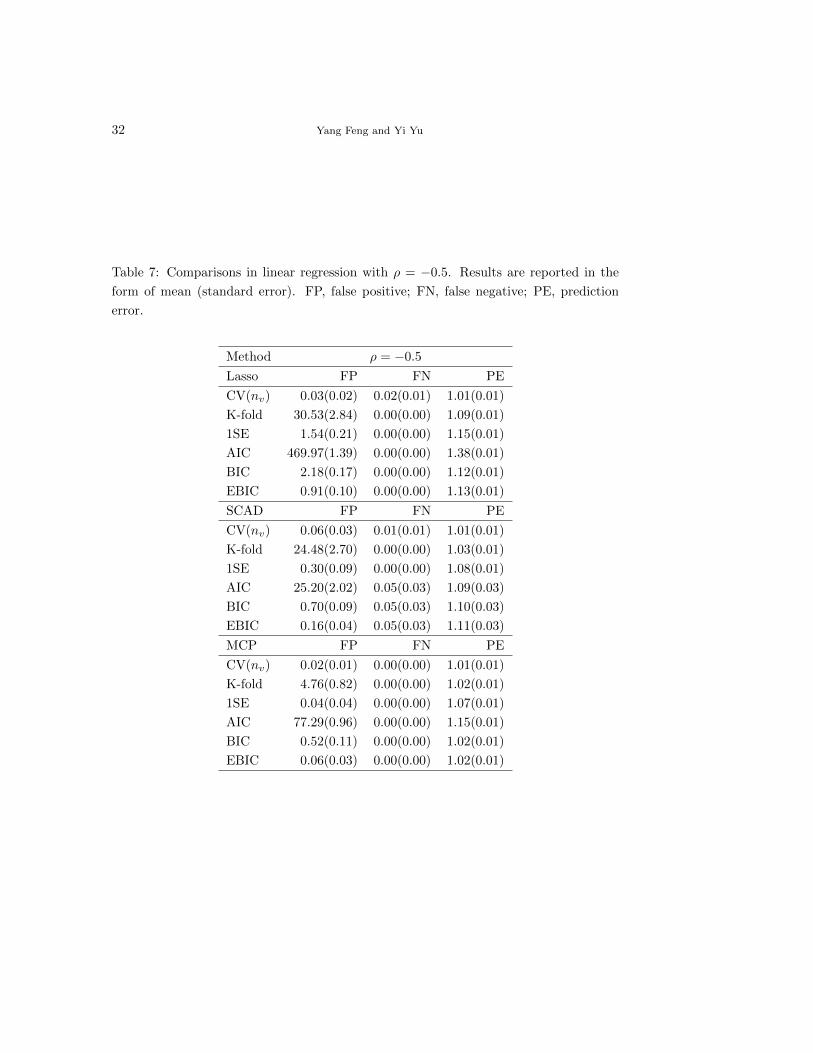
We conducted an additional simulation for the setting in Example 1(i) when ρ = −0.5

with the results summarized in Table 7. In this case, CV(nv) works very well compared with

other methods and we skip the detailed discussion since the message is very similar to the cases

of ρ = 0 and ρ = 0.5.


Table 7: Comparisons in linear regression with ρ = −0.5. Results are reported in the

form of mean (standard error). FP, false positive; FN, false negative; PE, prediction

error.

Method ρ = −0.5

Lasso FP FN PE

CV(nv) 0.03(0.02) 0.02(0.01) 1.01(0.01)

K-fold 30.53(2.84) 0.00(0.00) 1.09(0.01)

1SE 1.54(0.21) 0.00(0.00) 1.15(0.01)

AIC 469.97(1.39) 0.00(0.00) 1.38(0.01)

BIC 2.18(0.17) 0.00(0.00) 1.12(0.01)

EBIC 0.91(0.10) 0.00(0.00) 1.13(0.01)

SCAD FP FN PE

CV(nv) 0.06(0.03) 0.01(0.01) 1.01(0.01)

K-fold 24.48(2.70) 0.00(0.00) 1.03(0.01)

1SE 0.30(0.09) 0.00(0.00) 1.08(0.01)

AIC 25.20(2.02) 0.05(0.03) 1.09(0.03)

BIC 0.70(0.09) 0.05(0.03) 1.10(0.03)

EBIC 0.16(0.04) 0.05(0.03) 1.11(0.03)

MCP FP FN PE

CV(nv) 0.02(0.01) 0.00(0.00) 1.01(0.01)

K-fold 4.76(0.82) 0.00(0.00) 1.02(0.01)

1SE 0.04(0.04) 0.00(0.00) 1.07(0.01)

AIC 77.29(0.96) 0.00(0.00) 1.15(0.01)

BIC 0.52(0.11) 0.00(0.00) 1.02(0.01)

EBIC 0.06(0.03) 0.00(0.00) 1.02(0.01)

statistica sinica - arxiv · statistica sinica 1 the restricted consistency property of leave-n...

Documents