statistica sinica (2013): preprintstatistica sinica (2013): preprint 1 longitudinal functional...

Statistica Sinica (2013): Preprint 1

Longitudinal Functional Models with Structured Penalties

Madan G. Kundu1, Jaroslaw Harezlak1 and Timothy W. Randolph2

1Department of Biostatistics

Indiana University Fairbanks School of Public Health

Indianapolis, USA

2Biostatistics and Biomathematics Program

Fred Hutchinson Cancer Research Center

Seattle, USA

Abstract: This paper addresses estimation in a longitudinal regression model for as-

sociation between a scalar outcome and a set of longitudinally-collected functional

covariates or predictor curves. The framework consists of estimating a time-varying

coefficient function that is modeled as a linear combination of time-invariant func-

tions but having time-varying coefficients. The estimation procedure exploits the

equivalence between penalized least squares estimation and a linear mixed model

representation. The process is empirically evaluated with several simulations and

it is applied to analyze the neurocognitive impairment of HIV patients and its

association with longitudinally-collected magnetic resonance spectroscopy curves.

Key words and phrases: Functional data analysis, longitudinal data, mixed model,

structured penalty, generalized singular value decomposition

1 Introduction

Technological advancements and increased availability of storage of large datasets

have allowed for the collection of functional data as part of time-course or lon-

gitudinal studies. In the cross-sectional setting, there have been many proposed

methods for estimating a regression function in a so-called functional linear model

(fLM). This function is a functional (continuous) analogue of a vector of (dis-

crete) regression coefficients; it connects the scalar response, y to a functional

covariate, w ≡ w(s). Although these models have recently been well studied, ex-

tensions to longitudinally-collected functions have not received much attention.

arX

iv:1

211.

4763

v2 [

stat

.AP]

3 J

un 2

014

2 MADAN KUNDU, JAROSLAW HAREZLAK AND TIMOTHY RANDOLPH

Only recently longitudinal penalized functional regression (LPFR) and longitu-

dinal functional principal component regression (LFPCR) approaches have been

proposed to extend the cross-sectional fLM to a longitudinal setting by incor-

porating subject-specific random intercepts (Goldsmith et al., 2012; Gertheiss et

al., 2013). A basic assumption in both LPFR and LFPCR is that the regres-

sion function remains constant over time. Consequently, these methods are not

suited for situations in which the association between a functional predictor and

scalar response may evolve over time. Here we propose a technique that extends

the analysis of functional linear models by relating a scalar outcome to a func-

tional predictor—both observed longitudinally—and estimates a time-dependent

regression function.

The method fits into a generalized ridge regression framework by imposing a

scientifically-informed quadratic penalty term into the estimation process. The

extension of this framework to the longitudinal setting has two major advantages:

1) the regression function is allowed to vary over time; and 2) external or a priori

information about the structure of the regression function can be incorporated

directly into the estimation process. We formulate the estimation procedure

within a mixed-model framework making the method computationally efficient

and easy to implement.

Ramsay and Dalzell (1991) introduced the term functional data analysis

(FDA) in the statistical literature. The cross-sectional fLM with scalar response

can be stated as follows (see e.g., Yao and Muller, 2010)

E(y|W ) = µy +

∫ΩW (s)γ(s)ds

where µy is the mean of y, Ω denotes the domain of the predictor functions W (s),

s ∈ Ω, and γ(s) is a square integrable function that models the linear relationship

between the functional predictor and scalar response. We will assume that W (·)denotes a mean-centered function (E[W (s)] = 0 for almost all s ∈ Ω).

As there is no unique γ(·) that solves this equation some form of regulariza-

tion, or constraint, is required. For example, a common approach is to impose

smoothness on γ(·). One approach to this is to expand both the regression func-

tion γ(·) and predictor functions W (·) in terms of B-splines and then obtain the

regularized estimate of γ(·) (Ramsay and Silverman, 1997). Another approach

LONGITUDINAL FUNCTIONAL MODELS WITH STRUCTURED PENALTIES 3

is to express the regression function γ(·) in terms of the empirical orthonormal

basis obtained by the eigenfunctions of the covariance of W (·) (i.e., a Karhunen-

Loeve (K-L) expansion (see e.g., Muller , 2005)). A third approach, known

as penalized functional regression (PFR) (Goldsmith et al., 2011), combines the

above two methods. In PFR, a spline basis is used to represent γ(·) and a subset

of empirical eigenfunctions is used to represent each W (·). Another approach

is to use a wavelet basis, instead of splines or eigenfunctions, to represent the

predictor functions (Morris and Carroll, 2006).

Here we adopt an approach by Randolph et al. (2012) which does not begin by

explicitly projecting onto a pre-specified basis of functions. Instead, prior infor-

mation about functional structure is incorporated into the estimation process by

way of a penalty operator, L. This approach of “partially empirical eigenvectors

for regression” (PEER) exploits the fact that a penalized least-squares regression

estimate mathematically arises as a series expansion in terms of a set of basis

functions determined jointly by the covariance (empirical functional structure)

and the penalty (imposed structure); see also the Appendix 7. This naturally

extends ridge regression (non-stuctured penalty) and smoothing penalties such as

a second-derivative penalty (presuming a smooth regression function). Here we

extend the scope of the PEER approach to the longitudinal setting in a manner

that allows the estimated regression function γ ≡ γ(t, ·) to vary with time.

An important concern for any regularization method is identifiability of the

estimate; i.e., the lack of uniqueness or, possibly, its instability. In FDA this arises

from the lack of invertibility of the empirical covariance operator: a finite number

of predictor curves means the dimension of the range of this operator is finite

and so, as an operator on a infinite-dimensional domain, it has a non-trivial null

space. The philosophy behind a penalty-operator approach is that estimation is

constrained to the subspace spanned by functions that are the jointly determined

by W and L. A sufficient condition for uniqueness of this estimate is to assume

Null(W ) ∩ Null(L) = 0; see (Engl, Hanke and Neubauer, 2000) or (Bjorck,

1996). We assume this throughout.

The problem we address involves repeated observations from each of N sub-

jects. For each subject, i, at each observation time, t, we collect data on a scalar

response variable, y, and a (idealized) predictor function, W (·). We are interested


0.0 0.2 0.4 0.6 0.8 1.0

04

00

00

08

00

00

01

20

00

00

An MR spectrum from a tissue

Frequencey (s)

Am

plit

ud

e,

W(s

)

0.0 0.2 0.4 0.6 0.8 1.0

0.0

0.1

0.2

0.3

0.4

Pure metabolite spectra

Frequencey (s)

Am

plit

ud

e, q

(s)

CrGluGlcGPCInsNAANAAGScylloTau

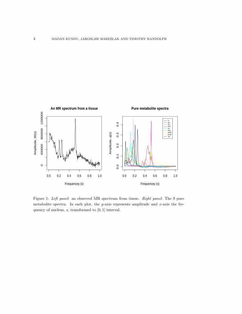
Figure 1: Left panel: an observed MR spectrum from tissue. Right panel: The 9 pure

metabolite spectra. In each plot, the y-axis represents amplitude and x-axis the fre-

quency of nucleus, s, transformed to [0, 1] interval.


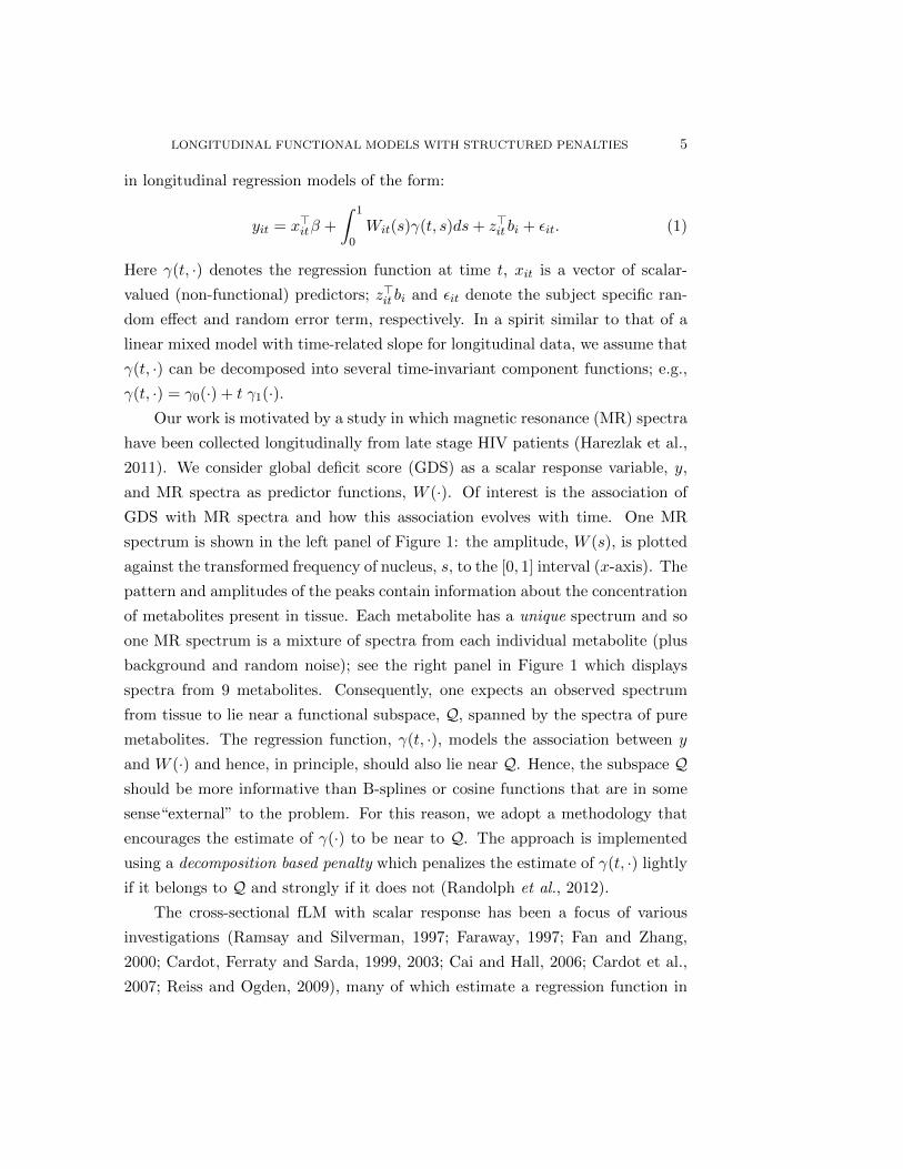
in longitudinal regression models of the form:

yit = x>itβ +

∫ 1

0Wit(s)γ(t, s)ds+ z>it bi + εit. (1)

Here γ(t, ·) denotes the regression function at time t, xit is a vector of scalar-

valued (non-functional) predictors; z>it bi and εit denote the subject specific ran-

dom effect and random error term, respectively. In a spirit similar to that of a

linear mixed model with time-related slope for longitudinal data, we assume that

γ(t, ·) can be decomposed into several time-invariant component functions; e.g.,

γ(t, ·) = γ0(·) + t γ1(·).Our work is motivated by a study in which magnetic resonance (MR) spectra

have been collected longitudinally from late stage HIV patients (Harezlak et al.,

2011). We consider global deficit score (GDS) as a scalar response variable, y,

and MR spectra as predictor functions, W (·). Of interest is the association of

GDS with MR spectra and how this association evolves with time. One MR

spectrum is shown in the left panel of Figure 1: the amplitude, W (s), is plotted

against the transformed frequency of nucleus, s, to the [0, 1] interval (x-axis). The

pattern and amplitudes of the peaks contain information about the concentration

of metabolites present in tissue. Each metabolite has a unique spectrum and so

one MR spectrum is a mixture of spectra from each individual metabolite (plus

background and random noise); see the right panel in Figure 1 which displays

spectra from 9 metabolites. Consequently, one expects an observed spectrum

from tissue to lie near a functional subspace, Q, spanned by the spectra of pure

metabolites. The regression function, γ(t, ·), models the association between y

and W (·) and hence, in principle, should also lie near Q. Hence, the subspace Qshould be more informative than B-splines or cosine functions that are in some

sense“external” to the problem. For this reason, we adopt a methodology that

encourages the estimate of γ(·) to be near to Q. The approach is implemented

using a decomposition based penalty which penalizes the estimate of γ(t, ·) lightly

if it belongs to Q and strongly if it does not (Randolph et al., 2012).

The cross-sectional fLM with scalar response has been a focus of various

investigations (Ramsay and Silverman, 1997; Faraway, 1997; Fan and Zhang,

2000; Cardot, Ferraty and Sarda, 1999, 2003; Cai and Hall, 2006; Cardot et al.,

2007; Reiss and Ogden, 2009), many of which estimate a regression function in


two steps. For example, Cardot, Ferraty and Sarda (2003) first perform principal

component regression (PCR), which projects the observed predictor curves onto

an empirical basis to obtain an estimate, then use B-splines to smooth the result.

Reiss and Ogden (2009) study several of these methods along with modifications

that include versions of PCR using B-splines and second-derivative penalties

(cf. (Ramsay and Silverman, 1997; Silverman, 2009)). Extensions of fLM have

been made towards generalized linear model with functional predictors (James,

2002; Muller and Stadtmuller, 2005) and quadratic functional regression (Yao

and Muller, 2010). We are interested in extending the fLM to a longitudinal

setting.

To our knowledge, the only published methods addressing the longitudinal

functional predictor framework are LPFR (Goldsmith et al., 2012) and LFPCR

(Gertheiss et al., 2013). The LPFR approach assumes the regression function in

(1) is independent of time and proceeds in three steps: use a truncated set of K-L

vectors to represent the predictor functions; express the regression function with

a spline basis; fit the longitudinal model using an equivalent mixed-model frame-

work that incorporates subject-specific random effects. In the LFPCR approach,

the predictor functions are first decomposed into visit- and subject-specific func-

tions accordingly via longitudinal functional principal component analysis (LF-

PCA) (Greven et al., 2011) and in a second step, longitudinal analysis is carried

out with the outcome of LFPCA. Both LPFR and LFPCR assume that the

regression function, γ(t, ·) remains constant over time. In contrast, we model

the coefficient function γ(t, ·) as a time-dependent linear combination of several

time-invariant component functions, γd(·)Dd=0, each of which is estimated via

a penalty operator that is informed by the structure of the data or a scientific

question.

Section 2 establishes notation for the model considered in this paper. In Sec-

tion 3.1, the concept of generalized ridge (Hoerl and Kennard, 1970) (or Tikhonov

(1963)) estimation is discussed. We review a decomposition-based penalty in Sec-

tion 3.2 and present how these estimates can be obtained as best linear unbiased

predictors (BLUP) through mixed model equivalence in Section 4.1. Expressions

for the precision of the estimates are derived in Section 4.2. In an Appendix

(Section 7) we present how our longitudinal penalized estimate, along with its


bias and precision, can be obtained, under some weak assumptions, in terms of

generalized singular vectors.

Numerical illustrations are provided by simulations in Section 5: Section 5.1

compares LPFR with the method proposed in this paper; Section 5.2 evaluates

the influence of sample size and the effect of using prior functional information;

Section 5.3 explores confidence band coverage probabilities; Section 5.4 evaluates

performance when only partial information is available. An application to real

MRS data using and a summary of our findings is presented in Section 5.5. The

methods discussed in this paper have been implemented in the R package refund

(Crainiceanu et al., 2012) via the peer() and lpeer() functions.

2 Statistical Model

We consider Ω = [0, 1], a closed interval in R, and let W (·) denotes a random

function in L2(Ω). Let Wit(·) denotes a predictor function from the ith subject

(i = 1, . . . , N) at the tth timepoint (t = t1, . . . , tni). Technically, an observed

predictor arises as a discretized sampling from an idealized function, and we

will assume that each observed predictor is sampled at the same p locations,

s1, . . . , sp ∈ [0, 1], with sampling that is appropriately regular and dense enough

to capture informative functional structure, as seen, for instance, in the MRS

data in Section 5.5. Let wit := [wit(s1), · · · , wit(sp)]> be the p × 1 vector of

values sampled from the realized function Wit(·). Then, the observed data are

of the form yit;xit;wit, where yit is a scalar outcome, xit is a K × 1 column

vector of measurements on K scalar predictors, and wit is the sampled predictor

from the ith subject at time t. Denoting the true regression function at time t

by γ(t, ·), the longitudinal functional regression outcome model of interest is

yit = x>itβ +

∫ 1

0Wit(s)γ(t, s)ds+ z>it bi + εit (2)

where, εit ∼ N(0, σ2ε ) and bi is the vector of r random effects pertaining to subject

i and distributed as N(0,Σbi). As usual we assume that zit is a subset of xit,

εit and bi are independent, εit and εi′t′ are independent whenever i 6= i′ or t 6= t′

or both, and bi and bi′ are independent if i 6= i′. Here x>itβ is the standard

fixed effect from K univariate predictors, z>it bi is the standard random effect and

8 MADAN KUNDU, JAROSLAW HAREZLAK AND TIMOTHY RANDOLPH∫ 10 Wit(s)γ(t, s)ds is the subject/time specific functional effect. We assume that

γ(t, ·) ∈ L2(Ω), for all t.

The functional structure, indexed by s, and time structure, indexed by t, have

somewhat unequal roles in our model, as we assume the longitudinal observations

are more limited in the amount of information relative to the densely-sampled s

index. For example, γ(t, s) may vary linearly with time, γ(t, s) = γ0(s)+tγ1(s), or

quadratically, γ(t, s) = γ0(s)+tγ1(s)+t2γ2(s). This is similar in spirit to a linear

mixed effects model with linear or quadratic time slope (see e.g., Fitzmaurice,

Laird and Ware, 2004). In general, we assume that γ(t, s) can be decomposed

into several time-invariant component functions γ0(s), · · · , γD(s) as

γ(t, s) = γ0(s) + f1(t)γ1(s) + . . .+ fD(t)γD(s)

where, f1, . . . , fD areD prescribed linearly independent functions of t and fd(0) =

0 for all d; the time component t enters into γ(t, s) through these terms. At t = 0,

γ(t, s) reduces to γ0(s) and has the obvious interpretation of a baseline regression

function pertaining to the sampling points s. When D = 0, γ(t, s) ≡ γ0(s) is

independent of t, a situation considered by Goldsmith et al. (2012). In general,

each f may be any function of t with f(0) = 0, e.g., f(t) = t or t exp(t). We can

rewrite the equation (2) as

yit = x>itβ +

∫ 1

0Wit(s)γ0(s) + f1(t)γ1(s) + . . .+ fD(t).γD(s)ds+ z>it bi + εit

The association of yit with Wit is modeled as a linear dependence on observations

at p sampling points, wit. In our approach, the (functional) structure is imposed

directly into the estimation of each γd = [γd(s1), . . . , γd(sp)]>, for d = 0, . . . , D

(as described in Section 3). Combining all n• =∑N

i=1 ni observations from the

N subjects obtained across all time points, we express the model as

y = Xβ +Wγ + Zb+ ε. (3)

Here, y = [y1t1 , · · · , y1tn1, . . . , y1tN , . . . , yNtnN ]> is a n• × 1 vector of all re-

sponses, X = [x>1t1 , · · · , x>1tn1

, · · · , x>1tN , · · · , x>NtnN

]> is an n• × K design ma-

trix pertaining to K univariate predictors, β is the associated coefficient vector,

γ = [γ>0 , γ>1 , · · · , γ>D]> is a (D+ 1)p×1 vector of functional coefficients, W is the

corresponding n• × (D + 1)p design matrix. Further, b is the rN × 1 vector of


random effects and Z is the corresponding n• × rN design matrix. The matrix

W has the structure

W =

W1

...

WN

Wi =

w>it1 f1(t1)w>it1 · · · fD(t1)w>it1

......

. . ....

w>itnif1(tni)w

>itni

· · · fD(tni)w>itni

3 Estimation of Parameters with a Penalty

Our approach builds on intuition from single-level functional regression that en-

courages an estimate of γ(·) to be in or near a “preferred” space via choice of

penalty operator (Randolph et al., 2012). To describe the effect of a general

penalty operator, L, it is useful to consider the familiar example of a Lapla-

cian penalty, L. The typical heuristic for this arises by viewing β as a function

whose local “smoothness” is informative. In this case, the term ||Lβ||2 penalizes

sharp changes in β. For our perspective, it is helpful to recall that the dominant

eigenvectors of L (those corresponding to the largest eigenvalues) are sharply os-

cillatory while the least-dominant eigenvectors are very smooth. Hence a linear-

algebraic view of this is that rather than penalizing sharp changes, smoothness in

the estimate is inherited from the eigenproperties of L. More specifically, struc-

ture in the estimate arises from the joint eigenproperties of X and L (as given

by the GSVD). In general, the least-dominant eigenvectors of a penalty L will

have the largest effect on the estimate. This property can be used to construct a

“preferred subspace” by defining a penalty L whose least-dominant (or perhaps

zero-associated) eigenvectors are preferred. The steps in PEER approach are

as follows: (1) Identify the functional space where W (·) is expected to belong

and treat this as a “preferred” space; (2) define a decomposition-based penalty

(see Section 3.2) that penalizes more when the estimate of γ falls into the non-

preferred space compared to preferred space. (3) Estimate γ(·) as a penalized

estimate. In our longitudinal setting, we encourage the estimates for each of the

γ0(·), · · · , γD(·) to be close to a preferred functional subspace. Our estimation

approach allows the preferred subspace to be different for each of the γd(·)’s. In

the longitudinal (or t) dimension, γ is more explicitly and severely constrained

by the choice of f1, . . . , fD.


3.1 Generalized Ridge Estimate

The model described in the previous section can be written as

y = Xβ +Wγ + ε∗, (4)

where ε∗ = Zb+ ε ∼ N(0, V ) and V = ZΣbZ>+σ2

ε I. Fore each d = 0, . . . , D, let

Ld be the penalty operator for γd and let λ2d be the associated tuning parameter.

The corresponding penalized estimates of β and γ are minimizers of:

||y −Xβ −Wγ||2V −1 + λ20||γ0||2L>0 L0

+ · · ·+ λ2D||γD||2L>DLD . (5)

Here we use the notation ||a||2B = a>Ba, where B is a symmetric, positive definite

matrix. A generalized ridge estimate of β and γ based on minimizing the above

expression is obtained as (see e.g., Ruppert, Wand and Carroll, 2003, p. 66)[β

γ

]= (C>V −1C +D)−1C>V −1y (6)

where, C = [X W ], D = blockdiag0, L>L and L = blockdiagλ0L0, · · · , λDLD.In the Appendix, we derive an expression for the generalized ridge estimate

γ explicitly in terms of the generalized singular value decomposition (GSVD)

components.

3.2 Decomposition based penalty

Let γd ≡ γLd,λd be the estimate obtained from the penalty operator Ld and tun-

ing parameter λ2d, for each d = 0, . . . , D. For example, Ld may denote Ip (a

ridge penalty) or a second-order derivative penalty (giving an estimate having

continuous second derivative). Alternatively, with prior knowledge about poten-

tially relevant structure in a regression function, a targeted decomposition-based

penalty can be defined in terms of a subspace defined by such structure (Randolph

et al., 2012). To be precise, if it is appropriate to impose scientifically-informed

constraints on the “signal” being estimated by γ, this prior may be implemented

by encouraging the estimate to be in or near a subspace, Q ⊂ L2(Ω).

Returning to our notation that reflects functional predictors observed at

p sampling points, we represent Q by the range of a p × J matrix Q whose

columns are q1, . . . , qJ . Consider the orthogonal projection PQ = QQ+ onto


the Range(Q), where Q+ is Moore-Penrose inverse of Q. Then a decomposition

penalty is defined as

LQ = φbPQ + φa(I − PQ) (7)

for scalars φa and φb. To see how LQ works, let γd be any estimate of γd.

When γd ∈ span(Q), we have LQγd = φbγd, but when γd /∈ span(Q), we have

LQγd = φaγd. The condition φa > φb imposes more penalty for γd /∈ span(Q)

compared to when γd ∈ span(Q). The weights φa and φb determine the relative

strength of emphasizing Q in the estimation process. Note, in particular, that

taking φa = φb results in a ridge estimate and that LQ is invertible, provided

φa and φb are nonzero. Some analytical properties for this family of penalized

estimates are discussed in Randolph et al. (2012).

4 Mixed model representation

Estimates of β and γ obtained by minimizing the expression in equation (5)

correspond to a generalized ridge estimate. In this section we aim to construct

an appropriate mixed model that minimizes the expression in equation (5). In

general, the penalty, L, is not required to be invertible but for simplicity this will

be assumed here. The mixed model approach provides an automatic selection of

tuning parameters λ1, · · · , λD. REML-based estimation of the tuning parame-

ters has been shown to perform as well as the other criteria and under certain

conditions it is less variable than GCV-based estimation (Reiss and Ogden, 2009).

4.1 Estimation of parameters

Using Henderson’s justification (Henderson, 1950), one can show that, for each

d = 0, . . . , D, the model y = Xβ + Wγ + ε∗ where, ε∗ ∼ N(0, V ) and γd ∼N(0, 1

λ2d(L>d Ld)

−1), minimizes the expression in equation (5) to obtain the BLUP.

Thus the generalized ridge estimate of β and γ correspond to the BLUP from

the following model:

y = Xβ +W ∗γ∗ + ε

where, W ∗ = [W Z], γ∗ = [γ> b>]> ∼ N [0,Σγ∗ ] and ε ∼ N(0, σ2ε I) with

Σγ∗ = blockdiag(L>L)−1, Σb and Σb = blockdiagΣb1 , · · · ,ΣbN .


This representation allows us to estimate fixed and functional predictors simply

by fitting a linear mixed model (e.g., using the lme() of the nlme package in R

or PROC MIXED in SAS).

4.2 Precision of Estimates

Our ridge estimate is the BLUP from an equivalent mixed model, hence the

variance of the estimate depends on whether the parameters are random or fixed.

Randomness of γ is a device used to obtain the ridge estimate while ε and b in

our case are truly random. With this in mind, we follow Ruppert, Wand and

Carroll (2003) and assume that the variance of the estimates is conditional on γ,

but not on b. The BLUP of β, γ and b can be expressed as (see e.g., Robinson,

1991; Ruppert, Wand and Carroll, 2003):

β =(X>V −1

1 X)−1

X>V −11 y γ = (L>L)−1W>V −1

1 (y −Xβ)

b = ΣbZ>V −1

1 (y −Xβ)

where V1 = V + W (L>L)−1W>. β is an unbiased estimator of β, but γ is not

unbiased. It is trivial to see that Cov(y|γ) = V . Thus, the variances of β and γ,

conditional on γ, are:

Cov(β|γ) =(X>V −1

1 X)−1

X>V −11 V V −1

1 X(X>V −1

1 X)−1

Cov(γ|γ) = AγV A>γ Aγ = (L>L)−1W>V −1

1 V1 −X(X>V −11 X)>V −1

1 (8)

To obtain the unconditional variance, one must replace V by V1 in the above

expressions, but this will overestimate the variance of the estimates. Expressions

for the predicted value of y and its variance are:

y = Xβ +Wγ + Zb Cov(y|γ) = AyV A>y

whereAy = [V1−WL>LW−ZΣbZ>−1X

(X>V −1X

)−1X>V −1+WL>LW>+

ZΣbZ>]V −1

1 .

Let, T = [1 f1(t) · · · fd(t)]⊗ IK . Then the discretized version of regression

function at time t is γ(t) = [γ(t, s1), · · · , γ(t, sK)] = Tγ. Therefore, the esti-

mate of γ(t) is γ(t) = T γ and the estimate of its variance is TCov(γ|γ)T>. The

smoothing parameters’ estimates are the ratios of the variance components in


the mixed model equivalence of the LongPEER model. The derivations above do

assume the knowledge of the variance components’ true values. In practice, these

variance components are estimated and the empirical versions of the regression

parameters are obtained (EBLUPs).

4.3 Selection of time-structure in γ(t, ·)

The proposed approach allows a flexible choice of the time structure to be in-

cluded in the regression function γ(t, ·). In practice, data and information to

estimate structure of the longitudinal observations (along the t index) are more

limited than the functional relationship along the s index. For example, whether

γ0(t, ·) + tγ1(t, ·) is sufficient or the more flexible γ0(t, ·) + tγ1(t, ·) + t2γ2(t, ·)is required is not known. The problem of choosing appropriate time-structure

in γ(t, ·) is similar, in principle, to that of choosing time structure in a linear

mixed-effects model (e.g., E(yit|bi) = β0 + β1 t or E(yit|bi) = β0 + β1 t+ β2 t2).

We propose two approaches to decide what the form of unknown regression func-

tion is: (a) Use of the AIC to compare different structures, and (b) Use of the

point-wise confidence band for the component functions: γ0(s), . . . , γD(s). If the

confidence band for any γd(s) contains zero in its entire domain, then such term

is dropped from the γ(t, s).

4.4 Selection of φa and φb for a decomposition penalty

We view φa and φb as weights of a tradeoff between preferred and non-preferred

subspaces and assume φa ·φb = constant. In the current implementation, we use

REML to estimate λd’s for a fixed value of φa, and do a grid search over the φa

values to jointly select the tuning parameters which maximize the information

criterion, such as AIC, based on the restricted maximum likelihood.

5 Simulation

We pursue several simulations to evaluate the properties of the LongPEER

method. The first simulation study (Section 5.1) compares the performance of

the LongPEER method with the LPFR approach. In the remaining simulation

studies, only the LongPEER method is considered. The purpose of the second


simulation study is to evaluate the influence of sample size and the contribution

of prior information about the functional structure (as determined by the tuning

parameters φa and φb in (7)) on the LongPEER estimate. In the third simulation

study, we evaluate the coverage probabilities of the confidence bands constructed

using the formula presented in Section 4.2. Finally, we evaluate the performance

of LongPEER estimate when information on some features is missing and the

results are summarized in Section 5.4. In all the simulation studies, the simu-

lated predictor functions resemble the MRS data. All results summarized in this

Section are based on 100 simulated datasets.

For each subject and visit, predictor functions were simulated independently.

Predictor functions were flat with bumps of varied widths at a number of pre-

specified locations. White noise was added to the predictor functions to account

for the instrumental measurement noise. These “bumpy” regression functions

were generated with bumps at some (but, not all) of the bump locations of the

predictor function. For the simulation in Section 5.1, the regression function is

assumed to be independent of time, whereas it varies with time in the simulation

of Section 5.2. For both the predictor and regression functions, 100 equi-spaced

sampling points in [0,1] are used.

For the decomposition penalty (7), the matrix Ld is defined as follows: 1)

select the discretized functions qj , j = 1, . . . , J spanning the “preferred” subspace

and 2) compute Ld = QQ+, where Q = col[q1, . . . , qJ ] and the vectors qPj are

discretized functions, defined to have a single bump corresponding to a region in

the simulated predictor functions; see Figure 2. The columns of Q need not be

orthogonal (cf., Figure 9).

Estimation error is summarized in terms of the mean squared error (MSE)

of the estimated regression function defined as ||γ − γ||2, where γ denotes the

estimate of γ. Further, MSE was decomposed into the trace of the variance

and squared norm of bias. We also calculated the sum of squares of prediction

error (SSPE) as ||y− y||2/N , where y denotes the estimate of the true (noiseless)

y. The estimates based on the proposed methods, including the LongPEER

estimate, were obtained as BLUPs from the mixed model formulation described

in Section 4.1.


5.1 Comparison with LPFR

As mentioned, LPFR estimates a regression function that does not vary with

time. Therefore, in the first set of simulations we generated outcomes using a

time-invariant regression function (i.e., γ(t, s) = γ0(s), for all t). The following

model was used to generate the outcome data for 100 individuals (i = 1, · · · , 100),

each at 4 timepoints (t = 0, 1, 2, 3):

yit = β0 +

∫ 1

0Wit(s)γ0(s)ds+ bi + εit, i = 1, · · · , 100, (9)

where, γ0(s) =∑h∈Hγ0

a0h exp

[−2500 ∗

(h− s100

)2].

The bumpy predictor functions were generated from the following equation

wit(s) =∑h∈H1

(ξ1h + c1h)exp

[−2500 ∗

(s− h100

)2]

(10)

+∑h∈H2

(ξ2h + c2h)exp

[−1000 ∗

(s− h100

)2]

+ (ξ31 + 0.9)exp

[−250 ∗

(s− 50

100

)2],

where c1h, c2h and a0h are defined in Table 1. ξ1h, h ∈ H1, ξ2h, h ∈ H2,and ξ31 were drawn independently from Uniform(0, 0.1). Also, β0 = 0.06, εit ∼N [0, (0.02)2] and bi ∼ N [0, (0.05)2].

Table 1: Values of c1h, c2h, a0h and a1h for generating predictor and regression function

in simulation studies in Sections 5.1, 5.2, 5.3 and 5.4.

h ∈ H1 h ∈ H2 h ∈ Hγ0 h ∈ Hγ1

h c1h h c2h h a0h h a1h

15 0.10 30 0.60 15 0.20 30 0.06

5 0.10 70 0.50 50 -0.15 70 -0.06

80 0.50 80 0.15

90 0.40

We applied both LPFR (using lpfr() available in the refund package in R

(Crainiceanu et al., 2012)) and the LongPEER method to the simulated data.


0.0 0.2 0.4 0.6 0.8 1.0

0.0

0.4

0.8

Columns of Q

s

0.0 0.2 0.4 0.6 0.8 1.0

−0.15

−0.05

0.00

0.05

0.10

0.15

0.20

s

γ 0

TrueLongPEER EstimateLPFR Estimate

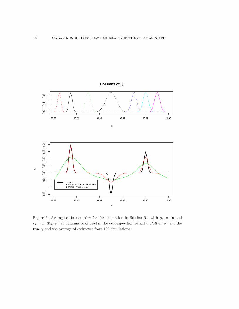
Figure 2: Average estimates of γ for the simulation in Section 5.1 with φa = 10 and

φb = 1. Top panel: columns of Q used in the decomposition penalty. Bottom panels: the

true γ and the average of estimates from 100 simulations.


Table 2: Estimation and prediction errors for LPFR and LongPEER estimates based

on 100 simulated datasets. The sample size is N = 100 and the number of longitudinal

observations is ni = 4.

LongPEER LPFR

MSE(γ0) 0.0323 0.2244

Trace of Variance(γ0) 0.0028 0.0490

||Bias(γ0)||2 0.0295 0.1754

SSPE of Y 1.1566 1.1535

To obtain the LPFR estimate, the dimension of both principal components for

predictor function and truncated power series spline basis for the regression func-

tion were set to 60. The columns of Q used to define LQ, for the LongPEER

estimate are plotted in the top panel of Figure 2. We used φa/φb = 10, a choice

motivated by our findings in Sections 5.2 and 5.4.

Table 2 displays the MSE and prediction error obtained for LongPEER and

LPFR estimates. The SSPE was similar for both methods (1.1566 and 1.1535),

however, the LongPEER estimate has smaller MSE. Both the bias and variance

are higher for the LPFR estimate and consequently it has the greater MSE. Fig-

ure 2 displays the estimates of the regression function. It should be emphasized

that any comparison of these methods is not entirely fair since LongPEER is de-

signed to exploit presumed structural information while LPFR is not. We note

also that the ability to exploit such information may be limited and so in this

simulation we used imprecise information about the shapes of features; see top

panel in Figure 2. Not surprisingly, performance is best for the feature at s = 0.15

where information about the shape was relatively precise. See also Section 5.4.

5.2 Simulation with a time varying regression function

Here the regression function varies parametrically with time. Lacking other func-

tional regression methods that estimate a time-varying regression function, we

only evaluated the performance of LongPEER. The primary goal was to assess

the effects of sample size, fraction of variance explained by the model, and the

relative contribution of external information (as determined by φa and φb in

equation 7) on estimate.


0.5 1.0 1.5 2.0 2.5 3.0

0.02

00.

030

0.04

00.

050

Average MSE(γ0)

log10(φa)

N=200, R2=0.9N=100, R2=0.9N=200, R2=0.6N=100, R2=0.6

0.5 1.0 1.5 2.0 2.5 3.0

0.00

20.

003

0.00

40.

005

0.00

6

Average MSE(γ1)

log10(φa)

N=200, R2=0.9N=100, R2=0.9N=200, R2=0.6N=100, R2=0.6

0.5 1.0 1.5 2.0 2.5 3.0

40

05

40

15

40

25

Average AIC (N=200, R2=0.9)

log10(φa)

0.5 1.0 1.5 2.0 2.5 3.0

19

60

19

65

19

70


log10(φa)

0.5 1.0 1.5 2.0 2.5 3.0

30

14

30

16

30

18

30

20


log10(φa)

0.5 1.0 1.5 2.0 2.5 3.0

14

76

.51

47

7.5

14

78

.51

47

9.5


log10(φa)

0.5 1.0 1.5 2.0 2.5 3.0

0.0

10

50

.01

15

Average SSPE

log10(φa)

N=200, R2=0.9N=100, R2=0.9N=200, R2=0.6N=100, R2=0.6

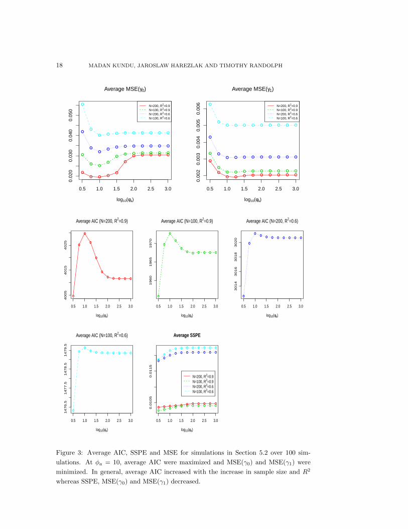
Figure 3: Average AIC, SSPE and MSE for simulations in Section 5.2 over 100 sim-

ulations. At φa = 10, average AIC were maximized and MSE(γ0) and MSE(γ1) were

minimized. In general, average AIC increased with the increase in sample size and R2

whereas SSPE, MSE(γ0) and MSE(γ1) decreased.


Without loss of generality, we set φb = 1 and vary φa on an exponential

scale. Larger values of φa indicate greater emphasis of prior information on the

estimation process. The model considered here is similar to that described in

Section 5.1 with the exception that γ(t, s) = γ0(s) + t γ1(s). The function γ0(s)

is defined in equation (10) and γ1(s) is of the form

γ1(s) =∑h∈Hγ1

a1h exp

[−2500 ∗

(h− s100

)2]

where the value of h and a1h are listed in Table 1 and β0 = 0.06. Realizations of

functional predictors were generated as described in section 5.1. For each simula-

tion, an appropriate σ2ε was chosen to ensure that the squared multiple correlation

coefficientR2 = s2y/[s

2y+σ

2ε ] is 0.6 and 0.9. Here, s2

y = 14

∑3t=0

1N−1

∑Ni=1 (yit − y.t)2

denotes the average sample variance in the set yit − εit : i = 1, · · · , N ; t =

0, · · · , 3 with y.t = 1N

∑Ni=1 yit.

We have repeated the simulation for four scenarios: (i) N = 100, R2 = 0.6;

(ii) N = 100, R2 = 0.9; (iii) N = 200, R2 = 0.6; and (iv) N = 200, R2 = 0.9.

Estimate of γ0 and γ1 were obtained using a decomposition penalty. The columns

of Q used to define LQ are plotted in the top panel of Figure 5. Results for AIC,

MSE and SSPE are displayed graphically in Figure 3. The standard deviation

of MSE were plotted in Figure 4. As the sample size and R2 increased, both

the MSE(γ0) and MSE (γ1) were decreased, providing empirical evidence that

the LongPEER estimates were consistent. In all four scenarios, MSE(γ0) was

minimized at φa = 10, it increased with φa up to φa = 100, and plateaued after

that. On the other hand, a decrease in MSE(γ1) is observed as φa increased up

to 10 and it plateaued thereafter. That is, an increase in φa up to 10 resulted in

improvement in estimation of both γ0 and γ1. However, φa beyond 10 resulted

in deterioration in performance of estimation for γ0; estimation performance for

γ1 remained almost unchanged. To understand this result, we need to compare

the plots of columns for Q matrix used in defining LQ with true γ0 and γ1 in

Figure 5: γ0 has peaks at s = 0.2, 0.5 and 0.8. and Q contains functions (colums)

representing peaks at these locations. However, the shape of the peak at s = 0.5

is different from that in γ0. Due to this difference in shape, as φa increased

from 10 to 100, the feature at s = 0.5 in γ0 became smaller leading to gradual

increase in MSE(γ0). On the other hand, γ1 has two features while Q contains


0.5 1.0 1.5 2.0 2.5 3.0

0.00

20.

006

0.01

0

Standard Deviation of MSE(γ0)

log10(φa)

N=200, R2=0.9N=100, R2=0.9N=200, R2=0.6N=100, R2=0.6

0.5 1.0 1.5 2.0 2.5 3.0

0.00

050.

0010

0.00

15

Standard Deviation of MSE(γ1)

log10(φa)

N=200, R2=0.9N=100, R2=0.9N=200, R2=0.6N=100, R2=0.6

Figure 4: Standard deviation of MSE for simulations in Section 5.2 over 100 simulations.

Standard deviation of MSE(γ0) and MSE(γ1) generally decrease with increasing sample

size and R2. MSE(γ0) and MSE(γ1) both decrease up to 101.25 and then plateau, except

for MSE(γ0) in the scenario with N = 200 and R2 = 0.9.

functions of very similar shape. Consequently, MSE(γ1) stabilizes after φa = 10.

Finally, note that the value of φa that maximized AIC also minimized MSE(γ0)

and MSE(γ1). This suggests that AIC can be used to guide the choice of φa while

setting φb at 1. In general, the choice of φa may be take as that which maximizes

AIC.

The average LongPEER estimate of γ0 and γ1 using a decomposition penalty

are displayed in Figure 5 with φa = 10 and φb = 1. For smaller sample sizes and

R2, the LongPEER estimate may: (a) oversmooth (i.e., negatively bias) the

estimated regression function at locations of a true feature, and (b) be positively

biased in locations corresponding to features in Q but where the true γ is zero.

However, by increasing the sample size to 200 and/or R2 to 0.9, we observe that

the average LongPEER estimate γ0(·) and γ1(·) approach the true functions.

5.3 Coverage probability

In this section, we used the simulation setup described in Section 5.2 with R2 =

0.9. The columns of Q matrix used in defining the decomposition penalty (7)


0.0 0.2 0.4 0.6 0.8 1.0

0.0

0.4

0.8

Columns of Q

s

0.0 0.2 0.4 0.6 0.8 1.0

−0.15

−0.10

−0.05

0.00

0.05

0.10

0.15

0.20

γ~0(.)

s

TrueMean Estimate(N=200, R2=0.9)Mean Estimate(N=100, R2=0.9)Mean Estimate(N=200, R2=0.6)Mean Estimate(N=100, R2=0.6)

0.0 0.2 0.4 0.6 0.8 1.0

−0.06

−0.04

−0.02

0.00

0.02

0.04

0.06

γ~1(.)

s

TrueMean Estimate (N=200, R2=0.9)Mean Estimate(N=100, R2=0.9)Mean Estimate(N=200, R2=0.6)Mean Estimate(N=100, R2=0.6)

Figure 5: Average estimates of the components of regression functions for simulations

described in Section 5.2 with φa = 10 and φb = 1. Top panel: columns of Q used in

defining a decomposition penalty. Middle and bottom panels: the average estimates of γ0

and γ1; these improve as N and/or R2 increase.


0.0 0.2 0.4 0.6 0.8 1.0

0.00.4

0.8

Columns of Q

s

0.0 0.2 0.4 0.6 0.8 1.0

−0.

2−

0.1

0.0

0.1

0.2

N=100 (Average coverage = 0.9218)

s

γ 0(s

)

0.0

0.2

0.4

0.6

0.8

1.0

Pro

port

ion

of c

over

age

TrueCoverage

0.0 0.2 0.4 0.6 0.8 1.0

−0.

10−

0.05

0.00

0.05

0.10


s

γ 1(s

)

0.0

0.2

0.4

0.6

0.8

1.0

Pro

port

ion

of c

over

age

TrueCoverage

0.0 0.2 0.4 0.6 0.8 1.0

−0.

2−

0.1

0.0

0.1

0.2


s

γ 0(s

)

0.0

0.2

0.4

0.6

0.8

1.0

Pro

port

ion

of c

over

age

TrueCoverage

0.0 0.2 0.4 0.6 0.8 1.0

−0.

10−

0.05

0.00

0.05

0.10


s

γ 1(s

)

0.0

0.2

0.4

0.6

0.8

1.0

Pro

port

ion

of c

over

age

TrueCoverage

Figure 6: Coverage probabilities of LongPEER estimates in 100 simulations with φa = 10

and φb = 1 discussed in section 5.3. Top panel: the columns of Q used in the decom-

position penalty. Middle and bottom panels: pointwise 95% confidence band (shaded

region) and coverage proportions (the dotted line) based on N = 100, and N = 400

subjects, respectively. The left column displays the cross-sectional function γ0(·) and

the right column the longitudinal function γ1(·). The horizontal line in each plot marks

the nominal coverage of 95%.


are displayed in the top panel of Figure 6. The middle and bottom panel shows

the confidence bands and the coverage probabilities obtained using φa = 10. The

95% confidence bands are constructed as Estimate ±1.96× (Standard Error).

When the sample size N increased, there was a notable improvement in coverage

of both γ0(·) and γ1(·). For N = 100, the coverage of γ1(·) by the confidence

bands was only around 81%. This confidence band under-coverage of γ1(·) is

caused by the comparatively larger bias in the estimation of γ1(·) with N = 100

(see Section 5.2 and Figure 5). The observed coverage increases with N : for

N = 400, the coverage is very close to 95%. We also explored the influence of φa

on the confidence band and coverage probability (not shown here). The higher

values of φa led to the confidence band shrinkage and this in turn resulted in

under-coverage of both γ0(·) and γ1(·).

5.4 Estimation in the presence of incomplete information

Since the LongPEER estimate uses external information in the estimation pro-

cess, it is of interest to evaluate its estimation performance when only partial

information is available. In this section, we use a simulation scenario similar to

that in Section 5.3, but now the penalty is defined without regard for information

about the peak at s = 0.5. As displayed in Figure 7, the LongPEER estimates

of γ0(s) has appropriate structure at s = 0.5, on average. Indeed as with an

ordinary ridge penalty, this structure is inherited from the empirical eigenvectors

of W (·). This highlights the advantage of an estimate obtained from the jointly-

determined eigenvectors of W (·) and L (see Appendix 7); the estimate depends

on the relative contributions W and L, controlled by the ratio of φa to φb.

The relative increase in the contribution of external information in the es-

timation process resulted in shrinkage towards zero at s = 0.5. The estimates

displayed in Figure 7 result from φb = φa = 1 (i.e., a ridge penalty) in the middle

panel, and φb = 1, φa = 100.75 in the bottom panel. For values of φa larger than

100.75, minimal changes in the estimates are observed.

5.5 MRS study application

We applied LongPEER to investigate potential associations of metabolite spec-

tra, obtained from basal ganglia, and the global deficit score (GDS) in a lon-


0.0 0.2 0.4 0.6 0.8 1.0

−0.

15−

0.05

0.05

0.10

0.15

0.20

True function

s

γ 0(s

)

TruePrior information

0.0 0.2 0.4 0.6 0.8 1.0

−0.

06−

0.04

−0.

020.

000.

020.

040.

06

True function

sγ 1

(s)

TruePrior information

0.0 0.2 0.4 0.6 0.8 1.0

−0.

15−

0.05

0.05

0.10

0.15

0.20

Estimated function [φa=1,φb=1 (Ridge estimate)]

s

γ 0(s

)

TrueEstimate(N=100)Estimate(N=200)

0.0 0.2 0.4 0.6 0.8 1.0

−0.

06−

0.04

−0.

020.

000.

020.

040.

06Estimated function [φa=1,φb=1 (Ridge estimate)]

s

γ 1(s

)


0.0 0.2 0.4 0.6 0.8 1.0

−0.

15−

0.05

0.05

0.10

0.15

0.20

Estimated function [φa=100.75, φb=1]

s

γ 0(s

)


0.0 0.2 0.4 0.6 0.8 1.0

−0.

06−

0.04

−0.

020.

000.

020.

040.

06

Estimated function [φa=100.75, φb=1]

s

γ 1(s

)


Figure 7: Top panel: true regression functions (solid lines) γ0(·) (left) and γ1(·) (right)

and 6 vectors spanning PQ (dashed lines). Middle panel: Average ridge-penalty estimate

from 100 simulations. Bottom panel: Average LongPEER estimate from 100 simulations

with PQ defined by the 6 vectors displayed in the top panel and φa = 100.75.


Table 3: Comparison of AIC for selection of scalar covariates, φa (φb = 1) and time

structure in γ(t, ·) in Section 5.5

Scalar covariates Time structure in γ(t, ·) φa AIC

Model 1 t γ0(t, ·) + tγ1(t, ·) 10 −395.2335

Model 2 Age, t γ0(t, ·) + tγ1(t, ·) 10 −405.2796

Model 3 Gender, t γ0(t, ·) + tγ1(t, ·) 10 −395.9040

Model 4 Race, t γ0(t, ·) + tγ1(t, ·) 10 −398.5607

Model 5 t, t2 γ0(t, ·) + tγ1(t, ·) + t2γ2(t, ·) 10 −394.5752

Model 6 t γ0(t, ·) + tγ1(t, ·) 100 −395.3670

0 1 2 3 4

01

23

4

Prediction performance

y

y~

0 1 2 3 4

−1.5

−0.5

0.5

1.0

1.5

Residual plot

y~

y~−y

Figure 8: Prediction performance of Model in equation (11). Left panel: observed GDS

score (y) and predicted value (y). Right panel: observed y and residuals (y − y).


0.0 0.2 0.4 0.6 0.8 1.0

−0

.20

.00

.20

.40

.60

.81

.0

γ0~

s

γ0~

CrGluNAANAAGScyllo

0.0 0.2 0.4 0.6 0.8 1.0

−0

.4−

0.3

−0

.2−

0.1

0.0

0.1

0.2

0.3

γ1~

s

γ1~

CrGluNAANAAGScyllo

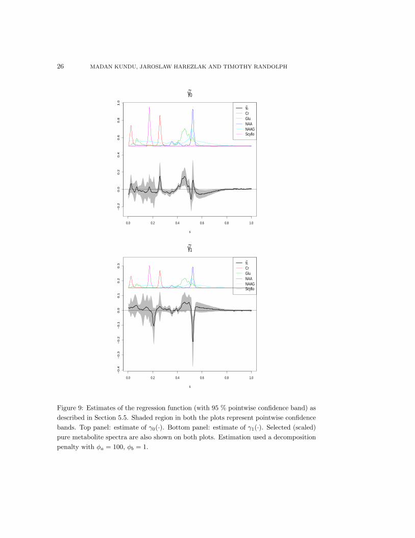
Figure 9: Estimates of the regression function (with 95 % pointwise confidence band) as

described in Section 5.5. Shaded region in both the plots represent pointwise confidence

bands. Top panel: estimate of γ0(·). Bottom panel: estimate of γ1(·). Selected (scaled)

pure metabolite spectra are also shown on both plots. Estimation used a decomposition

penalty with φa = 100, φb = 1.


gitudinal study of late stage HIV patients. Of particular interest is how such

an association evolves over time. The study description is available elsewhere

(Harezlak et al., 2011). We treat global deficit score (GDS) as our scalar con-

tinuous response variable and MR spectrum (sampled at K = 399 distinct fre-

quencies) as functional predictor. GDS is often used as a continuous measure

of neurocognitive impairment (e.g., Carey et al., 2004) and a large GDS score

indicates a high degree of impairment. The MRS spectra are comprised of pure

metabolite spectra, instrument noise and a background profile. We collected a

total of n• = 306 observations from N = 114 subjects. The longitudinal ob-

servations for each subject were within 3 years from baseline. The number of

observations per subject ranged from 1 to 5 with a median equal to 3. Spec-

tral information of 9 pure metabolites was used as prior information for the

LongPEER estimation. The pure metabolite spectra are: Creatine (Cr), Glu-

tamate (Glu), Glucose (Glc), Glycerophosphocholine (GPC), myo-Inositol (Ins),

N-Acetylaspartate (NAA), N-Acetylaspartylglutamate (NAAG), scyllo-Inositol

(Scyllo) and Taurine (Tau). These spectra are displayed in Figure 1. The de-

composition penalty, LQ, defined as in equation (7) where Q = [q1, · · · , q9], is a

matrix of dimension 9× 399.

Information available on demographic factors includes: age at baseline, gen-

der and race. We relied on AIC to choose (a) scalar covariates in the model,

(b) φa (while setting φb = 1) for defining decomposition based penalty LQ and

(c) the time structure of γ(t, ·). Based on the AIC (see Table 3), Models 1, 3, 5

and 6 are almost identical and appear to be better than the remaining models.

In these models, φa was selected to be either 10 or 100 and gender is the only

scalar covariate. Models 1 and 5 were different with respect to time structure in

γ(t, s). Although including γ2(t, ·) led to a marginal increase in AIC (−394.58 vs

−395.23), we did not observe any significantly non-zero region of γ2(t, ·), based

on pointwise 95% confidence intervals in Model 5. Models 1 and 6 were different

in terms of the φa. Use of smaller φa led to slight increase in AIC (−395.23 vs

−395.37). However, the interpretability of the estimates for γ0(·) and γ1(·) be-

came harder because of their increased wiggliness leading to the choice of Model

6.


Hence, we fit Model 1 (with φa = 100,φb = 1) as follows:

yit = β0 + β1 t+

∫ΩWit(s)γ(t, s)ds+ bi + εit, (11)

where γ(t, s) = γ0(s) + t γ1(s) and yit and Wit(·) are the GDS and the basal

ganglia spectrum for subject i at time t, respectively. We assume that εit ∼N(0, σ2

ε ) and bi is the subject-specific random intercept distributed as N(0, σ2b ).

The estimates were obtained as the BLUP from the mixed model formulation

described in Section 4.1 using L0 = L1 = LQ.

The estimates of λ (tuning parameter) associated with γ0(·) and γ1(·) were

1.152 and 2.242, respectively and the estimates of σ2ε and σ2

b were 0.0786 and

0.3332, respectively. The GDS score, fitted values and residual plot are displayed

in Figure 8 for the purpose of model checking. The residuals do not show an

obvious pattern indicating lack-of-fit of the proposed model.

Figure 9 displays the estimates of γ0(·) and γ1(·) with pointwise 95% con-

fidence bands. To aid interpretation, selected pure metabolite spectra are dis-

played. These figures reveal that γ0(·) (the “baseline” part of the regression

function) is different from zero at the locations where at least one of the pure

metabolites Cr, Glu, NAA, NAAG and Scyllo has a bump. Similarly, each non-

zero part of γ1(·) (the “longitudinal” part of the regression function) coincides

with bump locations of one or more pure metabolite profiles of Cr, Glu, NAA,

GPC and Ins.

Pointwise confidence intervals for γ0(·) and γ1(·) contain the 0 line over large

intervals. The estimated γ0 is significant in the region s ∈ (0.4, 0.5) ∪ (0.6, 0.8))

and estimated γ1 is significant in a region s ∈ (0.5, 0.6). To be precise, peaks

in both γ0(·) and γ1(·) are significant at locations where at least one of the

pure metabolite profiles NAA or Glu have bumps. The observation of negative

‘longitudinal’ effect of NAA is worth commenting; it suggests that GDS increases

as NAA concentration decreases in basal ganglia, a finding consistent with several

studies in which a reduced concentration of NAA is seen to be associated with

a decrease in neuronal mass (Christiansen et al., 1993; Lim and Spielman, 1997;

Soares and Law, 2009).

Finally, we considered other forms of f(t), such as exp(t) − 1 or log(t + 1).

When γ(t, ·) = γ0(t, ·) + [exp(t)− 1]γ1(t, ·) was compared with γ(t, ·) = γ0(t, ·) +


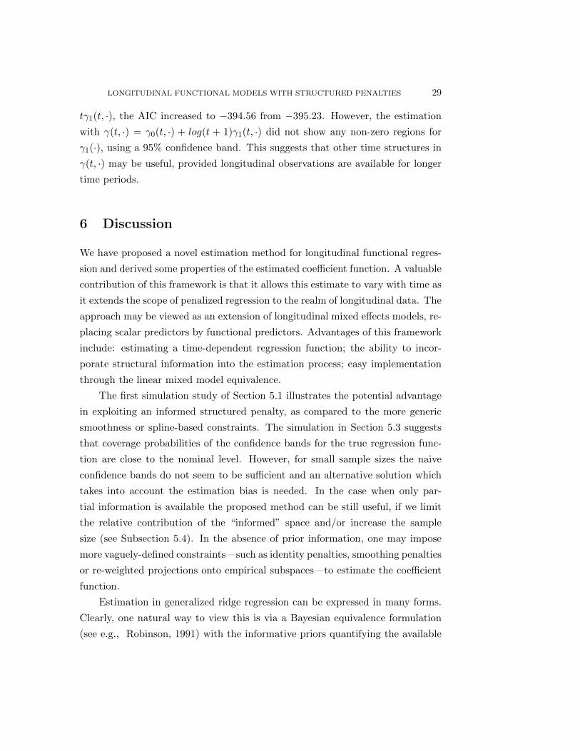
tγ1(t, ·), the AIC increased to −394.56 from −395.23. However, the estimation

with γ(t, ·) = γ0(t, ·) + log(t + 1)γ1(t, ·) did not show any non-zero regions for

γ1(·), using a 95% confidence band. This suggests that other time structures in

γ(t, ·) may be useful, provided longitudinal observations are available for longer

time periods.

6 Discussion

We have proposed a novel estimation method for longitudinal functional regres-

sion and derived some properties of the estimated coefficient function. A valuable

contribution of this framework is that it allows this estimate to vary with time as

it extends the scope of penalized regression to the realm of longitudinal data. The

approach may be viewed as an extension of longitudinal mixed effects models, re-

placing scalar predictors by functional predictors. Advantages of this framework

include: estimating a time-dependent regression function; the ability to incor-

porate structural information into the estimation process; easy implementation

through the linear mixed model equivalence.

The first simulation study of Section 5.1 illustrates the potential advantage

in exploiting an informed structured penalty, as compared to the more generic

smoothness or spline-based constraints. The simulation in Section 5.3 suggests

that coverage probabilities of the confidence bands for the true regression func-

tion are close to the nominal level. However, for small sample sizes the naive

confidence bands do not seem to be sufficient and an alternative solution which

takes into account the estimation bias is needed. In the case when only par-

tial information is available the proposed method can be still useful, if we limit

the relative contribution of the “informed” space and/or increase the sample

size (see Subsection 5.4). In the absence of prior information, one may impose

more vaguely-defined constraints—such as identity penalties, smoothing penalties

or re-weighted projections onto empirical subspaces—to estimate the coefficient

function.

Estimation in generalized ridge regression can be expressed in many forms.

Clearly, one natural way to view this is via a Bayesian equivalence formulation

(see e.g., Robinson, 1991) with the informative priors quantifying the available


scientific knowledge. In our formulation, the linear mixed model equivalence

provides an easy computational implementation as well as an automatic choice

of the tuning parameters using REML criterion. The GSVD provides algebraic

insight and a convenient way to derive the bias and variance expressions of the

estimates.

A possible extension of this work is to incorporate multiple functional pre-

dictors. For example, given two observed functional predictors W(1)t (·) and

W(2)t (·), consider two associated coefficient functions: γ(1)(t, ·) and γ(2)(t, ·).

We can express γ(1)(t, s) = γ(1)0 (s) + f

(1)1 (t)γ

(1)1 (s) + · · · + f

(1)d (t)γ

(1)d (s) and

γ(2)(t, s) = γ(2)0 (s) + f

(2)1 (t) + γ

(2)1 (s) + · · · + f

(2)d (t)γ

(2)d (s). Let W (1) and W (2)

represent design matrices for the two functional predictors. Then we can esti-

mate γ(1)(t, ·) and γ(2)(t, ·) by finding the BLUP estimate of γ(1) and γ(2) from

the mixed model: y = Xβ + W (1)γ(1) + W (2)γ(2) + Zb + ε. The simplified

formula for bias and variance derived in Section 7 still holds with an additional

assumption that (W (1))>V −1W (2) = 0.

As presented here, the method addresses models having a continuous scalar

outcome, but allowing for either binary or count responses is of interest. Indeed,

an important problem that arises in MRS data is that of understanding the

neurocognitive impairment status of HIV patients, defined as a binary variable,

based on functional predictors collected over time. Estimation in these general

settings appears to be possible with the proposed framework.

Acknowledgment: The authors thank Dr. B. Navia who provided the MRS

data used as an example in the manuscript. Partial research support was provided

by the National Institutes of Health grants U01-MH083545 (JH), R01-CA126205

(TR) and U01-CA086368 (TR).

7 Connection with the GSVD

We provide the derivation of a LongPEER estimate using the GSVD. This can

be viewed as an extension of the estimation discussed by Randolph et al. (2012)

in two ways: we allow for a general covariance matrix V (for y) and we extend

the penalty operator to apply across multiply-defined domains, L0, . . . , LD.

After some algebra, the generalized ridge estimate in (6) for γ can be ex-


pressed as

γ = −A1X>V −1y +A2W

>V −1y

where

A>1 = (X>V −1X)−1X>V −1W [W>V −1W + L>L−W>V −1X(X>V −1X)−1X>V −1W ]−1

A2 = W>V −1W + L>L−W>V −1X(X>V −1X)−1X>V −1W

When X = 0 (a situation without any scalar predictors) or X>V −1W = 0 the

generalized ridge estimation of γ can be put into a PEER estimation framework

in terms of GS vectors, as discussed below.

WithX = 0 orX>V −1W = 0, the γ reduces to [W>V −1W+L>L]−1W>V −1y.

Moreover, in this case generalized ridge estimate of β becomes [X>V −1X]−1X>V −1y.

Now, if we transform W := V −1/2W and y := V −1/2y, we can rewrite L as

L = λ0 blockdiag

L0,

λ1

λ0L1, · · · ,

λDλ0LD

= λ0L

s

Here, Ls can be interpreted as a scaled L where scaling is done for all the tuning

parameters associated with the ‘longitudinal’ part of the regression function with

respect to the ‘baseline’ tuning parameter.

Set p = (D + 1)p, let m denote the number of rows in L and set c =

dim[Null(L)]. Further, assume that n• ≤ m ≤ p ≤ m + n• and the rank of the

(n• + m) × p matrix [W> (Ls)>]> is p. The following describes the GSVD of

the pair (W , Ls): there exist orthogonal matrices U and V, a nonsingular G and

diagonal matrices S and M such that

W = USG−1 S = [0 S] S = blockdiagS1, Ip−m

Ls = VMG−1 M = [M 0] M = blockdiagIp−n• , M1

Submatrices S1 and M1 have ` = n• +m− p diagonal entries ordered as

0 < σ1 ≤ σ2 ≤ · · · ≤ σ` < 1

0 > µ1 ≥ µ2 ≥ · · · ≥ µ` > 1where, σ2

k + µ2k = 1, k = 1, . . . , `

Here, the columns gk of G are the GS vectors determined by the GSVD

of the pair (W , Ls). Denote the columns of U and V by uk and vk, respec-

tively. Now, it can be shown that [W>V −1W +L>L]−1W>V −1 = [W>V −1W +


λ20(Ls)>Ls]−1W>V −1 = G(S>S + λ2

0M>M)−1G> W>V −1/2 and consequently,

γ can be expressed as

γ = G(S>S+λ20M>M)−1S>U>y =

p−c∑k=p−n•+1

σ2k

σ2k + λ2

0µ2k

1

σku>k ygk+

p∑k=p−c+1

u>k ygk

Further, the bias and variance can be expressed as

Bias[γ] = (I −W#W )γ = G(S>S + λ20M>M)−1(λ2

0M>M)G−1

=∑p−n•

k=1 gkg>k γ +

∑p−ck=p−n•+1

λ20µ2k

σ2k+λ20µ

2kgkg>k γ

V ar[γ] = W#V (W#)> = G(S>S + λ20M>M)−1S>S(S>S + λ2

0M>M)−1G>

=∑p−c

k=p−n•+1σ2k

(σ2k+λ20µ

2k)2gkg>k +

∑pk=p−c+1 gkg

>k

where, W# = [W>V −1W + L>L]−1W>V −1 and gk denotes the kth column

of G−T = (G−1)> = (G>)−1. Further, we can express bias as [W>V −1W +

L>L]−1L>Lγ which means γ will be unbiased only when γ ∈ Null(L).

For estimates obtained using this technique, the bias and variance can be

expressed in terms of generalized singular vectors, provided the assumption of

X>V −1W = 0 applies. In this case, one can show that β is simply the generalized

least squares estimate from the linear model y = Xβ+ε∗, and γ is the generalized

ridge estimate from y = Wγ + ε∗ with penalty L. That is, β is estimated as if

Wγ were not present, and γ is estimated as if Xβ were not present.

Bibliography

Bjorck, A. (1996). Numerical methods for least square problems, 1st edition.

Philadelphia: SIAM.

Brumback, B. and Rice J. (1998). Smoothing spline models for the analysis of

nested and crossed samples of curves. Journal of American Statistical Associ-

ation 93(443), 961–976.

Cai, T. and Hall, P. (2006). Prediction in functional linear regression. The Annals

of Statistics 34(5), 2159–2179.

Cardot, H., Ferraty, F. and Sarda. P. (1999). Functional linear model. Statistics

and Probability Letters 45(1), 11–22.

Cardot, H., Ferraty, F. and Sarda, P. (2003). Spline estimators for the functional

linear model. Statistica Sinica 13, 571–591.

Cardot, H.,Crambes, C., Kneip, A. and Sarda, P. (2007). Smoothing splines esti-

mators in functional linear regression with errors-in-variables. Computational

Statistics Data Analysis 51(10), 4832–4848.

Carey, C., Woods, S., Gonzalez, R., Conover, E., Marcotte, T., Grant, I. and

Heaton, R. (2004). Predictive validity of global deficit scores in detecting neu-

ropsychological impairment in HIV infection. Journal of Clinical and Experi-

mental Neuropsychology 26(3), 307–319.

Christiansen, P., Toft, P., Larsson, H., Stubgaard, M. and Henriksen, O. (1993).

The concentration of N-acetyl aspartate, creatine + phosphocreatine, and

choline in different parts of the brain in adulthood and senium. Magnetic res-

onance imaging 11(6), 799–806.

33


Crainiceanu, C., Reiss, P., Goldsmith, A., Huang, L., Huo, L. and Scheipl F.

(2012). refund: Regression with Functional Data (R package version 0.1-6).

[http://CRAN.R-project.org/package=refund].

Di, C., Crainiceanu, C., Caffo, B. and Punjabi, N. (2009). Multilevel functional

principal component analysis. Annals of Applied Statistics 4, 458–288.

Engl, H. W., Hanke, M. and Neubauer, A. (2000). Regularization of Inverse

Problems, Klewer Academic Publishers.

Fan J., and Zhang, J. (2000). Two-step estimation of functional linear models

with applications to longitudinal data. Journal of the Royal Statistical Society:

Series B (Statistical Methodology) 62(2), 303–322.

Faraway, J. (1997). Regression analysis for a functional response. Technometrics

39(3), 254–261.

Fitzmaurice, M., Laird, G. and Ware, J. (2004). Applied Longitudinal Analysis,

1st edition. Wiley Series in probability and statistics.

Gertheiss, J., Goldsmith, J., Crainiceanu, C., and Greven, S. (2013). Longi-

tudinal scalar-on-functions regression with application to tractography data.

Biostatistics 14(3), 447–461.

Goldsmith, J., Bobb, J., Crainiceanu, C., Caffo, B. and Reich, D. (2011). Penal-

ized functional regression. Journal of Computational and Graphical Statistics

20(4), 830–851.

Goldsmith, J., Bobb, J., Crainiceanu, C., Caffo, B. and Reich, D. (2012). Lon-

gitudinal penalized functional regression for cognitive outcomes on neuronal

tract measurements. Journal of the Royal Statistical Society: Series C (Ap-

plied Statistics) 61(3), 453–469.

Golub G. and Van-Loan C. (1996) Matrix computations, Baltimore: John Hop-

kins University Press.

Greven, S., Crainiceanu, C., Caffo, B. and Reich, D. (2011). Longitudinal func-

tional principal component analysis. Recent Advances in Functional Data Anal-

ysis and Related Topics, 1st Edition. Physica-Verlag HD pp.149–154.

http://CRAN.R-project.org/package=refund


Guo,W. (2002). Functional mixed effects models. Biometrics 58(1), 121–128.

Hall, P., Poskitt, D., and Presnell. B. (2001). A functional data-analytic approach

to signal discrimination. Technometrics 43(1), 1–9.

Harezlak, J., Buchthal, S., Taylor, M., Schifitto, G., Zhong, J., Daar, E., Alger,

J., Singer, E., Campbell, T. and Yiannoutsos, C. (2011). Persistence of HIV-

associated cognitive impairment, inflammation, and neuronal injury in era of

highly active antiretroviral treatment. AIDS 25, 625–633.

Henderson,C. (1950). Estimation of genetic parameters (abstract). Annals of

Mathematical Statistics 21(1).

Hoerl, A.E. and Kennard, R.W. (1970). Ridge Regression: Biased Estimation for

Nonorthogonal Problems. Technometrics 12(1), 55–67.

James, G. (2002). Generalized linear models with functional predictors. Journal

of the Royal Statistical Society: Series B (Statistical Methodology) 64(3), 411–

432.

Lim, K. and Spielman, D. (1997). Estimating NAA in cortical gray matter

with applications for measuring changes due to aging. Magnetic resonance in

medicine 37(3), 372–377.

Morris, J. and Carroll, R. (2006). Wavelet-based functional mixed models. Jour-

nal of the Royal Statistical Society: Series B (Statistical Methodology) 68(2)

179–199.

Muller, H. (2005). Functional modelling and classification of longitudinal data.

Scandinavian Journal of Statistics 32(2), 223–240.

Muller, H. and Stadtmuller, U. (2005). Generalized functional linear models. The

Annals of Statistics 33(2), 774–805.

Paige, C. and Saunders, M. (1981). Towards a generalized singular value decom-

position. SIAM Journal on Numerical Analysis 18(3), 398–405.

Phillips, D. L. (1962), A technique for the numerical solution of certain integral

equations of the first kind, J. Associat. Comput. Mach., 9, 84–97.


Ramsay, J. and Dalzell, C. (1991). Some tools for functional data analysis. Jour-

nal of the Royal Statistical Society. Series B (Methodological) 53(3), 539–572.

Ramsay, J. and Silverman, B. (1997). Functional Data Analysis, 1st edition.

Springer-Verlag, Berlin.

Randolph, T., Harezlak, J. and Feng, Z. (2012). Structured penalties for func-

tional linear models – partially empirical eigenvectors for regression. Electronic

Journal of Statistics 6, 323–353.

Reiss, P. and Ogden, R. (2009). Smoothing parameter selection for a class of

semiparametric linear models. Journal of the Royal Statistical Society: Series

B (Statistical Methodology) 71(2), 505–523.

Robinson, G. (1991). That blup is a good thing: the estimation of random effects.

Statistical Science 6(1), 15–32.

Ruppert, D., Wand, M. and Carroll, R. (2003). Semiparametric Regression, 1st

edition. Cambridge Series in Statistical and Probabilistic Mathematics.

Salganik, M. and Wand, M. and Lange, N. (2004). Comparison of Feature Signif-

icance Quantile Approximations. Australian & New Zealand Journal of Statis-

tics 46(4), 569–581.

Silverman, B.W. (1996). Smoothed functional principal components analysis by

choice of norm. Annals of Statistics 24,, 1–24.

Soares, D. and Law, M. (2009). Magnetic resonance spectroscopy of the brain:

review of metabolites and clinical applications. Clinical radiology 64(1), 12–21.

Tikhonov, A. N. (1963), Solution of incorrectly formulated problems and the

regularization method, Dokl. Akad. Nauk SSSR, 151(3), 501–504 (in Russian);

English transl.: Soviet Math. Dokl., 4(4), 1035–1038.

Van-Loan, C. (1976). Generalizing the singular value decomposition. SIAM Jour-

nal on Numerical Analysis 13(1), 76–83.

Yao, F. and Muller, H. (2010). Functional quadratic regression. Biometrika

97(1), 49–64.


Department of Biostatistics

Indiana University Fairbanks School of Public Health

E-mail: [email protected]

E-mail: [email protected]

statistica sinica (2013): preprintstatistica sinica (2013): preprint 1 longitudinal functional...

Documents