Generalized staining algorithm for seismic modeling and migration

Qihua Li1 and Xiaofeng Jia1

ABSTRACT

The staining algorithm is introduced to improve the signal-to-noise ratio (S/N) of poorly illuminated subsurface structures inseismic imaging. However, the amplitudes of the original andthe stained wavefield, i.e., the real and the imaginary wavefields,differ by several orders of magnitude, and the waveform of thestained wavefield may be greatly distorted. We have developed ageneralized staining algorithm (GSA) to achieve amplitude pres-ervation in the stained wavefield. The real wavefield and thestained wavefield propagate in the same velocity model. A sourcewavelet is used as the source of the real wavefield; however, thereal wavefield is extracted from the stained area as the source ofthe stained wavefield. The GSA maintains some properties of the

original staining algorithm. The stained wavefield is synchron-ized with the real wavefield, and it contains only information rel-evant to the target region. By imaging with the stained wavefield,we obtain higher S/Ns in images of target structures. The mostsignificant advantage of our method is the amplitude preservationof the stained wavefield, which means that this method could po-tentially be used in quantitative illumination analysis and velocitymodel building. The GSA could be adopted easily for frequency-domain wavefield propagators and time-domain propagators.Furthermore, the GSA can generate any number of stained wave-fields. Numerical experiments demonstrate these features of theGSA, and we apply this method in target-oriented modeling andimaging as well as obtaining amplitude-preserved stained wave-fields and higher S/Ns in images of target structures.

INTRODUCTION

In general, seismic migration is a wave propagation-based processthat focuses reflections and diffractions and yields seismic images ofsubsurface areas. Migration plays a significant role in the processingof seismic data, and it is reliable and effective for resolving mostsubsurface structures. However, the limited acquisition geometry,overburden complexity, and the reflector dip angle may result in poorillumination of a subsurface target (Xie et al., 2006), which is prob-lematic for seismic imaging. Subsalt areas are among the mostproblematic areas for seismic prospecting. During wave propagation,amplitude loss and defocusing occur at each transmission through thehighly reflective salt boundaries (Leveille et al., 2011). The conse-quent amplitude loss, defocusing, and the weak reflectivity of thereflector result in a reduction in energy below the salt (Jackson et al.,1994; Muerdter and Ratcliff, 2001; Leveille et al., 2011; Liu et al.,2011). In such a poorly illuminated area, the amplitude of the signal iseven weaker than local multiples and scattered noise, which is de-structive to the image in most cases.

Many approaches have been proposed to improve the image qual-ity of weakly illuminated regions. Acquisition aperture correction inthe local angle domain (Cao and Wu, 2009) enhances the imageamplitude significantly. Illumination compensation for subsalt im-aging (Gherasim et al., 2010; Shen et al., 2011; Yang et al., 2012) isused to improve seismic wave signals in subsalt areas. The propa-gation wavepaths of multiple reflections are different from those ofthe primary reflections; therefore, multiples may be used to enhancesignals from poorly illuminated subsalt areas. Multiple scatteredwaves are used to image subsalt structures that are not sufficientlyilluminated by primary waves (Guitton, 2002; Malcolm et al.,2008). Liu et al. (2011) modify the conventional reverse time mi-gration (RTM) methodology by using multiples as constructive re-flection energy for imaging. An accurate velocity model facilitatesthe generation of good images, and therefore model-building tech-nology can greatly improve images of weakly illuminated areas(Fliedner et al., 2007; Liu et al., 2007; Mosher et al., 2007; Wanget al., 2008; Ji et al., 2011). In particular, Tang and Biondi (2011)

Manuscript received by the Editor 22 November 2015; revised manuscript received 19 September 2016; published online 22 November 2016.1University of Science and Technology of China, Laboratory of Seismology and Physics of Earth’s Interior, School of Earth and Space Sciences, Hefei, China.

E-mail: xjia@ustc.edu.cn.© 2017 Society of Exploration Geophysicists. All rights reserved.

T17

GEOPHYSICS, VOL. 82, NO. 1 (JANUARY-FEBRUARY 2017); P. T17–T26, 13 FIGS.10.1190/GEO2015-0652.1

Dow

nloa

ded

12/1

0/16

to 2

11.8

6.15

8.59

. Red

istr

ibut

ion

subj

ect t

o SE

G li

cens

e or

cop

yrig

ht; s

ee T

erm

s of

Use

at h

ttp://

libra

ry.s

eg.o

rg/

propose a target-oriented strategy for efficient wave-equation mi-gration velocity analysis of complex geologic settings.The staining algorithm is a processing technique used in seismic

migration that improves the signal-to-noise ratio (S/N) of poorlyilluminated areas (Chen and Jia, 2014) by muting target-unrelatedinformation from the migration results. The concept of the stainingalgorithm was inspired by a method in developmental biology calledfate mapping (Dale and Slack, 1987; Gilbert, 2000; Ginhoux et al.,2010). With the staining algorithm, when the seismic wavefrontreaches the “stained” target structure, reflection and transmissionoccur normally, but will be automatically labeled and traced in sub-sequent propagation. Thus, a stained wavefield is generated in addi-tion to the real wavefield. The stained wavefield is synchronized withthe real wavefield, but it includes only responses relevant to thestained structure. When a stained wavefield is used, nontarget infor-mation, including signals and noise, is muted from the migrationresults. Therefore, the S/N of the target structures is improved. Thestaining algorithm is regarded as a wavefield reconstruction strategythat is closely related to redatuming methods (Mulder, 2005). Thestaining algorithm is adaptable to most time–space-domain propaga-tors and is easy to implement. The complex-domain acoustic-waveequation is used in the original staining algorithm. Consequently, theamplitude of the original stained wavefield is several orders of mag-nitude smaller than that of the real wavefield, and thewaveform of theoriginal stained wavefield is greatly distorted. Therefore, the ampli-tude of the image from the original stained wavefield is several ordersof magnitude smaller than the RTM image.Preservation of the amplitude information is one of the key

considerations in seismic data processing. In the past few decades,efforts have been made to obtain accurate phase and amplitude in-formation for seismic modeling and imaging. Kirchhoff migration(Carter and Frazer, 1984; Gray, 1986; McMechan and Fuis, 1987;Keho and Beydoun, 1988) is used in wavefield extrapolation andseismic migration to image steeply dipping reflectors. Gaussianbeams were introduced to construct the Green’s function for wave-field extrapolation (Cerveny and Psencik, 1983; Wapenaar et al.,1989; Hill, 1990). Kirchhoff migration and the Gaussian beammethod are based on ray theory. However, solving wave equationsdirectly has an advantage for calculating the amplitude. Comparedwith one-way wave equation-based methods (Ristow and Ruhl,1994; Mulder and Plessix, 2004), full-wave equation-based meth-ods (Baysal et al., 1983; McMechan, 1983; Mulder and Plessix,2004) represent the amplitude information more accurately. DeBruin et al. (1990) determine the reflectivity of subsurface mediaby eliminating the contributions of the source, the downgoing wave-field propagator, and the upgoing reflected wavefield propagator tothe surface shot record based on the monochromatic acoustic 2Dforward model. Tarantola (1984a) solves the inversion problem inthe acoustic approximation of seismic reflection data based on thegeneralized least-squares criterion. Pseudooffset migration was in-troduced in the converted-wave prestack time-migration method toobtain amplitude-preserved images from anisotropic media (Zhangand Liu, 2008).In this paper, we reconstruct the stained wavefield in the model-

ing portion of the complex-domain staining algorithm (CDSA) andmodify the amplitudes and the waveforms of the stained wavefield.Our method maintains the correspondence between the stainedwavefield and the subsurface target structures. We apply this newstaining algorithm to RTM and obtain high-S/N images of weakly

illuminated structures. A stained wavefield with correct amplitudeinformation is potentially useful in other fields of seismic dataprocessing, such as velocity model building and quantitative illumi-nation analysis.

WAVE EQUATION IN THE COMPLEX DOMAIN

The conventional staining algorithm is based on the constant-den-sity full-acoustic-wave equation in the complex domain (O’Connelland Budiansky, 1978; Pujol, 2003; Baev, 2013, 2015; Chen and Jia,2014), given by

∂2ðp̄þ i ~pÞ∂t2

¼ ðv̄þ i ~vÞ2Δðp̄þ i ~pÞ þ s̄; (1)

whereΔ is the Laplace operator, the overbar denotes the real part, andthe tilde denotes the imaginary part of all variables. Accordingly, p̄refers to the real wavefield and ~p refers to the stained wavefield; v̄refers to the real-velocity model and ~v refers to the stained area. Thefunction ~v is set to be zero in nonstained areas, and in the stained area,~v → 0. Here, s̄ is the real source. Separating the real and the imagi-nary parts of equation 1 and neglecting the higher order infinitesimalterms 2v̄ ~vΔ ~p and ~v2, we obtain

∂2p̄∂t2

¼ v̄2Δp̄þ s̄ (2)

∂2 ~p∂t2

¼ v̄2Δ ~pþ ~s; (3)

~s ¼ 2v̄ ~vΔp̄; (4)

where ~s is regarded as the virtual source of the stained wavefield. Thetemporal spectrum of solution to equations 3 and 4 is

Fð ~pÞ ¼ 2k2ZZZ

~v≠0G

~vv̄p̄dV; (5)

where G is the Green’s function for equation 3, F denotes Fouriertransforms, and k denotes the wavenumber. Equation 5 is similar tothe Born modeling equation

δp ¼ 2k2ZZZ

δv≠0Gδvv0

podV; (6)

where δv refers to the velocity perturbation, v0 is the velocity model,po is the background wavefield, and δp is the scattered wavefield.Equation 5 is equivalent to equation 6; therefore, mathematically, thestained wavefield in the CDSA is essentially a scattering wavefieldfor a very small velocity perturbation. Note that in the CDSA, the realwavefield p̄ is regarded as the background wavefield; therefore,higher order scattering is also generated.We find that the real source wavelet s̄ and the virtual source ~s

propagate independently in the same velocity model v̄. From equa-tions 2 to 4, we know that s̄ only contributes to p̄, and ~s correspondsto ~p. The function ~p has no effect on p̄; however, as equation 4

T18 Li and Jia

Dow

nloa

ded

12/1

0/16

to 2

11.8

6.15

8.59

. Red

istr

ibut

ion

subj

ect t

o SE

G li

cens

e or

cop

yrig

ht; s

ee T

erm

s of

Use

at h

ttp://

libra

ry.s

eg.o

rg/

shows, p̄ provides the source for ~p. The virtual source term is de-fined by ~v and p̄. These relationships indicate that the stained wave-field is only excited when wavefronts of the real wavefield reach thestained area.The amplitude of the real wavefield is usually much larger than

that of the stained wavefield. Moreover, ~s is equal to 2v̄ ~vΔp̄; there-fore, the waveform of the stained wavefield is related to Δp̄. Con-sequently, compared with the real wavefield, the waveform of thestained wavefield is greatly distorted. The virtual source ~s must bemodified to obtain an amplitude-preserved stained wavefield thathas the same amplitude and waveform as the real wavefield.

AMPLITUDE PRESERVATION OF THE STAINEDWAVEFIELD

To obtain an amplitude-preserved stained wavefield, we constructthe equations for the real and the stained wavefields as

∂2p̄∂t2

¼ v̄2Δp̄þ s̄; (7)

∂2 ~p∂t2

¼ v̄2Δ ~p; (8)

~pjD¼1 ¼ p̄; (9)

D ¼�1; ~v ≠ 0

0; ~v ¼ 0: (10)

Equations 9 and 10 are the boundary conditions. Note that in thegeneralized staining algorithm (GSA), D labels the stained area in-stead of ~v. In the CDSA, a small value is assigned to ~v at the stainedarea; in the GSA, we define D ¼ 1 at the stained area and D ¼ 0

otherwise. In the CDSA, p̄ and ~p are the real and imaginary parts ofthe complex-valued wavefield p, respectively. However, in theGSA, ~p propagates independently from p̄ after the complete sourceinjection, which is the only connection between the two wavefields.The Kirchhoff integral (Wiggins, 1984; Docherty, 1991) gives the

solution to equation 7 as

1

4π

Zdτ

ID¼1

�Gðr; r 0 0; t; τÞ ∂p̄ðr

0 0; τÞ∂n

− p̄ðr 0 0; τÞ ∂Gðr; r0 0; t; τÞ

∂n

�dS

−Z

dτZZZ

Vcs̄ðr 0; τÞGðr; r 0; t; τÞdr 03 ¼ 0; (11)

p̄ðr; tÞ ¼ 1

4π

Zdτ

ZZZVc

s̄ðr 0; τÞGðr; r 0; t; τÞdr 03; (12)

where r 0 refers to the location of the source in volume Vc, r 0 0 refersto the vector from the origin to the integration point on S, r refers tothe spatial location outside of volume Vc, τ is the time at which thewavefield is observed, D ¼ 1 is the boundary of volume Vc, and Gis the Green’s function. The Kirchhoff integral enables us to recon-struct the wavefield on one side of a closed surface with sources onthe other side through calculating the surface integral in equation 11using the surface wavefield. The Kirchhoff integral requires p̄ and∂p̄∕∂n at the boundary of Vc to reproduce the real wavefield p̄ðrÞ.When the stained area D ¼ 1 is a boundary with a proper thickness,the first-order partial derivative ∂~p∕∂n can be determined accuratelyby equation 9. In this situation, the boundary is actually an area, andthe first-order partial derivative ∂~p∕∂n is determined anywherewithin the area except for the boundary of the area.The required thickness depends on the propagator. Assume that

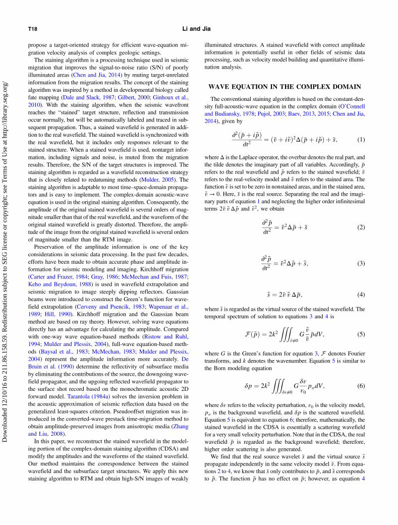
an h-order spatial accuracy explicit FD propagator is used for thestained wavefield propagation. The first-order partial derivative∂~p∕∂n is determined by the previous wavefield on h∕2 grid pointsnearby in direction n. This means that given the wavefield at theboundary with thickness of ðh∕2Þ − 1 grid intervals, ∂~p∕∂n can bedetermined accurately by equation 9. A thinner boundary leadsto an incorrect ∂~p∕∂n, which makes the stained and real wavefieldsinconsistent. In this way, GSA reproduces the real wavefield withinthe boundary based on the Kirchhoff integral. The GSA for aclosed staining design is actually a numerical way to perform theKirchhoff integral. The reproduced real wavefield is called thestained wavefield.Figure 1 shows the workflow chart for the GSA. First, we cal-

culate p̄ðjÞ, where j denotes a given time step. Then, we link thetwo wavefields by ~pðj − 1Þ ¼ p̄ðj − 1Þ at the stained area and we

Figure 1. Workflow chart for the GSA. The N is the last iterationstep.

Generalized staining algorithm T19

Dow

nloa

ded

12/1

0/16

to 2

11.8

6.15

8.59

. Red

istr

ibut

ion

subj

ect t

o SE

G li

cens

e or

cop

yrig

ht; s

ee T

erm

s of

Use

at h

ttp://

libra

ry.s

eg.o

rg/

calculate ~pðjÞ. After a full iteration, we obtain the forward-propa-gating source real wavefield and the forward-propagating sourcestained wavefield. By calculating the conventional backward-propa-gating receiver wavefield and crosscorrelating it with the two for-ward-propagating source wavefields, we produce images of theconventional RTM and the GSA simultaneously.The Kirchhoff integral enables us to reproduce the real wavefield

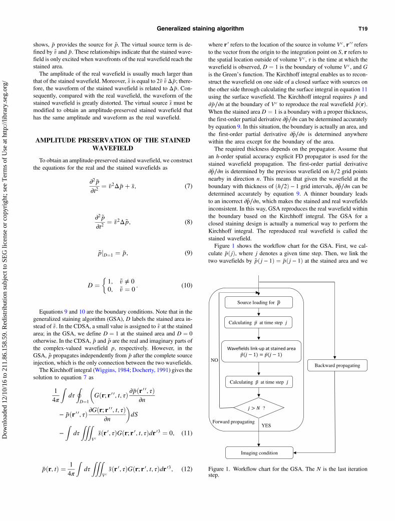
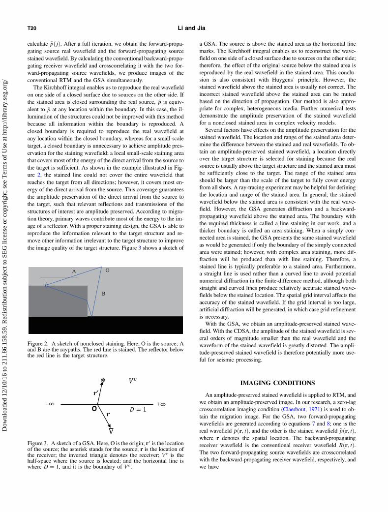
on one side of a closed surface due to sources on the other side. Ifthe stained area is closed surrounding the real source, ~p is equiv-alent to p̄ at any location within the boundary. In this case, the il-lumination of the structures could not be improved with this methodbecause all information within the boundary is reproduced. Aclosed boundary is required to reproduce the real wavefield atany location within the closed boundary, whereas for a small-scaletarget, a closed boundary is unnecessary to achieve amplitude pres-ervation for the staining wavefield; a local small-scale staining areathat covers most of the energy of the direct arrival from the source tothe target is sufficient. As shown in the example illustrated in Fig-ure 2, the stained line could not cover the entire wavefield thatreaches the target from all directions; however, it covers most en-ergy of the direct arrival from the source. This coverage guaranteesthe amplitude preservation of the direct arrival from the source tothe target, such that relevant reflections and transmissions of thestructures of interest are amplitude preserved. According to migra-tion theory, primary waves contribute most of the energy to the im-age of a reflector. With a proper staining design, the GSA is able toreproduce the information relevant to the target structure and re-move other information irrelevant to the target structure to improvethe image quality of the target structure. Figure 3 shows a sketch of

a GSA. The source is above the stained area as the horizontal linemarks. The Kirchhoff integral enables us to reconstruct the wave-field on one side of a closed surface due to sources on the other side;therefore, the effect of the original source below the stained area isreproduced by the real wavefield in the stained area. This conclu-sion is also consistent with Huygens’ principle. However, thestained wavefield above the stained area is usually not correct. Theincorrect stained wavefield above the stained area can be mutedbased on the direction of propagation. Our method is also appro-priate for complex, heterogeneous media. Further numerical testsdemonstrate the amplitude preservation of the stained wavefieldfor a nonclosed stained area in complex velocity models.Several factors have effects on the amplitude preservation for the

stained wavefield. The location and range of the stained area deter-mine the difference between the stained and real wavefields. To ob-tain an amplitude-preserved stained wavefield, a location directlyover the target structure is selected for staining because the realsource is usually above the target structure and the stained area mustbe sufficiently close to the target. The range of the stained areashould be larger than the scale of the target to fully cover energyfrom all shots. A ray-tracing experiment may be helpful for definingthe location and range of the stained area. In general, the stainedwavefield below the stained area is consistent with the real wave-field. However, the GSA generates diffraction and a backward-propagating wavefield above the stained area. The boundary withthe required thickness is called a line staining in our work, and athicker boundary is called an area staining. When a simply con-nected area is stained, the GSA presents the same stained wavefieldas would be generated if only the boundary of the simply connectedarea were stained; however, with complex area staining, more dif-fraction will be produced than with line staining. Therefore, astained line is typically preferable to a stained area. Furthermore,a straight line is used rather than a curved line to avoid potentialnumerical diffraction in the finite-difference method, although bothstraight and curved lines produce relatively accurate stained wave-fields below the stained location. The spatial grid interval affects theaccuracy of the stained wavefield. If the grid interval is too large,artificial diffraction will be generated, in which case grid refinementis necessary.With the GSA, we obtain an amplitude-preserved stained wave-

field. With the CDSA, the amplitude of the stained wavefield is sev-eral orders of magnitude smaller than the real wavefield and thewaveform of the stained wavefield is greatly distorted. The ampli-tude-preserved stained wavefield is therefore potentially more use-ful for seismic processing.

IMAGING CONDITIONS

An amplitude-preserved stained wavefield is applied to RTM, andwe obtain an amplitude-preserved image. In our research, a zero-lagcrosscorrelation imaging condition (Claerbout, 1971) is used to ob-tain the migration image. For the GSA, two forward-propagatingwavefields are generated according to equations 7 and 8; one is thereal wavefield p̄ðr; tÞ, and the other is the stained wavefield ~pðr; tÞ,where r denotes the spatial location. The backward-propagatingreceiver wavefield is the conventional receiver wavefield Rðr; tÞ.The two forward-propagating source wavefields are crosscorrelatedwith the backward-propagating receiver wavefield, respectively, andwe have

A

B

O

Figure 2. A sketch of nonclosed staining. Here, O is the source; Aand B are the raypaths. The red line is stained. The reflector belowthe red line is the target structure.

Figure 3. A sketch of a GSA. Here, O is the origin; r 0 is the locationof the source; the asterisk stands for the source; r is the location ofthe receiver; the inverted triangle denotes the receiver; Vc is thehalf-space where the source is located; and the horizontal line iswhere D ¼ 1, and it is the boundary of Vc.

T20 Li and Jia

Dow

nloa

ded

12/1

0/16

to 2

11.8

6.15

8.59

. Red

istr

ibut

ion

subj

ect t

o SE

G li

cens

e or

cop

yrig

ht; s

ee T

erm

s of

Use

at h

ttp://

libra

ry.s

eg.o

rg/

IrðrÞ ¼ZT

0

p̄ðr; tÞRðr; T − tÞdt; (13)

IsðrÞ ¼ZT

0

~pðr; tÞRðr; T − tÞdt; (14)

where T is the maximum recording time, IrðrÞ denotes the conven-tional RTM image, and IsðrÞ denotes the migration image generatedby the stained forward-propagating source wavefield. We call ~pðr; tÞthe generalized stained wavefield, and IsðrÞ the generalized stain-ing image.

NUMERICAL EXAMPLES

Several numerical experiments were con-ducted to demonstrate the application of the GSAin the modeling kernel of migration and RTM.The finite-difference method in the time–spacedomain is used in the following examples.A three-layered model is designed to evaluate

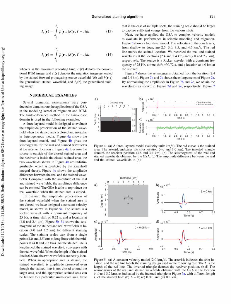
the amplitude preservation of the stained wave-field when the stained area is closed and irregularin heterogeneous media. Figure 4a shows thethree-layered model, and Figure 4b gives theseismograms for the real and stained wavefieldsat the receiver location in Figure 4a. Because thesource is outside of the closed stained area andthe receiver is inside the closed stained area, thetwo wavefields shown in Figure 4b are indistin-guishable, which is predicted by the Kirchhoffintegral theory. Figure 4c shows the amplitudedifference between the real and the stained wave-fields. Compared with the amplitude of the realand stained wavefields, the amplitude differencecan be omitted. The GSA is able to reproduce thereal wavefield when the stained area is closed.To evaluate the amplitude preservation of

the stained wavefield when the stained area isnot closed, we have designed a constant velocitymodel, as shown in Figure 5a. The source is aRicker wavelet with a dominant frequency of25 Hz, a time shift of 0.72 s, and a location at(4.0 and 2.4 km). Figure 5b–5d shows the seis-mograms of the stained and real wavefields at lo-cation (4.0 and 3.2 km) for different stainingscales. The staining scales vary from a singlepoint (4.0 and 2.5 km) to long lines with the mid-points at (4.0 and 2.5 km). As the stained line islengthened, the stained wavefield converges withthe real wavefield. When the length of the stainedline is 0.8 km, the twowavefields are nearly iden-tical. When an appropriate area is stained, thestained wavefield is amplitude preserved eventhough the stained line is not closed around thetarget area, and the appropriate stained area canbe limited to a particular small-scale area. Note

that in the case of multiple shots, the staining scale should be largerto capture sufficient energy from the various shots.Next, we have applied the GSA to complex velocity models

to evaluate its performance in seismic modeling and migration.Figure 6 shows a four-layer model. The velocities of the four layers,from shallow to deep, are 2.5, 3.0, 3.5, and 4.5 km∕s. The redline marks the stained location. We recorded the real and stainedwavefields at the locations (2.4 and 2.4 km) and (2.8 and 2.7 km),respectively. The source is a Ricker wavelet with a dominant fre-quency of 25 Hz, a time shift of 0.72 s, and a location at 4.0 km atthe surface.Figure 7 shows the seismograms obtained from the location (2.4

and 2.4 km). Figure 7b and 7c shows the enlargements of Figure 7a.By normalizing the amplitudes in Figure 7b and 7c, we obtain thewavefields as shown in Figure 7d and 7e, respectively. Figure 7

0.5 1 1.5 2 2.5 3 3.5 4 4.5 5 5.5 6−5

0

5 x 10−7

Time (s)A

mpl

itude

di

ffere

nce

0.5 1 1.5 2 2.5 3 3.5 4 4.5 5 5.5 6−5

0

5 x 10−3

Time (s)

Am

plitu

de Real wavefieldStained wavefield

0

1

2

3

4

5

6

Dep

th (

km)

0 1 2 3 4 5 6 7Distance (km)

2.0

2.5

3.0

3.5

4.0

*

a) b)

c)

Figure 4. (a) A three-layered model (velocity unit: km∕s). The red curve is the stainedarea. The asterisk indicates the shot location (4.0 and 1.6 km). The inverted triangledenotes the receiver position (3.6 and 3.4 km). (b) The seismograms of the real andstained wavefields obtained by the GSA. (c) The amplitude difference between the realand the stained wavefields in (b).

0

1

2

3

4

5

6

Dep

th (

km)

0 1 2 3 4 5 6 7Distance (km)

a)

0.4 0.5 0.6 0.7 0.8−5

0

5

10x 10

−3

L = 0 km

b)

Time (s)

Am

plitu

de

0.4 0.5 0.6 0.7 0.8−5

0

5

10x 10

−3

L = 0.08 km

c)

Time (s)

Am

plitu

de

0.4 0.5 0.6 0.7 0.8−5

0

5

10x 10

−3

L = 0.8 km

d)

Time (s)

Am

plitu

de

Figure 5. (a) A constant velocity model (2.0 km∕s). The asterisk indicates the shot lo-cation, and the red line labels the staining design used in the following test. The L is thelength of the red line. The inverted triangle denotes the receiver position. (b-d) Theseismograms of the real and stained wavefields obtained with the GSA at the location(4.0 and 3.2 km), as indicated by the inverted triangle in Figure 5a, with different lengthL of the stained line: (b) L ¼ 0; (c) 0.08; and (d) 0.8 km.

Generalized staining algorithm T21

Dow

nloa

ded

12/1

0/16

to 2

11.8

6.15

8.59

. Red

istr

ibut

ion

subj

ect t

o SE

G li

cens

e or

cop

yrig

ht; s

ee T

erm

s of

Use

at h

ttp://

libra

ry.s

eg.o

rg/

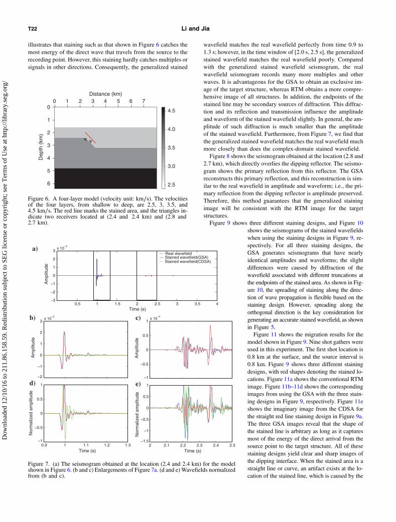
illustrates that staining such as that shown in Figure 6 catches themost energy of the direct wave that travels from the source to therecording point. However, this staining hardly catches multiples orsignals in other directions. Consequently, the generalized stained

wavefield matches the real wavefield perfectly from time 0.9 to1.3 s; however, in the time window of [2.0 s, 2.5 s], the generalizedstained wavefield matches the real wavefield poorly. Comparedwith the generalized stained wavefield seismogram, the realwavefield seismogram records many more multiples and otherwaves. It is advantageous for the GSA to obtain an exclusive im-age of the target structure, whereas RTM obtains a more compre-hensive image of all structures. In addition, the endpoints of thestained line may be secondary sources of diffraction. This diffrac-tion and its reflection and transmission influence the amplitudeand waveform of the stained wavefield slightly. In general, the am-plitude of such diffraction is much smaller than the amplitudeof the stained wavefield. Furthermore, from Figure 7, we find thatthe generalized stained wavefield matches the real wavefield muchmore closely than does the complex-domain stained wavefield.Figure 8 shows the seismogram obtained at the location (2.8 and

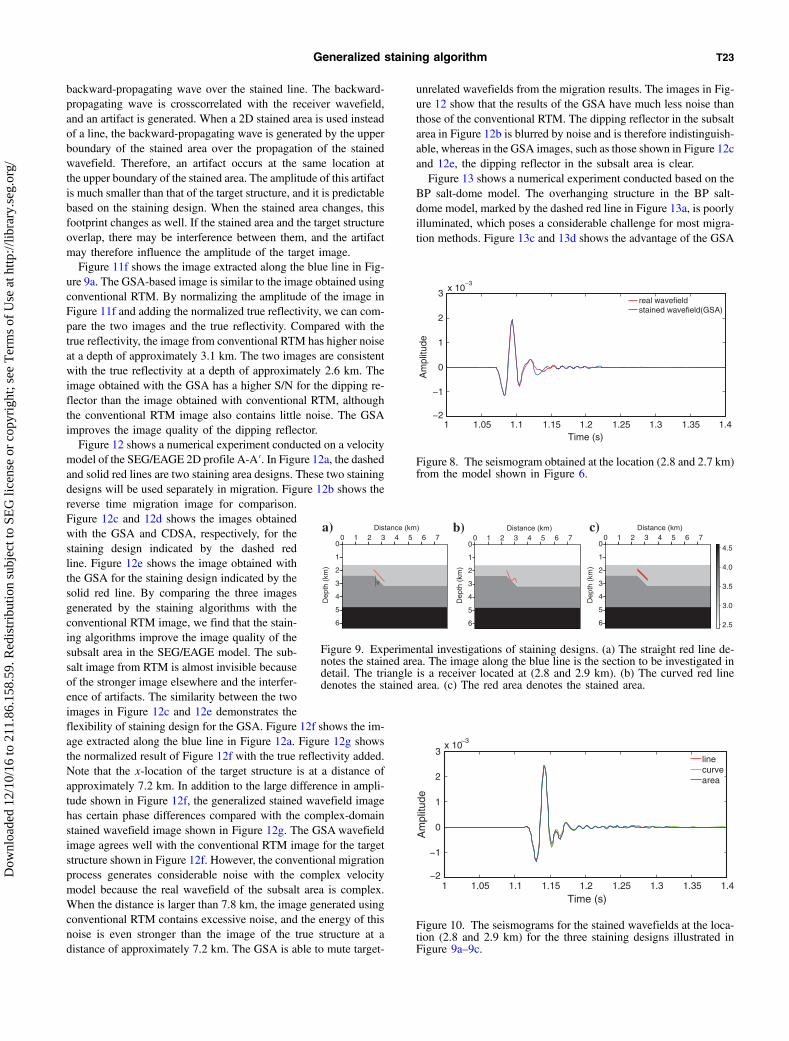
2.7 km), which directly overlies the dipping reflector. The seismo-gram shows the primary reflection from this reflector. The GSAreconstructs this primary reflection, and this reconstruction is sim-ilar to the real wavefield in amplitude and waveform; i.e., the pri-mary reflection from the dipping reflector is amplitude preserved.Therefore, this method guarantees that the generalized stainingimage will be consistent with the RTM image for the targetstructures.Figure 9 shows three different staining designs, and Figure 10

shows the seismograms of the stained wavefieldswhen using the staining designs in Figure 9, re-spectively. For all three staining designs, theGSA generates seismograms that have nearlyidentical amplitudes and waveforms; the slightdifferences were caused by diffraction of thewavefield associated with different truncations atthe endpoints of the stained area. As shown in Fig-ure 10, the spreading of staining along the direc-tion of wave propagation is flexible based on thestaining design. However, spreading along theorthogonal direction is the key consideration forgenerating an accurate stained wavefield, as shownin Figure 5.Figure 11 shows the migration results for the

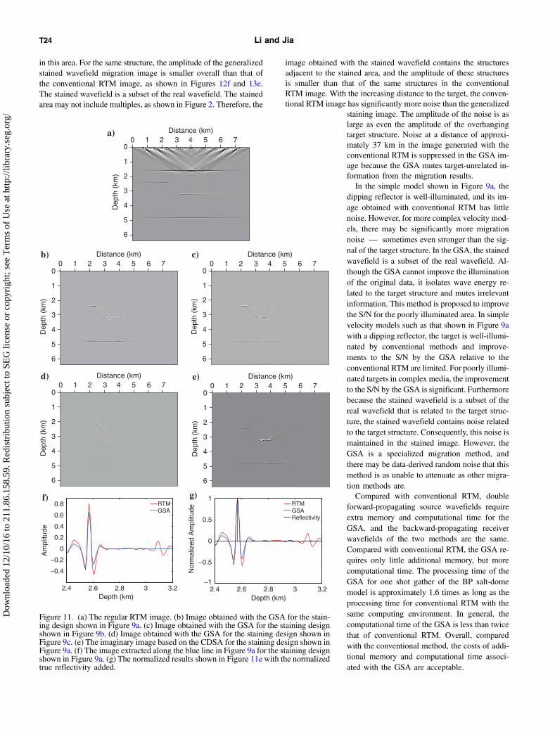
model shown in Figure 9. Nine shot gathers wereused in this experiment. The first shot location is0.8 km at the surface, and the source interval is0.8 km. Figure 9 shows three different stainingdesigns, with red shapes denoting the stained lo-cations. Figure 11a shows the conventional RTMimage. Figure 11b–11d shows the correspondingimages from using the GSAwith the three stain-ing designs in Figure 9, respectively. Figure 11eshows the imaginary image from the CDSA forthe straight red line staining design in Figure 9a.The three GSA images reveal that the shape ofthe stained line is arbitrary as long as it capturesmost of the energy of the direct arrival from thesource point to the target structure. All of thesestaining designs yield clear and sharp images ofthe dipping interface. When the stained area is astraight line or curve, an artifact exists at the lo-cation of the stained line, which is caused by the

0

1

2

3

4

5

6

Dep

th (

km)

0 1 2 3 4 5 6 7Distance (km)

2.5

3.0

3.5

4.0

4.5

Figure 6. A four-layer model (velocity unit: km∕s). The velocitiesof the four layers, from shallow to deep, are 2.5, 3, 3.5, and4.5 km∕s. The red line marks the stained area, and the triangles in-dicate two receivers located at (2.4 and 2.4 km) and (2.8 and2.7 km).

−2

−1

0

1

2

3x 10

−3

x 10−3

Am

plitu

de

0.9 1 1.1 1.2 1.3−1

−0.5

0

0.5

1

Time (s)

Nor

mal

ized

am

plitu

de

−1

−0.5

0

0.5

1x 10

−4

Am

plitu

de

2 2.1 2.2 2.3 2.4 2.5−1.5

−1

−0.5

0

0.5

1

Time (s)

Nor

mal

ized

am

plitu

de

b) c)

d) e)

0.5 1 1.5 2 2.5 3 3.5 4−3

−2

−1

0

1

2

3

Time (s)

Am

plitu

de

Real wavefieldStained wavefield(GSA)Stained wavefield(CDSA)

a)

Figure 7. (a) The seismogram obtained at the location (2.4 and 2.4 km) for the modelshown in Figure 6. (b and c) Enlargements of Figure 7a. (d and e) Wavefields normalizedfrom (b and c).

T22 Li and Jia

Dow

nloa

ded

12/1

0/16

to 2

11.8

6.15

8.59

. Red

istr

ibut

ion

subj

ect t

o SE

G li

cens

e or

cop

yrig

ht; s

ee T

erm

s of

Use

at h

ttp://

libra

ry.s

eg.o

rg/

backward-propagating wave over the stained line. The backward-propagating wave is crosscorrelated with the receiver wavefield,and an artifact is generated. When a 2D stained area is used insteadof a line, the backward-propagating wave is generated by the upperboundary of the stained area over the propagation of the stainedwavefield. Therefore, an artifact occurs at the same location atthe upper boundary of the stained area. The amplitude of this artifactis much smaller than that of the target structure, and it is predictablebased on the staining design. When the stained area changes, thisfootprint changes as well. If the stained area and the target structureoverlap, there may be interference between them, and the artifactmay therefore influence the amplitude of the target image.Figure 11f shows the image extracted along the blue line in Fig-

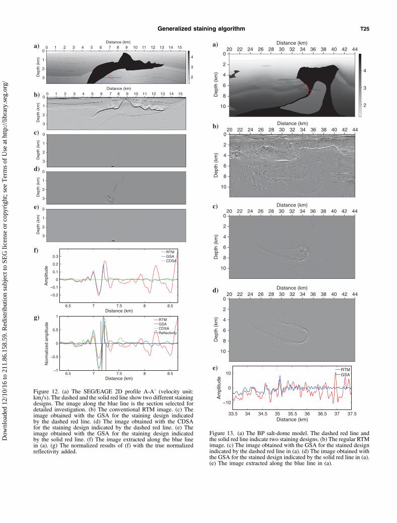
ure 9a. The GSA-based image is similar to the image obtained usingconventional RTM. By normalizing the amplitude of the image inFigure 11f and adding the normalized true reflectivity, we can com-pare the two images and the true reflectivity. Compared with thetrue reflectivity, the image from conventional RTM has higher noiseat a depth of approximately 3.1 km. The two images are consistentwith the true reflectivity at a depth of approximately 2.6 km. Theimage obtained with the GSA has a higher S/N for the dipping re-flector than the image obtained with conventional RTM, althoughthe conventional RTM image also contains little noise. The GSAimproves the image quality of the dipping reflector.Figure 12 shows a numerical experiment conducted on a velocity

model of the SEG/EAGE 2D profile A-A′. In Figure 12a, the dashedand solid red lines are two staining area designs. These two stainingdesigns will be used separately in migration. Figure 12b shows thereverse time migration image for comparison.Figure 12c and 12d shows the images obtainedwith the GSA and CDSA, respectively, for thestaining design indicated by the dashed redline. Figure 12e shows the image obtained withthe GSA for the staining design indicated by thesolid red line. By comparing the three imagesgenerated by the staining algorithms with theconventional RTM image, we find that the stain-ing algorithms improve the image quality of thesubsalt area in the SEG/EAGE model. The sub-salt image from RTM is almost invisible becauseof the stronger image elsewhere and the interfer-ence of artifacts. The similarity between the twoimages in Figure 12c and 12e demonstrates theflexibility of staining design for the GSA. Figure 12f shows the im-age extracted along the blue line in Figure 12a. Figure 12g showsthe normalized result of Figure 12f with the true reflectivity added.Note that the x-location of the target structure is at a distance ofapproximately 7.2 km. In addition to the large difference in ampli-tude shown in Figure 12f, the generalized stained wavefield imagehas certain phase differences compared with the complex-domainstained wavefield image shown in Figure 12g. The GSA wavefieldimage agrees well with the conventional RTM image for the targetstructure shown in Figure 12f. However, the conventional migrationprocess generates considerable noise with the complex velocitymodel because the real wavefield of the subsalt area is complex.When the distance is larger than 7.8 km, the image generated usingconventional RTM contains excessive noise, and the energy of thisnoise is even stronger than the image of the true structure at adistance of approximately 7.2 km. The GSA is able to mute target-

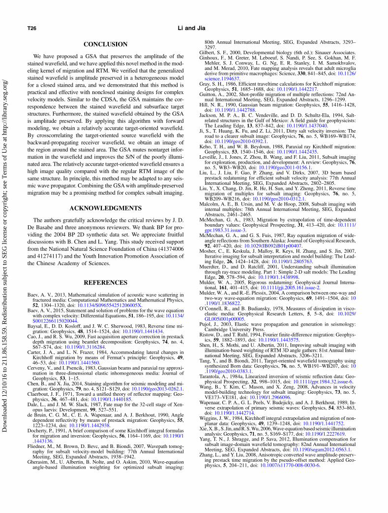
unrelated wavefields from the migration results. The images in Fig-ure 12 show that the results of the GSA have much less noise thanthose of the conventional RTM. The dipping reflector in the subsaltarea in Figure 12b is blurred by noise and is therefore indistinguish-able, whereas in the GSA images, such as those shown in Figure 12cand 12e, the dipping reflector in the subsalt area is clear.Figure 13 shows a numerical experiment conducted based on the

BP salt-dome model. The overhanging structure in the BP salt-dome model, marked by the dashed red line in Figure 13a, is poorlyilluminated, which poses a considerable challenge for most migra-tion methods. Figure 13c and 13d shows the advantage of the GSA

1 1.05 1.1 1.15 1.2 1.25 1.3 1.35 1.4−2

−1

0

1

2

3 x 10−3

Time (s)

Am

plitu

de

real wavefieldstained wavefield(GSA)

Figure 8. The seismogram obtained at the location (2.8 and 2.7 km)from the model shown in Figure 6.

0

1

2

3

4

5

6

Dep

th (k

m)

0 1 2 3 4 5 6 7Distance (km)

0

1

2

3

4

5

6

Dep

th (k

m)

0 1 2 3 4 5 6 7Distance (km)

0

1

2

3

4

5

6

Dep

th (k

m)

0 1 2 3 4 5 6 7Distance (km)

2.5

3.0

3.5

4.0

4.5

c)b)a)

▽

Figure 9. Experimental investigations of staining designs. (a) The straight red line de-notes the stained area. The image along the blue line is the section to be investigated indetail. The triangle is a receiver located at (2.8 and 2.9 km). (b) The curved red linedenotes the stained area. (c) The red area denotes the stained area.

1 1.05 1.1 1.15 1.2 1.25 1.3 1.35 1.4−2

−1

0

1

2

3x 10

−3

Time (s)

Am

plitu

de

linecurvearea

Figure 10. The seismograms for the stained wavefields at the loca-tion (2.8 and 2.9 km) for the three staining designs illustrated inFigure 9a–9c.

Generalized staining algorithm T23

Dow

nloa

ded

12/1

0/16

to 2

11.8

6.15

8.59

. Red

istr

ibut

ion

subj

ect t

o SE

G li

cens

e or

cop

yrig

ht; s

ee T

erm

s of

Use

at h

ttp://

libra

ry.s

eg.o

rg/

in this area. For the same structure, the amplitude of the generalizedstained wavefield migration image is smaller overall than that ofthe conventional RTM image, as shown in Figures 12f and 13e.The stained wavefield is a subset of the real wavefield. The stainedarea may not include multiples, as shown in Figure 2. Therefore, the

image obtained with the stained wavefield contains the structuresadjacent to the stained area, and the amplitude of these structuresis smaller than that of the same structures in the conventionalRTM image. With the increasing distance to the target, the conven-tional RTM image has significantly more noise than the generalized

staining image. The amplitude of the noise is aslarge as even the amplitude of the overhangingtarget structure. Noise at a distance of approxi-mately 37 km in the image generated with theconventional RTM is suppressed in the GSA im-age because the GSA mutes target-unrelated in-formation from the migration results.In the simple model shown in Figure 9a, the

dipping reflector is well-illuminated, and its im-age obtained with conventional RTM has littlenoise. However, for more complex velocity mod-els, there may be significantly more migrationnoise — sometimes even stronger than the sig-nal of the target structure. In the GSA, the stainedwavefield is a subset of the real wavefield. Al-though the GSA cannot improve the illuminationof the original data, it isolates wave energy re-lated to the target structure and mutes irrelevantinformation. This method is proposed to improvethe S/N for the poorly illuminated area. In simplevelocity models such as that shown in Figure 9awith a dipping reflector, the target is well-illumi-nated by conventional methods and improve-ments to the S/N by the GSA relative to theconventional RTM are limited. For poorly illumi-nated targets in complex media, the improvementto the S/N by the GSA is significant. Furthermorebecause the stained wavefield is a subset of thereal wavefield that is related to the target struc-ture, the stained wavefield contains noise relatedto the target structure. Consequently, this noise ismaintained in the stained image. However, theGSA is a specialized migration method, andthere may be data-derived random noise that thismethod is as unable to attenuate as other migra-tion methods are.Compared with conventional RTM, double

forward-propagating source wavefields requireextra memory and computational time for theGSA, and the backward-propagating receiverwavefields of the two methods are the same.Compared with conventional RTM, the GSA re-quires only little additional memory, but morecomputational time. The processing time of theGSA for one shot gather of the BP salt-domemodel is approximately 1.6 times as long as theprocessing time for conventional RTM with thesame computing environment. In general, thecomputational time of the GSA is less than twicethat of conventional RTM. Overall, comparedwith the conventional method, the costs of addi-tional memory and computational time associ-ated with the GSA are acceptable.

0

1

2

3

4

5

6

Dep

th (

km)

b)

0

1

2

3

4

5

6

Dep

th (

km)

c)

0

1

2

3

4

5

6

Dep

th (

km)

d)

0

1

2

3

4

5

6

Dep

th (

km)

e)

0

1

2

3

4

5

6

Dep

th (

km)

0 1 2 3 4 5 6 7Distance (km)

0 1 2 3 4 5 6 7Distance (km)

0 1 2 3 4 5 6 7Distance (km)

0 1 2 3 4 5 6 7Distance (km)

0 1 2 3 4 5 6 7Distance (km)

2.4 2.6 2.8 3 3.2

−0.4

−0.2

0

0.2

0.4

0.6

0.8

Depth (km)

Am

plitu

de

RTMGSA

2.4 2.6 2.8 3 3.2−1

−0.5

0

0.5

1

Depth (km)

Nor

mal

ized

Am

plitu

de

RTMGSAReflectivity

f) g)

a)

Figure 11. (a) The regular RTM image. (b) Image obtained with the GSA for the stain-ing design shown in Figure 9a. (c) Image obtained with the GSA for the staining designshown in Figure 9b. (d) Image obtained with the GSA for the staining design shown inFigure 9c. (e) The imaginary image based on the CDSA for the staining design shown inFigure 9a. (f) The image extracted along the blue line in Figure 9a for the staining designshown in Figure 9a. (g) The normalized results shown in Figure 11e with the normalizedtrue reflectivity added.

T24 Li and Jia

Dow

nloa

ded

12/1

0/16

to 2

11.8

6.15

8.59

. Red

istr

ibut

ion

subj

ect t

o SE

G li

cens

e or

cop

yrig

ht; s

ee T

erm

s of

Use

at h

ttp://

libra

ry.s

eg.o

rg/

0

1

2

3

Dep

th (

km)

0

1

2

3

Dep

th (

km)

0

1

2

3

Dep

th (

km)

c)

d)

e)

0

1

2

3

Dep

th (

km)

b)

0

1

2

3Dep

th (

km)

0 1 2 3 4 5 6 7 8 9 10 11 12 13 14 15Distance (km)

0 1 2 3 4 5 6 7 8 9 10 11 12 13 14 15Distance (km)

2

3

4

a)

6.5 7 7.5 8 8.5

−0.2

−0.1

0

0.1

0.2

0.3

Distance (km)

Am

plitu

de

RTMGSACDSA

f)

6.5 7 7.5 8 8.5−1

−0.5

0

0.5

1

Distance (km)

Nor

mal

ized

am

plitu

de

RTMGSACDSAReflectivity

g)

Figure 12. (a) The SEG/EAGE 2D profile A-A′ (velocity unit:km∕s). The dashed and the solid red line show two different stainingdesigns. The image along the blue line is the section selected fordetailed investigation. (b) The conventional RTM image. (c) Theimage obtained with the GSA for the staining design indicatedby the dashed red line. (d) The image obtained with the CDSAfor the staining design indicated by the dashed red line. (e) Theimage obtained with the GSA for the staining design indicatedby the solid red line. (f) The image extracted along the blue linein (a). (g) The normalized results of (f) with the true normalizedreflectivity added.

0

2

4

6

8

10

Dep

th (

km)

20 22 24 26 28 30 32 34 36 38 40 42 44Distance (km)

2

3

4

0

2

4

6

8

10

Dep

th (

km)

20 22 24 26 28 30 32 34 36 38 40 42 44Distance (km)

0

2

4

6

8

10

Dep

th (

km)

20 22 24 26 28 30 32 34 36 38 40 42 44Distance (km)

0

2

4

6

8

10

Dep

th (

km)

20 22 24 26 28 30 32 34 36 38 40 42 44Distance (km)c)

d)

b)

a)

33.5 34 34.5 35 35.5 36 36.5 37 37.5

−10

0

10

Distance (km)

Am

plitu

de

RTMGSA

e)

Figure 13. (a) The BP salt-dome model. The dashed red line andthe solid red line indicate two staining designs. (b) The regular RTMimage. (c) The image obtained with the GSA for the stained designindicated by the dashed red line in (a). (d) The image obtained withthe GSA for the stained design indicated by the solid red line in (a).(e) The image extracted along the blue line in (a).

Generalized staining algorithm T25

Dow

nloa

ded

12/1

0/16

to 2

11.8

6.15

8.59

. Red

istr

ibut

ion

subj

ect t

o SE

G li

cens

e or

cop

yrig

ht; s

ee T

erm

s of

Use

at h

ttp://

libra

ry.s

eg.o

rg/

CONCLUSION

We have proposed a GSA that preserves the amplitude of thestained wavefield, and we have applied this novel method in the mod-eling kernel of migration and RTM. We verified that the generalizedstained wavefield is amplitude preserved in a heterogeneous modelfor a closed stained area, and we demonstrated that this method ispractical and effective with nonclosed staining designs for complexvelocity models. Similar to the CDSA, the GSA maintains the cor-respondence between the stained wavefield and subsurface targetstructures. Furthermore, the stained wavefield obtained by the GSAis amplitude preserved. By applying this algorithm with forwardmodeling, we obtain a relatively accurate target-oriented wavefield.By crosscorrelating the target-oriented source wavefield with thebackward-propagating receiver wavefield, we obtain an image ofthe region around the stained area. The GSA mutes nontarget infor-mation in the wavefield and improves the S/N of the poorly illumi-nated area. The relatively accurate target-oriented wavefield ensures ahigh image quality compared with the regular RTM image of thesame structure. In principle, this method may be adapted to any seis-mic wave propagator. Combining the GSAwith amplitude-preservedmigration may be a promising method for complex subsalt imaging.

ACKNOWLEDGMENTS

The authors gratefully acknowledge the critical reviews by J. D.De Basabe and three anonymous reviewers. We thank BP for pro-viding the 2004 BP 2D synthetic data set. We appreciate fruitfuldiscussions with B. Chen and L. Yang. This study received supportfrom the National Natural Science Foundation of China (41374006and 41274117) and the Youth Innovation Promotion Association ofthe Chinese Academy of Sciences.

REFERENCES

Baev, A. V., 2013, Mathematical simulation of acoustic wave scattering infractured media: Computational Mathematics and Mathematical Physics,52, 1304–1320, doi: 10.1134/S096554251206005X.

Baev, A. V., 2015, Statement and solution of problems for the wave equationwith complex velocity: Differential Equations, 51, 186–195, doi: 10.1134/S0012266115020044.

Baysal, E., D. D. Kosloff, and J. W. C. Sherwood, 1983, Reverse time mi-gration: Geophysics, 48, 1514–1524, doi: 10.1190/1.1441434.

Cao, J., and R. S. Wu, 2009, Fast acquisition aperture correction in prestackdepth migration using beamlet decomposition: Geophysics, 74, no. 4,S67–S74, doi: 10.1190/1.3116284.

Carter, J. A., and L. N. Frazer, 1984, Accommodating lateral changes inKirchhoff migration by means of Fermat’s principle: Geophysics, 49,46–53, doi: 10.1190/1.1441560.

Cerveny, V., and I. Psencik, 1983, Gaussian beams and paraxial ray approxi-mation in three-dimensional elastic inhomogeneous media: Journal ofGeophysics, 53, 1–15.

Chen, B., and X. Jia, 2014, Staining algorithm for seismic modeling and mi-gration: Geophysics, 79, no. 4, S121–S129, doi: 10.1190/geo2013-0262.1.

Claerbout, J. F., 1971, Toward a unified theory of reflector mapping: Geo-physics, 36, 467–481, doi: 10.1190/1.1440185.

Dale, L., and J. M. W. Slack, 1987, Fate map for the 32-cell stage of Xen-opus laevis: Development, 99, 527–551.

de Bruin, C. G. M., C. E. A. Wapenaar, and A. J. Berkhout, 1990, Angledependent reflectivity by means of prestack migration: Geophysics, 55,1223–1234, doi: 10.1190/1.1442938.

Docherty, P., 1991, A brief comparison of some Kirchhoff integral formulasfor migration and inversion: Geophysics, 56, 1164–1169, doi: 10.1190/1.1443136.

Fliedner, M., M. Brown, D. Bevc, and B. Biondi, 2007, Wavepath tomog-raphy for subsalt velocity-model building: 77th Annual InternationalMeeting, SEG, Expanded Abstracts, 1938–1942.

Gherasim, M., U. Albertin, B. Nolte, and O. Askim, 2010, Wave-equationangle-based illumination weighting for optimized subsalt imaging:

80th Annual International Meeting, SEG, Expanded Abstracts, 3293–3297.

Gilbert, S. F., 2000, Developmental biology (6th ed.): Sinauer Associates.Ginhoux, F., M. Greter, M. Leboeuf, S. Nandi, P. See, S. Gokhan, M. F.

Mehler, S. J. Conway, L. G. Ng, E. R. Stanley, I. M. Samokhvalov,and M. Merad, 2010, Fate mapping analysis reveals that adult microgliaderive from primitive macrophages: Science, 330, 841–845, doi: 10.1126/science.1194637.

Gray, S. H., 1986, Efficient traveltime calculations for Kirchhoff migration:Geophysics, 51, 1685–1688, doi: 10.1190/1.1442217.

Guitton, A., 2002, Shot-profile migration of multiple reflections: 72nd An-nual International Meeting, SEG, Expanded Abstracts, 1296–1299.

Hill, N. R., 1990, Gaussian beam migration: Geophysics, 55, 1416–1428,doi: 10.1190/1.1442788.

Jackson, M. P. A., B. C. Vendeville, and D. D. Schultz-Ela, 1994, Salt-related structures in the Gulf of Mexico: A field guide for geophysicists:The Leading Edge, 13, 837–842, doi: 10.1190/1.1437040.

Ji, S., T. Huang, K. Fu, and Z. Li, 2011, Dirty salt velocity inversion: Theroad to a clearer subsalt image: Geophysics, 76, no. 5, WB169–WB174,doi: 10.1190/geo2010-0392.1.

Keho, T. H., and W. B. Beydoun, 1988, Paraxial ray Kirchhoff migration:Geophysics, 53, 1540–1546, doi: 10.1190/1.1442435.

Leveille, J., I. Jones, Z. Zhou, B. Wang, and F. Liu, 2011, Subsalt imagingfor exploration, production, and development: A review: Geophysics, 76,no. 5, WB3–WB20, doi: 10.1190/geo2011-0156.1.

Liu, L., J. Liu, F. Gao, P. Zhang, and V. Dirks, 2007, 3D beam basedprestack redatuming for efficient subsalt velocity analysis: 77th AnnualInternational Meeting, SEG, Expanded Abstracts, 2802–2805.

Liu, Y., X. Chang, D. Jin, R. He, H. Sun, and Y. Zheng, 2011, Reverse timemigration of multiples for subsalt imaging: Geophysics, 76, no. 5,WB209–WB216, doi: 10.1190/geo2010-0312.1.

Malcolm, A. E., B. Ursin, and M. V. de Hoop, 2008, Subsalt imaging withinternal multiples: 78th Annual International Meeting, SEG, ExpandedAbstracts, 2461–2465.

McMechan, G. A., 1983, Migration by extrapolation of time-dependentboundary values: Geophysical Prospecting, 31, 413–420, doi: 10.1111/gpr.1983.31.issue-3.

McMechan, G. A., and G. S. Fuis, 1987, Ray equation migration of wide-angle reflections from Southern Alaska: Journal of Geophysical Research,92, 407–420, doi: 10.1029/JB092iB01p00407.

Mosher, C., E. Keskula, J. Malloy, R. Keys, H. Zhang, and S. Jin, 2007,Iterative imaging for subsalt interpretation and model building: The Lead-ing Edge, 26, 1424–1428, doi: 10.1190/1.2805763.

Muerdter, D., and D. Ratcliff, 2001, Understanding subsalt illuminationthrough ray-trace modeling. Part 1: Simple 2-D salt models: The LeadingEdge, 20, 578–594, doi: 10.1190/1.1438998.

Mulder, W. A., 2005, Rigorous redatuming: Geophysical Journal Interna-tional, 161, 401–415, doi: 10.1111/gji.2005.161.issue-2.

Mulder, W. A., and R.-E. Plessix, 2004, A comparison between one-way andtwo-way wave-equation migration: Geophysics, 69, 1491–1504, doi: 10.1190/1.1836822.

O’Connell, R., and B. Budiansky, 1978, Measures of dissipation in visco-elastic media: Geophysical Research Letters, 5, 5–8, doi: 10.1029/GL005i001p00005.

Pujol, J., 2003, Elastic wave propagation and generation in seismology:Cambridge University Press.

Ristow, D., and T. Ruhl, 1994, Fourier finite-difference migration: Geophys-ics, 59, 1882–1893, doi: 10.1190/1.1443575.

Shen, H., S. Mothi, and U. Albertin, 2011, Improving subsalt imaging withillumination-based weighting of RTM 3D angle gathers: 81st Annual Inter-national Meeting, SEG, Expanded Abstracts, 3206–3211.

Tang, Y., and B. Biondi, 2011, Target-oriented wavefield tomography usingsynthesized Born data: Geophysics, 76, no. 5, WB191–WB207, doi: 10.1190/geo2010-0383.1.

Tarantola, A., 1984a, Linearized inversion of seismic reflection data: Geo-physical Prospecting, 32, 998–1015, doi: 10.1111/gpr.1984.32.issue-6.

Wang, B., Y. Kim, C. Mason, and X. Zeng, 2008, Advances in velocitymodel-building technology for subsalt imaging: Geophysics, 73, no. 5,VE173–VE181, doi: 10.1190/1.2966096.

Wapenaar, C. P. A., G. L. Peels, V. Budejicky, and A. J. Berkhout, 1989, In-verse extrapolation of primary seismic waves: Geophysics, 54, 853–863,doi: 10.1190/1.1442714.

Wiggins, J. W., 1984, Kirchhoff integral extrapolation and migration of non-planar data: Geophysics, 49, 1239–1248, doi: 10.1190/1.1441752.

Xie,X.B.,S.Jin, andR.S.Wu,2006,Wave-equationbasedseismic illuminationanalysis: Geophysics, 71, no. 5, S169–S177, doi: 10.1190/1.2227619.

Yang, T. N., J. Shragge, and P. Sava, 2012, Illumination compensation forsubsalt image-domain wavefield tomography: 82nd Annual InternationalMeeting, SEG, Expanded Abstracts, doi: 10.1190/segam2012-0563.1.

Zhang, L., and Y. Liu, 2008, Anisotropic converted wave amplitude-preserv-ing prestack time migration by the pseudo-offset method: Applied Geo-physics, 5, 204–211, doi: 10.1007/s11770-008-0030-6.

T26 Li and Jia

Dow

nloa

ded

12/1

0/16

to 2

11.8

6.15

8.59

. Red

istr

ibut

ion

subj

ect t

o SE

G li

cens

e or

cop

yrig

ht; s

ee T

erm

s of

Use

at h

ttp://

libra

ry.s

eg.o

rg/