generalizing experimental results by leveraging knowledge
TRANSCRIPT

Generalizing Experimental Results byLeveraging Knowledge of Mechanisms
Carlos Cinelli and Judea Pearl∗
University of California, Los AngelesDepartments of Statistics and Computer Science
[email protected], [email protected]
Abstract
We show how experimental results can be generalized across di-verse populations by leveraging knowledge of local mechanisms thatproduce the outcome of interest, only some of which may differ inthe target domain. We use Structural Causal Models (SCM) and arefined version of selection diagrams to represent such knowledge, andto decide whether it entails the invariance of probabilities of causationacross populations, which then enables generalization. We furtherprovide: (i) bounds for the target effect when some of these condi-tions are violated; (ii) new identification results for probabilities ofcausation and the transported causal effect when trials from multi-ple source domains are available; as well as (iii) a Bayesian approachfor estimating the transported causal effect from finite samples. Weillustrate these methods both with simulated data and with a real ex-ample that transports the effects of Vitamin A supplementation onchildhood mortality across different regions.
∗We thank Anders Huitfeldt, Ricardo Silva, and anonymous reviewers for valuablecomments and feedback. This research was supported in parts by grants from DefenseAdvanced Research Projects Agency [#W911NF-16-057], National Science Foundation[#IIS-1302448, #IIS-1527490, and #IIS-1704932], and Office of Naval Research [#N00014-17-S-B001].
1
Accepted to European Journal of Epidemiology. TECHNICAL REPORT R-492
September 2020
1 Introduction
Generalizing results of randomized control trials (RCT) is critical in manyempirical sciences and demands an understanding of the conditions underwhich such generalizations are feasible. When the mechanisms that de-termine the outcome differ between the study population and the targetpopulation, generalization requires measuring the variables responsible forsuch differences or, if this is not possible, isolating them away by measuringother variables (Pearl and Bareinboim, 2014). Recent work (Huitfeldt et al.,2018, 2019; Huitfeldt, 2019) describes an interesting situation under whichtransportability across populations is feasible without such measurements.This feasibility, however, is not immediately inferable using a standard (non-parametric) selection diagram (Pearl and Bareinboim, 2014; Bareinboim andPearl, 2016), because it relies on the invariance of only some components ofthe outcome mechanism, but not all.
In this paper, we use the theory of Structural Causal Models (SCM)(Pearl, 2009) to show how generalization in these settings can be modeledusing ordinary structural equations, counterfactual logic and selection dia-grams. We demonstrate that it requires two key assumptions: (i) the in-dependence of causal factors that affect the outcome; and, (ii) functionalconstraints on how these factors interact to produce the outcome. The com-bination of these assumptions may entail the invariance of certain probabil-ities of causation (Pearl, 1999; Tian and Pearl, 2000) across domains, thusallowing the transport of causal effects in settings where non-parametric gen-eralization is otherwise impossible.
We further extend the results of existing literature by: (i) relaxing themonotonicity assumption and providing bounds for the causal effect in thetarget domain; (ii) deriving novel identification and over-identification re-sults for probabilities of causation, as well as the transported causal effect,when trials from multiple source domains are available; and, (iii) providinga Bayesian framework for estimating the transported causal effect from fi-nite samples. We illustrate these methods both in simulated data and in areal example that generalizes the effects of Vitamin A supplementation onchildhood mortality across different regions (Sommer et al., 1986; Muhilalet al., 1988; West Jr et al., 1991). Open source software for R implementsthe methods discussed in this paper.1
1Available in https://github.com/carloscinelli/generalizing.
2
2 Motivating example
To fix ideas, we borrow the “Russian Roulette” example from Huitfeldt(2019). Although stylized, this intuitive example illustrates the key featuresof the problem.
A Russian Roulette trial
Suppose the city of Los Angeles decides to run a randomized control trial(RCT) to assess the effect of playing “Russian Roulette” on mortality.2 Afterrunning the experiment, the mayor of Los Angeles discovers that “RussianRoulette” is harmful: among those assigned to play Russian Roulette, 17.5%of the people died, as compared to only 1% among those who were notassigned to play the game (people can die due to other causes during thetrial, for example, prior poor health conditions).
After hearing the news about the Los Angeles experiment, the mayor ofNew York City (a dictator) wonders what the overall mortality rate would beif the city forced everyone to play Russian Roulette. Currently, the practiceof Russian Roulette is forbidden in New York, and its mortality rate is at 5%(4% higher than LA). The mayor thus asks the city’s statistician to decidewhether and how one could use the data from from Los Angeles to predictthe mortality rate in New York, once the new policy is implemented.
Intuitively, our causal knowledge of the domain permits us to answerthe question posed by the NYC mayor. Mortality is a consequence of two“independent” processes (the game of Russian Roulette and prior health con-ditions of the individual), and while the first factor remains unaltered acrosscities, the second intensifies by a known amount (5% vs 1%). Moreover, wecan safely assume that the two processes interact disjunctively, namely, thatdeath occurs if and only if at least one of the two processes takes effect. Fromthese two assumptions and elementary probability theory, we can concludethat mortality in NYC would be 20.8%. In section 3 we will cast this intu-ition into a formal setting, define this notion of “independence,” and showhow the data from NYC and LA should be combined to match our expec-tation. But before that, let us examine how this intuition clashes with theconclusion of a coarse analysis using selection diagrams.
2Russian Roulette consists of loading a bullet into a revolver, spinning the cylinder,pointing the gun at one’s own head and then pulling the trigger. We do not recommendattempting this.
3
An “impossibility” result
Selection diagrams are causal diagrams enriched with “selection nodes” S,usually represented by square nodes (�). These new nodes are used by theanalyst to indicate which local mechanisms are suspected to differ betweentwo environments (in our example, the mortality mechanism is suspected todiffer between Los Angeles and New York). More importantly, the absenceof a selection node pointing to a variable represents the assumption that thelocal mechanism responsible for assigning the value to that variable is thesame in the two populations (Pearl, 1995, 2009; Pearl and Bareinboim, 2014;Bareinboim and Pearl, 2016).
To build our selection diagram, we need to introduce some notation. Thepopulation of Los Angeles will be denoted by Π (the “source population”) andthat of New York by Π∗ (the “target population”). The random variable Ystands for mortality, with events Y = 1 denoting “death” and Y = 0 denoting“survival;” the random variable X stands for the “treatment” assignment,with events X = 1 denoting “play Russian Roulette” and X = 0 denoting“not play Russian Roulette.” The random variable Yx denotes the potentialresponse of Y when the treatment X is experimentally set to x. Thus,mathematically, the findings of the RCT can be translated to P (Y1 = 1) =17.5% and P (Y0 = 1) = 1%, and the available data from New York is P ∗(Y0 =1) = 5%. Our task is to estimate P ∗(Y1 = 1).
YX
(a) Coarse causal diagram
YX
S
(b) Coarse selection diagram
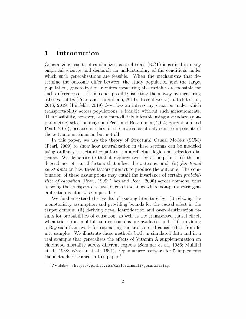
Figure 1: Coarse causal (a) and selection (b) diagrams of the RussianRoulette trial. The presence of S → Y in (b) correctly prohibits the naivetransportation of the interventional distribution P (Yx) from the source Π(Los Angeles) to the target environment Π∗ (New York).
The coarsest causal diagram of the Russian Roulette trial comprises onlythe treatment X and the outcome Y , as shown in Figure 1a. To move fromthe causal diagram to the selection diagram, we need to think of what maydiffer between LA and NYC. Since we already know from the data that
4
P (Y0 = 1) 6= P ∗(Y0 = 1), we suspect there are differences in the way mor-tality is determined in the two cities (for example, people in New York maybe in poorer health conditions, or the air quality may be worse). Thus, theselection diagram must contain a selection node S pointing to the mortalityvariable Y to indicate this disparity, as shown in Figure 1b.
Graphically, checking whether a causal relationship is transportable fromone environment to another involves checking whether there exists a set ofmeasurements that d-separates (Pearl, 2009) the source of disparity (the se-lection node S) from our target quantity. The presence of the selection nodepointing directly into Y prevents the separation of S from Y , and leads usto conclude that transportability is impossible without further assumptions.On the other hand, the intuition that led us to predict the new mortality ratein NYC tells us that such assumptions, once formalized, could license trans-portability. This intuition, as we discussed, was based on two assumptionsthat are not shown in the coarse selection diagram of Figure 1. The diagramrepresents only the existence of a disparity between LA and NYC, not thefact that it is localized to one cause of death (prior health factors), and thatit does not extend to the other cause (the game of Russian Roulette). As aresult, the diagram correctly warns us that, absent further assumptions, weare not authorized to make any generalization between the two cities.
3 Building the structural model
We now explicate formally what we know about the game of “Russian Roulette”and health factors, and show how this knowledge renders transportabilitypossible.
Prior health conditions versus physical mechanism
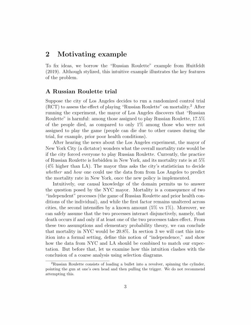
To represent the two causes of death, we refine our model by defining twoextra random variables, B and H: (i) B denotes “bad luck” when playingRussian Roulette, and its values represent a match (B = 1) or mismatch(B = 0) between the trigger and the location of the bullet in the cylinder;(ii) and H denotes all other health factors producing death (H = 1) orsurvival (H = 0). Accordingly, our causal diagram will contain two newedges, H → Y and B → Y , since both “health conditions” and “bad luck”are key determinants of mortality Y . The updated causal diagram is shown
5
YX
B H
(a) Causal diagram
YX
B H
S
(b) Selection diagram
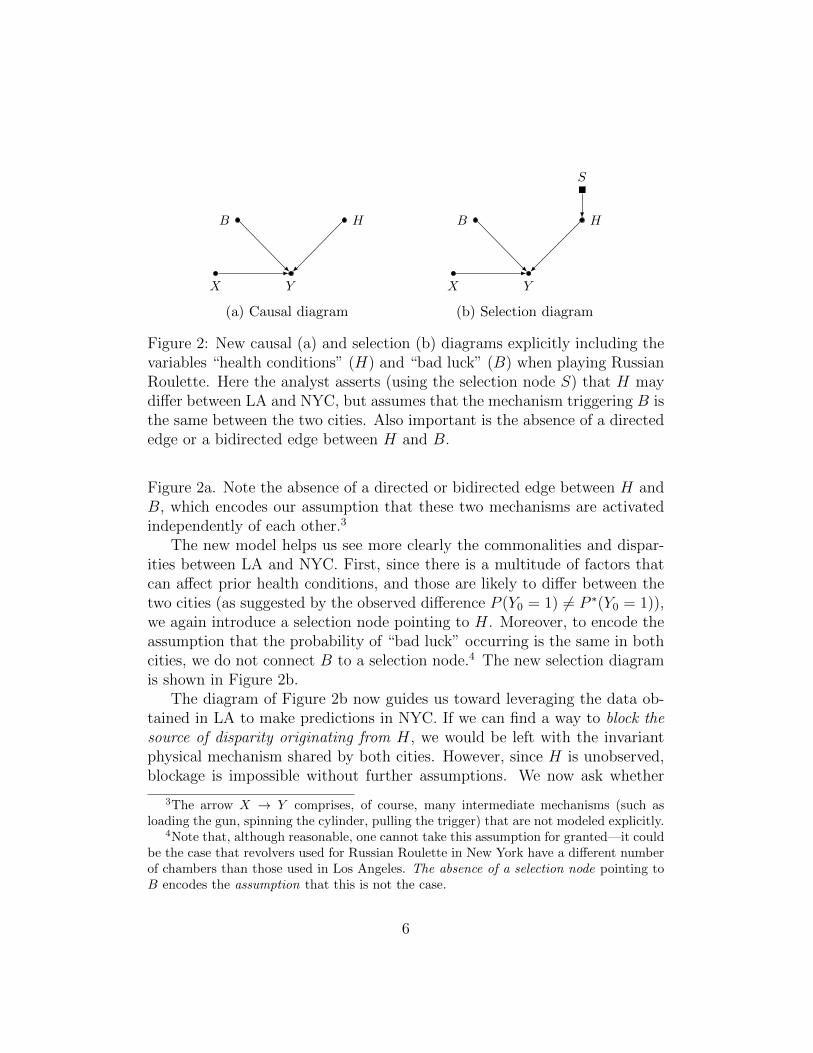
Figure 2: New causal (a) and selection (b) diagrams explicitly including thevariables “health conditions” (H) and “bad luck” (B) when playing RussianRoulette. Here the analyst asserts (using the selection node S) that H maydiffer between LA and NYC, but assumes that the mechanism triggering B isthe same between the two cities. Also important is the absence of a directededge or a bidirected edge between H and B.
Figure 2a. Note the absence of a directed or bidirected edge between H andB, which encodes our assumption that these two mechanisms are activatedindependently of each other.3
The new model helps us see more clearly the commonalities and dispar-ities between LA and NYC. First, since there is a multitude of factors thatcan affect prior health conditions, and those are likely to differ between thetwo cities (as suggested by the observed difference P (Y0 = 1) 6= P ∗(Y0 = 1)),we again introduce a selection node pointing to H. Moreover, to encode theassumption that the probability of “bad luck” occurring is the same in bothcities, we do not connect B to a selection node.4 The new selection diagramis shown in Figure 2b.
The diagram of Figure 2b now guides us toward leveraging the data ob-tained in LA to make predictions in NYC. If we can find a way to block thesource of disparity originating from H, we would be left with the invariantphysical mechanism shared by both cities. However, since H is unobserved,blockage is impossible without further assumptions. We now ask whether
3The arrow X → Y comprises, of course, many intermediate mechanisms (such asloading the gun, spinning the cylinder, pulling the trigger) that are not modeled explicitly.
4Note that, although reasonable, one cannot take this assumption for granted—it couldbe the case that revolvers used for Russian Roulette in New York have a different numberof chambers than those used in Los Angeles. The absence of a selection node pointing toB encodes the assumption that this is not the case.
6
our understanding of how the two mechanisms interact in producing Y wouldpermit us to estimate P ∗(Y1 = 1).
Leveraging functional constraints
Our understanding that mortality is caused by either one of the two processes(prior health conditions or bad luck in the game), dictates the followingfunctional specification for the structural equation of Y ,
Y = H ∨ (X ∧B) (1)
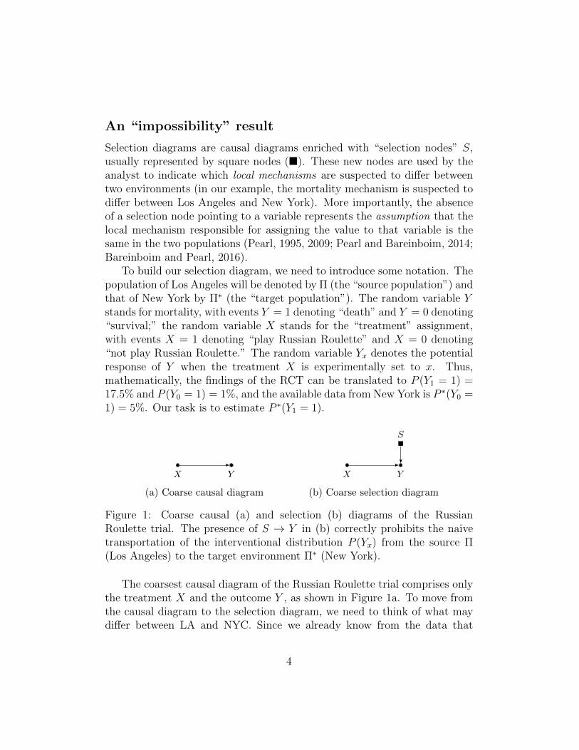
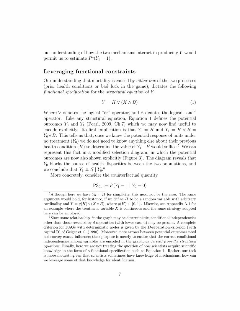
Where ∨ denotes the logical “or” operator, and ∧ denotes the logical “and”operator. Like any structural equation, Equation 1 defines the potentialoutcomes Y0 and Y1 (Pearl, 2009, Ch.7) which we may now find useful toencode explicitly. Its first implication is that Y0 = H and Y1 = H ∨ B =Y0∨B. This tells us that, once we know the potential response of units underno treatment (Y0) we do not need to know anything else about their previoushealth condition (H) to determine the value of Y1—B would suffice.5 We canrepresent this fact in a modified selection diagram, in which the potentialoutcomes are now also shown explicitly (Figure 3). The diagram reveals thatY0 blocks the source of health disparities between the two populations, andwe conclude that Y1 ⊥⊥ S | Y0.
6
More concretely, consider the counterfactual quantity
PS01 := P (Y1 = 1 | Y0 = 0)
5Although here we have Y0 = H for simplicity, this need not be the case. The sameargument would hold, for instance, if we define H to be a random variable with arbitrarycardinality and Y = g(H)∨ (X ∧B), where g(H) ∈ {0, 1}. Likewise, see Appendix A.1 foran example where the treatment variable X is continuous and the same strategy adoptedhere can be employed.
6Since some relationships in the graph may be deterministic, conditional independenciesother than those revealed by d-separation (with lower-case d) may be present. A completecriterion for DAGs with deterministic nodes is given by the D-separation criterion (withcapital D) of Geiger et al. (1990). Moreover, note arrows between potential outcomes neednot convey causal influence; their purpose is merely to ensure that the correct conditionalindependencies among variables are encoded in the graph, as derived from the structuralequations. Finally, here we are not treating the question of how scientists acquire scientificknowledge in the form of a functional specification such as Equation 1. Rather, our taskis more modest: given that scientists sometimes have knowledge of mechanisms, how canwe leverage some of that knowledge for identification.
7
Y
Y1
B
X
Y0
H
S
Figure 3: Selection diagram explicitly showing the potential outcomes Y0 andY1 as implied by the functional constraints. Note that Y1 ⊥⊥ S | Y0.
which stands for the share of people who would die if forced to play Rus-sian Roulette, among those who would not have died if not forced to do so.In other words, PS01 represents the probability that the game of RussianRoulette is sufficient to kill a person during the trial. The acronym PS01
was chosen to emphasize its relation to the “probability of sufficiency” (PS),PS = P (Y1 = 1|Y = 0, X = 0), as defined and analyzed in Pearl (1999) andTian and Pearl (2000). In our context, since the treatment is randomized,the two quantities coincide,
P (Y1 = 1|Y0 = 0) = P (Y1 = 1|Y0 = 0, X = 0) = P (Y1 = 1|Y = 0, X = 0)
where the first equality is licensed by the randomization of X and the secondequality is due to consistency. In general, however, PS01 need not be thesame as PS—the later measures the probability of fatal treatment amongthose who, given the choice, would choose not to be treated and survive;the former measures the probability of fatal treatment among those whowould survive had they not been assigned for treatment.7 Similar reasoningholds for PS10 := P (Y1 = 0 | Y0 = 1), which stands for the probability thatplaying Russian Roulette is sufficient to save a person who would die if deniedtreatment. In our example, this probability is obviously zero as we shallformally show below. The condition Y1 ⊥⊥ S | Y0, implied by the diagram,states that these probabilities of causation are invariant across cities.8 This
7For example, in legal settings, where acts are executed by choice, conditioning on theobserved X gives a more appropriate measure of an agent’s responsibility, as argued inPearl (2009, Ch. 9) and Pearl (2015).
8Probabilities of causation have been extensively studied elsewhere under a differentcontext. See Pearl (1999); Tian and Pearl (2000); Pearl (2009).
8
feature of invariance, which is important in its own right, follows solely fromour structural assumption about the mechanisms involved.
A second implication of Equation 1 is that the treatment effect is mono-tonic, that is Y1 ≥ Y0 for all individuals. This, in turn, implies PS10 = 0; inother words, an individual that would have died of other causes during thetrial, would still die if forced to play Russian Roulette. It has been shownthat monotonicity is sufficient for identifying PS01 in this setting (Pearl,1999; Tian and Pearl, 2000; Huitfeldt et al., 2018). Indeed, by the law oftotal probability,
P (Y1 = 1) = (1− PS10)P (Y0 = 1) + PS01(1− P (Y0 = 1))
The quantity P (Y0 = 1) is given from the RCT (1%) and, due to monotonic-ity, PS10 = 0. Thus, we have:
PS01 =P (Y1 = 1)− P (Y0 = 1)
1− P (Y0 = 1)=
17.5%− 1%
99%= 1/6
This is not surprising; the probability that the “treatment” is sufficient tokill an individual who would have otherwise survived indeed equals 1/6—theprobability of having “bad luck” in the game of Russian Roulette, using arevolver with six chambers.9
Thus far we have established that PS10 = PS∗10, PS01 = PS∗
01, and thatPS10 = 0, PS01 = 1/6. Combining these results with the current baselinemortality from NYC, that is, P ∗(Y0 = 1) = 5%, we can finally evaluate ourtarget quantity P ∗(Y1 = 1),
P ∗(Y1 = 1) = (1− PS∗10)P
∗(Y0 = 1) + PS∗01(1− P ∗(Y0 = 1))
= (1− PS10)(5%) + PS01(95%)
= (1)(5%) + (1/6)(95%) = 20.8%
9The right-hand side of this expression is known as the “relative difference,” or “suscep-
tibility.” Simple algebra shows that P (Y1=1)−P (Y0=1)1−P (Y0=1) = 1− 1−P (Y1=1)
1−P (Y0=1) , where the quantity1−P (Y1=1)1−P (Y0=1) is known as the “survival ratio.” Since under the assumption of monotonicity
these estimands identify PS01, and PS01 is invariant across domains, it thus follows thatthe “relative difference” and the “survival ratio” will also be equal between populations.Huitfeldt et al. (2018) suggested using this fact as a rationale for assuming homogeneityof effect measures across domains, a common heuristic among epidemiologists for ap-proaching generalizability problems. These equivalences, however, break down withoutmonotonicity; in that case, the “relative difference” is a lower bound for the probabilityof sufficiency (Tian and Pearl, 2000), as we discuss next.
9
Which matches the intuitive answer obtained in Section 2.As a brief remark, note that, if instead of Y1 ⊥⊥ S | Y0 we had obtained
the condition Y0 ⊥⊥ S | Y1, we would conclude that the probabilities PN01 :=P (Y0 = 0 | Y1 = 1) and PN10 := P (Y0 = 0 | Y1 = 1) are the same across trials.These quantities represent the probability that the treatment is necessary forcausing (PN01) or preventing (PN10) the outcome during the experiment. Allresults of this paper hold in this setting, with minor modifications. Therefore,for simplicity of exposition, in the remainder of the text we discuss the caseof Y1 ⊥⊥ S | Y0 only.10
Bounds without monotonicity
A key step in obtaining a point estimate for P ∗(Y1 = 1) was the mono-tonicity property, which emanates from the functional form of Equation 1.Monotonicity allowed us to identify the probabilities of sufficiency PS01 andPS10, which, as advertised by the assumptions in the selection diagram ofFigure 3, are invariant across domains. The monotonicity property holdstrivially in our example of the Russian Roulette, when Y represents death,but it may not hold for other outcomes or, more generally, it may not holdin contexts beyond our stylized example.
Remarkably, however, even in the absence of monotonicity, one can stillassess the transported causal effect, albeit in the form of a bound. Thenext theorem shows that the counterfactual independence Y1 ⊥⊥ S | Y0 byitself is strong enough for bounding the causal effect in the target domain.These results improve the bias analysis performed by Huitfeldt et al. (2018),and provide an exact characterization of the inferences compatible with theassumption of Y1 ⊥⊥ S | Y0.
Theorem 1. Consider a source domain Π and a target domain Π∗. Let Pij :=P (Yi = j), P ∗
ij := P ∗(Yi = j), and let RR = P11
P01denote the risk-ratio in the
trial of the source domain Π. If Y1 ⊥⊥ S | Y0, then P ∗11 of Π∗ is bounded by
10For example, under the assumption of monotonicity, we have that PN01 =P (Y1=1)−P (Y0=1)
P (Y1=1) (Pearl, 1999). This last estimand is known as the “excess-risk-ratio,”
and algebra also shows that P (Y1=1)−P (Y0=1)P (Y1=1) = 1− 1
P (Y1=1)/P (Y0=1) , where P (Y1=1)P (Y0=1) is the
“risk ratio.” Thus in this setting, both the “excess-risk-ratio” and the “risk ratio” wouldbe equal across domains. Without monotonicity, the “excess-risk-ratio” is a lower boundon the probability of necessity (Tian and Pearl, 2000).
10

P ∗L11 ≤ P ∗
11 ≤ P ∗U11 , with,
P ∗L11 = RR× P ∗
01 + min
{(P01 − P ∗
01
P01
)PSL
01,
(P01 − P ∗
01
P01
)PSU
01
},
P ∗U11 = RR× P ∗
01 + max
{(P01 − P ∗
01
P01
)PSL
01,
(P01 − P ∗
01
P01
)PSU
01
}where PSL
01 = max{
0, P11−P01
1−P01
}and PSU
01 = min{
P11
1−P01, 1}
are the lower and
upper bounds on PS01, respectively.
Proof. The bounds are obtained by solving a linear optimization problem, asdetailed in Appendix A.2.
Theorem 1 can be better understood as a two-stage process. First, witha little algebra, it is possible to re-express P ∗(Y1 = 1) as a function of PS01
alone, resulting in,
P ∗(Y1 = 1) = RR× P ∗(Y0 = 1) +
(P (Y0 = 1)− P ∗(Y0 = 1)
P (Y0 = 1)
)PS01 (2)
Where RR = P (Y1 = 1)/P (Y0 = 1) denotes the risk-ratio obtained in thetrial of the source domain Π. The first term of this expression, RR×P ∗(Y0 =1), consists of the “naive” prediction for P ∗(Y1 = 1) that one would haveobtained by assuming a constant risk ratio across populations. The secondterm adjusts this naive prediction, by taking into account both the excessrisk-ratio of contrasting the baseline mortality between Π and Π∗, as well asthe probability of sufficiency shared across environments, PS01.
After this, note that, although the probability of sufficiency PS01 in Equa-tion 2 cannot be point identified, it can be bounded by (see Appendix A.2as well as Tian and Pearl (2000))
max
{0,
P (Y1 = 1)− P (Y0 = 1)
1− P (Y0 = 1)
}≤ PS01 ≤ min
{P (Y1 = 1)
1− P (Y0 = 1), 1
}(3)
Thus, by substituting PS01 with its bounds, we obtain the desired boundsfor the target quantity P ∗(Y1 = 1).
For instance, in our Russian Roulette example, regardless of whethermonotonicity holds, PS01 can be bounded by
16.7% ≤ PS01 ≤ 17.7%
11
And this assures us that P ∗(Y1 = 1) must lie between,
16.8% ≤ P ∗(Y1 = 1) ≤ 20.8%
To put it another way, the results of the trial in LA tells us that implementingthe policy in NYC would cause at least an increase of 16.8%− 5% = 11.8%and at most an increase of 20.8% − 5% = 15.8% in mortality. Note that,here, substituting the lower bound for PS01 (16.7%) actually translates tothe upper bound for P ∗(Y1 = 1) (20.8%). This happens because the baselinerisk in the target population Π∗ is higher than that of the source populationΠ, and thus the adjustment due to PS01, in Equation 2, is negative.
These considerations naturally lead to the question: in general, how in-formative are the bounds on P ∗(Y1 = 1)? It turns out that the width ofthe bounds have a simple characterization. Consider the case in which thebounds for PS01 are not zero nor one. Now let P ∗U(Y1 = 1) and P ∗L(Y1 = 1)denote the upper and lower bound on P ∗(Y1 = 1), respectively. After somealgebra, it is possible to show that (see Appendix A.2),
P ∗U(Y1 = 1)− P ∗L(Y1 = 1) =|P (Y0 = 1)− P ∗(Y0 = 1)|
1− P (Y0 = 1)(4)
That is, in this setting, the width of the bounds depends on the baselinerisks P (Y0 = 1) and P ∗(Y0 = 1) alone. Moreover, even if the bounds for PS01
happen to be “wide,” if the baseline risks are close enough across populations,the bounds for P ∗(Y1 = 1) can still be “narrow.” In Section 4 we illustratethis fact with a real data example in which the bounds are narrow enoughto imply a positive effect of the treatment.
Identification with trials from multiple source domains
In Theorem 1 we learned that the existence of experimental data from onesource population leads to bounds on the transported causal effect of thetarget population, although it is not enough for its point identification. Sur-prisingly, however, if we can obtain experimental data from an additionalsource population, this suffices to change the picture. With two source tri-als, it is possible to obtain a point estimate for the probabilities of sufficiency,and, consequently, for P ∗(Y1 = 1) without invoking monotonicity, nor anyfurther assumptions beyond Y1 ⊥⊥ S | Y0. Moreover, multiple source trials en-
12
tail strong testable implications that can be used to falsify this “cross-world”assumption.11
To illustrate, consider our Russian Roulette example, and suppose welearn that the city of Chicago has also performed an RCT. In that trial,25% of those assigned to play the game died, in contrast to 10% of thosenot assigned to play. If the selection diagram contrasting NYC with Chicagois the same as that of Figure 3, we can combine the results from LA andChicago to estimate the probabilities of sufficiency shared across cities. Bythe law of total probability, expand the expression for P (Y1 = 1), both forLA and Chicago, to obtain a system of two equations and two unknowns:
(LA Equation): 0.175 = (1− PS10)× 0.01 + PS01 × 0.99 (5)
(Chicago Equation): 0.250 = (1− PS10)× 0.10 + PS01 × 0.90 (6)
This system can then be solved for PS10 and PS01
PS10 = 0, PS01 = 1/6
Put differently, the only values for PS10 and PS01 that are compatiblewith the observed data from both trials (LA and Chicago) are that: (i) the“treatment” cannot save anyone from dying; and, that (ii) the treatmentkills 1/6 of those who would not have died otherwise. These are the samenumeric values as before, but with an important difference—we did not as-sume monotonicity to obtain point identification; instead, we learned fromthe data that the treatment effect must be monotonic. Once we have thesenumbers, we can use the same strategy as before to predict the causal effectin NYC, which amounts to, again, 20.8%.
Furthermore, since PS10 and PS01 must be valid probabilities, not allobserved values are compatible with the assumption that Y1 ⊥⊥ S | Y0. Forinstance, suppose that instead of 10%, the observed baseline mortality ratein Chicago were 5%. This would imply the impossible value PS10 = −1.03,thus falsifying the assumption of invariance across domains. It is also easyto see that with three or more source domains we obtain over-identification,since each population pair implies different estimates for PS10 and PS01.If those estimates are discordant, this calls into question the assumption
11Similar observations regarding testable implications when combining information frommultiple studies have also been made in Hartman et al. (2015), Lu et al. (2019) andDahabreh et al. (2020).
13
of Y1 ⊥⊥ S | Y0. These results are somewhat reassuring. They tell us that,despite its “cross-world” nature, the assumption of invariance of probabilitiesof causation across domains may have strong testable implications, and canthus be subjected to empirical scrutiny.
We formalize the previous considerations with the next two theorems.
Theorem 2. Consider two source domains Πa and Πb. Let the probabilitiesof sufficiency be the same across the two populations, that is, PSa
01 = PSb01 =
PS01 and PSa10 = PSb
10 = PS10. Then,
PS10 = 1− P a11P
b00 − P b
11Pa00
P a01P
b00 − P b
01Pa00
PS01 =P b11P
a01 − P a
11Pb01
P a01P
b00 − P b
01Pa00
Where P aij := P a(Yi = j) and P b
ij := P b(Yi = j). Moreover, the experimentalprobabilities of necessity, and probability of necessity and sufficiency (Tianand Pearl, 2000) of both populations are also identifiable from experimentaldata of Πa and Πb.
Proof. As explained in the text, we can use the law of total probability foreach domain to obtain two linear equations with two unknowns, PS01 andPS10. We can thus (generically) solve the system of equations for those quan-tities. Interestingly, in this setting, not only the probabilities of sufficiency,but all remaining probabilities of causation (as discussed in Tian and Pearl(2000)), are also identifiable. See details in Appendix A.2.
Next, the causal effect for a target population Π∗ can be transported byappealing again to the law of total probability.
Theorem 3. Consider two source domains Πa, Πb, and a target domain Π∗.Let the probabilities of sufficiency be the same across populations, that is,PSa
01 = PSb01 = PS∗
01 and PSa10 = PSb
10 = PS∗10. Then, the causal effect P ∗
11 inΠ∗ is given by,
P ∗11 =
P a11P
b00 − P b
11Pa00
P a01P
b00 − P b
01Pa00
× P ∗01 +
P b11P
a01 − P a
11Pb01
P a01P
b00 − P b
01Pa00
× P ∗00
14
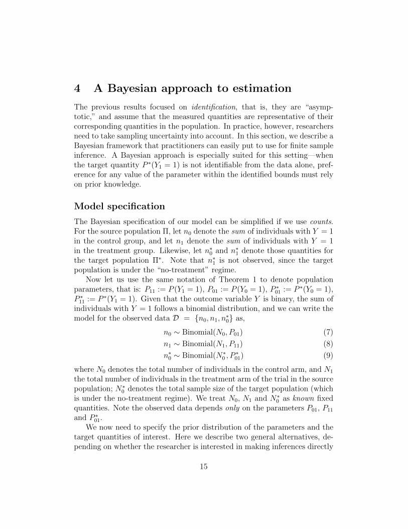
4 A Bayesian approach to estimation
The previous results focused on identification, that is, they are “asymp-totic,” and assume that the measured quantities are representative of theircorresponding quantities in the population. In practice, however, researchersneed to take sampling uncertainty into account. In this section, we describe aBayesian framework that practitioners can easily put to use for finite sampleinference. A Bayesian approach is especially suited for this setting—whenthe target quantity P ∗(Y1 = 1) is not identifiable from the data alone, pref-erence for any value of the parameter within the identified bounds must relyon prior knowledge.
Model specification
The Bayesian specification of our model can be simplified if we use counts.For the source population Π, let n0 denote the sum of individuals with Y = 1in the control group, and let n1 denote the sum of individuals with Y = 1in the treatment group. Likewise, let n∗
0 and n∗1 denote those quantities for
the target population Π∗. Note that n∗1 is not observed, since the target
population is under the “no-treatment” regime.Now let us use the same notation of Theorem 1 to denote population
parameters, that is: P11 := P (Y1 = 1), P01 := P (Y0 = 1), P ∗01 := P ∗(Y0 = 1),
P ∗11 := P ∗(Y1 = 1). Given that the outcome variable Y is binary, the sum of
individuals with Y = 1 follows a binomial distribution, and we can write themodel for the observed data D = {n0, n1, n
∗0} as,
n0 ∼ Binomial(N0, P01) (7)
n1 ∼ Binomial(N1, P11) (8)
n∗0 ∼ Binomial(N∗
0 , P∗01) (9)
where N0 denotes the total number of individuals in the control arm, and N1
the total number of individuals in the treatment arm of the trial in the sourcepopulation; N∗
0 denotes the total sample size of the target population (whichis under the no-treatment regime). We treat N0, N1 and N∗
0 as known fixedquantities. Note the observed data depends only on the parameters P01, P11
and P ∗01.
We now need to specify the prior distribution of the parameters and thetarget quantities of interest. Here we describe two general alternatives, de-pending on whether the researcher is interested in making inferences directly
15
P01
n0
P11
n1
PS10
P ∗11
PS01
P ∗01
n∗0
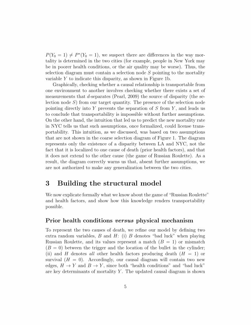
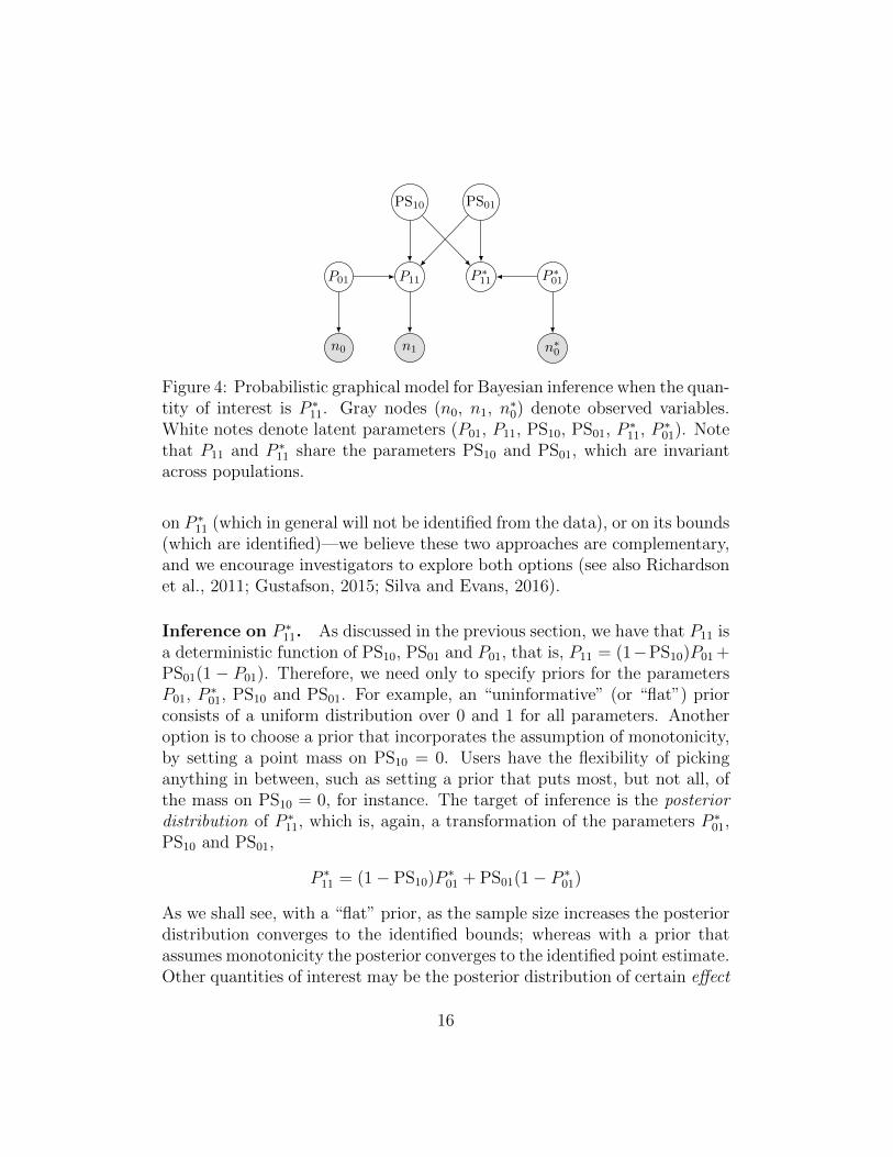
Figure 4: Probabilistic graphical model for Bayesian inference when the quan-tity of interest is P ∗
11. Gray nodes (n0, n1, n∗0) denote observed variables.
White notes denote latent parameters (P01, P11, PS10, PS01, P∗11, P
∗01). Note
that P11 and P ∗11 share the parameters PS10 and PS01, which are invariant
across populations.
on P ∗11 (which in general will not be identified from the data), or on its bounds
(which are identified)—we believe these two approaches are complementary,and we encourage investigators to explore both options (see also Richardsonet al., 2011; Gustafson, 2015; Silva and Evans, 2016).
Inference on P ∗11. As discussed in the previous section, we have that P11 is
a deterministic function of PS10, PS01 and P01, that is, P11 = (1−PS10)P01 +PS01(1 − P01). Therefore, we need only to specify priors for the parametersP01, P
∗01, PS10 and PS01. For example, an “uninformative” (or “flat”) prior
consists of a uniform distribution over 0 and 1 for all parameters. Anotheroption is to choose a prior that incorporates the assumption of monotonicity,by setting a point mass on PS10 = 0. Users have the flexibility of pickinganything in between, such as setting a prior that puts most, but not all, ofthe mass on PS10 = 0, for instance. The target of inference is the posteriordistribution of P ∗
11, which is, again, a transformation of the parameters P ∗01,
PS10 and PS01,
P ∗11 = (1− PS10)P
∗01 + PS01(1− P ∗
01)
As we shall see, with a “flat” prior, as the sample size increases the posteriordistribution converges to the identified bounds; whereas with a prior thatassumes monotonicity the posterior converges to the identified point estimate.Other quantities of interest may be the posterior distribution of certain effect
16
measures, such as the risk difference RD∗ = P ∗11 − P ∗
01 or the risk ratioRR∗ = P ∗
11/P∗01. Figure 4 shows the probabilistic graphical model of this
setup, with observed variables in gray, and latent parameters in white. Theknown fixed parameters N0, N1 and N∗
0 are omitted for clarity.
Inference on bounds. When making inferences on P ∗11 (which is not iden-
tified), the shape of its posterior will be dependent on (but not completelydetermined by) the shape of the prior of the unidentified quantities PS01 andPS10, regardless of sample size. For this reason, users may also find useful toperform inference directly on the bounds P ∗L
11 and P ∗U11 (which are identified).
While the previous framework can still be used for such inferences, we notethat, if interest lies on the bounds alone, there is a simpler alternative—asthe bounds are functionals of the observed data, inference about P ∗L
11 and P ∗U11
only requires priors on the identified parameters P01, P11 and P ∗01 (Richardson
et al., 2011; Silva and Evans, 2016).
Sampling. Given the observed data D and a prior distribution on theparameters, one can obtain the posterior distribution of the target quantitiesusing Gibbs sampling. Here we use the Gibbs sampler JAGS (Plummeret al., 2003). Extending the model to two (or more) source populationsfollows the same logic, thus we defer its discussion to Appendix A.4. Next, wedemonstrate the method using: (i) simulated data from the Russian Rouletteexample; and, (ii) real data from trials that investigate the effects of vitaminA supplementation on childhood mortality. Code for replicating all resultsis also provided in Appendix A.4.
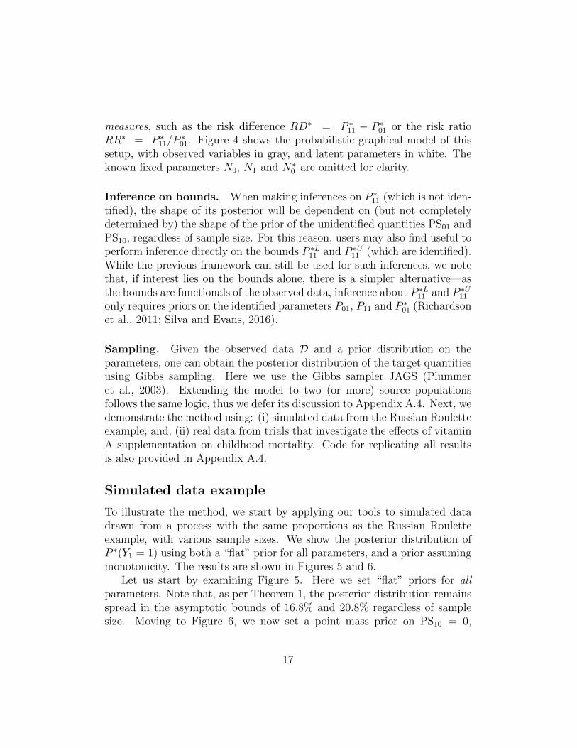
Simulated data example
To illustrate the method, we start by applying our tools to simulated datadrawn from a process with the same proportions as the Russian Rouletteexample, with various sample sizes. We show the posterior distribution ofP ∗(Y1 = 1) using both a “flat” prior for all parameters, and a prior assumingmonotonicity. The results are shown in Figures 5 and 6.
Let us start by examining Figure 5. Here we set “flat” priors for allparameters. Note that, as per Theorem 1, the posterior distribution remainsspread in the asymptotic bounds of 16.8% and 20.8% regardless of samplesize. Moving to Figure 6, we now set a point mass prior on PS10 = 0,
17
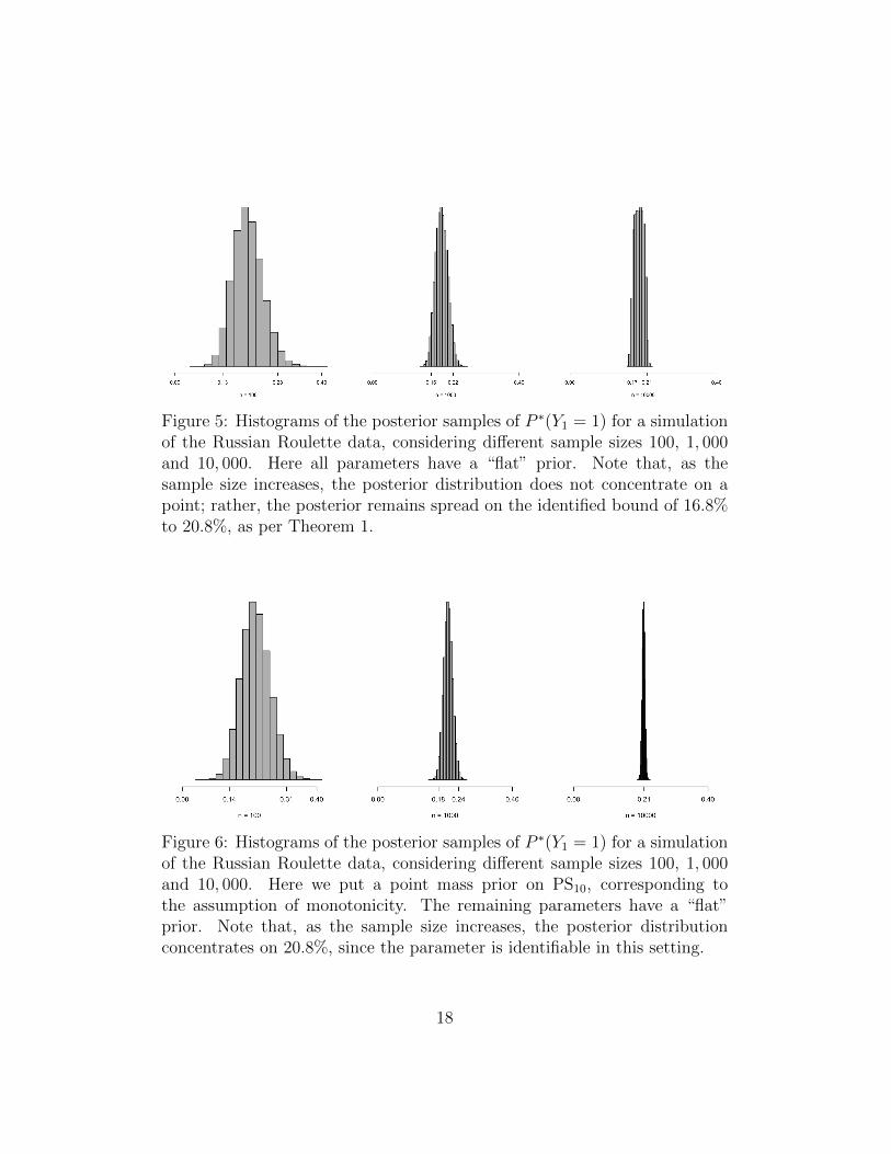
Figure 5: Histograms of the posterior samples of P ∗(Y1 = 1) for a simulationof the Russian Roulette data, considering different sample sizes 100, 1, 000and 10, 000. Here all parameters have a “flat” prior. Note that, as thesample size increases, the posterior distribution does not concentrate on apoint; rather, the posterior remains spread on the identified bound of 16.8%to 20.8%, as per Theorem 1.
Figure 6: Histograms of the posterior samples of P ∗(Y1 = 1) for a simulationof the Russian Roulette data, considering different sample sizes 100, 1, 000and 10, 000. Here we put a point mass prior on PS10, corresponding tothe assumption of monotonicity. The remaining parameters have a “flat”prior. Note that, as the sample size increases, the posterior distributionconcentrates on 20.8%, since the parameter is identifiable in this setting.
18
representing the assumption of monotonicity. The remaining parameterscontinue to have a “flat” prior. As expected, the posterior distribution nowconcentrates around 20.8% as the number of cases increases.
Real data example
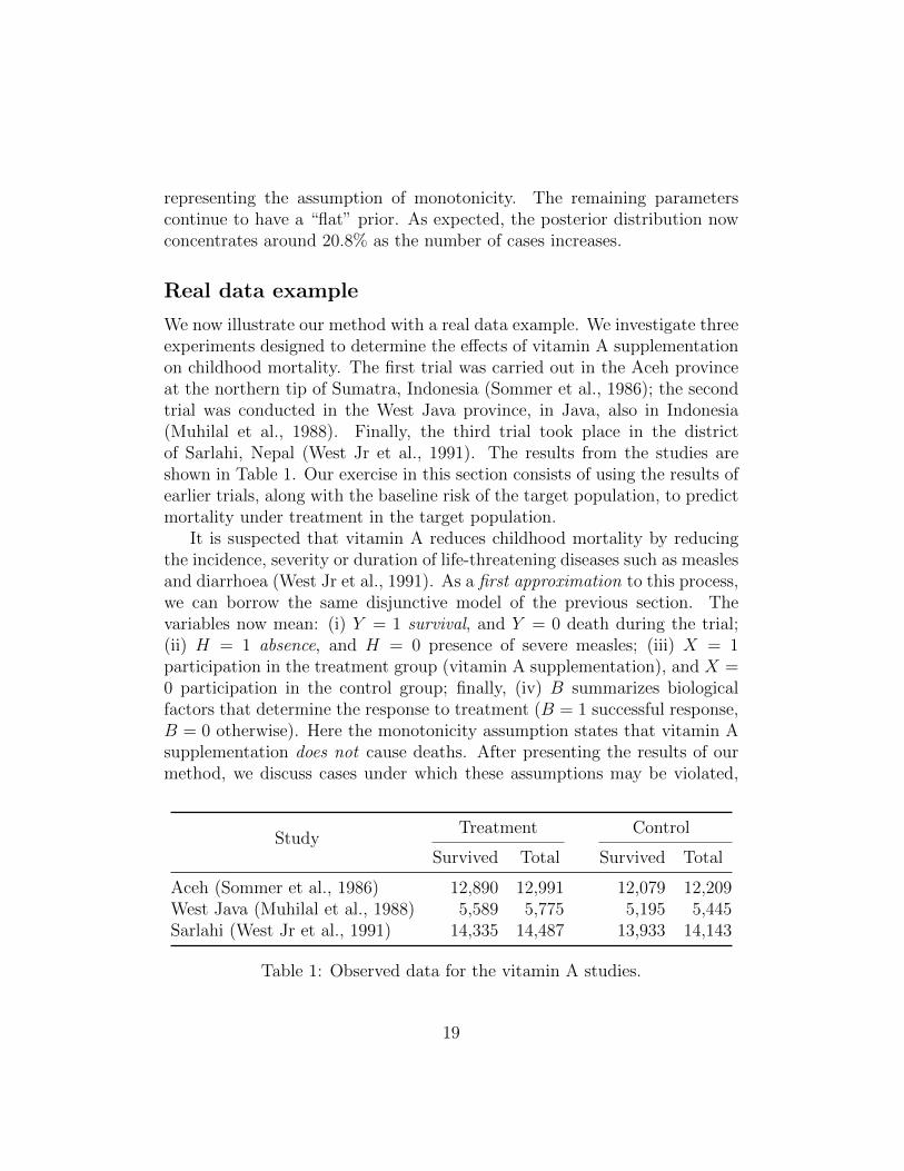
We now illustrate our method with a real data example. We investigate threeexperiments designed to determine the effects of vitamin A supplementationon childhood mortality. The first trial was carried out in the Aceh provinceat the northern tip of Sumatra, Indonesia (Sommer et al., 1986); the secondtrial was conducted in the West Java province, in Java, also in Indonesia(Muhilal et al., 1988). Finally, the third trial took place in the districtof Sarlahi, Nepal (West Jr et al., 1991). The results from the studies areshown in Table 1. Our exercise in this section consists of using the results ofearlier trials, along with the baseline risk of the target population, to predictmortality under treatment in the target population.
It is suspected that vitamin A reduces childhood mortality by reducingthe incidence, severity or duration of life-threatening diseases such as measlesand diarrhoea (West Jr et al., 1991). As a first approximation to this process,we can borrow the same disjunctive model of the previous section. Thevariables now mean: (i) Y = 1 survival, and Y = 0 death during the trial;(ii) H = 1 absence, and H = 0 presence of severe measles; (iii) X = 1participation in the treatment group (vitamin A supplementation), and X =0 participation in the control group; finally, (iv) B summarizes biologicalfactors that determine the response to treatment (B = 1 successful response,B = 0 otherwise). Here the monotonicity assumption states that vitamin Asupplementation does not cause deaths. After presenting the results of ourmethod, we discuss cases under which these assumptions may be violated,
StudyTreatment Control
Survived Total Survived Total
Aceh (Sommer et al., 1986) 12,890 12,991 12,079 12,209West Java (Muhilal et al., 1988) 5,589 5,775 5,195 5,445Sarlahi (West Jr et al., 1991) 14,335 14,487 13,933 14,143
Table 1: Observed data for the vitamin A studies.
19
thus preventing one from inferring Y1 ⊥⊥ S | Y0.Our first task is to use the results of the Aceh trial (ΠA) to predict the
effects of the West Java trial (ΠWJ). The estimates of the Aceh trial are
PA(Y1 = 1) = 0.992 and PA(Y0 = 1) = 0.989; whereas the baseline risk in the
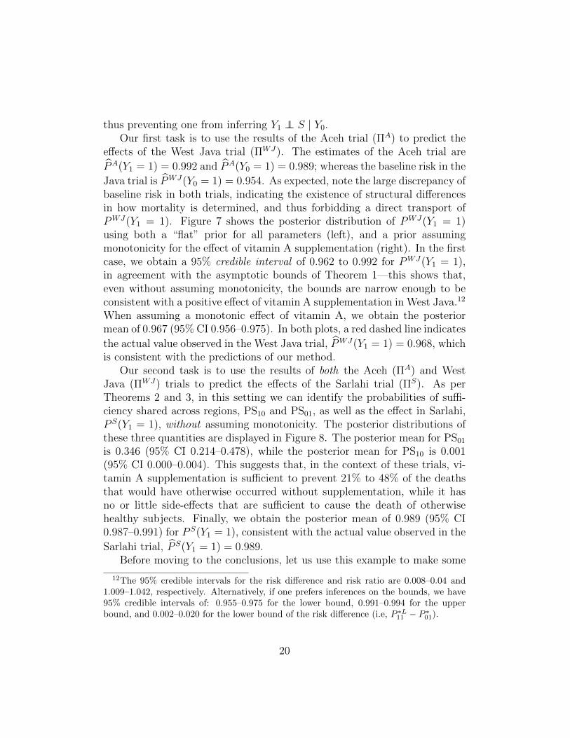
Java trial is PWJ(Y0 = 1) = 0.954. As expected, note the large discrepancy ofbaseline risk in both trials, indicating the existence of structural differencesin how mortality is determined, and thus forbidding a direct transport ofPWJ(Y1 = 1). Figure 7 shows the posterior distribution of PWJ(Y1 = 1)using both a “flat” prior for all parameters (left), and a prior assumingmonotonicity for the effect of vitamin A supplementation (right). In the firstcase, we obtain a 95% credible interval of 0.962 to 0.992 for PWJ(Y1 = 1),in agreement with the asymptotic bounds of Theorem 1—this shows that,even without assuming monotonicity, the bounds are narrow enough to beconsistent with a positive effect of vitamin A supplementation in West Java.12
When assuming a monotonic effect of vitamin A, we obtain the posteriormean of 0.967 (95% CI 0.956–0.975). In both plots, a red dashed line indicates
the actual value observed in the West Java trial, PWJ(Y1 = 1) = 0.968, whichis consistent with the predictions of our method.
Our second task is to use the results of both the Aceh (ΠA) and WestJava (ΠWJ) trials to predict the effects of the Sarlahi trial (ΠS). As perTheorems 2 and 3, in this setting we can identify the probabilities of suffi-ciency shared across regions, PS10 and PS01, as well as the effect in Sarlahi,P S(Y1 = 1), without assuming monotonicity. The posterior distributions ofthese three quantities are displayed in Figure 8. The posterior mean for PS01
is 0.346 (95% CI 0.214–0.478), while the posterior mean for PS10 is 0.001(95% CI 0.000–0.004). This suggests that, in the context of these trials, vi-tamin A supplementation is sufficient to prevent 21% to 48% of the deathsthat would have otherwise occurred without supplementation, while it hasno or little side-effects that are sufficient to cause the death of otherwisehealthy subjects. Finally, we obtain the posterior mean of 0.989 (95% CI0.987–0.991) for P S(Y1 = 1), consistent with the actual value observed in the
Sarlahi trial, P S(Y1 = 1) = 0.989.Before moving to the conclusions, let us use this example to make some
12The 95% credible intervals for the risk difference and risk ratio are 0.008–0.04 and1.009–1.042, respectively. Alternatively, if one prefers inferences on the bounds, we have95% credible intervals of: 0.955–0.975 for the lower bound, 0.991–0.994 for the upperbound, and 0.002–0.020 for the lower bound of the risk difference (i.e, P ∗L
11 − P ∗01).
20
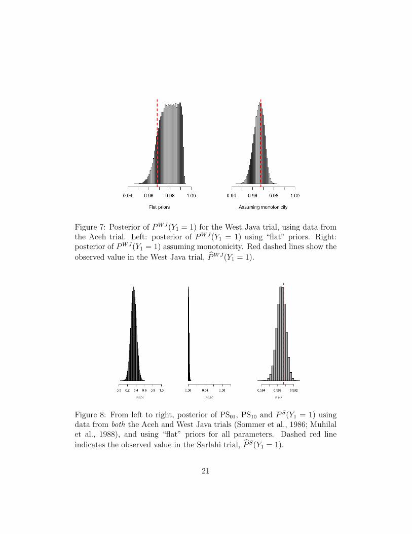
Figure 7: Posterior of PWJ(Y1 = 1) for the West Java trial, using data fromthe Aceh trial. Left: posterior of PWJ(Y1 = 1) using “flat” priors. Right:posterior of PWJ(Y1 = 1) assuming monotonicity. Red dashed lines show the
observed value in the West Java trial, PWJ(Y1 = 1).
Figure 8: From left to right, posterior of PS01, PS10 and P S(Y1 = 1) usingdata from both the Aceh and West Java trials (Sommer et al., 1986; Muhilalet al., 1988), and using “flat” priors for all parameters. Dashed red line
indicates the observed value in the Sarlahi trial, P S(Y1 = 1).
21
brief remarks about causal modeling in practice. Note that the workingmodel in this section assumes the only factor causing deaths during the pe-riod of the trial can be summarized by H, consisting of diseases which, atleast in principle, can be affected by the treatment (e.g, severe measles ordiarrhoea). What happens, however, if we augment the model to allow forother causes of deaths unaffected by vitamin A supplementation? It canbe shown that this new variable is a common cause of both potential re-sponses, thus creating a colliding path and forbidding the conclusion thatY1 ⊥⊥ S | Y0.
13 This suggests caution when transporting these results topopulations where mortality due to diarrhoea or measles is not predominant.
More generally, while one may summarize the main “identification as-sumption” for the results in this paper in terms of the counterfactual inde-pendence Y1 ⊥⊥ S | Y0, note we did not commence the analysis by imposingthis or any “identification assumption.” Instead, we made an effort to expli-cate our understanding of the problem directly in a structural model, and thenecessary counterfactual independence emerged naturally as a logical conse-quence of the structure. This is an important part of the process. If someof those modeling assumptions happen to be challenged, as they often arein practical settings (e.g, unobserved confounding between H and B), weshould refrain from positing that Y1 ⊥⊥ S | Y0 and the model both warns usof possible threats, as well as helps us in finding alternative solutions.14
5 Conclusions
This paper showed how two apparently separate areas of causal inferenceresearch—the generalization of causal effects across populations (Pearl andBareinboim, 2014; Bareinboim and Pearl, 2016; Huitfeldt et al., 2018) andthe identification of “causes of effects” (Pearl, 1999; Tian and Pearl, 2000;Pearl, 2015, 2019)—can be merged for mutual benefit, unveiling importantresults in both areas.
13Call these new causes C. The new structural equation for Y now reads Y = (H ∨(X ∧B))∧¬C. This leads to Y0 = H ∧¬C and Y1 = Y0 ∨ (B ∧¬C). Note this creates thecolliding path S → H → Y0 ← C → Y1, thus forbidding the conclusion that Y1 ⊥⊥ S | Y0,even when there is no selection node pointing directly to C. For another illustration ofwhen collider bias may arise, see Appendix A.3.
14For example, a sensitivity analysis might still be possible, and one could investigatehow big a departure from the original model assumptions would be necessary to invalidatethe main conclusions. See, e.g., Cinelli et al. (2019); Cinelli and Hazlett (2020).
22
The first lesson that emerges from this combined analysis is that certainfunctional constraints may entail the invariance of probabilities of causationacross domains, which can then be used as instruments to license general-ization. This may occur when the outcome is a product of several inde-pendent processes, only some of which are carriers of disparities, and whenthe outcome produced under the “no-treatment” condition is sufficient toblock these sources of disparity. These functional constraints may enable theidentification, or at least the bounding of the target effect in settings wherenon-parametric generalization is otherwise impossible.
A second lesson that surfaces from our investigation is that, wheneverexperimental data from multiple sites are available, these may lead to thepoint identification of probabilities of causation. These counterfactual prob-abilities can be the targets of investigations in public health, legal settings,and the production of explanations (Mueller and Pearl, 2020; Pearl, 2015,2019). For example, drugs with a positive average treatment effect may stillkill individuals who would have otherwise survived—being able to quantifythe percentage of individuals that are saved or harmed by the treatment hasimportant implications in many public health applications.
The development of tools for automating the types of analyses presentedhere, paralleling those available for non-parametric models, is a challeng-ing topic for future work. As we have seen, determining the invariance ofprobabilities of causation requires additional constraints beyond the stan-dard non-parametric model; some recent developments, such as algorithmsfor handling context-specific independencies for causal identification (Tikkaet al., 2019), may provide the initial steps towards this undertaking.
Conflict of interest
The authors declare that they have no conflict of interest.
23
References
E. Bareinboim and J. Pearl. Causal inference and the data-fusion problem.Proceedings of the National Academy of Sciences, 113(27):7345–7352, 2016.
C. Cinelli and C. Hazlett. Making sense of sensitivity: Extending omittedvariable bias. Journal of the Royal Statistical Society: Series B (StatisticalMethodology), 2020.
C. Cinelli, D. Kumor, B. Chen, J. Pearl, and E. Bareinboim. Sensitivityanalysis of linear structural causal models. International Conference onMachine Learning, 2019.
I. J. Dahabreh, L. C. Petito, S. E. Robertson, M. A. Hernan, and J. A.Steingrimsson. Toward causally interpretable meta-analysis: Transportinginferences from multiple randomized trials to a new target population.Epidemiology, 31(3):334–344, 2020.
D. Geiger, T. Verma, and J. Pearl. Identifying independence in bayesiannetworks. Networks, 20(5):507–534, 1990.
A. Gelman, J. B. Carlin, H. S. Stern, D. B. Dunson, A. Vehtari, and D. B.Rubin. Bayesian data analysis. CRC press, 2013.
P. Gustafson. Bayesian inference for partially identified models: Exploringthe limits of limited data, volume 140. CRC Press, 2015.
E. Hartman, R. Grieve, R. Ramsahai, and J. S. Sekhon. From sate to patt:combining experimental with observational studies to estimate populationtreatment effects. Journal of Royal Statistical Society Series A (Statisticsin Society), 10:1111, 2015.
A. Huitfeldt. Effect heterogeneity and external validity in medicine. Availablein: https://www.lesswrong.com/posts/wwbrvumMWhDfeo652/, 2019.
A. Huitfeldt, A. Goldstein, and S. A. Swanson. The choice of effect measurefor binary outcomes: Introducing counterfactual outcome state transitionparameters. Epidemiologic methods, 7(1), 2018.
A. Huitfeldt, S. A. Swanson, M. J. Stensrud, and E. Suzuki. Effect hetero-geneity and variable selection for standardizing causal effects to a targetpopulation. European journal of epidemiology, pages 1–11, 2019.
24

Y. Lu, D. O. Scharfstein, M. M. Brooks, K. Quach, and E. H. Kennedy.Causal inference for comprehensive cohort studies. arXiv preprintarXiv:1910.03531, 2019.
S. Mueller and J. Pearl. Which patients are in greater need: A counterfac-tual analysis with reflections on covid-19. Causal Analysis in Theory andPractice, 2020. Available in: https://ucla.in/39Ey8sU.
P. D. Muhilal, Y. R. Idjradinata, and K. D. Muherdiyantiningsih. Vita-min a-fortified monosodium glutamate and health, growth, and survival ofchildren: a controlled field trial. Am J Clin Nutr, 48(5):1271–1276, 1988.
J. Pearl. Causal diagrams for empirical research. Biometrika, 82(4):669–688,1995.
J. Pearl. Probabilities of causation: three counterfactual interpretations andtheir identification. Synthese, 121(1-2):93–149, 1999.
J. Pearl. Causality. Cambridge university press, 2009.
J. Pearl. Causes of effects and effects of causes. Sociological Methods &Research, 44(1):149–164, 2015.
J. Pearl. Sufficient causes: On oxygen, matches, and fires. Journal of CausalInference, 7(2), 2019.
J. Pearl and E. Bareinboim. External validity: From do-calculus to trans-portability across populations. Statistical Science, 29(4):579–595, 2014.
M. Plummer. rjags: Bayesian graphical models using mcmc. R packageversion, 4(6), 2016.
M. Plummer et al. Jags: A program for analysis of bayesian graphical modelsusing gibbs sampling. In Proceedings of the 3rd international workshop ondistributed statistical computing, volume 124, pages 1–10. Vienna, Austria.,2003.
T. S. Richardson, R. J. Evans, and J. M. Robins. Transparent parameteri-zations of models for potential outcomes. Bayesian Statistics, 9:569–610,2011.
25

R. Silva and R. Evans. Causal inference through a witness protection pro-gram. The Journal of Machine Learning Research, 17(1):1949–2001, 2016.
A. Sommer, E. Djunaedi, A. Loeden, I. Tarwotjo, K. West JR, R. Tilden,L. Mele, A. S. Group, et al. Impact of vitamin a supplementation on child-hood mortality: a randomised controlled community trial. The Lancet, 327(8491):1169–1173, 1986.
J. Tian and J. Pearl. Probabilities of causation: Bounds and identification.Annals of Mathematics and Artificial Intelligence, 28(1-4):287–313, 2000.
S. Tikka, A. Hyttinen, and J. Karvanen. Identifying causal effects via context-specific independence relations. In Advances in Neural Information Pro-cessing Systems, pages 2800–2810, 2019.
K. P. West Jr, J. Katz, S. C. LeClerq, E. Pradhan, J. M. Tielsch, A. Sommer,R. Pokhrel, S. Khatry, S. Shrestha, and M. Pandey. Efficacy of vitamina in reducing preschool child mortality in nepal. The Lancet, 338(8759):67–71, 1991.
26
A Appendix
A.1 An example with continuous treatment
Here we provide a simple example in which, although the treatment variableis continuous, the relevant dependencies among potential outcomes are stillamenable to graphical representation. Suppose we have the same selectiondiagram as in Figure 2b, but now let X, B, and H all be continuous vari-ables. Next, consider the following functional specification for the structuralequation of Y ,
Y = I(H > 0) ∨ I(X ×B > 0) (10)
Where I(·) denotes the indicator function. Now note from Equation 10 wecan derive the potential outcomes Y0 = I(H > 0) for x = 0, and, Yx =I(H > 0) ∨ I(xB > 0) = Y0 ∨ I(xB > 0), for x 6= 0. We can thus draw thesame modified selection diagram as in Figure 3, but now replacing Y1 withYx, leading to the conclusion that Yx ⊥⊥ S | Y0, for all x 6= 0.
A.2 Proofs
A.2.1 Bounds with a single source population
Here we show how to obtain the bounds of Theorem 1. To simplify notation,let Pij := P (Yi = j), P ∗
ij := P ∗(Yi = j), PS10 := P ∗(Y1 = 0|Y0 = 1) =P (Y1 = 0|Y0 = 1) and PS01 = P ∗(Y1 = 1|Y0 = 0) = P (Y1 = 1|Y0 = 0). Thetarget function to be optimized is P ∗
11, which can be written as,
P ∗11 = (1− PS10)P
∗01 + PS01(1− P ∗
01) (11)
Our goal is to pick PS10 and PS01 such that it maximizes (or minimizes)Eq. 11 subject to the following constraints: (i) PS10 and PS01 need to bebetween zero and one (since PS10 and PS01 need to be valid probabilities);and, (ii) PS10 and PS01 must conform to the observed results of the trial inthe source domain, that is, P11 = (1− PS10)P01 + PS01(1− P01). Thus, our
27

optimization problem is,
maxPS10,PS01
P ∗11 = (1− PS10)P
∗01 + PS01(1− P ∗
01)
s.t. P11 = (1− PS10)P01 + PS01(1− P01)
and 0 ≤ PS10 ≤ 1, 0 ≤ PS01 ≤ 1
To simplify the problem, we can use the equality constraint P11 = (1 −PS10)P01 + PS01(1 − P01) to eliminate one of the variables. For instance,writing PS10 in terms of PS01 gives us,
1− PS10 =P11 − PS01(1− P01)
P01
(12)
Which results in a new target function,
P ∗11 = (1− PS10)P
∗01 + PS01(1− P ∗
01) (13)
=
(P11 − PS01(1− P01)
P01
)P ∗01 + PS01(1− P ∗
01) (14)
=
(P11
P01
)P ∗01 +
(P01 − P ∗
01
P01
)PS01 (15)
= RR× P ∗01 +
(P01 − P ∗
01
P01
)PS01 (16)
Where RR = P11
P01is the causal risk-ratio in the trial of the source domain
Π. Since 0 ≤ (1 − PS10) ≤ 1, the substitution also results in additionalconstraints on PS01,
P11 − P01
1− P01
≤ PS01 ≤P11
1− P01
(17)
Thus, define the lower and upper bounds on PS01 as
PSL01 = max
{0,
P11 − P01
1− P01
}, PSU
01 = min
{P11
1− P01
, 1
}
28

Our new maximization problem can be written as,
maxPS01
RR× P ∗01 +
(P01 − P ∗
01
P01
)PS01 s.t. PSL
01 ≤ PS01 ≤ PSU01 (18)
Since the target function is linear, the maximum occurs at the extreme pointsof PS01. The same reasoning holds for the minimization problem. Thus, wehave that,
P ∗L11 ≤ P ∗
11 ≤ P ∗U11
Where,
P ∗L11 = RR× P ∗
01 + min
{(P01 − P ∗
01
P01
)PSL
01,
(P01 − P ∗
01
P01
)PSU
01
}and
P ∗U11 = RR× P ∗
01 + max
{(P01 − P ∗
01
P01
)PSL
01,
(P01 − P ∗
01
P01
)PSU
01
}A.2.2 Informativeness of the bounds
We now derive the width of the bounds for P ∗11 for the case when the bounds
for PS01 do not reach 0 nor 1 (this will happen when both P11 > P01 andP11 < 1− P01). Define the width W of the bounds as the difference betweenthe upper and lower bound of P ∗
11, that is,
W = P ∗U11 − P ∗L
11
29

Expanding the terms we obtain,
W = P ∗U11 − P ∗L
11 (19)
=
∣∣∣∣(P01 − P ∗01
P01
)PSU
01 −(P01 − P ∗
01
P01
)PSL
01
∣∣∣∣ (20)
=|P01 − P ∗
01|P01
×(PSU
01 − PSL01
)(21)
=|P01 − P ∗
01|P01
× P01
1− P01
(22)
=|P01 − P ∗
01|1− P01
(23)
Thus, when the bounds for PS01 are “interior,” the informativeness of thebounds depend only on P01 and P ∗
01. Moreover, even if the bounds for PS01
are “wide,” the bounds for P ∗11 may be “narrow,” provided the baseline risks
of the source and target population are close enough.
A.2.3 Identification with multiple source domains
We now show how to obtain the identification results of Theorem 2 and 3.Consider two source populations Πa and Πb. Again, to simplify notation, letP aij := P a(Yi = j), P b
ij := P a(Yi = j), PS10 := P a(Y1 = 0|Y0 = 1) = P b(Y1 =0|Y0 = 1) = P ∗(Y1 = 0|Y0 = 1) and PS01 := P a(Y1 = 1|Y0 = 0) = P b(Y1 =1|Y0 = 0) = P ∗(Y1 = 1|Y0 = 0).
First note that PS10 and PS01 are identified from the experimental datain Πa and Πb. Using the law of total probability for P a
11 and P b11 write,
P a11 = (1− PS10)× P a
01 + PS01 × P a00 (24)
P b11 = (1− PS10)× P b
01 + PS01 × P b00 (25)
We thus have a system of two equations and two unknowns,[P a01 P a
00
P b01 P b
00
] [(1− PS10)
PS01
]=
[P a11
P b11
](26)
30

Yielding the solution,[(1− PS10)
PS01
]=
1
P a01P
b00 − P b
01Pa00
×[P b00 −P a
00
−P b01 P a
01
] [P a11
P b11
](27)
Which amounts to:
PS10 = 1− P a11P
b00 − P b
11Pa00
P a01P
b00 − P b
01Pa00
(28)
PS01 =P b11P
a01 − P a
11Pb01
P a01P
b00 − P b
01Pa00
(29)
All values of the RHS can be computed from the experimental data of Πa
and Πb. Note that, since PS10 and PS01 must be between 0 and 1, notall solutions are valid. Therefore, two domains already entail some testableimplications—if either PS10 and PS01 are not valid probabilities, this meansthat the assumption that the probabilities of sufficiency are invariant acrossdomains is false. If we add a third or more source domains, it is easy to seethat we will have three or more equations but still only two unknowns, andthe system is thus over-identified.
Once in possession of PS10 and PS01, we can transport of the causal effectto the target population Π∗ by appealing again to the law of total probability,
P ∗11 = (1− PS10)× P ∗
01 + PS01 × P ∗00 (30)
=P a11P
b00 − P b
11Pa00
P a01P
b00 − P b
01Pa00
× P ∗01 +
P b11P
a01 − P a
11Pb01
P a01P
b00 − P b
01Pa00
× P ∗00 (31)
Finally, we note that all probabilities of causation, as discussed in Tianand Pearl (2000), are also identifiable in this setting. First, consider theprobability of necessity and sufficiency, PNS = P (Y1 = 1, Y0 = 0) for Πa.Using the chain rule, PNS can be written as,
P a(Y1 = 1, Y0 = 0) = P a(Y1 = 1 | Y0 = 0)P a(Y0 = 0) (32)
= PS01 × P a(Y0 = 0) (33)
Note PS01 was already identified, and P a(Y0 = 0) is given by the trial datain Πa, thus rendering PNSa identifiable. Similar reasoning holds for Πb.
For the probability of necessity, define PN01 := P (Y0 = 0 | Y1 = 1). Due tothe randomization of X, PN01 coincides with Tian and Pear’s probability of
31

necessity during the trial (not the observational PN), by the same argumentwe provide for PS in the main text. The final step is to note that,
P a(Y0 = 0 | Y1 = 1) =P a(Y0 = 0, Y1 = 1)
P a(Y1 = 1)=
PNSa
P a(Y1 = 1)
The numerator is simply the PNS, which we have already identified, andthe denominator is given by the trial data in Πa. Again, analogous argumentcan be given for Πb.
A.3 Modeling functional constraints
To illustrate the usefulness of explicitly modeling functional constraints in astructural framework, we apply the same modeling strategy of the paper inan example described in Huitfeldt et al. (2018, p. 11):
Consider a team of investigators who are interested in the effect ofantibiotic treatment on mortality in patients with a specific bacterialinfection (. . . ) the investigators believe that the response to this an-tibiotic is completely determined by an unmeasured bacterial gene,such that only those who are infected with a bacterial strain with thisgene respond to treatment. The prevalence of this bacterial gene isequal between populations, because the populations share the samebacterial ecosystem (. . . ) if the investigators further believe that thegene for susceptibility reduces the mortality in the presence of antibi-otics, but has no effect in the absence of antibiotics, they will concludethat G may be equal between populations.
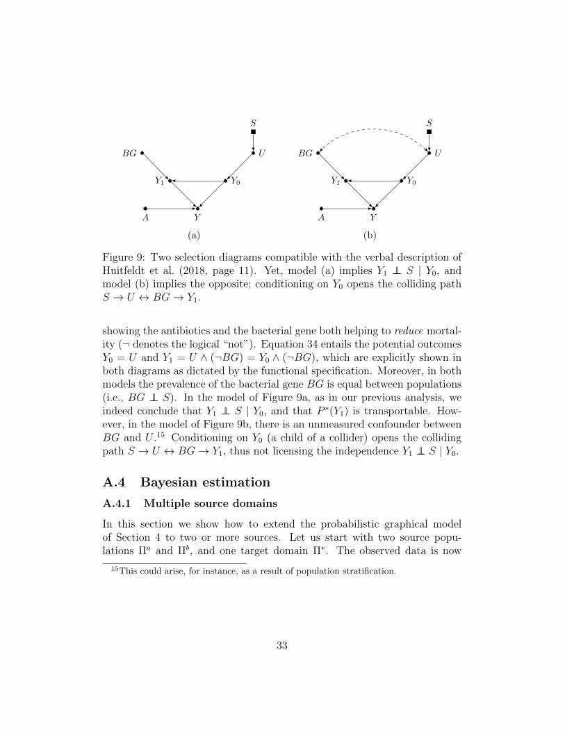
Here the conclusion that G may be equal between populations is equivalentto claiming Y1 ⊥⊥ S | Y0. But is the description above sufficient for substanti-ating this claim? Figure 9 shows two models compatible with the description,yet leading to two opposite conclusions.
Let the variable A represent the binary treatment (antibiotic), Y repre-sent the binary outcome (mortality), BG stand for the presence or absenceof the “bacterial gene” and finally let U be a binary variable that summa-rizes all other factors that may cause death (Y = 1). The description of theproblem suggests the functional specification,
Y = U ∧ (¬A ∨ ¬BG) (34)
32
Y
Y1
BG
A
Y0
U
S
(a)
Y
Y1
BG
A
Y0
U
S
(b)
Figure 9: Two selection diagrams compatible with the verbal description ofHuitfeldt et al. (2018, page 11). Yet, model (a) implies Y1 ⊥⊥ S | Y0, andmodel (b) implies the opposite; conditioning on Y0 opens the colliding pathS → U ↔ BG→ Y1.
showing the antibiotics and the bacterial gene both helping to reduce mortal-ity (¬ denotes the logical “not”). Equation 34 entails the potential outcomesY0 = U and Y1 = U ∧ (¬BG) = Y0 ∧ (¬BG), which are explicitly shown inboth diagrams as dictated by the functional specification. Moreover, in bothmodels the prevalence of the bacterial gene BG is equal between populations(i.e., BG ⊥⊥ S). In the model of Figure 9a, as in our previous analysis, weindeed conclude that Y1 ⊥⊥ S | Y0, and that P ∗(Y1) is transportable. How-ever, in the model of Figure 9b, there is an unmeasured confounder betweenBG and U .15 Conditioning on Y0 (a child of a collider) opens the collidingpath S → U ↔ BG→ Y1, thus not licensing the independence Y1 ⊥⊥ S | Y0.
A.4 Bayesian estimation
A.4.1 Multiple source domains
In this section we show how to extend the probabilistic graphical modelof Section 4 to two or more sources. Let us start with two source popu-lations Πa and Πb, and one target domain Π∗. The observed data is now
15This could arise, for instance, as a result of population stratification.
33
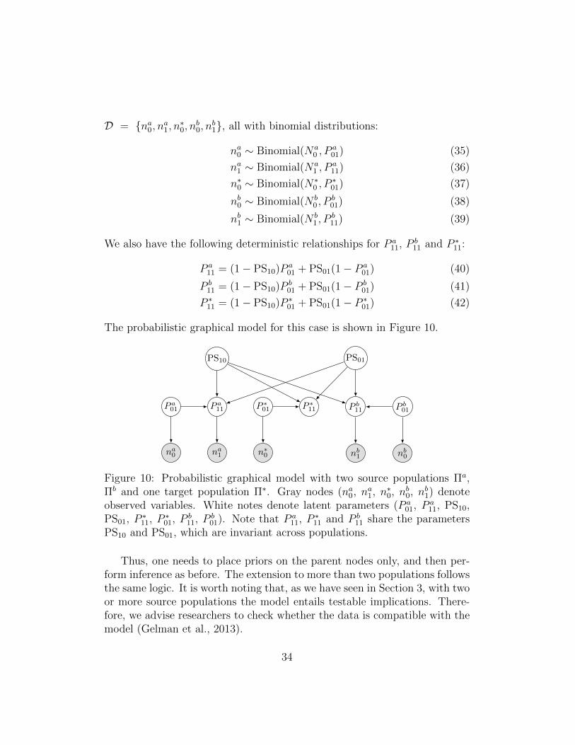
D = {na0, n
a1, n
∗0, n
b0, n
b1}, all with binomial distributions:
na0 ∼ Binomial(Na
0 , Pa01) (35)
na1 ∼ Binomial(Na
1 , Pa11) (36)
n∗0 ∼ Binomial(N∗
0 , P∗01) (37)
nb0 ∼ Binomial(N b
0 , Pb01) (38)
nb1 ∼ Binomial(N b
1 , Pb11) (39)
We also have the following deterministic relationships for P a11, P
b11 and P ∗
11:
P a11 = (1− PS10)P
a01 + PS01(1− P a
01) (40)
P b11 = (1− PS10)P
b01 + PS01(1− P b
01) (41)
P ∗11 = (1− PS10)P
∗01 + PS01(1− P ∗
01) (42)
The probabilistic graphical model for this case is shown in Figure 10.
P a01
na0
P a11
na1
PS10
P ∗01
n∗0
P ∗11 P b
11
PS01
nb1
P b01
nb0
Figure 10: Probabilistic graphical model with two source populations Πa,Πb and one target population Π∗. Gray nodes (na
0, na1, n∗
0, nb0, nb
1) denoteobserved variables. White notes denote latent parameters (P a
01, P a11, PS10,
PS01, P∗11, P
∗01, P
b11, P
b01). Note that P a
11, P∗11 and P b
11 share the parametersPS10 and PS01, which are invariant across populations.
Thus, one needs to place priors on the parent nodes only, and then per-form inference as before. The extension to more than two populations followsthe same logic. It is worth noting that, as we have seen in Section 3, with twoor more source populations the model entails testable implications. There-fore, we advise researchers to check whether the data is compatible with themodel (Gelman et al., 2013).
34

Finally, similarly to the discussion in Section 4, a simpler modeling al-ternative here is to place priors only on the parameters of the observed datadirectly, and make inferences using the posterior of the functionals of theobserved data that identify the target quantities.
A.4.2 Replication code
Here we provide R code to replicate the estimation examples using JAGS(Plummer et al., 2003) and the package rjags (Plummer, 2016).
### Replication code for
### "Generalizing Experimental results
### by Leveraging Knowledge of Mechanisms"
### -- Carlos Cinelli and Judea Pearl
# Set up -------------------------------------------------------
## Cleans workspace
rm(list = ls())
## Loads necessary R packages
library(rjags)
## JAGS models
model_one_source <-
"model{
# Likelihood
n0 ~ dbinom(p01, N0)
n1 ~ dbinom(p11, N1)
n0s ~ dbinom(p01s, N0s)
# Priors
35

PS10 ~ dbeta(1,1)
PS01 ~ dbeta(1,1)
p01 ~ dbeta(1, 1)
p01s ~ dbeta(1, 1)
# Computed quantities
p11 <- (1-PS10)*p01 + PS01*(1-p01)
p11s <- (1-PS10)*p01s + PS01*(1-p01s)
rd <- p11s - p01s
rr <- p11s/p01s
# bounds
PS01_l <- max(0, (p11-p01)/(1-p01))
PS01_u <- min(p11/(1-p01), 1)
p11_1 <- (1-p01s/p01)*PS01_l + (p01s/p01)*p11
p11_2 <- (1-p01s/p01)*PS01_u + (p01s/p01)*p11
p11_l <- min(p11_1, p11_2)
p11_u <- max(p11_1, p11_2)
rd_l <- p11_l - p01s
rr_l <- p11_l/p01s
}"
model_one_source_monotonic <-
"model{
# Likelihood
n0 ~ dbinom(p01, N0)
n1 ~ dbinom(p11, N1)
n0s ~ dbinom(p01s, N0s)
# Priors
PS10 <- 0
PS01 ~ dbeta(1,1)
p01 ~ dbeta(1, 1)
36

p01s ~ dbeta(1, 1)
# Computed quantities
p11 <- (1-PS10)*p01 + PS01*(1-p01)
p11s <- (1-PS10)*p01s + PS01*(1-p01s)
rd <- p11s - p01s
rr <- p11s/p01s
}"
model_two_sources <- "model{
# Likelihood
n0a ~ dbinom(p01a, N0a)
n0b ~ dbinom(p01b, N0b)
n0c ~ dbinom(p01c, N0c)
n1a ~ dbinom(p11a, N1a)
n1b ~ dbinom(p11b, N1b)
# Priors
p01a ~ dbeta(1, 1)
p01b ~ dbeta(1, 1)
p01c ~ dbeta(1, 1)
PS10 ~ dbeta(1, 1)
PS01 ~ dbeta(1, 1)
# Computed quantities
p11a <- (1-PS10)*p01a + PS01*(1-p01a)
p11b <- (1-PS10)*p01b + PS01*(1-p01b)
p11c <- (1-PS10)*p01c + PS01*(1-p01c)
rra <- (p11a)/(p01a)
rrb <- (p11b)/(p01b)
rrc <- (p11c)/(p01c)
}"
37

# Simulated data example ---------------------------------------
loop_n <- c(1e2, 1e3, 1e4)
### Without monotonicity
par(mfrow = c(1, 3))
for(n in loop_n){
# creates data
data <- list(
N0 = n,
n0 = sum(rbinom(n, 1, prob = 0.01)),
N1 = n,
n1 = sum(rbinom(n, 1, prob = 0.175)),
N0s = n,
n0s = sum(rbinom(n, 1, prob = 0.05))
)
# posterior samples
model <- jags.model(textConnection(model_one_source),
data = data)
samples <- coda.samples(model = model,
variable.names = c("p01","p01s", "p11","p11s"),
n.iter = 100000)
samp.data <- as.data.frame(samples[[1]])
hist(samp.data$p11s,
main = "",
xlim = c(0, .4),
yaxt = "n",
xaxt = "n",
xlab = paste0("n = ", n),
ylab = "",
col = "gray")
38

labs <- round(quantile(data$p11s, c(0.025, 0.975)), 2)
axis(side = 1, at = c(0, labs, .4))
}
### With monotonicity
par(mfrow = c(1, 3))
for(n in loop_n){
data <- list(
N0 = n,
n0 = sum(rbinom(n, 1, prob = 0.01)),
N1 = n,
n1 = sum(rbinom(n, 1, prob = 0.175)),
N0s = n,
n0s = sum(rbinom(n, 1, prob = 0.05))
)
# posterior samples
model <- jags.model(textConnection(model_one_source_monotonic),
data = data)
samples <- coda.samples(model = model,
variable.names = c("p01","p01s", "p11","p11s"),
n.iter = 100000)
samp.data <- as.data.frame(samples[[1]])
hist(samp.data$p11s,
main = "",
xlim = c(0, .4),
yaxt = "n",
xaxt = "n",
xlab = paste0("n = ", n),
ylab = "",
col = "gray")
39

labs <- round(quantile(data$p11s, c(0.025, 0.975)), 2)
axis(side = 1, at = c(0, labs, .4))
}
# Vitamin A example --------------------------------------------
### Vitamin A data
### Aceh study
Aceh <- data.frame(N0 = 12209,
n0 = 12079,
N1 = 12991,
n1 = 12890)
### West Java study
West.Java <- data.frame(N0 = 5445,
n0 = 5195,
N1 = 5775,
n1 = 5589)
### Sarlahi Study
Sarlahi <- data.frame(N0 = 14143,
n0 = 13933,
N1 = 14487,
n1 = 14335)
## Transporting: Aceh -> West Java
### Data
data <- list(N0 = Aceh$N0,
n0 = Aceh$n0,
N1 = Aceh$N1,
n1 = Aceh$n1,
N0s = West.Java$N0,
40

n0s = West.Java$n0)
### Posterior samples bounds
model.bounds <- jags.model(textConnection(model_one_source),
data = data, n.chains = 4, n.adapt = 1e3)
## burn-in
update(model.bounds, n.iter = 1e4)
## samples
samp.bounds <- coda.samples(model.bounds,
variable.names = c("p01","p01s", "p11",
"PS01", "PS10", "p11s",
"rd", "rr",
"PS01_l", "PS01_u",
"p11_l", "p11_u",
"rd_l", "rr_l"),
n.iter = 100000)
summary(samp.bounds)
## extract data.frame
sim.bounds <- do.call("rbind", samp.bounds)
sim.bounds <- as.data.frame(sim.bounds)
### Posterior samples monotonic
model.monotonic <- jags.model(textConnection(model_one_source_monotonic),
data = data, n.chains = 4, n.adapt = 1e3)
## burn-in
update(model.monotonic, n.iter = 1e4)
## samples
samp.monotonic <- coda.samples(model.monotonic,
variable.names = c("p01","p01s", "p11",
"PS01", "PS10", "p11s",
41

"rd", "rr"),
n.iter = 100000)
summary(samp.monotonic)
## extract data.frame
sim.monotonic <- do.call("rbind", samp.monotonic)
sim.monotonic <- as.data.frame(sim.monotonic)
## plot
par(mfrow = c(1, 2))
lims <- c(0.94,1)
mark <- West.Java$n1/West.Java$N1
hist(sim.bounds$p11s,
breaks = 50,
main = "",
xlim = lims,
yaxt = "n",
xlab = "Flat priors",
ylab = "",
col = "gray")
abline(v = mark, col = "red", lty = 2, lwd = 2)
hist(sim.monotonic$p11s,
breaks = 50,
main = "",
xlim = lims,
yaxt = "n",
xlab = "Assuming monotonicity",
ylab = "",
col = "gray")
abline(v = mark, col = "red", lty = 2, lwd = 2)
## Transporting: Aceh + West Java -> Sarlahi
### Data
data2 <- list(N0a = Aceh$N0,
42

n0a = Aceh$n0,
N1a = Aceh$N1,
n1a = Aceh$n1,
N0b = West.Java$N0,
n0b = West.Java$n0,
N1b = West.Java$N1,
n1b = West.Java$n1,
N0c = Sarlahi$N0,
n0c = Sarlahi$n0)
### Posterior samples two sources
model2 <- jags.model(textConnection(model_two_sources),
data = data2, n.chains = 4, n.adapt = 1e3)
## burn in
update(model2, n.iter = 1e4)
## samples
samp2 <- coda.samples(model2,
variable.names = c("p01a","p01b","p01c",
"p11a", "p11b","p11c",
"PS01", "PS10",
"rra", "rrb", "rrc"),
n.iter = 100000)
summary(samp2)
## extract data.frame
sim2 <- as.data.frame(samp2[[1]])
### Plot
par(mfrow = c(1, 3))
mark <- Sarlahi$n1/Sarlahi$N1
hist(sim2$PS01, xlim = c(0,1), breaks = 50,
yaxt = "n", col = "gray", main = "", xlab = "PS01", ylab = "")
hist(sim2$PS10, xlim = c(0, 0.1),
yaxt = "n", col = "gray", main = "", xlab = "PS10", ylab = "")
43

hist(sim2$p11c,
yaxt = "n", col = "gray", main = "", xlab = "P11*", ylab = "")
abline(v = mark, col = "red", lty = 2, lwd = 2)
44