gep 2018{11 delegated project search - · principal-agent model that focuses on the dynamic...
TRANSCRIPT

Gra
zEco
nomicsPapers
–GEP
GEP 2018–11
Delegated Project Search
Xi Chen, Yu Chen and Xuhu WanMay 2018
Department of Economics
Department of Public Economics
University of Graz
An electronic version of the paper may be downloaded
from the RePEc website: http://ideas.repec.org/s/grz/wpaper.html
Delegated Project Search∗
Xi Chen† Yu Chen‡ Xuhu Wan§
This draft: May 21, 2018
Abstract
This paper explores a new continuous-time principal-agent problem for a firmwith both moral hazard and adverse selection. Adverse selection appears at randomtimes. The agent finds projects sequentially by exerting costly effort. Each projectbrings output to the firm, subject to the agent’s private shocks. These serial shocksare i.i.d and independent of the arrival time of new projects and the agent’s efforts.The shocks and efforts constitute the agent’s asymmetric information. We providea full characterization of optimal contracts in which moral hazard effect and adverseselection effects interact. The second-best contract with moral hazard can achievefirst-best efficiency, and third-best contract with the moral hazard and adverseselection can achieve second-best efficiency under pure adverse selection, if the agentis expectably rich enough. The payment is front-loaded under pure moral hazard.When moral hazard is combined with adverse selection, the payment can be back-loaded or front-loaded, depending on the level of expectable wealth.
Keywords: Dynamic Contract, Continuous Time, Moral Hazard, Adverse Se-lection, Project Search
JEL Classification: C61, D82, D86, J30.
∗This work was supported in part by the National Natural Science Foundation of China under GrantNos. 71771118, 71471083, and 71390521; the National Social Science Foundation of China under GrantNo. 15ZDB126; the Jiangsu Natural Science Foundation under Grant No. BK20151388; the JiangsuSocial Sciences Talent Project and the Six Talent Peaks Project in Jiangsu Province.†School of Management, Nanjing University, China (doctor [email protected]);‡Department of Economics, University of Graz, Austria ([email protected]);§Department of Information Systems, Business Statistics and Operation Management, Hong Kong
University of Science and Technology, Hong Kong ([email protected]).

1 Introduction
Businesses that involves dynamic agency often face the problem of providing incentivesfor agents when a continual, costly project search is delegated to agents, and the agentsprivately know the hidden characteristics (shocks) of the projects discovered. Althoughthe agents constantly search for projects, all of the projects are usually discovered atrandom times due to significant uncertainty. For instance, an R&D department man-ager1 must exert costly effort to continue searching for R&D projects, since innovationis a continuous process, and the consequent competition will be constantly intense; theprojects, in contrast, normally arrive at random times. However, the project qualities (orshocks) that this manager takes to generate R&D outputs from the discovered projectsare, in most circumstances, only known perfectly to himself. Clearly, executives’ privateshocks, in terms of adverse selection, must be considered when deciding on their incentivepackages, in addition to performance measures. Moreover, moral hazard arises becausehe needs to exert unobserved costly effort to increase the likelihood that a new projectwill be found. The firm owner must design an optimal contract that can motivate themanager to truthfully reveal the quality of projects (or his private shocks) and obedi-ently follow effort recommendations over time. Consider another example of contractingwith a firm’s CEO. The CEO needs to persistently make every effort to discover anddevelop profitable business projects, while knowing more about the production and mar-ket demand concerning all of the projects, which vary over time. To design an optimalinvestment and compensation scheme, the investor needs to identity this CEO’s privateinformation; otherwise, the CEO has an incentive to mis-report based on private benefitsor the empire-building incentive (as in Stulz (1990)[43], Harris and Raviv (1996)[18], andBernardo et al. (2001)[6]).
A few questions remain, however, that are important and desirable for relevant businesspractices. How do companies prevent managers from untruthfully releasing their privateinformation? How does private knowledge affect managers’ hidden effort on continualproject search? How should the optimal compensation scheme be designed for managersover time? Can it achieve any efficiency? Motivated by these questions, in this paper weexamine the optimal continuous-time contracting problem of the dynamic delegation ofproject search, in the presence of the repeated adverse selection that arises from repeatedprivate shocks from the projects and the dynamic moral hazard that arises from the agent’shidden effort in project search. Moreover, the findings from this study may also shed lighton other contexts in dynamic (continuous-time) optimal contracting, in addition to thedynamic delegation of project search.
The continuous-time principal-agent problem has attracted much attention recentlyfrom economic theory researchers. Sannikov (2008)[40] introduces a continuous-timeprincipal-agent model that focuses on the dynamic properties of optimal incentive pro-vision with moral hazard, and provides conditions under which the principal will com-pel the agent to retire early, depending on general outside options. Many studies havebeen carried out to extend Sannikov’s (2008)[40] work. Most of them considers dynamic
1Kloyer and Helm (2008)[26] report empirical findings of such a relation.
1

moral hazard in different settings.2 There are a few exceptions.3 Sannikov (2007a)[38]investigates an optimal dynamic financing contract for a cash-constrained entrepreneurwho privately knows the constant quality of the project. Zhang (2009)[53] and Tchistyi(2006)[45] investigate persistent hidden information by assuming that the private shockis a Markov switching process, and Williams (2009) studies a similar model with a hiddendiffusion process. Zhu (2013)[54] explicitly derives the optimal dynamic incentive con-tract in a standard continuous-time agency setting in which the agent is shirking. Masonand Valimaki (2015)[32] examine dynamic incentives to complete a project that requirescontinuous-time effort input. Williams (2015)[51] proposes a solvable continuous timedynamic principal–agent model.
This paper examines the determinants of executive compensation with a continuous-time principal-agent model. Our model represents a significant departure from the previ-ous studies of continuous-time agency, as described above, since they allow the agent tohave repeated, independent and identically distributed (i.i.d.) private shocks,4 in additionto dynamic project search efforts. The assumption of i.i.d. is a simplification of realitythat provides a tractable framework for investigating contracting and games subject torepeated adverse selection. To the best of our knowledge, this is the first article to allowfor i.i.d. private shocks in a continuous-time principal-agent model. We (1) identify thefactors that cause the manager to truthfully report the values of shocks; (2) investigatethe degree to which current and future payments motivate the agent; and (3) discuss howthe payment is dynamically loaded to provide the incentive.
In our model, at the initial time, the principal (or firm owner; she) commits to acontract contingent on the arrival of projects and the binary values of the shocks reportedby the agent (or manager; he). Such a contract specifies the payment the principal makesto the manager when a new project arrives. The agent’s payment is subject to two typesof uncertainty or risk. The first is the uncertainty of the project’s arrival, and the secondis the uncertainty of shock values. Hence the principal incentivizes the agent not onlythrough current consumption (instantaneous payment) but also through the level and riskof future consumption. The agent has an initial reservation utility to accept the contract.We focus on the setting in which the agent’s payments are bounded in our model;5 hiscontinuation value process takes value in a bounded set that is called “the feasible set.”This is beneficial for discussing the limits of continuation values and identifying explicitboundary conditions for the Hamilton-Jacobi-Bellman optimality equation. As a result, ifthe agent’s continuation value reaches the minimum value of the feasible set, he will have
2He (2008)[20] investigates the moral hazard problem with firm size change. Biais et al. (2010)[8]investigate optimal contracting when the agent’s hidden effort can delay the arrival of loss. Hoffmannand Pfeil (2010)[21] and Li (2011)[30] examine problems similar to Sannikov and Skrzypacz (2010)[41]with persistent but public exogenous disturbances, which are explained as luck.
3Sung (2005)[44] and Cvitanic and Zhang (2007)[11] investigate optimal lump-sum contracts whenthe agent has hidden constant ability.
4Malenko (2011)[31] also applies i.i.d shocks to investigate optimal auditing and internal capitaldesign. When the manger is not audited, the optimal contract is pooling, because in Malenko’s modelthe manager’s instantaneous utility is not dependent on shocks, as Malenko notes in the paper.
5This setting also has economic rationales in contracting problems. See Jewitt et al. (2008)[25] amongmany others.
2
to quit involuntarily if moral hazard is involved. If that value reaches the maximum, hewill attain ownership.
An optimal contract can be described in terms of the agent’s continuation value as asingle state variable; that is, the manager’s total future expected utility. Different fromSannikov (2008)[40], the continuation value process is contingent on the agent’s report.Before he reports a new project, the continuation value is continuous in time. The valueprocess jumps when a new project arrives and its shock is reported. This shock-dependentjump and payment must be carefully designed to reveal the true value of the shock.An important finding is that the difference of the utilities of current consumption upondifferent values of shocks must be proportional to the difference of jumps to induce theagent to report the shocks truthfully. Meanwhile, the agent’s optimal choice of effort levelis determined by the expected sum of his utility of current consumption and the jump, inwhich the expectation is taken with respect to the shocks.
We also find that the efficiency of the consumption distribution and incentive provisioncan be improved if the agent is expectably rich enough; that is, his continuation value issufficiently high. This is because in our setting, the cost of compensating the agent forhis participation is proportional to the cost of giving the agent value through promisedutility, which is identical to the continuation value if the new project does not arrive atthe moment.6 Typically, the second-best contract is optimal under pure moral hazard,and the third-best contract, under both moral hazard and adverse selection, can achievesecond-best efficiency under pure adverse selection, if the agent’s continuation value issufficiently large. We define the set of these continuation values as the “efficient domain,”and the complement of the efficient domain in the feasible set is called “inefficient domain.”
In our mixed model with both moral hazard and adverse selection, the growth rateof promised continuation value is negative on the inefficient domain and zero on theefficient domain. Hence on the inefficient domain, the agent’s continuation value will keepmoving to the value, which triggers the principal to fire the agent. However, if a newproject arrives, the continuation value will jump to higher value. If the value is large, thecontinuation value can jump into the efficient domain when the project is accompaniedby a low shock, in which case it will remain unchanged until a new project arrives. This isdifferent from the dynamics of the second-best contract under pure moral hazard, in whichthe agent’s value cannot move into the efficient domain if the agent’s initial reservation islocated on the inefficient domain.
The drift of the agent’s continuation value is related to the allocation of paymentsover time. This value can have an upward drift, which means the agent’s current paymentis small relative to his expected future payoff. In this case, we say that the agent’spayment is back-loaded. It is front-loaded if the agent’s value has a downward drift, whichmeans the agent’s current payment is large relative to his expected future payoff. Asa comparison, the drift of the continuation value is zero if the principal and the agenthave symmetric information. Under pure moral hazard, the payment is front-loaded,and the drift (net of the agent’s private benefit) is gradually reduced to zero when theagent becomes expectably rich (with higher continuation values), since the moral hazard
6Otherwise, it is called transitional utility.
3

effect decreases as the continuation value rises. When contracting under repeated adverseselection and dynamic moral hazard, the moral hazard effect becomes dominated by theadverse selection effect, and the payment can be back-loaded when the agent becomeexpectably richer on the inefficient domain. The drift (net of the agent’s private benefit)on the efficient domain is gradually reduced and becomes negative, and hence the paymentis front-loaded again if the agent’s continuation value is sufficiently large.
Our novel results are due to the technical advantages of continuous-time methods overdiscrete-time methods. Using a discrete time multi-period model, Green (1987), Thomasand Worrall (1990), and Atkeson and Lucas (1992) investigate optimal contracting withi.i.d. private shocks, and Albanesi and Sleet (2006) examine optimal taxation with i.i.dprivate information. Fernandes and Phelan (2000) provide a recursive formulation forrepeated agency with persistent private shocks. Chassang (2013)[10] studies calibratedincentive contracts in a discrete-time agency problem that includes limited liability, moralhazard, and adverse selection. Sadzik and Stacchetti (2015)[37] analyze discrete-timeprincipal–agent models with short period lengths and random shocks.
By contrast, (1), as Sannikov (2008) notes, continuous time leads to a much simplercomputational procedure for finding the optimal contract by solving an ordinary differen-tial equation (ODE). This simplification stems from the martingale representation of theagent’s expected utility over time. Thus we can obtain new and dynamic insights into in-centive provision and optimal contracting. For example, it allows much easier comparisonof the impacts of instantaneous payments and future payments on the agent’s incentives.(2), the continuous-time model highlights many features of long-term contracts, includingthe agent’s retirement and ownership transfer between the principal and the agent. And(3), the continuous-time model setting is well motivated in our paper, since we assumethat the agent successfully finds the projects at random times. Hence, it is natural toapply continuous-time approaches in the context of continual project search.
Our paper is also closely related to the literature of delegated search, in which theprincipal delegates the search process to the agent. In Armstrong and Vickers (2010)[4],a case in which an agent must invest effort to discover a project for a principal is ex-amined. Lewis (2012)[28] develops a theory of delegated search for the best alternativewith pure moral hazard by treating the agent’s search as a continuous-time process perse. Ulbricht (2016)[48] studies optimal delegated search with adverse selection and moralhazard. Compared to their studies, our paper focuses more on repeated delegation ofproject search. We do not specify projects with different characteristics or alternatives.The agent needs to search for projects constantly. We focus on the case in which projectsmay be discovered at any random time. Only the probabilities of the projects’ arrivingat a particular time matters. We emphasize the agency relationship more than the tra-ditional search process; this is an important aspect which previous literature does notexplicitly address. In our setting, we can better highlight the dynamic incentive for long-term delegation of project search. Hence, this paper is relatively closer to a traditionaldynamic principal-agent problem.
The remainder of the paper is organized as follows. Section 2 explains the model’ssetting and formulates the principal’s problem. Section 3 describes the instantaneous
4
conditions for the incentive compatibility constraint. Section 4 presents the optimalityequation with boundary conditions that characterizes the optimal contract problem. Sec-tion 5 characterizes the dynamics of optimal contracts, and Section 6 concludes. Proofsof the main results are given in the appendix.
2 The Model
Our model setup extends the discrete-time constrained efficient allocation model withone-sided private information, which is similar to that in Atkeson and Lucas (1992)[5] byincluding dynamic moral hazard and random arrival of new projects.7
Under the static setting, the agent’s utility function from consumption is θu(c), whereu is a strictly concave real-valued function from his consumption8 c ∈ [0,∞) satisfyingu(0) = 0, and θ is a random variable representing the preference shock, which is privatelyobserved by the agent. We denote v(·) as the inverse of the marginal utility functionu′(·) and U(·) as the inverse of u(·). For simplicity and to highlight the dynamics ofoptimal contracts, we focus on preference shocks with binary values: ξH > ξL > 0 andP (θ = ξi) = pi, i = L,H and
∑i=L,H pi = 1. For convenience, we denote the expected
shock value by ξ = pHξH + pLξL. 9
Our model focuses on the continuous time case. The time horizon is infinite; that is,time t ∈ [0,∞). The principal (firm owner) hires an agent (manager) to manage the firm.By exerting effort, the agent affects the probability with which a new project arrives: Ahigher effort increases the probability Λtdt that a new project will arrive during (t, t+dt].For simplicity, we also consider the binary effort of the agent at each period t, in terms ofΛt = λ−∆ > 0 representing low effort, and Λt = λ representing high effort, with ∆ > 0.We say that the agent shirks (works) if the low (high) effort is chosen.
To model the cost of effort, we adopt the same convention as Holmstrom and Tirole(1997)[22]: If the agent shirks at time t, that is, if Λt = λ − ∆, he obtains a privatebenefit B > 0; by contrast, if the agent exerts effort at time t, that is, if Λt = λ, heobtains no private benefit. This formulation is also similar to one in Biais, Mariotti,Rochet, and Villeneuve (2010)[8]. Thus, the agent’s total utility is the sum of his utilityof consumption and his private benefit. Furthermore, we assume that the principal hiresthe agent because he has the talent to exert a high level of effort.
From each new project indexed by n ∈ N, the agent can generate output Y ∈ (0,∞).10
7In Atkeson and Lucas (1992)[5], the i.i.d. endowment arrives after a fixed time interval, which cannotbe trivially extended to a continuous-time version by letting the time interval go to zero, because thereare few stochastic processes that are i.i.d over continuous time. The increment of Brownian motion is atypical one, which Demarzo and Sannikov (2006)[12] apply to investigate the hidden saving problem. Therestriction for such an application is that it requires the manager to be risk neutral. A major contributionof this paper is that we assume that the endowment arrives after a random time interval and that theshocks accompanying each endowment are i.i.d..
8We assume that the agent has no saving behavior.9However, our model is readily extended to the case with multiple or continuous types.
10For simplicity, we assume the outputs for all projects are identical to be Y . Our analysis is readilyextended, however, to the situation in which project n may generate Yn ∈ (0,∞).
5
We denote the mutually-observable arrival time of the nth project by τn and the shock ofthe nth project by θn. Then, the agent’s (time-discounted) expected utility is
rE
{ ∞∑
n=1
e−rτnθnu (cτn) +
∫ ∞
0
e−rs1[Λs=λ−∆]Bds| {τn, θn}n
}, (1)
with a discount rate r > 0. The rate r in front of the expectation normalizes the totalpayoffs to the same scale as the stage payoffs. ht− = {τn, θn}τn<t is the real history ofproject arrivals and the values of the shocks. Let cτn denote the payment transferred fromthe principal to the agent for his consumption at the time τn.
We assume that the arrivals of projects are publicly observed.11 Note that shock{θn}∞n=1 and the effort exerted in the project search constitute the agent’s asymmetricinformation, which is unobservable to the principal. Hence, the principal’s optimal con-tracting problem is subject to the repeated adverse selection that arises from hiddenshocks and the dynamic moral hazard that arises from the agent’s hidden search efforts.When a new project is obtained, the agent needs to decide which shock value to report
to the principal. One reporting strategy for the agent is denoted by σ ={θn
}∞n=1
. Allow
ht− ={τn, θn
}τn<t
to denote the history of the arrival time of projects and the agent’s
reports, and denote the truth-telling strategy by σ∗ = {θn}∞n=1. Let cn(hτ−n , θn) (short for
cτn(θn) with a little abuse of notation) denote the payment transferred from the principalto the agent, given his report θn of the values of the shocks at time τn and history ht− .The payment stream {cτn(θn)}n≥1 is contingent on the previous history and the report ofthe current value of the shock, which is nonnegative and upper bounded by the output ofeach project.
Since the principal fully commits to the contract, the revelation principle helps usrestrict our attention to the truth-telling direct mechanism. Thus, the principal’s problem[P] is to choose an optimal contract (stream) M =
{{cτn}n≥1, {Λt}t≥0
}12 to maximize
her (time-discounted) expected profit:
rE
{ ∞∑
n=1
e−rτn [Y − cτn(θn)] | {τn, θn}n},
subject to the global incentive compatibility (GIC) condition (2) and individual rationality(IR) condition (3) as follows:
(σ∗, {Λt}t≥0
)∈ arg max
σ,{Λt}t≥0
rE
{ ∞∑
n=1
e−rτnθnu(cτn(θn)
)+
∫ ∞
0
e−rs1[Λs=λ−∆]Bds
}(2)
11If the arrivals of projects are also the private information of the manager, then the manager mayhide or overreport the arrivals of projects. Following our discussion in the next section, we show that it isnot difficult to derive the conditions under which the manager truthfully reports the arrivals of projects.
12Here Λt denotes the principal’s action recommendations for the agent.
6

rE
{ ∞∑
n=1
e−rτnθnu (cτn(θn)) +
∫ ∞
0
e−rs1[Λs=λ−∆]Bds
}≥ w. (3)
The principal has the same discount rate as the agent, and w is the agent’s reservationutility at time t = 0. The contract stream M is said to be incentive compatible if thecondition (2) holds, and individual rational if the condition (3) holds.
3 The Agent’ s Continuation Value
3.1 Basics
We now unify the discrete-time circumstance into a continuous-time circumstance foranalytical tractability to allow for random arrival discrete time by introducing the agent’scontinuation value. Denote the number of projects found in time interval [0, t] by Nt. Wereplace θn with θt, t ≥ 0, where θt represents the shock value if the project arrives at timet. Compared to cn(hτ−n , θn) or cτn(θn), we let ct(ht− , θt) (short for ct(θt) with a little abuseof notation) represent the payment transferred at time t if a new project accompanied byshock θt arrives at time t. Its value is contingent on ht− , the history of the arrival timeof projects and the agent’s reports of shock values, and θt, the agent’s current report ofshock value if a new project arrives at time t. Then the agent’s expected utility can bereformulated as
rE
{∫ ∞
0
e−rsθsu(cs(θs)
)dNs +
∫ ∞
0
e−rs1[Λs=λ−∆]Bds| {τn, θn}n}.
As there is repeated private information, the optimal contract can be history-dependent,which is well-known following Townsend (1982)[47].13 In our problem, the agent’s contin-uation value Wt, along with the shock he reports, is the instrument by which the incentiveis provided. Therefore, a general optimal contract can be equivalently written in terms of
continuation value Wt and reports{θt
}t≥0
. Note that θt = θt for all t when the optimal
contract satisfies incentive compatibility.
Definition 1. If the agent chooses the truth-telling type-reporting strategy and exerts theeffort desired by the principal after time t, the agent’s continuation value Wt is thetotal utility (wealth) that the principal expects the agent to derive from the future at timet . Specifically,
Wt = ertrEt
{∫ ∞
t
e−rs[θsu(cs(θs)
)dNs + 1[Λs=λ−∆]Bds
]|ht− , θt
}. (4)
Note that the value of Wt is not continuous in time, but is indeed right-continuouswith the left limit.14 We define Wt− = lims↑tWs. When there is a new project arriving
13Townsend solves for the optimal contract by extending the set of state variables to include thecontinuation value. The continuous-time analogous method is first investigated by Sannikov (2008)[40].
14This is also mentioned in Zhang (2009)[53].
7
at time t, Wt is the continuation value dependent on the shock type reported up to timet, which is also called “transitional utility,” and Wt− is the continuation value before theshock value at time t is reported, which is called “promised utility.”
Thus, we have the following representation for the continuation value process.
Lemma 1. Given an incentive-compatible contract M ={ct(θt),Λt
}t≥0
,15 there exists a
ht−- predictable process {Jt(θt)}t≥0, such that at any time t, the evolution of the manager’scontinuation value process Wt is given by
dWt = r
[Wt− − 1[Λt=λ−∆]B − Λt
∑
i=L,H
piξiu (ct (ξi))
]
︸ ︷︷ ︸Drift in the Continuation V alue
dt+ rJt(θt)︸ ︷︷ ︸Jump
dNt (5)
− r[
Λt
∑
i=L,H
piJt(ξi)]dt.
Moreover, Nt = r∫ t
0Js(θs)dNs − r
∫ t0
{Λs
∑i=L,H piJs(ξi)
}ds is a martingale.
We call r[Wt− − 1[Λt=λ−∆]B − Λt
∑i=L,H piξiu (ct (ξi))
]the drift of the continuation
value Wt. It is related to the allocation of payments over time. We call rJt(θt) the jumpof the continuation value Wt. Lemma 1 implies that the drift of the continuation value isrelated to the allocation of payments over time, which is not contingent on the shock.
Definition 2. Payments are back-loaded (front-loaded) if the agent’s continuationvalue Wt has an upward (downward) drift; that is, the drift net of the agent’s privatebenefit Wt− − Λt
∑i=L,H piξiu (ct (ξi)) is positive (negative).
The agent’s expected instantaneous utility at time t is Λt
∑i=L,H piξiu (ct (ξi)) for the
period [t, t + dt], and Wt− is the promised utility during [t,∞). If the drift is negative(positive), the instantaneous expected utility is more (less) than that for the resting periodof the contract. This means that current payment is more (less) than the average paymentin the future.
Note that from Equation (5) the agent’s continuation value can be rewritten as
dWt = r
[Wt− − 1[Λt=λ−∆]B − Λt
∑
i=L,H
pi (ξiu (ct (ξi)) + Jt(ξi))]
︸ ︷︷ ︸Growth rate of promised utility
dt+ rJt(θt)dNt
and we know that Wt = Wt− + rJt(θt) is the transitional utility if a new project ar-
rives at time t. We call r[Wt− − 1[Λt=λ−∆]B − Λt
∑i=L,H pi (ξiu (ct (ξi)) + Jt(ξi))
]the
growth rate of promised utility Wt− . Clearly, the growth rate is equal to the drift of con-tinuation value only when
∑i=L,H piJt(ξi) = 0. The growth rate is another important
15Under M, the agent will truthfully report the shock value and exert the desired effort over time.
8

characterization of the pattern of incentive provision in addition to the drift of continua-tion value. It also characterizes the dynamics of the continuation value when there is nonew project.
Definition 3. An optimal contract is weakly stationary at some real value w if thegrowth rate of the agent’s continuation value is zero when Wt = w. In addition, if thejump is zero, then the optimal contract is said to be stationary at w.
The agent may lie about the shocks and may also exert effort that is not desirable forthe principal. Contingent upon his reports {ht− , θt}t≥0, the continuation value processtakes the following form:
dWt = r
[Wt− − 1[Λt=λ−∆]B − Λt
∑
i=L,H
piξiu (ct (ξi))
]dt+ rJt(θt)dNt (6)
−r[
Λt
∑
i=L,H
piJt(ξi)]dt.
It is worth noting that{Wt, θt
}t≥0
is fully determined by the sequence{ct
(θt
),Jt(θt
),Λt
}t≥0
, where {Λt}t≥∞ in representation (6) is the probabilities of the arrival of new projects
desired by the principal within the{
Λt
}t≥∞
pre-offered by the agent.
Remark 1.
{ct(θt),Jt(θt)
}
t≥0
may be dependent on the entire history of the agent’s
reports. With our setup, however, the entire history can be replaced by the continuationvalue.
3.2 Reformulation of the Global Incentive Compatibility Con-dition
It will be useful to derive the conditions in terms of{ct
(θt
),Jt(θt
),Λt
}t≥0
equivalent
to the GIC condition (2). First, we explore the desired conditions in the pure adverseselection case; that is, the agent’s effort of project search can be observed and dictated.Given any time u, let u− denote the left limit of integral as t approaches u from the left.The accumulated gain over [0, u) is defined by
e−ruGu− = r
∫ u−
0
e−rsθsu(cs(θs)
)dNs + e−ruWu− ,
where Wt follows the dynamics of (6) for t ∈ [0, u), and Wu− denotes the left limit ofWt as t approaches u from the left. Thus, if the agent truthfully reports the shocks on[u,∞), his expected total gain by time u is e−ruGu− , regardless of whether he reports thetrue shocks before time u. In other words, his historical performance has no impact on
9

his expected future gain as long as Gu− is fixed. Hence, the agent’s incentive on [u,∞) isnot affected by his previous report.
Furthermore, assume that the agent gets a new project at time u, which is accompaniedby the real shock θu = θ∗. Define τ ∗u as the time of the next project’s arrival. Suppose theagent reports the shock value as θ′ at time u and truthfully reports the shocks on [τ ∗u ,∞).If θ
′= θ∗, then the expected gain at time u is
e−ruGu− + re−ru (θ∗u(cu(θ∗)) + Ju(θ∗)) .
If θ′ 6= θ∗, the private benefit expected at time u is
e−ruGu− + re−ru(θ∗u(cu(θ
′)) + Ju(θ
′))
Hence, to prevent mis-reporting, we must have θ∗u(cu(θ′))+Ju(θ′) ≤ θ∗u(cu(θ
∗))+Ju(θ∗),that is, for all t ≥ 0
ξL [u(ct(ξH))− u(ct(ξL))] ≤ Jt(ξL)− Jt(ξH), (7)
ξH [u(ct(ξH))− u(ct(ξL))] ≥ Jt(ξL)− Jt(ξH).16 (8)
In a continuous-time setting, the global condition (2) needed to prevent repeated adverseselection is reduced to the instantaneous conditions (7) and (8), which is consistent withthe recursive formulation of the discrete-time multi-period model in which the continua-tion value Wt replaces Jt as the instrument for incentive provision.17 (7) and (8) implythat ct(ξH) ≥ ct(ξL) and Jt(ξL) ≥ Jt(ξH); that is, the principal must pay higher paymentand promise lower transitional utility if the new project arrives accompanied by a highvalue of preference shock.
Second, we explore the desired conditions in the pure moral hazard case. Since San-nikov (2008)[40], it has been a standard procedure to find the instantaneous condition forthe continuous-time modeling of pure moral hazard. Details can be found in Sannikov(2008)[40] and Biais et al. (2010)[8]. Assume the agent truthfully reports the value ofshocks, and the agent’ s problem is then reduced to a pure moral hazard problem. Then,we necessarily have a constraint Λt = λ, which is equivalent to
∆∑
i=L,H
pi [ξiu(ct(ξi)) + Jt(ξi)] ≥ B, (9)
where the left-hand side denotes the additional expected gain of the agent if he works, andB is the agent’s private benefit if he shirks. Hence, given that the inequality in (9) holdsfor almost all t, the agent will work through time. Different from Sannikov (2008)[40],there is no jump, and the instantaneous payment ct(θ) in our setting provide the agentwith the incentive to work directly.
In sum, (7) and (8) are the conditions for pure adverse selection, and (9) is the con-dition for pure moral hazard. In general, if adverse selection is mixed with moral hazard,then the incentive conditions should be stronger than the combination of (7), (8) and (9).However, in our setting, we can show that these conditions are also sufficient for (2). Weconclude the above discussion of our first main result as follows.
17For further details, see Bolton and Dewatripont (2005).
10
Proposition 1. The global incentive compatibility condition (2) holds if and only if (7),(8), and (9) are satisfied.
We make the following assumption, which implies that the agent will work–i.e., Λt− =Λt–if he owns the firm. There is a certain additional value of expected gain if he keepsworking for the rest of his lifetime. Intuitively speaking, B cannot be too large.
Assumption 1. ∆ξu(Y ) > B.
Wt− is still able to summarize the past history completely with i.i.d private shocksin our setting. The intuition is straightforward: Proposition 1 states that the agent’sincentives remain unchanged if we replace the contract in terms of a continuation valueWt with a different contract with the same continuation value. This implies that one caninstead consider (ct(θt), Jt(θt))t≥0 as the control variables in the principal’s (contracting)problem previously presented in [P] without loss of generality.
The main reason that the equivalence underlying Proposition 1 holds is that in oursetup the private shock is assumed to be i.i.d. If the shock is persistent over time–forexample, the agent’s chances of having a high shock for the new project is large given thathis previous shock value is high18–then this argument will fail. Wt− must be contingenton the value of the previous shock, which we denote by W θ
t− . Moreover, the transitionalutility process W θ
t− + rJt (θ′) is required to provide an incentive, where θ′ is the shockvalue of the next project. Alternatively, if there are N kinds of values for the shock, thenthe principal needs to design a contract based on N state processes, which renders theprincipal’s problem extremely difficult. The i.i.d. private shock model is a simplificationof reality, but it is a good benchmark for investigating the repeated adverse selectionproblem and its application in a variety of fields. The continuous-time model we proposein this paper provides a tractable framework for this stream of research.
4 Derivation of Optimal Contracts
In this section, based on Proposition 1, we further derive optimal contracts that inducethe agent to work throughout the contracting period. This is in line with most of theliterature on the principal-agent model, which offers more precise insights into how therepeated adverse selection affects the agent’s incentive under moral hazard. Then itis obvious from (4) that the agent’s continuation value process can take value in [0, wH ],where wH = λ
∑i=L,H piξiu(Y ), which denotes the feasible set for the agent’s continuation
value. The principal can take over management and exert low effort if he fails to incentivizethe agent to work due to Assumption ??.
We next derive the optimality equations for characterizing value functions under fourmodel settings: symmetric information (first best), pure adverse selection (second best),pure moral hazard (second best), and a mixed model with both moral hazard and adverseselection (third best). In the first-best setting, efforts and shock values are both observableby the principal. The principal can force the agent to work and pay the agent based on her
18See Zhang (2009)[53] for details.
11

observation of shock values. In the pure adverse selection setting, only efforts over timeare observable–and therefore enforceable–by the principal. In the pure adverse selectionsetting, only shock values are observable. In the mixed setting, neither efforts nor shockvalues are observable.
We denote the principal’s (optimal) value functions under the first-best setting, pureadverse selection, pure moral hazard, and mixed model by F 1(W ), F 2a(W ), F 2m(W ), F 3(W ).
First, we identify boundary conditions for value functions. Figure 2 illustrates thedifferent value functions in different settings. When there exists no moral hazard (i.e., the
0 0.5 1 1.5 2 2.5 3.50
0.5
1
1.5
2
2.5
3
3.5
F 2m(w )
F 3(w )
F 2a(w)
F 1(w )
w1b w2b wH
Figure 1: Value functions
first-best situation or pure adverse selection), the principal can force the agent to work,and the agent’s continuation value reaches 0. Hence, the agent keeps working with nopayment because of the commitment to the long-term contract. Under moral hazard orin the mixed model, however, the principal has to take over management, and the agentgets 0 payment (equivalently, is fired) thereafter, because the agent is too expectably poorto motivate. When the agent’s continuation value reaches the largest possible value wH ,the principal must transfer ownership of the firm to the agent because of the commitmentto the long-term relationship and the agent is self-incentivized. We conclude boundaryconditions for F 1(W ), F 2a(W ), F 2m(W ), F 3(W ) below.
From the agent’s expected utility, we know that the agent’s continuation value musttake values in [0, wH ]. When Wτ = 0, it is clear that the agent’s payment ct(θt) = Jt(θt) =0 for t ≥ τ . For the principal, we have F 1(0) = λY under the first best setting or pureadverse selection. Therefore, we have two corresponding boundary conditions:
(BC1) F 1(0) = λY, F 1(wH) = 0;
(BC2a) F2a(0) = λY, F 2a(wH) = 0;
12
Under pure moral hazard, the principal cannot force the agent to work, and hence theagent is fired and the principal takes over management. Hence F 2m(0) = (λ − ∆)Ybecause of Assumption ??. Therefore, we have one corresponding boundary condition
(BC2m) F 2m(0) = (λ−∆)Y, F 2m(wH) = 0;
Similarly, F 3(0) = (λ − ∆)Y . For the principal, we have F 1(wH) = F 2a(wH) = 0.By part (a) of Assumption 1, the agent will work under moral hazard at t ≥ τ , henceF 2m(wH) = F 3(wH) = 0. Thus, we have one corresponding boundary condition
(BC3) F 3(0) = (λ−∆)Y, F 3(wH) = 0.
Because the principal discounts the future at rate r, her expected flow of value at timet is given by
rF i (Wt−) , (10)
where i = 1, 2a, 2m, 3. This should be equal to the sum of the expected instantaneous cashflow and the expected rate of change in her continuation value, since F i is the principal’svalue function for case i. The expected instantaneous cash flow is
rλ
[Y −
∑
j=L,H
pjct (ξj)
]. (11)
This represents the expected output from the project less the agent’s compensation. Toevaluate the expected rate of change in the principal’s continuation value, we employthe dynamics (6) of the agent’s continuation value and apply Ito’s formula for the jumpprocesses that yield this expected rate of change:
rF iW (Wt−)
(Wt−dt− λ
∑
j=L,H
pjξju (ct (ξj))
)(12)
− rF iW (Wt−)
(λ∑
j=L,H
pjJt(ξj))
+ λ∑
j=L,H
pj(F i (Wt− + rJt(ξj))− F i (Wt−)
).
The first and second terms arise because of the drift in Wt− and the compensated processof the jump component. The third term reflects the possibility of jumps in the agent’scontinuation value due to the arrival of new projects.
Thus, adding (11) and (12) and equating them with (10), we find that the principal’soptimal value functions F 1(W ), F 2a(W ), F 2m(W ), F 3(W ) together with choice variablesC = (cj,Jj)j=L,H satisfy the Hamilton-Jacobi-Bellman (HJB) optimality equation:
rF i (W ) = maxC∈Υi(W )
rλ
[Y −
∑
j=L,H
pjcj
]+ rF i
W (W )
(W − λ
∑
j=L,H
pjξju (cj)
)(13)
+ λ
( ∑
j=L,H
pj(F i (W + rJj)− rF i
W (W )Jj)− F i (W )
),
13

under boundary conditions (BCi), i = 1, 2a, 2m, 3, where we denote cj = ct (ξj) , Jj =Jt(ξj) to simplify the notation. We will use (cj,Jj)j=L,H and (ct(θt),Jt(θt)) interchange-ably. The choice variables C = (cj,Jj)j=L,H take values in corresponding incentive com-patible set Υi(W ) under our four model settings, where i = 1, 2a, 2m, 3. This equivalentlyreformulates the optimal contracting problem in four different model settings.
We now derive the optimal contract by concluding the properties of each value functionF i(W ) and identifying its corresponding incentive compatible set Υi(W ) below.
Proposition 2. F 1(W ), F 2a(W ) are strictly concave and monotonically decreasing,
Υ1(W ) ={
(ci,Ji)i=L,H |(ci,W + rJi) ∈ [0, Y ]× [0, wH ]},
Υ2a(W ) ={
(ci,Ji)i=L,H |(ci,W + rJi) ∈ [0, Y ]× [0, wH ],JL = JH + ξL [u(cH)− u(cL)] , cH ≥ cL}.
If F 2m(W ), F 3(W ) are strictly concave,19 then
Υ2m(W ) =
{(ci,Ji)i=L,H |(ci,W + rJi) ∈ [0, Y ]× [0, wH ],∆
∑
j=L,H
pj [ξju(cj) + Jj] ≥ B
},
Υ3(W ) = Υ2a(W ) ∩Υ2m(W ).
According to Proposition 2, intuitively, for pure adverse selection, the principal’s valuefunction is concave; also, it is more costly if the (8) is binding, which introduces a highervariance for transitional utility. Moreover, it is surprising to see that (7) is still bindingin the third-best contract even if moral hazard is also involved. Basically, the incentivecondition (9) for moral hazard only adds the constraint on the mean of transitional utility.Hence, being binding of (7) minimizes the risk introduced by the transitional utility.
Let us see how Equation (13) and Proposition 2 imply the constraints that C shouldsatisfy for optimality in the four different model settings. In the first-best setting, wedirectly have that the optimal choice of consumption cj maximizes
−cj − F iW (W )ξju(cj), j = L,H, (14)
and separately optimal transitional utility Jj maximizes
F i(W + rJj)− rF iW (W )Jj, (15)
where F iW (W ) denotes the first-order derivative (margin) of value function F i(W ). The
agent’s consumption and the transitional utility increase in W in view of F iW (W ). 1
ξju′(cj)
and −F iW (W ) are the marginal cost of giving the agent continuation value through current
consumption and through his promised utility, respectively. F i(W )−F i(W+rJj) denotesthe cost of giving value through transitional utility, and −F i
W (W + rJj) denotes themarginal cost to deliver the value to the agent through transitional utility. Those marginal
19It is beyond the range of this article to prove the concavity of value functions with moral hazard,which can be accomplished by showing that the equilibrium payoff set of the principal and the agentmust be convex.
14
costs must be equal for any value of preference shock in the first-best contract if interiorsolutions are optimal.
However, under asymmetric information, all of these marginal costs must be distortedto provide the incentive. By proposition 2, the pure adverse selection model is subject to
JL = JH + ξL(u(cH)− u(cL)), (16)
and the pure moral hazard model is subject to
∆∑
j=L,H
pj [ξju(cj) + Jj] ≥ B, (17)
and the third-best contract is subject to (16) and (17). If (17) is binding, for everypossible value of preference shock the marginal costs through current consumption andthrough transitional utility should be larger than the marginal cost through promisedutility. Hence consumption and transitional utility (cj,W + rJj)j=L,H should be higherthan those in the first-best setting with the same marginal cost through promised utility.
Moreover, rλY is the expected flow of output if the agent is incentivized to work.
−rλF iW (W )
∑
j=L,H
pj (ξju (cj) + Jj)
is not only proportional to the cost of giving the agent value through promised utility, butis also the cost of compensating the agent for his effort because of λ in this term. Thisimplies that the efficiency of allocation and incentive provision will be improved if moralhazard is involved and the agent’s continuation value is high (Figure 1).
Golosov, Kocherlakota, and Tsyvinski (2003)[16] adopt a finite-period discrete-timemodel with a general structure of private information and show that the reciprocal ofmarginal utility satisfies the reciprocal Euler equation (REE), which implies a long-runconvergence of the agent’s payment. First, by martingale convergence theorem, we knowthe payment converges along almost every sample path. Second, the marginal utility isa submartingale that implies that the payment is always front-loaded in the second bestsetting (Albanesi and Armenter (2012)[1]). With a continuous-time pure moral hazardmodel, Sannikov (2008)[40] shows that the margin of the principal’s value is a martingale,to which the reciprocal of marginal utility equals if it is negative. However in Sannikov(2008)[40], the margin of the principal’s value is positive when the agent’s value is low,and therefore the agent is still incentivized even if the consumption is back-loaded.
In our setting, as we discuss in Section 5, under moral hazard, the marginal costthrough current consumption is aligned with the marginal cost through transitional utility,and is larger than −F 2m
W (W ), even when −F 2mW (W ) < 0; hence the consumption is front-
loaded. On the other hand, under pure adverse selection, the payment is back-loadedwhen the agent’s value is low, even if the principal’s value function is monotonicallydecreasing. This is because the adverse selection effect becomes stronger as expectablewealth increases. When adverse selection is mixed with moral hazard, the payment mustbe high to provide for the agent the incentive to work, and hence the payment is front-loaded even if the agent’s value is low. However, as the agent gets expectably richer, the
15

incentive condition (17) is not binding, and since there is no constraint on the expectedcurrent consumption, the monotone change of consumption slows and becomes back-loaded. More detailed discussion can be found in Section 5.
In our setting, the margin of value function F iW (Wt) is a martingale on the “continu-
ation domain” which is defined as follows.
Definition 4. Continuation domain (CD) is a subset of (wL, wH) such that at optimality,0 < w + rJi < wH , for i = L,H.
This implies that given Wt− ∈ CD, the contract will not be terminated at time teven if a new project arrives at time t, because Wt− + rJi ∈ (wL, wH). Inside of CD,the contract space Υi(W )i=1,2a,2m,3 is not contingent on W , and therefore we can applyenvelope theorem and have
0 = rF iWW (W )
(W − λ
∑
j=L,H
pj (ξju (cj) + Ji))
+λ
( ∑
j=L,H
pjFiW (W + rJj)− F i
W (W )
).
(18)Applying Ito’s formula, we have
dF iW (Wt) = rF i
WW (Wt−)
(Wt− − λ
∑
j=L,H
pj (ξju (ct(ξj)) + Jt(ξj)))dt
+[F iW (Wt− + rJt(θt))− F i
W (Wt−)]dNt.
By (18), we can see that the margin of the principal’s value function is a martingale beforeWt moves outside the CD:
dF iW (Wt) =
[F iW (Wt− + Jt(θt))− F i
W (Wt−)]dNt
−λ( ∑
j=L,H
pjFiW (Wt− + rJt(ξj))− F i
W (Wt−)
)dt,
where Wt− ∈ CD.
In Section 5, we will prove that (0, wH) is a continuation domain under all differentsettings of asymmetric information. Hence F i
W (W ) is a martingale before the continu-ation value reaches 0 or wH . Transitional utility will increase when the agent becomesexpectably richer; that is, his continuation value becomes larger. However, if the agent’svalue is less than wH , the principal can always find better payment and transitional util-ity to avoid transferring ownership to the agent, because the principal’s value achievesminimum at wH . The continuation value can reach 0 if moral hazard is involved.
In Section 5, we will show that the agent’s value is weakly stationary on (0, wH) underpure adverse selection. Then we have
∑
j=L,H
pjF2aw (Wt− + rJt(ξj)) = F 2a
W (Wt−) .
16
In the pure moral hazard model, the jump in continuation value is not contingent onthe shock value, and JL = JH . The marginal cost of delivering the value through tran-sitional utility is higher than the marginal cost of delivering the value through promisedutility, and
−∑
j=L,H
pjF2mW (W + rJj) > −F 2m
W (W ) (19)
because of (17).In the mixed model, although the drift and growth rate are negative when the agent is
expectably poor, the agent is likely to be expectably richer if she finds a project accompa-nied by a low preference shock, because the principal randomizes the jump of continuationvalue in order to provide incentive for truth-telling. Hence apart from the pure moral haz-ard model, significantly, the agent can be expectably richer. If the agent’s continuationvalue is sufficiently high, his payment can be either back-loaded or front-loaded.
5 Characterization of Optimal Contracts
In this section, we characterize optimal contracts in details, and describe the dynamics oflong-term contracts.
5.1 First-best Benchmark
In the first-best setting, the principal can force the agent to work and pay the agentbased on her observation of shock values. From optimality equation (13), we know thatthe jump should be zero, i.e., JL = JH = 0. From (18), W = λ
∑j=L,H pjξju(cj). By
combining these, we have the following results.
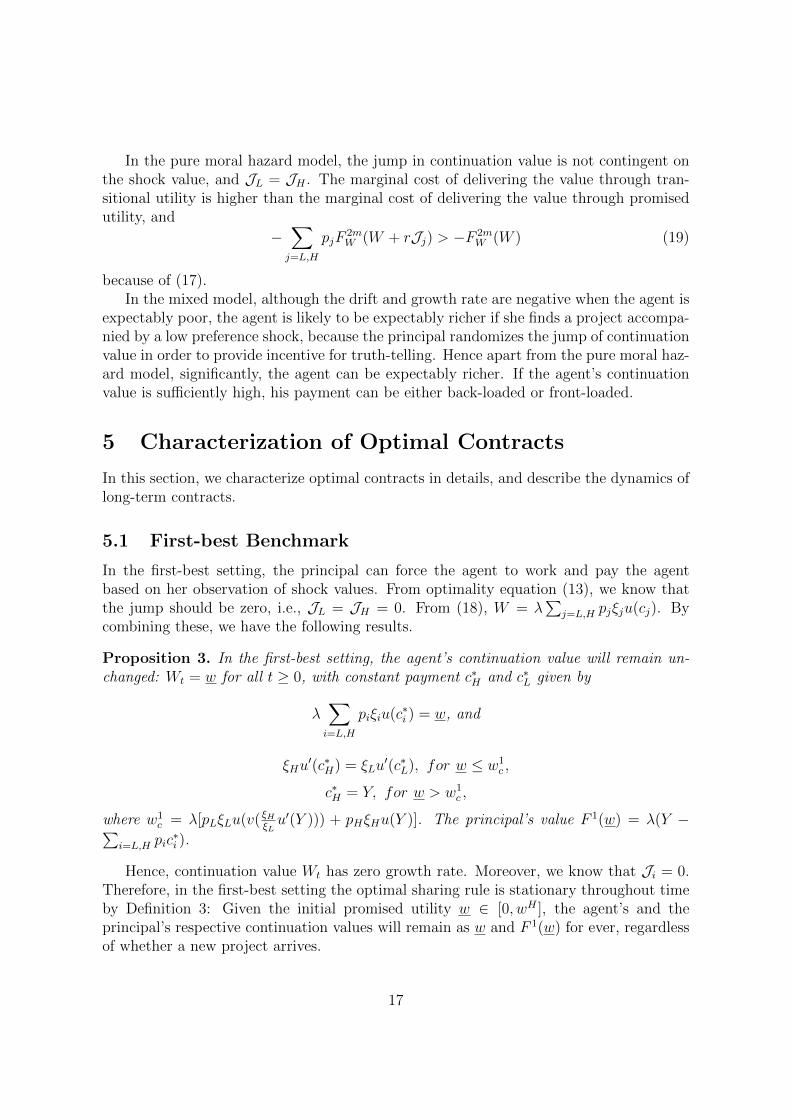
Proposition 3. In the first-best setting, the agent’s continuation value will remain un-changed: Wt = w for all t ≥ 0, with constant payment c∗H and c∗L given by
λ∑
i=L,H
piξiu(c∗i ) = w, and
ξHu′(c∗H) = ξLu
′(c∗L), for w ≤ w1c ,
c∗H = Y, for w > w1c ,
where w1c = λ[pLξLu(v( ξH
ξLu′(Y ))) + pHξHu(Y )]. The principal’s value F 1(w) = λ(Y −∑
i=L,H pic∗i ).
Hence, continuation value Wt has zero growth rate. Moreover, we know that Ji = 0.Therefore, in the first-best setting the optimal sharing rule is stationary throughout timeby Definition 3: Given the initial promised utility w ∈ [0, wH ], the agent’s and theprincipal’s respective continuation values will remain as w and F 1(w) for ever, regardlessof whether a new project arrives.
17
By the first-order condition with respect to cj on (14), 1ξju′(cj)
must be equal to
−F 1W (W ) for W < w1
c . This implies that the instantaneous payment has to be higher if theagent is expectably richer, since both cH and cL are increasing as W increases. Withoutmoral hazard or adverse selection, the payment is neither front-loaded nor back-loaded,since the drift is always equal to 0.
We measure the efficiency of the contract by defining the insurance wedge and tran-sition wedge discussed in Albanesi and Sleet (2006). The insurance wedge is computed
by ξHuc(cH)ξLuc(cL)
− 1, which measures the consumption smoothing that is implied by the opti-
mal contract. The transition wedge E[transition utilitypromised utility
]− 1 =
∑i=L.H pi
rJiW
, measures the
intertemporal smoothness of consumption. It is clear that in the first-best setting, bothwedges are equal to zero. The deviation of the wedges from zero, represents the strengthof the distortion of allocation under asymmetric information.
5.2 Pure Adverse Selection Model
0 1 2 3 40
0.5
1
1.5
2
2.5
3
3.5
4
0 1 2 3 40
1
2
0 1 2 3 40
1
2
0 1 2 3 4−1
0
1
0 1 2 4−1
0
1
W
W
W
W
W
Ww 2ac
F 2a(w )
F 1(w)
c1L
c1Hc2aH
c2aL
J2aL
J1H
J1L
J2aH
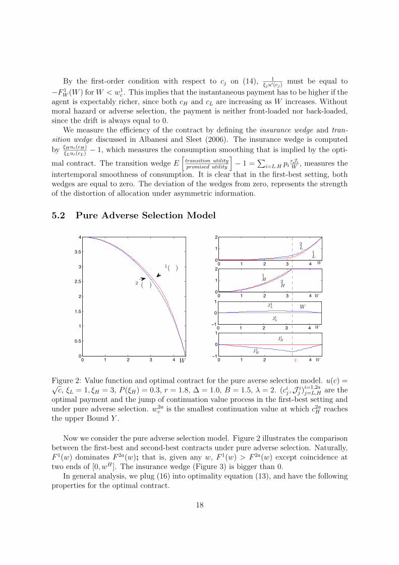
Figure 2: Value function and optimal contract for the pure averse selection model. u(c) =√c, ξL = 1, ξH = 3, P (ξH) = 0.3, r = 1.8, ∆ = 1.0, B = 1.5, λ = 2. (cij,J i
j )i=1,2aj=L,H are the
optimal payment and the jump of continuation value process in the first-best setting andunder pure adverse selection. w2a
c is the smallest continuation value at which c2aH reaches
the upper Bound Y .
Now we consider the pure adverse selection model. Figure 2 illustrates the comparisonbetween the first-best and second-best contracts under pure adverse selection. Naturally,F 1(w) dominates F 2a(w); that is, given any w, F 1(w) > F 2a(w) except coincidence attwo ends of [0, wH ]. The insurance wedge (Figure 3) is bigger than 0.
In general analysis, we plug (16) into optimality equation (13), and have the followingproperties for the optimal contract.
18
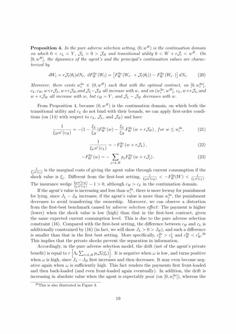
Proposition 4. In the pure adverse selection setting, (0, wH) is the continuation domainon which 0 < cL < Y , JL > 0 > JH and transitional utility 0 < W + rJi < wH . On[0, wH ], the dynamics of the agent’s and the principal’s continuation values are charac-terized by
dWt = rJt(θt)dNt, dF2aW (Wt) =
[F 2aW (Wt− + Jt(θt))− F 2a
W (Wt−)]dNt. (20)
Moreover, there exists w2ac ∈ (0, wH) such that with the optimal contract, on [0, w2a
c ],cL, cH , w+rJL, w+rJH ,and JL−JH all increase with w, and on (w2a
c , wH ], cL, w+rJL,and
w + rJH all increase with w, but cH = Y , and JL − JH decreases with w.
From Proposition 4, because (0, wH) is the continuation domain, on which both thetransitional utility and cL do not bind with their bounds, we can apply first-order condi-tions (on (14) with respect to cL, JL, and JH) and have
1
ξHu′ (cH)= −(1− ξL
ξH)F 2a
W (w)− ξLξHF 2aW (w + rJH) , for w ≤ w2a
c , (21)
1
ξLu′ (cL)= −F 2a
W (w + rJL) , (22)
−F 2aW (w) = −
∑
j=L,H
pjF2aW (w + rJj) . (23)
1ξju′(cj)
is the marginal costs of giving the agent value through current consumption if the
shock value is ξj. Different from the first-best setting, 1ξHu′(cH)
< −F 2aW (W ) < 1
ξLu′(cL).
The insurance wedge ξHu′(cH)
ξLu′(cL)− 1 > 0, although cH > cL in the continuation domain.
If the agent’s value is increasing and less than w2ac , there is more leeway for punishment
for lying, since JL − JH increases; if the agent’s value is more than w2ac , the punishment
decreases to avoid transferring the ownership. Moreover, we can observe a distortionfrom the first-best benchmark caused by adverse selection effect : The payment is higher(lower) when the shock value is low (high) than that in the first-best contract, giventhe same expected current consumption level. This is due to the pure adverse selectionconstraint (16). Compared with the first-best setting, the difference between cH and cL isadditionally constrained by (16) (in fact, we will show JL > 0 > JH), and such a differenceis smaller than that in the first best setting. More specifically, c2a
L > c1L and c2a
H < c1H .20
This implies that the private shocks prevent the separation in information.Accordingly, in the pure adverse selection model, the drift (net of the agent’s private
benefit) is equal to r[Λt
∑i=L,H piJt(ξi)
]. It is negative when ω is low, and turns positive
when ω is high, since JL−JH first increases and then decreases. It may even become neg-ative again when ω is sufficiently high. This fact renders the payments first front-loadedand then back-loaded (and even front-loaded again eventually). In addition, the drift isincreasing in absolute value when the agent is expectably poor (on [0, w2a
c ]), whereas the
20This is also illustrated in Figure 3.
19

drift is decreasing in absolute values when he becomes expectably rich (after w2ac ). When
the agent is sufficiently expectably rich, the drift may even become positive and negativeagain later.
Different from Golosov, Kocherlakota, and Tsyvinski (2003), in which consumption isfront-loaded, in pure adverse selection, as shown in Figure 3, the payment can be back-loaded when the agent is expectably poor (w < w2a
d ) and front-loaded when the agent getsexpectably richer (w > w2a
d ). Note that∑
j=L,H pjξju(cj) = ξu(cL)+pHξH(u(cH)−u(cL)).Thus, in optimum, (cH , cL) must be distorted, and u(cH)− u(cL) is smaller than that inthe first-best setting because of the adverse selection effect. Meanwhile, u(cL) has to belarger than the first-best payment for low shock. When the agent’s continuation value issmall, the adverse selection effect is strong and expected instantaneous utility is smallerthan that in the first-best setting. When the agent’s value is more than w2a
d , the paymentis front-loaded because the adverse selection effect is gradually reduced until the agent’svalue is more than w2a
c , where cH remains unchanged and the adverse selection effect isgradually reduced.
0 1 2 3 4−1
0
1
0 1 2 3 4−2
0
2
0 1 2 3 4
1
3
0 1 3 4
0
1
−1
Figure 3: Drift, growth rate and wedges for the pure adverse selection model. The dotlinein the third graph is the insurance wedge of the first-best contract. The insurance wedgeof the first-best contract is positive because cH is binding with Y when the continuationvalue is sufficiently high. w2a
d is the smallest continuation value at which the drift rate isnegative.
Finally, by Definition 3, the optimal contract is weakly stationary on continuationdomain (0, wH). The continuation value of the agent will drop (increase) if the newproject arrives accompanied by a high (low) shock. Since 0 < w + rJi < wH on CDand the growth rate is zero, Wt will remain in CD forever and will not hit 0 or wH if theagent’s initial reservation w is in CD. Then the contract will not be terminated: When theagent’s continuation value is small (< w2a
d ), the drift of the continuation value is positiveand the payment is back-loaded; this means, over the long run, that the continuation
20

value will increase. If the agent’s continuation value is sufficiently large, the drift of thecontinuation is negative and the payment is front-loaded. In the long run, the agent’scontinuation value will decrease.
5.3 Pure Moral Hazard Model
0 1 40
0.5
1
1.5
2
2.5
3
3.5
4
0 1 2 3 40
1
2
0 1 2 3 40
1
2
0 1 2 3 40
1
2
0 1 2 40
1
2
W
W
W
W
F 1(w)
F 2m(w )
c2mL
c1L
c1H
W
c2mH
J2mL
J2mH
w 2m0 w 1b w 1
cw 1b
Figure 4: Comparison of optimal contract under the first-best and the second-best settingwith pure moral hazard. u(c) =
√c, ξL = 1, ξH = 3, P (ξH) = 0.3, r = 1.8, ∆ = 1.0,
B = 1.5, λ = 2. (cij,J ij )i=1,2mj=L,H is the optimal payment and the jump in continuation value
process in the first-best and pure moral hazard models. w2m0 is the agent’s continuation
value at which the principal’s value reaches the maximum.
Now we consider the pure moral hazard model. Figure 4 illustrates the comparisonbetween optimal contracts under the first best and second best contracts with pure moralhazard. Different from Sannikov (2008) and other continuous-time moral hazard models,the agent’s payment stream directly provides incentive for the agent to work. This isbecause payment frequency is contingent on the agent’s effort, and the cost of compen-sating the agent for his effort is proportional to the cost of giving the agent value throughpromised utility. When the agent’s promised utility is low, the promised instantaneouspayment and transitional utility upon a new project’s arrival are combined to incentivizethe agent. The variance of transitional utility is minimized to be zero to reduce the prin-cipal’s risk associated with the uncertainty of preference shock, because only the mean oftransitional utility matters in the provision of incentive. If the agent’s promised utility ishigh enough, instantaneous payment can alone provide incentives, and the jump in thecontinuation value process is reduced to zero; the risk associated with the uncertainty of
21
0 1 2 3 4−1
0
1
0 1 2 3 4−10
0
10
0 1 2 40
50
1000 1 2 3 4
−2
0
2
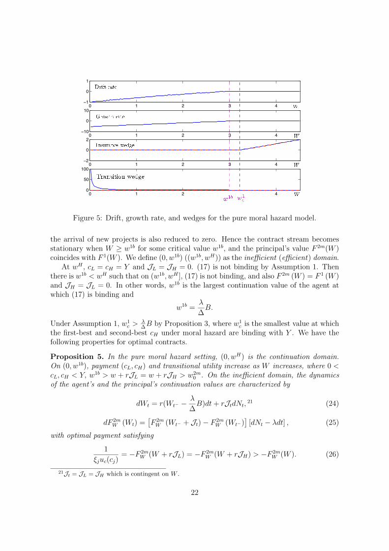
Figure 5: Drift, growth rate, and wedges for the pure moral hazard model.
the arrival of new projects is also reduced to zero. Hence the contract stream becomesstationary when W ≥ w1b for some critical value w1b, and the principal’s value F 2m(W )coincides with F 1(W ). We define (0, w1b) ((w1b, wH)) as the inefficient (efficient) domain.
At wH , cL = cH = Y and JL = JH = 0. (17) is not binding by Assumption 1. Thenthere is w1b < wH such that on (w1b, wH ], (17) is not binding, and also F 2m (W ) = F 1 (W )and JH = JL = 0. In other words, w1b is the largest continuation value of the agent atwhich (17) is binding and
w1b =λ
∆B.
Under Assumption 1, w1c >
λ∆B by Proposition 3, where w1
c is the smallest value at whichthe first-best and second-best cH under moral hazard are binding with Y . We have thefollowing properties for optimal contracts.
Proposition 5. In the pure moral hazard setting, (0, wH) is the continuation domain.On (0, w1b), payment (cL, cH) and transitional utility increase as W increases, where 0 <cL, cH < Y, w1b > w + rJL = w + rJH > w2m
0 . On the inefficient domain, the dynamicsof the agent’s and the principal’s continuation values are characterized by
dWt = r(Wt− −λ
∆B)dt+ rJtdNt,
21 (24)
dF 2mW (Wt) =
[F 2mW (Wt− + Jt)− F 2m
W (Wt−)]
[dNt − λdt] , (25)
with optimal payment satisfying
1
ξjuc(cj)= −F 2m
W (W + rJL) = −F 2mW (W + rJH) > −F 2m
W (W ). (26)
21Jt = JL = JH which is contingent on W .
22

and
JL = JH =B
∆−∑
j=L,H
pjξju (cj) , (27)
for j = L,H. On the efficient domain, the optimal contract is the same as that in thefirst best setting.
Proposition 5 states that on the inefficient domain, the payment and jump in theagent’s value must be higher than those in the first-best setting due to (17), Moreover,the moral hazard incentive compatible condition is binding only on the efficient domain.This implies that the optimal compensation and transitional utility in the first-best settingmust be distorted. More specifically, there exists a moral hazard effect: In the pure moralhazard model, the drift is negative, since r(Wt−− λ
∆B) should be negative on the inefficient
domain. This renders the payment front-loaded. But this moral hazard effect becomesweaker as w increases, since the payment and the transitional utility increase. The driftwill reduce to 0 after reaching the efficient domain. In other words, the jump in theagent’s value is gradually reduced, because the moral hazard effect decreases to zero as wincreases. On the efficient domain, there is no moral hazard effect, the payment continuesto increase, and the incentive is provided only by the agent’s instantaneous payment.
According to Proposition 5, due to the incentive compatibility condition (17), themarginal costs of giving the agent value through current consumption must be alignedwith the marginal cost of giving value through transitional utility, and JH = JL > 0if (17) is binding. Two important facts follow: First, the allocation of consumption isnot distorted across different preference shocks and the insurance wedge remains zero.However, consumption under moral hazard is improved compared to that in the first-bestsetting, and must be front-loaded. Second, as the agent’s value grows, it becomes moreexpensive to deliver the agent’s value through transitional utility, since the moral hazardeffect on the jump size of the agent’s value becomes weaker as w increases.
As illustrated by Figure 6, the agent’s value cannot jump from the inefficient domain tothe efficient domain even if there is a new project, because it is more costly to incentivizethe agent with high transitional utility if the agent is expectably rich. Moreover, undercondition (17),
r
[W − λ
∑
j=L,H
pjξju (cj)
]= r
W + λ∑
j=L,H
pjJj︸ ︷︷ ︸
expected transitional utility upon new project
−w1b
. (28)
The transitional utility gradually increases on the inefficient domain, which implies thatthe payment is front-loaded more heavily when the agent’s value is low.
On the inefficient domain, the total expected gain λ∑
j=L,H pj [ξju(cj) + Jj] has to be
w1b. Therefore, the growth rate must be negative, which is also the result of (26). Themarginal cost through transitional utility must also be larger than that through promisedutility. Then the agent’s value will decrease quickly if there is no new project, and the
23

0 1 2 41
1.5
2.5
4
4.5
Figure 6: Transitional utility.
agent may be fired if he cannot find a project for a long time. Once he finds a new project,however, his value will jump to a higher value than w2m
0 but never enter into the efficientdomain, at which first-best efficiency is achieved (see Figure 6). Hence on the one hand,even if the growth rate of the agent’s continuation value is negative, the agent is stillfully incentivized to work because his transitional utility will immediately jump to a highvalue, and he will get higher instantaneous payment once he gets a new project. On theother hand, the agent can never reach first-best efficiency if w < w1b. If w > w1b, then theagent’s continuation value will remain unchanged, and first-best efficiency is achieved.
5.4 Mixed Model with Moral Hazard and Adverse Selection
Now we consider the mixed model setting in which both moral hazard and adverse se-lection squarely exist. Figure 9 illustrates the comparison between third-best contractsunder the mixed model and the other cases. From the pure moral hazard model, weknow that if the agent’s continuation value is high enough, only instantaneous payment isrequired to provide for the agent incentive to work and the optimal contract is stationary.However, the stationary contract in the first-best setting does not satisfy the truth-tellingcondition. Hence under both moral hazard and adverse selection, optimal contracts muststill satisfy truth-telling condition (16) even if incentive compatibility condition (17) maynot be binding. Hence F 3(w) may coincide with the value function F 2a(w) of the adverseselection model if the agent is expectably rich enough (W ≥ w2b), as shown in Figure ??.That is, the third-best contract can achieve second-best efficiency with adverse selectionif the agent is expectably rich enough. Define w3
0 to be the agent’s continuation value atwhich the principal’s value reaches the maximum in the third-best contract, and w2b tobe the smallest value at which F 3(w) = F 2a(w).
We may infer that the incentive compatibility condition (17) will be binding unlessW > w2b. However, it is surprising to see that (17) is not binding, even if F 2m(W ) 6=F 3(W ). To see this, suppose that on (w1b, wH), we only consider truth-telling condition(16). From the pure adverse selection model, we know that the growth rate of the agent’s
24

0 1 3 40
0.5
1
1.5
2
2.5
3
3.5
4
0 1 2 3 40
1
2
0 1 4−1
0
1
W W
W
w 30 w 3
0w 2b
F 3(w)
F 2a(w )
C ji
J ji
w 2bw 1b
w 0b
Figure 7: Comparison of optimal contract under pure adverse selection and mixed model.u(c) =
√c, ξL = 1, ξH = 3, P (ξH) = 0.3, r = 1.8, ∆ = 1.0, B = 1.5, λ = 2. (cji ,J j
i )i=L,Hj=2a,3 isthe optimal payment and the jump of continuation value process in the third-best contractand the second-best contract with adverse selection. w3
0 is the agent’s continuation valueat which the principal’s value reaches the maximum in the third-best contract. w2b is thesmallest value at which F 3(w) = F 2a(w).
value is zero; that is, for w ∈ (w1b, wH), we have
w = λ∑
j=L,H
pj [ξju(cj) + Jj] > w1b.
This means that even on (w1b, w2b), (17) is redundant. Hence from (21)-(23),
1
ξHu′ (cH)= −(1− ξL
ξH)F 3
W (w)− ξLξHF 3W (w + rJH) , for w1b < w < w2b, (29)
1
ξLu′ (cL)= −F 3
W (w + rJL) , for w > w1b, (30)
−F 3W (w) = −
∑
j=L,H
pjF3W (w + rJj) , for w > w1b. (31)
On (0, w1b), (17) is binding, and hence the growth rate is negative. Consistent with thepure moral hazard model, we define (0, w1b) as the inefficient domain and (w1b, wH) asthe efficient domain. On the efficient domain, the allocation of consumption and incentiveprovision achieve second-best efficiency under adverse selection.
25

Proposition 6 shows that (0, wH) is the continuation domain, and we know that (17) isbinding on the inefficient domain; hence we can apply the first order condition to obtain22
1
ξHu′ (cH)= −
(1− (pH + pL
ξLξH
)
)F 3W (w + rJL)−
(pH + pL
ξLξH
)F 3W (w + rJH) ,
(32)
1
ξLu′ (cL)= −F 3
W (w + rJL) , (33)
on the inefficient domain. Hence ξHu′ (cH) > ξLu
′ (cL) and the insurance wedge is positive.Moreover, from (18), because the growth rate of the agent’s value is negative, we have
−F 3W (w) < −
∑
j=L,H
pjF3W (w + rJj) . (34)
In conclusion, we have the following result.
Proposition 6. In the mixed setting, (0, wH) is the continuation domain. On (0, w1b),payment (cL, cH) and transitional utility increase as W increases, with 0 < cL, cH < Y,W + rJL > W + rJH > w3
0. On the inefficient domain [(0, w1b)?], the dynamics of theagent’s and the principal’s continuation values are characterized by
dWt = r(Wt− −λ
∆B)dt+ rJt(θt)dNt, (35)
dF 3W (Wt) =
[F 3W (Wt− + Jt(θt))− F 3
W (Wt−)]dNt − λ
∑
j=L,H
pjJt(ξj)dt. (36)
with the optimal contract satisfying (32), (33) and (34). On the efficient domain,
dWt = rJt(θt)dNt, dF3W (Wt) =
[F 3W (Wt− + Jt(θt))− F 3
W (Wt−)]dNt. (37)
and the optimal contract satisfies (29), (30), and (31).
On the efficient domain, the moral hazard effect is removed; therefore, the optimalcontract stream can be weakly stationary. Meanwhile, on the inefficient domain, (17) isbinding and (16) holds, and we have
JL =B
∆− ξLu (cL)− pH [ξH − ξL]u (cH) or
B
∆− ξu (cH) + ξL(u(cH)− u(cL)), (38)
JH =B
∆− ξu (cH) . (39)
Hence from (32) and (33), the payment (ci)i=L,H and transitional utility increase as theagent’s value increases (Figures ?? and 11 ). On the other hand, from (38) and (39),we know that the jump decreases as the continuation value increases because the moral
22Details can be found in the proof of Proposition 6
26

0 1 3 40
0.5
1
1.5
2
2.5
3
3.5
0 1 2 3 40
0.5
1
1.5
2
0 1 2 3 4−1
−0.5
0
0.5
1
1.5
Figure 8: Comparison of optimal contract between moral hazard and mixed models.u(c) =
√c, ξL = 1, ξH = 3, P (ξH) = 0.3, r = 1.8, ∆ = 1.0, B = 1.5, λ = 2. (ci,J j
i )i=L,Hj=2m,3
is the optimal payment and the jump of continuation value process in the third-bestcontract and the second-best Contract with the moral hazard effect.
hazard effect decreases as w increases; that is, the instantaneous payment plays a largerrole in incentivizing the agent to work than the jump in the continuation value when theagent becomes expectably richer (Figure ??). Meanwhile, JL − JH = (u(cH)− u(cL)) isgradually increasing until cH = Y because the adverse selection effect becomes weaker asw increases; that is, the principal can punish the agent more for lying if he is expectablyricher. Considering the interplay between the moral hazard and adverse selection effects,the optimal payment of the agent may be front-loaded or back-loaded.
When the agent’s value is near zero, the expected instantaneous utility must be higherthan that under pure adverse selection (See Figure ?? for illustration) to incentivize theagent to work, and the payment has to be front-loaded. Moreover, we find that thepayment is front-loaded even more heavily than that under pure moral hazard, since theadverse selection effect enhances it. Note that
∑
j=L,H
pjξju(cj) = ξu(cL) + pHξH(u(cH)− u(cL)). (40)
The payment has to be distorted, and u(cH)− u(cL) is smaller in the mixed model thanthat under pure moral hazard, in order to lower the agency cost to enforce truth-telling.On the other hand, higher payment for low shock must be delivered to incentivize theagent to work.
When the agent’s value is gradually increasing, the adverse selection effect begins todominate the moral hazard effect in the sense that the payment is more heavily distortedthan the increment of the payment for the low shock (right panels in Figures ?? and 8
27
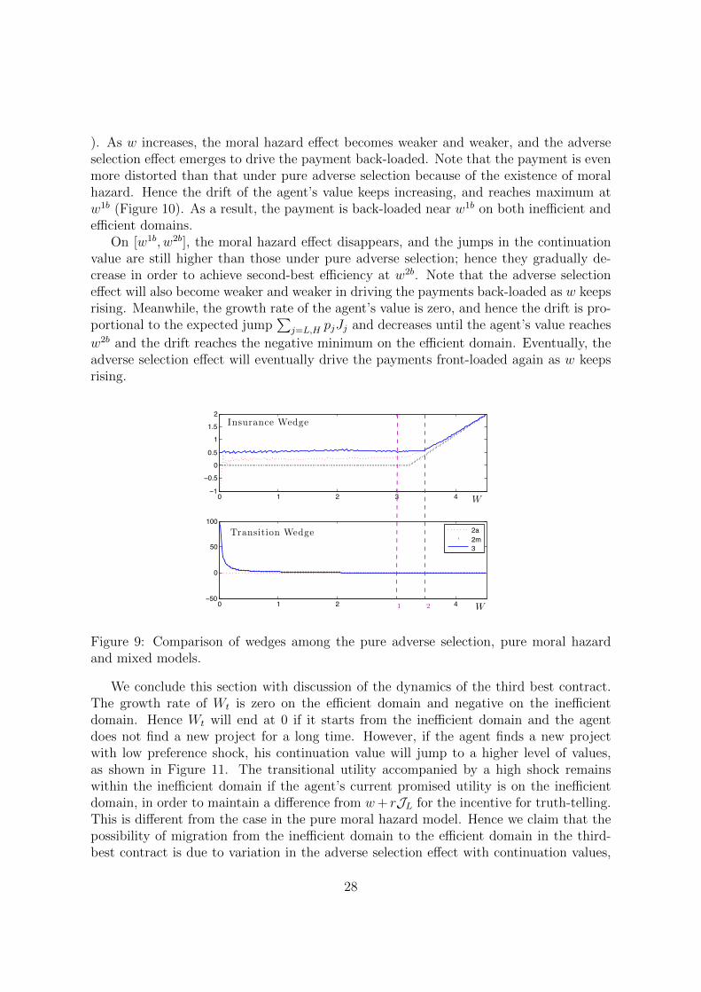
). As w increases, the moral hazard effect becomes weaker and weaker, and the adverseselection effect emerges to drive the payment back-loaded. Note that the payment is evenmore distorted than that under pure adverse selection because of the existence of moralhazard. Hence the drift of the agent’s value keeps increasing, and reaches maximum atw1b (Figure 10). As a result, the payment is back-loaded near w1b on both inefficient andefficient domains.
On [w1b, w2b], the moral hazard effect disappears, and the jumps in the continuationvalue are still higher than those under pure adverse selection; hence they gradually de-crease in order to achieve second-best efficiency at w2b. Note that the adverse selectioneffect will also become weaker and weaker in driving the payments back-loaded as w keepsrising. Meanwhile, the growth rate of the agent’s value is zero, and hence the drift is pro-portional to the expected jump
∑j=L,H pjJj and decreases until the agent’s value reaches
w2b and the drift reaches the negative minimum on the efficient domain. Eventually, theadverse selection effect will eventually drive the payments front-loaded again as w keepsrising.
0 1 2 3 4−1
−0.5
0
0.5
1
1.5
2
0 1 2 4−50
0
50
100
2a2m3
W
Insurance Wedge
Transition Wedge
Ww 2bw 1b
Figure 9: Comparison of wedges among the pure adverse selection, pure moral hazardand mixed models.
We conclude this section with discussion of the dynamics of the third best contract.The growth rate of Wt is zero on the efficient domain and negative on the inefficientdomain. Hence Wt will end at 0 if it starts from the inefficient domain and the agentdoes not find a new project for a long time. However, if the agent finds a new projectwith low preference shock, his continuation value will jump to a higher level of values,as shown in Figure 11. The transitional utility accompanied by a high shock remainswithin the inefficient domain if the agent’s current promised utility is on the inefficientdomain, in order to maintain a difference from w+ rJL for the incentive for truth-telling.This is different from the case in the pure moral hazard model. Hence we claim that thepossibility of migration from the inefficient domain to the efficient domain in the third-best contract is due to variation in the adverse selection effect with continuation values,
28

0 1 2 3 4−6
−4
−2
0
2
0 1 2 4−1.5
−1
−0.5
0
0.5
2a2m3
Growth rate
Drift rate
w 0b
w2bw1b W
W
Figure 10: Comparison of drift and growth rate of the agent’s value among three models.
for which the principal has to randomize transitional utility; also, the risk of transitionalutility upon preference shock must be larger when the agent becomes expectably richer.Finally, on the efficient domain, consumption is first back-loaded because the efficiency ofconsumption allocation is improved compared with the situation on the inefficient domain.It is then front-loaded (Figure 10), because efficiency decays as the wealth level of theagent increases, which is similar to the pattern under pure adverse selection.
6 Conclusion
This paper develops a new benchmark for investigating optimal contracts when repeatedadverse selection and dynamic moral hazard coexist. Contracts in continuous time areconveniently characterized by the agent’s continuation value. The provision of incentives,the agent’s efforts, and the revelation of the agent’s private information all depend onthe payment and the jump in the continuation value, both of which are contingent onthe agent’s reported values of preference shock. The i.i.d. assumption on private shocksis not realistic in many circumstances. However, it greatly simplifies characterization ofthe optimal contract and yields deeper insights into incentive provision under repeatedadverse selection.
The cost of compensating the agent for his effort is proportional to the costs of givingthe agent value through promised utility, and hence a prominent feature of our model isthat the efficiency of consumption allocation and incentive provision can be improved if theagent’s value is sufficiently large. The principal’s value function of the moral hazard modelcoincides with that in the first-best setting and the third-best value function coincideswith that of the pure adverse selection model in the efficient domain. The payment in thepure moral hazard model must be front-loaded to incentivize the agent to work. However,if moral hazard is mixed with adverse selection, the payment can be back-loaded becausethe adverse selection effect begins to dominate the moral hazard effect when the agent
29
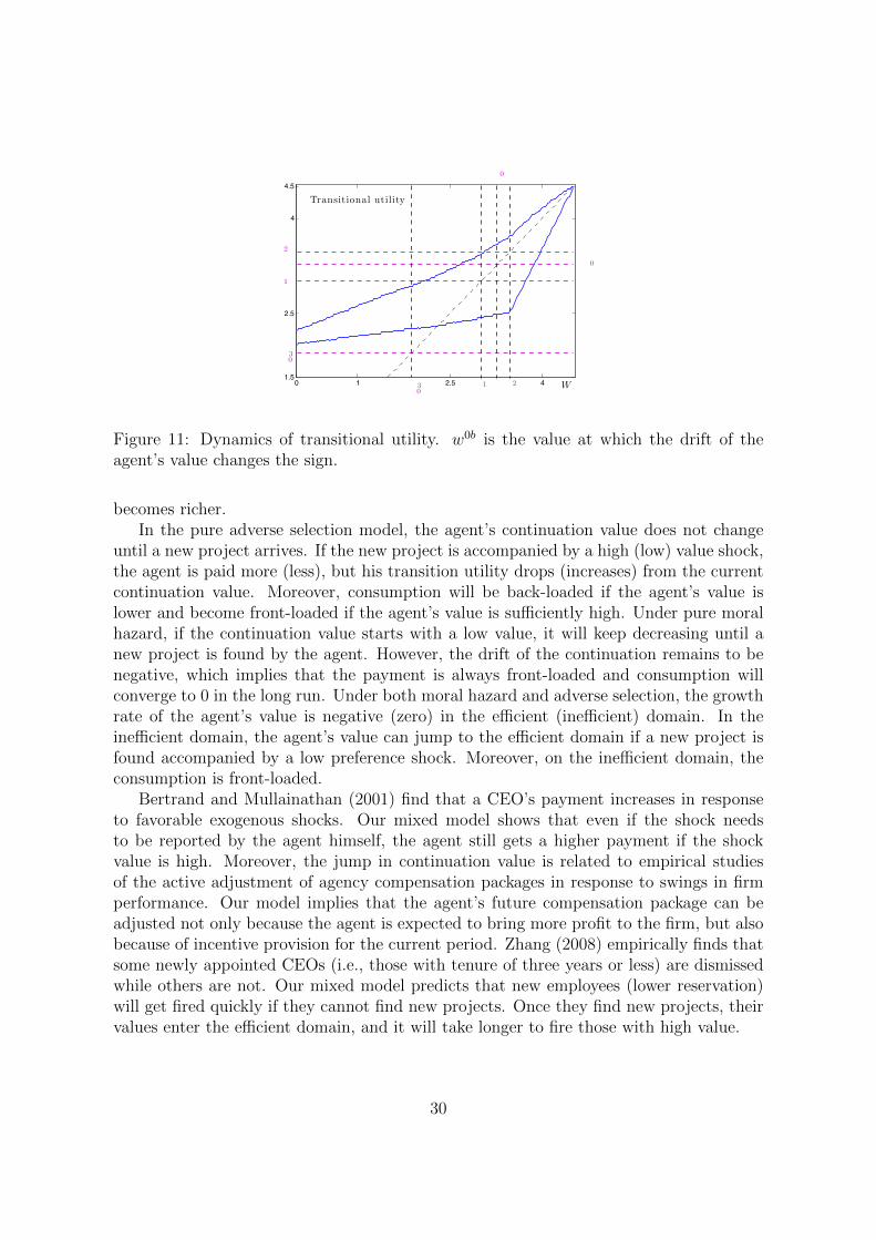
0 1 2.5 41.5
2.5
4.5
4
Ww 30
w 30
w1b
w 1b
w 2b
w 2b
w 0b
w 0b
Transitional utility
Figure 11: Dynamics of transitional utility. w0b is the value at which the drift of theagent’s value changes the sign.
becomes richer.In the pure adverse selection model, the agent’s continuation value does not change
until a new project arrives. If the new project is accompanied by a high (low) value shock,the agent is paid more (less), but his transition utility drops (increases) from the currentcontinuation value. Moreover, consumption will be back-loaded if the agent’s value islower and become front-loaded if the agent’s value is sufficiently high. Under pure moralhazard, if the continuation value starts with a low value, it will keep decreasing until anew project is found by the agent. However, the drift of the continuation remains to benegative, which implies that the payment is always front-loaded and consumption willconverge to 0 in the long run. Under both moral hazard and adverse selection, the growthrate of the agent’s value is negative (zero) in the efficient (inefficient) domain. In theinefficient domain, the agent’s value can jump to the efficient domain if a new project isfound accompanied by a low preference shock. Moreover, on the inefficient domain, theconsumption is front-loaded.
Bertrand and Mullainathan (2001) find that a CEO’s payment increases in responseto favorable exogenous shocks. Our mixed model shows that even if the shock needsto be reported by the agent himself, the agent still gets a higher payment if the shockvalue is high. Moreover, the jump in continuation value is related to empirical studiesof the active adjustment of agency compensation packages in response to swings in firmperformance. Our model implies that the agent’s future compensation package can beadjusted not only because the agent is expected to bring more profit to the firm, but alsobecause of incentive provision for the current period. Zhang (2008) empirically finds thatsome newly appointed CEOs (i.e., those with tenure of three years or less) are dismissedwhile others are not. Our mixed model predicts that new employees (lower reservation)will get fired quickly if they cannot find new projects. Once they find new projects, theirvalues enter the efficient domain, and it will take longer to fire those with high value.
30

References
[1] Albanesi, S., & Armenter, R. (2012). Intertemporal distortions in the second best.Review of Economic Studies, 79(4), 1271-1307.
[2] Albanesi, S., & Sleet, C. (2006). Dynamic optimal taxation with private information.Review of Economic Studies, 73(1), 1-30.
[3] Allen, F. (1983). Credit rationing and payment incentives. Review of Economic Stud-ies, 50(4), 639-646.
[4] Armstrong, M., & Vickers, J. (2010). A model of delegated project choice. Econo-metrica, 78(1), 213-244.
[5] Atkeson, A., & Lucas Jr, R. E. (1992). On efficient distribution with private infor-mation. Review of Economic Studies, 59(3), 427-453.
[6] Bernardo, A. E., Cai, H., & Luo, J. (2001). Capital budgeting and compensation withasymmetric information and moral hazard. Journal of Financial Economics, 61(3),311-344.
[7] Bertrand, M., & Mullainathan, S. (2001). Are CEOs rewarded for luck? The oneswithout principals are. Quarterly Journal of Economics, 116(3), 901-932.
[8] Biais, B., Mariotti, T., Rochet, J. C., & Villeneuve, S. (2010). Large risks, limitedliability, and dynamic moral hazard. Econometrica, 78(1), 73-118.
[9] Bolton, P., & Dewatripont, M. (2005). Contract theory. MIT press.
[10] Chassang, S. (2013). Calibrated incentive contracts. Econometrica, 81(5), 1935-1971.
[11] Cvitanic, J., & Zhang, J. (2007). Optimal compensation with adverse selection anddynamic actions. Mathematics and Financial Economics, 1(1), 21-55.
[12] DeMarzo, P. M., & Sannikov, Y. (2006). Optimal Security Design and DynamicCapital Structure in a Continuous-Time Agency Model. Journal of Finance, 61(6),2681-2724.
[13] Fernandes, A., & Phelan, C. (2000). A recursive formulation for repeated agencywith history dependence. Journal of Economic Theory, 91(2), 223-247.
[14] Garleanu, N., & Pedersen, L. H. (2003). Adverse selection and the required return.Review of Financial Studies, 17(3), 643-665.
[15] Green, E.J. (1987). Lending and the smoothing of uninsurable income. In E.C.Prescott and N. Wallace (eds.), Contractual Arrangement for Intertemporal Trade,3-25. Minneapolis: University of Minnesota Press.
31

[16] Golosov, M., Kocherlakota, N., & Tsyvinski, A. (2003). Optimal indirect and capitaltaxation. Review of Economic Studies, 70(3), 569-587.
[17] Harris, M., Kriebel, C. H., & Raviv, A. (1982). Asymmetric information, incentivesand intrafirm resource allocation. Management Science, 28(6), 604-620.
[18] Harris, M., & Raviv, A. (1996). The capital budgeting process: Incentives and infor-mation. The Journal of Finance, 51(4), 1139-1174.
[19] Hart, O. (2009). Hold-up, asset ownership, and reference points. Quarterly Journalof Economics, 124(1), 267-300.
[20] He, Z. (2008). Optimal executive compensation when firm size follows geometricbrownian motion. Review of Financial Studies, 22(2), 859-892.
[21] Hoffmann, F., & Pfeil, S. (2010). Reward for luck in a dynamic agency model. Reviewof Financial Studies, 23(9), 3329-3345.
[22] Holmstrom, B., & Tirole, J. (1997). Financial intermediation, loanable funds, andthe real sector. Quarterly Journal of Economics, 112(3), 663-691.
[23] Jacod, J. and Shiryaev, A.N. (2003). Limit theorems for stochastic processes. Berlin,Springer-Verlag, second edition.
[24] Jenter, D., & Kanaan, F. (2015). CEO turnover and relative performance evaluation.Journal of Finance, 70(5), 2155-2184.
[25] Jewitt, I., Kadan, O., & Swinkels, J. M. (2008). Moral hazard with bounded pay-ments. Journal of Economic Theory, 143(1), 59-82.
[26] Kloyer, M. and Helm, R. (2008). Contractual design of contract R&D: State-of-the-Art of Empirical Research. Technology and Innovation Management, 151-165.
[27] Kocherlakota, N. R. (2010). The new dynamic public finance. Princeton UniversityPress.
[28] Lewis, T. R. (2012). A theory of delegated search for the best alternative. RANDJournal of Economics, 43(3), 391-416.
[29] Last, F. and Brandt A. (2003). Marked point processes on the real line: the dynamicapproach. New York: Springer-Verlag.
[30] Li, R. (2011). Dynamic agency with persistent exogenous shocks. Working paper,University of Wisconsin# Madison.
[31] Malenko, A. (2011). Optimal design of internal capital markets. Working Paper,Massachusetts Institute of Technology.
32

[32] Mason, R., & Valimaki, J. (2015). Getting it done: dynamic incentives to completea project. Journal of the European Economic Association, 13(1), 62-97.
[33] Mirrlees, J. A. (1971). An exploration in the theory of optimum income taxation.Review of Economic Studies, 38(2), 175-208.
[34] Øksendal, B. K. and Sulem, A. (2010). Applied stochastic control of jumpdiffusions,”Springer-Verlag, 2nd Edition.
[35] Ramsey, F. P. (1928). A mathematical theory of saving. Economic Journal, 38(152),543-559.
[36] Rogerson, W. P. (1985). Repeated moral hazard. Econometrica, 69-76.
[37] Sadzik, T., & Stacchetti, E. (2015). Agency models with frequent actions. Economet-rica, 83(1), 193-237.
[38] Sannikov, Y. (2007a). Agency problems, screening and increasing credit lines. Work-ing Paper.
[39] Sannikov, Y. (2007b). Games with imperfectly observable actions in continuous time.Econometrica, 75(5), 1285-1329.
[40] Sannikov, Y. (2008). A continuous-time version of the principal-agent problem. Re-view of Economic Studies, 75(3), 957-984.
[41] Sannikov, Y., & Skrzypacz, A. (2010). The role of information in repeated gameswith frequent actions. Econometrica, 78(3), 847-882.
[42] Stiglitz, J. E., & Weiss, A. (1983). Incentive effects of terminations: Applications tothe credit and labor markets. American Economic Review, 73(5), 912-927.
[43] Stulz, R. (1990). Managerial discretion and optimal financing policies. Journal offinancial Economics, 26(1), 3-27.
[44] Sung, J. (2005). Optimal contracts under adverse selection and moral hazard: acontinuous-time approach. Review of Financial Studies, 18(3), 1021-1073.
[45] Tchistyi, A. (2005). Security design with correlated hidden cash flows: The optimalityof performance pricing. Working Paper.
[46] Thomas, J., & Worrall, T. (1990). Income fluctuation and asymmetric information:An example of a repeated principal-agent problem. Journal of Economic Theory,51(2), 367-390.
[47] Townsend, R. M. (1982). Optimal multiperiod contracts and the gain from enduringrelationships under private information. Journal of political Economy, 90(6), 1166-1186.
33
[48] Ulbricht, R. (2016). Optimal delegated search with adverse selection and moral haz-ard. Theoretical Economics, 11(1), 253-278.
[49] Vath, V. L., Pham, H., & Villeneuve, S. (2008). A mixed singular/switching con-trol problem for a dividend policy with reversible technology investment. Annals ofApplied Probability, 18(3), 1164-1200.
[50] Williams, N. (2011). Persistent private information. Econometrica, 79(4), 1233-1275.
[51] Williams, N. (2015). A solvable continuous time dynamic principal–agent model.Journal of Economic Theory, 159, 989-1015.
[52] Zhang, Y. (2008). Information asymmetry and the dismissal of newly appointedCEOs: An empirical investigation. Strategic Management Journal, 29(8), 859-872.
[53] Zhang, Y. (2009). Dynamic contracting with persistent shocks. Journal of EconomicTheory, 144(2), 635-675.
[54] Zhu, J. Y. (2012). Optimal contracts with shirking. Review of Economic Studies,80(2), 812-839.
34

Appendix
A Proof of Lemma 1
Define the gain process Gt by
e−rtGt := E
{∫ ∞
0
re−rsθsu (cs(θs)) dNs +
∫ ∞
0
re−rs1[Λs=λ−∆]Bds|ht− , θt},
and e−rtGt is a martingale. On one side, by the definition of the continuation value, wehave
e−rtGt = e−rtWt +
∫ t
0
re−rsθsu (cs(θs)) dNs +
∫ t
0
re−rs1[Λs=λ−∆]Bds.
On the other side, by the martingale representation theorem for a marked point process(Last and Brandt 2003[29]) , there exists a predictable γt (θt) and
de−rtGt = re−rtγt(θt)dNt − re−rtΛt
∑
i=L,H
piγt(ξi)dt.
Define Jt(θt) = γt(θt) − θtu (ct (θt)), and applying Ito’s formula we obtain the represen-
tation form of Wt. Moreover, Nt = r∫ t
0Js(θs)dNs − r
∫ t0
{Λs
∑i=L,H piJs(ξi)
}ds is a
martingale.
B Proof of Proposition 1
It has been proved in the main text that (7), (8), and (9) necessarily hold if (GIC) is true.We only need to prove the sufficiency. Consider an arbitrary reporting strategy σ and
effort Λt. Define e−rtGt =∫ t
0re−rsθsu
(cs
(θs
))dNs+
∫ t0re−rs1[Λs=λ−∆]Bds+e−rtWt with
W0 := w, where Wt is the continuation value process contingent on the agent’s report anddesirable effort {Λt}t≥0. Note that
e−rtGt = w+e−rtKt+
∫ t
0
re−rs (θsu(cs(θs)) + Js(θs)) dNs−∫ t
0
re−rsλs∑
i=L,H
(ξiu(cs(ξi)) + Js(ξi)) ds
where
e−rtKt :=
∫ t
0
re−rs{[
1[Λs=λ−∆]B − 1[Λs=λ−∆]B]−[Λs − Λs
] ∑
i=L,H
(ξiu(cs(ξi)) + Js(ξi))}ds
+
∫ t
0
re−rs[θsu(cs
(θs
))+ Js(θs)− θsu (cs (θs))− Js(θs)
]dNs
35

The first and second parts of the integration of e−rtKt are negative because of (7), (8),and (9). Hence, e−rtGt is a supermartingale. Note that {ct} are bounded from below,hence e−rtGt is a supermartingale bounded from below. Hence, we add
∫ ∞
0
re−rsθsu(cs(θs)
)dNs +
∫ ∞
0
re−rs1[Λs=λ−∆]Bds
as the last element of the supermartingale e−rtGt by the martingale convergence theorem(Last and Brandt 2003[29]). Therefore,
w = G0 ≥ E
[∫ ∞
0
re−rsθsu(cs(θs)
)dNs +
∫ ∞
0
re−rs1[Λs=λ−∆]Bds
].
Hence, the truth-telling strategy σ∗ with {Λt}t≥0 is at least as good as any alternative
strategy σ with effort plan{
Λt
}t≥0
.
C Proof of Proposition 2
We prove that F 2a(W ) is strictly concave and monotone, and Υ3(W ) = Υ2a(W )∩Υ2m(W ).Other parts can be derived similarly.
C.1 F 2a(W ) is concave and monotone
Given two initial values w1, w2 ∈ [0, wH ], w1 > w2 of the agent’s continuation valueprocesses, we need to prove
F 2a (wχ) > χF 2a (w1) + (1− χ)F 2a (w2) .
where wχ = χw1 + (1− χ)w2, where 0 < χ < 1.We assume that (J i
t (θt), cit(θt))i=1,2 is the optimal incentive compatible contract for
the agent with initial value wi and
dW it = rW i
t−dt+ rJ it (θt)dNt − rλ
∑
j=L,H
pj{ξju(cit(ξj)) + J i
t (ξj)}dt,W i
0 = wi.
Under pure adverse selection,(cjt(ξj),J j
t (ξj))j=L,H
satisfy (7), (8), 0 ≤ W it + rJ i
t (ξj) ≤wH . Under pure adverse selection, high effort can be dictated. If W i
t hits 0, thenciv (θj) = J i
v (ξj) = 0, for v ≥ t. If W it hits wH , civ (θj) = Y, J i
v (ξj) = 0 for v ≥ t. Weconstruct W 3
t with (c3t (ξj),J 3
t (ξj)) satisfying
dW 3t = rW 3
t−dt+ rJ 3t (θt)dNt − rλ
∑
j=L,H
pj{ξju(c3
t (ξj)) + J 3t (ξj)
}dt,W i
0 = wχ
where c3t (θt) is defined by
u(c3t (θt)
)= χu
(c1t (θt)
)+ (1− χ)u
(c2t (θt)
).
36

Then, c3t (θt) ≤ χc1
t (θt) + (1− χ) c2t (θt). Moreover, the equality holds only when
c1t (θt) = c2
t (θt), because u(c) is strictly concave. Also, let J 3t (ξj) = χJ 1
t (ξj)+(1− χ)J 2t (ξj).
Hence (c3t (ξj),J 3
t (ξj)) satisfy (7), (8) and 0 ≤ W it + rJ 3
t (ξj) ≤ wH . W 3t = χW 1
t +(1− χ)W 2
t . Then, from the definition of the value function F 2a(w), we know thatF 2a (wχ) ≥ χF 2a (w1) + (1− χ)F 2a (w2). Moreover, the equality holds only when c1
t (θ) =c2t (θ) because u(c) is strictly concave, which implies the strict concavity of F 2a(W ).
For monotonicity, let 0 < w1 < w2 < wH ; we define W 2t as previously, and we let
c1t (θt) = c2
t (θt) ,J 1t (θt) = J 2
t (θt). Hence W 1t < W 2
t , before W 1t or W 2
t hits 0 or wH .Moreover, we know that F 2a(w) ∈ [F 2a(wH), F 2a(0)] . So W 1
t will hit wH earlier than W 2t ,
and we have monotonicity for F 2a(w).
C.2 Υ3(W ) = Υ2a(W ) ∩Υ2m(W )
Next, we want to prove Υ3(W ) = Υ2a(W ) ∩Υ2m(W ), which is to prove
JL = JH + ξL [u(cH)− u(cL)] (41)
under the constraint ∆∑
j=L,H pj [ξju(cj) + Jj] ≥ B. Obviously, from (7) and (8), wehave cH ≥ cL at optimality. If cH = cL, by (7) and (8), then (41) holds. Suppose cH > cL.We only need to show ξL [u(cH)− u(cL)] ≤ JL − JH must be binding at optimality.Suppose not; then at w, the optimal (ci,Ji) satisfies
ξL [u(cH)− u(cL)] < JL − JH . (42)
Thus, we have W + rJL > 0; otherwise, W + rJH < 0. With sufficiently small δ, defineJ δL = JL − δ,J δ
H = JH + pLpHδ. We still have ξL [u(cH)− u(cL)] < J δ
L − J δH , and
∆∑
j=L,H pj[ξju(cj) + J δ
j
]= ∆
∑j=L,H pj [ξju(cj) + Jj] ≥ B. The optimality of (cj,Jj)
implies that there exists no δ > 0, which makes the right-hand side of (13) larger givencH and cL. It implies
F 3W
(W + rJ δ
H
)− F 3
W
(W + rJ δ
L
)|δ=0 ≤ 0.
With the assumption of strict concavity, we have JH ≥ JL, which contradicts (42) andcH > cL. Then, (41) holds.
D Proof of Proposition 4
Plugging in the corresponding constraints shown by Proposition 2 on [0, wH ], the dynamicsof the agent’s and the principal’s continuation values are given as in Proposition 4.
D.1 F 2aW (0) = 0, F 2a
W
(wH)≤ − 1
ξu′(Y ).
On the RHS of optimality equation (13), we take a pooling payment cL = cH = b andJi = 0. Then we have
[F 2a (W )−WF 2a
W (W )]≥ max
0≤b≤Yλ [Y − b]− λF 2a
W (W ) ξu (b) . (43)
37

Suppose F 2aW (0+) 6= 0. By Proposition 2, F 2a
W (0+) < 0. Let W ↘ 0+, from (43) we have
0 ≥ max0≤b≤Y
−b− F 2aW
(0+)ξu (b) . (44)
Note that with b′ = 0, −b′ − F 2aW (0) ξu (b′) = 0. Given F 2a
W (0+) < 0, there exists b∗ > 0such that −b∗−F 2a
W (0) ξu (b∗) > 0, which contradicts (44). Hence we prove F 2aW (0+) = 0.
On the other hand, if we let W ↗ wH in (43), then we have
wHF 2aW
(wH)≤ min
bλ [b− Y ] + λF 2a
W
(wH)ξu (b) .
When b′ = Y ,wHF 2a
W
(wH)
= λ [b′ − Y ] + λF 2aW
(wH)ξu (b′) .
Hence, Y achieves the minimum for 0 ≤ b ≤ Y . Then we have 1 + F 2aW
(wH)θu′ (Y ) ≤ 0,
that is,
F 2aW
(wH)≤ − 1
ξu′ (Y ).
D.2 r[W − λξu (cH)
]+ λ [W − TH ] = 0.
IC constraint (16) can be transformed into
TL = TH + rξL(u(cH)− u(cL)), u(cH) ≥ u(cL) (45)
where Ti = W + rJi is the transitional problem. (13) can be transformed into
(r + λ)F 2a (W )− (r + λ)F 2aW (W )W = max
C∈Υi(W )rλ
[Y −
∑
j=L,H
pjcj
]− rλF 2a
W (W )∑
j=L,H
pjξju (cj)
(46)
+ λ
( ∑
j=L,H
pj(F 2a (Tj)− F 2a
W (W )Tj)).
At W = 0, the optimal contract is Tj = cj = 0 because FW (0) = 0. At W = wH , Tj = wH
and cj = Y can be verified as the optimal solution. Denote uj = u (cj) and U (.) as theinverse function of u (.) , which is convex and increasing. Denote uH = δ + uL We plug(45) into (43) and (46) becomes
(r + λ)F 2a (W )− (r + λ)F 2aW (W )W (47)
= maxuL,TH ,δ
rλ [Y − pHU (uL + δ)− pLU (uL)]− λF 2aW (W )
[TH + rξuL + rξδ
]
+ λ(pLF
2a (TH + rξLδ) + pHF2a (TH)
),
subject toTH ≥ 0, TH + rξLδ ≤ wH , δ ≥ 0,uL ≥ 0, δ + uL ≤ u (Y ) .
38

−rpHU (uL + δ)− rpLU (uL) +pLF2a (TH + rξLδ) +pHF
2a (TH) are jointly concave on(uL, TH , δ) , −λF 2a
W (W ) increases as W increases; hence optimal (uL, TH , δ) increase giventhat TH + rξLδ < wH and δ + uL < u (Y ), which means that (uL, uH , TL, TH) increase asW increases. Applying envelope theorem on (47) we have
r[W − λξu (cH)
]+ λ [W − TH ] = 0 (48)
The reason we can apply envelope theorem without Lagrange multipliers is that theconditions of all the control variables in (47) are not dependent on the state variable W .Note that (48) implies that the growth rate is zero for all W .
D.3 The optimal contract is not pooling on(0, wH
)
Suppose pooling contract c∗H = c∗L = c∗ is optimal at W ∗ ∈(0, wH
). We have T ∗L = T ∗H =
W ∗. Since the growth rate is proved to be zero in the last step, we have W ∗ = λξu (c∗). Because 0 < W ∗ < wH , 0 < c∗ < Y . From the optimality of pooling payment at W ∗,we can derive two facts. First, given T ∗H = W ∗, c∗L = c∗, we define u (cH) = u (c∗ + δ) andTL = T ∗H+rξL [u (c∗ + δ)− u (c∗)], δ ≥ 0. With sufficiently small δ > 0, 0 < u (cH) < u(Y )and 0 < TL < wH . Then optimality of the pooling contract implies that the optimal valuefor δ is 0. Plug (T ∗H , TL, c∗L, cH) into optimality equation (13), and RHS is reduced to
maxδ≥0−rpH (c∗ + δ)− rF 2a
W (W ) ξu (c∗ + δ) + pLF2a (W ∗ + rξL [u (c∗ + δ)− u (c∗)])
If δ = 0 is optimal, taking the first order condition with respect to δ and taking value 0for δ, we have
−1− ξHF 2aW (W ∗)u′ (c∗) ≤ 0 (49)
The second fact is given the pooling payment is optimal, we have
−1− ξF 2aW (W ∗)u′(c∗) = 0; (50)
because 0 < c∗ < Y . Then (50) contradicts (49), because ξH > ξ and F 2aW (W ∗) < 0.
Hence, cH is not pooling with cL. From our proof, it is clear that the strict monotonicityof the value function is a crucial condition for the non-pooling payment.
D.4 The optimal payment with low preference shock is not zeroon(0, wH
)
Suppose c∗L = 0, hence c∗H 6= 0 because on(0, wH
)the optimal contract is not pooling.
ThenrξL [u (c∗H)− u (c∗L)] = T ∗L − T ∗H < rξH [u (c∗H)− u (c∗L)]
We keep T ∗L , T ∗H and improve c∗L by small amount such that
rξL [u (c∗H)− u (c∗L + δ)] < T ∗L − T ∗H < rξH [u (c∗H)− u (c∗L + δ)] .
Sufficiently small δ > 0 makes the RHS of (47) larger, because F 2aW (W ∗) < 0 on (0, wH)
and contradicts c∗L = 0.
39
D.5 0 < T ∗H < W < T ∗L < wH for W ∈(0, wH
)
First prove T ∗L 6= wH and T ∗H 6= 0. If at w∗ ∈ (0, wH), the optimal T ∗L = wH , then from(47), the principal can always be better off by lowering δ unless δ = 0. However if δ = 0,the optimal payment at w∗ is pooling, which contradicts D.3.
Suppose that at some w∗ ∈ (0, wH), the optimal T ∗H = 0. From (47) we know that u∗L,δ∗ and T ∗H are increasing as W increases before u∗L + δ reaches u (Y ) (we just show thaton (0, wH), T ∗L < wH ). After u∗L + δ∗ reaches u (Y ), we can see that T ∗H , T ∗L , c∗L continuesto increase and δ∗ decreases. From D.2, we know that at w∗ = 0, c∗H = c∗L = 0 and T ∗H =T ∗L = 0. Hence for any w∗ ∈
(0, wH
), T ∗H > 0. Then at any w∗ ∈
(0, wH
), the optimal
transition utility 0 < T ∗i < wH . Hence(0, wH
)is the continuation domain. Because the
growth rate is zero, we have∑
i piFw∗(T ∗i ) = FW (w∗) from (18) and TH < w∗ < TL.Plugging in the corresponding constraints shown by Proposition 2, the dynamics of
the agent’s and the principal’s continuation values are given as in Proposition 5.On (0, w1b), RHS of (13) is reduced to
maxci,Ti−rλ
∑
j=L,H
pju (cj) + λ∑
j=L,H
pjF2m (Tj)
subject to
∆∑
j=L,H
pj [rξju (cj) + Tj] ≥ rB + ∆W. (51)
where Tj is the transitional utility for j = L,H. The monotonicity of contracts is obviousand
(0, wH
)is the continuation domain, which can be investigated in detail by applying
the method of Proposition 4 and the fact that F 2m(w) = F 1(w) if w > w1b.Then on(0, w1b
)there exists Lagrange multiplier δ (w) > 0 contingent on w,
−λF 2mW (Tj) = δ (w) , rλ = rδ (w) ξjuc (cj) .
Hence TH = TL := T , ξjuc (cj) = − 1F 2mW (T )
. Then F 2mW (T ) < 0 and T ≥ w2m
0 . Moreover,
by the monotonicity of the optimal contract, on (0, w1b),∑
j=L,H pjξju (cj) increases to B∆
and {Tj}j=L,H increase to w1b.Finally, on the inefficient domain, (51) is binding. Hence the growth rate is negative
and (19) holds true from (18), and we have (26).
E Proof of Proposition 6
Plugging in the corresponding constraints shown by Proposition 2, the dynamics of theagent’s and the principal’s continuation values are given as in Proposition 6.
40

The maximization problem on RHS of (13) can be reduced to
maxC∈Υi(W )
− rλ∑
j=L,H
pjcj] + rF 3W (W )
(W − λ
∑
j=L,H
pjξju (cj)
)(52)
+ λ
( ∑
j=L,H
pj(F 3 (Tj)− rF 3
W (W )Tj)),
subject to (51) and
TL = TH + rξL(u(cH)− u(cL)), u(cH) ≥ u(cL). (53)
Then the proof of the monotonicity of (ci, Ti) is similar to that of Proposition 4. If w islarge enough, F 3(w) = F 2a(w). Then TL < wH , cL < Y if w < wH and hence (0, wH) isthe continuation domain.
When w > w1b we can ignore condition (51), because with only (53), the growth rateof W is zero by Proposition 4. Then λ
∑j=L,H pj [ξju (cj) + Jj] = w > w1b = λ
∆B. Note
that for w ∈ [w1b, w2b), only (53) holds, although F 3(w) < F 2a(w). On (0, w1b), RHS of(52) is reduced to
maxci,Ti−rλ
∑
j=L,H
pju (ci) + λ∑
j=L,H
pjF3 (Tj)
subject to ∆∑
j=L,H pj [rξju (cj) + Tj] ≥ rB + ∆W and (53). Thus, on(0, w1b
)there
exists a Lagrange multiplier δ (W ) > 0 contingent on w, and then the problem is reducedto
maxuL,κ,TH
−r [pLU (uL) + pHU (uL + κ)] + rξδ (W ) [uL + κ]
+ pLF3 (TH + rξLκ) + pHF
3 (TH) + δ (W ) TH ,
where U is the inverse function of u and uj = u (cj), κ = u(cH) − u(cL). Note thatw1b < w2m
c < w3c ; hence 0 < cL, cH < Y and 0 < TL, TH < wH . First-order conditions
yield
pL1
u′ (cL)= −ξLpLF 3
W (TL) ,
pH1
u′ (cH)= ξδ (W ) + ξLpLF
3W (TL) ,
δ (W )=−pLF 3W (TL)− pHF 3
W (TH) .
Hence
1
ξHu′ (cH)= −
(pL − pL
ξLξH
)F 3W (TL)−
(pH + pL
ξLξH
)F 3W (TH) ,
1
ξLu′ (cL)= −F 3
W (TL) .
41

Graz Economics PapersFor full list see:
http://ideas.repec.org/s/grz/wpaper.html
Address: Department of Economics, University of Graz,
Universitatsstraße 15/F4, A-8010 Graz
11–2018 Xi Chen, Yu Chen and Xuhu Wan: Delegated Project Search
10–2018 Stefan Nabernegg, Birgit Bednar-Friedl, Pablo Munoz, Michaela Titz and
Johanna Vogel: National policies for global emission reductions: Effectiveness of
carbon emission reductions in international supply chains
09–2018 Jonas Dovern and Hans Manner: Order Invariant Tests for Proper Calibration
of Multivariate Density Forecasts
08–2018 Ioannis Kyriakou, Parastoo Mousavi, Jens Perch Nielsen and Michael
Scholz: Choice of Benchmark When Forecasting Long-term Stock Returns
07–2018 Joern Kleinert: Globalization Effects on the Distribution of Income
06–2018 Nian Yang, Jun Yang and Yu Chen: Contracting in a Continuous-Time Model
with Three-Sided Moral Hazard and Cost Synergies
05–2018 Christoph Kuzmics and Daniel Rodenburger: A case of evolutionary stable
attainable equilibrium in the lab
04–2018 Robert J. Hill, Alicia N. Rambaldi, and Michael Scholz: Higher Frequency
Hedonic Property Price Indices: A State Space Approach
03–2018 Reza Hajargasht, Robert J. Hill, D. S. Prasada Rao, and Sriram Shankar:
Spatial Chaining in International Comparisons of Prices and Real Incomes

02–2018 Christoph Zwick: On the origin of current account deficits in the Euro area
periphery: A DSGE perspective
01–2018 Michael Greinecker and Christopher Kah: Pairwise stable matching in large
economies
15–2017 Florian Brugger and Jorn Kleinert: The strong increase of Austrian government
debt in the Kreisky era: Austro-Keynesianism or just stubborn forecast errors?
14–2017 Jakob Mayer, Gabriel Bachner and Karl W. Steininger: Macroeconomic
implications of switching to process-emission-free iron and steel production in Europe
13–2017 Andreas Darmann, Julia Grundner and Christian Klamler: Consensus in the
2015 Provincial Parliament Election in Styria, Austria: Voting Rules,Outcomes, and
the Condorcet Paradox
12–2017 Robert J. Hill, Miriam Steurer and Sofie R. Waltl: Owner Occupied Housing
in the CPI and Its Impact On Monetary Policy During Housing Booms and Busts
11–2017 Philipp Kohlgruber and Christoph Kuzmics: The distribution of article quality
and inefficiencies in the market for scientific journals
10–2017 Maximilian Goedl: The Sovereign-Bank Interaction in the Eurozone Crisis
09–2017 Florian Herold and Christoph Kuzmics: The evolution of taking roles
08–2017 Evangelos V. Dioikitopoulos, Stephen J. Turnovsky and Ronald Wendner:
Dynamic Status Effects, Savings, and Income Inequality
07–2017 Bo Chen, Yu Chen and David Rietzke: Simple Contracts under Observable and
Hidden Actions
06–2017 Stefan Borsky, Andrea Leiter and Michael Paffermayr: Product Quality and
Sustainability: The Effect of International Environmental Agreements on Bilateral
Trade
05–2017 Yadira Mori Clement and Birgit Bednar-Friedl: Do Clean Development
Mechanism projects generate local employment? Testing for sectoral effects across
Brazilian municipalities
04–2017 Stefan Borsky, Alexej Parchomenko: Identifying Phosphorus Hot Spots: A
spatial analysis of the phosphorus balance as a result of manure application
03–2017 Yu Chen, Yu Wang, Bonwoo Koo: Open Source and Competition Strategy
Under Network Effects
02–2017 Florian Brugger: The Effect of Foreign and Domestic Demand on U.S. Treasury
Yields
01–2017 Yu Chen: On the Equivalence of Bilateral and Collective Mechanism Design
13–2016 Jan de Haan, Rens Hendriks, Michael Scholz: A Comparison of Weighted
Time-Product Dummy and Time Dummy Hedonic Indexes
12–2016 Katja Kalkschmied: Complementary Institutional Elements and Economic
Outcomes
11–2016 Dieter Balkenborg, Josef Hofbauer, Christoph Kuzmics: The refined best
reply correspondence and backward induction
10–2016 Karl W. Steininger, Wolf D. Grossmann, Iris Grossmann: The economic
value of dispatchable solar electricity: a Post-Paris evaluation
09–2016 Sofie R. Waltl: Estimating aggregate quantile-specific gross rental yields for
residential housing in Sydney
08–2016 Karl Farmer: Financial integration and house price dynamics in equilibrium
modeling of intra-EMU and global trade imbalances
07–2016 Gabriel Bachner, Birgit Bednar-Friedl: Counterbalancing the Effects of Climate
Change Adaptation on Public Budgets: Factor Taxes, Transfers, or Foreign Lending?
06–2016 Margareta Kreimer, Ricardo Mora: Segregated Integration: Recent Trends in
the Austrian Gender Division of Labor
05–2016 Karl Farmer, Bogdan Mihaiescu: Credit constraints and differential growth in
equilibrium modeling of EMU and global trade imbalances

04–2016 Daniel Eckert, Frederik Herzberg: The birth of social choice theory from the
spirit of mathematical logic: Arrow’s theorem in the framework of model theory
03–2016 Christoph Kuzmics, Jan-Henrik Steg: On public good provision mechanisms
with dominant strategies and balanced budget
02–2016 Florian Gauer, Christoph Kuzmics: Cognitive Empathy in Conflict Situations
01–2016 Thomas Aronsson, Olof Johansson-Stenman, Ronald Wendner:
Redistribution Through Charity, and Optimal Taxation when People are Concerned
with Social Status
09–2015 Sofie R. Waltl: Variation across price segments and locations: A comprehensive
quantile regression analysis of the Sydney housing market
08–2015 Karl Farmer, Bogdan Mihaiescu: Pension systems and financial constraints in a
three-country OLG model of intra-EMU and global trade imbalances
07–2015 Javier Lopez Prol, Karl W. Steininger: Photovoltaic self-consumption
regulation in Spain: profitability analysis and alternative regulation schemes.
06–2015 Miriam Steurer, Caroline Bayr: Quantifying Urban Sprawl using Land Use Data
05–2015 Porfirio Guevara, Robert J. Hill, Michael Scholz: Hedonic Indexes for Public
and Private Housing in Costa Rica
04–2015 Sofie R. Waltl: A Hedonic House Price Index in Continuous Time
03–2015 Ronald Wendner: Do Positional Preferences for Wealth and Consumption Cause
Inter-Temporal Distortions?
02–2015 Maximilian Godl, Christoph Zwick: Stochastic Stability of Public Debt: The
Case of Austria
01–2015 Gabriel Bachner: Land Transport Systems under Climate Change: A
Macroeconomic Assessment of Adaptation Measures for the Case of Austria