getting started with rhrv version 2.0 - r...
TRANSCRIPT

Getting started with RHRVVersion 2.0
Constantino A. Garcıa∗, Abraham Otero, Xose Vila, Arturo Mendez,
Leandro Rodrıguez-Linares and Marıa Jose Lado

January 31, 2014
ii


Acknowledgements
We would like to thank Matias Garcia-Constantino for his kind contributions and
suggestions.
iv

Contents
Acknowledgements . . . . . . . . . . . . . . . . . . . . . . . . . . . . . . . iv
List of Tables . . . . . . . . . . . . . . . . . . . . . . . . . . . . . . . . . . x
List of Figures . . . . . . . . . . . . . . . . . . . . . . . . . . . . . . . . . . xi
1 Overview 4
1.1 Aim . . . . . . . . . . . . . . . . . . . . . . . . . . . . . . . . . . . . 7
1.2 Structure of the document . . . . . . . . . . . . . . . . . . . . . . . . 7
2 Heart Rate Variability 9
2.1 Obtaining HRV time series . . . . . . . . . . . . . . . . . . . . . . . . 13
2.1.1 QRS detection . . . . . . . . . . . . . . . . . . . . . . . . . . 13
2.1.2 Constructing HRV time series . . . . . . . . . . . . . . . . . . 16
2.1.3 Preprocessing HRV time series . . . . . . . . . . . . . . . . . . 17
2.2 HRV analysis techniques . . . . . . . . . . . . . . . . . . . . . . . . . 18
2.2.1 Time domain methods . . . . . . . . . . . . . . . . . . . . . . 18
2.2.2 Frequency domain methods . . . . . . . . . . . . . . . . . . . 21
2.2.3 Nonlinear Methods . . . . . . . . . . . . . . . . . . . . . . . . 25
v

CONTENTS
2.2.3.1 Phase space reconstruction . . . . . . . . . . . . . . 25
2.2.3.2 Correlation dimension . . . . . . . . . . . . . . . . . 27
2.2.3.3 Generalized correlation dimension . . . . . . . . . . . 28
2.2.3.4 Information dimension . . . . . . . . . . . . . . . . . 29
2.2.3.5 Sample entropy . . . . . . . . . . . . . . . . . . . . . 29
2.2.3.6 Maximum Lyapunov exponent . . . . . . . . . . . . 30
2.2.3.7 Detrended Fluctuation Analysis (DFA) . . . . . . . . 31
2.2.3.8 Recurrence Quantification Analysis (RQA) . . . . . . 32
2.2.3.9 Poincare plot . . . . . . . . . . . . . . . . . . . . . . 32
2.3 HRV alterations related to specific pathologies . . . . . . . . . . . . . 34
3 Installation 38
3.1 Installation . . . . . . . . . . . . . . . . . . . . . . . . . . . . . . . . 38
3.2 WFDB applications . . . . . . . . . . . . . . . . . . . . . . . . . . . . 39
3.3 Troubleshooting . . . . . . . . . . . . . . . . . . . . . . . . . . . . . . 40
3.3.1 tkrplot dependency . . . . . . . . . . . . . . . . . . . . . . . . 40
4 A 15-minutes guide to RHRV 41
4.1 Preprocessing the Heart Rate series . . . . . . . . . . . . . . . . . . . 43
4.1.1 Load heart beat positions . . . . . . . . . . . . . . . . . . . . 43
4.1.2 Calculating HR and filtering . . . . . . . . . . . . . . . . . . . 45
4.1.3 Interpolating . . . . . . . . . . . . . . . . . . . . . . . . . . . 46
4.1.4 Plotting . . . . . . . . . . . . . . . . . . . . . . . . . . . . . . 47
4.2 Analyzing the Heart Rate series . . . . . . . . . . . . . . . . . . . . . 47
vi

CONTENTS
4.2.1 Accessing “raw data” . . . . . . . . . . . . . . . . . . . . . . . 47
4.2.2 Time-domain analysis techniques . . . . . . . . . . . . . . . . 49
4.2.3 Frequency-domain analysis techniques . . . . . . . . . . . . . 53
4.2.3.1 Fourier . . . . . . . . . . . . . . . . . . . . . . . . . 54
4.2.3.2 Wavelets . . . . . . . . . . . . . . . . . . . . . . . . 56
4.2.3.3 Creating several analyses . . . . . . . . . . . . . . . 59
4.2.3.4 Plotting . . . . . . . . . . . . . . . . . . . . . . . . . 61
4.2.3.5 A brief comparison: wavelets Vs. Fourier . . . . . . . 62
5 Some more advanced features of RHRV 65
5.1 Completing our first tour . . . . . . . . . . . . . . . . . . . . . . . . . 65
5.1.1 Creating the structure . . . . . . . . . . . . . . . . . . . . . . 66
5.1.2 Reading heart beats . . . . . . . . . . . . . . . . . . . . . . . 67
5.1.3 Constructing the time series . . . . . . . . . . . . . . . . . . . 68
5.1.4 Filtering the time series . . . . . . . . . . . . . . . . . . . . . 69
5.1.5 Interpolation . . . . . . . . . . . . . . . . . . . . . . . . . . . 72
5.1.6 Time analysis . . . . . . . . . . . . . . . . . . . . . . . . . . . 72
5.1.7 Frequency analysis . . . . . . . . . . . . . . . . . . . . . . . . 73
5.2 Reading several file formats . . . . . . . . . . . . . . . . . . . . . . . 77
5.2.1 Reading RR files . . . . . . . . . . . . . . . . . . . . . . . . . 77
5.2.2 Reading files in WFDB format . . . . . . . . . . . . . . . . . . 77
5.2.3 Other formats . . . . . . . . . . . . . . . . . . . . . . . . . . . 79
5.2.4 A general function . . . . . . . . . . . . . . . . . . . . . . . . 79
5.3 Performing analysis in different intervals of a recording . . . . . . . . 81
vii

CONTENTS
5.3.1 AddEpisodes . . . . . . . . . . . . . . . . . . . . . . . . . . . 81
5.3.2 Plotting episodic information . . . . . . . . . . . . . . . . . . 83
5.3.3 LoadEpisodesAscii . . . . . . . . . . . . . . . . . . . . . . . . 85
5.3.4 LoadApneaWFDB . . . . . . . . . . . . . . . . . . . . . . . . 88
5.3.5 Analyzing HRV inside and outside the episodes . . . . . . . . 90
5.4 Storing and reading HRVData . . . . . . . . . . . . . . . . . . . . . . 95
6 HRV nonlinear analysis 97
6.1 An introduction to nonlinear analysis techniques . . . . . . . . . . . . 97
6.1.1 Nonlinearity Test . . . . . . . . . . . . . . . . . . . . . . . . . 99
6.1.2 Phase space reconstruction . . . . . . . . . . . . . . . . . . . . 103
6.1.2.1 Time lag estimation . . . . . . . . . . . . . . . . . . 103
6.1.2.2 Embedding dimension estimation . . . . . . . . . . . 107
6.1.3 Computing nonlinear statistics . . . . . . . . . . . . . . . . . . 109
6.1.3.1 The classic correlation dimension . . . . . . . . . . . 109
6.1.3.2 Sample entropy . . . . . . . . . . . . . . . . . . . . . 115
6.1.3.3 Maximum Lyapunov exponent . . . . . . . . . . . . 119
6.1.3.4 Detrended Fluctuation Analysis . . . . . . . . . . . . 123
6.1.3.5 Recurrence Quantification Analysis . . . . . . . . . . 127
6.2 Advanced nonlinear analysis techniques . . . . . . . . . . . . . . . . . 131
6.2.1 Nonlinear noise reduction . . . . . . . . . . . . . . . . . . . . 134
6.2.2 Generalized correlation dimensions . . . . . . . . . . . . . . . 135
6.2.3 Information dimension . . . . . . . . . . . . . . . . . . . . . . 136
6.2.4 Poincare Plot . . . . . . . . . . . . . . . . . . . . . . . . . . . 141
viii

CONTENTS
Bibliography 146
ix
List of Tables
2.1 Summary of the most broadly used nonlinear statistics. . . . . . . . . 26
2.2 Most important RQA statistics. . . . . . . . . . . . . . . . . . . . . 33
2.3 Clinical value of HRV analysis in cardiological diseases . . . . . . . . 35
5.1 LoadBeat operation depending on the fileType parameter. . . . . . . . 80
x
List of Figures
2.1 Modulation of the heart rate by the ANS . . . . . . . . . . . . . . . . 10
2.2 Heart rate variation . . . . . . . . . . . . . . . . . . . . . . . . . . . . 11
2.3 Influence of the ANS system over the different HRV frequency bands. 14
2.4 Normal electrocardiogram. . . . . . . . . . . . . . . . . . . . . . . . . 15
2.5 High and low frequencies illustrated with sines. . . . . . . . . . . . . 22
2.6 Two wavelets . . . . . . . . . . . . . . . . . . . . . . . . . . . . . . . 24
4.1 Non interpolated Heart Rate time plot example. . . . . . . . . . . . . 48
4.2 Interpolated Heart Rate time plot example. . . . . . . . . . . . . . . 49
4.3 The most important fields stored in the HRVData structure. . . . . . 50
4.4 Plot obtained with the PlotPowerBand for the Fourier-based analysis. 62
4.5 Plot obtained with the PlotPowerBand for the wavelet-based analysis. 63
5.1 All the fields stored in the HRVData structure. . . . . . . . . . . . . 66
5.2 Modifying default values in the FilterNIHR function . . . . . . . . . . 70
5.3 Manually removal of artifacts with EditNIHR. . . . . . . . . . . . . . 71
5.4 Plot obtained with the PlotSpectrogram function. . . . . . . . . . . . 75
xi

LIST OF FIGURES
5.5 PlotSpectrogram using the freqRange parameter . . . . . . . . . . . . 76
5.6 Episodic information in the Non interpolated Heart Rate time series. 84
5.7 Episodic information in the interpolated Heart Rate time series. . . . 85
5.8 Episodic information in all the power bands. . . . . . . . . . . . . . . 86
5.9 Loading Apnea episodes using the LoadApneaWFDB function. . . . . 91
6.1 Surrogate data testing. . . . . . . . . . . . . . . . . . . . . . . . . . . 102
6.2 Calculation of the optimum time lag using the autocorrelation . . . . 106
6.3 Estimation of the embedding dimension using the Cao’s algorithm. . 108
6.4 Correlation sums calculation. . . . . . . . . . . . . . . . . . . . . . . 112
6.5 . . . . . . . . . . . . . . . . . . . . . . . . . . . . . . . . . . . . . . . 114
6.6 Sample entropy computations. . . . . . . . . . . . . . . . . . . . . . . 117
6.7 Sample entropy estimation. . . . . . . . . . . . . . . . . . . . . . . . 119
6.8 Divergence computations for the maximum Lyapunov exponent. . . . 122
6.9 Maximum Lyapunov exponent estimation. . . . . . . . . . . . . . . . 123
6.10 DFA. . . . . . . . . . . . . . . . . . . . . . . . . . . . . . . . . . . . . 126
6.11 Recurrence plot. . . . . . . . . . . . . . . . . . . . . . . . . . . . . . . 129
6.12 Recurrence plot. . . . . . . . . . . . . . . . . . . . . . . . . . . . . . . 130
6.13 Autocorrelation function for the RR time series. . . . . . . . . . . . 132
6.14 Automatic estimation of the embedding dimension. . . . . . . . . . . 133
6.15 Generalized correlation dimension computations. . . . . . . . . . . . . 137
6.16 Generalized correlation dimension estimation. . . . . . . . . . . . . . 138
6.17 Information dimension computations in RHRV. . . . . . . . . . . . . 140
6.18 Information dimension estimation. . . . . . . . . . . . . . . . . . . . . 141
xii

LIST OF FIGURES
6.19 “Classic” Poincare Plot. . . . . . . . . . . . . . . . . . . . . . . . . . . 143
6.20 Poincare Plot using the confidence region estimation. . . . . . . . . . 145
xiii

Acronyms
ANS Autonomic Nervous System.
bpm Beats Per Minute.
DFT Discrete Fourier Transform.
ECG electrocardiogram.
FFT Fast Fourier Transform.
HF High Frequency.
HR Heart Rate.
HRV Heart Rate Variability.
IRRR length of the interval determined by the first and the third quantile of the
∆RR time series.
LF Low Frequency.
1

Acronyms
MADRR Median of the Absolute values of the successive Differences between the
RR intervals.
MODWPT Maximal Overlap Discrete Wavelet Packet Transform.
niHR Non Interpolated Heart Rate.
pNN50 proportion of successive RR intervals greater than 50 ms.
PSD Power Spectrum Density.
RMSSD Root Mean Square of Successive Differences.
RSA Respiratory Sinus Arrhythmia.
SA sinoatrial node.
SDANN Standard Deviation of the Average NN/(RR) intervals calculated over
short periods.
SDNN Standard Deviation of the NN interval.
SDNN index the mean of the standard deviation calculated over the windowed RR
intervals.
SDSD Standard Deviation of Successive Differences.
STFT Short Time Fourier Transform.
TINN Triangular Interpolation of NN (RR) interval histogram.
2

Acronyms
ULF Ultra Low Frequency.
VLF Very Low Frequency.
3

Chapter 1
Overview
It has been recognized in the past two decades that there is a significant relation-
ship between the Autonomic Nervous System (ANS) and cardiovascular mortality,
including sudden cardiac death. Experimental evidence for a connection between a
propensity for cardiac failure and either increased sympathetic or reduced parasym-
pathetic activity has encouraged the search of quantitative markers of autonomic
activity.
One of the most promising non-invasive markers is Heart Rate Variability (HRV).
HRV refers to the variation over time of both the intervals between consecutive
heart beats and the instantaneous Heart Rate (HR). As the heart rhythm is mod-
ulated by the ANS, HRV is thought to reflect the activity of the sympathetic and
parasympathetic branches of the ANS. The continuous modulation of the ANS
results in continuous variations in heart rate. HRV has been recognized to be a
4

useful non-invasive tool as a predictor of several pathologies such as myocardial in-
farction, diabetic neuropathy, sudden cardiac death and ischemia, among others [17].
The existence of several software tools (Kubios HRV [32], the HRV toolkit for
MatLab [24] or aHRV [27], just to mention a few) have helped to popularize its use.
Some of these software packages are commercial and require the purchase of expen-
sive licenses (e.g., aHRV). Even although others are free, they require the purchase
of expensive commercial software on which they depend (e.g., the HRV toolkit for
MatLab). Kubios is free (though not open source), but it is based on a graphical
user interface, which makes it extremely tedious to perform systematic analyses of
a large database of recordings, as the user must manually load and analyze through
the user interface each recording. In this context, we have developed RHRV, an
open-source package for the statistical environment R [12], [13], [30], [34]. To the
best of our knowledge, RHRV is the only completely free and open source software
package for performing HRV analysis and that is based on scripting commands; thus
it enables the easy automation of analyses of a large number of recordings.
RHRV provides a complete set of tools for HRV analysis which can be used for devel-
oping new HRV analysis algorithms or for performing clinical experiments. Although
this software is mainly designed for the analysis of the HRV in humans, it may also
be used by animal researchers. Among the main characteristics of RHRV, we may
highlight:
5
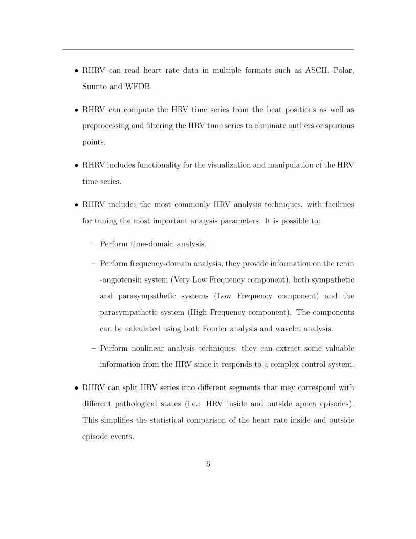
• RHRV can read heart rate data in multiple formats such as ASCII, Polar,
Suunto and WFDB.
• RHRV can compute the HRV time series from the beat positions as well as
preprocessing and filtering the HRV time series to eliminate outliers or spurious
points.
• RHRV includes functionality for the visualization and manipulation of the HRV
time series.
• RHRV includes the most commonly HRV analysis techniques, with facilities
for tuning the most important analysis parameters. It is possible to:
– Perform time-domain analysis.
– Perform frequency-domain analysis; they provide information on the renin
-angiotensin system (Very Low Frequency component), both sympathetic
and parasympathetic systems (Low Frequency component) and the
parasympathetic system (High Frequency component). The components
can be calculated using both Fourier analysis and wavelet analysis.
– Perform nonlinear analysis techniques; they can extract some valuable
information from the HRV since it responds to a complex control system.
• RHRV can split HRV series into different segments that may correspond with
different pathological states (i.e.: HRV inside and outside apnea episodes).
This simplifies the statistical comparison of the heart rate inside and outside
episode events.
6

1.1. AIM
• RHRV provides flexibility for accessing directly the internal data structures
that it uses in its calculations.
The RHRV package can be freely downloaded from the R-CRAN repository [2].
1.1 Aim
The aim of this tutorial is to help the user to get started with the RHRV package for
the R environment. This document supposes that the user has some basic knowledge
about both the R environment and HRV. However, a short introduction to HRV will
be given, and further references are provided.
1.2 Structure of the document
The remainder of this document is structured as follows. First, a brief review of
several HRV topics is given in Chapter 2. This chapter contains a short discussion on
the physiological origins of heart rate variability, as well as a review of the frequency
components of HRV. Section 2.1 continues discussing the extraction of heart beat
periods. The derivation and the preprocessing of HRV time series are also described.
In Section 2.2, the most common HRV analysis methods are summarized (although
they will be covered in more depth when they are introduced in the document). The
descriptions of the methods are divided into time-domain, frequency-domain, and
nonlinear. A discussion on the important issue of stationarity is included. The rest
of the chapter (Section 2.3) is focused on the use of HRV as a predictor of different
7

1.2. STRUCTURE OF THE DOCUMENT
pathologies and its clinical applications.
Chapter 3 explains how to get RHRV installed in your computer. This guide assumes
that you have already installed R in your computer.
Chapter 4 presents a “15-minutes guide to RHRV”. This chapter presents the es-
sential functions needed to perform basic time and frequency domain analysis with
RHRV. Chapter 5 completes the functionality introduced in Chapter 4 and presents
more advanced features available in RHRV focusing on reading RR intervals stored
in different formats and episodic information analysis.
Chapter 6 introduces the functionality needed to perform HRV nonlinear analysis
with RHRV.
8
Chapter 2
Heart Rate Variability
Heart Rate Variability (HRV) describes variations over time of both instantaneous
HR and the intervals between consecutive heart beats. The rhythm of the heart is
modulated by the sinoatrial node (SA), which is largely influenced by both the sym-
pathetic and parasympathetic branches of the ANS (see Figure 2.1). Sympathetic
activity increases the heart rate and its response is slow (a few seconds). On the
other hand the parasympathetic activity decreases the heart rate and its response is
faster (0.2-0.6 seconds). Parasympathetic influence on heart rate is mediated by the
action of the vagus nerve. There are also some feedback mechanisms modulating the
heart rates, that try to maintain cardiovascular homeostasis by responding to the
perturbations sensed by baroreceptors and chemoreceptors.
9

Figure 2.1: Modulation of the heart by the sympathetic and parasympathetic systems.Figure taken from [1].
10

Under resting conditions, vagal tone prevails. However, parasympathetic and sym-
pathetic activity constantly interact. The continuous modulation of the ANS results
in continuous variations in heart rate as shown in Figure 2.2. The beat to beat inter-
val variations are the result of the interaction of the beat-to-beat control mechanisms.
time
voltage
Figure 2.2: Heart rate variation as a consequence of the modulation of the ANS.
Due to the different speed of response of both branches of the ANS, it is possible to
use the frequency analysis to discriminate between the sympathetic and parasym-
pathetic contributions to the HRV. Akselrod et al. [4] described three components
in the HRV power spectrum with physiological relevance: the Very Low Frequency
(VLF) component (frequencies below 0.03 Hz), the Low Frequency (LF) component
(0.03-0.15 Hz) and the High Frequency (HF) component (0.15-0.4 Hz). However, at
present there is no absolute consensus on the precise limits of their boundaries.
Among all the HF mechanisms involved in the heart rate modulation we find the so
called Respiratory Sinus Arrhythmia (RSA): the heartbeat synchronization with the
respiratory rhythm [7]. In addition to the breathing frequencies, the HF component
is believed to be of parasympathetic origin. It should be noted that, although it is
11
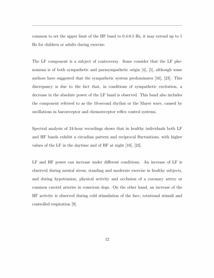
common to set the upper limit of the HF band to 0.4-0.5 Hz, it may extend up to 1
Hz for children or adults during exercise.
The LF component is a subject of controversy. Some consider that the LF phe-
nomena is of both sympathetic and parasympathetic origin [4], [5], although some
authors have suggested that the sympathetic system predominates [16], [23]. This
discrepancy is due to the fact that, in conditions of sympathetic excitation, a
decrease in the absolute power of the LF band is observed. This band also includes
the component referred to as the 10-second rhythm or the Mayer wave, caused by
oscillations in baroreceptor and chemoreceptor reflex control systems.
Spectral analysis of 24-hour recordings shows that in healthy individuals both LF
and HF bands exhibit a circadian pattern and reciprocal fluctuations, with higher
values of the LF in the daytime and of HF at night [10], [23].
LF and HF power can increase under different conditions. An increase of LF is
observed during mental stress, standing and moderate exercise in healthy subjects,
and during hypotension, physical activity and occlusion of a coronary artery or
common carotid arteries in conscious dogs. On the other hand, an increase of the
HF activity is observed during cold stimulation of the face, rotational stimuli and
controlled respiration [9].
12
2.1. OBTAINING HRV TIME SERIES
The LF/HF ratio is often used by some investigators [9] as a quantitative mirror
of the sympatho/vagal balance. However, other researchers disagree about the
usefulness of the LF/HF index [7].
Finally, the rhythms associated with VLF have not been studied as deeply as the
higher frequencies. Indeed, some authors doubt that there is a specific physiological
process attributable to these heart period changes. Furthermore, the VLF band is
affected by algorithms of baseline removal [9]. Despite all these objections, some
authors have related the Very Low Frequency with the renin-angiotensin system.
Finally, it is possible to split this band into another two: the Very Low Frequency
Band (VLF, 0.003-0.03 Hz) and the Ultra Low Frequency (ULF) Band(0-0.003 Hz).
Unless explicitly mentioned, the VLF band will be used to refer the (0 - 0.03 Hz)
band.
Figure 2.3 summarizes the influence of the ANS system over the different HRV
frequency bands.
2.1 Obtaining HRV time series
2.1.1 QRS detection
The aim of HRV analysis is to analyze the sinus rhythms while it is modulated by
the ANS. Thus, the starting point for HRV analysis should be the extraction of
13

2.1. OBTAINING HRV TIME SERIES
HF: (0.15-0.4) HzParasympathetic origin
LF: (0.03-0.15) HzParasympathetic andsympathetic origin
VLF: (<0.03) Hzrenin-angiotensin system
Figure 2.3: Influence of the ANS system over the different HRV frequency bands.
the SA-node action potentials from the electrocardiogram (ECG). A typical ECG
showing a heartbeat consists of a P wave, a QRS complex and a T wave (see Figure
2.4). The P wave represents the wave of depolarization that spreads from the
SA-node throughout the atria. The QRS complex reflects the rapid depolarization
of the right and left ventricles. Since the ventricles are the largest part of the heart,
in terms of mass, the QRS complex usually has a much larger amplitude than the
P-wave. The T wave represents the ventricular repolarization of the ventricles. On
rare occasions, a U wave can be seen following the T wave. The U wave is believed
to be related to the last remnants of ventricular repolarization.
14

2.1. OBTAINING HRV TIME SERIES
P
Q
R
S
TST
SegmentPRSegment
PR Interval
QT Interval
QRS Complex
Figure 2.4: Normal electrocardiogram.
The observable that is closest related to the action of the SA-node is the P wave and,
thus, the heartbeat period is defined as the time difference between two different P
waves. However, the signal to noise ratio (SNR) of the P wave is smaller than the
QRS complex SNR. Therefore, the QRS complexes are more easily detected than
the P waves and, for convenience, the heart beat period is computed as the time
difference between two successive QRS complexes. For the sake of simplicity, we
will not discuss the QRS detectors in this tutorial. Further information about QRS
detection may be found in [20].
15

2.1. OBTAINING HRV TIME SERIES
2.1.2 Constructing HRV time series
After the QRS complex occurrences have been detected, the HRV time series
(sometimes called the RR time series) may be calculated. The intervals between
consecutive heart beats needed to construct the time series are called RR intervals,
inter-beat intervals or interval function. In some context, normal-to-normal intervals
(NN) may also be used when referring to these intervals.
RR intervals are computed as the difference between successive R-wave occurrence
times tn. That is, the n-th RR interval RRn will be computed as
RRn = α · (tn − tn−1), (2.1)
where α is a conversion parameter that may vary depending of the units in which
the RR time series will be expressed. Usually, the RR intervals are expressed in ms
and thus, if the occurrence times are expressed in seconds, α is setted as α = 1000.
It must be noticed that, in some studies, the HRV is constructed as the sequence of
the instantaneous heart rates. That is
HRn =β
tn − tn−1
. (2.2)
Again, β is used as a conversion parameter. Since the HR is usually expressed in
Beats Per Minute (bpm), β = 60 if the occurrence times are expressed in seconds.
In this section, for the sake of simplicity, the RRn construction will be used.
16

2.1. OBTAINING HRV TIME SERIES
The resulting RR series will consist of a set of pairs (tn, RRn). It should be noted
that this time series is not equidistantly sampled (that is why the time value, tn, must
be specified). This must be taken into account before frequency-domain analysis,
since it requires an uniformly sampled time series. There are several approaches to
overcome this issue [9]. RHRV uses interpolation for transforming the non-uniformly
sampled RR series into an equidistantly sampled one. After interpolation, regular
frequency analysis may be applied. A second approach, maybe the simplest one,
assumes equidistant sampling and constructs a signal, called tachogram, using RR
intervals as a function of a beat number. However, when using this approach, the
spectrum is not a function of the frequency, rather of cycles per beat. A third
approach receives the name of the spectrum of the counts, that is, it uses a series of
impulses (delta functions) positioned at beat occurrence times. This approach relies
on the commonly accepted Integral Pulse Frequency Modulator (IPFM) model [6],
[15], that simulates the modulation of the sinoatrial node.
2.1.3 Preprocessing HRV time series
Before performing the analysis of any RR time series, a filtering operation must be
carried out in order to eliminate outliers or spurious points present in the signal with
unacceptable physiological values. Outliers present in the series originate from the
detection of an artifact as a heartbeat (RR interval too short), or from the loss of a
heartbeat in the detection procedure (RR interval too large). The RR time series
may also contain some physiological artifacts. Physiological artifacts include ectopic
17

2.2. HRV ANALYSIS TECHNIQUES
beats (an ectopic beat occurs when the heart beat is not triggered by the SA-node,
causing an “extra” beat) and arrhythmic events. If detection of the heartbeat has
been revised and corrected manually by a physician, this step can be skipped.
2.2 HRV analysis techniques
The purpose of analysis techniques usually is to extract useful physiological informa-
tion that may help researchers to create new disease markers or predictors. There
are several tools to perform HRV analysis, however these are usually classified into
three categories: time domain methods, frequency domain methods and non-linear
methods. A brief review of the main techniques of time domain, frequency domain
and nonlinear methods is presented. Further information may be found at [9].
2.2.1 Time domain methods
The simplest HRV analysis techniques are the time domain measures. Since there
exist a wide variety of time domain techniques, we will focus on those included in
the RHRV software.
The best known time analysis statistic may be the standard deviation of the RR
interval: Standard Deviation of the NN interval (SDNN).
SDNN =
√√√√ 1
N − 1
N∑j=1
(RRj −RR)2
18

2.2. HRV ANALYSIS TECHNIQUES
Since the variance is mathematically equal to the total power of spectral analysis,
SDNN reflects the power of the components responsible for variability. The SDNN
reflects both short-term and long-term variations within the RR series. However, it
should be noted that total variance of HRV increases with the length of the analyzed
recording [31]. Thus, on arbitrarily ECGs, SDNN may not be an appropriate HRV
analysis variable because of its dependence with the recording’s length. To avoid
this issue, statistical variables calculated from segments of the total monitoring
period may be used. Among this type of variables are the SDANN, the standard
deviation of the average NN (RR) intervals calculated over short periods (usually 5
minutes); and the SDNN index, the mean of the standard deviation calculated over
the windowed RR intervals, usually 5 minutes.
Other measures use the time series constructed as successive RR interval differences,
defined as
∆RRj = RRj+1 −RRj.
The Standard Deviation of Successive Differences (SDSD) is given by
SDSD =
√√√√ 1
N − 1
N∑j=1
(∆RRj −∆RR)2.
The Root Mean Square of Successive Differences (RMSSD) is given by
RMSSD =
√√√√ 1
N − 1
N∑j=1
(∆RRj)2.
19

2.2. HRV ANALYSIS TECHNIQUES
Other measures using the successive RR interval differences include the length of
the interval determined by the first and the third quantile of the ∆RR time series
(IRRR); and the median of the absolute values of the ∆RR time series (MADRR,
Median of the Absolute Differences of the RR intervals).
Other commonly used measures derived from interval differences include NN50, the
number of interval differences of successive RR intervals greater than 50 ms, and
pNN50, the proportion derived by dividing NN50 by the total number of RR intervals.
All these measures derived from interval differences estimate the HF variation in
heart rhythm and thus, they are highly correlated.
Finally, in addition to these statistical parameters, there are some geometric mea-
sures that can be calculated from the RR interval histogram. The HRV triangular
index measurement is the integral of the density distribution (that is, the number
of all RR intervals) divided by the maximum of the density distribution. The
density distribution may be estimated by using a histogram, thus the size of the bins
should be specified. Another geometrical measure is the triangular interpolation of
NN (RR) interval histogram (TINN), which is calculated as the baseline width of
the distribution measured as the base of a triangle (a triangular interpolation of
the histogram may be used). The TINN measure is usually expressed in milliseconds.
20

2.2. HRV ANALYSIS TECHNIQUES
The major advantage of geometric methods lies in their relative insensitivity to the
analytical quality of the RR series. Their major disadvantage is that they need a
large number of RR intervals for performing correctly.
2.2.2 Frequency domain methods
The basic frequency domain analysis technique is the Power Spectrum Density
(PSD). It provides basic information on how power distributes as a function of fre-
quency in the RR time series. Since the sympathetic an parasympathetic branches of
the ANS are associated with different frequency bands, the PSD may be a useful tool
to discriminate its different contributions to the HR. The most common approach to
spectral analysis of HRV is based on the Fourier transform. The Fourier transform
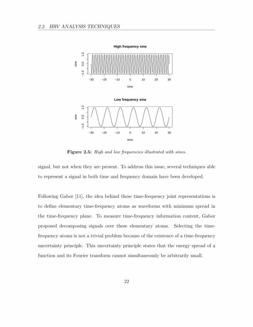
is a tool that is able to extract the frequencies of a signal. For those unfamiliar with
the “frequency” language, we will say that a signal with fast and sharp changes has
“high frequencies”, whereas a signal with slow transitions is referred to as a signal
with “low frequencies” (see Figure 2.5). Of course, a signal can contain both low and
high frequencies. In this sense, the Fourier transform acts as a prism, separating
the high frequency contributions from the low frequency contributions. The discrete
implementation is referred to as the Discrete Fourier Transform (DFT) and its
efficient implementation is called the Fast Fourier Transform (FFT).
The Fourier transform is one of the most powerful tools for signal processing.
However, it may not be the most suitable tool for studying transient phenomena:
the Fourier transform might be able to determine all the frequencies present in a
21
2.2. HRV ANALYSIS TECHNIQUES
−30 −20 −10 0 10 20 30−
1.0
0.0
1.0
High frequency sine
time
sine
−30 −20 −10 0 10 20 30
−1.
00.
01.
0
Low frequency sine
time
sine
Figure 2.5: High and low frequencies illustrated with sines.
signal, but not when they are present. To address this issue, several techniques able
to represent a signal in both time and frequency domain have been developed.
Following Gabor [11], the idea behind these time-frequency joint representations is
to define elementary time-frequency atoms as waveforms with minimum spread in
the time-frequency plane. To measure time-frequency information content, Gabor
proposed decomposing signals over these elementary atoms. Selecting the time-
frequency atoms is not a trivial problem because of the existence of a time-frequency
uncertainty principle. This uncertainty principle states that the energy spread of a
function and its Fourier transform cannot simultaneously be arbitrarily small.
22

2.2. HRV ANALYSIS TECHNIQUES
The simplest transform that uses this idea is the windowed Fourier transform, that
is constructed by using a symmetric window that selects the portion of the signal
that is going to be analyzed. The remaining portions of signal can be selected by
translating the window in time. When this transform is applied to discrete signals,
it is referred to as the Short Time Fourier Transform (STFT).
Another widely used transform that uses time-frequency atoms is the wavelet trans-
form. A wavelet is a “small wave” with zero mean that grows and decays in a limited
time period. Since any of these small waves results in different wavelets, there are
several wavelet families. Figure 2.6 shows two such wavelets. The reference wavelet
fulfilling the above conditions is called “mother wavelet”. The mother wavelet can
be translated and dilated in time, yielding a set of wavelet functions with different
sizes and centered in different time positions. This set of functions is used to ex-
tract time-frequency information by correlating them with the signal being analyzed.
Although the idea of the wavelet transform is similar to that used in the STFT, the
wavelet transform often provides a better compromise between time and frequency
resolution. This is due to the fact that the STFT uses just one window for “ex-
ploring” all the frequency bands. However, the ideal approximation would be using
short windows at high frequencies and long windows at low frequencies. Thus, the
“global” performance of the STFT will depend on the choice of the length of the
window and the displacement time used for moving it. The wavelet transform, in
contrast to the STFT, follows the ideal approximation, leading to a multiresolution
23

2.2. HRV ANALYSIS TECHNIQUES
analysis. RHRV has support for both approaches, and they both have a similar
computational efficiency.
Figure 2.6: Two wavelets. The top of the figure shows the Morlet wavelet. The bottomof the figure shows a Gaussian wavelet.
When working with frequency methods, researchers are especially interested in the
VLF, LF and HF frequency bands. Some authors also include the ULF band. When
selecting the frequency bands, the researchers should take into account whether
they are working with short (2-5 min) or long term recordings (up to 24-hours).
Three main spectral components are distinguished in a spectrum calculated from
short-term recordings: VLF, LF and HF components. However, VLF assessed from
short-term recordings is a dubious parameter and, therefore, it should be avoided
when interpreting the PSD in this type of recordings [9]. Spectral analysis resulting
from long-term recordings include VLF, LF and HF bands. In the long recordings,
the VLF band may be split into the ULF and the VLF components.
24

2.2. HRV ANALYSIS TECHNIQUES
2.2.3 Nonlinear Methods
There is a profound connection between nonlinear phenomena and HRV. HRV is
determined by complex interactions of electrophysiological and humoral variables,
as well as by autonomic and central nervous regulations. Considering these complex
control systems modulating the heart rhythm, it has been speculated that methods
of the nonlinear dynamics might extract some valuable information from the HRV
series.
A wide variety of nonlinear statistics have already been used in the HRV literature,
including largest Lyapunov exponent, generalized correlation dimension, SD1/SD2
of Poincare plots, detrended fluctuation analysis, sample entropy and recurrence
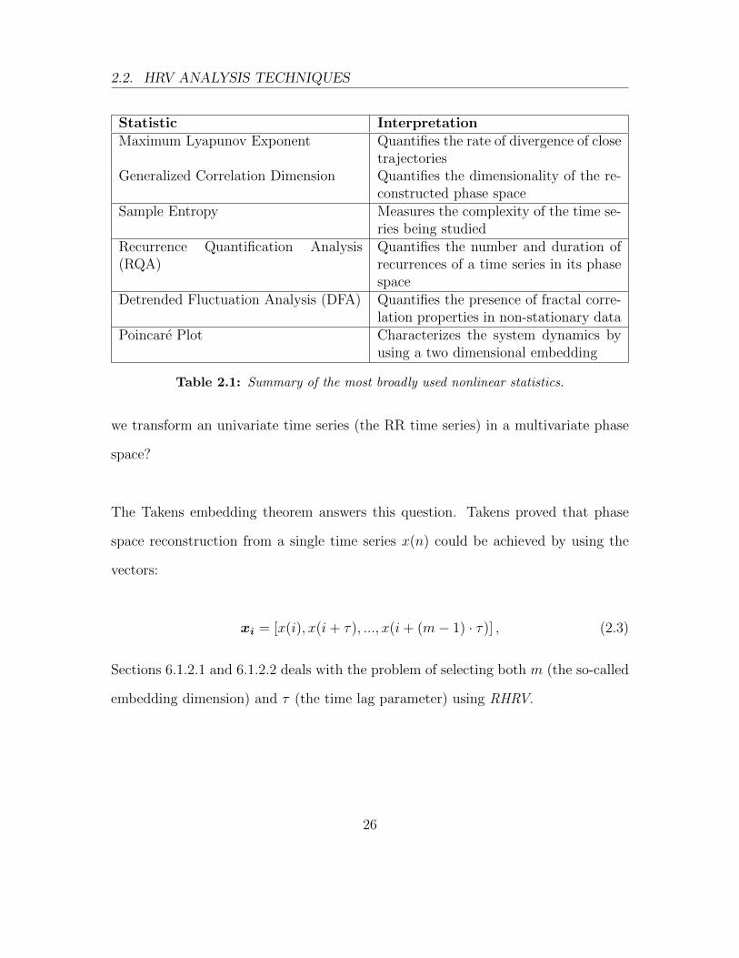
quantification analysis. Table 2.1 summarizes the most important nonlinear statis-
tics that have been included in RHRV. In the next sections, we shall present a
quick theoretical review of all these methods. More details will be given later in the
tutorial when we show how to use these methods in RHRV.
2.2.3.1 Phase space reconstruction
A large amount of nonlinear algorithms is based on the concept of phase space.
For a deterministic system, the phase space is the collection of all possible system
states. That is, each point of the phase space represents all the information needed
to determine the evolution of the system. Of course, the problem now is: How can
25
2.2. HRV ANALYSIS TECHNIQUES
Statistic InterpretationMaximum Lyapunov Exponent Quantifies the rate of divergence of close
trajectoriesGeneralized Correlation Dimension Quantifies the dimensionality of the re-
constructed phase spaceSample Entropy Measures the complexity of the time se-
ries being studiedRecurrence Quantification Analysis(RQA)
Quantifies the number and duration ofrecurrences of a time series in its phasespace
Detrended Fluctuation Analysis (DFA) Quantifies the presence of fractal corre-lation properties in non-stationary data
Poincare Plot Characterizes the system dynamics byusing a two dimensional embedding
Table 2.1: Summary of the most broadly used nonlinear statistics.
we transform an univariate time series (the RR time series) in a multivariate phase
space?
The Takens embedding theorem answers this question. Takens proved that phase
space reconstruction from a single time series x(n) could be achieved by using the
vectors:
xi = [x(i), x(i+ τ), ..., x(i+ (m− 1) · τ)] , (2.3)
Sections 6.1.2.1 and 6.1.2.2 deals with the problem of selecting both m (the so-called
embedding dimension) and τ (the time lag parameter) using RHRV.
26

2.2. HRV ANALYSIS TECHNIQUES
2.2.3.2 Correlation dimension
The correlation dimension is the most common measure of the fractal dimensionality
of a geometrical object embedded in a phase space. The estimation of the correla-
tion dimension requires the computation of the so-called correlation sum C(r). The
correlation sum is defined over the N points from the phase space as follows:
C(r) =#{(xi,xj) : distance(xi,xj) < r}
N2,
where # represents the cardinality of the set and r a radius in the embedding
dimension. However, this estimator is biased when the pairs in the sum are not
statistically independent. For example, Taken’s vectors that are close in time, are
usually close in the phase space due to the non-zero autocorrelation of the original
time series. This is solved by using the so-called Theiler window: two Takens’ vectors
must be separated by, at least, the time steps specified by this window in order
to be considered neighbours. By using a Theiler window, we exclude temporally
correlated vectors from our estimations.
Chaotic attractors are expected to fulfill
C(r) ∝ rD,
being D the correlation dimension that we want to estimate. Thus, the correlation
dimension may be estimated using the slope obtained by performing a linear regres-
sion of log10(C(r)) Vs. log10(r). Since this dimension is supposed to be an invariant
27

2.2. HRV ANALYSIS TECHNIQUES
of the system, it should not depend on the dimension of the Taken’s vectors used to
estimate it (provided that we are using an embedding dimension that is large enough
to reconstruct the phase space). Thus, the user should plot log(C(r)) Vs. log(r)
for several embedding dimensions when looking for the correlation dimension and,
if for some range log(C(r)) shows a similar linear behaviour in different embedding
dimensions (i.e. parallel slopes), these slopes are an estimate of the correlation di-
mension. This is very important! If the slope depends on the embedding dimension
(provided that we are embedding the time series in a phase space with sufficient
dimensions) we cannot talk about a correlation dimension. Furthermore, the time
series may not be chaotic. More details about this requirement shall be given when
presenting the RHRV functionality for computing the correlation dimension.
2.2.3.3 Generalized correlation dimension
Note that the correlation sum C(r) may be interpreted as: C(r) =< p(r) >, that is:
the mean probability of finding a neighbour in a ball of radius r surrounding a point
in the phase space. Thus, it is possible to define a generalization of the correlation
dimension by writing:
Cq(r) =< p(r)(q−1) > .
With this notation, the “classic” correlation sum is C(r) = C2(r). It is possible to
determine generalized dimensions Dq using the slope obtained by performing a linear
regression of log(Cq(r)) V s. (q − 1)log(r). The case q = 1 leads to the information
28

2.2. HRV ANALYSIS TECHNIQUES
dimension, that is treated separately in this package. see Sections 2.2.3.4 and 6.2.3).
The considerations discussed for the correlation dimension estimate are also valid for
these generalized dimensions.
2.2.3.4 Information dimension
The information dimension is a particular case of the generalized correlation dimen-
sion when setting the order q = 1. It is possible to demonstrate that it can be defined
as:
D1 = limr→0 < log p(r) > / log(r), (2.4)
being D1 the information dimension, p(r) is the probability of finding a neighbour
in a neighbourhood of size r and <> is the mean value. Thus, the information
dimension specifies how the average Shannon information scales with the radius r.
In order to estimate D1 in practical applications, a variation of equation 2.4 is used.
This algorithm looks for the scaling behaviour of the average radius that contains a
given portion (a ”fixed-mass”p) of the total points in the phase space. By performing
a linear regression of log(p) V s. log(< r >), an estimate of D1 is obtained.
2.2.3.5 Sample entropy
The sample entropy measures the complexity of a time series. Large values of the
Sample Entropy indicate high complexity whereas that smaller values characterize
more regular signals. The sample entropy of order q is computed in the RHRV
29

2.2. HRV ANALYSIS TECHNIQUES
package by using the correlation sums calculated with the CalculateCorrDim. We
first define the function:
hq(m, r) = log
(Cq(m, r)
Cq(m+ 1, r)
),
where m is the embedding dimension and q the order of the correlation sum. The
Sample entropy (or Renyi entropy) of order q Hq fulfills
Hq = lim r→0m→∞
hq(m, r). (2.5)
2.2.3.6 Maximum Lyapunov exponent
Close trajectories diverge exponentially fast in a chaotic system. The averaged expo-
nent that determines the divergence rate is called the Lyapunov exponent (usually de-
noted with λ). If δ(0) is the distance between two Takens’ vectors in a m-dimensional
space, we expect that the distance after a time t between the two trajectories arising
from this two vectors fulfills:
δ(t) ∝ δ(0) · exp(λt).
Thus, the Lyapunov exponent is estimated using the slope obtained by performing
a linear regression of S(t) = λ · t ≈ log(δ(t)/δ(0)) on t. In practical applications, we
should check the existence of a linear region when plotting S(t) Vs. t. If for some
temporal range this plot shows a linear behaviour, its slope is an estimate of the
maximal Lyapunov exponent per unit of time. If such a region does not exist, the
30

2.2. HRV ANALYSIS TECHNIQUES
estimation should be discarded.
Also, just as for the correlation dimension computations, the maximal Lyapunov
exponent should be computed for several embedding dimensions in order to check
that it does not depend on the embedding dimension.
2.2.3.7 Detrended Fluctuation Analysis (DFA)
The Detrended Fluctuation Analysis (DFA) is a widely used technique for detecting
correlations in time series. These functions are able to estimate several scaling expo-
nents from the RR time series being analyzed. These scaling exponents characterize
short or long-term fluctuations. The DFA procedure may be summarized as follows:
1. Integrate the time series to be analyzed. The time series resulting from the
integration will be referred to as the profile.
2. Divide the profile into N non-overlapping segments.
3. Calculate the local trend for each of the segments using least-square regression.
Compute the total error for each of the segments.
4. Compute the average of the total error over all segments and take its root
square. By repeating the previous steps for several segment sizes (let’s denote
it by t: number of beats), we obtain the so-called fluctuation function F (t).
5. If the data presents long-range power law correlations: F (t) ∝ tα, we can
estimate the exponent using regression.
31

2.2. HRV ANALYSIS TECHNIQUES
6. Usually, when plotting log(F (t)) Vs log(t) we may distinguish two linear re-
gions. By performing a regression on each of them separately, we obtain two
scaling exponents, α1 (the exponent for small values of t, characterizing short-
term fluctuations) and α2 (the exponent for large values of t, characterizing
long-term fluctuations).
2.2.3.8 Recurrence Quantification Analysis (RQA)
The Recurrence Quantification Analysis (RQA) is an advanced technique for the
nonlinear analysis that allows to quantify the number and duration of the recurrences
in the phase space. A recurrence is a time instant in which the trajectory returns to a
phase space region it has visited before. Thus, it is a representation of those instants
of time in which xi ≈ xj) for every i and j. The recurrence plot is the graphical
representation of the recurrence matrix of the RR time series. The RQA function
allows to compute several statistics derived from the RQA analysis of the RR time
series. Table 2.2 summarize the most important RQA statistics and its meaning.
2.2.3.9 Poincare plot
The Poincare plot is a graphical representation of the dependance between successive
RR intervals obtained by plotting the RRj+τ as a function of RRj. This dependance
is often quantified by fitting an ellipse to the plot. In this way, two parameters
are obtained characterizing the ellipse: SD1 and SD2. When τ = 1, SD1 is usually
calculated as the standard deviation of the points perpendicular to the line of identity
32

2.2. HRV ANALYSIS TECHNIQUES
Statistic RHRV name Interpretation
Recurrence REC Percentage of recurrencepoints in a RecurrencePlot
Determinism DET Percentage of recurrencepoints that form diagonallines
Laminarity LAM Percentage of recurrentpoints that form verticallines
Ratio RATIO Ratio between DET andRR
Longest diagonal line Lmax Length of the longest di-agonal line
Averaged diagonal linelength
Lmean Mean length of the diago-nal lines. The main diag-onal is not taken into ac-count
Divergence DIV Inverse of LmaxLongest vertical line Vmax Longest vertical lineTrapping time Vmean Average length of the ver-
tical lines.Entropy ENTR Shannon entropy of the
diagonal line lengths dis-tribution
Trend TREND Trend of the number ofrecurrent points depend-ing on the distance to themain diagonal
Recurrence Rate recurrenceRate Number of recurrentpoints depending on thedistance to the maindiagonal
Table 2.2: Most important RQA statistics.
33

2.3. HRV ALTERATIONS RELATED TO SPECIFIC PATHOLOGIES
and SD2 is calculated as the standard deviation along the line of identity. In terms
of time-domain parameters:
SD21 =
1
2SDSD2
SD22 = 2 · SDNN2 − 1
2SDSD2
In this way SD1 characterizes short-term variability whereas that SD2 character-
izes long-term variability. However, sometimes the ellipse that is fitted using this
approach is too small. RHRV also allows the user to fit a ellipse by estimating a
confidence region. If τ > 1, the confidence region approach is always used. More
details shall be given in 6.2.4.
2.3 HRV alterations related to specific patholo-
gies
In the course of the last two decades numerous studies have shown HRV to be
a useful tool as a predictor of several pathologies such as myocardial infarction,
sudden cardiac death, heart failure, hypertension, and ischemia, among others [22].
However, it should be noted that the practical use of HRV has reached general
consensus only in two clinical applications: as a predictor of risk after myocardial
infarction and as an early warning of diabetic neuropathy. [9], [18].
Table 2.3 resumes some HRV applications to other diseases.
34

2.3. HRV ALTERATIONS RELATED TO SPECIFIC PATHOLOGIES
Table 2.3: Summary of the clinical value of HRV analysis in cardiological diseases. In-spired by [9].
Disease state Clinical finding Potential value
Myocardial infarction (MI) ↓ HRV after myocardial infarc-
tion (MI). In the severe phase
of MI, there is a ↓ standard de-
viation of the HRV signal
Depressed HRV is a power-
ful predictor of mortality and
of arrhythmic complications in
patients following acute MI
HRV analysis is useful for risk
stratification of patients fol-
lowing MI
Diabetic neuropathy ↓ time-domain parameters of
HRV preceded the clinical de-
tection of autonomic neuropa-
thy. ↓ LF and HF bands in di-
abetic patients with no signs of
autonomic neuropathy
HRV analysis may be used
as predictor of diabetic auto-
nomic neuropathy occurrence
Hypertension ↑ LF found in hypertensives
with circadian patterns
Hypertension is characterized
by depressed circadian rhyth-
micity of LF
Reduced parasympathetic ac-
tivity in hypertensive patients
Congestive heart failure (CHF) ↓ spectral power in all frequen-
cies, especially > 0.04 Hz
In CHF, there is ↓ vagal,
but relatively preserved sym-
pathetic modulation of HR
Low HRV Reduced vagal activity in CHF
patients
↓ HF power in CHF.↑ LF/HF Low parasympathetic tone in
CHF. CHF produces imbal-
ance of autonomic tone with ↓
parasympathetic and predomi-
nance of sympathetic tone
Continued on next page
35

2.3. HRV ALTERATIONS RELATED TO SPECIFIC PATHOLOGIES
Table 2.3 – continued from previous page
Disease state Clinical findings Potential value
Alterations in HRV not tightly
linked to severity of CHF. ↓
HRV was related to sympa-
thetic excitation
↑ HRV during ACE
(angiotensin-converting-
enzyme) inhibitor treatment
Increase of the sympathetic
tone associated with ACE in-
hibitor therapy
Heart Transplantation HRV from 0.02 to 1 Hz is 90%
reduced
Patients with rejection show
less variability
Chronic mitral regurgitation HR techniques correlated with
ventricular performance and
predicted clinical events
Prognostic indicator of atrial
fibrillation, mortality and pro-
gression to valve surgery
Mitral Valve prolapse (MVP) ↓ HF power MVP patients had low vagal
tone
Cardiomyopathies Global and specific vagal tone
measurements of HRV were ↓
in symptomatic patients
Sudden death (SD) or cardiac
arrest (CA)
LF power and standard devi-
ation of HRV signals were re-
lated to 1 year mortality
HRV is useful to risk stratify
CA survivors for 1 year mor-
tality
↓ HF power in CA survivors
Both time and frequency do-
main indexes separated con-
trols from SD patients. ↓ HF
power was the best separator
between heart disease patients
with and without SD
HF power may be useful pre-
dictor of SD
SDNN index was lower in SD
patients
Time domain indexes may
identify increased risk of SD
Continued on next page
36

2.3. HRV ALTERATIONS RELATED TO SPECIFIC PATHOLOGIES
Table 2.3 – continued from previous page
Disease state Clinical findings Potential value
Ventricular arrhythmias HRV indexes do not change
consistently before ventricular
fibrillation (VF). All power
spectra of HRV were signifi-
cantly ↓ before the onset of
sustained ventricular tachycar-
dia (VT) than before non sus-
tained VT
A temporal relation exists be-
tween the decrease of HRV and
the onset of sustained VT
37

Chapter 3
Installation
3.1 Installation
This guide assumes that the user has some basic knowledge of the R environment. If
this is not your case, you can find a nice introduction to R in the R project homepage
[3]. The R project homepage also provides an “R Installation and Administration”
guide. Once you have download and installed R, you can install RHRV by typing:
> install.packages("RHRV")
You can also install it by downloading it from the CRAN [2]. Once the download
has finished, open R, move to the directory where you have download it (by using
the R command setwd) and type:
> install.packages("RHRV_XXX",repos=NULL)
Here, XXX is the version number of the library. To start using the library, you should
load it by using the library command:
38

3.2. WFDB APPLICATIONS
> library(RHRV)
3.2 WFDB applications
Some functions of the RHRV package (such as the LoadApneaWFDB) require the
installation of the WFDB functions [25]. If the user is not going to work with WFDB
formatted files, the installation of these libraries is not required for the proper func-
tioning of RHRV. The WFDB functions is a large collection of specialized software for
processing and manipulating the PhysioNet’s databases [14]. On Windows and Mac
OSX operating systems is necessary to define a .Renviron file in the user workspace
indicating the directory of the WFDB commands. Examples for both OS are given
below:
## .Renviron on Windows
PATH = "c:\\cygwin\\bin"
DYLD_LIBRARY_PATH = "c:\\cygwin\\lib"
## .Renviron on Macosx
PATH = "/opt/local/bin"
DYLD_LIBRARY_PATH = "/opt/local/bin"
39
3.3. TROUBLESHOOTING
3.3 Troubleshooting
3.3.1 When installing the RHRV package in linux, some-
times the installation fails when installing the tkrplot
dependency.
...
tcltkimg.c:2:16: fatal error: tk.h: No such file or directory
compilation terminated.
ERROR: compilation failed for package 'tkrplot'
...
ERROR: dependency 'tkrplot' is not available for package 'RHRV'
This is usually because there are some missing libraries in your system. Generally,
the problem will be fixed by installing the tclX.X, tkX.X, tclX.X-dev and tkX.X-dev
libraries (X.X stands for the version of the libraries).
40

Chapter 4
A 15-minutes guide to RHRV
In this chapter, a brief description of the RHRV package is presented [30]. Due
to the large collection of features that RHRV offers, in this chapter we shall refer
only to the most important functionality for performing a basic HRV analysis. In
the next chapter we will present more advanced functionality of the package, or
functionality geared to certain particular types of analysis. RHRV can be freely
downloaded from the R-CRAN repository [2].
We propose the following basic program flow to perform HRV analysis using the
RHRV package:
1. Load heart beat positions. For the sake of simplicity, in this section we will
focus in ASCII files.
2. Build the instantaneous HR series and filter it to eliminate spurious points.
3. Plot the instantaneous HR series.
41

4. Interpolate the instantaneous HR series to obtain a HR series with equally
spaced values.
5. Plot the interpolated HR series.
6. Perform the desired analysis. The user can perform time-domain analysis,
frequency-domain analysis and/or nonlinear analysis.
7. Plot the results of the analysis that has been performed and access the “raw”
data.
In section 4.1 we will address points 1-5, whereas in section 4.2 we will deal with
points 6 and 7. All the examples of this chapter will use the example beats file “ex-
ample.beats” that may be downloaded from http://rhrv.r-forge.r-project.org/. Adi-
tionally, the data from this file has been included in RHRV. The user can access this
data executing:
> # HRVData structure containing the heart beats
> data("HRVData")
> # HRVData structure storing the results of processing the
> # heart beats: the beats have been filtered, interpolated, ...
> data("HRVProcessedData")
The example file is an ASCII file that contains the beat positions obtained from
a 2 hours ECG (one beat position per row). The subject of the ECG is a patient
suffering from paraplegia and hypertension (systolic blood pressure above 200
mmHg). During the recording, he is supplied with prostaglandin E1 (a vasodilator
42
4.1. PREPROCESSING THE HEART RATE SERIES
that is rarely employed) and systolic blood pressure fell to 100 mmHg for over an
hour. Then, the blood pressure increased slowly up to approximately 150 mmHg.
The console output shall be shown for every example.
4.1 Preprocessing the Heart Rate series
4.1.1 Load heart beat positions
RHRV uses a custom data structure called HRVData to store all HRV information
related to the signal being analyzed. HRVData is implemented as a list object in R
language. This list contains all the information corresponding to the imported signal
to be analyzed, some parameters generated by the pre-processing functions and the
HRV analysis results. A new HRVData structure is created using the CreateHRVData
function. In order to obtain detailed information about the operations performed by
the program, we can activate a verbose mode using the SetVerbose function.
> hrv.data = CreateHRVData()
> hrv.data = SetVerbose(hrv.data, TRUE )
After creating the empty HRVData structure the next step should be loading the sig-
nal that we want to analyze into this structure. RHRV imports data files containing
heart beat positions. Supported formats include ASCII (LoadBeatAscii function),
EDF (LoadBeatEDFPlus), Polar (LoadBeatPolar), Suunto (LoadBeatSuunto) and
WFDB data files (LoadBeatWFDB) [26]. For the sake of simplicity, we will focus
43

4.1. PREPROCESSING THE HEART RATE SERIES
in ASCII files containing one heart beat occurrence time per line. We also assume
that the beat occurrence time is specified in seconds (further details will be given in
chapter 5). For example, let’s try to load the “example.beats” file, whose first lines
are shown below. Each line denotes the occurrence time of each heartbeat.
0
0.3280001
0.7159996
1.124
1.5
1.88
In order to load this file, we may write:
> hrv.data = LoadBeatAscii(hrv.data, "example.beats",
+ RecordPath = "beatsFolder")
** Loading beats positions for record: example.beats **
Path: beatsFolder
Scale: 1
Date: 01/01/1900
Time: 00:00:00
Number of beats: 17360
The console information is only displayed if the verbose mode is on. The Scale
parameter is related to the time units of the file. 1 denotes seconds, 0.1 tenth
44
4.1. PREPROCESSING THE HEART RATE SERIES
of seconds and so on. The Date and Time parameters specify when the file was
recorded. More details about these parameters will be given in section 5.1.2. The
RecordPath can be omitted if the RecordName is in the working directory.
4.1.2 Calculating HR and filtering
To compute the HRV time series the BuildNIHR function can be used (Build Non
Interpolated Heart Rate). This function constructs both the RR (Equation 2.1) and
instantaneous heart rate (HR) series (Equation 2.2) described in Section 2.1. We
will refer to the instantaneous heart rate (HR) as the Non Interpolated Heart Rate
(niHR) series. Both series are stored in the HRVData structure.
> hrv.data = BuildNIHR(hrv.data)
** Calculating non-interpolated heart rate **
Number of beats: 17360
A filtering operation must be carried out in order to eliminate outliers or spurious
points present in the niHR time series with unacceptable physiological values.
Outliers present in the series originate both from detecting an artifact as a heartbeat
(RR interval too short) or not detecting a heartbeat (RR interval too large). The
outliers removal may be both manual or automatic. In this quick introduction, we
will use the automatic removal. The automatic removal of spurious points can be
performed by the FilterNIHR function. The FilterNIHR function also eliminates
45

4.1. PREPROCESSING THE HEART RATE SERIES
points with unacceptable physiological values.
> hrv.data = FilterNIHR(hrv.data)
** Filtering non-interpolated Heart Rate **
Number of original beats: 17360
Number of accepted beats: 17259
4.1.3 Interpolating
In order to be able to perform spectral analysis in the frequency domain, a uniformly
sampled HR series is required. It may be constructed from the niHR series by using
the InterpolateNIHR function, which uses linear (default) or spline interpolation
(further details on chapter 5). The frequency of interpolation may be specified.
4 Hz (the default value) is enough for most applications.
> # Note that it is not necessary to specify freqhr since it matches with
> # the default value: 4 Hz
> hrv.data = InterpolateNIHR (hrv.data, freqhr = 4)
** Interpolating instantaneous heart rate **
Frequency: 4Hz
Number of beats: 17259
Number of points: 29594
46

4.2. ANALYZING THE HEART RATE SERIES
4.1.4 Plotting
Before applying the different analysis techniques that RHRV provides, it is usually
interesting to plot the time series with which we are working. The PlotNIHR
function permits the graphical representation of the niHR series whereas the PlotHR
function permits to graphically represent the interpolated HR time series.
> PlotNIHR(hrv.data)
> PlotHR(hrv.data)
The plots obtained with PlotNIHR and PlotHR are shown in Figures 4.1 and 4.2,
respectively.
As seen in the Figures 4.1 and 4.2, the patient initially had a heart rate of approxi-
mately 160 beats per minute. Approximately half an hour into record the prostaglan-
dina E1 was provided, resulting in a drop in heart rate to about 130 beats per minute
during about 40 minutes, followed by a slight increase in heart rate.
4.2 Analyzing the Heart Rate series
4.2.1 Accessing “raw data”
In the previous sections, we have used the HRVData structure to store all HRV
information related to the signal being analyzed with no knowledge about its internal
47

4.2. ANALYZING THE HEART RATE SERIES
0 2000 4000 6000
8010
012
014
016
018
020
0
time (sec.)
HR
(be
ats/
min
.)
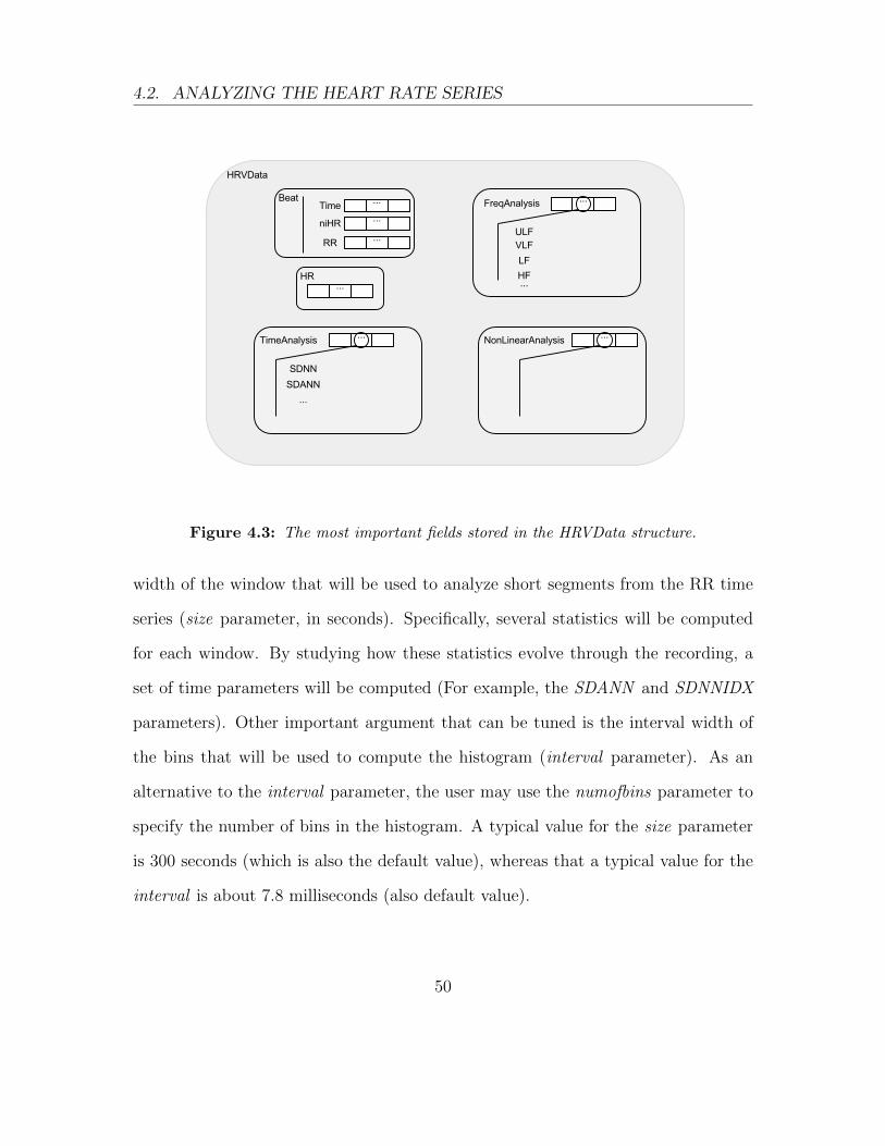
Non−interpolated instantaneous heart rate
Figure 4.1: Non interpolated Heart Rate time plot example.
structure. However, sometimes, in order to make some particular analysis of the
data, it may be interesting to access them directly. Figure 4.3 summarizes the most
important fields in the HRVData structure. Since all the data in this structure is
stored as an R list, each of its fields can be accessed using the $ operator of the R
language. For example, if we want to access the RR time series of the hrv.data, we
would use:
> RR = hrv.data$Beat$RR
Although it is an advantage to be familiarized with the HRVData structure, there
is no need to memorize it since we can use the useful name R function. Thus, if we
want to know which fields are stored into the hrv.data$Beat subfield, we could use:
48

4.2. ANALYZING THE HEART RATE SERIES
0 2000 4000 6000
8010
012
014
016
018
0
time (sec.)
HR
(be
ats/
min
.)
Interpolated instantaneous heart rate
Figure 4.2: Interpolated Heart Rate time plot example.
> names(hrv.data$Beat)
[1] "Time" "niHR" "RR"
As we can see, hrv.data$Beat stores the occurrence time of each beat (“Time”), the
niHR time series (“niHR”) and the RR time series (“RR”).
4.2.2 Time-domain analysis techniques
The simplest way of performing a HRV analysis in RHRV is using the time analysis
techniques provided by the CreateTimeAnalysis function. This function computes
the time-domain parameters presented in Section 2.2.1 and stores them in the HRV-
Data structure. The most interesting parameter that the user may specify is the
49
4.2. ANALYZING THE HEART RATE SERIES
Figure 4.3: The most important fields stored in the HRVData structure.
width of the window that will be used to analyze short segments from the RR time
series (size parameter, in seconds). Specifically, several statistics will be computed
for each window. By studying how these statistics evolve through the recording, a
set of time parameters will be computed (For example, the SDANN and SDNNIDX
parameters). Other important argument that can be tuned is the interval width of
the bins that will be used to compute the histogram (interval parameter). As an
alternative to the interval parameter, the user may use the numofbins parameter to
specify the number of bins in the histogram. A typical value for the size parameter
is 300 seconds (which is also the default value), whereas that a typical value for the
interval is about 7.8 milliseconds (also default value).
50

4.2. ANALYZING THE HEART RATE SERIES
> hrv.data = CreateTimeAnalysis(hrv.data, size = 300,
+ interval = 7.8125)
** Creating time analysis
Size of window: 300 seconds
Width of bins in histogram: 7.8125 milliseconds
Number of windows: 24
Data has now 1 time analyses
SDNN: 39.81504 msec.
SDANN: 31.11223 msec.
SDNNIDX: 25.05384 msec.
pNN50: 9.39854 %
SDSD: 31.07026 msec.
r-MSSD: 31.06936 msec.
IRRR: 32 msec.
MADRR: 16 msec.
TINN: 86.10213 msec.
HRV index: 11.02107
If the verbose mode is on, the program will display the results of the calculations on
the screen. Otherwise, the user must access the “raw” data as explained before to
obtain the results.
Finally, we show a complete example for performing a basic time-domain analysis.
The console output is also shown. It should be noted that it is not necessary to
51

4.2. ANALYZING THE HEART RATE SERIES
perform the interpolation process before applying the time-domain techniques since
these parameters are calculated directly from the RR-time series.
> hrv.data = CreateHRVData()
> hrv.data = SetVerbose(hrv.data,FALSE)
> hrv.data = LoadBeatAscii(hrv.data,"example.beats","beatsFolder")
> hrv.data = BuildNIHR(hrv.data)
> hrv.data = FilterNIHR(hrv.data)
> PlotNIHR(hrv.data)
> hrv.data = SetVerbose(hrv.data,TRUE)
> hrv.data = CreateTimeAnalysis(hrv.data,size=300,interval = 7.8125)
** Creating time analysis
Size of window: 300 seconds
Width of bins in histogram: 7.8125 milliseconds
Number of windows: 24
Data has now 1 time analyses
SDNN: 39.81504 msec.
SDANN: 31.11223 msec.
SDNNIDX: 25.05384 msec.
pNN50: 9.39854 %
SDSD: 31.07026 msec.
r-MSSD: 31.06936 msec.
IRRR: 32 msec.
52

4.2. ANALYZING THE HEART RATE SERIES
MADRR: 16 msec.
TINN: 86.10213 msec.
HRV index: 11.02107
> # We can access "raw" data... let's print separately, the SDNN
> # parameter
> cat("The SDNN has a value of ",hrv.data$TimeAnalysis[[1]]$SDNN," msec.\n")
The SDNN has a value of 39.81504 msec.
4.2.3 Frequency-domain analysis techniques
A major part of the functionality of the RHRV package is dedicated to the spectral
analysis of HR signals. Before performing the frequency analysis, a data analysis
structure must be created. Such structure shall store the information extracted
from a variability analysis of the HR signal as a member of the FreqAnalysis list,
under the HRVData structure. Each analysis structure created is identified by a
unique number (in order of creation). To create such an analysis structure, the
CreateFreqAnalysis function is used.
> hrv.data = CreateFreqAnalysis(hrv.data)
** Creating frequency analysis
Data has now 1 frequency analysis
Notice that, if verbose mode is on, the CreateFreqAnalysis function informs us about
the number of frequency analysis structures that have been created. In order to
53

4.2. ANALYZING THE HEART RATE SERIES
select a particular spectral analysis, we will use the indexFreqAnalysis parameter in
the frequency analysis functions.
The most important function to perform spectral HRV analysis is the Calcu-
latePowerBand function. The CalculatePowerBand function computes the spectro-
gram of the HR series in the ULF, VLF, LF and HF frequency bands using STFT
or wavelets. Boundaries of the bands may be chosen by the user. If boundaries are
not specified, default values are used: ULF, [0, 0.03] Hz; VLF, [0.03, 0.05] Hz; LF,
[0.05, 0.15] Hz; HF, [0.15, 0.4] Hz. The type of analysis can be selected by the user
by specifying the type parameter of the CalculatePowerBand function. The possible
options are either “fourier” or “wavelet”. Because of the backwards compatibility,
the default value for this parameter is “fourier”.
4.2.3.1 Fourier
When using the STFT to compute the spectrogram employing the CalculatePower-
Band function, the user may specify the following parameters related with the STFT:
• Size: the size of window for calculating the spectrogram measured in seconds.
The RHRV package employs a Hamming window to perform the STFT.
• Shift : the displacement of window for calculating the spectrogram measured
in seconds.
54
4.2. ANALYZING THE HEART RATE SERIES
• Sizesp: the number of points for calculating each window of the STFT. Thus,
it is highly recommended to select sizesp so that sizesp = 2N . If the user does
not specify it, the program selects a proper length for the calculations.
When using CalculatePowerBand, the indexFreqAnalysis parameter (in order to
indicate which spectral analysis we are working with) and the boundaries of the
frequency bands may also be specified.
As an example, let’s perform a frequency analysis in the typical HRV spectral bands
based on the STFT . We may select 300 s (5 minutes) and 30 s as window size and
displacement values because these are typical values when performing HRV spectral
analysis. The value of the zero-padding should be chosen to be greater than the
number of samples of the window size. Assuming that the sampling frequency is
4 Hz, the zero-padding value must fulfill sizesp ≥ size · fs. In this occasion, we
select the smallest power of 2 that meets the previous condition: sizesp = 2048 =
211 > 1200 = 300 · 4. Thus, we may write:
> hrv.data = CreateHRVData( )
> hrv.data = SetVerbose(hrv.data,FALSE)
> hrv.data = LoadBeatAscii(hrv.data,"example.beats","beatsFolder")
> hrv.data = BuildNIHR(hrv.data)
> hrv.data = FilterNIHR(hrv.data)
> hrv.data = InterpolateNIHR (hrv.data, freqhr = 4)
> hrv.data = CreateFreqAnalysis(hrv.data)
> hrv.data = SetVerbose(hrv.data,TRUE)
55

4.2. ANALYZING THE HEART RATE SERIES
> # Note that it is not necessary to write the boundaries
> # for the frequency bands, since they match
> # the default values
> hrv.data = CalculatePowerBand( hrv.data , indexFreqAnalysis= 1,
+ size = 300, shift = 30, sizesp = 2048, type = "fourier",
+ ULFmin = 0, ULFmax = 0.03, VLFmin = 0.03, VLFmax = 0.05,
+ LFmin = 0.05, LFmax = 0.15, HFmin = 0.15, HFmax = 0.4 )
** Calculating power per band **
** Using Fourier analysis **
Windowing signal... 237 windows
Power per band calculated
Alternatively, we could not specify the sizesp parameter and let the program decide
for us. In fact, the program would use the same criteria that we used in the previous
example. Thus, we could have used the following sentence to obtain exactly the same
results:
> hrv.data = CalculatePowerBand( hrv.data , indexFreqAnalysis= 1,
+ size = 300, shift = 30 )
4.2.3.2 Wavelets
When using wavelet analysis with the CalculatePowerBand function, the user may
specify:
56

4.2. ANALYZING THE HEART RATE SERIES
• Wavelet : mother wavelet used to calculate the spectrogram. Some of the most
widely used wavelets are available: Haar (“haar”), extremal phase (“d4”, “d6”,
“d8” and “d16”) and the least asymmetric Daubechies (“la8”, “la16” and “la20”)
and the best localized Daubechies (“bl14” and “bl20”) wavelets among oth-
ers. The default value is “d4”. The name of the wavelet specifies the “family”
(the family determines the shape of the wavelet and its properties) and the
length of the wavelet. For example, “la8” belongs to the Least Asymmetric
family and has a length of 8 samples. We may give a simple advice for wavelet
selection based on the wavelet’s length: shorter wavelets usually have better
temporal resolution, but worse frequency resolution. On the other hand, longer
wavelets usually have worse temporal resolution, but they provide better fre-
quency resolution. Better temporal resolution means that we can study shorter
time intervals. On the other hand, a better frequency resolution means better
“frequency discrimination”. That is, shorter wavelets will tend to fail when
discriminating close frequencies.
• Bandtolerance: maximum error allowed when the wavelet-based analysis is
performed [12], [13]. It can be specified as either an absolute or a relative error
depending on the “relative” parameter value. Default value is 0.01.
• Relative: logic value specifying which type of band tolerance shall be used:
relative (in percentage) or absolute (default value).
Let [fl, fu] be any frequency band specified by the user and let [f1, f2] be a frequency
interval associated with some node in the
57

4.2. ANALYZING THE HEART RATE SERIES
Maximal Overlap Discrete Wavelet Packet Transform (MODWPT) tree [29].
The relative error εr of fl over the [f1, f2] interval is computed as
εr =∣∣∣fl − f1
fu − fl
∣∣∣ · 100%.
Similarly, we may define the error εr of the upper frequency fu as
εr =∣∣∣fu − f2
fu − fl
∣∣∣ · 100%.
The relative error can be used to avoid introducing large errors at small frequency
bands (usually both ULF and VLF bands).
The absolute value ε is defined as usual: ε = |f2 − fu| for the upper frequency and
ε = |f1 − fl| for the lower frequency.
Let’s analyze the same frequency bands as before but using the wavelet-algorithm.
For the sake of simplicity, we will use an absolute tolerance of 0.01 Hz. We may
select the least asymmetric Daubechies of width 8 (“la8”) as wavelet, since it provides
a good compromise between frequency and time resolution. Thus, we may write:
> hrv.data = CreateHRVData( )
> hrv.data = SetVerbose(hrv.data,FALSE)
> hrv.data = LoadBeatAscii(hrv.data,"example.beats","beatsFolder")
> hrv.data = BuildNIHR(hrv.data)
> hrv.data = FilterNIHR(hrv.data)
58

4.2. ANALYZING THE HEART RATE SERIES
> hrv.data = InterpolateNIHR (hrv.data, freqhr = 4)
> hrv.data = CreateFreqAnalysis(hrv.data)
> hrv.data = SetVerbose(hrv.data,TRUE)
> # Note that it is not necessary to write the boundaries
> # for the frequency bands, since they match the default values
> hrv.data = CalculatePowerBand( hrv.data , indexFreqAnalysis= 1,
+ type = "wavelet", wavelet = "la8", bandtolerance = 0.01, relative = FALSE,
+ ULFmin = 0, ULFmax = 0.03, VLFmin = 0.03, VLFmax = 0.05,
+ LFmin = 0.05, LFmax = 0.15, HFmin = 0.15, HFmax = 0.4 )
** Calculating power per band **
** Using Wavelet analysis **
Power per band calculated
4.2.3.3 Creating several analyses
In the previous examples we have used just one frequency analysis to illustrate the
basic use of CalculatePowerBand. However, it is possible to create and use the same
HRVData for performing several spectral analysis. When we do this, we use the
parameter “indexFreqAnalysis” to indicate which spectral analysis we are working
with. For example, we could perform both Fourier and wavelet based analysis:
> # ...
> # create structure, load beats, filter and interpolate
> hrv.data = CreateFreqAnalysis(hrv.data)
> hrv.data = SetVerbose(hrv.data,TRUE)
59

4.2. ANALYZING THE HEART RATE SERIES
> # use freqAnalysis number 1 for perfoming
> # Fourier analysis. This time, we do not
> # write the band's boundaries
> hrv.data = CalculatePowerBand( hrv.data , indexFreqAnalysis= 1,
+ size = 300, shift = 30, sizesp = 2048, type = "fourier")
** Calculating power per band **
** Using Fourier analysis **
Windowing signal... 237 windows
Power per band calculated
> # use freqAnalysis number 2 for perfoming
> # wavelet analysis. Note the indexFreqAnalysis = 2!!!
> hrv.data = CreateFreqAnalysis(hrv.data)
** Creating frequency analysis
Data has now 2 frequency analysis
> hrv.data = CalculatePowerBand( hrv.data , indexFreqAnalysis= 2,
+ type = "wavelet", wavelet = "la8", bandtolerance = 0.01, relative = FALSE)
** Calculating power per band **
** Using Wavelet analysis **
Power per band calculated
60

4.2. ANALYZING THE HEART RATE SERIES
4.2.3.4 Plotting
RHRV also includes plotting utilities for representing the spectrogram of each fre-
quency band: the PlotPowerBand function. The PlotPowerBand receives as inputs
the HRVData structure and the index of the frequency analysis that the user wants
to plot (indexFreqAnalysis argument). Optionally, the user can specify additional
parameters for modifying the plots (whether to use or not normalized plots, specify
the y-axis, etc.). For the sake of simplicity we will only use the ymax parameter
(for specifying the maximum y-axis of the power bands plot) and the ymaxratio
parameter (for specifying the maximum y-axis in the LF/HF plot).
If we want to plot the power bands computed in the previous example, we may use:
> # Plotting Fourier analysis
> PlotPowerBand(hrv.data, indexFreqAnalysis = 1, ymax = 200, ymaxratio = 1.7)
> # Plotting wavelet analysis
> PlotPowerBand(hrv.data, indexFreqAnalysis = 2, ymax = 700, ymaxratio = 50)
The plots obtained with PlotPowerBand are shown in Figures 4.4 and 4.5, respec-
tively.
61

4.2. ANALYZING THE HEART RATE SERIES
0 50 100 150 200
0.0
1.0
LF/H
F
0 50 100 150 200
010
020
0U
LF
0 50 100 150 200
010
020
0V
LF
0 50 100 150 200
010
020
0LF
0 50 100 150 200
010
020
0
No. of frames
HF
Power bands of HRV
Figure 4.4: Plot obtained with the PlotPowerBand for the Fourier-based analysis.
4.2.3.5 A brief comparison: wavelets Vs. Fourier
Figures 4.4 and 4.5 illustrate some of the most important differences between Fourier
and wavelet-based analysis. The most important differences may be summarized as
follows:
• The power range is not the same when using Fourier than when using wavelets
due to the windowing used in both techniques. Thus, we should avoid direct
comparisons between the numerical results obtained with Fourier with those
obtained using wavelets.
62

4.2. ANALYZING THE HEART RATE SERIES
0 5000 10000 15000 20000 25000 30000
020
40LF
/HF
0 5000 10000 15000 20000 25000 30000
030
060
0U
LF
0 5000 10000 15000 20000 25000 30000
030
060
0V
LF
0 5000 10000 15000 20000 25000 30000
030
060
0LF
0 5000 10000 15000 20000 25000 30000
030
060
0
No. of frames
HF
Power bands of HRV
Figure 4.5: Plot obtained with the PlotPowerBand for the wavelet-based analysis.
• The Fourier’s power spectrum is smoother than the wavelet’s power spectrum.
This is a consequence of the higher temporal resolution that the wavelet-based
analysis provides. We could try to increase Fourier’s frequency resolution by
decreasing the window’ size used in the analysis. The shorter window we use,
the sharper spectrum we get. Similarly, we can increase/decrease temporal res-
olution using shorter/larger wavelets when performing wavelet-based analysis.
• The power spectrum obtained from the Fourier-based analysis has a smaller
number of samples than the original signal as a consequence of the use of
63

4.2. ANALYZING THE HEART RATE SERIES
windows. Conversely, the power spectrum obtained from the wavelet-based
analysis has the same number of samples as the original RR time series.
64
Chapter 5
Some more advanced features of
RHRV
5.1 Completing our first tour
In chapter 4 we have presented a brief description of the RHRV package. In this
section, we introduce some more advanced functionality of RHRV, or functional-
ity that has narrower applications than the one presented in the previous chapter.
Thus, we will introduce some new functions (EditNIHR, CalculateSpectrogram and
PlotSpectrogram) and we will finish the description of all the function parameters
introduced in the previous chapter. Also, further information about the HRVData
structure will be given. Figure 5.1 shows a detailed view of the internal organization
of the HRVData structure. This figure should be used as a roadmap through the
explanations concerning the HRVData structure.
65

5.1. COMPLETING OUR FIRST TOUR
Figure 5.1: All the fields stored in the HRVData structure.
5.1.1 Creating the structure
When a new HRVData is created using the CreateHRVData function, it contains the
following fields (among others that are not useful for the final user):
• Ext : A string that will be used as file extension by the loading/writing functions
included in the package. The default value is “hrv”.
• TimeAnalysis : This field stores the information generated using time-domain
analysis techniques. It is implemented as a list in the R language.
66

5.1. COMPLETING OUR FIRST TOUR
• FreqAnalysis : This field stores the results of one or more frequency analysis.
Frequency analysis can be based on Fourier or on wavelets. It is implemented
as a list in the R language.
• NonLinearAnalysis : This field stores the results of one or more nonlinear anal-
ysis. It is implemented as a list in the R language.
• Verbose: Boolean flag that specifies if all the functions should return additional
information (mode verbose on). The SetVerbose function sets verbose mode on
or off.
5.1.2 Reading heart beats
After creating the empty HRVData structure we will usually read the corresponding
data file containing the heart beat positions. For the sake of simplicity, we keep on
focussing on the ASCII files. The reader may have been wondering: “what happens
if my ASCII file is specified in milliseconds?”. We shall use the scale parameter to
overcome this issue. By setting this parameter to 1 (default value) we are indicating
that the beat positions are specified in seconds; by setting it to 0.1, we are indicating
that the beats are in deciseconds and so on. The function transforms the heart
beat positions to seconds so all the other functions can be used as before. Other
interesting parameter that can be specified by the user is the date-time when the
file was recorded (datetime parameter). This is particularly useful for following a
patient’s evolution over a set of recordings. The string format for the datetime
parameter is “DD/MM/YYYY HH:MM:SS”. Thus, let’s read the “example.beats”
67

5.1. COMPLETING OUR FIRST TOUR
file (as in chapter 4) specifying that it was recorded on “30/04/2012 12:00:00” in
seconds:
> hrv.data = LoadBeatAscii(hrv.data, "example.beats",
+ RecordPath = "beatsFolder", scale = 1,
+ datetime = "30/04/2012 12:00:00")
** Loading beats positions for record: example.beats **
Path: beatsFolder
Scale: 1
Date: 30/04/2012
Time: 12:00:00
Number of beats: 17360
When importing the data into the HRVData structure, two new fields are created
(see Figure 5.1):
• Datetime: Date and time associated with the record.
• Beat : A dataframe object which stores the positions of the beats in the sub-field
Time .
5.1.3 Constructing the time series
To compute the HRV time series the BuildNIHR function is used. Since we have
already used all the parameters of this function, we will focus on the HRVData
structure. As we know, this function constructs both the RR (Equation 2.1) and
68

5.1. COMPLETING OUR FIRST TOUR
instantaneous heart rate series (Equation 2.2). Both series are stored in the Beat
dataframe of the HRVData structure: the RR series is stored in the sub-field called
RR whereas the instantaneous HR is stored in the niHR sub-field (see Figure 5.1).
5.1.4 Filtering the time series
The automatic removal of outliers is performed with the FilterNIHR function. This
function implements an algorithm that uses adaptive thresholds for rejecting or ac-
cepting beats [33]. The rule for beat acceptation or rejection is to compare the present
beat with the previous one, the following one and with an updated mean of the RR
interval. The different adaptive thresholds establish an upper limit for the relative
errors of each of these comparisons. The long parameter allows the user to specify
the number of beats that shall be used to calculate the updated mean (default value
is 50 heartbeats). Also, the last parameter permits the user to specify the initial
threshold value in % (default value is 13%). Finally, the algorithm also applies a
comparison with acceptable physiological values. The user can specify the range of
acceptable physiological values by using the minbpm and maxbpm (minimum beats
per minute and maximum beats per minute, respectively). Default values are de-
signed for human beings(minbpm=25, maxbpm=200), but they can be specified in
such a way that it may also be used by animal researchers. As an illustrative exam-
ple we could modify the last parameter in such a way that it does not allow quick
fluctuations ( by decreasing last to 1%) in our example file. Also, we could decrease
69

5.1. COMPLETING OUR FIRST TOUR
the maxbpm parameter to 180 bpm. The results are shown in Figure 5.2 (compare
it with Figure 4.1).
> hrv.data = FilterNIHR(hrv.data, long=50, last=1, minbpm=25, maxbpm=180)
> PlotNIHR(hrv.data)
0 2000 4000 6000
8010
012
014
016
018
0
time (sec.)
HR
(be
ats/
min
.)
Non−interpolated instantaneous heart rate
Figure 5.2: Effects of the modification of the default values in the FilterNIHR function.
RHRV also provides functionality for manually removing the spurious heartbeats.
In order to delete outliers manually, a graphical editor can be used. The graphical
editor is launched by executing the EditNIHR function.
70

5.1. COMPLETING OUR FIRST TOUR
> hrv.data = EditNIHR(hrv.data)
This interactive editor allows the user to select a rectangular area defined by two
points that are the top left corner and bottom right corner, respectively, of a rectan-
gle. (see Figure 5.3). The points included in this rectangle can then be removed by
pressing the “remove outliers” button. If we make a mistake in the outliers selection,
we can reset the window by pressing “clear”. The outliers removal ends when the
user presses “End”.
Figure 5.3: Manually removal of artifacts with EditNIHR.
71

5.1. COMPLETING OUR FIRST TOUR
5.1.5 Interpolation
The uniformly sampled HR series is obtained using the InterpolateNIHR function,
which by default uses linear interpolation. However, it is possible to select a cubic
spline interpolation by setting method = “spline” (default value is method = “linear”).
Thus, as an illustrative example, let’s interpolate the RR data using splines and a
sampling frequency of 8 Hz (This is just an illustrative example, for most of the
situations 4 Hz will be enough. By setting an unnecessarily high sampling frequency,
we are overloading the computer):
> hrv.data = InterpolateNIHR (hrv.data, freqhr = 8, method = "spline")
This function creates two new fields in the HRVData structure:
• Freq HR: Sampling frequency used in the interpolation. The default sampling
frequency value is 4 Hz.
• HR: Heart Rate signal with equally spaced values at a certain sampling fre-
quency obtained from the niHR series (Figure 5.1).
5.1.6 Time analysis
The CreateTimeAnalysis function has been kept simple, in such a manner that
the user only has to specify the window that will be used to compute successive
differences of intervals (size parameter, in seconds) and the interval width of the bins
that will be used to compute the histogram (interval parameter, in milliseconds), as
shown in chapter 4.
72

5.1. COMPLETING OUR FIRST TOUR
This function fills (one position of) the TimeAnalysis in the HRVData structure by
computing the following parameters: SDNN, SDANN, SDNNIDX, pNN50, rMSSD,
IRRR, MADRR, TINN and HRVi (see Figure 5.1 and Section 2.2.1). The size of the
window involved in the computations is also stored in the size field.
5.1.7 Frequency analysis
All the main parameters of the CalculatePowerBand function have already been
used in chapter 4. As shown in Figure 5.1, the CalculatePowerBand function fills
the corresponding FreqAnalysis data structure with the following fields:
• Type: a string identifying the type of analysis that has been used. The possible
values are either “fourier” or “wavelet”.
• ULFmin, ULFmax, VLFmin, VLFmax, LFmin, LFmax, HFmin and HFmax :
These fields store the boundaries of each frequency band.
• ULF, VLF, LF and HF : These fields store the spectrogram of the HR signal
in the ULF, VLF, LF and HF bands, respectively.
• HRV : Stores the total energy of the signal as a function of time. This Energy
time series is estimated from the spectrogram signal.
• LFHF : Stores the LF/HF ratio (Section 2.2) by dividing the LF time series by
the HF time series.
Some additional parameters are incorporated to the FreqAnalysis structure depend-
ing on the type of analysis used. When using the STFT, the size, shift and sizesp
73

5.1. COMPLETING OUR FIRST TOUR
fields store information about the window, the window shift, and the number of
points per DFT that have been used. When using the wavelet transform, the wavelet,
bandtolerance and depth fields store information about the mother wavelet and the
tolerance used, as well as the number of levels that the algorithm has descended in
the MODWPT tree [12], [13].
RHRV provides another function for computing the spectrogram without being re-
stricted to the four bands: ULF, VLF, LF and HF. This function, called Calcu-
lateSpectrogram, uses the STFT approach. Thus, the user has to specify the size of
window (size parameter), the displacement of window (shift) and the zero-padding
(sizesp), as in the CalculatePowerBand function. The spectrogram is returned in a
real matrix in a way that, as the number of the row increases, the time increases
and, as the column’s number increases, the frequency increases. This matrix is not
stored in the HRVData structure since it can be very expensive in terms of memory.
As an example, let’s compute the spectrogram of the example file with the same
parameters used with the CalculatePowerBand function:
> # Plotting Fourier analysis
> spectrogram = CalculateSpectrogram( hrv.data ,size = 300,
+ shift = 30, sizesp = 2048)
The user can obtain a graphical representation of the spectrogram by using the image
R function. Alternatively, the user can use the PlotSpectrogram function, that also
returns the spectrogram matrix (see Figure 5.4). By using the scale function, the
74

5.1. COMPLETING OUR FIRST TOUR
user may choose a linear axis (“linear”) or a logarithmic axis (“logarithmic”). The
user must also specify the size, shift and sizesp parameter.
> # Plotting wavelet analysis
> spectrogram = PlotSpectrogram(HRVData=hrv.data, size=300, shift=60,
+ sizesp=2048)
0
2
4
6
8
10
12
0 1000 3000 5000 7000
0.0
0.5
1.0
1.5
2.0
Spectrogram of the HR series
Time (sec.)
Fre
quen
cy (
Hz.
)
Figure 5.4: Plot obtained with the PlotSpectrogram function.
Note that most of the energy shwon in Figure 5.4 is concentrated in the low frequen-
cies. To obtain a more detailed graphic in this zone of the spectrum, we can use the
75

5.1. COMPLETING OUR FIRST TOUR
freqRange parameter. For example, if we wish to plot the spectrum in the [0, 0.2] Hz
band, we write:
> # Plotting wavelet analysis
> PlotSpectrogram(HRVData=hrv.data, size=300, shift=60,
+ sizesp=2048,freqRange = c(0,0.2))
The result of this script is shown in Figure 5.5.
0
2
4
6
8
10
12
0 1000 3000 5000 7000
0.00
0.05
0.10
0.15
Spectrogram of the HR series
Time (sec.)
Fre
quen
cy (
Hz.
)
Figure 5.5: Plot obtained with the PlotSpectrogram function and the freqRange parameter.
76
5.2. READING SEVERAL FILE FORMATS
5.2 Reading several file formats
RHRV provides a lot of functionality for importing data files containing heart beat
positions. Supported formats include ASCII (LoadBeatAscii function), EDF (Load-
BeatEDFPlus), Polar (LoadBeatPolar), Suunto (LoadBeatSuunto) and WFDB data
files (LoadBeatWFDB) [26]. We have already dealt with the LoadBeatASCII func-
tion. In this section, we will discuss the remaining functions for reading heart beat
data.
5.2.1 Reading RR files
There exists another RHRV function that reads ASCII files: the LoadBeatRR func-
tion. This function reads ASCII files storing the RR intervals (and not the heart
beat times). The parameters of the LoadBeatRR function are exactly the same as
those of the LoadBeatAscii function, that is:
> LoadBeatRR(HRVData, RecordName, RecordPath=".", scale = 1,
+ datetime = "1/1/1900 0:0:0")
5.2.2 Reading files in WFDB format
PhysioNet [14] is a free web resource that provides large collections of recorded
physiologic signals (PhysioBank) and related open-source software (PhysioToolkit).
In most cases, a record from PhysioBank consists of at least three files, which are
named using the record name followed by different extensions that indicate their
content. Almost all records include a binary .dat file, containing digitized samples
77

5.2. READING SEVERAL FILE FORMATS
of one or more signals. The .hea (header) file is a short text file that describes the
signals. Most records include one or more binary annotation files. For example,
.qrs files contain an annotation for each QRS complex (heart beat) in the recording;
.apn files contain apnea annotations; etc. For the sake of simplicity, we call “WFDB
file” (WaveForm DataBase) to such a collection of files containing data on the same
recording [26]. Further details about PhysioBank can be found in the PhysioNet
website.
The RHRV package provides the LoadBeatWFDB function for reading WFDB files.
This function takes as input parameters the name of the WFDB file to be used with-
out any extension (RecordName argument), the relative path of the file (RecordPath
argument) and the extension of the file with the heart beats annotations (annotator,
its default value is “qrs”, so in most cases the user won’t have to specify it). As an
example, we are going to create a data structure that will read the “a03” register
from the PhysioBank’s Apnea-ECG database [28].
> hrv.wfdb = CreateHRVData()
> hrv.wfdb = SetVerbose(hrv.wfdb, TRUE)
> hrv.wfdb = LoadBeatWFDB(hrv.wfdb, "a03", RecordPath =".",
+ annotator = "qrs")
** Loading beats positions for record: a03 **
Path: .
Opening header file: a03.hea
No time information in header: 00:00:00
78

5.2. READING SEVERAL FILE FORMATS
No date information in header: 01/01/1900
Date: 01/01/1900
Time: 00:00:00
Number of beats: 34254
5.2.3 Other formats
Since the remaining functions have a similar behaviour than those we have already
discussed, we will just discuss their prototypes. The LoadBeatEDFPlus function
allows the user to read EDF+ (European Data Format) data [19]. Its format is
similar to the LoadBeatWFDB function:
> LoadBeatEDFPlus(HRVData, RecordName, RecordPath = ".",
+ annotationType ="QRS")
Finally, RHRV provides functionality for reading Polar and Suunto files with the
LoadBeatPolar and LoadBeatSuunto functions. These functions only receive as ar-
guments the record name and the record path:
> LoadBeatPolar(HRVData, RecordName, RecordPath=".")
> LoadBeatSuunto(HRVData, RecordName, RecordPath=".")
5.2.4 A general function
The LoadBeat function provides a common interface to access all the functions re-
sponsible for loading heart beats. Thus, the prototype of the LoadBeat function con-
tains all the parameters needed for the loading functions. It also offers the fileType
79

5.2. READING SEVERAL FILE FORMATS
fileType function called“WFDB” LoadBeatWFDB“Ascii” LoadBeatAscii“RR” LoadBeatRR
“Polar” LoadBeatPolar“Suunto” LoadBeatSuunto
“EDFPlus” LoadBeatEDFPlus
Table 5.1: LoadBeat operation depending on the fileType parameter.
parameter so the user can specify which type of file is going to be read. Depending
on the fileType value, the LoadBeat function delegates on one of the previous loading
functions. The possible values of the fileType parameter and the function that is
called are summarized in table 5.1.
Thus, if we want to read a WFDB file, we could use either the LoadBeatWFDB
function or the LoadBeat function:
> hrv.wfdb = CreateHRVData()
> hrv.wfdb = SetVerbose(hrv.wfdb, TRUE)
> hrv.wfdb = LoadBeat(hrv.wfdb, fileType = "WFDB", "a03", RecordPath =".",
+ annotator = "qrs")
** Loading beats positions for record: a03 **
Path: .
Opening header file: a03.hea
No time information in header: 00:00:00
No date information in header: 01/01/1900
Date: 01/01/1900
80

5.3. PERFORMING ANALYSIS IN DIFFERENT INTERVALS OF ARECORDING
Time: 00:00:00
Number of beats: 34254
5.3 Performing analysis in different intervals of a
recording
Intervals of the HR time series with pathophysiological interest may be annotated
in the so-called episode files. For example, it may be interesting to compare the
heart rate series before, during and after an apnea episode (apneas are cessations
of a patient’s respiratory airflow during the nocturnal rest) [21]. Such a study
could be useful for searching for significant differences in the HRV caused by the
apneas. The RHRV package provides functions for loading episode information.
The supported formats for this information are either ASCII (LoadEpisodesAscii)
or WFDB (LoadApneaWFDB). Episodes may also be added programmatically to
the time series using the AddEpisodes function. All episodes are stored under the
Episodes field of the HRVData structure (see Figure 5.1). The plotting functions
allow the user to include episodic information in the graphics. We will discuss all
these points in more detail below.
5.3.1 AddEpisodes
The simplest way of adding episodic information is using the AddEpisodes function.
AddEpisodes adds information of episodes by specifying the initial times of each
81

5.3. PERFORMING ANALYSIS IN DIFFERENT INTERVALS OF ARECORDING
episode (InitTimes argument, in seconds), the names of the episodes (Tags), the
duration of each episode (Durations, in seconds) and a numerical identifier for
each episode(Values). The Values field is useful for those episodes that store some
numerical values. For example, an apnea episode could store information about the
Oxygen saturation level in the Values field. Note that all the parameters specified
by the user will be stored in the HRVData structure in its corresponding fields as
shown in Figure 5.1.
Let us read our example file“example.beats”and add three episodes to it: a first type
“A” episode in the [700, 1600] s interval; a second episode of the same type as the
first one (“A”) in the [5000, 5600] s interval; and a third episode in the [2000, 4500] s
interval of type “B”:
> hrv.data = CreateHRVData( )
> hrv.data = LoadBeatAscii(hrv.data,"example.beats","beatsFolder")
> hrv.data = SetVerbose(hrv.data,TRUE)
> hrv.data = AddEpisodes(hrv.data, InitTimes = c(700,5000,2000),
+ Tags = c("A","A","B"), Durations = c(900,600,2500), Values = c(0,0,0))
** Adding new episodes **
Added 3 episodes from file
Number of episodes: 3
82
5.3. PERFORMING ANALYSIS IN DIFFERENT INTERVALS OF ARECORDING
5.3.2 Plotting episodic information
The plotHR and PlotNIHR functions allow the user to include episodic information
in the plot. The user can specify a list of tags to specify which episodes are included
in the plot (Tag parameter). Tag=“all” plots all episodes present in the data. Thus
we could execute, after the code of the previous paragraph:
> hrv.data = BuildNIHR(hrv.data)
> # plot all tags
> PlotNIHR(hrv.data, Tag="all")
> hrv.data = InterpolateNIHR(hrv.data, freqhr = 4)
> # Plot only the "A" episodic information
> PlotHR(hrv.data , Tag=c("A"))
The plots obtained with PlotNIHR and PlotHR are shown in Figures 5.6 and 5.7,
respectively.
RHRV is also capable of including episodic information when representing the spec-
trograms obtained with the CalculatePowerBand. For this purpose, the PlotPower-
Band includes the Tag input parameter. Thus, if we want to perform a frequency
analysis and plot the power bands with the episodic information that we have added
in the previous paragraphs, we could execute:
> hrv.data = CreateFreqAnalysis(hrv.data)
> # perform frequency analysis
83

5.3. PERFORMING ANALYSIS IN DIFFERENT INTERVALS OF ARECORDING
0 2000 4000 6000
5010
015
020
025
030
035
0
time (sec.)
HR
(be
ats/
min
.)AB
Non−interpolated instantaneous heart rate
Figure 5.6: Episodic information in the Non interpolated Heart Rate time series.
> hrv.data = CalculatePowerBand( hrv.data , indexFreqAnalysis= 1,
+ type = "wavelet", wavelet = "la8", bandtolerance = 0.01, relative = FALSE)
> # plot episodic information
> PlotPowerBand(hrv.data, indexFreqAnalysis = 1, ymax = 5000, ymaxratio = 50,
+ Tag = "all")
The resulting plot is shown in Figure 5.8.
84

5.3. PERFORMING ANALYSIS IN DIFFERENT INTERVALS OF ARECORDING
0 2000 4000 6000
5010
015
020
025
030
0
time (sec.)
HR
(be
ats/
min
.)A
Interpolated instantaneous heart rate
Figure 5.7: Episodic information in the interpolated Heart Rate time series.
5.3.3 LoadEpisodesAscii
The LoadEpisodesAscii function allows the user to read episodic information stored
in an ASCII file saving it into the HRVData data structure. The expected format of
each line is:
InitTime Tag Duration Value
HH:MM:SS “Tag name” double integer
85
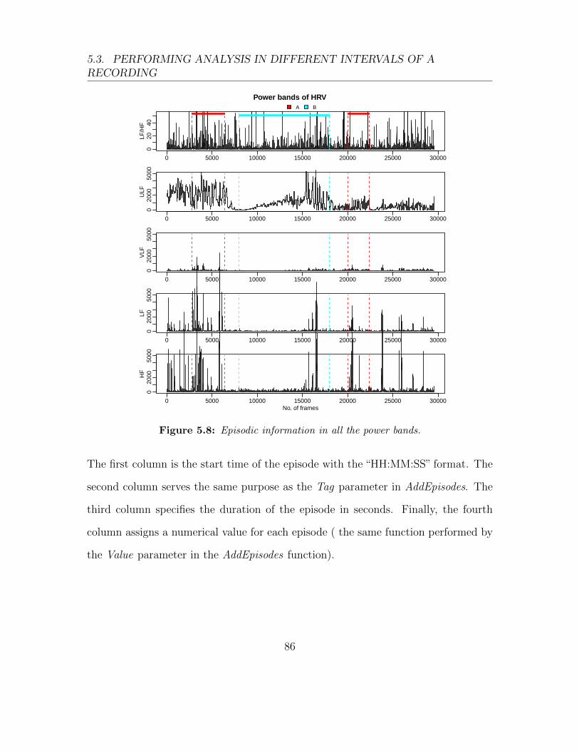
5.3. PERFORMING ANALYSIS IN DIFFERENT INTERVALS OF ARECORDING
0 5000 10000 15000 20000 25000 30000
020
40LF
/HF
A B
0 5000 10000 15000 20000 25000 30000
020
0050
00U
LF
0 5000 10000 15000 20000 25000 30000
020
0050
00V
LF
0 5000 10000 15000 20000 25000 30000
020
0050
00LF
0 5000 10000 15000 20000 25000 30000
020
0050
00
No. of frames
HF
Power bands of HRV
Figure 5.8: Episodic information in all the power bands.
The first column is the start time of the episode with the “HH:MM:SS” format. The
second column serves the same purpose as the Tag parameter in AddEpisodes. The
third column specifies the duration of the episode in seconds. Finally, the fourth
column assigns a numerical value for each episode ( the same function performed by
the Value parameter in the AddEpisodes function).
86

5.3. PERFORMING ANALYSIS IN DIFFERENT INTERVALS OF ARECORDING
It must be taken into account that the LoadEpisodesAscii function skips the first
line of the ASCII file because it assumes that the first line will contain a header (the
format of this header does not really matter). If there is no header line in the file,
the user can specify it to the function using the header parameter (by default, it is
setted to TRUE).
As an example, we are going to create an ASCII file containing the same information
as the episodes “A” and “B” that we programmatically introduced in the AddE-
pisodes(5.3.1) paragraph. We will also add information about a “C” episode that the
LoadEpisodesAscii function will skip. We shall call this file “annotationsFile.txt”.
This file will have the following content:
InitTime Type Duration Value
00:11:40 ”A” 900 1
01:23:20 “A” 600 2
00:33:20 ”B” 2500 3
01:00:00 ”C” 100 4
The LoadEpisodesAscii function takes as input parameters: the absolute path to
the episodes file to be read (FileName), the types of episodes that should be read
(Tag) and the time (“HH:MM:SS”) at which the recording began (InitTime). This
last parameter enables reading those files in which the initial time of episodes was
specified in absolute time, and not relative to the start of the recording. Since we
wrote relative times in the ASCII file, we should use InitTime=“0:0:0”. Thus, in
order to read just the episodes tagged as “A” from our file, we could write:
87

5.3. PERFORMING ANALYSIS IN DIFFERENT INTERVALS OF ARECORDING
> hrv.data = CreateHRVData( )
> hrv.data = LoadBeatAscii(hrv.data,"example.beats","beatsFolder")
> hrv.data = SetVerbose(hrv.data,TRUE)
> hrv.data = LoadEpisodesAscii(hrv.data,Tag=c("A"),InitTime="0:0:0",
+ FileName="beatsFolder/annotationsFile.txt")
** Loading episodes file: beatsFolder/annotationsFile.txt **
Path: .
Tag: A
Initial time: 00:00:0.000
Data includes values associated to episodes
Loaded 2 episodes from file
Number of episodes: 2
5.3.4 LoadApneaWFDB
The LoadApneaWFDB function allows the user to load apnea annotations from a
WFDB file (the user must ensure that there is a file with the .apn extension between
the WFDB recording’s files). The function takes as input parameters the name of
the WFDB file (RecordName), the path to the WFDB file (RecordPath) and a name
for the apnea episodes (Tag, its default value is “APNEA”). The use of this function
requires the installation of the WFDB tools (see chapter 3).
As an illustrative example, we are going to read the apnea episodes for the “a03” file
of the ApneaECG database from PhysioBank (see the Reading files in WFDB format
paragraph). The plot of the non interpolated HR series is shown in Figure 5.9.
88

5.3. PERFORMING ANALYSIS IN DIFFERENT INTERVALS OF ARECORDING
> hrv.wfdb = CreateHRVData()
> hrv.wfdb = SetVerbose(hrv.wfdb, TRUE)
> hrv.wfdb = LoadBeat(hrv.wfdb, fileType = "WFDB", "a03", RecordPath =".",
+ annotator = "qrs")
** Loading beats positions for record: a03 **
Path: .
Opening header file: a03.hea
No time information in header: 00:00:00
No date information in header: 01/01/1900
Date: 01/01/1900
Time: 00:00:00
Number of beats: 34254
> hrv.wfdb = LoadApneaWFDB(hrv.wfdb, RecordName="a03",Tag="Apnea",
+ RecordPath=".")
** Loading apnea episodes for record: a03 **
Path: .
Header info already present for: a03
Command: rdann -r a03 -a apn
Number of labels: 518
** Adding new episodes **
Added 11 episodes from file
Number of episodes: 11
89

5.3. PERFORMING ANALYSIS IN DIFFERENT INTERVALS OF ARECORDING
> hrv.wfdb = BuildNIHR(hrv.wfdb)
** Calculating non-interpolated heart rate **
Number of beats: 34254
> PlotNIHR(hrv.wfdb,Tag="all")
** Plotting non-interpolated instantaneous heart rate **
Number of points: 34254
Episodes in plot: Apnea
No of episodes: 11
No of classes of episodes: 1
5.3.5 Analyzing HRV inside and outside the episodes
RHRV provides basic functionality for comparing data inside and outside each
episode. The simplest function that the user can use for this purpose is the
SplitHRbyEpisodes function, that splits the interpolated heart rate series into two
vectors containing samples inside (the “InEpisodes” vector) and outside the episode
(the “OutEpisodes” vector) specified in the Tag argument. For example, if we want
to compare the HR series inside and outside the apnea episodes from the “a03” file,
we could use:
> # remember to interpolate the Heart Rate series!!
> hrv.wfdb = InterpolateNIHR (hrv.wfdb, freqhr = 4)
90
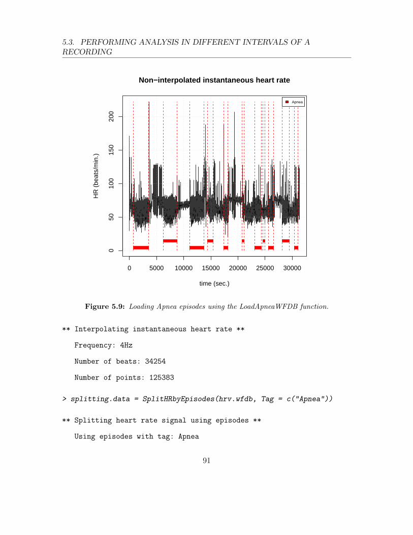
5.3. PERFORMING ANALYSIS IN DIFFERENT INTERVALS OF ARECORDING
0 5000 10000 15000 20000 25000 30000
050
100
150
200
time (sec.)
HR
(be
ats/
min
.)Apnea
Non−interpolated instantaneous heart rate
Figure 5.9: Loading Apnea episodes using the LoadApneaWFDB function.
** Interpolating instantaneous heart rate **
Frequency: 4Hz
Number of beats: 34254
Number of points: 125383
> splitting.data = SplitHRbyEpisodes(hrv.wfdb, Tag = c("Apnea"))
** Splitting heart rate signal using episodes **
Using episodes with tag: Apnea
91

5.3. PERFORMING ANALYSIS IN DIFFERENT INTERVALS OF ARECORDING
Number of episodes: 11
Inside episodes: 58919 points
Outside episodes: 66464 points
It is straightforward to use a statistical function for comparing both vectors. For
example:
> cat("comparing the mean inside and outside Apnea episodes...\n")
comparing the mean inside and outside Apnea episodes...
> cat("Apnea mean: ",mean(splitting.data$InEpisodes),"\n")
Apnea mean: 61.94101
> cat("Normal mean: ",mean(splitting.data$OutEpisodes),"\n")
Normal mean: 69.11033
Although the previous example illustrates how to access the data inside and outside a
certain type of episode, we could have used the AnalyzeHRbyEpisodes for comparing
its means. This function analyzes the heart rate series evaluating the desired function
(func parameter) inside and outside the episodes of interest (Tag parameter). Thus,
we could have executed:
> cat("comparing the mean inside and outside the Apnea episodes...\n")
comparing the mean inside and outside the Apnea episodes...
92
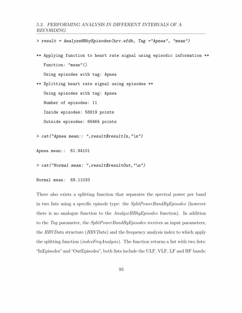
5.3. PERFORMING ANALYSIS IN DIFFERENT INTERVALS OF ARECORDING
> result = AnalyzeHRbyEpisodes(hrv.wfdb, Tag ="Apnea", "mean")
** Applying function to heart rate signal using episodic information **
Function: "mean"()
Using episodes with tag: Apnea
** Splitting heart rate signal using episodes **
Using episodes with tag: Apnea
Number of episodes: 11
Inside episodes: 58919 points
Outside episodes: 66464 points
> cat("Apnea mean:: ",result$resultIn,"\n")
Apnea mean:: 61.94101
> cat("Normal mean: ",result$resultOut,"\n")
Normal mean: 69.11033
There also exists a splitting function that separates the spectral power per band
in two lists using a specific episode type: the SplitPowerBandByEpisodes (however
there is no analogue function to the AnalyzeHRbyEpisodes function). In addition
to the Tag parameter, the SplitPowerBandByEpisodes receives as input parameters,
the HRVData structure (HRVData) and the frequency analysis index to which apply
the splitting function (indexFreqAnalysis). The function returns a list with two lists:
“InEpisodes”and“OutEpisodes”, both lists include the ULF, VLF, LF and HF bands:
93

5.3. PERFORMING ANALYSIS IN DIFFERENT INTERVALS OF ARECORDING
> # ...
> hrv.wfdb = CreateFreqAnalysis(hrv.wfdb)
** Creating frequency analysis
Data has now 1 frequency analysis
> hrv.wfdb = CalculatePowerBand( hrv.wfdb , indexFreqAnalysis= 1,
+ type = "wavelet", wavelet = "la8", bandtolerance = 0.01, relative = FALSE)
** Calculating power per band **
** Using Wavelet analysis **
Power per band calculated
> splitting.data = SplitPowerBandByEpisodes(hrv.wfdb,
+ indexFreqAnalysis = 1, Tag = c("Apnea"))
** Splitting power bands using episodes**
Using episodes with tag: Apnea
Number of episodes: 11
No. of frames: 125383
No. of frames in episodes: 58931
No. of frames outside episodes: 66452
> cat("comparing the mean power in the LF band
+ inside and outside A episodes...\n")
comparing the mean power in the LF band
inside and outside A episodes...
94

5.4. STORING AND READING HRVDATA
> cat("LF power in Apnea episodes: ",
+ mean(splitting.data$InEpisodes$LF),"\n")
LF power in Apnea episodes: 3194.988
> cat("LF power in Normal episodes: ",
+ mean(splitting.data$OutEpisodes$LF),"\n")
LF power in Normal episodes: 811.5181
5.4 Storing and reading HRVData
In order to save interesting results RHRV provides functionality for storing and
reading HRVData structures. For example, if the user wants to store the hrv.wfdb
structure from the previous section, he just has to write:
> WriteToFile(hrv.wfdb, name="HRVstructure")
** Writing file: HRVstructure.hrv
File HRVstructure.hrv already exists
18468167 bytes written
The WriteToFile function will store the HRVData structure in a file called
“HRVstructure.hrv”. Note that the “.hrv” suffix has been added. Additionally,
the user may specify the behaviour of the function if the file already exists with the
overwrite parameter. The default value overwrites existing files. If the user wants
to prevent losing previous data stored in the “HRVstructure.hrv” file, he can write:
95

5.4. STORING AND READING HRVDATA
> WriteToFile(hrv.wfdb, name="HRVstructure", overwrite = FALSE)
Error in WriteToFile(hrv.data, name = "HRVstructure", overwrite = FALSE) :
--- File exists... Not overwriting it!! ---
--- Quitting now!! ---
Note that the function informs about the existence of a previous file named
“HRVstructure.hrv”.
In order to read HRVData structures that had been previously stored, the Read-
FromFile function is provided:
> data = ReadFromFile(name = "HRVstructure", verbose = TRUE)
** Reading file: HRVstructure.hrv
18468167 bytes read
Note that the “.hrv” prefix is not included in the file’s name, although the HRVData
structure was stored as “HRVstructure.hrv”. The user can control the verbosity level
using the verbose argument.
96
Chapter 6
HRV nonlinear analysis
6.1 An introduction to nonlinear analysis tech-
niques
RHRV implements all the nonlinear statistics presented in Section 2.2.3. As we
shall see in the next sections, most of the nonlinear statistics share a common
name convention for their functions: the CalculateX, the EstimateX and the PlotX
functions, being X the name of the statistic (for example corrDim). This naming
convention reflects that these statistics share a similar estimation process: first,
the CalculateX function performs some heavy computations that are required for
obtaining the value of the statistic. The statistic is then obtained as the slope of
a regression involving these computations. The regression is performed with the
EstimateX function. The PlotX function draws the variables involved in the re-
97
6.1. AN INTRODUCTION TO NONLINEAR ANALYSIS TECHNIQUES
gression, which may be useful to check if the statistics follow the expected behaviour.
In order to load the example file that we shall use to illustrate the nonlinear functions
included in RHRV, we may execute:
> library(RHRV)
> hrv.data = CreateHRVData()
> hrv.data = LoadBeatAscii(hrv.data, RecordName="nonlinearHB.beats",
+ RecordPath="beatsFolder")
> hrv.data = BuildNIHR(hrv.data)
> hrv.data = SetVerbose(hrv.data,TRUE)
The beats from this file were generated synthetically from a nonlinear process in
order to show the expected behaviour of a truly nonlinear RR time series and avoid
some issues when dealing with a noisy process. Thus, this file has no physiological
meaning. An example of nonlinear HRV analysis with a real RR series is given in
Section 6.2.
Before performing the nonlinear analysis we must create the data analysis structure
that will store all the results from the analysis: the NonLinearAnalysis list, under
the HRVData structure. Just as with the others analysis structures, each nonlinear
analysis structure is identified by a unique number. To create an analysis structure,
the CreateNonLinearAnalysis function is used.
> hrv.data = CreateNonLinearAnalysis(hrv.data)
98

6.1. AN INTRODUCTION TO NONLINEAR ANALYSIS TECHNIQUES
** Creating non linear analysis
Data has now 1 nonlinear analysis
In the next few sections we shall present the basics for performing the most widely-
used nonlinear analysis algorithms (Although some of the algorithms will not be
presented here, but in Section 6.2). Due to the heterogeneity of the nonlinear algo-
rithms, we will also explain how to access the computations for each algorithm as
they are presented.
6.1.1 Nonlinearity Test
Before applying nonlinear analysis to the RR time series we should ensure that
the HR shows, indeed, some degree of nonlinearity. If we don’t , there is a risk of
obtaining unreliable results. There exist two functions in RHRV that allow running
nonlinearity tests: NonlinearityTests and SurrogateTest.
The NonlinearityTests permits running a wide variety of nonlinearity tests including:
two tests for neglected nonlinearity that are based on neural networks, the Keenan
test for nonlinearity, the McLeod and Li test for nonlinearity and the Tsay’s test.
Surrogate data testing tests the null hypothesis that the data was generated from
a stationary linear stochastic process with Gaussian inputs. Surrogate data testing
consists on generating a surrogate data set showing the same linear properties of
the RR time series. Then, a statistic is calculated for the RR time series and all the
surrogate set. If the value of the statistic is significantly different for the RR series
99
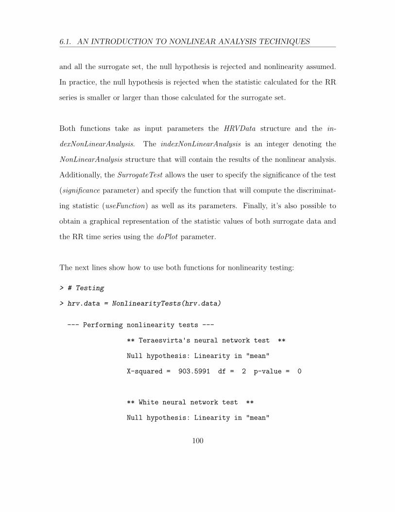
6.1. AN INTRODUCTION TO NONLINEAR ANALYSIS TECHNIQUES
and all the surrogate set, the null hypothesis is rejected and nonlinearity assumed.
In practice, the null hypothesis is rejected when the statistic calculated for the RR
series is smaller or larger than those calculated for the surrogate set.
Both functions take as input parameters the HRVData structure and the in-
dexNonLinearAnalysis. The indexNonLinearAnalysis is an integer denoting the
NonLinearAnalysis structure that will contain the results of the nonlinear analysis.
Additionally, the SurrogateTest allows the user to specify the significance of the test
(significance parameter) and specify the function that will compute the discriminat-
ing statistic (useFunction) as well as its parameters. Finally, it’s also possible to
obtain a graphical representation of the statistic values of both surrogate data and
the RR time series using the doPlot parameter.
The next lines show how to use both functions for nonlinearity testing:
> # Testing
> hrv.data = NonlinearityTests(hrv.data)
--- Performing nonlinearity tests ---
** Teraesvirta's neural network test **
Null hypothesis: Linearity in "mean"
X-squared = 903.5991 df = 2 p-value = 0
** White neural network test **
Null hypothesis: Linearity in "mean"
100

6.1. AN INTRODUCTION TO NONLINEAR ANALYSIS TECHNIQUES
X-squared = 877.33 df = 2 p-value = 0
** Keenan's one-degree test for nonlinearity **
Null hypothesis: The time series follows some AR process
F-stat = 516.1898 p-value = 8.409783e-109
** McLeod-Li test **
Null hypothesis: The time series follows some ARIMA process
Maximum p-value = 0
** Tsay's Test for nonlinearity **
Null hypothesis: The time series follows some AR process
F-stat = 29.45 p-value = 0
** Likelihood ratio test for threshold nonlinearity **
Null hypothesis: The time series follows some AR process
Alternativce hypothesis: The time series follows some TAR process
X-squared = 2600.526 p-value = 0
> hrv.data = SurrogateTest(hrv.data, significance = 0.05,
+ useFunction = timeReversibility, tau=4, doPlot = TRUE)
Computing statistics
Null Hypothesis: Original data comes from a linear stochastic process
Reject Null hypothesis: Original data's statistic is the greatest one
101

6.1. AN INTRODUCTION TO NONLINEAR ANALYSIS TECHNIQUES
0 2000 4000 6000
0.0
0.5
1.0
1.5
2.0
2.5
3.0
Surrogate data testing
Statistic
Surrogate dataOriginal data
Figure 6.1: Surrogate data testing.
The SurrogateTest uses the timeReversibility function from the nonlinearTseries
package. This function implements the third-order statistic
ψ(τ) =1
N − τ
N∑i=τ+1
(sn − sn−τ )3,
that is useful for measuring the asymmetry of a series under time reversal. Since
linear stochastic series are symmetric under time reversal, this statistic may be used
for testing if the data was generated from a stationary linear stochastic process (the
null hypothesis). The tau parameter is a parameter of the timeReversibility function
that sets τ = tau. It must be noted that the discrimination power of the time
102

6.1. AN INTRODUCTION TO NONLINEAR ANALYSIS TECHNIQUES
simmetry test is low. We have use it here for illustrative purposes. Figure 6.1 shows
the results of the surrogate data testing.
6.1.2 Phase space reconstruction
As exposed in Section 2.2.3.1 the Takens embedding theorem provides a method for
phase space reconstruction. However, it does not provide information on how to
select τ and m parameters. Fortunately, the RHRV package provides functionality
for estimating both parameters.
6.1.2.1 Time lag estimation
In practical applications, the τ parameter is firstly selected. Then, the embedding
dimension is estimated for a fixed value of the τ parameter.
The τ parameter can be estimated in RHRV by using the CalculateTimeLag function.
This function selects the time lag based on the following reasoning: if the time lag
used to build the Takens’ vectors is too small, the coordinates will be too highly
temporally correlated and the embedding will tend to cluster around the diagonal in
the phase space. If the time lag is chosen too large, the resulting coordinates may be
almost uncorrelated and the resulting embedding will be very complicated. There is
a wide variety of methods for estimating an appropriate time lag based on the study
of the autocorrelation function of a given time series:
• Select the time lag where the autocorrelation function decays to 0 (first.zero
method).
103

6.1. AN INTRODUCTION TO NONLINEAR ANALYSIS TECHNIQUES
• Select the time lag where the autocorrelation function decays to 1/e
(first.e.decay method).
• Select the time lag where the autocorrelation function reaches its first minimum
(first.minimum method).
• Select the time lag where the autocorrelation function decays to the value
specified by the user (first.value method and value parameter).
The CalculateTimeLag function takes as input parameters the HRVData and the
method, value, lagMax and doPlot parameters. The method parameter indicates the
method that we shall use to estimate the time lag . Its value must be “first.zero”,
“first.e.decay”, “first.minimum” or “first.value”. The value parameter denotes the
value that the autocorrelation function must cross in order to select the time lag
if the “first.value” method is used. The lagMax parameter specifies the maximum
lag at which to calculate the autocorrelation function. By default, the length of the
timeSeries is used. Finally, the logical doPlot parameter indicates if a plot of the
autocorrelation function is shown or not.
In the following example we estimate a proper time lag by using the different methods
explained above:
> # method "first.zero"
> CalculateTimeLag(hrv.data,method="first.zero",lagMax=100)
104
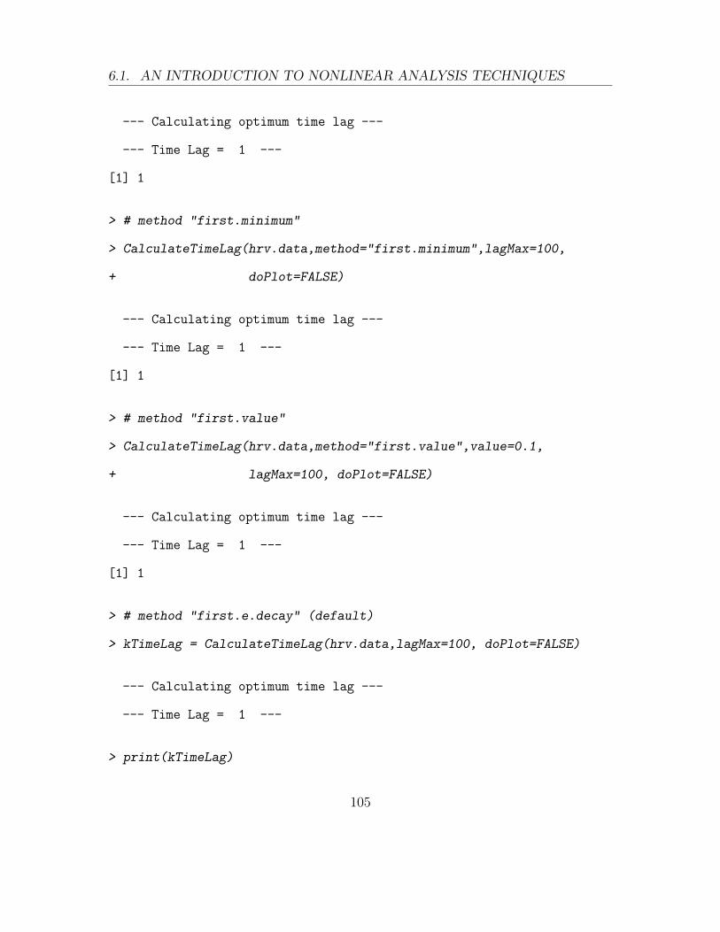
6.1. AN INTRODUCTION TO NONLINEAR ANALYSIS TECHNIQUES
--- Calculating optimum time lag ---
--- Time Lag = 1 ---
[1] 1
> # method "first.minimum"
> CalculateTimeLag(hrv.data,method="first.minimum",lagMax=100,
+ doPlot=FALSE)
--- Calculating optimum time lag ---
--- Time Lag = 1 ---
[1] 1
> # method "first.value"
> CalculateTimeLag(hrv.data,method="first.value",value=0.1,
+ lagMax=100, doPlot=FALSE)
--- Calculating optimum time lag ---
--- Time Lag = 1 ---
[1] 1
> # method "first.e.decay" (default)
> kTimeLag = CalculateTimeLag(hrv.data,lagMax=100, doPlot=FALSE)
--- Calculating optimum time lag ---
--- Time Lag = 1 ---
> print(kTimeLag)
105

6.1. AN INTRODUCTION TO NONLINEAR ANALYSIS TECHNIQUES
[1] 1
Most of the nonlinear algorithms in RHRV accept as input both time lag and
embedding dimension parameters. If they are not specified, RHRV estimates them
by using the functions explained in this section and the next one. However we
strongly recommend to estimate them just once because of computational efficiency.
Thus, we store the kTimeLag parameter to use it in all the examples of this section.
Figure 6.2 shows the autocorrelation function used in the time lag estimation.
0 20 40 60 80 100
−0.
50.
00.
51.
0
Lag
AC
F
Series time.series
Figure 6.2: Autocorrelation function of the niHR time series used for calculate the opti-mum TimeLag.
106
6.1. AN INTRODUCTION TO NONLINEAR ANALYSIS TECHNIQUES
6.1.2.2 Embedding dimension estimation
Once the time lag has been estimated, it is possible to obtain a proper embedding
dimension by using the algorithm explained in [8]. The Cao’s algorithm uses 2
functions in order to estimate the embedding dimension from a time series: the
E1(d) and the E2(d) functions, where d denotes the dimension.
E1(d) stops changing when d is greater than or equal to the embedding dimension
m, staying close to 1. On the other hand, E2(d) is used to distinguish deterministic
signals from stochastic signals. For deterministic signals, there exists some d fulfilling
E2(d) 6= 1. For stochastic signals, E2(d) is approximately 1 for all the values. The
CalculateEmbeddingDim function implements this algorithm in the RHRV package.
The CalculateEmbeddinDim takes as input parameters the HRVData structure, the
number of points of the time series to be used for estimating the embedding di-
mension (numberPoints); the time lag calculated in the previous Section (timeLag);
the maximum possible embedding dimension (maxEmbeddingDim); the threshold
that E1(d) must cross for considering that it is close to the limit value 1 (threshold ;
the default value is 0.95); the maximum relative change in E1(d) with respect to
E1(d − 1) in order to consider that the E1 function has been stabilized and that it
will stop changing (maximumRelativeValue; the default value is 0.01) and the doPlot
parameter (If TRUE a plot of E1(d) and E2(d) is shown).
107

6.1. AN INTRODUCTION TO NONLINEAR ANALYSIS TECHNIQUES
In the following example we estimate a proper embedding dimension using the time
lag calculated in the previous section. Figure 6.3 shows the resulting plot.
> kEmbeddingDim = CalculateEmbeddingDim(hrv.data,
+ numberPoints = 10000,
+ timeLag = kTimeLag,
+ maxEmbeddingDim = 15)
--- Calculating optimum embedding dimension ---
>
2 4 6 8 10 12 14
0.0
0.2
0.4
0.6
0.8
1.0
1.2
Computing the embedding dimension
dimension (d)
E1(
d) &
E2(
d)
E1(d)E2(d)limits for E1(d)
Figure 6.3: Estimation of the embedding dimension using the Cao’s algorithm.
108
6.1. AN INTRODUCTION TO NONLINEAR ANALYSIS TECHNIQUES
We store the result in the kEmbeddingDim variable in order to use it in the remainder
of this section.
6.1.3 Computing nonlinear statistics
6.1.3.1 The classic correlation dimension
In order to calculate the correlation dimension of our RR time series we can use the
CalculateCorrDim function. This function takes as input the HRVData structure
to be analyzed and the index of the NonlinearAnalysis structure that shall store
the results. The embedding dimensions in which the CalculateCorrDim will be
computed are specified with the minEmbeddingDim and the maxEmbeddingDim
parameters (remember that we should compute the correlation dimension for several
embedding dimensions). The time lag needed for reconstructing the phase space is
provided by the timeLag parameter. The minRadius and maxRadius parameters
specify the radius in which the correlation sum is going to be calculated. The
number of points used to compute this radius range can be specified with the
pointsRadius parameter (i.e. we shall use pointsRadius points in order to cover
the [minRadius,maxRadius] interval). The Theiler window is specified using the
theilerWindow parameter. Finally, a log-log plot of the correlation sum Vs. the
radius can be obtained by setting doPlot = TRUE (default).
For analyzing our hrv.data structure we shall use the embedding dimension and
time lag obtained in Section 6.1.2. Thus, we set timeLag = kTimeLag and we se-
109

6.1. AN INTRODUCTION TO NONLINEAR ANALYSIS TECHNIQUES
lect a sequence of dimensions surrounding kEmbeddingDim. For example, we may
use minEmbeddingDim = kEmbeddingDim - 1 and maxEmbeddingDim = kEmbed-
dingDim + 2. In order to select the radius we have to take into account that we
are analyzing RR intervals in milliseconds. Thus, the selection minRadius = 1 and
maxRadius = 100 will probably cover the most important range of the correlation
sum C(r). By selecting pointsRadius = 100, the correlation sum C(r) will be com-
puted in r = 1, 2, .., 100. In order to select a proper Theiler window, the autocor-
relation function may be used. Figure 6.2 shows that the RR series is practically
uncorrelated after the time lag 10. In order to be sure that we got rid of the tempo-
ral correlations we set theilerWindow = 20. Finally, we set doPlot=FALSE (later,
we will plot the correlation sum with the PlotCorrDim function).
> my.index = 1
> hrv.data = CalculateCorrDim(hrv.data,
+ indexNonLinearAnalysis = my.index,
+ minEmbeddingDim = kEmbeddingDim - 1,
+ maxEmbeddingDim = kEmbeddingDim + 2,
+ timeLag = kTimeLag, minRadius=1,
+ maxRadius=100, pointsRadius = 100,
+ theilerWindow = 20, doPlot = FALSE)
--- Computing the Correlation sum ---
As usual, we may use the $ operator from the R language to access the correlation
sum calculated with the CalculateCorrDim function and stored under the correla-
tion$computations field of the NonLinearAnalysis structure:
110

6.1. AN INTRODUCTION TO NONLINEAR ANALYSIS TECHNIQUES
> corr.struct = hrv.data$NonLinearAnalysis[[my.index]]$correlation
> corrSum = corr.struct$computations
Now, in order to access to the corrSum attributes we may write:
> # Let's print the four first rows and columns of the correlation matrix
> print(corrSum$corr.matrix[1:4,1:4])
100 95.4548456661834 91.1162756115489 86.9749002617783
4 0.9988547 0.9917903 0.9854796 0.9778878
5 0.9984679 0.9896422 0.9818793 0.9728309
6 0.9980811 0.9874943 0.9782899 0.9678070
7 0.9972923 0.9849646 0.9743409 0.9624882
> # Access the radius and embedding dimensions used for computations
> radius = corrSum$radius
> embeddingDims = corrSum$embedding.dims
Note the correlation matrix stores all the correlation sums that have been computed.
Each row stores the correlation sum for a concrete embedding dimension whereas
each colum stores the correlation sum for a specific radius. Note that the names
of the matrix dimensions denote the embedding dimension and the radius (in
descending order).
A graphical representation of the correlation sum can be obtained by using the Plot-
CorrDim function. This function shows a log-log plot of the correlation sum Vs the
radius and the local slopes of log10(C(r)) Vs log10(C(r)).
111

6.1. AN INTRODUCTION TO NONLINEAR ANALYSIS TECHNIQUES
> PlotCorrDim(hrv.data,indexNonLinearAnalysis=my.index)
1 2 5 10 20 50 100
1e−
041e
−02
1e+
00Correlation Sum Vs radius
Radius r
Cor
rela
tion
Sum
C(r
)
1 2 5 10 20 50 100
210
5050
0
Local slopes of the Correlation Sum Vs Radius
Radius r
Loca
l slo
pes
of th
e C
orre
latio
n S
um
Embedding dimension
45
67
Figure 6.4: Correlation sums calculation.
In order to get an estimation of the correlation dimension, the EstimateCorrDim
function can be used. This function estimates the correlation dimension of the RR
time series by averaging the slopes of the embedding dimensions specified in the
useEmbeddings parameter. The slopes are determined by performing a linear re-
gression over the radius’ range specified in regressionRange. The user must select
112
6.1. AN INTRODUCTION TO NONLINEAR ANALYSIS TECHNIQUES
the dimensions and radius in which the slopes of the correlation sum are approxi-
mately equal. If such a region does not exist, the estimation should be discarded. In
our case, we may select all the embedding dimensions and set the regressionRange
to [1.5, 10] (see Figure 6.4). If doPlot=TRUE a graphic of the regression over the
data is shown. The results are returned into a new field called statistic under the
hrv.data$NonLinearAnalysis[[indexNonLinearAnalysis]]$correlation list:
> hrv.data = EstimateCorrDim(
+ hrv.data,
+ indexNonLinearAnalysis=my.index,
+ regressionRange=c(1.5,10),
+ useEmbeddings=(kEmbeddingDim-1):(kEmbeddingDim+2),
+ doPlot=TRUE)
--- Estimating the Correlation dimension ---
--- Correlation dimension = 1.828973 ---
> # We may add a legend to the plot
> legend(x=10,y=-3, lty = rep(1,3), col = 1:3,
+ title="Embedding dimension",
+ legend = (kEmbeddingDim-1):(kEmbeddingDim + 2))
> cat("The correlation dimension is ",
+ hrv.data$NonLinearAnalysis[[my.index]]$
+ correlation$statistic,"\n")
The correlation dimension is 1.828973
113
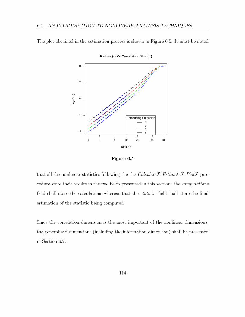
6.1. AN INTRODUCTION TO NONLINEAR ANALYSIS TECHNIQUES
The plot obtained in the estimation process is shown in Figure 6.5. It must be noted
1 2 5 10 20 50 100
−4
−3
−2
−1
0
Radius (r) Vs Correlation Sum (r)
radius r
log(
C(r
))
Embedding dimension
4567
Figure 6.5
that all the nonlinear statistics following the the CalculateX -EstimateX -PlotX pro-
cedure store their results in the two fields presented in this section: the computations
field shall store the calculations whereas that the statistic field shall store the final
estimation of the statistic being computed.
Since the correlation dimension is the most important of the nonlinear dimensions,
the generalized dimensions (including the information dimension) shall be presented
in Section 6.2.
114

6.1. AN INTRODUCTION TO NONLINEAR ANALYSIS TECHNIQUES
6.1.3.2 Sample entropy
In Section 2.2.3.5 we saw that in order to compute the sample entropy of order q
(Hq) of a time series we first have to calculate:
hq(m, r) = log
(Cq(m, r)
Cq(m+ 1, r)
),
and then, we may obtain Hq by taking the limit:
Hq = lim r→0m→∞
hq(m, r).
Thus, in RHRV, in order to use the CalculateSampleEntropy function a “corrDim”
object with several embedding dimensions must exist under the NonLinearAnalysis
structure. Also, the embedding dimensions must be high enough (in order to
“simulate” the limit m→∞).
Let’s compute the sample entropy of our example file. First of all, we shall compute
several correlations sums using high embedding dimensions. In this example, we shall
use at least four times the optimum embedding dimension kEmbeddingDim. Then,
we use the CalculateSampleEntropy function to compute the hq(m, r) function. This
function is quite simple since only takes as input parameters the HRVData being
analyzed, the indexNonLinearAnalysis and the boolean argument doPlot (allowing
to obtain a plot of hq(m, r)).
> hrv.data = CreateNonLinearAnalysis(hrv.data)
115
6.1. AN INTRODUCTION TO NONLINEAR ANALYSIS TECHNIQUES
** Creating non linear analysis
Data has now 2 nonlinear analysis
> my.index = 2
> hrv.data = CalculateCorrDim(hrv.data,
+ indexNonLinearAnalysis = my.index,
+ minEmbeddingDim = 4*kEmbeddingDim,
+ maxEmbeddingDim = 4*kEmbeddingDim+5,
+ timeLag = kTimeLag, minRadius = 1,
+ maxRadius = 100, pointsRadius = 100,
+ theilerWindow = 20, doPlot = FALSE)
--- Computing the Correlation sum ---
> hrv.data = CalculateSampleEntropy(hrv.data,
+ indexNonLinearAnalysis= my.index,
+ doPlot = FALSE)
--- Computing the sample entropy of order 2 ---
We can also plot the hq(m, r) function with the PlotSampleEntropy function. The
resulting figure is shown in Figure 6.6.
> PlotSampleEntropy(hrv.data, indexNonLinearAnalysis=my.index)
Since we require Hq not to depend on m nor r, we shall select a radius range in which
the hq(m, r) is approximately flat. Also, the height of this flat region should be ap-
proximately the same for some embedding dimensions (this height will be the value
116

6.1. AN INTRODUCTION TO NONLINEAR ANALYSIS TECHNIQUES
0 20 40 60 80 100
0.0
0.1
0.2
0.3
0.4
0.5
Sample entropy (q = $(x, entr.order))h$(x, entr.order)(ε)
ln(ε)
h q(ε
)
Embedding dimension
2021
2223
24
Figure 6.6: Sample entropy computations.
of Hq). The EstimateSampleEntropy function takes as input the radius range (re-
gressionRange) and the embedding dimensions selected (useEmbeddings) to compute
an estimation of the sample entropy Hq.
> hrv.data = EstimateSampleEntropy(hrv.data,
+ indexNonLinearAnalysis=my.index,
+ regressionRange=c(10,20),
+ useEmbeddings = 20:22,
+ doPlot = TRUE)
--- Computing the sample entropy---
--- Sample entropy with its order: ---
117

6.1. AN INTRODUCTION TO NONLINEAR ANALYSIS TECHNIQUES
20 21 22
0.2930925 0.2975794 0.3095050
Figure 6.7 shows the plot generated by the EstimateSampleEntropy function.
The results of the sample entropy estimations are stored under the sampleEntropy
field of the NonLinearAnalysis structure as expected: The calculations field stores
hq(m, r) whereas that the statistic field stores the estimate of the sample entropy.
The attributes of the calculations field can be accessed as usual using $. calcula-
tions$sample.entropy returns a matrix containing the hq(m, r) function (the rows
store the computations for an specific embedding whereas that the columns depend
on the radius. calculations$radius and calculations$embedding.dims return the radius
and the embedding dimensions used for calculations:
> se = hrv.data$NonLinearAnalysis[[my.index]]$
+ sampleEntropy$calculations
> # obtaining the h_q(m,r) function, the radius and the embedding dimensions
> sample.function = se$sample.entropy
> radius = se$radius
> dims = se$embedding.dims
> # obtaining the sample entropy estimation
> estimation =
+ hrv.data$NonLinearAnalysis[[my.index]]$sampleEntropy$statistic
> cat("The sample entropy is ")
118
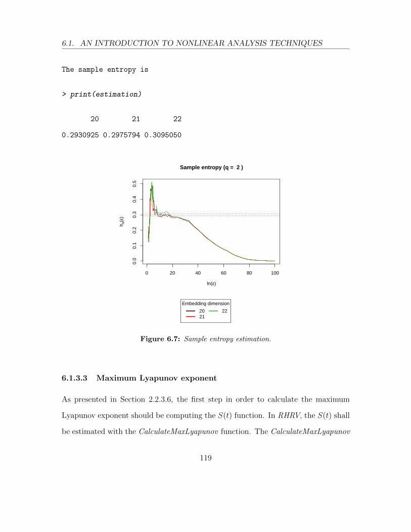
6.1. AN INTRODUCTION TO NONLINEAR ANALYSIS TECHNIQUES
The sample entropy is
> print(estimation)
20 21 22
0.2930925 0.2975794 0.3095050
0 20 40 60 80 100
0.0
0.1
0.2
0.3
0.4
0.5
Sample entropy (q = 2 )
ln(ε)
h q(ε
)
Embedding dimension
2021
22
Figure 6.7: Sample entropy estimation.
6.1.3.3 Maximum Lyapunov exponent
As presented in Section 2.2.3.6, the first step in order to calculate the maximum
Lyapunov exponent should be computing the S(t) function. In RHRV, the S(t) shall
be estimated with the CalculateMaxLyapunov function. The CalculateMaxLyapunov
119

6.1. AN INTRODUCTION TO NONLINEAR ANALYSIS TECHNIQUES
function will average the divergence of several reference points in a m-dimensional
space. The minEmbeddingDim, maxEmbeddingDim and timeLag specify the pa-
rameters for the phase space reconstruction. The number of reference points that
the routine will try to use in order to compute the divergence is specified with
the minRefPoints parameter. A point in the phase space is considered to be a
reference point if there exist a minimum number of close neighbours. 500 points are
usually enough (default). The number of close neighbours needed to be considered a
reference point can be specified with the minNeighs parameter (default value is 5).
The radius specifies the maximum distance in which the routine will look for close
neighbours. Since we are working with the RR time series, a radius in the radius’
range [1− 10] ms seems a proper choice for selecting very close phase space points.
In order to compute the maximal Lyapunov exponent for our example file we could
write:
> my.index = 1
> hrv.data = CalculateMaxLyapunov(
+ hrv.data,
+ indexNonLinearAnalysis = my.index,
+ minEmbeddingDim= kEmbeddingDim,
+ maxEmbeddingDim= kEmbeddingDim+2,
+ timeLag = kTimeLag,
120

6.1. AN INTRODUCTION TO NONLINEAR ANALYSIS TECHNIQUES
+ radius = 3, theilerWindow = 20,
+ doPlot = FALSE)
--- Computing the divergence of the time series ---
As usual, the user should plot S(t) Vs t when looking for the maximal Lyapunov ex-
ponent. This can be done using the doPlot parameter of the CalculateMaxLyapunov
routine or using the PlotMaxLyapunov function.
> PlotMaxLyapunov(hrv.data, indexNonLinearAnalysis = 1)
The resulting plot is shown in Figure 6.8. After plotting the S(t) function we should
check if S(t) shows a linear behaviour for some temporal range. If that’s the case,
its slope is an estimate of the maximal Lyapunov exponent per unit of time. The
EstimateMaxLyapunov routine allows the user to get always an estimate of the
maximal Lyapunov exponent, but the user must check that there is a linear region
in the S(t) Vs t. If such a region does not exist, the estimation should be discarded.
In our example we found a strong linear region in the [1, 6] interval. The regression
performed by the EstimateMaxLyapunov is shown in Figure 6.9.
> hrv.data = EstimateMaxLyapunov(
+ hrv.data,
+ indexNonLinearAnalysis = my.index,
+ regressionRange = c(1,6),
+ useEmbeddings = (kEmbeddingDim):(kEmbeddingDim+2),
+ doPlot = TRUE)
121
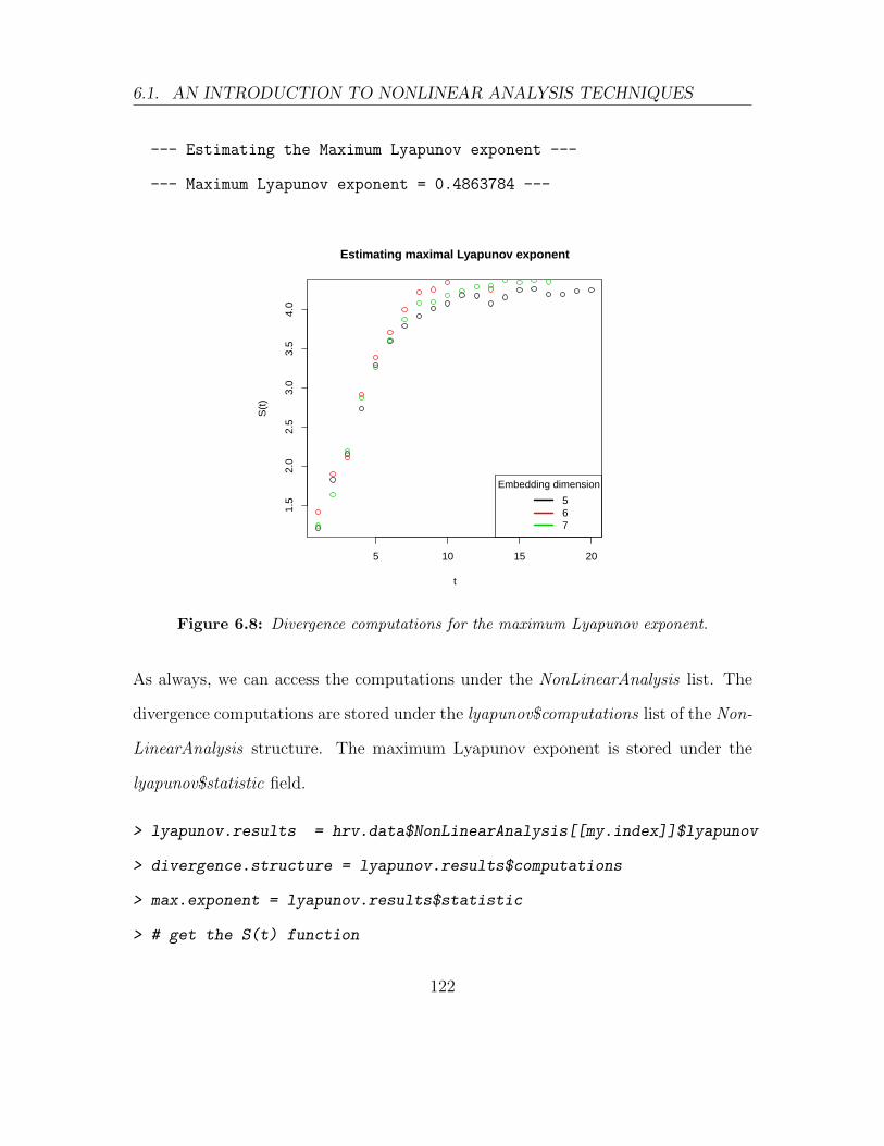
6.1. AN INTRODUCTION TO NONLINEAR ANALYSIS TECHNIQUES
--- Estimating the Maximum Lyapunov exponent ---
--- Maximum Lyapunov exponent = 0.4863784 ---
5 10 15 20
1.5
2.0
2.5
3.0
3.5
4.0
Estimating maximal Lyapunov exponent
t
S(t
)
Embedding dimension
567
Figure 6.8: Divergence computations for the maximum Lyapunov exponent.
As always, we can access the computations under the NonLinearAnalysis list. The
divergence computations are stored under the lyapunov$computations list of the Non-
LinearAnalysis structure. The maximum Lyapunov exponent is stored under the
lyapunov$statistic field.
> lyapunov.results = hrv.data$NonLinearAnalysis[[my.index]]$lyapunov
> divergence.structure = lyapunov.results$computations
> max.exponent = lyapunov.results$statistic
> # get the S(t) function
122

6.1. AN INTRODUCTION TO NONLINEAR ANALYSIS TECHNIQUES
0 5 10 15 20
01
23
4
Estimating maximal Lyapunov exponent
t
S(t
)
Embedding dimension
567
Figure 6.9: Maximum Lyapunov exponent estimation.
> div = divergence.structure$s.function
> tim = divergence.structure$time
> cat("The Max Lyapunov exponent is ",max.exponent,"\n")
The Max Lyapunov exponent is 0.4863784
6.1.3.4 Detrended Fluctuation Analysis
Before introducing the RHRV functionality for performing DFA, we have to review
the DFA procedure presented in Section 2.2.3.7.
1. Integrate the time series to be analyzed. The time series resulting from the
integration will be referred to as the profile.
123

6.1. AN INTRODUCTION TO NONLINEAR ANALYSIS TECHNIQUES
2. Divide the profile into N non-overlapping segments.
3. Calculate the local trend for each of the segments using least-square regression.
Compute the total error for each of the segments.
4. Compute the average of the total error over all segments and take its root
square. By repeating the previous steps for several segment sizes (let’s denote
it by t: number of beats), we obtain the so-called fluctuation function F (t).
5. If the data presents long-range power law correlations: F (t) ∝ tα, we can
estimate the exponent using regression.
6. Usually, when plotting log(F (t)) Vs log(t) we may distinguish two linear re-
gions. By performing a regression on each of them separately, we obtain two
scaling exponents, α1 (the exponent for small values of t, characterizing short-
term fluctuations) and α2 (the exponent for large values of t, characterizing
long-term fluctuations).
Steps 1-4 are performed in RHRV using the CalculateDFA function. In order to
obtain a estimate of some scaling exponent, the user must use the EstimateDFA
function specifying the regression range (window sizes used to detrend the series).
α1 is usually obtained by performing the regression in the 4 ≤ t ≤ 16 range whereas
that α2 is obtained in the 16 ≤ t ≤ 64 range (However the F(t) function must be
linear in these ranges to obtain reliable results).
Besides the HRVData, indexNonLinearAnalysis and doPlot parameters, the Calcu-
lateDFA function accepts as inputs the range of values for the window sizes that will
124

6.1. AN INTRODUCTION TO NONLINEAR ANALYSIS TECHNIQUES
be used to estimate the fluctuation function (windowSizeRange, the default value is
c(10,300)) and the number of different window sizes in that range that will be used
to estimate the Fluctuation function (npoints). The EstimateDFA and PlotDFA
functions work as usual.
> hrv.data = CalculateDFA(hrv.data,
+ indexNonLinearAnalysis = 1,
+ windowSizeRange = c(6, 300),
+ npoints = 25,
+ doPlot = FALSE)
--- Performing Detrended Fluctuation Analysis---
> hrv.data = EstimateDFA(hrv.data,
+ indexNonLinearAnalysis = 1,
+ regressionRange = c(20,100), doPlot = TRUE)
--- Estimating Scaling exponent ---
--- Scaling Exponent number 1 = 0.1442544 ---
Figure 6.10 show the regression performed over the Fluctuation function.
The dfa computations are stored in the dfa$computations list under the NonLin-
earAnalysis structure. The fluctuation function and the windows used for the
computations can be obtained using$fluctuation.function and $window.sizes on the
dfa$computations list, respectively. All the estimated exponents are stored under
125

6.1. AN INTRODUCTION TO NONLINEAR ANALYSIS TECHNIQUES
10 20 50 100 200
1.4
1.6
1.8
2.0
2.2
2.4
Detrended fluctuation analysis
Window size: t
Flu
ctua
tion
func
tion:
F(t
)
Scaling exponent estimate = 0.14
Figure 6.10: DFA.
the NonLinearAnalysis[[index]]$dfa$statistic list. It must be noted that, in this case,
the statistic field may contain more than just one value for the statistic (depending
on the regression range used).
> #obtaining the object pf class "dfa"
> dfa.object = hrv.data$NonLinearAnalysis[[1]]$dfa$computations
> windows = dfa.object$window.sizes
> fluctuation.f = dfa.object$fluctuation.function
> # get the exponent. Note the index 1 in the statistic field!!
> scaling.exp = hrv.data$NonLinearAnalysis[[1]]$dfa$statistic[[1]]
> print(scaling.exp)
126
6.1. AN INTRODUCTION TO NONLINEAR ANALYSIS TECHNIQUES
$range
[1] 20 100
$estimate
[1] 0.1442544
6.1.3.5 Recurrence Quantification Analysis
In order to perform Recurrence Quantification analysis of the RR time series
RHRV provides the RQA routine. The RQA function accepts as parameters the
HRVData, indexNonLinearAnalysis, embeddingDim, timeLag and doPlot with their
usual meaning. The user may also specify the radius (maximum distance between
two phase-space points to be considered a recurrence) and numberPoints (number
of points to be used in the RQA computation). Since this method requires heavy
computations, this last parameter is specially useful.
Let’s apply the RQA function to our example:
> hrv.data = RQA(hrv.data, indexNonLinearAnalysis = my.index,
+ embeddingDim=kEmbeddingDim, timeLag = kTimeLag,
+ radius = 2, doPlot=TRUE)
--- Plotting recurrence plot ---
> # let's see which statistics have been computed...
> names(hrv.data$NonLinearAnalysis[[1]]$rqa)
127

6.1. AN INTRODUCTION TO NONLINEAR ANALYSIS TECHNIQUES
[1] "REC" "RATIO" "DET"
[4] "DIV" "Lmax" "Lmean"
[7] "LmeanWithoutMain" "ENTR" "TREND"
[10] "LAM" "Vmax" "Vmean"
[13] "diagonalHistogram" "recurrenceRate"
> #... and access one of them
> cat("Entropy of the diagonal lines: ",
+ hrv.data$NonLinearAnalysis[[1]]$rqa$ENTR,
+ "\n")
Entropy of the diagonal lines: 1.805314
Figure 6.11 shows the resulting recurrence plot. The only issue of the previous
example is the selection of the radius... Why did we set radius=2 ? Since we are
analyzing RR time series in milliseconds it seems that a reasonable choice for ana-
lyzing close phase space points could be our selection: RR vectors whose maximum
difference is less than 2 ms. However, other similar values for the radius can be used.
An useful rule of thumb for selecting the radius parameter is choosing the radius
so that the recurrence matrix is sparse although it must contain certain vertical or
diagonal lines (deterministic structures). It must also be noted that high values for
the radius may result in very heavy computations.
As seen in the previous example, in addition to the usual statistics (presented in
table 2.1), the RQA function also returns the histogram of the length of diagonal
128

6.1. AN INTRODUCTION TO NONLINEAR ANALYSIS TECHNIQUES
Dimensions: 997 x 997Number of Takens' vector
Num
ber
of T
aken
s' v
ecto
r
200
400
600
800
200 400 600 800
Figure 6.11: Recurrence plot.
lines (diagonalHistogram) and the number of recurrence points among all possible
points depending on the distance to the main diagonal (recurrenceRate). Let’s get a
plot of the recurrence rate (see Figure 6.12):
> recurrence.rate = hrv.data$NonLinearAnalysis[[1]]$rqa$recurrenceRate
> plot(1:length(recurrence.rate),recurrence.rate,type="l",
+ xlab="Distance to main diagonal",ylab="Recurrence Rate",
+ main="Recurrence Rate")
Note the border effects in the plot. Since near the borders there are very few points,
the recurrence rate is usually biased. Of course we can ignore the end of the plot, but
we could have avoided the border effects by using the distanceToBorder parameter
129

6.1. AN INTRODUCTION TO NONLINEAR ANALYSIS TECHNIQUES
0 1000 2000 3000 4000 5000
0.00
0.05
0.10
0.15
Recurrence Rate
Distance to main diagonal
Rec
urre
nce
Rat
e
Figure 6.12: Recurrence plot.
(The points that are closer than distanceToBorder to the border of the recurrence
matrix are ignored when computing the RQA parameters).
The histogram of the length of diagonal lines is not widely used because short diago-
nals prevail. The lmin parameter can be used in order to set a minimum length of a
diagonal line to be considered in the RQA (default value is lmin = 2). Similarly, the
vmin parameter can be used in order to set the minimum length of a vertical line to
be considered in the RQA (default value is vmin = 2 ).
130

6.2. ADVANCED NONLINEAR ANALYSIS TECHNIQUES
6.2 Advanced nonlinear analysis techniques
All the nonlinear functions presented in 6.1 used as example file an RR time series
generated synthetically from a nonlinear process. In this section we will deal with a
real RR time series and we will present all the remaining nonlinear functions.
The example file “example2.beats” that we shall use in the next sections can be
downloaded from the project’s website http://rhrv.r-forge.r-project.org/. The file
was obtained from an ECG of one of the authors of the RHRV package and thus we
expect the file to be from a healthy subject!
> hrv.data = CreateHRVData( )
> hrv.data = LoadBeatAscii(hrv.data,
+ RecordName="example2.beats",
+ RecordPath="beatsFolder")
> hrv.data = BuildNIHR(hrv.data)
> hrv.data = FilterNIHR(hrv.data)
> hrv.data = InterpolateNIHR (hrv.data, freqhr = 4)
> hrv.data = CreateNonLinearAnalysis(hrv.data)
> hrv.data = SetVerbose(hrv.data,TRUE)
First of all, we should run the nonlinearity tests in order to make sure that the time
series shows some degree of nonlinearity. We leave the test to the reader. Now, we
shall estimate both time lag and embedding dimension parameters of our new RR
time series. As always, we first estimate the time lag. The autocorrelation function
131

6.2. ADVANCED NONLINEAR ANALYSIS TECHNIQUES
used for the selection of the time lag is shown in Figure 6.13. This figure also suggest
that a suitable choice for the Theiler window could be ≈ 200.
> kTimeLag = CalculateTimeLag(hrv.data, method = "first.minimum",
+ lagMax = 300)
--- Calculating optimum time lag ---
--- Time Lag = 2 ---
0 50 100 150 200 250 300
0.0
0.2
0.4
0.6
0.8
1.0
Lag
AC
F
Series time.series
Figure 6.13: Autocorrelation function for the RR time series.
We can appreciate that there is high autocorrelation in the time series even for large
time lag values. Although our estimation is reasonable it may happen that some RR
series have their “optimum” time lag at 100 or even more. However, in most HRV
132

6.2. ADVANCED NONLINEAR ANALYSIS TECHNIQUES
publications, the time lag value is not usually selected above 10 or 15.
Now, we may try to obtain an estimation of the embedding dimension (see Figure
6.14). The optimum embedding dimension is 12.
> kEmbeddingDim = CalculateEmbeddingDim(hrv.data,
+ numberPoints = 10000,
+ timeLag = kTimeLag,
+ maxEmbeddingDim = 18)
--- Calculating optimum embedding dimension ---
5 10 15
0.0
0.2
0.4
0.6
0.8
1.0
1.2
Computing the embedding dimension
dimension (d)
E1(
d) &
E2(
d)
E1(d)E2(d)limits for E1(d)
Figure 6.14: Automatic estimation of the embedding dimension.
133

6.2. ADVANCED NONLINEAR ANALYSIS TECHNIQUES
6.2.1 Nonlinear noise reduction
Since the RR intervals are derived from an ECG, the RR time series may suffer
from discretization problems. If the ECG was discretized very coarsely, many RR
intervals shall have the same value. Thus, there will be several identical points in
phase space, which may bias the nonlinear algorithms. RHRV provides functionality
that addresses those situations in which the ECG was discretized very coarsely. In
order to deal with the discretization problem of the RR time series, RHRV provides
the NonLinearNoiseReduction function. This function adds uniform white noise of
a magnitude equal to the resolution of the RR intervals. If the ECG from which
the RR intervals were derived was sampled at fs Hz, uniform [−0.5, 0.5]/fs white
noise is added. Then, a nonlinear noise reduction algorithm is applied. The noise
reduction algorithm performs noise reduction by averaging each Takens’ vector in
an m-dimensional space with his neighbours (time lag=1). Each neighbourhood is
specified with balls of a given radius (max norm is used). Although this procedure
will certainly not solve the discretization problem, it will alleviate it:
> hrv.data = NonLinearNoiseReduction(hrv.data,
+ embeddingDim = kEmbeddingDim)
** Denoising RR time series using nonlinear techniques **
** Calculating non-interpolated heart rate **
Number of beats: 2434
134

6.2. ADVANCED NONLINEAR ANALYSIS TECHNIQUES
Additional parameters for the NonLinearNoiseReduction function are ECGsam-
plingFreq : the ECG sampling frequency (optional, but it can improve the perfor-
mance of the algorithm if provided) and radius : the radius used to looking for
neighbours in the phase space.
6.2.2 Generalized correlation dimensions
Section 6.1.3.1 presented the CalculateCorrDim, EstimateCorrDim and PlotCor-
rDim functions for computing the correlation dimension of an RR time series. These
functions can also be used for computing the generalized correlation dimension. The
user only has to specify the order of the correlation dimension with the corrOrder
parameter in the CalculateCorrDim (the default value is 2, the correlation dimen-
sion). The order must fulfill corrOrder > 1. The generalized correlation dimension
of order q = 1 is known as the information dimension, that is computed with the
CalculateInfDim function (see Section 6.2.3).
As a quick example, we will try to calculate the correlation dimension of order 4 for
our new hrv.data. Figures 6.15 and 6.16 shows the results of the correlation sum
computation and the estimation, respectively.
> hrv.data = CreateNonLinearAnalysis(hrv.data)
** Creating non linear analysis
Data has now 2 nonlinear analysis
135

6.2. ADVANCED NONLINEAR ANALYSIS TECHNIQUES
> my.index = 1
> hrv.data = CalculateCorrDim(hrv.data,
+ indexNonLinearAnalysis = my.index,
+ minEmbeddingDim = kEmbeddingDim - 2,
+ maxEmbeddingDim = kEmbeddingDim + 2,
+ timeLag = kTimeLag, minRadius = 1,
+ maxRadius = 200, pointsRadius = 100,
+ theilerWindow = 200, doPlot = TRUE,
+ corrOrder = 4)
--- Computing the generalized Correlation sum of order 4 ---
> hrv.data = EstimateCorrDim(hrv.data, indexNonLinearAnalysis = 1,
+ regressionRange=c(3*10^5,9*10^5),
+ useEmbeddings = 13:14)
--- Estimating the generalized Correlation dimension of order 4 ---
--- Generalized Correlation dimension of order 4 = 8.585802 ---
>
6.2.3 Information dimension
As seen in Section 2.2.3.4 the information dimension is a particular case of the gen-
eralized correlation dimension when setting the order q = 1. In the RHRV package,
136

6.2. ADVANCED NONLINEAR ANALYSIS TECHNIQUES
1e+05 2e+05 5e+05 1e+06 2e+06 5e+06
1e−
121e
−04
1e+
04
Correlation Sum Vs radius
Radius r^3
Cor
rela
tion
Sum
C(r
)
1e+05 2e+05 5e+05 1e+06 2e+06 5e+06
1e+
011e
+09
1e+
17
Local slopes of the Correlation Sum Vs Radius
Radius r^3
Loca
l slo
pes
of th
e C
orre
latio
n S
um
Embedding dimension
1011
1213
14
Figure 6.15: Generalized correlation dimension computations.
the information dimension is computed using the CalculateInfDim, EstimateInfDim
and PlotInfDim.
Since the EstimateInfDim and PlotInfDim are analogous to the EstimateCorrDim
and PlotCorrDim functions, we shall only review the CalculateInfDim function.
137

6.2. ADVANCED NONLINEAR ANALYSIS TECHNIQUES
1e+05 2e+05 5e+05 1e+06 2e+06 5e+06
−10
−5
0
Radius (r) Vs Correlation Sum (r)
radius r
log(
C(r
))
Figure 6.16: Generalized correlation dimension estimation.
In Section 2.2.3.4 we introduced the method for estimating the information dimen-
sion in practical applications. This algorithm looks for the scaling behaviour of the
average radius that contains a given portion (a ”fixed-mass”) of the total points in
the phase space. By performing a linear regression of log(p) V s. log(< r >) (being
p the fixed-mass of the total points), an estimate of the information dimension (D1)
is obtained.
It must be noted that the calculations for the information dimension are heavier
than those needed for the correlation dimension. However, the user should run the
method for different embedding dimensions to check if D1 saturates.
138

6.2. ADVANCED NONLINEAR ANALYSIS TECHNIQUES
> my.index = 1
> hrv.data = CalculateInfDim(hrv.data,
+ indexNonLinearAnalysis=my.index,
+ minEmbeddingDim=kEmbeddingDim-1,
+ maxEmbeddingDim=kEmbeddingDim+1,
+ timeLag=kTimeLag,
+ minFixedMass=2*10^-3,maxFixedMass=0.25,
+ numberFixedMassPoints=10,
+ radius=0.8,increasingRadiusFactor=1.05,
+ numberPoints=500, theilerWindow=200,
+ doPlot=TRUE)
--- Computing the Information dimension ---
Figure 6.17 shows < log p(r) > Vs. log(r) as obtained from the CalculateInfDim
function. As usual, we may use the Estimate function (EstimateInfDim function) in
order to obtain the estimation and then accessing it using $ under the statistic field.
> hrv.data = EstimateInfDim(hrv.data,
+ indexNonLinearAnalysis=my.index,
+ regressionRange=c(0.0025,0.100),
+ useEmbeddings = (kEmbeddingDim-1):(kEmbeddingDim+1),
+ doPlot=TRUE)
139

6.2. ADVANCED NONLINEAR ANALYSIS TECHNIQUES
0.002 0.005 0.010 0.020 0.050 0.100 0.200
−1
01
2
Information Dimension
fixed mass (p)
<lo
g10(
radi
us)>
0.005 0.010 0.020 0.050 0.100
02
46
8
Local slopes for the Information dimension estimate
fixed mass p
loca
l slo
pe d
1(p)
b b b b b b b bb b b b b b b b
Embedding dimension
1112
13
Figure 6.17: Information dimension computations in RHRV.
--- Estimating the information dimension ---
--- Information dimension = 6.945107 ---
> # Let's print again the value of the information dimension!
> cat("The information dimension is ",
+ hrv.data$NonLinearAnalysis[[my.index]]$infDim$statistic,"\n")
The information dimension is 6.945107
140

6.2. ADVANCED NONLINEAR ANALYSIS TECHNIQUES
Figure 6.18 shows the regression performed for obtaining the estimate of the infor-
mation dimension.
0.002 0.005 0.010 0.020 0.050 0.100 0.200
−1
01
2
Information Dimension
fixed mass (p)
<lo
g10(
radi
us)>
Embedding dimension
111213
Figure 6.18: Information dimension estimation.
6.2.4 Poincare Plot
The PoincarePlot function implements all the functionality for performing Poincare
plot analysis, whether you employ the “classic” calculation methods or those based
on confidence regions (see Section 2.2.3.9).
141

6.2. ADVANCED NONLINEAR ANALYSIS TECHNIQUES
In order to compute the “classic”SD1 and SD2 parameters in the Poincare plot, the
most important arguments of the RHRV routine are the timeLag (τ , that must be
setted to 1) and doPlot (if TRUE, the Poincare plot is shown). The following lines
illustrate the use of this function. The resulting Poincare plot is shown in Figure 6.19.
> # Set timeLag = 1 to obtain the "classic" Poincare parameters
> hrv.data = PoincarePlot(hrv.data,
+ indexNonLinearAnalysis=1,
+ timeLag=1, doPlot=TRUE)
--- Calculating SD1 and SD2 parameters ---
--- Creating Poincare Plot with time lag = 1 ---
--- SD1 = 3.284373 ---
--- SD2 = 7.931162 ---
Figure 6.19 shows the resulting Poincare plot. RHRV also provides functionality for
fitting the ellipse (and computing both SD1 and SD2 parameters) using the theory
of the confidence regions. In order to enable the confidence region estimation the
user can set confidenceEstimation = TRUE. The confidence level can be selected
with the confidence parameter (default value is 0.95). It must be noted that when
timeLag > 1, the confidence region approach is always used.
Figure 6.20 shows the result of applying the following piece of code:
> hrv.data = CreateNonLinearAnalysis(hrv.data)
142

6.2. ADVANCED NONLINEAR ANALYSIS TECHNIQUES
50 60 70 80
5060
7080
Poincare plot
RR[n]
RR
[n+
1]
SD1SD2
Figure 6.19: “Classic” Poincare Plot.
** Creating non linear analysis
Data has now 3 nonlinear analysis
> hrv.data = PoincarePlot(hrv.data,
+ indexNonLinearAnalysis=2,
+ timeLag=1, confidenceEstimation = TRUE,
143

6.2. ADVANCED NONLINEAR ANALYSIS TECHNIQUES
+ confidence = 0.9,
+ doPlot=TRUE)
--- Calculating SD1 and SD2 parameters ---
--- Creating Poincare Plot with time lag = 1 ---
--- SD1 = 7.048153 ---
--- SD2 = 17.01799 ---
The SD1 and SD2 parameters are stored under the PoincarePlot list of the NonLin-
earAnalysis. Of coruse, they can be accessed as usual:
> # results of the first fit ...
> print(hrv.data$NonLinearAnalysis[[1]]$PoincarePlot)
$SD1
[1] 3.284373
$SD2
[1] 7.931162
> # ... vs results of the second one
> print(hrv.data$NonLinearAnalysis[[2]]$PoincarePlot)
$SD1
[1] 7.048153
$SD2
[1] 17.01799
144
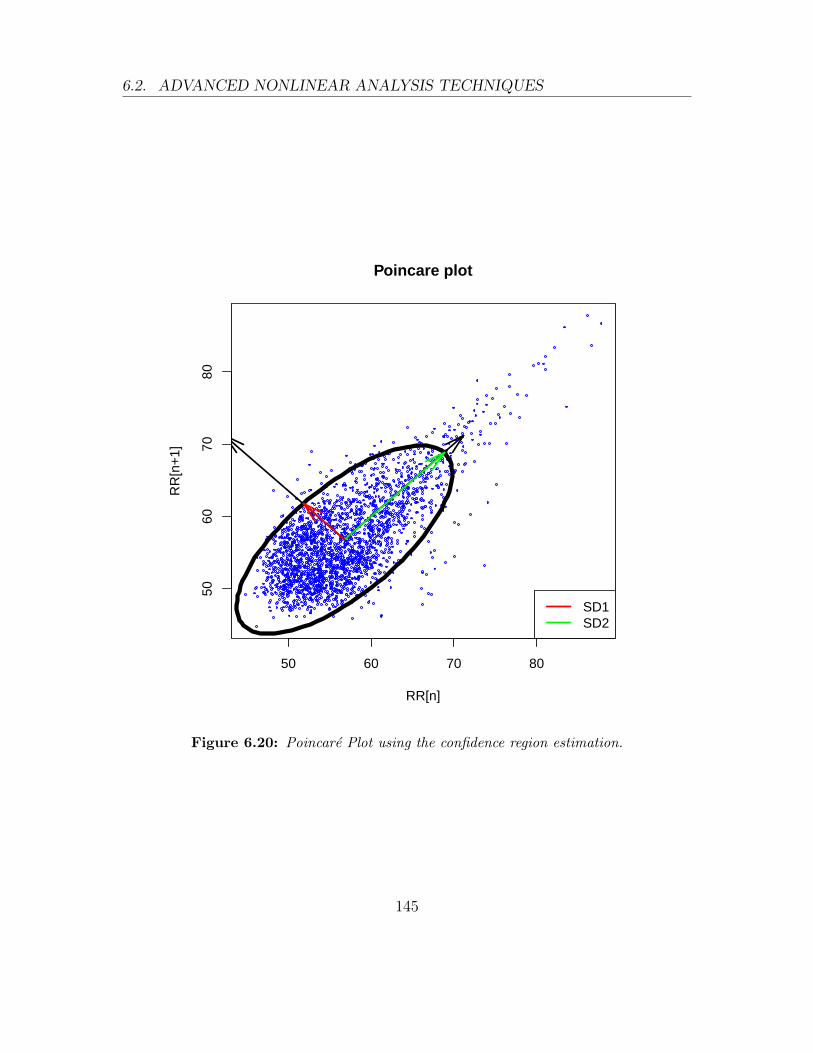
6.2. ADVANCED NONLINEAR ANALYSIS TECHNIQUES
50 60 70 80
5060
7080
Poincare plot
RR[n]
RR
[n+
1]
SD1SD2
Figure 6.20: Poincare Plot using the confidence region estimation.
145

Bibliography
[1] Autonomic nervous system,http://www.scholarpedia.org/article/Autonomic nervous system.
[2] The comprehensive R archive network. http://cran.r-project.org/.
[3] The R project for statistical computing. http://www.r-project.org/.
[4] S. Akselrod, D. Gordon, F.A. Ubel, D.C. Shannon, A.C. Berger, and R.J. Cohen.Power spectrum analysis of heart rate fluctuation: a quantitative probe of beat-to-beat cardiovascular control. Science, 213(4504):220, 1981.
[5] M.L. Appel, R.D. Berger, J.P. Saul, J.M. Smith, and R.J. Cohen. Beat to beatvariability in cardiovascular variables: noise or music? Journal of the AmericanCollege of Cardiology, 14(5):1139–1148, 1989.
[6] R.D. Berger, S. Akselrod, D. Gordon, and R.J. Cohen. An efficient algorithmfor spectral analysis of heart rate variability. Biomedical Engineering, IEEETransactions on, (9):900–904, 1986.
[7] G.G. Berntson. Heart rate variability: Origins, methods and interpretivecaveats. Psychophysiology, 34:623–648, 1997.
[8] Liangyue Cao. Practical method for determining the minimum embedding di-mension of a scalar time series. Physica D: Nonlinear Phenomena, 110(1):43–50,1997.
[9] T. Force. Heart rate variability: standards of measurement, physiological in-terpretation and clinical use. task force of the european society of cardiologyand the north american society of pacing and electrophysiology. Circulation,93(5):1043–65, 1996.
146

BIBLIOGRAPHY
[10] R. Furlan, S. Guzzetti, W. Crivellaro, S. Dassi, M. Tinelli, G. Baselli, S. Cerutti,F. Lombardi, M. Pagani, and A. Malliani. Continuous 24-hour assessment of theneural regulation of systemic arterial pressure and rr variabilities in ambulantsubjects. Circulation, 81(2):537–547, 1990.
[11] D. Gabor. Theory of communication. Electrical Engineers-Part III: Radioand Communication Engineering, Journal of the Institution of, 93(26):429–441,1946.
[12] C.A. Garcıa, A. Otero, X.A. Vila, and M.J. Lado. An open source tool for heartrate variability wavelet-based spectral analysis. In International Joint Confer-ence on Biomedical Engineering Systems and Technologies, BIOSIGNALS 2012,2012.
[13] Constantino A. Garcıa, Abraham Otero, Xose Vila, and David G. Marquez.A new algorithm for wavelet-based heart rate variability analysis. BiomedicalSignal Processing and Control, 8(6):542–550, 2013.
[14] A. L. Goldberger, L. A. N. Amaral, L. Glass, J. M. Hausdorff, P. Ch.Ivanov, R. G. Mark, J. E. Mietus, G. B. Moody, C.-K. Peng, andH. E. Stanley. PhysioBank, PhysioToolkit, and PhysioNet: Compo-nents of a new research resource for complex physiologic signals. Circu-lation, 101(23):e215–e220, 2000 (June 13). Circulation Electronic Pages:http://circ.ahajournals.org/cgi/content/full/101/23/e215 PMID:1085218; doi:10.1161/01.CIR.101.23.e215.
[15] B.W. Hyndman and R.K. Mohn. A pulse modulator model for pacemaker ac-tivity. In Digest of the 10th Int. Conf. Med. & Biol. Eng, page 223, 1973.
[16] M.V. Kamath, E.L. Fallen, et al. Power spectral analysis of heart rate variabil-ity: a noninvasive signature of cardiac autonomic function. Critical reviews inbiomedical engineering, 21(3):245, 1993.
[17] J. Kautzner and A. John Camm. Clinical relevance of heart rate variability.Clinical cardiology, 20(2):162–168, 1997.
[18] J. Kautzner and A. John Camm. Clinical relevance of heart rate variability.Clinical cardiology, 20(2):162–168, 1997.
[19] B. Kemp and J. Olivan. European data format plus (EDF+), an EDF alikestandard format for the exchange of physiological data. Clinical Neurophysiology,114(9):1755–1761, 2003.
147

BIBLIOGRAPHY
[20] B-U Kohler, Carsten Hennig, and Reinhold Orglmeister. The principles of soft-ware qrs detection. Engineering in Medicine and Biology Magazine, IEEE,21(1):42–57, 2002.
[21] M.J. Lado, A.J. Mendez, L. Rodrıguez-Linares, A. Otero, and X.A. Vila. Noc-turnal evolution of heart rate variability indices in sleep apnea. Computers inBiology and Medicine, 2012.
[22] M. Malik and A.J. Camm. Heart rate variability. Futura Pub. Co., Armonk,NY, 1995.
[23] A. Malliani, M. Pagani, F. Lombardi, and S. Cerutti. Cardiovascular neuralregulation explored in the frequency domain. Circulation, 84(2):482–492, 1991.
[24] Matlab. http://www.mathworks.com/index.html, 2011.
[25] G.B. Moody. Wfdb applications guide. Harvard-MIT Division of Health Sciencesand Technology, 10, 2003.
[26] G.B. Moody and R.G. Mark. The MIT-BIH arrhythmia database on cd-romand software for use with it. In Computers in Cardiology, pages 185–188, 1990.
[27] Nevrokard-aHRV. http://www.nevrokard.eu/index.html, 2011.
[28] T. Penzel, GB Moody, RG Mark, AL Goldberger, and JH Peter. The apnea-ecgdatabase. In Computers in Cardiology 2000, pages 255–258. IEEE, 2000.
[29] D.B. Percival and A.T. Walden. Wavelet methods for time series analysis, vol-ume 4. Cambridge Univ Pr, 2006.
[30] L. Rodrıguez-Linares, A.J. Mendez, M.J. Lado, D.N. Olivieri, X.A. Vila, andI. Gomez-Conde. An open source tool for heart rate variability spectral analysis.Computer Methods and Programs in Biomedicine, 2010.
[31] J.P. Saul, P. Albrecht, R.D. Berger, and R.J. Cohen. Analysis of long term heartrate variability: methods, 1/f scaling and implications. Computers in cardiology,14:419, 1988.
[32] M.P. Tarvainen and J.P. Niskanen. Kubios HRV version 2.0 user’s guide. De-partment of Physics, University of Kuopio, Kuopio, Finland, 2008.
148

BIBLIOGRAPHY
[33] J. Vila, F. Palacios, J. Presedo, M. Fernandez-Delgado, P. Felix, and S. Barro.Time-frequency analysis of heart-rate variability. Engineering in Medicine andBiology Magazine, IEEE, 16(5):119–126, 1997.
[34] XA Vila, MJ Lado, AJ Mendez, DN Olivieri, and L.R. Linares. An R packagefor heart rate variability analysis. In Intelligent Signal Processing, 2009. WISP2009. IEEE International Symposium on, pages 217–222. IEEE, 2009.
149