gps tracking in high mountain landscapes: … · dipartimento di agronomia animali alimenti ......
TRANSCRIPT

DIPARTIMENTO DI AGRONOMIA ANIMALI ALIMENTI
RISORSE NATURALI E AMBIENTE (DAFNAE)
GPS TRACKING IN HIGH MOUNTAIN LANDSCAPES:
INSIGHTS INTO THE MOVEMENT ECOLOGY OF FEMALE
ALPINE IBEX (Capra ibex ibex L. 1758).
SCUOLA DI DOTTORATO DI RICERCA IN SCIENZE ANIMALI E AGROALIMENTARI
INDIRIZZO: SCIENZE ANIMALI
CICLO XXVII
Direttore della Scuola: Ch. ma Prof.ssa Viviana Corich
Coordinatore Indirizzo Scienze Animali: Ch. mo Prof. Roberto Mantovani
Supervisore: Ch. mo Prof. Maurizio Ramanzin
Dottoranda: María Ángeles Párraga Aguado


DIPARTIMENTO DI AGRONOMIA ANIMALI ALIMENTI
RISORSE NATURALI E AMBIENTE (DAFNAE)
GPS TRACKING IN HIGH MOUNTAIN LANDSCAPES:
INSIGHTS INTO THE MOVEMENT ECOLOGY OF
FEMALE ALPINE IBEX (Capra ibex ibex L. 1758).
SCUOLA DI DOTTORATO DI RICERCA IN SCIENZE ANIMALI E AGROALIMENTARI
INDIRIZZO: SCIENZE ANIMALI
CICLO XXVII
Direttore della Scuola:
Ch. ma Prof.ssa Viviana Corich
Coordinatore Indirizzo Scienze Animali:
Ch. mo Prof. Roberto Mantovani
Supervisore:
Ch. mo Prof. Maurizio Ramanzin
Dottoranda:
María Ángeles Párraga Aguado


A mi padre,
mi ejemplo, guìa y determinación.
A mi madre y hermanas, con infinita gratitud.


CONTENTS
ABSTRACT 1
RIASSUNTO 5
GENERAL INTRODUCTION 11
1. The ecology of movement: a brief coming into the wildlife tracking systems 13
2. The peculiarity of high mountain areas. 16
3. Why the Alpine ibex? 19
4. The study area 22
4.1 A separate history: results of an ongoing effort of conservation 22
4.2 The environment of the Marmolada-Monzoni 23
5. Motivations, aims and structure of the thesis 26
CHAPTER 1
LAND MORPHOLOGY, SEASON AND INDIVIDUAL ACTIVITY INFLUENCE GPS FIX
ACQUISITION RATES AND LOCATION ERROR IN AN ALPINE UNGULATE 39
CHAPTER 2
DETERMINANTS OF HOME RANGE SIZE ACROSS SPATIO-TEMPORAL SCALES IN
A HIGH MOUNTAIN UNGULATE 71
CHAPTER 3
VALIDATION OF A NON-INVASIVE TECHNIQUE FOR ESTIMATING DIET QUALITY
IN AN ALPINE UNGULATE 109
GENERAL CONCLUSIONS 141
ACKNOWLEDGEMENTS 147


1
ABSTRACT
The three studies reported in this thesis have been conducted on the Alpine ibex population of
the Marmolada-Monzoni, in the north-eastearn Italian Alps. A summary for each study is given below.
Chapter I: Land morphology, season and individual activity influence GPS fix acquisition rates
and location error in an alpine ungulate.
The use of GPS technologies in wildlife research has greatly increased the opportunities for
addressing ecological issues that affect ultimately the conservation of the species. However, in order to
formulate accurate and unbiased conclusions in studies of movement ecology with GPS-tracking
systems, it is necessary to understand the sources of potential bias and error associated with this
technology, under specific environmental conditions and taking into account the behavioural patterns
of the species monitored. In chapter I, I first present the results of a field trial with stationary collars
scheduled to attempt a location fix every 30 min during 24 hours cycles. The collars were positioned in
64 locations throughout the study area in order to sample different land cover categories and
topographic conditions. GPS collars performances were influenced mainly by available sky view. When
sky view was higher than 70%, acquired as respect to scheduled locations were close to 100%, and
location accuracy was within 10 m for 75% of acquired locations. When sky view was below 70 %, the
proportion of acquired locations dropped to 75% and location error increased to within 20 m for 75%
of locations acquired. I then examined a database of more than 90.000 attempted locations from 11
GPS-tagged females of Alpine ibex to assess the temporal trends in fix acquisition rate, and how it was
influenced by habitat features of daily areas used, by individual activity, and by climate and weather
variables. I found that fix acquisition rate was very good and scarcely variable in summer, but could
drop to less than 85% during the coldest months and at night in winter. Fix acquisition rate was
strongly and positively influenced by individual activity and declined, especially in winter, in periods of
adverse weather and lower than average temperatures. Most probably female ibex, when inactive and
seeking for shelter, use microhabitats providing cover that obstructs the satellites signal, so reducing

2
fix acquisition rate. I concluded that, although with an adequate screening procedure for identifying
outliers the accuracy of locations received from different habitat conditions may remain good, the
acquired locations underestimate the use of habitats providing shelter and the periods of adverse
weather. In general, the results underline the importance of combining stationary tests with tests on
free-ranging animals when assessing GPS bias and accuracy in field conditions.
Chapter II: Determinants of home range size across spatio-temporal scales in a high
mountain ungulate.
The high seasonality of Alpine habitats might have strong effects on the spatial strategies of
large herbivores. In the second chapter, I obtained a database of 672 estimates of weekly home ranges
(232 in summer and 440 in winter) and 160 estimates of monthly home ranges (64 in summer and 96
in winter) from 15 female ibexes, and analysed it to describe intra-annual patterns of spatial use and to
asses how it was influenced by climate, food resources and individual conditions. I used the k-LoCoH
method to calculate the areas used at two spatial scales: the home range (HR; calculated on 95% of
locations) and the core area (CA, calculated on 50% of the locations). At all temporal and spatial scales,
the areas used by females were very small in deep winter, progressively increased until a peak in mid-
summer, and then dropped again. This pattern was very marked, with a 15-20-fold increase in size
from the winter minimum to the summer maximum. The HR and CA size was positively correlated with
daylight, but was more synchronized with indexes of climate and vegetation phenology, as absolute
temperature and average NDVI of the study area. After having defined biologically meaningful seasons
with a clustering approach based on step distances and habitat features associated with locations, I
then analysed, within seasons and correcting for temporal trends, the effects of the stochastic
variability of climatic and weather conditions and of food resources on the size of ranges used. I found
that, in winter, HRs and CAs at all temporal scales decreased strongly when snow was deeper, or
precipitations more abundant, while in summer they decreased with increasing food resources
(indexed by the average NDVI value or proportion of vegetation in the HRs or CAs). Also slope, which I

3
used as an index of refuge areas from predators but also of snow accumulation, had a marked
negative effect on the size of areas used. In contrast, individual conditions, as age class and
reproductive status, did not influence with consistent patterns the spatial behaviour of females. These
results highlight the peculiar strategy of spatial use of female ibex, which appear to be extremely
energy conservative in winter and aimed at optimizing the use of food resources in summer. The
understanding of factors driving spatial behaviour of female ibex is fundamental to conserve key
wintering areas and habitats, and to predict how future climate changes might impact on the species.
Chapter III: Validation of a non-invasive technique for estimating diet quality in an alpine
ungulate.
In seasonal environments, the behavioural patterns of large herbivores are shaped by the
availability of forage resources, which affect the individual performance and reproduction success.
Faecal nitrogen (FN) and Faecal Neutral Detergent Fibre (FNDF) have been proposed as indicators of
diet quality in wildlife species. In the study reported in chapter III, I aimed at evaluating the use of
faecal N, and secondarily of faceal NDF, to describe patterns of diet quality in Alpine ibex. Since
chemical analyses are costly and time consuming, I also verificed whether NIRS estimates of faecal N
might provide results as accurate as those of chemical analyses. From late June to November, I
collected fresh samples of female and male ibex faeces, which were analyzed for FN and FNDF using
Chemical analysis and three different NIRS instruments with variable wavelength ranges and approach
(reflectance or transmittance). In order to verify possible relationships, I also associated to each sample
the NDVI index of greenness of a surrounding buffer area. NIRS analyses gave good predictions for N,
and only slightly lower for NDF, provided that the instrument used operated over a wide spectral
range and in reflectance. Faecal N decreased, and FNDF increased, with Julian date, suggesting a
reduction in diet quality thorugh summer and autumn. Females tended to have higher FN and lower
FNDF contents than males, suggesting the ability to select a diet of better quality. These patterns were
best described by data from chemical analyses, but were closely approximated by those from the best

4
NIRS method. The NDVI of the buffer area surrounding faecal samples did not influence indexes of
diet quality. I concluded that FN estimated with NIRS techniques could be a useful tool for studying
patterns of diet quality in Alpine ibex. The declining FN and increasing FNDF values from summer to
autumn suggest that ibex do not have the ability to contrast, with alternative food sources or with
increasing selectivity, the decline in vegetation quality. This emphasizes the importance of energy-
saving strategies during the winter, and of exploiting the short availability of good food resources in
spring.

5
RIASSUNTO
Questa tesi riporta I risultati di tre studi condotti sulla colonia di stambecco alpino dei gruppi
“Marmolada-Monzoni”. Una sintesi per ciascuno studio è riportata di seguito.
Contributo I: Morfologia del suolo, stagione e attività individuale influenzano la probabilità di
acquisizione e l’errore associato alle localizzazioni con sistema GPS in un ungulato alpino.
L'applicazione della tecnologia “GPS-tracking” nella ricerca sulla fauna selvatica ha offerto
nuove, ampie opportunità per affrontare questioni ecologiche che riguardano in definitiva la
conservazione delle specie. Tuttavia, per sfruttare a pieno le potenzialità della tecnologia e formulare
conclusioni corrette, è necessario approfondire le conoscenze sulle cause di errore in essa implicite,
nelle specifiche condizioni ambientali e con le specie su cui si opera. Nel primo capitolo, ho studiato
come le peculiarità dell’ambiente alpino e il comportamento di femmine di stambecco influiscano sulla
probabilità di acquisizione delle localizzazioni e sulla loro accuratezza. Ho prima condotto una prova
sul campo, utilizzando collari programmati a tentare una localizzazione (fix) ogni 30 minuti durante
cicli di 24 ore, e posizionati in 64 punti, di cui era stata determinata la posizione con un errore di 2.0
(ds = 2.8) m, scelti in modo da rappresentare le diverse condizioni di cielo visibile e di vegetazione
(bosco o area aperta) dell’area occupata dalle femmine di stambecco oggetto del mio studio.
Le prestazioni dei collari sono state influenzate soprattutto dalla percentuale di cielo visibile
(skyview). Con skyview superiori al 70%, le localizzazioni acquisite sono state prossime al 100% di
quelle attese, e l’errore di localizzazione si è mantenuto entro i 10 m per il 75% di esse. Con skyview
minori di tale soglia, tuttavia, le localizzazioni acuisite sono scese al 75% di quelle attese e l’errore è
aumentato fino a 20 m, sempre per il 75% delle localizzazioni. Ho poi analizzato un database di oltre
85.000 localizzazioni tentate, su 11 femmine munite di collare GPS durante un periodo di tre anni, al
fine di individuare l’effetto delle caratteristiche ambientali dell’area usata giornalmente, del livello di
attività degli animali (misurato dai sensori di movimento dei collari), e della variabilità climatica e

6
meteorologica sulla probabilità di acquisizione delle localizzazioni attese. In estate, tale probabilità è
rimasta molto buona (intorno al 95%) durante tutti i mesi e nell’arco di tutta la giornata. In inverno,
invece, è diminuita fino a meno dell’85% nei mesi più freddi e nelle ore notturne. L’attività degli
animali ha influenzato positivamente la probabilità di acquisizione delle localizzazioni, che è stata
invece penalizzata dalle giornate con precipitazioni e da temperature inferiori alla media del periodo,
soprattutto d’inverno. L’effetto positivo dell’attività si spiega molto probabilmente con il fatto che gli
animali, quando sono attivi per spostarsi o per alimentarsi, tendono a frequentare aree aperte, mentre
quando sono inattivi, sia di notte che di giorno se cercano rifugio dalle intemperie, tendono a
frequentare aree riparate dove la skyview diminuisce. In conclusione, sebbene con un adeguato
screening per eliminare gli outliers dalle localizzazioni ricevute sia possibile assicurare una buona
accuratezza dei fix provenienti da habitat diversi, le localizzazioni ricevute sottostimano l’uso di habitat
che forniscono riparo e i periodi climaticamente sfavorevoli. In generale, inoltre, i risultati di questo
contributo sottolineano l’importanza di abbinare alle prove con collari statici anche l’analisi di
database provenienti dagli animali oggetto di studio, al fine di individuare meglio i fattori che
influiscono sulle prestazioni della tecnologia.
Contributo II: Fattori determinanti le variazioni dell’home range a diverse scale spazio-
tamporali in un ungulato Alpino
L'elevata stagionalità degli ambienti alpini può incidere fortemente sulle strategie di uso dello
spazio da parte dei grandi erbivori che le abitano. Nel secondo contributo ho prodotto e utilizzato un
database di 672 home range settimanali (232 in estate and 440 in inverno) e uno di 160 home range
mensili (64 in estate e 96 in inverno), derivante dal monitoraggio con collari GPS di 15 femmine di
stambecco alpino nell’arco di tre anni, per individuare i pattern di variazione intra-annuale delle aree
usate individualmente e per verificare come le variabili climatiche, gli indici di disponibilità alimentare,
e fattori individuali agissero su tali pattern. Ho utilizzato, per il calcolo delle aree usate, il metodo k-
LoCoH con due scale spaziali: l’home range (HR, calcolato sul 95% delle localizzazioni) e la core area

7
(CA, calcolata sul 50% delle localizzazioni). Con tutte le scale temporali e spaziali, le aree usate dalle
femmine sono risultate molto ridotte in inverno, per aumentare poi progressivamente fino a un picco
in estate, e diminuire poi nuovamente. Questo andamento si è rivelato molto marcato, con un
aumento fino a 15-20 volte di dimensione degli HR e delle CA passando dal minimo invernale al
massimo estivo. L’area degli HR e delle CA è risultata così correlata positivamente con il fotoperiodo,
ma le sue variazioni si sono sincronizzate maggiormente con l’andamento della temperatura e
dell’indice NDVI medio dell’area di studio. Successivamente, dopo aver individuato stagioni
biologicamente sensate sulla base di una cluster analisi della “step distance” e delle variabili ambientali
associate alle localizzazioni, ho analizzato HR e CA, entro stagione e correggendo per il trend
temporale, al fine di verificare gli efetti della varibilità stocastica degli indici climatici, degli indici di
abbondanza trofica, e delle caratteristiche individuali degli animali. Le aree di HR a CA sono risultate
negativamente influenzate dalla variabilità del manto nevoso o dall’abbondanza delle precipitazioni in
inverno, e dalla disponibilità alimentare individuale (indicizzata dall’NDVI medio o dalla prevalenza di
vegetazione su rocce e ghiaioni entro HR e CA). Anche la pendenza, che può indicare la disponibilità di
zone di rifugio, ha influito negativamente sull’area di HR e CA. Invece, i fattori individuali, cioè la classe
di età e lo stato di lattazione o meno, non hanno influito in misura apprezzabile sul comportamento
spaziale. Questi risultati sottolineano la peculiarità delle strategie di uso dello spazio da parte delle
femmine di stambecco alpino, che appaiono estremamente conservative nei riguardi dei dispendi
energetici d’inverno e improntate a ottimizzare l’uso delle risorse alimentari, anche con rilevanti
spostamenti, durante l’estate. La comprensione dei fattori che determinano tali strategie è di
fondamentale importanza per la conservazione di aree e habitat chiave e per prevedere come la specie
possa reagire al loro modificarsi, ad esempio in seguito al cambiamento climatico.

8
Contributo III: Validazione di una tecnica non invasiva per la stima indiretta della qualità della
dieta in un ungulato alpino
Uno dei principali fattori che determinano i modelli di comportamento dei grandi erbivori è il
variare stagionale della disponibilità di risorse alimentari, soprattutto in ambienti estremi come quelli
frequentati dallo stambecco alpino. I contenuti fecali di azoto (FN) e, in minor misura, di NDF (FNDF)
sono stati suggeriti come indicatori della qualità della dieta negli erbivori selvatici. Lo studio
considerato dal terzo contributo ha valutato l’uso di questi indicatori per descrivere i pattern di qualità
della dieta di stambecchi maschi e femmine dall’inizio dell’estate all’autunno. Dato che le analisi
chimiche sono onerose in termini di costi e tempo richiesto, lo studio ha anche verificato in che misura
i dati provenienti da strumenti NIRS diversi per ampiezza della gamma spettrale e per principio
(riflettanza o assorbanza) potessero sostituire quelli dell’analisi chimica. Da giugno avanzato fino a
novembre ho raccolto campioni freschi di feci di stambecchi maschi e femmine, su tutta l’area
occupata dalla colonia. I campioni sono stati poi analizzati per N e NDF con metodo chimico
tradizionale e con NIRS. Le predizioni NIRS sono risultate soddisfacenti, soprattutto per l’N, solo con lo
strumento caratterizzato da ampia banda (350-1050 nm) e basato sulla riflettanza. I valori di FN sono
diminuiti con il crescere della data giuliana, e quelli di FNDF sono aumentati, suggerendo un
progressivo peggioramento della qualità della dieta ingerita da entrambi i sessi. Le femmine hanno
tuttavia tendenzialmente mostrato valori di FN superiori e di FNDF inferiori a quelli dei maschi. Anche
se questi andamenti sono stati descritti nella maniera più puntuale dai dati dell’analisi chimica, i dati
prodotti dallo strumento NIRS rivelatosi più affidabile hanno prodotto patterns molto simili. Al fine di
evidenziare eventuali correlazioni, ciascun campione fecale era stato caratterizzato anche con il valore
medio dell’indice NDVI di un’area buffer circostante la sua localizzazione. Tuttavia, nessuna relazione è
stata trovata tra indici di qualità della dieta e NDVI. In conclusione, i risultati ottenuti dimostrano che
adeguate tecnologie NIRS possono sostituire le analisi chimiche per la stima dell’N e dell’NDF fecali. I
patterns osservati per questi indicatori suggeriscono che, anche se le femmine sembrano capaci di

9
selezionare una dieta migliore di quella dei maschi, entrambi i sessi sperimentano nel corso dell’estate
e dell’autunno un declino progressivo della qualità della dieta ingerita. Questo risultato sottolinea
l’importanza delle strategie di riduzione dei dispendi energetici messe in atto dalla specie in inverno,
sia di quelle intese a massimizzare l’uso delle risorse trofiche messe in atto durante la primavera.


11
GENERAL INTRODUCTION


13
1. The ecology of movement: a brief coming into the wildlife tracking systems
Ecology is the study of the processes resulting in the observed distribution and abundance
patterns of organisms across the landscape. These patterns reflect individual movement decisions,
resulting in population-level mechanisms that drive the ecosystems. Therefore, determining the factors
that influence such decisions is a critical step. The rich variety of movement modes seen among
microorganisms, plants, and animals has fascinated mankind since time immemorial. The general
framework introduced by Nathan et al. (2008) asserts that four basic components are needed to
describe the mechanisms underlying movement of all kinds: the organism’s internal state, which
defines its intrinsic motivation to move; the motion and navigation capacities representing,
respectively, the organism’s basic ability to move and affect where and when to move; and the broad
range of external factors affecting movement.
As a consequence, the ecology of movement has emerged as a new interdisciplinary approach
during the last decades in order to achieve new insights into ecological questions still unsolved (i.e.
Johnson et al. 1992, Giuggioli and Bartumeus 2010, Singh and Ericsson 2014). One of the fundamental
issues for the ecology of movement is to understand the causes, mechanisms, patterns, and
consequences of animal movements across a broad range of temporal and spatial scales. For example,
energetic and seasonal constraints are important factors determining life-history traits of species
populations (McLoughlin et al. 2000, Ferguson 2002) that lead to movement functional responses
which may vary from long migratory movement to hibernation processes.
In the mid-1960s, new developments in wildlife tracking technologies offered new
opportunities to study animal movements with the use of Very High Frequency (VHF) transmission
collars (Mech 1967, Simmons 1968). After capturing the animal and attaching the VHF transmitter and
identification tags, field operators were needed to acquire the VHF transmissions via a hand-held
antenna during the study period. The location of the transmitter was usually determined by acquiring

14
the transmissions from three (or more) different locations to triangulate the location of the device, and
hence, the location of the monitored individuals. Several advantages, such as relatively low cost, long
life and reasonable accuracy for most purposes encouraged the use of VHF transmitters, which
became the most widespread methodology in wildlife studies (Fancy and Whitten 1991, Amstrup and
Durner 1995, Tchamba et al. 1995, Bradshaw et al. 1997, Hilderbrand et al. 1999). However, the use of
VHF transmitters has also significant limitations. This methodology combines intensive monitoring
effort in the field with scarce location accuracy, and may be strongly restricted by weather, daylight
hours, terrain accessibility and topographic conditions. Furthermore, it is difficult or impossible to
monitor large-scale migratory animals or to obtain high frequency data about animal movements and
activities (Coulombe et al. 2006).
About 40 years ago, a revolution in radio-tracking techniques started when the United States
Department of Defense developed a Global Positioning System (GPS), primarily to provide 24-hour,
complete global satellite coverage for military purposes. At the beginning there was an intentional
error incorporated into GPS signals for reasons of national security, called “Selective Availability” (SA).
However, by taking it into account several studies began to apply GPS-tracking technologies to wildlife
research, analyzing the effect of SA on location accuracy and searching for techniques to narrow
potential errors (Moen et al 1997, Adrados et al. 2002). Finally, in May 2000 the SA policy was
abandoned by U.S. Authorities, allowing standard wildlife GPS units to obtain the approximate
accuracy of differentially-corrected units under SA (Dussault et al. 2001).
GPS tracking is based on a radio receiver (rather than a transmitter) attached to an animal. The
receiver picks up signals from constellations of orbiting satellites working in conjunction with a
network of ground stations and uses an attached computer to calculate and store the animal’s
locations within a scheduled frequency (Tomkiewicz et al. 2010). Depending on the communication
system, some GPS devices are linked to an Argos Platform Transmitter Terminal (PTT) that allows the
researchers to download the animal locations via satellite Argos System; others transmit the data
15
directly to a Ground Station at the user’s office via Short Message Service (SMS) using the Global
System for Mobile Communications (GSM); and still others send the data periodically to biologists who
must be in the field to receive them via Handheld Terminal (Mech and Barber 2002). All GPS devices
have also an on-board memory that allows to retrieve the data after the activation of a drop off
mechanism, and a standard VHF radio beacon that can be used to locate animals with conventional
direction-finding techniques. Despite of some limitations in comparison to the previous VHF
monitoring systems, such us high costs and thus low sample sizes, or battery restrictions in the weight
and the duration of operating life, the main advantages of GPS devices have been underlined by
several authors (Rodgers et al. 1994, 1996; Hebblewhite and Haydon 2010; Morales et al. 2010). There
is no other wildlife research technique that comes close to approximating their many benefits
(Cagnacci et al. 2010).
All the same, the spatial and temporal scales at which the ecology of movement of free-
ranging animals can be studied using GPS-tracking are constrained by the amount of bias in locations
acquisition and by the level of accuracy of acquired locations (Dussault et al. 1999, Frair et al. 2010).
Many studies have addressed these problems in different species (Alces alces: Rempel et al. 1995,
Moen et al. 1996, Rodgers et al. 1996, Dussault et al. 1999; Odocoileus virginianus: Merrill et al. 1998,
Bowman et al. 2000; Canis lupus: Merrill et al. 1998; Merrill and Mech 2000, Merrill 2002),
environmental conditions and landscapes (Rumble and Lindzey 2001, D’Eon et al. 2002, Heard et al.
2008), underlying the importance of vegetation cover and terrain morphology on GPS bias and
accuracy. Fewer studies have also demonstrated how the performance of GPS devices on free-ranging
animals is influenced by the species behaviour in relation with seasonal, climatic and habitat conditions
(Graves and Waller 2006, Cargnelutti et al. 2007). In general, researchers have now the ability to test
the performance of their GPS devices in their specific study areas, and, although missing data and
location inaccuracy are still problems requiring data imputation or weighting to account for differential
detectability in various habitat types and species characteristics (Frair et al. 2004, 2010; Horne et al

16
2007; Nielson et al. 2009), a multitude of studies throughout the world using GPS data with a wide
variety of species and new enhancements in statistical approaches (Fieberg et al. 2010) have achieved
uncovered insights into animal ecology (for a review, see Cagnacci et al. 2010, Tomkiewicz et al. 2010).
The availability of high frequency location data across a broad range of spatial and temporal scales has
revealed how the life-history traits of a species is a functional response to its ability to adapt to
different environmental conditions, and how such variations may influence individual performance and
population dynamics (Gaillard et al. 2010, Morales et al. 2010).
2. The peculiarity of high mountain areas.
In general, the use that animals make of a particular habitat reflects a combination of different
variables, such as predation risk (Mysterud et al. 1999), food availability (Bremset Hansen et al. 2009),
interspecific competition (Bartos et al. 2002) or human disturbance (Herrero et al. 1996). In temperate
climates, high mountain landscapes are among the harshest environments, and the strong seasonality
of climatic conditions and resources availability has shaped particular adaptations of the species. The
effect of forage productivity and accessibility has been recognized as the most real proxy to animal
distribution and dynamics in herbivore populations (Wiegand et al. 2008, Bremset Hansen et al. 2009,
Hamel et al. 2009, Cagnacci et al. 2011, Bischof et al. 2012), and temperature, precipitation or snow
depth have been often examined as determinants of their spatial behaviour (Rumble et al. 2001, Biggs
et al. 2001, Dussault et al. 2005), which ultimately may influence the population dynamics of the
species (Jacobson et al. 2004, Månsson et al. 2007, Aublet et al. 2009). Therefore, one of the biggest
challenges in wildlife research is to understand how the species have evolved their survival strategies,
including the spatial adaptations to such conditions (Telfer and Kelsall 1984, Vuren and Armitage 1991,
Morrison et al. 2009).

17
When food is scarce or spatially distributed in discrete patches, as in areas with mild winter,
animals may respond with an increase in home ranges (Börger et al. 2006b, Morellet et al. 2013). Also
the snow depth may have a strong influence on the spatial behaviour of animals. For instance, roe deer
living in mountain regions show a facultative and opportunistic migratory behaviour to avoid deep
snow in winter (Ramanzin et al. 2007, Cagnacci et al. 2011), and use smaller areas in summer at higher
altitudes and larger areas at low altitudes during winter (Mysterud 1999, Lamberti et al. 2001, Rossi et
al. 2003). However, another response to deep snow, in alternative with seasonal migrations, might be a
reduction of the home range, in order to limit costs and risks associated with movement within an
energy saving strategy (Parrini et al. 2003; Scillitani et al. 2012). This might be also linked to specific
physiological adaptations. Signer and Arnold (2011) suggested that Alpine ibex survival during winter
depends substantially on a metabolic reduction of endogenous heat production combined with the
search for exogenous heat and the reduction of movements to those necessary for reaching the
nearest emerging sunny spot. Daylight is the cue for seasonal physiological changes in animals living
in temperate climates, and also a modulator factor of the photosynthetic activity of plants (Lawlor
1995) and thus of the vegetation phenology. Various studies have demonstrated that daylight is
therefore also related to intra-annual patterns of movement at different spatial and temporal scales
(Bradshaw and Holzapfel 2007; D’Eon et al. 2005, Rivrud et al. 2010, van Beest et al. 2011). In temperate
climates, however, it is necessary to account also for the interaction between daylight and other
parameters such temperature or precipitation when seeking for explanatory variables of animals
behavior (Morellet et al. 2013). Annual cycles of temperature and precipitation may not be
synchronised with daylight, and influence plant productivity, thermoregulatory response, costs and
benefits of movements for animals (Rivrud et al. 2010, Minder 2012), and hence seasonal patterns of
spatial behaviour. Again, this might be particularly evident in high mountain areas.
The selection of specific habitat features according to seasonal conditions is evident in
herbivores populations. At high elevations, were rocky cliffs and steep terrains are the prevalent

18
features, animals may tend to enlarge their home ranges during the vegetation growing season in
order to increase their access to vegetation patches and hence their forage intakes (Grignolio et al.
2004, Scillitani et al. 2012). On the contrary, ungulates living at lower altitudes may select for mature
forests, which allow them to reduce their summer movements since the availability of nutritional
resources is not a constraint (Lamberti et al. 2006, Saïd et al. 2009). The behavioural adaptations of the
species living in mountain environments might be also influenced by age and reproductive conditions,
which might lead to specific spatial patterns, such the closeness to escape terrains, or the increase in
feeding rates, as has been widely reported in several studies (Ferguson 2002, Boschi and Nievergelt
2003, Saïd et al. 2005, Hamel and Côté 2007). The protection of kids, the energetic requirements of
lactation or the social status may induce the animals towards particular behavioural tactics with
different priorities according with the habitats dynamics and interactions.
Also the selection of specific habitat features depending on seasonal periods is evident in
herbivores populations, which may differ as a result of a trade-off between the metabolic requirements
of the species and their spatial strategies within heterogeneous landscapes. At high mountain
altitudes, were rocky cliffs and steep terrains are the prevalent features, the species tend to enlarge
their home ranges during the growing season in order to increase their access to vegetation patches
and then their foraging intakes (Grignolio et al. 2004, Scillitani et al. 2012). On the contrary, ungulates
living at lower altitudes may select for matured forests which allow them to reduce their summer
movements since the availability of nutritional resources is not a constraint (Lamberti et al. 2006, Saïd
et al. 2009). Last but not least, to understand the behavioural adaptations of the species in mountain
environments is crucial to have also a thorough knowledge about the effect of age and reproduction
stages, leading to specific spatial patterns, such the closeness to escape terrains or the increase in
feeding rates, as has been widely reported in several studies (Ferguson 2002, Boschi and Nievergelt
2003, Saïd et al. 2005, Hamel and Côté 2007). The protection of the kids, the energetic requirements of

19
lactation or the social status may induce the animals towards the formulation of particular behavioural
tactics from different priorities according with the ecosystem dynamics and landscape interactions.
3. Why the Alpine ibex?
The Caprinae subfamily includes the most adapted bovids to mountainous habitats, which
may tolerate extreme temperatures and rugged terrains (Festa-Bianchet and Côté 2007, Aublet et al.
2009). These species appear to be also highly sensitive to both human disturbance and harvest (Hamr
1988), and may be one of the ungulate groups likely at risk from the effects of climate change
(Colchero et al. 2009, Turunen et al. 2009, Mason et al. 2014).
Figure 1. Geographic range of Capra ibex over the Alpine Arc. Extracted from IUCN (International Union for
Conservation of Nature) Red List of Threatened Species. Version 2014.3 (http://www.iucnredlist.org). The red
square indicates the location of the Marmolada-Monzoni massif.
The Alpine ibex is a highly sexually dimorphic species of the Caprinae subfamily adapted to
face the most extreme environmental conditions. By setting in motion specific thermoregulatory
20
strategies and activity patterns (Signer and Arnold 2011), the individuals are able to survive through
the longest, coldest and snowiest winters in temperate climates. In addition, the species is a capital
breeder (Toïgo et al. 2002) able to display its mating season from late autumn to early winter despite
the inclement weather conditions, the movement restrictions by the snow depth and the scarce forage
availability (Parrini et al. 2003). And, interestingly, among the large herbivores the ibex is also
characterized by a particular high survival rate for yearlings of both sexes, which has been attribute to
differences into interespecific growth rates, and a very high senescence rates up to 13 years linked to
its hierarchical structure (Toïgo et al. 2007). Consequently, new insights into the ibex behaviour render
the species to be a theoretical model to understand general strategies of other high mountain
ungulates. The Alpine ibex was historically distributed throughout the Alps and neighbouring
territories, but was progressively extirpated from most of its range due to over-hunting and poaching
in the pursuit of its trophy, its meat, or the healing and miraculous properties that were attributed to
its blood, horns or even to its droppings (Stüwe and Nievergelt 1991, Mustoni et al. 2002, Fiore and
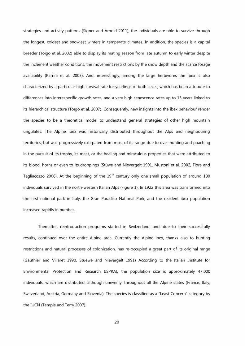
Tagliacozzo 2006). At the beginning of the 19th
century only one small population of around 100
individuals survived in the north-western Italian Alps (Figure 1). In 1922 this area was transformed into
the first national park in Italy, the Gran Paradiso National Park, and the resident ibex population
increased rapidly in number.
Thereafter, reintroduction programs started in Switzerland, and, due to their successfully
results, continued over the entire Alpine area. Currently the Alpine ibex, thanks also to hunting
restrictions and natural processes of colonization, has re-occupied a great part of its original range
(Gauthier and Villaret 1990, Stuewe and Nievergelt 1991) According to the Italian Institute for
Environmental Protection and Research (ISPRA), the population size is approximately 47.000
individuals, which are distributed, although unevenly, throughout all the Alpine states (France, Italy,
Switzerland, Austria, Germany and Slovenia). The species is classified as a “Least Concern” category by
the IUCN (Temple and Terry 2007).
21
Across the Italian Alps, the Alpine ibex has an estimated population size of about 15.600
individuals (ISPRA, 2013), but there is a problem beyond the total number of individuals. Although the
species has recovered steadily over the years to its present total populations size, its distribution is still
extremely fragmented (Dupre et al. 2001, Pedrotti et al. 2007, Carnevali et al. 2009), especially in the
eastern Alps. Here it is possible to identify almost half of the 53 total colonies described in Italy
(Carnevali et al. 2009), with small the population sizes, often lower than 100-150 individuals, and no, or
very limited, connectivity. The average densities calculated with respect to the area occupied by the
colonies vary between a minimum of 2.9 individuals/km2 in the eastern Alps to 3.2 individuals/ km
2
and 3.8 individuals/km2 in the Western and Central Alps respectively. The risks of small and isolated
populations constitute a critical issue for their conservation since environmental, demographic or
genetic stochasticity may increase the probability of extinction (Soulé 1987). An environmental
catastrophe, an animal disease, loss of genetic variation, inbreeding processes, or the combination of
such factors may interact with the growth rates of the population raising the likelihood of its collapse
(Soulé 1980; Frankel and Soulé 1981, Keller et al. 2002). Therefore, the ibex populations across the
eastern Alps may not be considered as safe. One of the main risks to the Alpine ibex is the low
population size within each colony and the scarce genetic variability (Randi et al. 1990). Recently, in the
Eastern Italian Alps the species has also experienced the effects of a parasitic infection by the scabies
mite (Sarcoptes scabiei), which has led to a steep decline in some isolated populations, such as the
colony of the Marmolada massif (Rossi et al. 2006, 2007). Also the theoretical impact of climate change
on alpine ecosystems may be suggested as a threath for the survival of the species (Grøtan et al. 2008,
Grabherr et al. 2010, Mysterud and Austrheim 2014). Therefore, from a conservation point of view, the
knowledge of how the interaction between the animal behaviour and their environment influence the
dynamics of such small and isolated ibex populations should represent one of the main purposes to
establish an effective management of the Alpine ibex.

22
4.6
4.8
5
5.2
5.4
5.6
2004 2006 2008 2010 2012 2014 2016
log
(N
)
Year
4. The study area
4.1 A separate history: results of an ongoing effort of conservation
With the translocation of 5 females and 5 males from the Gran Paradiso National Park in 1978
and 1979, a small colony of alpine ibex was established in the Marmolada-Monzoni, the highest massif
of the mountain range of the Dolomites, in the Eastern Italian Alps (Figure 1). During the two
subsequent decades, the population size of the neo-colony increased progressively up to more than
450 individuals in 2002, with an estimated growth rate (λ) of 1.24, close to the maximum rate of
increase for the species (Loison et al. 2002). However, in the snowy winter of 2003/2004, the
population was strongly reduced in number due to an epizootic of scabies mites (Monaco et al.
2005b). Less than a half of the individuals in the population survived, also due to an active project for
sanitary treatment (Rossi et al. 2006). This was followed in 2006 and 2007 by a restocking project
(Scillitani et al. 2012, 2013). Currently, the data provided by the annual counts suggest that the
population experiments a slight although progressive increase in the number of individuals (Figure 2),
with an estimated growth rate (λ) of 1.05.
Figure 2. Trend of the population of Marmolada-Monzoni after the collapse of the colony in 2004.
23
0
5
10
15
20
25
30
35
40
45
50
F M F M F
Ear tags VHF Collars GPS
Collars
Pre-collapse
Post-collapse
0
5
10
15
20
25
30
35
40
45
50
2001
2002
2003
2004
2005
2006
2007
2008
2009
2010
2011
2012
2013
2014
N
Years
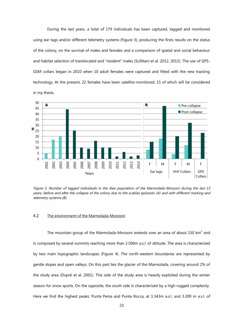
During the last years, a total of 179 individuals has been captured, tagged and monitored
using ear tags and/or different telemetry systems (Figure 3), producing the firsts results on the status
of the colony, on the survival of males and females and a comparison of spatial and social behaviour
and habitat selection of translocated and “resident” males (Scillitani et al. 2012, 2013). The use of GPS-
GSM collars began in 2010 when 10 adult females were captured and fitted with the new tracking
technology. At the present, 22 females have been satellite-monitored, 15 of which will be considered
in my thesis.
Figure 3. Number of tagged individuals in the ibex population of the Marmolada-Monzoni during the last 13
years, before and after the collapse of the colony due to the scabies epizootic (A) and with different marking and
telemetry systems (B).
4.2 The environment of the Marmolada-Monzoni
The mountain group of the Marmolada-Monzoni extends over an area of about 150 km2 and
is composed by several summits reaching more than 2.500m a.s.l. of altitude. The area is characterized
by two main topographic landscapes (Figure 4). The north-western boundaries are represented by
gentle slopes and open valleys. On this part lies the glacier of the Marmolada, covering around 2% of
the study area (Duprè et al. 2001). This side of the study area is heavily exploited during the winter
season for snow sports. On the opposite, the south side is characterized by a high rugged complexity.
Here we find the highest peaks: Punta Penia and Punta Rocca, at 3.343m a.s.l. and 3.309 m a.s.l. of
A B

24
altitude respectively. Steep rocky cliffs (Figure 6) up to 1,000 m, and narrow valleys shape the land
morphology. In this side the touristic pressure is mostly constant throughout the summer, when
activities such as hiking or climbing take place, and very scarce during winter. The temperature of the
study area may ranged in average between -20°C in winter to 18°C in summer, and the average annual
precipitation rarely exceeds the 100 mm, which means a slightly milder climate compared to other
areas in the western ibex populations (Bon et al. 2001, Parrini et al. 2003).
Figure 4. A general view of the study area. Separated by the red line: to the north-western the glacier of the
Marmolada and open valleys, to the south-eastern side the rugged complexity of the several summits and deep
valleys.
The vegetation is highly stratified following the altitudinal layers (see Scillitani et al. 2012). Up
to 1,900m a.s.l. predominates a mixed woodland composed mainly by beech (Fagus sylvatica),
common ash (Fraxinus excelsior), Norway spruce (Picea abies) and larch (Larix decidua). Above the
Glacier of the
Marmolada
25
forest line, vegetation is represented by alpine grasslands and shrubs as mountain pine (Pinus mugus)
or willows (Salix spp.). Other herbaceous species shape the last pastures before the upper slopes of
screes and rocks.
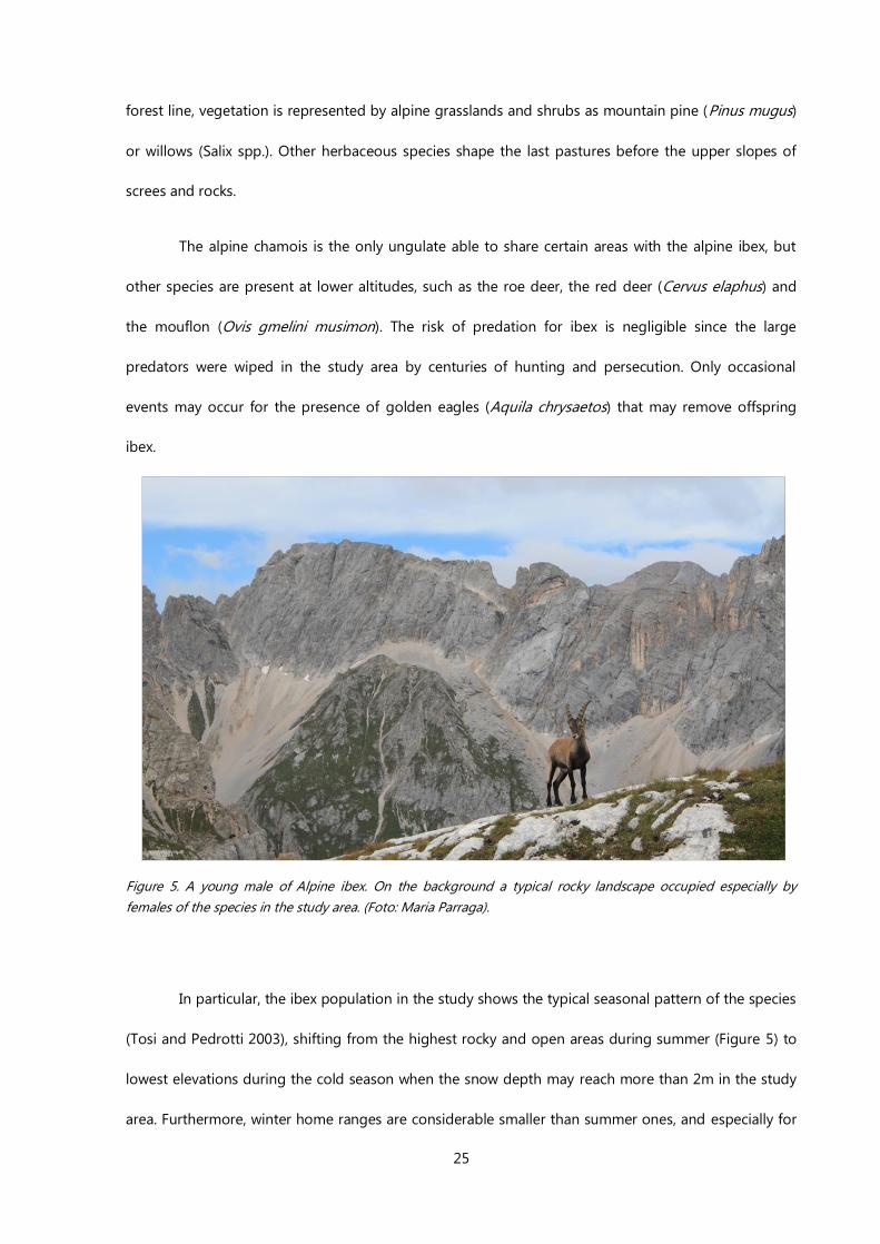
The alpine chamois is the only ungulate able to share certain areas with the alpine ibex, but
other species are present at lower altitudes, such as the roe deer, the red deer (Cervus elaphus) and
the mouflon (Ovis gmelini musimon). The risk of predation for ibex is negligible since the large
predators were wiped in the study area by centuries of hunting and persecution. Only occasional
events may occur for the presence of golden eagles (Aquila chrysaetos) that may remove offspring
ibex.
Figure 5. A young male of Alpine ibex. On the background a typical rocky landscape occupied especially by
females of the species in the study area. (Foto: Maria Parraga).
In particular, the ibex population in the study shows the typical seasonal pattern of the species
(Tosi and Pedrotti 2003), shifting from the highest rocky and open areas during summer (Figure 5) to
lowest elevations during the cold season when the snow depth may reach more than 2m in the study
area. Furthermore, winter home ranges are considerable smaller than summer ones, and especially for

26
males, they prefer to move following the altitudinal gradient within the same mountainsides rather
than travel long distances to the summer areas (Scillitani et al. 2012). The core area of seasonal home
ranges differs also between sex in location and habitat selection: while males show a strong site fidelity
occupying predominantly open grasslands over the year, females tend to use safety areas near to
rocky cliffs, probably as an antipredatory strategy (Grignolio et al. 2007), and to occupy different areas,
both on location and surface, through the seasonal periods (Scillitani et al. 2012).
5. Motivations, aims and structure of the thesis
As I suggested above, the Alpine ibex is an ideal model species to characterize the animals
adaptations to the strongly seasonality of mountain habitats, including the possible effects of a global
climate change on alpine ecosystems. It has been an important target species for sanitary studies and
studies on ecological responses of reintroduced populations, behavioural patterns of space use or
population dynamics (Villaret and Bon 1995, Mayer et al. 1997, Toïgo et al. 1999, Grignolio et al. 2004,
Scillitani et al. 2012, Mignatti et al. 2012). Most of the findings derive from the native population in the
Gran Paradiso National Park (Figure 3), or from ibex populations in the French and Swiss Alps. The
Western and Central Alps, in which these study areas are located, differ in land morphology and
vegetation composition from the Eastern Alps and the Marmolada-Monzoni groups. In addition, the
ibex colony of the Marmolada-Monzoni has had a very particular history due to the rapid population
growth, followed by the epidemic crash and the slow recovery afterwards. This fact, added to the
restricted capacity of dispersion of the species (Gauthier and Villaret 1990) and the almost complete
isolation of the population, makes it a strategic example for studying the survival strategies of the
Alpine ibex.
The powerful opportunities of new telemetry systems have led to a widespread application of
GPS devices (Douglas-Hamilton 1998, Andersen et al. 2008, Jarolímek et al. 2014), with a broad variety
27
of species and habitat types. Among wild herbivores, a great number of studies have assessed the
relationship between the animals and their habitats: roe deer (Capreolus capreolus: Rossi et al. 2003,
Cagnacci et al. 2011, Morellet et al. 2013, Saïd et al. 2009, Saïd et al. 2005, Börger et al. 2006a, 2006b);
mule deer (Odocoileus hemonus: D’Eon and Serrouya 2005, Nielson et al. 2009, Long et al. 2009,
Lendrum et al. 2014); elk (Cervus elaphus: Poole and Mowat 2005, Hebblewhite et al. 2008, Dalziel et
al. 2008, Fryxel et al. 2008, Smallidge et al. 2010, Bischof et al. 2012); moose (Alces alces: van Beest et
al. 2011, 2012). However, in particular for the Caprinae subfamily, the studies that have explored
ecological issues in mountain landscapes have focused on few species (Tibetan antelope Pantholops
hodgsonii: Leslie and Schaller 2008; Oribi Ourebia ourebi: Arcese et al. 1995; Bighorn sheep Ovis
Canadensis: Martin et al. 2013; Blue sheep Pseudois nayaur: Oli 1996; Barbary sheep Ammotragus
lervia: Cassinello and Alados 1996; Mountain goat Oreamnos americanus: Côté and Festa-Bianchet
2001; Iberian wild goat Capra pyrenaica: Perez et al. 2002; Alpine ibex Capra ibex: Marreros et al. 2012).
In all the studies reviewed on Alpine ibex, the analysed data came from direct observations of tagged
individuals, population counts, telemetric systems for metabolic measurements, or triangulation
techniques using VHF collars. I did not find studies using high frequency data from individuals
monitored with GPS collars, and I consider that it is strongly necessary to apply this powerful method
to improve the knowledge of this peculiar species. Highlighting the spatial behaviour of this ibex
population with more accurate data and at different spatial and temporal scales may also provide
essential information for the management and conservation of other colonies across the eastern Alps.
Thereby, the aims of this thesis were as follows.
Chapter I. Due to the high topographic complexity of the study area, I investigated on the factors that
might determine the performance of GPS-GSM collars, in terms of fix acquisition rates and accuracy.
Many studies have already examined such factors under various environmental features, reaching a
general agreement on the importance of canopy cover, sky view and individual activity as the main

28
variables to be taken into account before drawing results from GPS data (Biggs et al. 2001, Wells et al.
2011, Webb et al. 2013). However, I found that no studies have so far addressed the effects of such
factors on Alpine ibex in its extreme landscapes. Hence, I decided to analyze how differences in the
percentage of visible sky, the season, the habitat types, the weather and the species activity patterns
may affect the probability of receiving a location and the quality of the received data. I used both tests
with fixed collars and data collected on free-ranging ibexes, in order to understand how inherent
limitations in the methodology may induce biased conclusions. These insights are both necessary for
addressing the subsequent analyses of spatial behaviour and, in general, useful for other similar
studies in mountain habitats.
Chapter II. Having evaluated the methodological limitations associated with the use of GPS
technologies in high mountain areas, I then investigated into the general strategies of space use of
female Alpine ibex, by analyzing home range patterns at weekly and monthly scales. My aim was to
understand how extrinsic and intrinsic factors might determine patterns of individual space use. To do
this, I considered also two different spatial scales, examining both the home ranges and the core areas.
I focused the analysis first on intra-annual temporal patterns, and then, after having defined
biologically meaningful seasons, I looked within season for the effects of variables indexeing climate
and weather, food and shelter resources, and individual status. This chapter provides the most detailed
approach into the home range patterns of the species so far available to my knowledge.
Chapter III. To complement the results of chapter III, and in view of the intrinsic difficulties in sampling
and assessing vegetation and food resources in high mountain habitats, I aimed here to develop a
rapid method for estimating variations in diet quality, and tested its ability to evaluate biological
trends. I collected fresh faecal samples from observed groups of animals across the overall population
range, and then examined them for N and NDF contents using reference chemical methods and
different Near-Infrared Spectroscopy (NIR) instruments. I compared prediction accuracies and tested

29
how different methods were able to identify temporal patterns of diet quality from summer through
autumn, and differences between males and females. Moreover, I explored the relationship between
the vegetation phenology, expressed as NDVI, and the seasonal trends in N and NDF faecal content.
The results of this chapter provide additional knowledge on the applicability of a rapid, non-invasive
technique for indexing diet quality, and on how the species might respond to seasonal variations in
foode resources and energetic requirements.
30
LITERATURE CITED
Adrados, C., Girard, I., Gendner, J. P., and Janeau, G. (2002). Global positioning system (GPS) location
accuracy improvement due to selective availability removal. Comptes Rendus Biologies, 325(2), 165-
170.
Amstrup, S. C., and Durner, G. M. (1995). Survival rates of radio-collared female polar bears and their
dependent young. Canadian Journal of Zoology, 73(7), 1312-1322.
Andersen, M., Derocher, A. E., Wiig, Ø., and Aars, J. (2008). Movements of two Svalbard polar bears
recorded using geographical positioning system satellite transmitters. Polar Biology, 31(8), 905-911.
Arcese, P., Jongejan, G., and Sinclair, A. R. E. (1995). Behavioural flexibility in a small African antelope:
group size and composition in the oribi (Ourebia ourebi, Bovidae). Ethology, 99(1‐2), 1-23.
Aublet, J. F., Festa-Bianchet, M., Bergero, D., and Bassano, B. (2009). Temperature constraints on
foraging behaviour of male Alpine ibex (Capra ibex) in summer. Oecologia, 159(1), 237-247.
Bartos, L., Vankova, D., Miller, K. V., and Siler, J. (2002). Interspecific competition between white-tailed,
fallow, red, and roe deer. The Journal of wildlife management, 522-527.
Biggs, J. R., Bennett, K. D., and Fresquez, P. R. (2001). Relationship between home range characteristics
and the probability of obtaining successful global positioning system (GPS) collar positions for elk in
New Mexico. Western North American Naturalist, 61(2), 213-222.
Bischof, R., Loe, L. E., Meisingset, E. L., Zimmermann, B., Van Moorter, B., and Mysterud, A. (2012). A
migratory northern ungulate in the pursuit of spring: Jumping or surfing the green wave?. The
American Naturalist, 180(4), 407-424.
Bon, R., Rideau, C., Villaret, J. C., and Joachim, J. (2001). Segregation is not only a matter of sex in
Alpine ibex (Capra ibex ibex) Animal Behaviour, 62(3), 495-504.
Börger, L., Franconi, N., De Michele, G., Gantz, A., Meschi, F., Manica, A., ... and Coulson, T. I. M. (2006a).
Effects of sampling regime on the mean and variance of home range size estimates. Journal of Animal
Ecology, 75(6), 1393-1405.
Börger, L., Franconi, N., Ferretti, F., Meschi, F., De Michele, G., Gantz, A., and Coulson, T. (2006b). An
integrated approach to identify spatiotemporal and individual‐level determinants of animal home
range size. The American Naturalist, 168(4), 471-485.
Boschi, C., and Nievergelt, B. (2003). The spatial patterns of Alpine chamois (Rupicapra rupicapra
rupicapra) and their influence on population dynamics in the Swiss National Park. Mammalian Biology-
Zeitschrift für Säugetierkunde, 68(1), 16-30.
Bowman, J. L., Kochanny, C. O., Demarais, S., and Leopold, B. D. (2000). Evaluation of a GPS collar for
white-tailed deer. Wildlife Society Bulletin, 141-145.
Bradshaw, C. J., Boutin, S., and Hebert, D. M. (1997). Effects of petroleum exploration on woodland
caribou in northeastern Alberta. The Journal of wildlife management, 1127-1133.
Bradshaw, W. E., and Holzapfel, C. M. (2007). Evolution of animal photoperiodism. Annual Review of
Ecology, Evolution, and Systematics, 1-25.

31
Bremset Hansen, B., Herfindal, I., Aanes, R., Sæther, B. E., and Henriksen, S. (2009). Functional response
in habitat selection and the tradeoffs between foraging niche components in a large herbivore. Oikos,
118(6), 859-872.
Cagnacci, F., Boitani, L., Powell, R. A., and Boyce, M. S. (2010). Animal ecology meets GPS-based
radiotelemetry: a perfect storm of opportunities and challenges. Philosophical Transactions of the
Royal Society B: Biological Sciences, 365(1550), 2157-2162.
Cagnacci, F., Focardi, S., Heurich, M., Stache, A., Hewison, A. J., Morellet, N., Kjellander, P., Linnell, J.D.C,
Mysterud, A., Neteler, M., Delucchi, L., Ossi, F. and Urbano, F. (2011). Partial migration in roe deer:
migratory and resident tactics are end points of a behavioural gradient determined by ecological
factors. Oikos, 120(12), 1790-1802.
Cargnelutti, B., Coulon, A., Hewison, A. J., Goulard, M., ANGIBAULT, J., and Morellet, N. (2007). Testing
Global Positioning System performance for wildlife monitoring using mobile collars and known
reference points. The Journal of wildlife management, 71(4), 1380-1387.
Carnevali L, Pedrotti L, Riga F and Toso S (2009). Ungulates in Italy: Status, distribution, abundance,
management and hunting of Ungulate populations in Italy - Report 2001-2005. Biol Cons Fauna, 117,
Istituto Nazionale Fauna Selvatica.
Cassinello, J., and Alados, C. L. (1996). Female reproductive success in captive Ammotragus lervia
(Bovidae, Artiodactyla). Study of its components and effects of hierarchy and inbreeding. Journal of
Zoology, 239(1), 141-153.
Colchero, F., Medellin, R. A., Clark, J. S., Lee, R., and Katul, G. G. (2009). Predicting population survival
under future climate change: density dependence, drought and extraction in an insular bighorn sheep.
Journal of animal ecology, 78(3), 666-673.
Côté, S. D., and Festa-Bianchet, M. (2001). Reproductive success in female mountain goats: the
influence of age and social rank. Animal Behaviour, 62(1), 173-181.
Coulombe, M. L., Massé, A., and Côté, S. D. (2006). Quantification and accuracy of activity data
measured with VHF and GPS telemetry. Wildlife Society Bulletin, 34(1), 81-92.
Dalziel, B. D., Morales, J. M., & Fryxell, J. M. (2008). Fitting probability distributions to animal movement
trajectories: using artificial neural networks to link distance, resources, and memory. The American
Naturalist, 172(2), 248-258.
D'Eon, R. G., Serrouya, R., Smith, G., and Kochanny, C. O. (2002). GPS radiotelemetry error and bias in
mountainous terrain. Wildlife Society Bulletin, 430-439.
D'Eon, R. G., and Serrouya, R. (2005). Mule deer seasonal movements and multiscale resource selection
using global positioning system radiotelemetry. Journal of Mammalogy, 86(4), 736-744.
Douglas-Hamilton, I. (1998). Tracking African elephants with a global positioning system (GPS) radio
collar. Pachyderm, (25), 81-92.
Duprè E., Pedrotti L. and Arduino S. (2001) Alpine ibex conservation strategy. The Alpine ibex in the
Italian Alps: status, potential distribution and management options for conservation and sustainable
development. Available online at: http://biocenosi.dipbsf.uninsubria.it/LHI/
Dussault, C., Courtois, R., Ouellet, J. P., and Huot, J. (1999). Evaluation of GPS telemetry collar
performance for habitat studies in the boreal forest. Wildlife Society Bulletin, 965-972.
32
Dussault, C., Courtois, R., Ouellet, J. P., and Huot, J. (2001). Influence of satellite geometry and
differential correction on GPS location accuracy. Wildlife Society Bulletin, 171-179.
Dussault, C., Courtois, R., Ouellet, J. P., and Girard, I. (2005). Space use of moose in relation to food
availability. Canadian journal of zoology, 83(11), 1431-1437.
Fancy, S. G., and Whitten, K. R. (1991). Selection of calving sites by Porcupine herd caribou. Canadian
Journal of Zoology, 69(7), 1736-1743.
Ferguson, S. H. (2002). The effects of productivity and seasonality on life history: comparing age at
maturity among moose (Alces alces) populations. Global Ecology and Biogeography, 11(4), 303-312.
Festa-Bianchet, M., and Côté, S. D. (2007). Mountain goats: ecology, behavior, and conservation of an
alpine ungulate. Island Press.
Fieberg, J., Matthiopoulos, J., Hebblewhite, M., Boyce, M. S., & Frair, J. L. (2010). Correlation and studies
of habitat selection: problem, red herring or opportunity?. Philosophical Transactions of the Royal
Society of London B: Biological Sciences, 365(1550), 2233-2244.
Fiore, I., and Tagliacozzo, A. (2006). Lo sfruttamento dello stambecco nel Tardiglaciale di Riparo
Dalmeri (TN): il livello 26c.
Frair, J. L., Nielsen, S. E., Merrill, E. H., Lele, S. R., Boyce, M. S., Munro, R. H., ... and Beyer, H. L. (2004).
Removing GPS collar bias in habitat selection studies. Journal of Applied Ecology, 41(2), 201-212.
Frair, J. L., Fieberg, J., Hebblewhite, M., Cagnacci, F., DeCesare, N. J., and Pedrotti, L. (2010). Resolving
issues of imprecise and habitat-biased locations in ecological analyses using GPS telemetry data.
Philosophical Transactions of the Royal Society B: Biological Sciences, 365(1550), 2187-2200.
Frankel OH, Soulé ME (1981) Conservation and Evolution. Cambridge University Press.
Fryxell, J. M., Hazell, M., Börger, L., Dalziel, B. D., Haydon, D. T., Morales, J. M., ... and Rosatte, R. C.
(2008). Multiple movement modes by large herbivores at multiple spatiotemporal scales. Proceedings
of the National Academy of Sciences, 105(49), 19114-19119.
Gaillard, J. M., Hebblewhite, M., Loison, A., Fuller, M., Powell, R., Basille, M., & Van Moorter, B. (2010).
Habitat–performance relationships: finding the right metric at a given spatial scale. Philosophical
Transactions of the Royal Society B: Biological Sciences, 365(1550), 2255-2265.
Gauthier, D., and Villaret, J. C. (1990). La réintroduction en France du bouquetin des Alpes. Revue
d’Ecologie (la Terre et la Vie) Supplement, 5, 97-120.
Giuggioli, L., and Bartumeus, F. (2010). Animal movement, search strategies and behavioural ecology: a
cross‐disciplinary way forward. Journal of animal ecology, 79(4), 906-909.
Grabherr, G., Gottfried, M., and Pauli, H. (2010). Climate change impacts in alpine environments.
Geography Compass, 4(8), 1133-1153.
Graves, T. A., and Waller, J. S. (2006). Understanding the causes of missed global positioning system
telemetry fixes. Journal of Wildlife Management, 70(3), 844-851.
Grignolio, S., Rossi, I., Bassano, B., Parrini, F., and Apollonio, M. (2004). Seasonal variations of spatial
behaviour in female Alpine ibex (Capra ibex ibex) in relation to climatic conditions and age. Ethology
Ecology and Evolution, 16(3), 255-264.

33
Grignolio, S., Rossi, I., Bassano, B., and Apollonio, M. (2007). Predation risk as a factor affecting sexual
segregation in Alpine ibex. Journal of Mammalogy, 88(6), 1488-1497.
Grøtan, V., SÆther, B. E., Filli, F., and Engen, S. (2008). Effects of climate on population fluctuations of
ibex. Global Change Biology, 14(2), 218-228.
Hamel, S., and Côté, S. D. (2007). Habitat use patterns in relation to escape terrain: are alpine ungulate
females trading off better foraging sites for safety?. Canadian Journal of Zoology, 85(9), 933-943.
Hamel, S., Garel, M., Festa‐Bianchet, M., Gaillard, J. M., and Côté, S. D. (2009). Spring Normalized
Difference Vegetation Index (NDVI) predicts annual variation in timing of peak faecal crude protein in
mountain ungulates. Journal of Applied Ecology, 46(3), 582-589.
Hamr, J. (1988). Disturbance behaviour of chamois in an alpine tourist area of Austria. Mountain
Research and Development, 65-73.
Heard, D. C., Ciarniello, L. M., and Seip, D. R. (2008). Grizzly bear behavior and global positioning
system collar fix rates. The Journal of Wildlife Management, 72(3), 596-602.
Hebblewhite, M., Merrill, E., and McDermid, G. (2008). A multi-scale test of the forage maturation
hypothesis in a partially migratory ungulate population. Ecological monographs, 78(2), 141-166.
Hebblewhite, M., and Haydon, D. T. (2010). Distinguishing technology from biology: a critical review of
the use of GPS telemetry data in ecology. Philosophical Transactions of the Royal Society B: Biological
Sciences, 365(1550), 2303-2312.
Herrero, J., Garin, I., García-Serrano, A., and García-González, R. (1996). Habitat use in a Rupicapra
pyrenaica pyrenaica forest population. Forest Ecology and Management, 88(1), 25-29.
Hilderbrand, G. V., Hanley, T. A., Robbins, C. T., and Schwartz, C. C. (1999). Role of brown bears (Ursus
arctos) in the flow of marine nitrogen into a terrestrial ecosystem. Oecologia, 121(4), 546-550.
Horne, J. S., Garton, E. O., Krone, S. M., and Lewis, J. S. (2007). Analyzing animal movements using
Brownian bridges. Ecology, 88(9), 2354-2363.
Jacobson, A. R., Provenzale, A., von Hardenberg, A., Bassano, B., and Festa-Bianchet, M. (2004). Climate
forcing and density dependence in a mountain ungulate population. Ecology, 85(6), 1598-1610.
arol mek, ., Van k, ., e ek, M., Masner, J., and Stoces, M. (2014). The telemetric tracking of wild boar
as a tool for field crops damage limitation. Plant, Soil and Environment, 60(9), 418-425.
Johnson, A. R., Wiens, J. A., Milne, B. T., and Crist, T. O. (1992). Animal movements and population
dynamics in heterogeneous landscapes. Landscape ecology, 7(1), 63-75.
Keller, L. F., and Waller, D. M. (2002). Inbreeding effects in wild populations. Trends in Ecology
Lamberti, P., Rossi, I., Mauri, L., and Apollonio, M. (2001). Alternative use of space strategies of female
roe deer (Capreolus capreolus) in a mountainous habitat. Italian Journal of Zoology, 68(1), 69-
73.Lamberti,
Lamberti, P., Mauri, L., Merli, E., Dusi, S., & Apollonio, M. (2006). Use of space and habitat selection by
roe deer Capreolus capreolus in a Mediterranean coastal area: how does woods landscape affect home
range?. Journal of Ethology, 24(2), 181-188.
34
Lawlor, D. W. (1995). Photosynthesis, productivity and environment. Journal of Experimental Botany,
46(special issue), 1449-1461.
Lendrum, P. E., Anderson Jr, C. R., Monteith, K. L., Jenks, J. A., and Bowyer, R. T. (2014). Relating the
movement of a rapidly migrating ungulate to spatiotemporal patterns of forage quality. Mammalian
Biology-Zeitschrift für Säugetierkunde.
Leslie Jr, D. M., and Schaller, G. B. (2008). Pantholops hodgsonii (Artiodactyla: Bovidae). Mammalian
Species, 1-13.
Loison A., Toigo C., Appolinaire J. and Michallet J. (2002). Demographic processes in colonizing
populations of isard (Rupicapra pyrenaica) and ibex (Capra ibex). J. Zool., London 256: 199-205.
Long, R. A., Kie, J. G., Terry Bowyer, R., and Hurley, M. A. (2009). Resource selection and movements by
female mule deer Odocoileus hemionus: effects of reproductive stage. Wildlife Biology, 15(3), 288-298
Månsson, J., Andrén, H., Pehrson, Å., and Bergström, R. (2007). Moose browsing and forage availability:
a scale-dependent relationship?. Canadian Journal of Zoology, 85(3), 372-380.
Marreros, N., Frey, C. F., Willisch, C. S., Signer, C., and Ryser-Degiorgis, M. P. (2012). Coprological
analyses on apparently healthy Alpine ibex (Capra ibex ibex) from two Swiss colonies. Veterinary
parasitology, 186(3), 382-389.
Martin, A. M., Presseault-Gauvin, H., Festa-Bianchet, M., and Pelletier, F. (2013). Male mating
competitiveness and age-dependent relationship between testosterone and social rank in bighorn
sheep. Behavioral Ecology and Sociobiology, 67(6), 919-928.
Mason, T. H., Stephens, P. A., Apollonio, M., and Willis, S. G. (2014). Predicting potential responses to
future climate in an alpine ungulate: interspecific interactions exceed climate effects. Global change
biology, 20(12), 3872-3882.
Mayer, D., Degiorgis, M. P., Meier, W., Nicolet, J., and Giacometti, M. (1997). Lesions associated with
infectious keratoconjunctivitis in alpine ibex. Journal of wildlife diseases, 33(3), 413-419.
Mcloughlin, P. D., Ferguson, S. H., and Messier, F. (2000). Intraspecific variation in home range overlap
with habitat quality: a comparison among brown bear populations. Evolutionary Ecology, 14(1), 39-60.
Mech, L. D. 1967. Telemetry as a technique in the study of predation. J. Wildl. Manage. 31:492-496.
Mech, L. D., and Barber, S. M. (2002). A critique of wildlife radio-tracking and its use in national parks. A
report to the US National Park Service, 19-20.
Merrill, S. B., Adams, L. G., Nelson, M. E., and Mech, L. D. (1998). Testing releasable GPS radiocollars on
wolves and white-tailed deer. Wildlife Society Bulletin, 830-835.
Merrill, S. B., and Mech, L.D. (2000). Details of extensive movements by Minnesota wolves (Canis lupus).
The American Midland Naturalist, 144(2), 428-433.
Mignatti, A., Casagrandi, R., Provenzale, A., von Hardenberg, A., and Gatto, M. (2012). Sex-and age-
structured models for Alpine ibex Capra ibex ibex population dynamics. Wildlife Biology, 18(3), 318-
332.
Minder, I. (2012). Local and seasonal variations of roe deer diet in relation to food resource availability
in a Mediterranean environment. European Journal of Wildlife Research, 58(1), 215-225.

35
Moen, R., Pastor, J., and Cohen, Y. (1996). Interpreting behavior from activity counters in GPS collars on
moose. Alces, 1996(32), 101-108.
Moen, R., Pastor, J., and Cohen, Y. (1997). Accuracy of GPS telemetry collar locations with differential
correction. The Journal of wildlife management, 530-539.
Monaco A., Nicoli F., Gilio N.and Fraquelli C. (2005b). Effetti demografici della mortalita invernale e
della rogna sarcoptica nella popolazione di stambecco della Marmolada. Pag 104. In: Prigioni et
al.(eds) V Congr. It. Teriologia, Hystrix, It. J. Mamm.,(N.S.) SUPP.
Morales, J. M., Moorcroft, P. R., Matthiopoulos, J., Frair, J. L., Kie, J. G., Powell, R. A., ... & Haydon, D. T.
(2010). Building the bridge between animal movement and population dynamics. Philosophical
Transactions of the Royal Society B: Biological Sciences, 365(1550), 2289-2301.
Morellet, N., Bonenfant, C., Börger, L., Ossi, F., Cagnacci, F., Heurich, M., ... and Mysterud, A. (2013).
Seasonality, weather and climate affect home range size in roe deer across a wide latitudinal gradient
within Europe. Journal of Animal Ecology, 82(6), 1326-1339.
Morrison, S. F., Pelchat, G., Donahue, A., and Hik, D. S. (2009). Influence of food hoarding behavior on
the over-winter survival of pikas in strongly seasonal environments. Oecologia, 159(1), 107-116.
Mustoni, A. (2002). Ungulati delle Alpi. Nitida immagine.
Mysterud, A. (1999). Seasonal migration pattern and home range of roe deer (Capreolus capreolus) in
an altitudinal gradient in southern Norway. Journal of Zoology, 247(4), 479-486.
Mysterud, A., and Austrheim, G. (2014). Lasting effects of snow accumulation on summer performance
of large herbivores in alpine ecosystems may not last. Journal of Animal Ecology, 83(3), 712-
719Nathan, R., Getz, W.
Nathan, R. (2008). An emerging movement ecology paradigm. Proceedings of the National Academy
of Sciences, 105(49), 19050-19051.
Nielson, R. M., Manly, B. F., McDonald, L. L., Sawyer, H., and McDonald, T. L. (2009). Estimating habitat
selection when GPS fix success is less than 100%. Ecology, 90(10), 2956-2962.
Oli, M. K. (1996). Seasonal patterns in habitat use of blue sheep Pseudois nayaur (Artiodactyla,
Bovidae) in Nepal. Mammalia, 60(2), 187-194.
Parrini, F., Grignolio, S., Luccarini, S., Bassano, B., and Apollonio, M. (2003). Spatial behaviour of adult
male Alpine ibex Capra ibex ibex in the Gran Paradiso National Park, Italy. Acta Theriologica, 48(3),
411-423.
Pedrotti L., Carnevali L., Monaco A., Bassano B., Tosi G., Riga F. and Toso S. (2007) Alpine ibex or the
duty of re-introduction. Recovery history, status, and future management in the Italian alps. Abstract
in: Prigioni C. and Sforzi A. (eds.). Abstracts V European Congress of Mammalogy, Hystrix It J Mamm,
(N S) Vol. I-2, Supp (2007): 1-586
Pérez, J. M., Granados, J. E., Soriguer, R. C., Fandos, P., Márquez, F. J., and Crampe, J. P. (2002).
Distribution, status and conservation problems of the Spanish Ibex, Capra pyrenaica (Mammalia:
Artiodactyla)†. Mammal Review, 32(1), 26-39.
Poole, K. G., and Mowat, G. (2005). Winter habitat relationships of deer and elk in the temperate
interior mountains of British Columbia. Wildlife Society Bulletin, 33(4), 1288-1302.

36
Ramanzin, M., Sturaro, E., and Zanon, D. (2007). Seasonal migration and home range of roe deer
(Capreolus capreolus) in the Italian eastern Alps. Canadian journal of zoology, 85(2), 280-289.
Randi, E., Tosi, G., Toso, S., Lorenzini, R., & Fusco, G. (1990). Genetic variability and conservation
problems in Alpine ibex and feral goat populations (genus Capra). Zeitschrift für Säugetierkunde, 55(6),
413-420.
Rempel, R. S., Rodgers, A. R., and Abraham, K. F. (1995). Performance of a GPS animal location system
under boreal forest canopy. The Journal of wildlife management, 543-551.
Rivrud, I. M., Loe, L. E., and Mysterud, A. (2010). How does local weather predict red deer home range
size at different temporal scales?. Journal of Animal Ecology, 79(6), 1280-1295.
Rodgers, A. R., and Anson, P. (1994). Animal-borne GPS: Tracking the habitat. GPS World, 5(7), 20-33.
Rodgers, A. R., Rempel, R. S., and Abraham, K. F. (1996). A GPS-based telemetry system. Wildlife Society
Bulletin, 559-566.
Rossi, I., Lamberti, P., Mauri, L., and Apollonio, M. (2003). Home range dynamics of male roe deer
Capreolus capreolus in a mountainous habitat. Acta theriologica, 48(3), 425-432.
Rossi, L., Menzano, A., Sommavilla, G. M., De Martin, P., Cadamuro, A., Rodolfi, M., and Coleselli, A. and
Ramanzin M (2006). Actions for the recovery o fan Alpine ibex herd affected by epidemic scabies: the
Marmolada case, Italy. In Abstract of the 3rd International Conference on Alpine ibex (pp. 12-14).
Rossi, L., Fraquelli, C., Vesco, U., Permunian, R., Sommavilla, G. M., Carmignola, G., ... and Meneguz, P. G.
(2007). Descriptive epidemiology of a scabies epidemic in chamois in the Dolomite Alps, Italy.
European Journal of Wildlife Research, 53(2), 131-141.
Rumble, M. A., Benkobi, L., Lindzey, F., and Gamo, R. S. (2001). Evaluating elk habitat interactions with
GPS collars. Tracking animals with GPS, 11.
Saïd, S., Gaillard, J. M., Duncan, P., Guillon, N., Guillon, N., Servanty, S., ... and Laere, G. (2005). Ecological
correlates of home‐range size in spring–summer for female roe deer (Capreolus capreolus) in a
deciduous woodland. Journal of Zoology, 267(3), 301-308.
Said, S., Gaillard, J. M., Widmer, O., Débias, F., Bourgoin, G., Delorme, D., and Roux, C. (2009). What
shapes intra‐specific variation in home range size? A case study of female roe deer. Oikos, 118(9),
1299-1306.
Scillitani, L., Sturaro, E., Menzano, A., Rossi, L., Viale, C., and Ramanzin, M. (2012). Post-release spatial
and social behaviour of translocated male Alpine ibexes (Capra ibex ibex) in the eastern Italian Alps.
European Journal of Wildlife Research, 58(2), 461-472
Scillitani, L., Darmon, G., Monaco, A., Cocca, G., Sturaro, E., Rossi, L., and Ramanzin, M. (2013). Habitat
selection in translocated gregarious ungulate species: an interplay between sociality and ecological
requirements. The Journal of Wildlife Management, 77(4), 761-769.
Signer, C., Ruf, T., and Arnold, W. (2011). Hypometabolism and basking: the strategies of Alpine ibex to
endure harsh over‐wintering conditions. Functional Ecology, 25(3), 537-547.
Simmons, W. W. (1968). An introduction to biotelemetry. Journal of Occupational and Environmental
Medicine, 10(4), 188-194.

37
Singh, N. J., and Ericsson, G. (2014). Changing motivations during migration: linking movement speed
to reproductive status in a migratory large mammal. Biology letters, 10(6), 20140379.
Smallidge, S. T., Baker, T. T., VanLeeuwen, D., Gould, W. R., and Thompson, B. C. (2010). Elk distributions
relative to spring normalized difference vegetation index values. International Journal of Ecology, 2010.
Solounias, N. I. K. O. S. (2007). Family bovidae. The evolution of artiodactyls, 278-291.
Soulé ME (1980) Thresholds for survival: maintaining fitness and evolutionary potential. In:
Conservation Biology: An Evolutionary-Ecological Perspective (eds. Soulé ME, Wilcox B), pp. 151-170.
Sinauer Associates, Sunderland.
Soulé ME (1987) Viable populations for conservations. Cambridge University Press, Cambridge.
Stüwe, M., and Nievergelt, B. (1991). Recovery of alpine ibex from near extinction: the result of effective
protection, captive breeding, and reintroductions. Applied Animal Behaviour Science, 29(1), 379-387.
Tchamba, M. N., Bauer, H., and Iongh, H. D. (1995). Application of VHF‐radio and satellite telemetry
techniques on elephants in northern Cameroon. African Journal of Ecology, 33(4), 335-346.
Telfer, E. S., and Kelsall, J. P. (1984). Adaptation of some large North American mammals for survival in
snow. Ecology, 1828-1834.
Temple H. J. and Terry A. (Compilers) (2007) The Status and Distribution of European Mammals.
Luxembourg: Office for Official Publications of the European Communities
Toïgo, C., Gaillard, J. M., and Michallet, J. (1999). Cohort affects growth of males but not females in
alpine ibex (Capra ibex ibex). Journal of Mammalogy, 1021-1027.
Toïgo, C., Gaillard, J. M., Gauthier, D., Girard, I., Martinot, J.P., and Michallet, J. (2002). Female
reproductive success and costs in an alpine capital breeder under contrasting environments.
Ecoscience, 427-433.
Toïgo, C., Gaillard, J. M., Fersta-Bianchet, M., Largo, E., Michallet, J., and Maillard, D. (2007). Sex-
andage- specific survival of the highly dimorphic Alpine ibex: evidence for a conservative life-history
tactic. Journal of Animal Ecology, 76(4), 679-686.
Tomkiewicz, S. M., Fuller, M. R., Kie, J. G., and Bates, K. K. (2010). Global positioning system and
associated technologies in animal behaviour and ecological research. Philosophical Transactions of the
Royal Society B: Biological Sciences, 365(1550), 2163-2176.
Tosi, G., and Pedrotti, L. (2003). Capra ibex L. Fauna d’Italia. Mammalia III Carnivora-Artiodactyla.
Calderini Edagricole, Bologna, 364-434.
Turunen, M., Soppela, P., Kinnunen, H., Sutinen, M. L., and Martz, F. (2009). Does climate change
influence the availability and quality of reindeer forage plants?. Polar Biology, 32(6), 813-832.
van Beest, F. M., Rivrud, I. M., Loe, L. E., Milner, J. M., and Mysterud, A. (2011). What determines
variation in home range size across spatiotemporal scales in a large browsing herbivore?. Journal of
Animal Ecology, 80(4), 771-785.
van Beest, F. M., Van Moorter, B., and Milner, J. M. (2012). Temperature-mediated habitat use and
selection by a heat-sensitive northern ungulate. Animal Behaviour, 84(3), 723-735.
38
Villaret, J. C., & Bon, R. (1995). Social and spatial segregation in Alpine ibex (Capra ibex) in Bargy,
French Alps. Ethology, 101(4), 291-300.
Vuren, D. V., and Armitage, K. B. (1991). Duration of snow cover and its influence on life-history
variation in yellow-bellied marmots. Canadian Journal of Zoology, 69(7), 1755-1758.
Webb, S. L., Dzialak, M. R., Mudd, J. P., & Winstead, J. B. (2013). Developing spatially-explicit weighting
factors to account for bias associated with missed GPS fixes in resource selection studies. Wildlife
Biology, 19(3), 257-273.
Wells, A. G., Wallin, D. O., Rice, C. G., and Chang, W. Y. (2011). GPS bias correction and habitat selection
by mountain goats. Remote Sensing, 3(3), 435-459.
Wiegand, T., Naves, J., Garbulsky, M. F., and Fernández, N. (2008). Animal habitat quality and
ecosystem functioning: exploring seasonal patterns using NDVI. Ecological Monographs, 78(1), 87-103

39
CHAPTER 1
LAND MORPHOLOGY, SEASON AND INDIVIDUAL
ACTIVITY INFLUENCE GPS FIX ACQUISITION RATES AND
LOCATION ERROR IN AN ALPINE UNGULATE
PARRAGA M.A., STURARO E., RAMANZIN M.


41
INTRODUCTION
During the last decades, the technologies applied to wildlife studies have experienced most
significant advances. Following the use of conventional very high-frequency (VHF) triangulation
techniques, the new Global Position System (GPS) radiotelemetry has greatly increased the possibility
to analyze use of habitats, behavior and activity patterns for free-ranging animals over a broad range
of temporal and spatial scales (Fuller et al. 2005, Cooke et al. 2004, Handcock et al. 2009).
However, limitations of GPS technologies remain under study because of two main types of
error. The first is the variable ability of GPS transmitters to acquire an animal location (Fix Acquisition
Rate, FAR). Missing data do not occur randomly, but depend on several factors such us topography
(D’Eon et al. 2002), canopy cover (Moen et al. 1996, Rumble and Lindzey 1997, Heard et al. 2008),
vegetation characteristics (Janeau et al. 2004, Hansen and Riggs 2008), or animal activity (Graves and
Waller 2006, Cargnelutti et al. 2007). Missed locations can influence the estimates of resources used by
animals, generating biased conclusions for habitats where fix success is limited. This bias effect
depends on the proportion of data lost, the frequency of use of biased habitat types by individuals,
and the spatial association among habitat types (Rettie and McLoughlin 1999). The second source of
error is the location inaccuracy (Location Error, LE), which is the difference between the estimated
position and the true position. A GPS device must simultaneously receive signals from at least 3
satellites to calculate a location, and the total number of satellites used determines whether a two-
dimensional (at least 3 satellites) or a three-dimensional (more than 3 satellites) position is obtained.
These two categories are conventionally identified with the 2D or 3D navigation (NAV) classification.
The number of visible satellites, and therefore positional accuracy, can be affected by physical
obstructions between the GPS device and available satellites orbiting the earth. Several studies
(Adrados et al. 2002, Lewis et al. 2007, Sager-Fradkin et al. 2007) have addressed location accuracy
focusing on fix quality (2D or 3D and an associated index of satellite geometry based on a dilution of

42
precision (DOP)). These studies outlined the effects of rugged topography and vegetation cover
(Dussault et al. 1999, Gamo et al. 2000, D’Eon et al. 2002, DeCesare et al. 2005), as well as that of collar
orientation (Girard et al. 2002, D’Eon and Delparte 2005, Jiang et al. 2008) on location accuracy.
However, unequivocal quantitative methods of screening GPS radio-telemetry data are currently
unavailable, and failing to account for location inaccuracy can lead to a misclassification of resource
selection and to an incorrect interpretation of results (Nielson et al. 2009).
Fix acquisition rates and GPS accuracy are frequently studied using stationary tests with fixed
collars positioned in different habitat types, for a given periods of time, and with pre-determined
temporal intervals. These tests are useful to model FAR and location Error (LE) under different
environmental conditions, can be replicated across a range of spatial and temporal variation, and are
readily comparable among study sites and time periods (Cagnacci et al. 2010). However, GPS errors are
also related to unknown factors that may be linked to the interaction between the behaviour of free-
ranging animals and the features of the habitats that they use (D’Eon 2003). For instance, comparisons
of the results from fixed GPS collars at known locations with the results from collars fitted to free-
ranging animals suggest that fixed collars overestimate FAR (Zweifel-Schielly and Suter 2007, Denis et
al 2010, Guthrie et al. 2011, Wells et al. 2011), especially at short fix intervals (Cain et al. 2005). In fact,
GPS collars performance depends also on types of behavior, such as walking or standing, or lying, and
on meteorological conditions, which are expected to be related to habitat selection (Edenius 1996,
Heard et al. 2008, Bourgoin et al. 2009, Webb et al. 2013).
Most of the studies aiming to identify sources of bias and inaccuracy of GPS tracking devices
have been conducted on gentle mountain or forested landscapes, where missing data or location
errors occur mainly due to canopy closure or collar orientation (Gamo and Rumble 2000, Janeau et al.
2004, Jiang et al. 2008, Williams et al. 2012). More work is needed to understand and quantify the
factors affecting GPS performance in high mountain landscapes, where topographic complexity and
terrain ruggedness can lead to lower FAR, higher proportions of 2D fixes, and higher LE than in

43
lowlands (Zweifel-Schielly and Suter 2007), and where the high seasonality in climate and food
resources may exert important effects on animals behaviour and selection of habitat features.
The Alpine ibex (Capra ibex L. 1758) is a large ungulate living at high elevations in the
European Alps, where the marked spatio-temporal heterogeneity of food resources and climatic
conditions shape the survival strategies of species (Pepin et al. 1996). According to Grignolio et al.
(2003) and Scillitani et al. (2012), adult males select high elevation grasslands instead of rocks and
stone ravines, while females prefer suboptimal but safer habitats, such as cliffs and rocky slopes,
especially during the parturition or weaning period (Villaret et al. 1997, Grignolio et al. 2007), probably
because of antipredator strategies or human disturbance. In contrast with other species living at lower
elevations (Danilkin and Hewison 1996, Rossi et al. 2003, Morellet et al. 2013), ibexes make little use of
forest habitats, except possibly during winter. In this season, in addition, they adopt a very
conservative strategy, selecting small, favourable areas and strongly reducing activity and movements
(Signer et al. 2011). Therefore, the habitat conditions experienced by ibex, and their intra-annual cycles
of activity, differ markedly from those of other mammals living in less extreme climates. Habitat
selection, and what animals do in the habitats selected, may have an important effect on the number
of visible satellites from which collars may receive signals, and hence on FAR and LE.
The main objective of this study was to understand the factors affecting FAR and LE in the
habitats used by female Alpine ibex. For this purpose, we used both field trials with fixed collars, in
order to identify how habitat features influence both FAR and LE, and results from free-ranging
animals, in order to understand how the intensity of activity and the habitats used, in interaction with
climate conditions, influenced FAR. We expected that in Alpine habitats with a high complex
topography FAR and LE were influenced especially by the proportion of visible sky, but wanted also to
verify the effect of forest canopy. We aimed also at assessing whether FAR from collars fitted to free-
ranging animals showed a seasonal pattern, and whether this pattern was influenced by individual
activity, habitats used, and climatic conditions.

44
MATERIALS AND METHODS
Study area
The study area (see Scillitani et al. 2011) comprises 5.027 Ha and is located in the Italian
eastern Alps, covering the Marmolada massif (46°25’13” N, 11°51’54”), the highest mountain group in
the Dolomites. Topography is highly variable, with altitude ranging from 750 m a.s.l. in the valleys to
3,434 m a.s.l. of the highest point, Punta Penia. To the north lies the Glacier of the Marmolada, but it
covers less than 2% of the total area (Dupre et al. 2001). Northern sides are characterized by gentler
slopes than the southern sides, where deep valleys and vertical rock cliffs, up to 1,000 m in height, are
present.
The vegetation is clearly stratified. Under the large vertical cliffs at the highest elevations
steeps of scree, sparse patches of alpine grasslands and isolated shrubs predominate. When the
elevation and slopes begin to decrease, alpine grasslands interspersed with isolated rocks may offer
the conditions necessary for the subsequent growth of species such as Rhododendron ferruginuem,
Vaccinium myrtillus and Vaccinium gaultherioides. Then starts the arboreal stratum, dominated by
European larch (Larix decidua) and Norway spruce (Picea abies).
Land cover, morphology and environmental variables
We used a land cover map of the study area based on a high resolution digital orthofoto
(1x1m, WGS84/UTM32) (Scillitani et al. 2012, 2013) to classify land cover into “forest” (> 30% tree
cover) and “open”, using using the GIS software ArcMap®
10.1 (Esri Inc., Redlands, USA). Land
morphology features were obtained from a Digital Elevation Model with 5 m resolution (Unità di
Progetto per il SIT e la cartografia 2006, http://idt.regione.veneto.it/app/metacatalog/, Regione
Veneto). We used the Spatial Analyst for ArcMap®
to create a map of elevation and slope of the study

45
area, and Terrain Analysis algorithms for SAGA Systems 2.0.8©
(Free Software Foundation Inc., Boston,
USA) to obtain maps of the percentage of visible sky as a Sky View factor (D’Eon et al. 2002, Frair et al.
2004, Sager‐Fradkin 2007).
Climatic data were obtained from two meteorological stations within 11 km from the study
area (one at 2,250 m a.s.l and the other at 2,032 m a.s.l). We recorded daily precipitation (mm), average
temperature (°C) and snow depth to the ground (cm).
Stationary tests
Data collection
We used four Vectronic GPS Plus collars (Vectronic Aerospace©
GmbH, Germany) scheduled to
attempt to record a position every ½ hour. Collars were placed at approximately 40-60 cm from
ground in 64 sites representing the different land cover and skyview conditions throughout the study
area, and allowed to record positions for at least 24 hours. The total number of resulting attempted
fixes was 3.176. We recorded the true position as the centroid of 20 positions recorded in every test-
site by a portable GPS receiver (Garmin eTrex®
10 with high-sensitivity, WAAS-enable and HotFix®
satellite prediction), reaching an estimated accuracy of 2.0 ± 2.8 m. Data from GPS collars were
downloaded using a Link Manager connection and processed using a specific software (GPS Plus Collar
Manager©
3.11.3, Vectronic Aerospace GmbH). We classified each scheduled attempt as successful if it
resulted in the acquisition of location coordinates and unsuccessful otherwise. We calculated LE as the
Euclidean distance in meters between each acquired position and the true position. We grouped the
scheduled times of acquisition into day-periods, i.e. “night” (from 10 pm to 2 am), “deep night” (from 3
am to 6 am), “morning” (from 7 am to 10 am), “midday” (from 11 am to 2 pm), “afternoon” (from 3 pm
to 6 pm), “evening” (from 7 pm to 9 pm). We associated to each attempted location the corresponding
day period, number of satellites available, obtained using Occupation Planning 1.0©
(Topcon

46
Positioning Systems, Inc. California, USA), and the sky view (%), the slope (degrees) and the land cover
category (forest or open) of the corresponding true position. In addition, received fixes were
associated with the NAV classification of fixes quality (2D or 3D) and the number of satellites used to
acquire the location.
Data Analysis.
We first examined possible multi-collinearity or nesting of effects between explanatory
variables. Sky view and slope were highly correlated (n =3.174; r = 0.98; P<0.001) and virtually
interchangeable in the analysis, therefore we decided to use the first one. We categorized sky view
values into 5 classes: 100-90%; 89-80%; 79-70%; 69-60%; <60%. The number of satellites available
(range: 4-11) was nested within day periods (“night”: 9.3 ± 1.5; “deep night”: 7.4 ± 1.2; “morning”: 6.4 ±
0.9; “midday”: 6.6 ± 1.5; “afternoon”: 6.8 ± 1.3; “evening”: 9.0 ± 1.0). Therefore we tested number of
satellites and day period alternatively in the models. Since the frequency of 4 and 11 satellites available
was very low, we pooled them with the 5 satellites and 10 satellites classes. The number of satellites
used (note that it is a different variable than satellites available) was obviously nested within the NAV
classification. We decided to use NAV because the number of satellites is not included in GSM-
transmitted locations, which might be the only data source when dropped-off collars are not
recovered.
We tested the factors influencing the probability of an attempted location to be successful
through general linear mixed-models (GLMM) with a binomial error distribution using the “GLIMMIX”
procedure in SAS 9.2®
(SAS Institute, 2009). We compared different models, which included the collar
as random factor, to account for repeated measures with the same collar, and sky view class, land
cover category, day period or class number of available satellites, as fixed effects. We started from the
most complex model and sequentially excluded non-significant effects. We selected the most
parsimonious model based on the AIC value (Bozdogan 1987).
47
Distances of acquired fixes from true positions followed a highly skewed distribution, with
most acquired positions lying at short distances and few acquired positions lying at long distances.
Since our aim was to simulate the error associated with the positions acquired from animals, we
needed to exclude as outliers only the distances that would be recognized as outliers also in the
processing of databases from the animals monitoring (see below). Any approach based on the
distances distribution would have excluded distances too short to be recognizable as outliers in the
animal databases. Therefore, we used a cut-off threshold of 270 m. This threshold comprised 95% of
the distances between subsequent animals locations that were not excluded as outliers in the animals
database (see below), with longer distances being mostly steps of linear movement paths. Therefore,
the actual probability of accepting a location with an error greater than 270 m is in fact extremely low.
We log-transformed distance values (m) as log(distance+1) to obtain a normal distribution and then
analysed them with linear mixed models (PROC MIXED, SAS 9.2®;
SAS Institute, 2009) which included
the collar as random factor, and sky view class, land cover category, NAV, day period or, in alternative,
class number of available satellites as fixed effects. We selected the most parsimonious model based
on the AIC value (Bozdogan 1987). When difference in AIC between two competing model was < 2, we
chose the simplest one.
Tests on free-ranging female ibexes
Data collection.
We used GPS locations collected from September 2010 to October 2013 from 11 Alpine ibex
females (estimated age ranged from 2 to 12 years). Animals were captured with veterinary assistance
in compliance with current Italian laws, using a tele-injection of xylazine (Rompun©, Bayer, Leverkusen,
Germany; Gauthier 1993). All captured individuals were aged from horn annuli growth, examined for
health status, and equipped with GPS-GSM Plus collars (Vectronic Aerospace©
GmbH, Germany).

48
Collars were scheduled to attempt to record an animal location every 1 hour during 54 weeks. Each
attempted location was classified as successful or unsuccessful as above described, and associated
with the average of the X and Y activity values obtained from the GPS motion sensors of the collars
during the 5 minutes immediately preceding and following the scheduled acquisition time, the day
period (as above described), the month, and the season (summer: June-November; winter: December-
May). Seasons were defined using a clustering approach of average daily elevation, activity index, step
distance and land cover categories proportions associated with individual locations (see chapter II for
details). Since we did not have hourly values of temperature, precipitation and snow depth, each
attempted location within a single day was classified with the average temperature, precipitation, and
snow depth of the day. Similarly, since we did not have the true position of locations attempted, we
used the features of the area used daily to index habitat features. We shaped the daily individual
minimum convex polygons (for days with more than 10 successful locations, accounting for 0.99 of
individual days) and associated to each daily polygon a sky view and a slope index. For this purpose,
we grouped pixels for 10% intervals in sky view or slope, scored them (1,2…) starting from flat slope
and 100% sky view, and expressed the index as Σ(Si*Pi), where Si is the score of interval class i, and Pi is
its proportion in the polygon area. In addition, we categorized each polygon with the percentage of
land cover categories (forest or open areas). Each location within one single day was classified with the
features of the corresponding polygon.
Data analysis.
We obtained a database with a total of 90,585 attempted GPS locations, during 4,975
individual days. The outliers in the database were detected following the screening method for GPS
data proposed by BjØrneraas et al. 2010. We expressed the daily snow depth and average temperature
as deviations from the weekly average during the study period. In order to compare the relative effects
of sky view, slope and temperature, we standardized them by subtracting the sample means and
dividing by the sample standard deviations (Schielzeth 2010). Since activity index, proportion of forest

49
and precipitation followed a highly skewed distribution, we categorized them into classes. Activity and
forest were classified as “low” when their proportions were lower than the 25th
percentile threshold, as
“average” when they were comprised between the 25th
and the 75th
percentiles, and “high” when they
were higher than the 75th
percentile. Precipitations were classified as “absent” or “present”. Slope and
sky view were negatively correlated (summer: n = 45.537, r = -0.499, P<0.001; winter: n = 45,048, r = -
0.669, P<0.001), and we used them alternatively in the different models.
We used generalized linear mixed-models (GLMM) with a binomial error distribution
(“GLIMMIX” procedure, SAS 9.2©) to analyze FAR and fix quality (NAV). We compared different models,
which included the animal and the year as random factors, and month, day period, land cover
category, activity class, and precipitation as fixed effects, and sky view in alternative with slope and
temperature as covariate fixed effects. We started from the most complex model and sequentially
excluded non-significant effects. We selected the most parsimonious model based on the AIC value.
(Bozdogan 1987). When difference in AIC between two competing model was < 2, we chose the
simplest one.
RESULTS
Stationary collars
We recorded 2.905 fixes from 3.176 fixes attempted, corresponding to an average FAR of 0.91.
Using the screening method for outliers, we removed 164 fixes.
Model selection for FAR gave support for two most parsimonious models (ΔAIC <2), which
excluded land cover and included sky view class and day period or class of available satellites
(appendix table 1). The small ΔAIC between the model with day period and the one with available
satellites is understandable, since the number of satellites is nested within day period. We chose to

50
present the results of the model with available satellites, because this is the determinant of variations
between day periods, and in this way we maintained the consistency with the results of the subsequent
analyses (see below). The effect of sky view class was much stronger than that of available satellites
(table 1). The proportion of acquired over scheduled locations was 0.98-0.99 for the sky view classes
wider than 70% (figure 1), and dropped to 0.74-0.75 for those narrower, while it decreased slightly
from 0.96 for the 10-11 satellites class to 0.91 for the 4-5 satellites class. The random effect of collar
was much smaller than those of fixed factor (table 1).
The most parsimonious model for the analysis of NAV included the effects of the sky view
class and the class of available satellites (Appendix table I). Land cover was never significant and day
period, although highly significant, showed a lower explanatory power than the class of satellites
available, and was not included in the most parsimonious model. The probability of an acquired
location to be 2D instead than 3D was more influenced than FAR by both sky view and number of
satellites (table 1). The proportion of 3D acquired locations ranged between 0.92-0.94 for the sky view
classes wider than 70% (figure 2), and dropped to 0.84 and 0.70 for the 60-70% and < 60% sky view
classes. When number of satellites available decreased from 10-11 to 4-5, the proportion of 3D
acquired locations decreased from 92% to 86%. Again, the random effect of collar was much smaller
than those of fixed factor (table 1).
The selection of mixed models for log-transformed accuracy indicated as the most
parsimonious model the one including the effects of sky view class, land cover, and, as expected, NAV
(Appendix table I). Location error was similar for the 80-90% and 90-100% sky view classes, but then
progressively increased with decreasing sky view, and was larger for the forest than the open land
cover class and for 2D than 3D locations (table 1). Since our data had a highly skewed distribution, and
producing least square means of log-transformed values does not give an immediate picture of
patterns, we provide in figure 3 the distribution of LE for the 10th, 25th, 75th and 90th percentiles. In
51
the sky view range between 70 and 100%, the 75th percentiles were close to 10 m, and the 90th
percentiles to 15-20 m. For lower sky view classes, LE increased remarkably, with the 75th percentiles
rising to 18 and 21m, and the 90th percentile to 32 and 72m. Location points in forest had a LE of 20
m within the 75th percentile and of 32 m within the 90th percentile, while those in open had a LE of 11
m within the 75th percentile of of 20 m within the 90th percentile. Regarding NAV, 2D locations had
an LE of 20 m within the 75th percentile and of 94 m within the 90th percentile, while 3D locations had
an LE of 10 m within the 75th percentile and of 37 m within the 90th percentile.
Tests on free-ranging female ibexes
We acquired 85.993 fixes from 11 GPS collars fitted on Alpine ibex females, which represent an
average individual FAR of 0.91(SD=0.04), with a range across all individuals from 0.82 to 0.98. We
detected 3.809 fixes as outliers and the proportion of locations classified as 3D after data screening
was 89%.
The selection of models for FAR in summer (appendix table 2) indicated as the most
parsimonious model the one including the effects of month, day period, slope, activity, precipitation
and temperature, and excluding land cover and slope. In winter, the selected model included month,
day period, land cover, sky view, precipitation, and temperature, and excluded slope and snow depth.
The differences between months were smaller in summer (table 2 and Figure 4). Observed FAR ranged
between 93 and 96% from June to November, and from 85% during December-February to a
maximum of 95% during April-May. Also the differences between day periods were small in summer,
while there was a clear circadian pattern during winter (table 2 and figure 5), when the observed FAR
dropped to values of 89-82% from the evening through the night to rise to 91-93% from morning to
afternoon. In both seasons, the probability of missing an attempted location decreased strongly when
the activity index increased and in days without precipitations, but the absence of precipitations was

52
much more influential in winter (table 2). The proportion of forest had only a minor, although
significant, effect in increasing the probability of unsuccessful locations in winter. This probability
increased in summer with slope and decreased in winter with sky view, which is consistent with the
negative correlation between the two variables (table 2). However, the effect of sky view in winter was
comparatively less marked than that of slope in summer. Finally, higher temperatures decreased the
probability of missing a location both in summer than in winter, although with a stronger effect in this
latter season (table 2).
Model selection for NAV indicated the same model as the most parsimonious in summer and
in winter (Appendix table 2). This model included the effects of month, day period, sky view, activity,
precipitation and temperature, and excluded those of land cover, slope and, in winter, the snow depth.
During summer, 2D fixes were higher in June and July, reaching 12% of the total received locations,
and decreased slowly afterwards to 8% in October. Then, 2D fixes increased to a maximum value of
16% in December, before a new progressive decrease from January to May (table 3 and figure 6). Day
period had a stronger influence in winter, when 3D fixes increased in morning and midday, while the
differences during summer were much less marked (table 3 and figure7). Proportion of 3D fixes
increased with increasing sky view and activity index in both seasons (table 3), and also when
precipitations were absent and temperatures higher, especially during the winter season.
DISCUSSION
The advantages of using GPS technology have been well demonstrated (see Cagnacci et al.
2010 for a review). However, the effectiveness of this powerful technology depends on the ability of
users to identify the limitations associated with its practical application. These limitations arise from
two main sources: the pattern of activity of the species under consideration and the topographical and
vegetation conditions in which they live (Bourgoin et al. 2009, Tomkiewicz et al. 2010, Williams et al.

53
2012). In this study, using stationary tests we identified the factors influencing location accuracy and fix
acquisition rate, and then, using data from free-ranging animals, demonstrated how these factors
interact with climate and individuals activity patterns in determining fix acquisition rate.
Stationary tests indicated a strong effect of visible sky and a lower effect of available satellites
on FAR (Girard et al 2002, Cain et al. 2005, Sager-Fradkin et al. 2007, Hebblewhite et al. 2007, Jiang et
al. 2008, Bourgoin et al. 2009) and on quality of received locations (Girard et al. 2002, Hansen and
Riggs 2006, Lewis et al. 2007) as indicated by the NAV 2D/3D coding (Biggs et al. 2001, DeCesare et al.
2005, Glasby and Yarnell 2013). This tendency for the quality of locations received to decrease with
FAR is important, since it indicates that the availability of good quality locations decreases more than
proportionally than FAR. For instance, with sky views higher than 70%, we had a FAR of approximately
0.95 and a proportion of 3D fixes of approximately 0.95, which means a proportion of good quality
received fixes of about 0.9 of those scheduled. With sky views lower than 70%, FAR and proportion of
3D fixes dropped to values below 80%, which means a proportion of good quality received fixes of
about 0.5-0.6 of those scheduled.
We found, as expected, that LE might range from few meters in unobstructed terrains up to
kilometres under high-obstructed conditions (Villepique et al. 2008). These results are consistent with
other studies that included sky view in their analyses (D’Eon et al. 2002, Hansen and Riggs 2006, Lewis
et al. 2007, Jiang et al. 2008, Bourgoin et al. 2009). The negative effect of forest cover on LE was also
expected (Deckert and Bolstad 1996, Gamo et al. 2000, Cargnelutti et al. 2007, Lewis et al. 2007,
Hansen and Riggs 2008, Jiang et al. 2008, Williams et al. 2012), as obviously that of NAV (Janeau et al.
2004, Lewis et al. 2007, iang et al. 2008; D’Eon and Delparte 2005). However, in our study the loss of
accuracy with decreasing sky view or with the other factors was due much more to an increase in the
proportion of highly inaccurate locations than to an increase in the mean error of locations. This
means that, if proper approaches are used to screen the acquired locations for outliers, the general
accuracy of the edited dataset can be good. Using data from our stationary tests, with a very

54
conservative approach to avoid an excessive exclusion of data as outliers, we had LE below 10 m for
50% of the locations, and 20 m for 75% of them. Thus, our test with fixed collars suggests that the
main limitation of GPS data, when collars are in high-obstructed areas, is not the accuracy of locations
but the bias in probability of acquiring them and of rejecting them as outliers. Therefore, although
accuracy might be comparable in edited datasets for locations originating from areas with different sky
view, the areas with higher obstruction would be underestimated. How much this limitation might
affect the results obtained and their interpretation depends on the proportion of high-obstructed
areas as respect to open areas, but also on the selection exerted by animals. The proportion of surface
with skyview lower than 70%, in the total range of the female ibexes, was less than 30%, but still
remarkable. Assessing the selection exerted by animals was obviously impossible, but the results of the
tests with the data on free-ranging females provided interesting indications.
The effects found for variables indexing physical obstruction, as sky view and/or slope,
confirmed as expected the trends indicated by stationary tests. Forest cover had only a minor effect on
FAR during winter, when use of this land cover is appreciable (see chapter 2.). More interestingly, we
found clear intra-annual and daily patterns in the probability of acquiring a location, and in the quality
(2D/3D) of acquired locations. In general, FAR and proportion of 3D locations were high, and varied
little between months and daily periods, during summer. In contrast, they were lower and varied more
between months and daily periods during winter, being lowest in the central months of winter and at
nightime. The reason behind these patterns is, we believe, an interaction between the activity level of
individuals and climatic and habitat features. The FAR and proportion of 3D fixes increased greatly
with the activity index of animals. Ibex females are more active during summer than in winter,
especially at night, because of the highly energy saving strategy (Signer et al., 2011) that limits
movement with snow and in cold periods (see chapter II). When animals are active they move for
feeding and spend more the time in open areas with high sky visibility (Bourgoin et al. 2009), and the
antenna orientation is pointed to the sky, which has a positive effect on fix acquisition and quality

55
(D’Eon and Delparte 2005, Heard et al. 2008, ian et al. 2008). In other studies and species, the intensity
of activity has either improved (White-tailed deer Odocoileus virginianus: Bowman et al. 2000; Grizzly
bear Ursus arctos: Graves and Waller 2006; Mediterranean mouflon Ovis gmelini musimon: Bourgoin et
al. 2009) or reduced fix acquisition rates (Moose Alces alces: Moen et al. 2001), depending on whether
the habitats used during activity periods had a lower or higher obstruction to satellites. Similarly,
differences between seasons are also related to the features of the habitats selected, and may explain
why lower FAR in winter were found by Wells et al. (2011) with mountain goats (Oreamnos
americanus), and higher by Rumble et al. (2001) and Biggs et al. (2001) with elk (Cervus elaphus).
Even after considering monthly and daily trends, we found that climatic variables had a
significant effect on FAR and fix quality. We expected that in winter the stochastic variation in snow
depth had an important influence. However, snow was not retained by the selected winter models. This
might appear surprising, since snow has an important effect on animals’ mobility and strongly limits
the home range sizes of our females (see chapter II). However, the snow data that we had available did
not reflect the snow actually experienced by individual females, being instead an index of temporal
differences in snow abundance. Therefore, the variability of our snow data could match with the
variability of home range data estimated at weekly or monthly scales, but not with that of FAR
collected at the hourly scale. In this regard, precipitations were more explanatory, with a negative
effect on fix acquisition rate and quality. During snowfalls female ibexes most probably strongly
reduced activity and took shelter under rock cliffs or in forest, where the obstruction generated by
rocks or the multipath effect (i.e. reflections of satellites signals before reaching the GPS) may limit the
percentage of visible sky (Bourgoin et al. 2009). Also temperature stochastic variability had also an
influence on FAR, which increased when temperatures were higher than the average. Higher
temperatures may influence snow melting, vegetation phenology, and thermoregulatory needs of
animals, in this way influencing the selection of more open areas. In summer, we expected that
climatic variables had a lower importance than in winter. In fact, although tendencies were similar, the
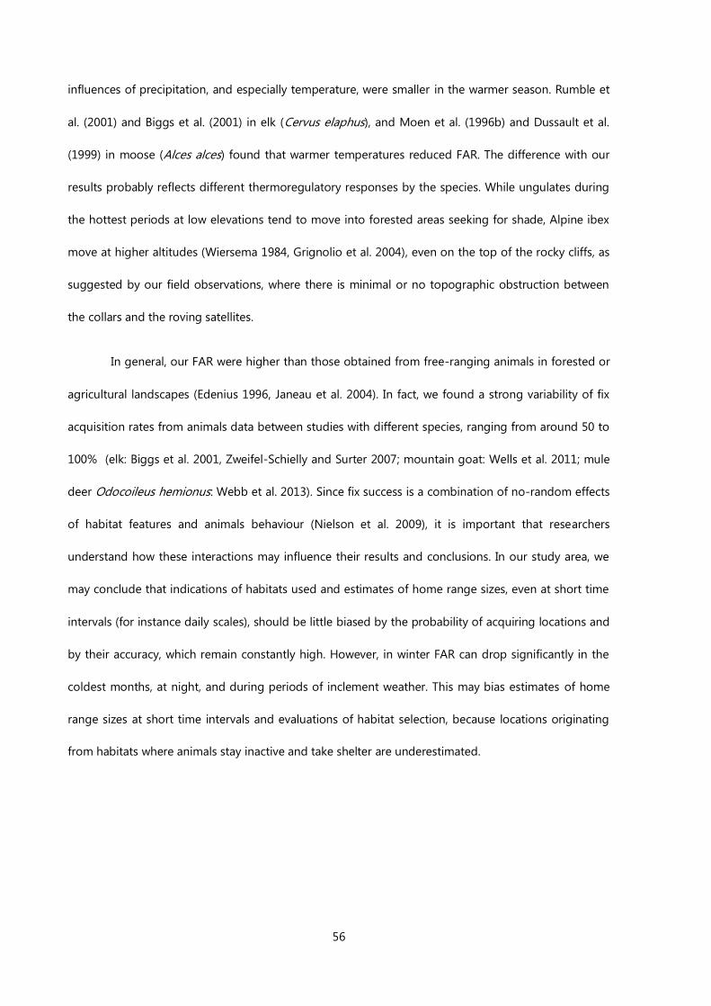
56
influences of precipitation, and especially temperature, were smaller in the warmer season. Rumble et
al. (2001) and Biggs et al. (2001) in elk (Cervus elaphus), and Moen et al. (1996b) and Dussault et al.
(1999) in moose (Alces alces) found that warmer temperatures reduced FAR. The difference with our
results probably reflects different thermoregulatory responses by the species. While ungulates during
the hottest periods at low elevations tend to move into forested areas seeking for shade, Alpine ibex
move at higher altitudes (Wiersema 1984, Grignolio et al. 2004), even on the top of the rocky cliffs, as
suggested by our field observations, where there is minimal or no topographic obstruction between
the collars and the roving satellites.
In general, our FAR were higher than those obtained from free-ranging animals in forested or
agricultural landscapes (Edenius 1996, Janeau et al. 2004). In fact, we found a strong variability of fix
acquisition rates from animals data between studies with different species, ranging from around 50 to
100% (elk: Biggs et al. 2001, Zweifel-Schielly and Surter 2007; mountain goat: Wells et al. 2011; mule
deer Odocoileus hemionus: Webb et al. 2013). Since fix success is a combination of no-random effects
of habitat features and animals behaviour (Nielson et al. 2009), it is important that researchers
understand how these interactions may influence their results and conclusions. In our study area, we
may conclude that indications of habitats used and estimates of home range sizes, even at short time
intervals (for instance daily scales), should be little biased by the probability of acquiring locations and
by their accuracy, which remain constantly high. However, in winter FAR can drop significantly in the
coldest months, at night, and during periods of inclement weather. This may bias estimates of home
range sizes at short time intervals and evaluations of habitat selection, because locations originating
from habitats where animals stay inactive and take shelter are underestimated.
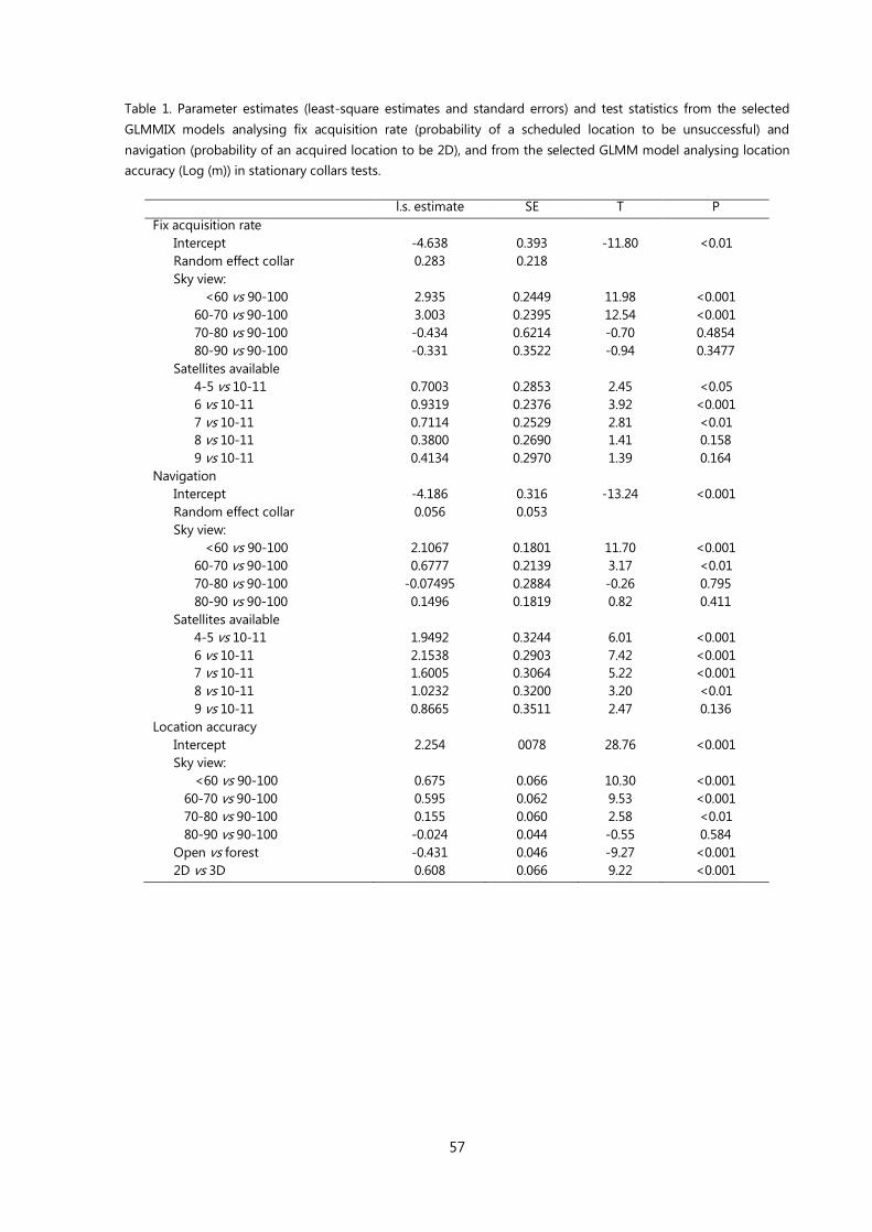
57
Table 1. Parameter estimates (least-square estimates and standard errors) and test statistics from the selected
GLMMIX models analysing fix acquisition rate (probability of a scheduled location to be unsuccessful) and
navigation (probability of an acquired location to be 2D), and from the selected GLMM model analysing location
accuracy (Log (m)) in stationary collars tests.
l.s. estimate SE T P
Fix acquisition rate
Intercept -4.638 0.393 -11.80 <0.01
Random effect collar
Sky view:
0.283 0.218
<60 vs 90-100 2.935 0.2449 11.98 <0.001
60-70 vs 90-100 3.003 0.2395 12.54 <0.001
70-80 vs 90-100 -0.434 0.6214 -0.70 0.4854
80-90 vs 90-100 -0.331 0.3522 -0.94 0.3477
Satellites available
4-5 vs 10-11 0.7003 0.2853 2.45 <0.05
6 vs 10-11 0.9319 0.2376 3.92 <0.001
7 vs 10-11 0.7114 0.2529 2.81 <0.01
8 vs 10-11 0.3800 0.2690 1.41 0.158
9 vs 10-11 0.4134 0.2970 1.39 0.164
Navigation
Intercept -4.186 0.316 -13.24 <0.001
Random effect collar
Sky view:
0.056 0.053
<60 vs 90-100 2.1067 0.1801 11.70 <0.001
60-70 vs 90-100 0.6777 0.2139 3.17 <0.01
70-80 vs 90-100 -0.07495 0.2884 -0.26 0.795
80-90 vs 90-100 0.1496 0.1819 0.82 0.411
Satellites available
4-5 vs 10-11 1.9492 0.3244 6.01 <0.001
6 vs 10-11 2.1538 0.2903 7.42 <0.001
7 vs 10-11 1.6005 0.3064 5.22 <0.001
8 vs 10-11 1.0232 0.3200 3.20 <0.01
9 vs 10-11 0.8665 0.3511 2.47 0.136
Location accuracy
Intercept 2.254 0078 28.76 <0.001
Sky view:
<60 vs 90-100 0.675 0.066 10.30 <0.001
60-70 vs 90-100 0.595 0.062 9.53 <0.001
70-80 vs 90-100 0.155 0.060 2.58 <0.01
80-90 vs 90-100 -0.024 0.044 -0.55 0.584
Open vs forest -0.431 0.046 -9.27 <0.001
2D vs 3D 0.608 0.066 9.22 <0.001

58
Table 2. Parameter estimates (least-square estimates and standard errors) and test statistics from the selected
GLMMIX models analysing fix acquisition rate (probability of a scheduled location to be unsuccessful). Night: 23
pm-02 am; Deep night: 03 am-06 am; Morning: 07 am-10 am; Midday: 11 am-14 pm; Afternoon: 15 pm-18 pm;
Evening: 19 pm-22 pm.
l.s. estimate SE T P
Su
mm
er
Random effect individual 0.169 0.077
Random effect year 0.034 0.315
Intercept -2.467 0.1783 -13.81 <0.01
Month:
June vs November 0.470 0.112 4.21 <0.001
July vs November 0.718 0.111 6.47 <0.001
August vs November 0.268 0.107 2.50 <0.05
September vs November 0.284 0.096 2.97 <0.01
October vs November -0.116 0.080 -1.44 0.151
Day period
Deep Night vs Night 0.001 0.075 0.01 0.989
Morning vs Night 0.167 0.074 2.96 <0.05
Midday vs Night 0.305 0.072 4.23 <0.001
Afternoon vs Night -0.098 0.089 -1.08 0.274
Evening vs Night -0.067 0.073 -0.09 0.923
Sky view -- -- -- --
Slope 0.316 0.025 12.59 <0.001
Activity
Average vs low -0.775 0.049 -15.91 <0.001
High vs low -2.476 0.096 -25.69 <0.001
Precipitation
no vs yes -0.532 0.052 -10.14 <0.001
Temperature -0.155 0.030 -5.23 <0.001
Win
ter
Random effect individual 0.642 0.288
Random effect year 0.041 0.040
Intercept -1.039 0.289 13.59 0.173
Month:
January vs December 0.116 0.209 0.55 0.579
February vs December -0.106 0.210 -0.51 0.613
March vs December -0.433 0.209 -2.06 0.039
April vs December -1.484 0.215 -6.90 <0.001
May vs November -1.221 0.214 -5.70 <0.001
Day period
Deep Night vs Night -0.205 0.050 -4.13 <0.001
Morning vs Night -1.103 0.069 -15.97 <0.001
Midday vs Night -1.688 0.089 -19.00 <0.001
Afternoon vs Night -0.952 0.069 -13.87 <0.001
Evening vs Night -0.112 0.049 -4.13 <0.001
Forest proportion
Average vs low 0.125 0.047 2.65 <0.01
High vs low 0.078 0.061 1.27 0.204
Sky view -0.040 0.018 -2.22 <0.05
Slope -- -- -- --
Activity
Average vs low -0.682 0.041 -16.78 <0.001
High vs low -2.371 0.131 -18.09 <0.001
Precipitation
no vs yes -0.336 0.039 -8.73 <0.001
Temperature -0.286 0.018 -15.67 <0.001

59
Table 3: Parameter estimates (least-square estimates and standard errors) and test statistics from the selected
GLMMIX models analysing navigation (probability of an acquired location to be 2D) in ibex tests. Night: 23 pm-02
am; Deep night: 03 am-06 am; Morning: 07 am-10 am; Midday: 11 am-14 pm; Afternoon: 15 pm-18 pm; Evening:
19 pm-22 pm.
l.s. estimate SE T P
Su
mm
er
Random effect individual 0.376 0.183
Random effect year 0.037 0.052
Intercept -2.356 0.226 -10.41 <0.01
Month:
June vs November 0.444 0.092 4.85 <0.001
July vs November 0.464 0.091 5.08 <0.001
August vs November 0.346 0.082 4.24 <0.001
September vs November 0.232 0.079 2.92 <0.01
October vs November 0.055 0.065 0.84 0.399
Day period
Deep Night vs Night 0.253 0.058 4.33 <0.001
Morning vs Night 0.356 0.057 6.14 <0.001
Midday vs Night 0.311 0.058 5.32 <0.001
Afternoon vs Night 0.153 0.063 2.43 <0.05
Evening vs Night -0.059 0.061 -0.97 0.331
Sky view -0.282 0.022 -12.57 <0.001
Slope -- -- -- --
Activity
Average vs low -0.321 0.041 -7.88 <0.001
High vs low -0.769 0.048 -16.01 <0.001
Precipitation
no vs yes -0.285 0.037 -7.73 <0.001
Temperature -0.095 0.021 -4.42 <0.001
Win
ter
Random effect individual 0.556 0.246
Random effect year 0.008 0.011
Intercept -1.094 0.240 -4.55 0.138
Month:
January vs December 0.073 0.106 0.69 0.493
February vs December 0.003 0.107 0.03 0.979
March vs December -0.392 0.107 -3.68 <0.001
April vs December -0.708 0.108 -6.58 <0.001
May vs November -0.601 0.108 -5.57 <0.001
Day period
Deep Night vs Night -0.141 0.052 -2.69 <0.01
Morning vs Night -0.937 0.064 -14.58 <0.001
Midday vs Night -1.025 0.067 -15.38 <0.001
Afternoon vs Night -0.219 0.058 -3.81 <0.001
Evening vs Night 0.159 0.050 3.16 <0.01
Forest proportion
Average vs low -- -- -- --
High vs low -- -- -- --
Sky view -0.122 0.017 -7.07 <0.001
Slope -- -- -- --
Activity
Average vs low -0.579 0.039 -14.09 <0.001
High vs low -0.812 0.058 -14.09 <0.001
Precipitation
no vs yes -0.343 0.036 -9.57 <0.01
Temperature -0.191 0.017 -10.91 <0.001

60
Appendix table I. Model selection for fix acquisition rate (FAR), navigation and accuracy (LE) in stationary collars.
Model Sky view Land cover
Satellites
available Day period Navigation AIC Δ AIC
FAR
1 <0.001 0.460 <0.01 -- -- 1360.0 2.7
2 <0.001 0.447 -- <0.01 -- 1358.8 1.5
3 <0.001 -- <0.001 -- -- 1358.6 1.3
4 <0.001 -- -- <0.01 -- 1357.3 0
Navigation
1 <0.001 0.117 <0.001 -- -- 1700.7 0
2 <0.001 0.099 -- <0.001 -- 1743.3 42.6
3 <0.001 -- <0.001 -- 1701.2 0.5
4 <0.001 -- -- <0.001 -- 1744.1 43.4
LE
1 <0.001 <0.001 0.207 -- <0.001 6351.0 5.7
2 <0.001 <0.001 -- 0.455 <0.001 6362.0 16.7
3 <0.001 <0.001 -- -- <0.001 6345.3 0

61
Appendix table II. Model selection for fix acquisition rate (FAR) and Navigation in the test with free-ranging ibex
Month
Day
period
Land
cover Sky view Slope Activity precipitation Temperature Snow AIC ΔAIC
FA
R
Summer
1 <0.001 <0.001 0.442 <0.001 -- <0.001 <0.001 <0.001 -- 15793.63 42.03
2 <0.001 <0.001 0.867 -- <0.001 <0.001 <0.001 <0.001 -- 15755.30 3.7
3 <0.001 <0.001 -- <0.001 -- <0.001 <0.001 <0.001 -- 15791.25 39.65
4 <0.001 <0.001 -- -- <0.001 <0.001 <0.001 <0.001 -- 15751.60 0
Winter
1 <0.001 <0.001 <0.05 <0.05 -- <0.001 <0.001 <0.001 0.129 22026.11 0
2 <0.001 <0.001 <0.05 -- 0.225 <0.001 <0.001 <0.001 0.179 22030.30 4.19
3 <0.001 <0.001 <0.05 <0.05 -- <0.001 <0.001 <0.001 -- 22026.42 0.31
4 <0.001 <0.001 <0.05 -- 0.2648 <0.001 <0.001 <0.001 -- 22030.10 3.99
5 <0.001 <0.001 <0.05 -- -- <0.001 <0.001 <0.001 22029.30 3.19
6 <0.001 <0.001 -- <0.05 -- <0.001 <0.001 <0.001 -- 22029.64 3.53
7 <0.001 <0.001 -- -- -- <0.001 <0.001 <0.001 22032.62 6.51
Navig
ati
on
Summer
1 <0.001 <0.001 0.170 <0.001 -- <0.001 <0.001 <0.001 -- 25502.00 0.44
2 <0.001 <0.001 0.112 -- <0.001 <0.001 <0.001 <0.001 -- 25567.44 65.88
3 <0.001 <0.001 -- <0.001 -- <0.001 <0.001 <0.001 -- 25501.56 0
4 <0.001 <0.001 -- -- <0.001 <0.001 <0.001 <0.001 -- 25567.70 66.14
Winter
1 <0.001 <0.001 0.060 <0.001 -- <0.001 <0.001 <0.001 0.370 25353.89 0
2 <0.001 <0.001 0.067 -- <0.05 <0.001 <0.001 <0.001 0.098 25396.51 42.62
3 <0.001 <0.001 0.061 <0.001 -- <0.001 <0.001 <0.001 -- 25532.69 178.8
4 <0.001 <0.001 0.069 -- <0.05 <0.001 <0.001 <0.001 25397.27 43.38
5 <0.001 <0.001 -- <0.001 -- <0.001 <0.001 <0.001 -- 25354.29 0.4
6 <0.001 <0.001 -- -- <0.05 <0.001 <0.001 <0.001 -- 25398.63 44.74

62
0.4
0.5
0.6
0.7
0.8
0.9
1
1.1
1.2
<60
60-70
70-80
80-90
90-100
4-5
6
7
8
9
10-11
Skyview Satellitesavailable
3D/A
cquired
0.4
0.5
0.6
0.7
0.8
0.9
1
1.1
1.2
<60
60-70
70-80
80-90
90-100
4-5
6
7
8
9
10-11
Skyview Satellitesavailable
Acquired
/sched
uled
Figure 1: proportion of acquired over scheduled locations for the different sky view and available satellites classes.
Values are means of location points within classes. Vertical bars indicate SD.
Figure 2: proportion of locations over acquired locations for the different sky view and available satellites classes.
Values are means of location points within classes. Vertical bars indicate SD.

63
0.6
0.7
0.8
0.9
1
1.1
June
July
August
September
October
November
December
January
February
March
April
May
Summer Winter
Acquired
/sched
uled
Figure 3: Accuracy (distance from true location, m) within different sky view classes and land use and navigation
categories. Box plots comprise the 25th
and 75th
quintiles, while vertical bars indicate the 10th
and the 90th
quintiles.
Figure 4: proportion of acquired over scheduled locations in the various seasons and months with ibex tests.
Values are means of individual female ibex. Vertical bars represent SD.

64
0.6
0.7
0.8
0.9
1
1.1
June
July
August
September
October
November
December
January
February
March
April
May
Summer Winter
3D/acquired
Figure 5: proportion of acquired over scheduled locations in the various seasons and day periods with ibex tests.
Values are means of individual female ibex. Vertical bars represent SD. Night: 23 pm-02 am; Deep night: 03 am-06
am; Morning: 07 am-10 am; Midday: 11 am-14 pm; Afternoon: 15 pm-18 pm; Evening: 19 pm-22 pm.
Figure 6: proportion of 3D over acquired locations in the various seasons and months with ibex tests. Values are
means of individual female ibex. Vertical bars represent SD.
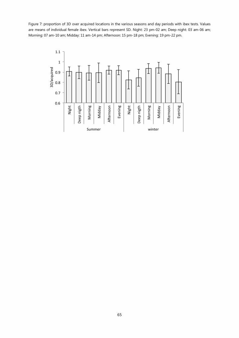
65
Figure 7: proportion of 3D over acquired locations in the various seasons and day periods with ibex tests. Values
are means of individual female ibex. Vertical bars represent SD. Night: 23 pm-02 am; Deep night: 03 am-06 am;
Morning: 07 am-10 am; Midday: 11 am-14 pm; Afternoon: 15 pm-18 pm; Evening: 19 pm-22 pm.

66
LITERATURE CITED
Adrados, C., Girard, I., Gendner, J. P., and Janeau, G. (2002). Global positioning system (GPS) location
accuracy improvement due to selective availability removal. Comptes Rendus Biologies, 325(2), 165-
170.
Biggs, J. R., Bennett, K. D., and Fresquez, P. R. (2001). Relationship between home range characteristics
and the probability of obtaining successful global positioning system (GPS) collar positions for elk in
New Mexico. Western North American Naturalist, 61(2), 213-222.
Bourgoin, G., Garel, M., Dubray, D., Maillard, D., and Gaillard, J. M. (2009). What determines global
positioning system fix success when monitoring free-ranging mouflon?. European journal of wildlife
research, 55(6), 603-613.
Bozdogan, H. (1987). Model selection and Akaike's information criterion (AIC): The general theory and
its analytical extensions. Psychometrika, 52(3), 345-370.
Cagnacci, F., Boitani, L., Powell, R. and Boyce, M. (2010) Animal ecology meets GPS-based
radiotelemetry: a perfect storm of opportunities and challenges. Phil. Trans. R. Soc. B 365, 2157-2162.
(doi:1098/rstb.2010.0107).
Cain III, J. W., Krausman, P. R., Jansen, B. D. and Morgart, J. R. (2005) Influence of topography and GPS
fix interval on GPS collar performance. Wildlife Soc. B 33, 926-934.
Cargnelutti, B., Coulon, A., Hewison, A. J., Goulard, M., ANGIBAULT, J., and Morellet, N. (2007). Testing
Global Positioning System performance for wildlife monitoring using mobile collars and known
reference points. The Journal of wildlife management, 71(4), 1380-1387.
Clutton-Brock, T. H., and Vincent, A. C. (1991). Sexual selection and the potential reproductive rates of
males and females. Nature, 351(6321), 58-60.
Cooke, S. J., Hinch, S. G., Wikelski, M., Andrews, R. D., Kuchel, L. J., Wolcott, T. G. and Butler, P. J. (2004).
Biotele-metry: a mechanistic approach to ecology. Trends Ecol. Evol. 19, 334 – 343.
Danilkin, A. A., & Hewison, A. M. (1996). Behavioural ecology of Siberian and European roe deer.
DeCesare, N. J., Squires, J. R., and Kolbe, J. A. (2005). Effect of forest canopy on GPS-based movement
data. Wildlife Society Bulletin, 33(3), 935-941.
Deckert, C., and Bolstad, P. V. (1996). Forest canopy, terrain, and distance effects on global positioning
system point accuracy. Photogrammetric Engineering and Remote Sensing, 62(3), 317-321.
D'Eon, R. G. (2003). Effects of a stationary GPS fix-rate bias on habitat-selection analyses. The Journal
of Wildlife Management, 858-863.
D'Eon, R. G., and Delparte, D. (2005). Effects of radio‐collar position and orientation on GPS radio‐collar
performance, and the implications of PDOP in data screening. Journal of Applied Ecology, 42(2), 383-
388.
D'Eon, R. G., Serrouya, R., Smith, G., and Kochanny, C. O. (2002). GPS radiotelemetry error and bias in
mountainous terrain. Wildlife Society Bulletin, 430-439.
Duprè E., Pedrotti L. and Arduino S. (2001) Alpine ibex conservation strategy. The Alpine ibex in the
Italian Alps: status, potential distribution and management options for conservation and sustainable
development. Available online at: http://biocenosi.dipbsf.uninsubria.it/LHI/

67
Dussault, C., Courtois, R., Ouellet, J. P., and Huot, J. (1999). Evaluation of GPS telemetry collar
performance for habitat studies in the boreal forest. Wildlife Society Bulletin, 965-972.
Edenius, L., and Elmberg, J. (1996). Landscape level effects of modern forestry on bird communities in
North Swedish boreal forests. Landscape Ecology, 11(6), 325-338.
Frair, J. L., Nielsen, S. E., Merrill, E. H., Lele, S. R., Boyce, M. S., Munro, R. H., ... and Beyer, H. L. (2004).
Removing GPS collar bias in habitat selection studies. Journal of Applied Ecology, 41(2), 201-212.
Fuller, M. R., Millspaugh, J. J., Church, K. E. and Kenward, R. E. (2005). Wildlife radio telemetry. In
Techniques for wild-life investigations and management (ed. C. E. Braun), 6th ed., pp. 377– 417.
Bethesda, MD: The Wildlife Society.
Gamo, R. S., Rumble, M. A., Lindzey, F., and Stefanich, M. (2000). GPS radio collar 3D performance as
influenced by forest structure and topography. Biotelemetry, 15, 464-473.
Girard, I., Adrados, C., Peracino, A., Marinot, J. P., Bassano, B., and Janeau, G. (2002). Feasibility of GPS
use to locate wild ungulates in high mountain environment. Pirineos, 157, 7-14.
Glasby, L., and Yarnell, R. W. (2013). Evaluation of the performance and accuracy of Global Positioning
System bug transmitters deployed on a small mammal. European Journal of Wildlife Research, 59(6),
915-919.
Graves, T. A., and Waller, J. S. (2006). Understanding the causes of missed global positioning system
telemetry fixes. Journal of Wildlife Management, 70(3), 844-851.
Grignolio, S., Parrini, F., Bassano, B., Luccarini, S., and Apollonio, M. (2003). Habitat selection in adult
males of Alpine ibex, Capra ibex ibex. Folia Zoologica, 52(2), 113-120.
Grignolio, S., Rossi, I., Bassano, B., Parrini, F., and Apollonio, M. (2004). Seasonal variations of spatial
behaviour in female Alpine ibex (Capra ibex ibex) in relation to climatic conditions and age. Ethology
Ecology and Evolution, 16(3), 255-264.
Grignolio, S., Rossi, I., Bassano, B., and Apollonio, M. (2007). Predation risk as a factor affecting sexual
segregation in Alpine ibex. Journal of Mammalogy, 88(6), 1488-1497.
Guthrie, J. D., Byrne, M. E., Hardin, J. B., Kochanny, C. O., Skow, K. L., Snelgrove, R. T., ... and Collier, B. A.
(2011). Evaluation of a Global Positioning System backpack transmitter for wild turkey research. The
Journal of Wildlife Management, 75(3), 539-547.
Handcock, R.N., Swain, D.L., Bishop-Hurley, G.J., Patison, K.P., Wark, T., Valencia, P., Corke, P. and
O’Neill, C. . (2009). Monitoring animal behaviour and environmental interactions using wireless sensor
networks, GPS collars and satellite remote sensing. Sensors 9, 3586-3603.
Hansen, M. C., and Riggs, R. A. (2008). Accuracy, precision, and observation rates of global positioning
system telemetry collars. The Journal of Wildlife Management, 72(2), 518-526.
Heard, D. C., Ciarniello, L. M., and Seip, D. R. (2008). Grizzly bear behavior and global positioning
system collar fix rates. The Journal of Wildlife Management, 72(3), 596-602.
Hebblewhite, M., PERCY, M. and MERRILL, E. H. (2007), Are All Global Positioning System Collars
Created Equal? Correcting Habitat-Induced Bias Using Three Brands in the Central Canadian Rockies.
The Journal of Wildlife Management, 71: 2026–2033.
Hulbert, I. A., and French, J. (2001). The accuracy of GPS for wildlife telemetry and habitat mapping.
Journal of Applied Ecology, 38(4), 869-878.

68
Janeau, G., Adrados, C., Joachim, J., Gendner, J. P., and Pépin, D. (2004). Performance of differential GPS
collars in temperate mountain forest. Comptes rendus biologies, 327(12), 1143-1149.
Jiang, Z., Sugita, M., Kitahara, M., Takatsuki, S., Goto, T., and Yoshida, Y. (2008). Effects of habitat
feature, antenna position, movement, and fix interval on GPS radio collar performance in Mount Fuji,
central Japan. Ecological Research, 23(3), 581-588.
Lewis, J. S., Rachlow, J. L., Garton, E. O., and Vierling, L. A. (2007). Effects of habitat on GPS collar
performance: using data screening to reduce location error. Journal of Applied Ecology, 44(3), 663-671.
Matthews, A., Ruykys, L., Ellis, B., FitzGibbon, S., Lunney, D., Crowther, M. S., ... and Wiggins, N. (2013).
The success of GPS collar deployments on mammals in Australia. Australian Mammalogy, 35(1), 65-83.
Moen, R., Pastor, J., and Cohen, Y. (1997). Accuracy of GPS telemetry collar locations with differential
correction. The Journal of wildlife management, 530-539.
Moen, R., Pastor, J., Cohen, Y. and Schwartz C.C. (1996). Effects of moose movement and habitat use on
GPS collar performance. Journal of Wildlife Management 63:659-668.
Moen, R., Pastor, J., & Cohen, Y. (2001). Effects of animal activity on GPS telemetry location attempts.
Alces, 37(1), 207-216.
Morellet, N., Bonenfant, C., Börger, L., Ossi, F., Cagnacci, F., Heurich, M., ... & Mysterud, A. (2013).
Seasonality, weather and climate affect home range size in roe deer across a wide latitudinal gradient
within Europe. Journal of animal ecology, 82(6), 1326-1339.
Nielson, R. M., Manly, B. F., McDonald, L. L., Sawyer, H., and McDonald, T. L. (2009). Estimating habitat
selection when GPS fix success is less than 100%. Ecology, 90(10), 2956-2962.
Pepin, D., Joachim, J., and Ferrié, E. (1996). Variability of spring selection by isards (Rupicapra
pyrenaica). Can. J. Zool, 75, 1955-1965.
Quaglietta, L., Martins, B. H., de Jongh, A., Mira, A., and Boitani, L. (2012). A low-cost GPS GSM/GPRS
telemetry system: performance in stationary field tests and preliminary data on wild otters (Lutra lutra).
PloS one, 7(1), e29235.
Rempel, R. S., and Rodgers, A. R. (1997). Effects of differential correction on accuracy of a GPS animal
location system. The Journal of Wildlife Management, 525-530.
Rettie, W. J., and McLoughlin, P. D. (1999). Overcoming radiotelemetry bias in habitat-selection studies.
Canadian Journal of Zoology, 77(8), 1175-1184.
Rossi, I., Lamberti, P., Mauri, L., & Apollonio, M. (2003). Home range dynamics of male roe deer
Capreolus capreolus in a mountainous habitat. Acta theriologica, 48(3), 425-432.
Rumble, M. A. and Lindzey, F. (1997). Effects of forest vegetation and topography on global positioning
system collars for elk. Pages 492 – 501 in: American Society for Photogrammetry and Remote Sensing,
American Congress on Surveying and Mapping, Annual Convention and Exposition Technical Papers,
Vol. 4. Resource Technology Institute, Seattle, Washington, USA.
Sager‐Fradkin, K. A., Jenkins, K. J., Hoffman, R. A., Happe, P. J., Beecham, J. J., and Wright, R. G. (2007).
Fix Success and Accuracy of Global Positioning System Collars in Old‐Growth Temperate Coniferous
Forests. The Journal of wildlife management, 71(4), 1298-1308.
Schielzeth, H. (2010) Simple means to improve the interpretability of regression coefficients. Methods
in Ecology and Evolution, 1, 103–113.

69
Scillitani L., Sturaro E., Menzano A., Rossi L., Viale C., Ramanzin M. (2012). Post-release spatial and
social behaviour of translocated male Alpine ibexes (Capra ibex ibex) in the eastern Italian Alps. Eur J
Wildl Res., 58: 461–472.
Scillitani L., Sturaro ., Onaco E., Rosi L., Ramanzin M. (2012). Factors affecting home range size of male
Alpine ibex (Capra ibex ibex) in the Marmolada massif. Hystrix-It. J. Zool. Doi: 10.4404/hystrix-23.2-
4622.
Scillitani L., Darmon G., Moncao A., Cocca G., Sturaro E., Rossi L., Ramanzin M. (2013). Habitat selection
in translocated gregarious ungulate species: an interplay between sociality and ecological
requirements. J. Wildl. Manag. 77: 761-769.
Signer, C., Ruf, T., & Arnold, W. (2011). Hypometabolism and basking: the strategies of Alpine ibex to
endure harsh over‐wintering conditions. Functional Ecology, 25(3), 537-547.
Tomkiewicz, S. M., Fuller, M. R., Kie, J. G., and Bates, K. K. (2010). Global positioning system and
associated technologies in animal behaviour and ecological research. Philosophical Transactions of the
Royal Society B: Biological Sciences, 365(1550), 2163-2176.
Villaret, J. C., Bon, R., and Rivet, A. (1997). Sexual segregation of habitat by the alpine ibex in the French
Alps. Journal of Mammalogy, 1273-1281.
Villepique, J. T., Bleich, V. C., Pierce, B. M., Stephenson, T. R., Botta, R. A., and Bowyer, R. T. (2008).
Evaluating GPS collar error: a critical evaluation of Televilt POSREC-Science (TM) collars and a method
for screening location data. California Fish and Game, 94(4), 155-168.
Wiersema, G. (1984). Seasonal use and quality assessment of ibex habitat. Acta Zoologica
Fennica[ACTA ZOOL. FENN.]. 1984.
Webb, S. L., Dzialak, M. R., Mudd, J. P., & Winstead, J. B. (2013). Developing spatially-explicit weighting
factors to account for bias associated with missed GPS fixes in resource selection studies. Wildlife
Biology, 19(3), 257-273.
Williams, D. M., Quinn, A. D., and Porter, W. F. (2012). Impact of habitat-specific GPS positional error on
detection of movement scales by first-passage time analysis. PloS one, 7(11), e48439.
Wells, A. G., Wallin, D. O., Rice, C. G., and Chang, W. Y. (2011). GPS bias correction and habitat selection
by mountain goats. Remote Sensing, 3(3), 435-459.
Zweifel-Schielly, B., and Suter, W. (2007). Performance of GPS telemetry collars for red deer Cervus
elaphus in rugged Alpine terrain under controlled and free-living conditions. Wildlife Biology, 13(3),
299-312.


71
CHAPTER 2
DETERMINANTS OF HOME RANGE SIZE ACROSS
SPATIO-TEMPORAL SCALES IN A HIGH MOUNTAIN
UNGULATE
PARRAGA M.A., STURARO E., ROSSI L.1, RAMANZIN M.
1 Dipartimento di Scienze Veterinarie, Università di Torino


73
INTRODUCTION
Patterns of space use by animals reflect their responses to habitats and climate variations
(Johnson et al. 1992, Morales et al. 2004, Fieberg et al. 2010, Tomkiewicz et al. 2010), and may
influence individual performance and population dynamics (Gaillard et al. 2010, Morales et al. 2010,
Spencer 2012). A concept widely used to describe animal space use is the home range (HR), which
defines the areas used with different intensities and frequencies by an individual in search of food,
shelter and mates (Börger, Dalziel and Fryxell 2008). The HR concept has greatly evolved during the
last decades (Burt 1943, Powell 2000, Gaillard et al. 2010, Kie et al. 2010, Powell and Mitchell, 2012),
especially after the advent of GPS tracking technologies that allow to describe movement at very
detailed spatio-temporal scales (Börger et al. 2008; Kie et al. 2010, Benhamou and Riotte-Lambert
2012). However, in principle the size of a HR reflects how an individual is able to satisfy its needs in
relation to the available resources. Therefore, understanding why HR size varies among and within
species has received and continues to receive widespread consideration in ecology research (see
reviews in Börger, Dalziel and Fryxell 2008; Kie et al. 2010; Moorcroft, 2012, Potts and Lewis 2014).
Among terrestrial mammal species, body mass, being an index of the energy needs and movement
capability of animals, is the main determinant of HR size, with type of food playing a significant but
lower role (McNab, 1963; Harestad and Bunnell, 1979, Tucker et al., 2014). Within species, the HR size
of large herbivores may be affected by several factors, such as population density (Vincent et al. 1995,
Kjellander et al. 2004), forage availability (Bremset Hansen et al. 2009, Owen-Smith et al. 2010), human
disturbance (Creel et al. 2002, Manor and Saltz 2003), climatic conditions (Jacobson et al. 2004, Floris et
al. 2012), or individual status (Green 1992, Dahle and Swenson 2003, Said et al. 2005). However, studies
attempting to examine in a single analysis the range of extrinsic and intrinsic factors affecting HR size
are very few (see van Beest et al. 2011 for moose Alces alces and Borger et al. 2006 and Morellet et al.
2013 for roe deer Capreolus capreolus). These studies suggested that, in temperate regions, the HR
size of large herbivores follows predictable intra-annual patterns in response to seasonality of climatic
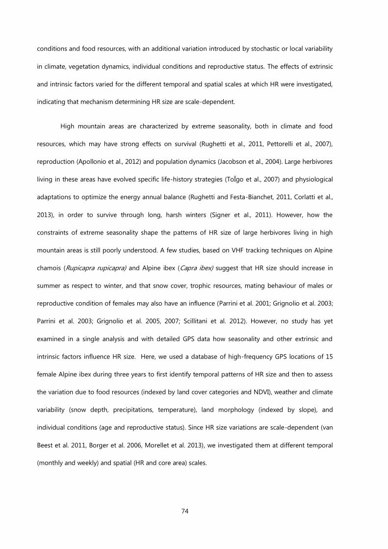
74
conditions and food resources, with an additional variation introduced by stochastic or local variability
in climate, vegetation dynamics, individual conditions and reproductive status. The effects of extrinsic
and intrinsic factors varied for the different temporal and spatial scales at which HR were investigated,
indicating that mechanism determining HR size are scale-dependent.
High mountain areas are characterized by extreme seasonality, both in climate and food
resources, which may have strong effects on survival (Rughetti et al., 2011, Pettorelli et al., 2007),
reproduction (Apollonio et al., 2012) and population dynamics (Jacobson et al., 2004). Large herbivores
living in these areas have evolved specific life-history strategies (ToÏgo et al., 2007) and physiological
adaptations to optimize the energy annual balance (Rughetti and Festa-Bianchet, 2011, Corlatti et al.,
2013), in order to survive through long, harsh winters (Signer et al., 2011). However, how the
constraints of extreme seasonality shape the patterns of HR size of large herbivores living in high
mountain areas is still poorly understood. A few studies, based on VHF tracking techniques on Alpine
chamois (Rupicapra rupicapra) and Alpine ibex (Capra ibex) suggest that HR size should increase in
summer as respect to winter, and that snow cover, trophic resources, mating behaviour of males or
reproductive condition of females may also have an influence (Parrini et al. 2001; Grignolio et al. 2003;
Parrini et al. 2003; Grignolio et al. 2005, 2007; Scillitani et al. 2012). However, no study has yet
examined in a single analysis and with detailed GPS data how seasonality and other extrinsic and
intrinsic factors influence HR size. Here, we used a database of high-frequency GPS locations of 15
female Alpine ibex during three years to first identify temporal patterns of HR size and then to assess
the variation due to food resources (indexed by land cover categories and NDVI), weather and climate
variability (snow depth, precipitations, temperature), land morphology (indexed by slope), and
individual conditions (age and reproductive status). Since HR size variations are scale-dependent (van
Beest et al. 2011, Borger et al. 2006, Morellet et al. 2013), we investigated them at different temporal
(monthly and weekly) and spatial (HR and core area) scales.

75
In particular, we hypothesized that:
H1. Due to the extreme seasonality of high mountain areas, HR should follow an intra-annual
pattern at all temporal and spatial scales, and particularly that (H1a) HR size should decrease during
autumn and winter, and increase during spring and summer (Gross et al. 2002, van Beest 2011), due to
the strong limitations to movement imposed by deep snow (Rossi et al. 2003, Grignolio et al. 2003)
and the marked energy-saving behaviour of Alpine ibex in winter (Signer et al. 2011). Since daylight is
directly related with the predictability of climate and resource availability, we expected (H1b) that HR
size was positively correlated with photoperiod, in contrast to the negative correlation found in other
species inhabiting lower altitudes with milder winter and higher forage availabilities (Borger et al. 2006,
Saïd et al. 2005, Morellet et al. 2013), and that (H1c) cyclic intra-annual trends in climate (indexed by
average daily temperature) and forage availability (indexed by NDVI of study area, Hamel et al. 2009)
might exert further influence on HR size patterns.
H2 We expected that spatiotemporal stochastic variations in climate and food resources had a
strong influence on HR size (van Beest et al. 2011; Saïd et al. 2005, 2009). In particular, we predicted
that in winter (H2a) HR size decreased with increase in snow depth (Grignolio et al. 2003) and in
periods of high precipitations (H2b) and low temperatures (H2c), due to reduced mobility and energy
saving behaviour of ibex in such conditions (Grøtan et al. 2007, Signer and Arnold 2008). In summer
(H2d), we expected low or no effects of precipitations or temperature, although high temperatures
might induce a greater mobility in search of cooler areas. According to the energy needs theory, we
predicted that (H2e) HR size should decrease with increase in food resources (Aublet and Festa-
Bianchet 2009, Owen-Smith et al. 2010), which we indexed with the proportion of vegetation as
respect to bare ground (Scillitani et al., 2012), but also with NDVI (Bremset Hansen et al. 2009, Mueller
et al. 2011).
H3. Steep slopes are the predominant landscape feature in the study area and the habitat
preferred by ibex when searching for shelter during the weaning period, for refuge to warm

76
temperatures in summer and for shallower snow patches during winter (Gross et al. 2002, Grignolio et
al. 2004). Therefore we predicted that (H3a) HR sizes may decrease when increase in the degree of the
occupied slopes (Scillitani et al. 2012).
H4. The individual age and reproductive status may influence the space use by females in
different ways. We expected that young females might show (H4a) larger HR than older females due to
social and spatial instability, as suggested by Grignolio et al. (2004). Females with offspring have been
found to have either larger (Cederlund and Sand 1994, Saïd et al. 2005) or smaller (van Beest et al.
2011) HR than barren females. In response to the reduced mobility hypothesis, we expected (H4b) that
non-lactating females had larger HR than lactating females (Grignolio et al. 2007). However, given the
gregariousness of Alpine ibex females, we also predicted (H4c) that the effects of reproductive status
were much less marked than those found in non-gregarious species (van Beest 2011).
MATERIAL AND METHODS
Study area
The Marmolada massif is the highest mountain group in the Dolomites area and is located in
the eastern Italian Alps (see Scillitani et al. 2012 for details). It is characterized by a complex
topography with several summits around 3.000 m a .s.l. It is possible to identify two main boundaries
corresponding to different landscapes: the north-western, which is composed by gentle slopes and
open valleys, and the south-eastern side, where vertical rock walls up to 1.000 m of height, high
ruggedness, and deep valleys shape the environment. The vegetation in the areas used by ibex (from
1.491 m to 3.261 m in elevation) is clearly stratified, from isolated shrubs and alpine grasslands at
higher altitudes to alpine forests dominated by species of the genus Larix at the lowest one,.

77
Animals and tracking
GPS locations were collected from September 2010 to October 2013 from 15 females of Alpine
ibex (estimated age ranged from 2 to 12 years). Animals were captured during the summer seasons,
from July to early October, with veterinary assistance in compliance with current Italian laws, using a
tele-injection of xylazine (Rompun©, Bayer, Leverkusen, Germany). All captured individuals were aged
from horn annuli growth and examined for general health condition. Reproduction status was assessed
from udder morphology and presence of milk, and confirmed by visual observations of mother-kid
associations in the period immediately following the release, and in the following summers of
monitoring. The individuals were marked with colored and numbered ear tags and equipped with GPS-
GSM Plus collars (Vectronic Aerospace GmbH). Collars were scheduled to attempt to record an animal
location every 1 hour during 54 weeks. Data were received on a GSM Ground Station and downloaded
and processed using a specific software (GPS Plus Collar Manager© 3.11.3, Vectronic Aerospace
GmbH).
Data editing and calculation of Home Range sizes
We identified largely erroneous positions as “outliers” data with the screening method
developed by Bjørneraas et al, (2010), using PgAdmin tool for PostgreSQL©
1.16.0
(http://www.pgadmin.org). After removing the outliers, we then calculated individual home ranges at a
weekly and a monthly temporal scale, setting the starting date at the 21st of December. We used a
local convex hull (LoCoH) non parametric kernel method for constructing the home range polygons,
using the adehabitat package for R (R Development Core Team 2008) as developed by Calenge (2006).
Particularly, we used the k-LoCoH approach which constructs the convex hull associated with each GPS
location and its k-1 nearest neighbors (k=√n, where n is the number of points for the corresponding
individual and annual week), representing the frequently used areas by the resulting union of hulls in
78
x% isopleths (Getz and Wilmers 2004, Getz et al. 2007). This method is appropriate when working with
species living in areas of complex topography, since it takes into account physiographical boundaries,
such lakes or rocky outcrops, which are not used by the animals. We estimated weekly and monthly
home ranges at two different spatial scales: using the 95% isopleths (hereafter called HR) and the 50%
isopleths, (hereafter called core areas, CA). We excluded weeks with less than 4 days and/or less than
72 locations, and months with less than 350 locations. We associated to each retained HR and CA the
variables described below.
Variables description
Seasons.
We used a clustering approach (Kaufman and Rousseeuw 2009) to identify biological seasons
based on movement and habitat descriptors associated with locations. The results are detailed in
“Supplementary material I”. Based on these results, we classified as “summer” the weeks from 22 to 40,
and the months from 6 to 10, and as “winter” the weeks from 41 to 52 and from 1 to 21, and the
months from 11 to 12 and from 1 to 5.
Individual variables.
Age class of the females was classified into “subadult” (≤ 3 years old) or “adult” (> 3 years
old); we set the date of age change at June 1st. Reproductive status was defined as “lactating ” or
“non-lactating” respectively. We used this classification only for summer HR and CA, since this season
covered the parturition and weaning periods.

79
Climatic variables and daylight.
Climatic data were obtained from two meteorological stations, “Monti Alti di Ornella” located
at 4.5 km from the Marmolada massif e “Passo Valles” located at 11.3 km (altitude: 2.250 m a.s.l and
2.032 m a.s.l respectively). We recorded daily snow depth to the ground (cm), total daily precipitation
(mm) and average daily temperature (°C). The variables were expressed both as absolute values and as
residuals from the average trend during the study period, to index stochastic variability. Note that
these variables express only approximately the conditions experienced by ibex, but record the
temporal trends and stochastic variations. Daylight was calculated based on the geographic
coordinates of the study area and Julian date. All variables were standardized as z-scores.
Land cover and morphology.
We used a land cover map of the study area based on a high resolution digital orthofoto
(1x1m, WGS84/UTM32) (Scillitani et al., 2012; Scillitani et al., 2013) to reclassify with ArcGIS®
10.1 (Esri
Inc., Redlands, USA) 11 different vegetation covers into 2 prevalent types: “vegetation”, combining
grasslands, shrubs and forest, and “scree and rocks”, using. We used a high resolution (5x5m) Digital
Elevation Model (Regione del Veneto, Unità di Progetto per il SIT e la cartografia, 2006.
http://idt.regione.veneto.it/app/metacatalog/) to create the slope layer of the study area. Slope values
were then grouped into 9 intervals of 10 per cent units. Once overlapped with the polygons of the HRs
and CAs, each interval class was assigned a unit score (1,2,…10), starting from the lowest class, and a
slope index was calculated as Σ(Si*Pi), where Si is the score of interval class i, and Pi is its proportion in
the polygon (HR or CA) area.
NDVI index of vegetation greenness.
We used remotely sensed data from MODIS (Moderate Resolution Imaging
Spectroradiometer, NASA TERRA satellites) that provides the NDVI satellite imagery with high

80
temporal (16-day compositing periods) and spatial resolution (250x250m) (Huete et al. 2002). To
reduce the temporal resolution we resampled the images into 7-days intervals by calculating the mean
value of each pixel between two successive images using ArcGis 10.1 (ESRI®
). Total NDVI images were
165, with a weekly temporal resolution from September 2010 to mid-October 2013. We calculated the
average value of the weekly and monthly NDVI at three spatial scales: within the entire study area, and
within the polygons (HR or CA) areas.
Statistical analysis
We log-transformed HR and CA size values, and excluded as outliers the values lying outside
the mean ± 3 SD. We had 672 HR weekly estimates (232 in summer and 440 in winter), 680 weekly CA
estimates (233 in summer and 445 in winter), and 160 monthly HR and CA estimates (64 in summer
and 96 in winter).
Temporal trends of HR and CA.
The analyses were conducted in R (Development Core Team 2008), using the mgcv and nlme
packages. We first tested for intra-annual patterns of variation of HR and CA size with generalized
additive mixed models (mgcv package, Wood 2001) models, using the week or the month, depending
on the temporal scale of analysis, as fixed covariate factors, and the individual as random factors. In
order to test the effects of daylight, NDVI and temperature (absolute) on intra-annual patterns, we
used two approaches: first, we verified whether the addition of these variables as linear terms
improved the fit of the general additive mixed models with week, using a likelihood ratio test; second,
we tested the linear relationship between HR and CA size and daylight, NDVI, and temperature using
mixed linear models (nlme package, Pinheiro et al. 2011), with individual as random factor.

81
Effects of individual, climatic and habitat variables on HR and CA size.
In order to assess the effects of individual, climatic and habitat factors, we analysed HR and CA
size within summer and winter with linear mixed models at the two temporal scales, using individual as
random factor. Fixed categorical factors used were age class, reproductive status (summer only) and
prevalent land cover class, while fixed covariate factors were daylight, absolute temperature, NDVI of
study area, NDVI of the polygons (summer only), slope index, snow stochastic variation (winter only),
temperature stochastic variation, and precipitation stochastic variation. We started from the most
complex model and then removed sequentially all factors, starting from those non-significant in order
to reach the most parsimonious model (Caswell, 1988). Model selection was based on the Akaike’s
Information Criterion index (AICc) (Zuur et al. 2009); when two models differed less than 2 in AIC value,
we selected the simpler one. We tested in alternative the covariate variables with a correlation higher
than 0.45 (see appendix tables I, II, III, IV).
RESULTS
Weekly home ranges and core areas
Weekly HR size was extremely variable (mean = 21.1 ha; SD = 27.3) as well as that of CA (mean
= 2.0 ha; SD = 3.1). Both were larger in summer (HR: mean = 37.8 ha, SD = 32.9, CA: mean = 4.3 ha, SD
= 4.1) than in winter (HR = 10.2 ha, SD = 14.4; CA: mean = 0.7 ha, SD = 0.9).
Temporal trends.
The general linear additive mixed models with week as a covariate indicated that there was a
strong intra-annual pattern for both HRs and CAs, with an increase during late winter and spring, a
peak in summer and a decline afterwards (Figure 1). However, weekly HRs peaked earlier and had

82
much less pronounced variations than weekly CAs. The addition of daylight, NDVI of study area and
absolute temperature (see figure 2 for their intra-annual trends) as linear covariates to the general
additive mixed models with week did not improve the fit of the models for HRs, as indicated by the
likelihood ratio test (daylight: P = 0.115; NDVI: P = 0.497; temperature: P = 0.227). The addition of
NDVI (P < 0.001) and temperature (P < 0.001), but not that of daylight (P = 0.514) improved the fit of
general mixed linear models for CAs. When tested singularly in mixed linear models, all the three
variables were highly significantly related to HR and CA size, but the most explicative was daylight for
HRs (daylight model: AIC = 2333.2, Δ AIC = 0; NDVI model: AIC = 2335.6, Δ AIC = 2.4; Temperature
model: AIC = 2339.4, Δ AIC = 6.2) and temperature, close to NDVI, for CAs (daylight model: AIC =
2325.9, Δ AIC = 165.9; NDVI model: AIC = 2167.8, Δ AIC = 6.8; Temperature model: AIC = 2160.0, Δ
AIC = 0).
Effects of individual, climatic and habitat variables.
The results of the selection of mixed linear models are given in Appendix table V for summer
HR and CA, and in Appendix table VI for winter HR and CA. In both seasons, the most parsimonious
models for both spatial scales did not include reproductive status, prevalent land cover, temperature
stochastic variation, and precipitations stochastic variations. In summer, age class was retained only in
the HR model. Among the temporal and climatic variables, daylight and NDVI of study area were
retained in both HR and CA models, while absolute temperature (tested in alternative with NDVI of
study area) was excluded. The NDVI of polygon (HR or CA) was retained in the most parsimonious HR
model, but not in that of CA. Slope was retained by selected models for both HR and CA. In winter,
daylight (in alternative with NDVI of study area) and snow stochastic variation were retained by both
the most parsimonious models for HR and CA, slope was retained by the best HR model, and
temperature by the best CA models. The solutions for the fixed effects selected in the most
parsimonious models are given in table 1. Subadult females had smaller HR sizes than adult females in
83
summer only (Table 1). Daylight, NDVI of study area, and absolute temperature, when selected, had
always a positive effect on HR and CA size, while NDVI of the polygon, slope, and snow (stochastic)
had a negative effect.
Monthly home ranges and core areas
Also monthly HR and CA size was highly variable (HR: mean = 60.4 ha; SD = 67.6; CA: mean
=6.7 ha; SD = 8.5) and were accordingly larger in summer (HR: mean = 119.5 ha, SD = 74.7; CA: mean
= 14.0 ha, SD = 10.2) than in winter (HR: mean = 28.6 ha, SD = 34.0; CA: mean = 2.8 ha, SD = 3.6).
Temporal trends.
Also at the monthly scale HRs and CAs showed a strong intra-annual pattern (figure 1), which
was more synchronous between spatial scales than that of weekly estimates. For both HRs and CAs,
the fit of the general additive mixed models improved with the inclusion of temperature (likelihood
ratio test: P < 0.001), but not with inclusion of daylight and NDVI of study area (likelihood ratio test for
HR models: P = 0.23 and P = 0.43; likelihood ratio test for CA models: P = 0.48 and P = 0.39). Mixed
linear models indicated that temperature was more related than NDVI and Daylight to the patterns of
monthly HR (temperature model: AIC = 387.61, Δ AIC = 0; NDVI model: AIC = 446.94, Δ AIC = 59.3;
Daylight model: AIC = 452.56, Δ AIC = 64.9) and monthly CA (temperature model: AIC = 466.70, Δ AIC
= 0; NDVI model: AIC = 525.87, Δ AIC = 59.2; Daylight model: AIC = 532.91, Δ AIC = 66.2).
Effects of individual, climatic and habitat variables.
The results of model selection are given in Appendix table VII for summer and Appendix table
VIII for winter. In summer, the most parsimonious models retained the effects of daylight, prevalent
land cover, and slope for both HR and CA. In winter, the selected models retained the effects of
absolute temperature (in alternative with daylight and NDVI of study area) for HR and CA, plus slope
84
and snow stochastic variation for HR and precipitation stochastic variation for CA. For CA only, also the
effect of age class was retained. The solutions for the fixed effects included in the selected models are
shown in table 2. Absolute temperature had a positive effect on HR or CA size, while “vegetation” , in
comparison with “scree and rocks”, slope and precipitation stochastic variability had a negative effect.
Subadult females in winter had larger CAs than adult females.
DISCUSSION
In general, the size of HRs and CAs that we found in this population of alpine ibex are smaller
than those of other ibex populations (Grignolio et al. 2003, 2004) or species (Iberian ibex Capra
pyrenaica: Escòs and Alados, 1992), although this could be due to differences in the applied method to
construct the HRs and in the tracking methodology. In fact, to our knowledge this is the first
description of spatial behavior of female Alpine ibex obtained from high frequency GPS data, which
allowed us to investigate the patterns in spce use at detailed temporal (weekly and monthly) and
spatial scales. This enabled us to identify a very marked and peculiar intra-annual pattern in HR and CA
size, and to assess that spatial movements of female ibex are influenced mainly by the yearly cycling of
climatic conditions and food resources, and much less by individual factors. In the following, we will
discuss our findings according to the hypotheses formulated.
In accord with our expectation (H1a), HR and CA sizes, at both the weekly and monthly scales,
showed the smallest values in winter, to increase progressively during spring until the peak in summer,
before decreasing through autumn to the winter ranges. Large herbivores living in temperate climates
may tend to decrease the HR size in summer and increase them in winter, in responses to variations of
food abundance and spatial distribution (Danilkin 1996, Rossi et al. 2003, Börger et al. 2006, Morellet
et al. 2013), but may also show the opposite strategy where winters are harsh and with deep snow
cover, so that the costs of increasing movements are higher than the benefits that might derive from
the scarce food available (Gross et al. 2002, van Beest et al. 2011, Rivrud, et al. 2010). This is clearly the
85
strategy of female ibex in our study area, which is consistent with the previous results reported using
VHF tracking systems in other populations (Grignolio et al. 2004, 2007). What is striking in our results,
however, is the magnitude of the change in HR and CA size during the year, which is greater than that
observed in other studies comparing intra-annual or seasonal patterns for other species (Börger et al.
2006, van Beest et al. 2011; Morellet et al. 2013). In this study, for both the weekly and monthly HRs
there was a 15/20-fold increase from the winter minimum to the summer maximum. This indicates
how strong can be the effect of seasonality in the extreme climate conditions experience by ibex,
which might be typical also for other mountain ungulates (Côté and Festa-Bianchet 2003). In fact,
although daylight was positively correlated with HR and CA size, as expected (H1b), the fit of the
models describing intra-annual patterns generally improved when absolute temperature and NDVI
were included. Daylight regulates physiological cycles in animals, thus inducing also a change in
metabolic activity and energy expenditure (Signer et al. 2011), which may result in different movement
patterns. However, our results indicate that in the Alpine ibex the fluctuations of climatic constraints
and food availability, which are not completely synchronized with daylight as indexed by the
temperature and NDVI cycles of our study area, are determinant in modulating the patterns of space
use (prediction H1c).
Females started to move after the winter period when the snow started melting and the
vegetation re-growth began, as suggested by the increase in temperatures and NDVI of the study area,
leading to an increase in the size of areas used until mid summer. Late spring and summer are crucial
periods for ibex females after a long winter in order to recover body mass and to face the high
energetic requirements of parturition, lactation and maternal requirements. As suggested by Pettorelli
et al. (2007) and by Hamel and Côté (2007), the quality of vegetation in alpine ecosystems reaches the
maximum during mid-summer and then declines, which is consistent with the pattern of NDVI that we
found in our study area. The increase of HRs and CAs while the overall quality of the vegetation in the
study area was also increasing may suggest a selective-seeking behaviour of females, i.e., females tend

86
to expand their ranges in order to include the maximum availability of patches with specific clusters of
plants in early phenologic stages. For instance, Dalziel et al. (2008) used a network approach to
demonstrate how individual elk (Cervus elaphus canadensis) based their movements on visits to
preferred habitat patches, which were connected by rapid jumps, enlarging consequently their home
ranges. In addition, during the transition period after winter until mid summer, females shifted towards
higher elevations (see supplementary material), likely following the altitudinal cline in vegetation
phenology (Johnson et al. 1968, Shank 1985, Albon and Langvatn 1992, Pettorelli et al. 2007). At higher
altitudes, the vegetation patches become smaller and fragmented by larger areas of scree and rocks,
which would require the use of wider ranges. Females started to reduce the size of their ranges when
vegetation quality started declining. In late summer, the metabolic needs might be lower than in the
preceding months, because females have recovered their body condition and the lactation period is
close to the end. Therefore, with the declining quality of vegetation and the reduced individual
requirements, they might start the shift towards the marked energy saving strategy used in the
following winter. They also shift to lower elevations, which allow them to benefit from grasslands more
than in summer (Supplementary material).
When we analysed the variation of weekly and monthly HRs and CAs in winter, we found that
snow stochastic variation negatively influenced the individual areas used at both spatio-temporal
scales (as expected from H2a), with the only exception of monthly core areas (for which there was
however a negative effect of precipitation, see below). The ibex is a well adapted ungulate to climate
variability (Toïgo et al. 2007), although the snow depth may limit its ability to move, which leads to a
reduction in their spatial movements due to the strong energy expenditure (Rossi et al. 2003; Grignolio
et al. 2003, 2004). We expected that stochastic precipitation (H2b) and temperature (H2c) influenced
ranges sizes in winter, although we found partial support only for precipitation, which reduced
monthly CAs in in winter, possibly as a result of a heat-saving strategy (Rivrud et al. 2010, Van Beest et
al. 2011). However, in most statistical analyses we had to test snow, precipitation and temperature in
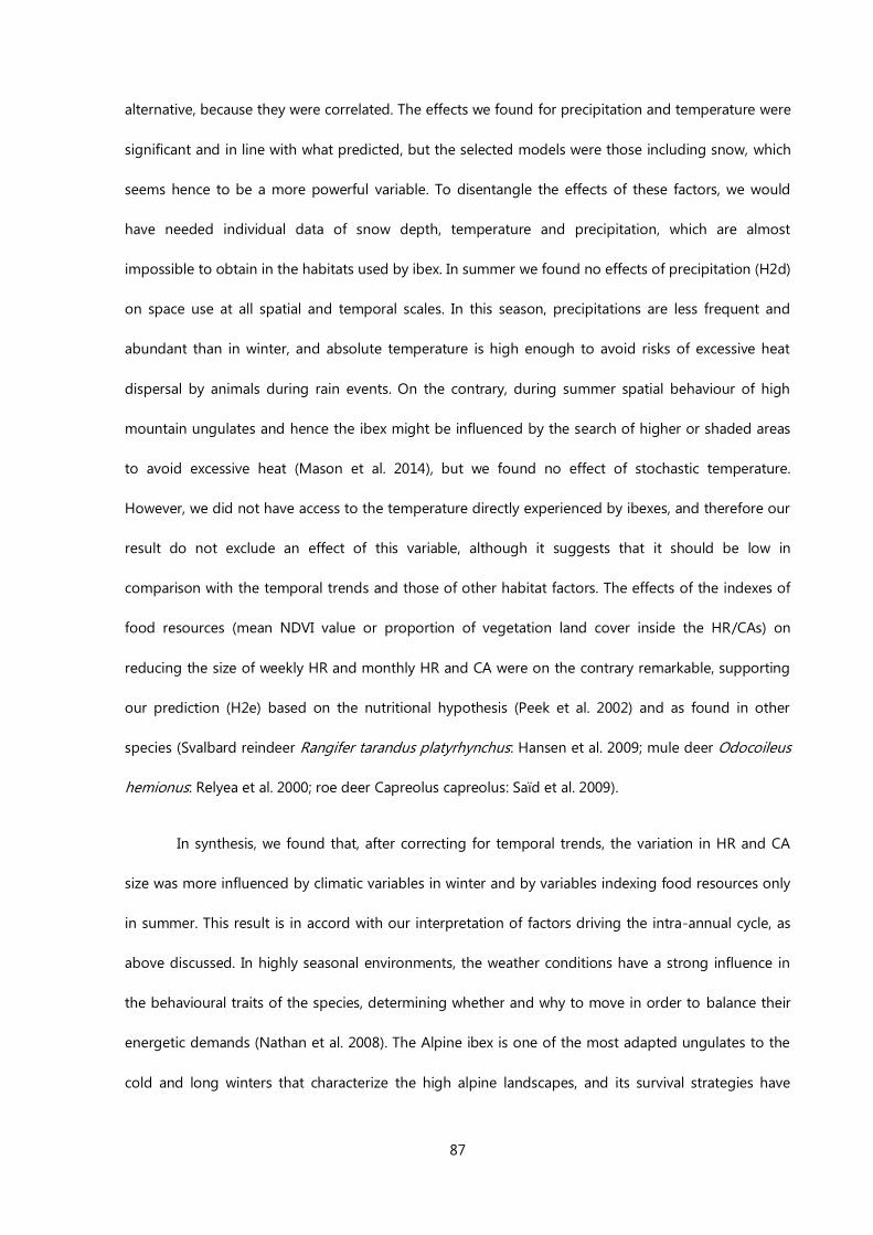
87
alternative, because they were correlated. The effects we found for precipitation and temperature were
significant and in line with what predicted, but the selected models were those including snow, which
seems hence to be a more powerful variable. To disentangle the effects of these factors, we would
have needed individual data of snow depth, temperature and precipitation, which are almost
impossible to obtain in the habitats used by ibex. In summer we found no effects of precipitation (H2d)
on space use at all spatial and temporal scales. In this season, precipitations are less frequent and
abundant than in winter, and absolute temperature is high enough to avoid risks of excessive heat
dispersal by animals during rain events. On the contrary, during summer spatial behaviour of high
mountain ungulates and hence the ibex might be influenced by the search of higher or shaded areas
to avoid excessive heat (Mason et al. 2014), but we found no effect of stochastic temperature.
However, we did not have access to the temperature directly experienced by ibexes, and therefore our
result do not exclude an effect of this variable, although it suggests that it should be low in
comparison with the temporal trends and those of other habitat factors. The effects of the indexes of
food resources (mean NDVI value or proportion of vegetation land cover inside the HR/CAs) on
reducing the size of weekly HR and monthly HR and CA were on the contrary remarkable, supporting
our prediction (H2e) based on the nutritional hypothesis (Peek et al. 2002) and as found in other
species (Svalbard reindeer Rangifer tarandus platyrhynchus: Hansen et al. 2009; mule deer Odocoileus
hemionus: Relyea et al. 2000; roe deer Capreolus capreolus: Saïd et al. 2009).
In synthesis, we found that, after correcting for temporal trends, the variation in HR and CA
size was more influenced by climatic variables in winter and by variables indexing food resources only
in summer. This result is in accord with our interpretation of factors driving the intra-annual cycle, as
above discussed. In highly seasonal environments, the weather conditions have a strong influence in
the behavioural traits of the species, determining whether and why to move in order to balance their
energetic demands (Nathan et al. 2008). The Alpine ibex is one of the most adapted ungulates to the
cold and long winters that characterize the high alpine landscapes, and its survival strategies have

88
been approached in several studies (Aublet et al. 2009; Signer et al. 2011). Our findings confirm that
climate parameters may have a strong effect on the spatial behaviour of large herbivores (Börger et al.
2006, Aublet et al. 2009, Bourgoin et al. 2011, van Beest et al. 2012), especially at fine spatio-temporal
scales (Loe et al. 2007, van Beest et al. 2011).
Habitats used by Alpine ibex are characterized by rugged terrains and steep slopes, that make
the ibex one of the ungulates with greater skill and agility to move in rocky environments (Geist 1987,
Tosi and Pedrotti 2003). The selection of steep habitat features has been attributed to several reasons
in mountain species, from refuge to warmth or human disturbance (Dussault et al. 2005, Zweifel-
Schielly et al. 2009), to exploitation of snow-free patches during winter (Rideout and Hoffman 1975,
Gross et al. 2002), or to protection of offspring during the weaning period, a widespread behaviour
among ungulates (Festa-Bianchet 1988, Boschi and Nievergelt 2003, Grignolio et al. 2007). Our results
confirm our prediction (H3): as expected, we observed that females reduced the size of the areas used
with increasing slope, at all spatial and temporal scales both in summer and winter seasons, except
only for the CA during winter. On the other hand, CAs in winter were very small, and ibexes appeared
to use also forest areas, where slope is less important as shelter habitats (see Supplementary material).
Our results are consistent with the spatial behaviour of males within the same population, described by
Scillitani et al. (2012).
We found significant but contrasting effects of the age class on space use, with subadult
females having smaller HR sizes than adults at the weekly scale in summer, but larger CA sizes at the
monthly scale in winter. The result for summer is in contrast with our expectations (H4a) and with the
results reported for the resident ibex population in the Gran Paradiso National Park (Grignolio et al.
2004). Dominance or social interactions between females (Hamel and Côté 2007), that are still
unexplored for the Alpine ibex, might perhaps explain this difference with the colony in the Gran
Paradiso National, characterized by higher population densities (Jacobson et al. 2004). However, our

89
findings were due to very few individuals in the subadult age class, and we think that they should be
taken with great caution.
Reproductive status had no effects on space use, in contrast with our expectation (H4b). In this
case, the lack of effects was very clear and consistent across spatial and temporal scales, and the
lactating and non-lactating classes were equilibrated in number of individuals/seasons. Females with
kids might increase their ranges in response to anti-predatory behaviour (White and Berger 2001) and
higher costs of lactation (Parker et al. 1990, Robbins 1993, Zimmerman et al. 2006, Main 2008). Such
response during the stages of pregnancy and weaning has been reported in ibex (Grignolio et al. 2003,
2005) and other mountain species (Iberian ibex Capra pyrenaica: Escòs and Alados, 1992; Alpine
chamois Rupicapra rupicapra: Boschi and Nievergelt 2003). In support to our result, we may consider
that females ibex have a gregarious behaviour (Gross et al. 1995), as other Caprinae species (Asiatic
ibex Capra ibex sibirica: Fox et al. 1992; Iberian ibex: Granados et al. 2001), whith groups composed by
both barren and lactating females. Lactating females might compensate the higher costs by dedicating
more time to grazing (Neuhaus and Ruckstuhl 2002), or even increasing digestive efficiency
(Zimmerman et al. 2006, Monteith et al. 2014). In any case, although we believe that the effects of
individual status should be further investigated with a larger individual sample, our results support the
prediction (H4c) that such effects are in female ibexes much less pronounced than in females of other,
non-gregarious species.


91
Table 1. Solutions of the fixed effects retained by the most parsimonious linear mixed models in summer and
winter at a weekly scale.
Table 2. Solutions of the fixed effects retained by most parsimonious linear mixed models in summer and winter
seasons at a monthly scale
HR CA
Summer l.s.
estimate SE DF t P
l.s.
estimate SE DF t P
Intercept 4.174 0.111 48 37.57 <0.001 2.076 0.114 48 18.234 <0.001
Daylight 0.312 0.093 48 3.36 <0.01 0.239 0.106 48 2.25 <0.05
Vegetation vs
Scree-rocks -0.841 0.373 48 -2.25 <0.05 -1.195 0.339 48 -3.528 <0.001
Slope -0.385 0.097 48 <0.001 <0.01 -0.368 0.0768 48 -4.80 <0.001
Winter
Intercept 3.400 0.090 79 37.75 <0.001 0.894 0.134 79 6.673 <0.001
Subadult vs
Adult -- -- -- -- -- 0.610 0.248 79 2.455 <0.05
Temperature
(absolute) 0.153 0.174 79 8.758 <0.001 0.251 0.018 79 13.88 <0.001
Slope -0.321 0.074 79 -4.349 <0.001 -- -- -- -- --
Snow
(stochastic) -0.189 0.067 79 -2.842 <0.01 -- -- -- -- --
Precipitations
(stochastic) -- -- -- -- -- -0.247 0.079 79 -3.132 <0.01
HR CA
Summer l.s.
estimate SE DF t P
l.s.
estimate SE DF t P
Intercept 3.429 0.237 214 14.482 <0.001 0.850 0.104 218 8.164 <0.001
Subadult vs
Adult -1.602 0.372 214 -4.311 <0.001 -- -- -- -- --
Daylight 0.275 0.068 214 4.047 <0.001 0.310 0.077 218 4.007 <0.001
NDVI Study
area 0.273 0.078 214 3.513 <0.001 0.561 0.079 218 7.148 <0.001
NDVI polygon -0.316 0.090 214 -3.514 <0.001 -- -- -- -- --
Slope -0.432 0.082 214 -5.250 <0.001 -0.267 0.080 218 -
3.307 <0.01
Winter
Intercept 1.612 0.085 423 18.95 <0.001 -1.213 0.103 429 -
11.77 <0.001
Daylight 0.485 0.051 423 9.56 <0.001 0.459 0.050 429 9.18 <0.001
Temperature -- -- -- -- -- 0.530 0.053 429 10.03 <0.001
Slope -0.336 0.065 423 -5.18 <0.001 -- -- -- -- --
Snow
(stochastic) -0.372 0.054 423 -6.93 <0.001 -0.406 0.058 429 -7.03 <0.001

92
Figure 1: smoothing splines of week and month on weekly and monthly HR and CA.
Figure 2: smoothing spline of week on daylight, NDVI of study area, and temperature (absolute)

93
Appendix table I: correlations between covariate variables in summer at a weekly temporal scale.
Daylig
ht
Tem
pera
ture
(ab
solu
te)
Tem
pera
ture
(sto
chast
ic)
Pre
cip
itati
on
(sto
chast
ic)
Slo
pe
ND
VI
Stu
dy a
rea
ND
VI
po
lyg
on
Daylight
-0.056 -0.011 -0.013 0.097 -0.160 -0.165
Temperature (absolute)
0.682 -0.093 -0.100 0.620 0.170
Temperature (stochastic)
-0.165 0.061 0.182 0.023
Precipitation (stochastic)
-0.019 0.170 0.183
Slope
-0.212 -0.047
NDVI Study area
0.407
Appendix table II: correlations between covariate variables in winter at a weekly temporal scale
Daylig
ht
Tem
pera
ture
(ab
slo
ute
)
Slo
pe
Sn
ow
dep
th
(sto
chast
ic)
Tem
pera
rtu
re
(sto
chast
ic)
Pre
cip
itati
on
(Sto
chast
ic)
ND
VI
Stu
dy a
rea
Daylight
0.054 -0.166 -0.028 -0.025 0.007 0.473
Temperature (absolute)
0.023 -0.171 -0.029 0.074 -0.005
Slope
0.085 0.021 0.060 -0.307
Snow (stochastic)
-0.460 0.455 -0.308
Temperature (stochastic)
-0.322 0.177
Precipitation (stochastic)
-0.066
Appendix table III: correlations between covariate variables in summer at a monthly temporal scale.
Daylig
ht
Tem
pera
ture
ND
VI
stu
dy a
rea
Tem
pre
ratu
re
(sto
chast
ic)
Pre
cip
itato
n
(sto
chast
ic)
Slo
pe
Daylight
0.014 -0.327 -0.010 -0.001 -0.081
Temperature (absolute)
0.801 0.603 -0.054 -0.110
NDVI study area
0.319 0.065 -0.048
NDVI polygon 0.234 0.196 -0.273
Temperature (stochastic)
-0.153 0.029
Precipitation (stochastic)
-0.002
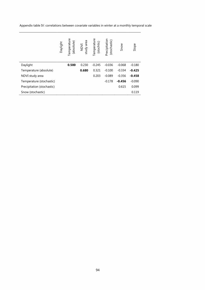
94
Appendix table IV: correlations between covariate variables in winter at a monthly temporal scale
D
aylig
ht
Tem
pera
ture
(ab
solu
te)
ND
VI
stu
dy a
rea
Tem
pera
ture
(sto
chti
c)
Pre
cip
itati
on
(sto
chast
ic)
Sn
ow
Slo
pe
Daylight
0.500 0.230 -0.245 -0.036 -0.068 -0.180
Temperature (absolute)
0.680 0.321 -0.100 -0.334 -0.425
NDVI study area
0.203 -0.089 -0.356 -0.458
Temperature (stochastic)
-0.178 -0.456 -0.090
Precipitation (stochastic)
0.615 0.099
Snow (stochastic)
0.119

95
Appendix table V: model selection for summer weekly HR and CA
Kid
Ag
e C
lass
Daylig
ht
ab
solu
te
ND
VI
Stu
dy a
rea
Tem
pera
ture
ab
solu
te
Pre
vale
nt
Lan
d
Co
ver
ND
VI H
R
slo
pe
Tem
pera
ture
sto
chast
ic
Pre
cip
itati
on
sto
chast
ic
AIC
Δ A
IC
Ho
me r
an
ge
1 X X X X -- X X X X X 725.21 14.54
2 X X X -- X X X X -- X 726.51 15.84
3 X X X X -- X X X -- X 720.07 9.4
4 -- X X X -- X X X -- -- 713.19 2.52
5 -- X X X -- X X -- -- 710.67 0
6 -- -- X X -- X X -- -- 720.86 10.19
7 -- -- X X -- X -- -- -- 735.34 24.67
8 -- -- X X -- -- -- -- -- 746.74 36.07
9 -- -- X -- -- -- -- -- -- 750.93 40.26
Null 759.77 49.1
Co
re a
rea
1 X X X X -- X X X X X 783.56 18.65
2 X X X -- X X X X -- X 792.67 27.76
3 X X X X -- X X X -- X 779.31 14.4
4 X X X X -- X -- X -- X 774.58 9.67
5 X -- X X -- X -- X -- X 771.94 7.03
6 X -- X X -- -- X -- X 768.90 3.99
7 -- -- X X -- -- -- X -- X 766.16 1.25
8 -- -- X X -- -- X -- -- 764.91 0
9 -- -- X X -- -- -- -- -- 770.37 5.46
10 -- -- X -- -- -- -- -- -- 816.59 46.22
Null -- -- X -- -- -- -- -- -- 818.05 53.14

96
Appendix table VI: model selection for winter weekly HR and CA
Ag
cla
ss
Pre
vale
nt
Lan
d
Co
ver
Daylig
ht
ab
solu
te
Tem
pera
ture
ab
sollu
te
ND
VI
Stu
dy a
rea
slo
pe
Sn
ow
sto
ch
ast
ic
Tem
pera
ture
sto
chast
ic
Pre
cip
itati
on
sto
chast
ic
AIC
Δ A
IC
Ho
me r
an
ge
1 X X X X -- X X -- -- 1331.71 5.03
2 X X -- X X X X X -- 1368.03 41.35
3 X -- X X -- X X -- -- 1329.84 3.16
4 -- -- X -- -- X X -- -- 1330.76 4.08
5 -- -- X -- -- X X -- -- 1326.68 0
6 -- -- X -- -- X -- X -- 1368.33 41.65
7 -- -- X -- -- X -- -- X 1370.16 43.48
8 -- -- X -- -- X -- -- -- 1366.30 39.62
9 -- -- X -- -- -- -- -- -- 1391.46 64.78
Null -- -- -- -- -- -- -- -- 1476.69 150.01
Co
re a
rea
1 X X X X -- X X -- -- 1263.11 6.24
2 X X -- X X X X -- -- 1281.45 24.58
3 X -- X X -- X X -- -- 1259.82 2.95
4 -- -- X X -- X X -- -- 1259.21 2.34
5 -- -- X X -- -- X -- -- 1256.87 0
6 -- -- X X -- -- -- X -- 1271.12 14.25
7 -- -- X X -- -- -- -- X 1301.22 44.35
8 -- -- X X -- -- -- -- -- 1297.96 41.09
9 -- -- X -- -- -- -- -- -- 1416.84 159.97
Null -- -- -- -- -- -- -- -- -- 1557.18 300.31

97
Appendix table VII: model selection for monthly HR and CA in summer
KId
Ag
e C
lass
Daylig
ht
Pre
vale
nt
lan
d
co
ver
Slo
pe
Ab
solu
te
tem
pera
ture
ND
VI st
ud
y a
rea
ND
VI p
oly
go
n
Tem
pera
ture
sto
chast
ic
Pre
cip
itati
on
sto
chast
ic
AIC
Δ A
IC
Ho
me r
an
ges
1 X X X X X X -- -- -- X 121.97 12.23
2 X X X X X -- X -- -- X 121.53 11.79
3 X X X X X -- -- X -- X 121.27 11.53
4 X X X X X -- -- -- X X 123.68 13.94
5 -- X X X X X -- -- -- X 117.91 8.17
6 -- -- X X X X -- -- -- X 115.54 5.8
7 -- -- X X X X -- -- -- -- 112.94 3.2
8 -- -- X X X -- X -- -- -- 112.86 3.12
9 -- -- X X X -- -- X -- -- 112.79 3.05
10 -- -- X X X -- -- -- -- -- 109.74 0
11 -- -- X X -- -- -- -- -- -- 118.33 8.59
12 -- -- X -- -- -- -- -- -- -- 121.98 12.24
Null -- -- -- -- -- -- -- -- -- -- 129.36 19.62
Co
re a
reas
1 X X X X X X -- -- -- X 141.64 14.84
2 X X X X X -- X -- -- X 139.19 12.39
3 X X X X X -- -- X -- X 140.66 13.86
4 X X X X X -- -- -- X X 143.84 17.04
5 -- X X X X -- X -- -- X 135.22 8.42
6 -- -- X X X -- X -- -- X 131.59 4.79
7 -- -- X X X -- X -- -- -- 126.95 -0.15
10 -- -- X X X -- -- -- -- -- 126.80 0
11 -- -- X X -- -- -- -- -- -- 141.29 14.49
12 -- -- X -- -- -- -- -- -- -- 145.61 18.81
Null -- -- -- -- -- -- -- -- -- -- 146.28 19.48
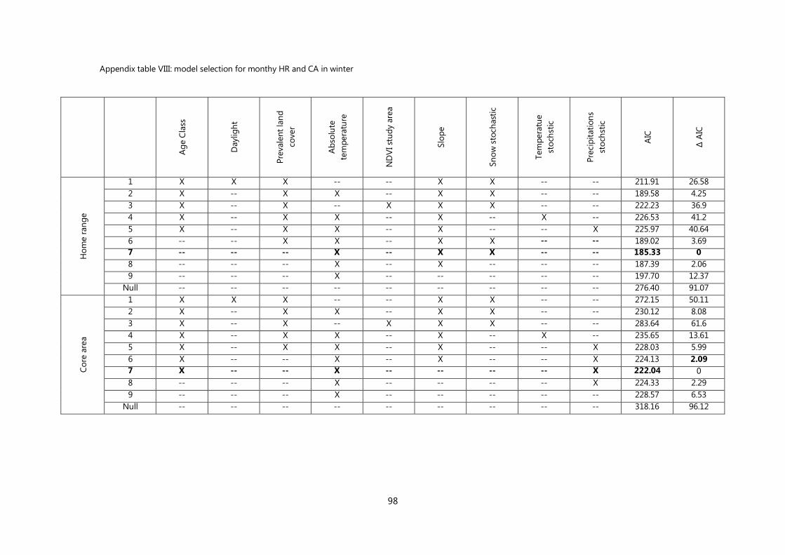
98
Appendix table VIII: model selection for monthy HR and CA in winter
Ag
e C
lass
Daylig
ht
Pre
vale
nt
lan
d
co
ver
Ab
solu
te
tem
pera
ture
ND
VI st
ud
y a
rea
Slo
pe
Sn
ow
sto
ch
ast
ic
Tem
pera
tue
sto
chst
ic
Pre
cip
itati
on
s
sto
chst
ic
AIC
Δ A
IC
Ho
me r
an
ge
1 X X X -- -- X X -- -- 211.91 26.58
2 X -- X X -- X X -- -- 189.58 4.25
3 X -- X -- X X X -- -- 222.23 36.9
4 X -- X X -- X -- X -- 226.53 41.2
5 X -- X X -- X -- -- X 225.97 40.64
6 -- -- X X -- X X -- -- 189.02 3.69
7 -- -- -- X -- X X -- -- 185.33 0
8 -- -- -- X -- X -- -- -- 187.39 2.06
9 -- -- -- X -- -- -- -- -- 197.70 12.37
Null -- -- -- -- -- -- -- -- -- 276.40 91.07
Co
re a
rea
1 X X X -- -- X X -- -- 272.15 50.11
2 X -- X X -- X X -- -- 230.12 8.08
3 X -- X -- X X X -- -- 283.64 61.6
4 X -- X X -- X -- X -- 235.65 13.61
5 X -- X X -- X -- -- X 228.03 5.99
6 X -- -- X -- X -- -- X 224.13 2.09
7 X -- -- X -- -- -- -- X 222.04 0
8 -- -- -- X -- -- -- -- X 224.33 2.29
9 -- -- -- X -- -- -- -- -- 228.57 6.53
Null -- -- -- -- -- -- -- -- -- 318.16 96.12

99
Supplementary material: Identification of biological seasons
We used data from 12 females for a total of 87.795 hourly locations. We associated each
location with the corresponding elevation (m), slope (°), prevalent land use category (forest, grasslands,
scree+rocks), activity index (calculated as the average of the XY activity values from the accelerometer
embedded to the GPS collar in the 10 minutes immediately preceding and following the scheduled
time for the location), and distance (m) from the previous location (distance was calculated only
between fixes separated by 1 h).
We then calculated for each Julian date the average values of elevation, slope, activity index
and distance, and the frequency of each land use category (across individuals and years). Julian dates
were then grouped into “seasons” using a clustering procedure (proc cluster, SAS©
9.2)
Figure A1: Results from the clustering procedure to identify the experienced seasons of the female ibex in the
Marmolada Massif.

100
0
1
2
0
9
18
27
36
45
54
63
74
83
92
10
1
11
0
11
9
12
8
13
7
14
6
15
5
16
4
17
3
18
2
19
1
20
0
20
9
21
8
22
7
23
6
24
5
25
4
26
3
27
2
28
1
29
0
29
9
30
8
31
7
32
6
33
5
34
4
35
3
clu
ste
r
Julian date
The results supported the presence of two or three clusters (Figure A1). With two clusters,
Julian dates were divided into a prolonged winter of around 225 days and a short summer lasting
around 140 days (Figure A2).
Figure A2. Assignment of Julian dates (0 = December 21st) to clusters 1 (summer) or 2 (winter).
As respect to summer, winter was characterized by lower elevations, smaller use of scree and
rocks, higher use of grasslands and forest, lower activity and speed index values (Table A1). Only slope
did not differ between clusters.
Table A1. Profiles of the two clusters (mean ± SD) for the considered variables.
With three clusters, one cluster corresponded to a prolonged winter season, a second cluster
to a shorter summer season, and the third cluster to two very short periods (approximately 30-40 days)
Winter Summer
Mean SD Mean SD
Elevation (m) 2097 74 2380 68
Slope (°) 47.3 2.5 44.5 1.8
Grasslands (%) 14.3 7.0 7.7 4.3
Forest (%) 29.5 11.6 5.9 4.3
Screes + rocks (%) 55.0 10.7 85.5 7.5
Activity index 21.9 8.0 35.6 7.2
Speed index (m/h) 61.5 51.0 125.7 62.9
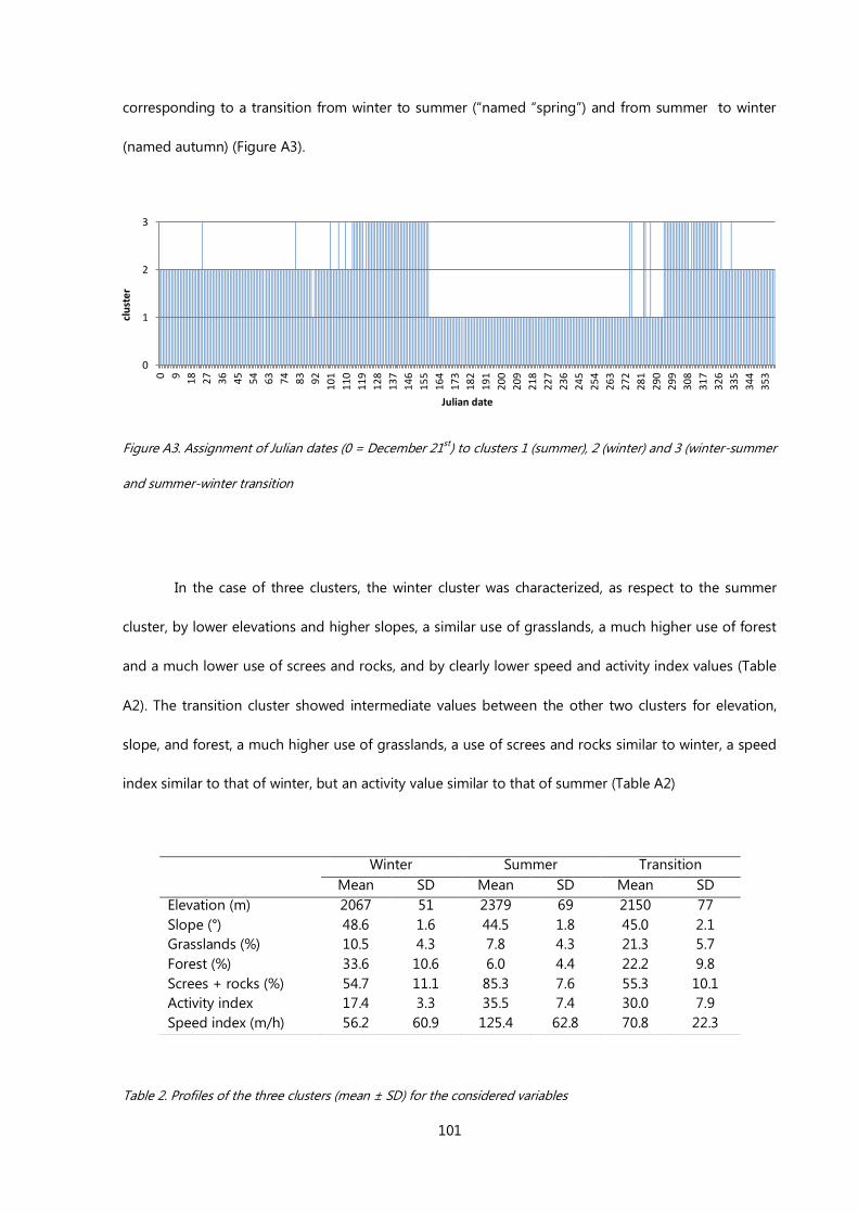
101
0
1
2
3
0
9
18
27
36
45
54
63
74
83
92
10
1
11
0
11
9
12
8
13
7
14
6
15
5
16
4
17
3
18
2
19
1
20
0
20
9
21
8
22
7
23
6
24
5
25
4
26
3
27
2
28
1
29
0
29
9
30
8
31
7
32
6
33
5
34
4
35
3
clu
ste
r
Julian date
corresponding to a transition from winter to summer (“named “spring”) and from summer to winter
(named autumn) (Figure A3).
Figure A3. Assignment of Julian dates (0 = December 21st) to clusters 1 (summer), 2 (winter) and 3 (winter-summer
and summer-winter transition
In the case of three clusters, the winter cluster was characterized, as respect to the summer
cluster, by lower elevations and higher slopes, a similar use of grasslands, a much higher use of forest
and a much lower use of screes and rocks, and by clearly lower speed and activity index values (Table
A2). The transition cluster showed intermediate values between the other two clusters for elevation,
slope, and forest, a much higher use of grasslands, a use of screes and rocks similar to winter, a speed
index similar to that of winter, but an activity value similar to that of summer (Table A2)
Table 2. Profiles of the three clusters (mean ± SD) for the considered variables
Winter Summer Transition
Mean SD Mean SD Mean SD
Elevation (m) 2067 51 2379 69 2150 77
Slope (°) 48.6 1.6 44.5 1.8 45.0 2.1
Grasslands (%) 10.5 4.3 7.8 4.3 21.3 5.7
Forest (%) 33.6 10.6 6.0 4.4 22.2 9.8
Screes + rocks (%) 54.7 11.1 85.3 7.6 55.3 10.1
Activity index 17.4 3.3 35.5 7.4 30.0 7.9
Speed index (m/h) 56.2 60.9 125.4 62.8 70.8 22.3

102
LITERATURE CITED
Albon, S. D., and Langvatn, R. (1992). Plant phenology and the benefits of migration in a temperate
ungulate. Oikos, 502-513.
Apollonio, M., Brivio, F., Rossi, I., Bassano, B., and Grignolio, S. (2013). Consequences of snowy winters
on male mating strategies and reproduction in a mountain ungulate. Behavioural processes, 98, 44-50.
Aublet, J. F., Festa-Bianchet, M., Bergero, D., and Bassano, B. (2009). Temperature constraints on
foraging behaviour of male Alpine ibex (Capra ibex) in summer. Oecologia, 159(1), 237-247.
Benhamou, S., and Riotte-Lambert, L. (2012). Beyond the Utilization Distribution: Identifying home
range areas that are intensively exploited or repeatedly visited. Ecological Modelling, 227, 112-116.
Bjørneraas, K., MOORTER, B., Rolandsen, C. M., and Herfindal, I. (2010). Screening global positioning
system location data for errors using animal movement characteristics. The Journal of Wildlife
Management, 74(6), 1361-1366.
Börger, L., Franconi, N., De Michele, G., Gantz, A., Meschi, F., Manica, A., Lovari. S and Coulson, T. I. M.
(2006a). Effects of sampling regime on the mean and variance of home range size estimates. Journal of
Animal Ecology, 75(6), 1393-1405.
Börger, L., Franconi, N., Ferretti, F., Meschi, F., De Michele, G., Gantz, A., and Coulson, T. (2006b). An
integrated approach to identify spatiotemporal and individual‐level determinants of animal home
range size. The American Naturalist, 168(4), 471-485.
Börger, L., Dalziel, B. D., and Fryxell, J. M. (2008). Are there general mechanisms of animal home range
behaviour? A review and prospects for future research. Ecology letters, 11(6), 637-650.
Boschi, C., and Nievergelt, B. (2003). The spatial patterns of Alpine chamois (Rupicapra rupicapra
rupicapra) and their influence on population dynamics in the Swiss National Park. Mammalian Biology-
Zeitschrift für Säugetierkunde, 68(1), 16-30.
Bourgoin, G., Garel, M., Blanchard, P., Dubray, D., Maillard, D., and Gaillard, J. M. (2011). Daily responses
of mouflon (Ovis gmelini musimon× Ovis sp.) activity to summer climatic conditions. Canadian Journal
of Zoology, 89(9), 765-773.
Bowyer, R. T. (1984). Sexual segregation in southern mule deer. Journal of Mammalogy, 410-417.
Bremset Hansen, B., Herfindal, I., Aanes, R., Sæther, B. E., and Henriksen, S. (2009). Functional response
in habitat selection and the tradeoffs between foraging niche components in a large herbivore. Oikos,
118(6), 859-872.
Brivio, F., Grignolio, S., Brambilla, A., and Apollonio, M. (2014). Intra-sexual variability in feeding
behaviour of a mountain ungulate: size matters. Behavioral Ecology and Sociobiology, 68(10), 1649-
1660.
Burt, W. H. (1943). Territoriality and home range concepts as applied to mammals. Journal of
mammalogy, 24(3), 346-352.

103
Calenge, C. (2006). The package “adehabitat” for the R software: a tool for the analysis of space and
habitat use by animals. Ecological modelling, 197(3), 516-519.
Caswell, L. R., and Savannunt, D. S. (1988). Temperature and solvent effects on the experimental dipole
moments of three crown ethers. Journal of heterocyclic chemistry, 25(1), 73-79.
Cederlund, G., and Sand, H. (1994). Home-range size in relation to age and sex in moose. Journal of
Mammalogy, 1005-1012.
Corlatti, L., Bassano, B., Valencak, T. G., and Lovari, S. (2013a). Foraging strategies associated with
alternative reproductive tactics in a large mammal. Journal of Zoology, 291(2), 111-118.
Corlatti, L., Caroli, M., Pietrocini, V., and Lovari, S. (2013b). Rutting behaviour of territorial and
nonterritorial male chamois: Is there a home advantage?. Behavioural processes, 92, 118-124.
Côté, S. D., and Festa-Bianchet, M. (2003). Mountain goat. Montana, 2, 3-045.
Creel, S., Fox, J. E., Hardy, A., Sands, J., Garrott, B., and Peterson, R. O. (2002). Snowmobile activity and
glucocorticoid stress responses in wolves and elk. Conservation Biology, 16(3), 809-814.
Dahle, B., and Swenson, J. E. (2003). Home ranges in adult Scandinavian brown bears (Ursus arctos):
effect of mass, sex, reproductive category, population density and habitat type. Journal of Zoology,
260(4), 329-335.
Dalziel, B. D., Morales, J. M., and Fryxell, J. M. (2008). Fitting probability distributions to animal
movement trajectories: using artificial neural networks to link distance, resources, and memory. The
American Naturalist, 172(2), 248-258.
Danilkin, A. A., and Hewison, A. M. (1996). Behavioural ecology of Siberian and European roe deer.
D'Eon, R. G., and Serrouya, R. (2005). Mule deer seasonal movements and multiscale resource selection
using global positioning system radiotelemetry. Journal of Mammalogy, 86(4), 736-744.
Dussault, C., Courtois, R., Ouellet, J. P., and Girard, I. (2005). Space use of moose in relation to food
availability. Canadian journal of zoology, 83(11), 1431-1437.
Escos, J., and Alados, C. L. (1992). The home-range of the Spanish ibex in spring and fall. Mammalia,
56(1), 57-64.
Ferretti, F., Costa, A., Corazza, M., Pietrocini, V., Cesaretti, G., and Lovari, S. (2014). Males are faster
foragers than females: intersexual differences of foraging behaviour in the Apennine chamois.
Behavioral ecology and sociobiology, 68(8), 1335-1344.
Festa-Bianchet, M. (1988). Seasonal range selection in bighorn sheep: conflicts between forage quality,
forage quantity, and predator avoidance.Oecologia, 75(4), 580-586.
Fieberg, J., Matthiopoulos, J., Hebblewhite, M., Boyce, M. S., and Frair, J. L. (2010). Correlation and
studies of habitat selection: problem, red herring or opportunity?. Philosophical Transactions of the
Royal Society B: Biological Sciences, 365(1550), 2233-2244.

104
Fox, J. L., Sinha, S. P., and Chundawat, R. S. (1992). Activity patterns and habitat use of ibex in the
Himalaya mountains of India. Journal of Mammalogy, 527-534.
Gaillard, J. M., Hebblewhite, M., Loison, A., Fuller, M., Powell, R., Basille, M., and Van Moorter, B. (2010).
Habitat–performance relationships: finding the right metric at a given spatial scale.
Geist, V. (1987). On the evolution of the Caprinae. In The biology and management of Capricornis and
related mountain Antelopes (pp. 3-40). Springer Netherlands.
Getz, W. M., and Wilmers, C. C. (2004). A local nearest‐neighbor convex‐hull construction of home
ranges and utilization distributions. Ecography, 27(4), 489-505.
Getz, W. M., Fortmann-Roe, S., Cross, P. C., Lyons, A. J., Ryan, S. J., and Wilmers, C. C. (2007). LoCoH:
nonparameteric kernel methods for constructing home ranges and utilization distributions. PloS one,
2(2), e207.
Granados, J. E., Pérez, J. M., Márquez, F. J., Serrano, E., Soriguer, R. C., and Fandos, P. (2001). La cabra
montés (Capra pyrenaica, Schinz 1838). Galemys, 13(1), 3-37.
Grignolio, S., Parrini, F., Bassano, B., Luccarini, S., and Apollonio, M. (2003). Habitat selection in adult
males of Alpine ibex, Capra ibex ibex. Folia Zoologica, 52(2), 113-120.
Grignolio, S., Rossi, I., Bassano, B., Parrini, F., and Apollonio, M. (2004). Seasonal variations of spatial
behaviour in female Alpine ibex (Capra ibex ibex) in relation to climatic conditions and age. Ethology
Ecology and Evolution, 16(3), 255-264.
Grignolio, S., Rossi, I., Bertolotto, E., Bassano, B., and Apollonio, M. (2007). Influence of the kid on space
use and habitat selection of female Alpine ibex. The Journal of wildlife management, 71(3), 713-719.
Green, W. C. (1992). Social influences on contact maintenance interactions of bison mothers and
calves: group size and nearest-neighbour distance. Animal behaviour, 43(5), 775-785.
Gross, J. E., Kneeland, M. C., Reed, D. F., and Reich, R. M. (2002). GIS-based habitat models for
mountain goats. Journal of Mammalogy, 83(1), 218-228.
Gross†‡, . E., Alkon‡, P. U., and Demment†, M. W. (1995). Grouping patterns and spatial segregation by
Nubian ibex. Journal of Arid Environments, 30(4), 423-439
GRØTAN, V., SÆTHER, B. E., Filli, F., and Engen, S. (2008). Effects of climate on population fluctuations
of ibex. Global Change Biology, 14(2), 218-228.
Hamel, S., and Côté, S. D. (2007). Habitat use patterns in relation to escape terrain: are alpine ungulate
females trading off better foraging sites for safety?. Canadian Journal of Zoology, 85(9), 933-943.
Hamel, S., Garel, M., Festa‐Bianchet, M., Gaillard, J. M., and Côté, S. D. (2009). Spring Normalized
Difference Vegetation Index (NDVI) predicts annual variation in timing of peak faecal crude protein in
mountain ungulates. Journal of Applied Ecology, 46(3), 582-589.
Hansen, B. B., Aanes, R., Herfindal, I., Sæther, B. E., and Henriksen, S. (2009). Winter habitat–space use in
a large arctic herbivore facing contrasting forage abundance. Polar biology, 32(7), 971-984.

105
Harestad, A. S., and Bunnel, F. L. (1979). Home range and body weight--a reevaluation. Ecology, 389-
402.
Hamr, J. (1988). Disturbance behaviour of chamois in an alpine tourist area of Austria. Mountain
Research and Development, 65-73.
Huete, A., Didan, K., Miura, T., Rodriguez, E. P., Gao, X., and Ferreira, L. G. (2002). Overview of the
radiometric and biophysical performance of the MODIS vegetation indices. Remote sensing of
environment, 83(1), 195-213.
Illius, A. W., and Gordon, I. J. (1987). The allometry of food intake in grazing ruminants. The Journal of
Animal Ecology, 989-999.
Illius, A. W., and Gordon, I. J. (1992). Modelling the nutritional ecology of ungulate herbivores:
evolution of body size and competitive interactions. Oecologia, 89(3), 428-434.
Jacobson, A. R., Provenzale, A., von Hardenberg, A., Bassano, B., and Festa-Bianchet, M. (2004). Climate
forcing and density dependence in a mountain ungulate population. Ecology, 85(6), 1598-1610.
Johnson, A. R., Wiens, J. A., Milne, B. T., and Crist, T. O. (1992). Animal movements and population
dynamics in heterogeneous landscapes. Landscape ecology, 7(1), 63-75.
Kaufman, L., and Rousseeuw, P. J. (2009). Finding groups in data: an introduction to cluster analysis
(Vol. 344). John Wiley and Sons.
Kie, J. G., Matthiopoulos, J., Fieberg, J., Powell, R. A., Cagnacci, F., Mitchell, M. S., ... and Moorcroft, P. R.
(2010). The home-range concept: are traditional estimators still relevant with modern telemetry
technology?. Philosophical Transactions of the Royal Society B: Biological Sciences, 365(1550), 2221-
2231.
Kjellander, P., Hewison, A. J. M., Liberg, O., Angibault, J. M., Bideau, E., and Cargnelutti, B. (2004).
Experimental evidence for density-dependence of home-range size in roe deer (Capreolus capreolus
L.): a comparison of two long-term studies. Oecologia, 139(3), 478-485.
Loe, L. E., Mysterud, A., Stien, A., Steen, H., Evans, D. M., and Austrheim, G. (2007). Positive short-term
effects of sheep grazing on the alpine avifauna.Biology Letters, 3(1), 110-112.
Main, M. B. (2008). Reconciling competing ecological explanations for sexual segregation in
ungulates. Ecology, 89(3), 693-704.
Manor, R., and Saltz, D. (2003). Impact of human nuisance disturbance on vigilance and group size of a
social ungulate. Ecological Applications, 13(6), 1830-1834.
Mason, T. H., Stephens, P. A., Apollonio, M., and Willis, S. G. (2014). Predicting potential responses to
future climate in an alpine ungulate: interspecific interactions exceed climate effects. Global change
biology, 20(12), 3872-3882.
McNab, B. K. (1963). Bioenergetics and the determination of home range size. American Naturalist,
133-140.
106
Monteith, K. B., Monteith, K. L., Bowyer, R. T., Leslie Jr, D. M., and Jenks, J. A. (2014). Reproductive
effects on fecal nitrogen as an index of diet quality: an experimental assessment. Journal of
Mammalogy, 95(2), 301-310
Moorcroft, P. R. (2012). Mechanistic approaches to understanding and predicting mammalian space
use: recent advances, future directions. Journal of Mammalogy, 93(4), 903-916.
Morales, J. M., Haydon, D. T., Frair, J., Holsinger, K. E., and Fryxell, J. M. (2004). Extracting more out of
relocation data: building movement models as mixtures of random walks. Ecology, 85(9), 2436-2445.
Morales, J. M., Moorcroft, P. R., Matthiopoulos, J., Frair, J. L., Kie, J. G., Powell, R. A., ... and Haydon, D. T.
(2010). Building the bridge between animal movement and population dynamics. Philosophical
Transactions of the Royal Society B: Biological Sciences, 365(1550), 2289-2301.
Morellet, N., Bonenfant, C., Börger, L., Ossi, F., Cagnacci, F., Heurich, M., ... and Mysterud, A. (2013).
Seasonality, weather and climate affect home range size in roe deer across a wide latitudinal gradient
within Europe. Journal of Animal Ecology, 82(6), 1326-1339.
Mueller, T., Olson, K. A., Dressler, G., Leimgruber, P., Fuller, T. K., Nicolson, C., ... and Fagan, W. F. (2011).
How landscape dynamics link individual‐to population‐level movement patterns: a multispecies
comparison of ungulate relocation data. Global Ecology and Biogeography, 20(5), 683-694.
Nathan, R., Getz, W. M., Revilla, E., Holyoak, M., Kadmon, R., Saltz, D., and Smouse, P. E. (2008). A
movement ecology paradigm for unifying organismal movement research. Proceedings of the National
Academy of Sciences, 105(49), 19052-19059.
Neuhaus, P., and Ruckstuhl, K. E. (2002). Foraging behaviour in Alpine ibex (Capra ibex): consequences
of reproductive status, body size, age and sex.Ethology Ecology and Evolution, 14(4), 373-381.
Nilsen, E. B., Linnell, J. D., and Andersen, R. (2004). Individual access to preferred habitat affects fitness
components in female roe deer Capreolus capreolus. Journal of Animal Ecology, 73(1), 44-50.
Owen-Smith, N., Fryxell, J. M., and Merrill, E. H. (2010). Foraging theory upscaled: the behavioural
ecology of herbivore movement. Philosophical Transactions of the Royal Society B: Biological Sciences,
365(1550), 2267-2278.
Parrini, F., Grignolio, S., Luccarini, S., Bassano, B., and Apollonio, M. (2003). Spatial behaviour of adult
male Alpine ibex Capra ibex ibex in the Gran Paradiso National Park, Italy. Acta Theriologica, 48(3),
411-423.
Peek, J. M., Dennis, B., and Hershey, T. (2002). Predicting population trends of mule deer. The Journal of
wildlife management, 729-736.
Pettorelli, N., Pelletier, F., Hardenberg, A. V., Festa-Bianchet, M., and Côté, S. D. (2007). Early onset of
vegetation growth vs. rapid green-up: impacts on juvenile mountain ungulates. Ecology, 88(2), 381-
390.
Pinheiro, J., Bates, D., DebRoy, S., and Sarkar, D. (2011). R Development Core Team. 2010. nlme: linear
and nonlinear mixed effects models. R package version 3.1-97. R Foundation for Statistical Computing,
Vienna.
107
Potts, J. R., and Lewis, M. A. (2014). How do animal territories form and change? Lessons from 20 years
of mechanistic modelling. Proceedings of the Royal Society B: Biological Sciences, 281(1784),
20140231.
Powell, R. A. (2000). Animal home ranges and territories and home range estimators. Research
techniques in animal ecology: controversies and consequences, 65-110.
Powell, R. A., and Mitchell, M. S. (2012). What is a home range?. Journal of Mammalogy, 93(4), 948-958.
R Development Core Team. (2008). R: A Language and Environment for Statistical Computing, version
2.7. 0. R Foundation for Statistical Computing, Vienna.
Relyea, R. A. (2000). Trait-mediated indirect effects in larval anurans: reversing competition with the
threat of predation. Ecology, 81(8), 2278-2289.
Rideout, C. B., and Hoffmann, R. S. (1975). Oreamnos americanus. Mammalian Species, 1-6.
Rivrud, I. M., Loe, L. E., and Mysterud, A. (2010). How does local weather predict red deer home range
size at different temporal scales?. Journal of Animal Ecology, 79(6), 1280-1295.
Rossi, I., Lamberti, P., Mauri, L., and Apollonio, M. (2003). Home range dynamics of male roe deer
Capreolus capreolus in a mountainous habitat. Acta theriologica, 48(3), 425-432.
Ruckstuhl, K. E., Festa-Bianchet, M., and Jorgenson, J. T. (2003). Bite rates in Rocky Mountain bighorn
sheep (Ovis canadensis): effects of season, age, sex and reproductive status. Behavioral Ecology and
Sociobiology, 54(2), 167-173.
Rughetti, M., and Festa‐Bianchet, M. (2011). Seasonal changes in sexual size dimorphism in northern
chamois. Journal of Zoology, 284(4), 257-264.
Rughetti, M., Toïgo, C., Von Hardenberg, A., Rocchia, E., and Festa-Bianchet, M. (2011). Effects of an
exceptionally snowy winter on chamois survival. Acta Theriologica, 56(4), 329-333.
Saïd, S., Gaillard, J. M., Duncan, P., Guillon, N., Guillon, N., Servanty, S., ... and Laere, G. (2005). Ecological
correlates of home-range size in spring–summer for female roe deer (Capreolus capreolus) in
Said, S., Gaillard, J. M., Widmer, O., Débias, F., Bourgoin, G., Delorme, D., and Roux, C. (2009). What
shapes intra‐specific variation in home range size? A case study of female roe deer. Oikos, 118(9),
1299-1306.
Scillitani, L., Darmon, G., Monaco, A., Cocca, G., Sturaro, E., Rossi, L., and Ramanzin, M. (2013). Habitat
selection in translocated gregarious ungulate species: an interplay between sociality and ecological
requirements. The Journal of Wildlife Management, 77(4), 761-769.
Scillitani, L., Sturaro, E., Menzano, A., Rossi, L., Viale, C., and Ramanzin, M. (2012). Post-release spatial
and social behaviour of translocated male Alpine ibexes (Capra ibex ibex) in the eastern Italian Alps.
European Journal of Wildlife Research, 58(2), 461-472.

108
Signer, C., Ruf, T., and Arnold, W. (2011). Hypometabolism and basking: the strategies of Alpine ibex to
endure harsh over‐wintering conditions. Functional Ecology, 25(3), 537-547.
Spencer, W. D. (2012). Home ranges and the value of spatial information. Journal of Mammalogy, 93(4),
929-947.
Toïgo, C., Gaillard, J. M., Festa-BianchetM., Largo, E., Michallet, J., and Maillard, D. (2007). Sex‐and
age‐specific survival of the highly dimorphic Alpine ibex: evidence for a conservative life‐history tactic.
Journal of Animal Ecology, 76(4), 679-686.
Tomkiewicz, S. M., Fuller, M. R., Kie, J. G., and Bates, K. K. (2010). Global positioning system and
associated technologies in animal behaviour and ecological research. Philosophical Transactions of the
Royal Society B: Biological Sciences, 365(1550), 2163-2176.
Tosi, G., and Pedrotti, L. (2003). Capra ibex L. Fauna d’Italia. Mammalia III Carnivora-Artiodactyla.
Calderini Edagricole, Bologna, 364-434.
Tucker, M. A., Ord, T. J., and Rogers, T. L. (2014). Evolutionary predictors of mammalian home range
size: body mass, diet and the environment. Global Ecology and Biogeography.
van Beest, F. M., Rivrud, I. M., Loe, L. E., Milner, J. M., and Mysterud, A. (2011). What determines
variation in home range size across spatiotemporal scales in a large browsing herbivore?. Journal of
Animal Ecology, 80(4), 771-785.
van Beest, F. M., Van Moorter, B., and Milner, J. M. (2012). Temperature-mediated habitat use and
selection by a heat-sensitive northern ungulate. Animal Behaviour, 84(3), 723-735.
Vincent, J. P., Bideau, E., Hewison, A. J. M., and Angibault, J. M. (1995). The influence of increasing
density on body weight, kid production, home range and winter grouping in roe deer (Capreolus
capreolus). Journal of Zoology, 236(3), 371-382.
White, K. S., Testa, J. W., and Berger, J. (2001). Behavioral and ecologic effects of differential predation
pressure on moose in Alaska. Journal of Mammalogy,82(2), 422-429.
Wood, S. N. (2001). mgcv: GAMs and generalized ridge regression for R. R news, 1(2), 20-25.
Zimmerman, T. J., Jenks, J. A., and Leslie Jr, D. M. (2006). Gastrointestinal morphology of female white-
tailed and mule deer: effects of fire, reproduction, and feeding type. Journal of Mammalogy, 87(3),
598-605.
Zuur, A. F., Ieno, E. N., Walker, N. J., Saveliev, A. A., and Smith, G. M. (2009). Limitations of linear
regression applied on ecological data. In Mixed effects models and extensions in ecology with R (pp.
11-33). Springer New York.

109
CHAPTER 3
VALIDATION OF A NON-INVASIVE TECHNIQUE FOR
ESTIMATING DIET QUALITY IN AN ALPINE UNGULATE
PARRAGA M.A., FERRAGINA A., STURARO E., BITTANTE G., RAMANZIN M.


111
INTRODUCTION
Improving the knowledge of foraging strategies of herbivore species is a fundamental basis to
understand the individual performance and reproduction success, which in turn drive the populations
dynamics (Hernandez and Laundrè 2005, Cebrian et al. 2008). Hence, spatiotemporal variation of
forage quality is an essential indicator for behavioural patterns in ungulate species living in free-
predation systems. However, developing a useful tool for determining diet quality is not a simple
matter, especially in high mountain environments where sampling plant species at a broad spatial
scale is difficult and may not reflect the real composition of animal diet.
Faecal material from wild ruminants encompasses undigested material, such as in particular
lignin, suberin, cutin and proteins, plus secondary metabolic excretions and microbial cells (Robbins
1983). Sampling faeces is possible over large temporal and spatial scales without human intervention
on animal welfare. Therefore, assessing diet quality of free-ranging animals from faecal analysis has
become a widespread technique in wildlife research (Wrench et al. 1997, Homolka and Heroldovà
2001, Showers et al. 2006, Verheyden et al. 2011). In particular, faecal nitrogen (FN) represents an
indicator of the relationship between diet properties and vegetation characteristics, due to its
correlation with plant digestibility and with dietary proteins (Holechek et al. 1982). After the ingestion
of the plants, ruminants are capable to metabolize endogenous and exogenous sources of N through
the fermentative action of anaerobic microbes located in the rumen (Van Soest 1994), and the
subsequent digestive processes lead to a proportional quantity of metabolic N excreted with the
faeces (Wehausen 1995). Higher quality and quantity of forage intakes increase fermentation rates
(Berteaux et al. 1998) and microbial activity (Hanley 1982), which ultimately turns into high levels of FN
(Schwarm et al. 2009). Although it has been demonstrated that the relation between FN and dietary N
may be affected by the presence of tannins in the plants consumed, the problem appears stronger for
browsers and mixed feeders than for grazers (Wofford et al. 1985, Robbins et al. 1987). Other faecal
constituents such as neutral detergent fibre (NDF), acid detergent fibre (ADF) or ash (AIA) are indexes

112
of low digestibility compounds normally negatively correlated with protein, and might help to predict
nutritional status of ruminants, but they seem to have a role more for integrating N results than as
single indicators (Wofford 1985).
Chemical analysis implies high labour and laboratory costs and requires samples destruction.
Therefore, other indirect methods have been developed and improved over the last years to identify
chemical compound in organic matrices. Near infrared spectroscopy (NIRS) consists in the projection
of a known quantity of NIR light onto organic substances and the recording of the reflectance or
transmittance values obtained from such substances, which depend on the characteristics and richness
of chemical bonds. Calibration equations can be obtained relating the spectral properties of a large
and diverse set of samples to the results obtained by a reference laboratory method (Stuth et al. 2003).
Then, NIRS can be used to routinely estimate chemical compounds, and has been recognized since
1970s as an optimal resource to reduce,labour, sample processing and costs inputs in the assessments
of diets in livestock using faecal samples (see Roberts et al. 2004 for a review). Lyons and Stuth (1992)
were the pioneers in the application of NIRS technology to predict diet quality in free-ranging animals.
Due to the differences on diet selectivity and digestive physiology, one faecal NIRS equation may not
be applicable from one species to another, and hence the validation of calibration models is an
essential step to predict accurate conclusions of diet quality (Leite and Stuth 1995).
Studies on several wild ungulate species also recognized that fluctuations in FN estimated
using fecal NIRS analysis follow the seasonal variation of the quality of vegetation (bighorn sheep Ovis
canadensis: Blanchard et al 2003; moose Alces alces: Leslie et al. 1989; black-tailed deer Odocoileus
hemionus columbianus: Leslie and Starkey 1985, 1987; Red deer Cervus elaphus: Kamler and Homolka
2005; roe deer Capreolus capreolus: Kamler and Homolka 2005 and Verheyden et al. 2011). To identify
the relationship between FN and plant phenology, or quality of diets, researchers have commonly used
plant samples collections or feeding trials that require remarkable effort, time and high costs
(Verheyden et al.2011, Showers et al 2006). The Normalized Difference Vegetation Index (NDVI; Tucker

113
1986) is a remotely global index of vegetation productivity measured from the red/near-infrared ratio
of growing vegetation reflectance in the electromagnetic spectrum (Jackson and Huete 1991), and
represents an attractive opportunity to monitor vegetation quality and quantity dynamics without the
need of analysing vegetation characteristics directly from field-collected samples. In addition, satellite
imagery is a proxy of vegetation dynamics across wide geographic landscapes and over a long time
scales, in this improving the opportunities of understanding the interactions between trophic resources
and behavioural patterns of free-ranging animals. Although NDVI has been used in numerous studies
across different environmental condition (see Pettorelli et al. 2005, 2011 for a review), the validation of
its biological significance in terms of plant productivity or vegetation dynamics is still a work in
progress (Steltzer and Welker 2006, Ryan et al. 2012, Borowik et al. 2013). However, the combination of
faecal NIRS analysis for estimating diet quality and NDVI greenness indexes of vegetation may provide
new insights into animal space use and selection of forage resources (Showers et al 2006, Ryan et al.
2012). Hamel et al (2009) demonstrated in two alpine ungulate populations (mountain goats
Oreamnos americanus and bighorn sheep) that NDVI was a powerful predictor of temporal variation in
the timing of spring green-up and dynamics in diet quality in alpine habitats, which has an important
effect on the early access to high-quality vegetation and hence on animals life-history traits and
habitat use.
In this study, we first compared two different NIRS instruments, one based on reflectance of a
broad range of wavelengths, and the other based on transmittance of a narrower range of
wavelengths, for the prediction of N and NDF components of male and female ibex faeces. Then we
seeked insights into the dietary quality patterns during summer of male and female ibexes, and the
effect of variations in NDVI on such patterns. The Alpine ibex is a large ungulate inhabiting a highly
seasonal environment, characterized by severe and prolonged winters and strongly fluctuations of
forage resources. According with other studies (bighorn sheep: Portier et al. 1998; mountain goats:
Cotè and Festa-Bianchet 2001) spring and summer are the critical seasons for reproduction success

114
and offspring performance in mountain ecosystems, since vegetation availability is absent or extremely
limited for the rest of the year because of the snow layer. We hypothesized (H1) that both sexes
experimented a progressive decrease in the availability of good quality forage resources with the
advancing of summer and through autumn, as in other mountain ungulates (Kamler and Homolka
2005, Parker et al. 2005, Verheyden et al. 2011), and expected a positive effect on diet quality of NDVI
greenness index for both sexes (H2). We also wanted to assess whether FN suggested a better dietary
quality in females than in males (H3), as the result of higher metabolic demands and feeding selectivity
(Moen 1973, Barboza and Bowyer 2000, Zimmerman et al. 2006, Main 2008), and of lower relative feed
intakes and retention times in the digestive tract as respect to the larger males (Robbins 1983, Leslie
and Starkey 1985, Perez-Barberia et al. 2008 van Soest 1996).
MATERIALS AND METHODS
Study area
The study area is located in the highest group of the Dolomite mountains, the Marmolada
massif, in the north-eastern Italian Alps (see Scillitani et al. 2012). It is characterized by a complex
topography, which divides its landscape in two main categories: the north-western sides are
represented by gentle slopes and shallow valleys while the eastern and southern sides are
characterized by deep corridors, steep screes and rocks walls that reach in some cases 1000 m of
height. The highest point is the Punta Penia peak (3.343 m a.s.l.), which is part of a group composed by
several peaks that reach more than 2.500 m a.s.l. Vegetation varies along the altitudinal strata used by
ibex. At the highest altitudes (above 1.900 m), it is mainly represented by alpine grasslands composed
by different herbaceous species (Sesleria varia, Carex sempervirens, Nardus stricta, Carex firma) and
scattered shrubs as mountain pine (Pinus mugus), hairy alpen rose (Rhododendrum hirsutum), willows

115
(Salix sp.), and green alder (Alnus viridis). Decreasing in altitude, woodlands composed mainly by
Norway spruce and larch (Larix decidua) predominate.
Faecal samples collection and chemical analysis
A total of 154 faecal samples were collected from July to November 2013 throughout all the
area occupied by the population. We located ibex groups, recorded the age-sex composition, and,
when groups moved, collected fresh faecal pellets by gloved hand. Faecal samples were geo-
referenced using a GPS receiver (Garmin eTrex®
10) and assigned to female or male categories
according to differences in size and texture of the pellets and the position of the pellet group as
respect to that of the different individuals observed. The faecal samples were refrigerated at 4° C for a
maximum of 48 hours until the final storage at -20°C. Before chemical and NIRS analysis, samples were
air-dried at 60 °C until constant weight and then ground. A sub sample of 154 faeces were analysed for
Dry Matter (DM) (# 934.01; AOAC, 2003), Faecal Nitrogen (N) (# 976.05; AOAC, 2003), and Neutral
Detergent Fibre (NDF), expressed inclusive of residual ash, which was determined (Mertens, 2002) in
the neutral detergent solution using an Ankom220 Fibre Analyzer (Ankom Technology® Corporation,
Macedon, NY).
NIRS Procedures
Spectral Acquisition
The spectra were collected using two instruments: LabSpec2500 (Qualityspec Pro, ASD Inc.,
Boulder, CO) and FoodScan (Foss Electric A/S, Hillerød, Denmark). The LabSpec2500 works in
reflectance over the spectral range of 350 to 1830 nm at 1 nm interval, including the Visible and the
Near Infrared radiation. Three spectra for each samples were recorded and averaged prior of the data
analysis, and stored as absorbance (A=log(1/R); A is the absorbance and R the reflectance). The

116
FoodScan works in transmittance, scanning the region between 850 and 1050 nm with a 2 nm interval.
The spectrum of each sample was the average of 16 scans and was recorded as absorbance
(A=log(1/T); T is the transmittance).
Data Analysis and Chemometric Models
- Pre editing of data, spectra and outlier detection
All the data analysis and the chemometric models were conducted in the R environment (R
Core Team 2013). On the 154 samples used for the calibrations, N and NDF values higher or lower than
three standard deviations were excluded as outliers. In order to detect outliers in the spectra, the
absorbance values of each wave in the spectra were centered and standardized to a null mean and a
unit sample variance; next, the Mahalanobis distances were calculated and observations with a
Mahalanobis distance greater than three times the standard deviation were discarded as outliers. The
spectra were then analyzed across the whole interval of each instrument (350-1830 nm for the
LabSpec2500, and 850-1050 nm for the FoodScan) and using the LabSpec spectra in the same range of
the FoodScan (850-1050 nm), “LabSpec-FS”, in order to compare the results of the two instruments in
the same spectral range conditions.
- Statistical analysis
The model used was based on the Bayesian analysis, commonly used for genomic selection.
Separate models were fitted for each of the traits, and the model used was Bayes B (Meuwissen et al.,
2001). The statistical model for a generic phenotype (yi; i=1,…, n) is described. Phenotypes were
regressed on standardized spectra covariates using the linear model:

117
where is an intercept, are standardized FTIR spectra-derived wavelengths data ,
are the effects of each of the wavelengths and are model residuals assumed to be iid
(independent and identically distributed) normal distribution centered at zero with variance . Given
the above assumption, the conditional distribution of the data given effects and variance parameters
is:
,
where represents the collection of model parameters ,
is a normal
distribution centered at and with variance
, and is a vector containing
the effects of the individual spectra-derived wavelengths. Specification of the Bayesian model is
completed by assigning a prior distribution to the unknowns, . In the Bayesian model considered
here, the prior density was as follows:
The intercept is assigned a normal prior with a very large variance, which amounts to treating
the intercept as a “fixed” effect, the residual variance is assigned a scaled-inverse chi-square density
with degree of freedom and scale parameters and , respectively, and the effects of wavelengths
are assigned IID priors, , indexed by a set of hyper-parameters, , which are also treated as
random. In Bayes B the prior density assigned to the effects is a mixture of a poit of mass at zero and a
scaled-t density, that is ; this density is indexed by three
hyperparameters , therefore, a-priori, with probability , is drawn from the t-density and
with probability . We set and the other hyperparameters were treated as
random, specifically, and . The above models
have high-order hyperparameters ( ), that were specified using
built-in BGLR rules, selecting default values for this unknown and are fully explained in Pérez and de
los Campos (2014). In all the Bayesian models, inferences were based on a total of 30,000 samples

118
collected after discarding the first 10,000 samples. The described models were implemented in the
BGLR package (de los Campos and Pérez-Rodriguez, 2014).
Predictive Ability
For the assessment of the predictive ability of the calibration equations, we adopted a
validation technique based on a training-testing procedure, replicated 15 times. In each replica, the
main data set was split into a training (TRN) and a testing (TST) subset. The training subset was used to
fit the model and to develop the calibration equation for the prediction of individual traits in the
testing subset as validation. For the TRN and TST partition we sampled randomly groups and assigned
all samples in the selected group to the TST subset, we added groups until we had at least 20%
samples in the TST subset. The remaining groups (records) were assigned to the TRN subset. The
observations included in the TST set were independent from those used to build the calibration
equations. The TRN-TST procedure was repeated 15 times, and this guaranteed that the records of a
given group were in either the TRN or the TST subset, allowing to assess the ‘across-group’ predictive
power of the calibration equation. To measure the prediction accuracy and to compare the calibration
and validation results, we used the square of the correlation between predicted and measured traits in
the TRN (R2
TRN) and in the TST (R2
VAL), also the squared root of the mean squared prediction error in
the TST (RMSEVAL) was calculated.
Prediction equations
Generally, the higher is the number of samples used for the calibration and the better is the
accuracy. Thus, we used the entire data set (154 samples) in the calibration for the final prediction
equations. This procedure does not allow to test directly the accuracy of the prediction equations
using an external set of data, but an indication can be obtained with the TRN-TST procedure explained
above. Therefore, we calculated the square of the correlation of calibration (R2CAL) between the
predicted and the measured traits, and the squared root of the mean squared prediction error in
119
calibration (RMSECAL). In addition, we tested then whether the intercept and slopes of the regressions
of Chemical on each of the three NIRS methods differed from 0.
Vegetation NDVI index of greenness
We used remotely sensed data from MODIS (Moderate Resolution Imaging
Spectroradiometer, NASA TERRA satellites) that provide a useful tool to monitor the photosynthetic
activity of the vegetation (Justice et al., 1998). MOD13Q1 VI products have a high temporal (16-day
compositing periods) and spatial (250x250 m) resolution with high quality of NDVI data (Huete et al.
2002). To reduce temporal gaps during the collecting period, the data were re-sampled to 7-days
intervals: we used images from MODIS from 26 June 2013 to 17 Nov 2013 (10 satellite images) and
then calculated the mean value of each pixel between two successive images using ArcGis 10.1
(ESRI®). The total number of NDVI images was 20, with a weekly temporal resolution. To assign to
each faecal sample a corresponding NDVI value, we calculated, using ArcGis 10.1, a buffer around its
location with a diameter varying from 150m to 350m according to the month. These buffers were
aimed at approximating the daily areas used by ibex, and were calculated on the basis of GPS-GSM
monitoring data (see chapter 1). In order to exclude from the buffers the areas unsuitable for ibex, we
then intersected the buffers with all the GPS-GSM location dataset and eliminated the portions of each
buffer where we had never received any GPS position during the monitoring period. Finally, we
measured the average value of the NDVI pixels inside each clipped buffer within the corresponding
week.
Statistical analysis of chemical and predicted values
We used 112 samples from females and 38 samples from males. We first tested for
heterodasticity of variances between NIRS methods. For this purpose, we run mixed linear models

120
using PROC MIXED of SAS (SAS Institute Inc., Cary, NC) on FN with the fixed factors method, category,
their interaction and Julian date as covariate, and the random factor “sample id” within category. We
then extracted the residuals, converted the negative into positive values, and subjected them to a
Levene’s test (Schultz 1985) with a GLM that included the method as a factor.
Since the Levene’s test had indicated that variances between NIRS methods were
heteroscedastic (N: F3,588 = 15.1, P < 0.001; NDF: F3,588 = 52.02; P <0.001), to assess the ability of each
method to identify biological patterns, we run separate mixed linear models for each method with the
fixed factors category, Julian date and NDVI as covariates, and the random factor group within
category. Julian date and NDVI were positively correlated, but the proportion of variability non-
explained by the correlation was not remarkable (n = 30; r = 0.38; P <0.05). We started with the most
complex model and then removed non-significant terms. We compared models based on AICC
(Bozdogan 1987).
RESULTS
NIRS Prediction ability
To assess the predictive ability with the Bayesian analysis as chemometric model, an external
validation based on a training-testing procedure repeated 15 times for was used for both N and NDF
The results obtained from the calibrations are reported in table 1. The best accuracies in calibration
(R2
TRN) for both N and NDF were obtained with Labspec. A very poor prediction accuracy was obtained
with FoodScan. When Labspec spectra within the same wavelength range than Foodscan were used,
prediction accuracy increased only slightly.

121
Prediction equation
To calculate prediction equations, the entire data set was used in the calibrations. The
determination coefficient between the predicted and measured values (R2CAL), and the squared root of
the mean squared prediction error (RMSECAL) are shown in table 2, together with the descriptive
statistics of predicted and chemically analysed values.
The R2
CAL and the RMSECAL values for the three methods suggested that prediction equations
followed the trends of the prediction accuracies in table 2. Predicted values of FN and FNDF showed
similar averages for all methods, but only Labspec was able to detect a variability similar to that of
chemical
The analysis of regression of N and NDF from chemical analysis on N and NDF from NIR
methods is given in table 3. For N, with all the three methods neither the intercept differed
significantly from 0 nor the b estimate differed significantly from 1. However, LabSpec tended to
perform better than Foodscan and LabSpec-FS. For NDF, with FoodScan the intercept was significantly
different from 0 and the b coefficient from 1, while for Labspec and Labspec-FS there were no
significant differences. However, LabSpec performed again better than Labspec-FS.
Comparison of biological patterns
Faecal Nitrogen
The single mixed linear model analyses of FN confirmed a different ability of NIRS methods to
identify biological patterns. With Chemical and LabSpec, the two competing best models (Δ AIC < 2)
retained the effects of category and Julian date, while with FoodScan and LabSpec-FS the best model
was clearly that including only the Julian date (Table 4). NDVI was excluded by all selected models.

122
To allow a better comparison of the results given by the three methods, we present in table 3
the solutions for the fixed effects of the models that included both category and Julian date. With
chemical analysis data, category had a significant effect (F1,33 = 4.31; P<0.05), with females having
higher FN contents than males (Table 5). Labspec data showed a similar tendency (table 3), although
only close to statistical significance (F1,33 = 2.58; P = 0.118). Foosdcan (F1,33 = 0.75; P = 0.392) and
Labspec-FS (F1,33 = 0.41; P = 0.528) data were clearly unable to differentiate between categories. For
all methods Julian date had a significant effect on FN (Chemical: F1,112 = 46.31, P <0.001; Labspec: F1,112
= 46.44, P <0.001; Foodscan: F1,112 = 15.35, P <0.001; Labspec-FS: F1,112 = 5.37, P <0.05), with a negative
trend (table 3). However, the decline of FN with increasing Julian date was much steeper for Chemical
and LabSpec data than for those from the other two methods (Figure 1).
Faecal NDF
In accord with the results for FN, the best linear mixed models with Chemical and LabSpec
data were those including the effects of category and Julian date, (Table 6). With FoodScan and
LabSpec-FS data, the most parsimonious among competing models (Δ AICC < 2) included only ulian
date. The NDVI greenness index was excluded by all the selected models.
The effect of category was almost significant (F1,33 = 2.53, P = 0.121; Labspec: F1,33 = 2.32, P =
0.137) with Chemical and Labspec data, with males having tendentially higher faecal NDF than females,
but with the other two methods was far from statistical significance (Foodscan: F1,33 = 0.25, P = 0.623;
Labspec-FS: F1,33 = 0.89, P = 0.352) with data from the other two methods (Table 7). All methods, with
the exception of Labspec-FS, identified a positive trend of NDF with increasing Julian date (Chemical:
F1, 112 = 16.60, P <0.001; Labspec: F1, 112 = 37.02, P <0.001; Labspec-FS: F1, 112 = 0.01, P = =.918).
However, only Labspec was able to produce intercept and slope values similar to those of Chemical
(Figure 2).
FoodScan

123
DISCUSSION
Predictive ability of Vis-NIR and NIR instruments
The analysis of faecal N or other metabolites from free-ranging herbivores is a powerful tool
to predict the quality of forage intakes and to improve knowledge on behavioural strategies of the
species (Hernández and Laundré 2005, Osborn and Ginnett 2001, Moço et al. 2013, Lendrum et al.
2014), focusing mainly on the use of the near infrared (NIR) spectroscopy as a useful and non-invasive
technique (Kamler and Homolka 2011, Gálvez-Cerón et al. 2013, Jean et al. 2014). A large variety of NIR
instruments are commonly used for the analysis of milk, cheese and meat (Berzaghi and Riovanto
2010). The most important differences in the functional principles of NIR are the spectral range at
which each instrument works and the scanning technique. The most commonly used instruments
include the visible and the near infrared absorption bands, in spectral ranges varying between 350 to
2,500 nm. Scanning techniques may rely, briefly, on the recording of the transmittance through the
sample or, in alternative, the reflectance by the sample surface of the NIR radiation (Aernouts et al.
2011). The choice of one or another technique depends mainly on the nature and the pre-treatments
of the samples (e.g., fresh or dried, entire or minced) (De Marchi et al. 2013).
Our results indicate that the accuracy of prediction of faecal N and NDF depends more on the
wavelength range than on the scanning technique of the instrument used. The LabSpec instrument,
which works in reflectance from 350 to 1830 nm at 1 nm interval, produced reliable prediction
equations, while the FoodScan, which is restricted at 850 to 1050 nm with a 2 nm interval, did not.
When we used the Labspec spectra within 850-1050 nm, to compare scanning techniques within the
same wavelength range, the accuracy of prediction increased slightly but remained unsatisfactory. In
fact, in general the ability of prediction improves when spectral range is closer to infrared light (Leite
and Stuth 1995, Cerón et al. 2013). FoodScan works in transmittance, which means that the result is
the relation between the light that passed through the sample compared to the light that has not, and

124
then it depends strongly on the sample thickness. This property leads to an important limitation since
the available quantity of the samples is often very low when working with free-ranging herbivores. In
general, accuracy of prediction with Labspec at 350-1050 nm was slightly lower than that obtained in
other studies (Showers et al. 2006, Tolleson et al. 2007). One explanation is the chemometric procedure
adopted, based on the Bayesian models and on the assessment of ‘across-group’ predictive power of
our calibration equation, leading to a bit lower but more realistic results accounting for the group
rather than individual patterns in gregarious species. Our predictions were also more accurate for N
than for NDF, probably related to the strong C-N and N-H absorptions in the NIR region (Stuth et al.
2003, Galvez-Ceron 2013).
Biological patterns of FN and FNDF
In this study, we found a clear temporal trend and a difference between males and females in
FN used to index dietary quality. These patterns were best described by chemically analysed FN, but
were closely matched by Labspec predicted FN. As expected from the poor predictive ability, patterns
obtained with data from Foodscan and Labspec-FS were unable to approximate the patterns described
by chemical analyses or Labspec. This suggests that, especially if longer time series are used with larger
sample sizes, NIRs prediction can be as accurate as chemically analysed values in identifying
biologically meaningful patterns in FN. The FNDF values followed opposite patterns to those of FN,
which is sensible since this component indicates the low-digestible compounds of the vegetable cell-
walls, and has been observed in other studies (Jianzhang et al. 1999). However, chemically analysed
FNDF values did not show the same ability as FN to pinpoint differences between males and females,
and Labspec predicted values were less accurate than those of FN. Therefore, while our results
encourage the use of FNDF to complement FN to index of dietary quality, they also confirm that FN is
a better indicator.
125
As we predicted (H1), FN decreased and FNDF increased from June to November. Similar
trends in diet quality have been observed in other studies (Kamler and Homolka 2005, Parker et al.
2005, Verheyden et al. 2011, Gàlvez-Ceròn et al. 2013, Moço et al. 2013). Aublet and Festa-Bianchet
(2009) monitored the forage quality experimented by the alpine ibex over the warm season in the
Grand Paradiso National Park, western Alps. Crude protein content of vegetation samples decreased
from mid-May to September, while NDF and lignin increased, leading to a lower food digestibility and
supporting our temporal trend. Strategies used by wild herbivores to maintain or improve diet quality
are an increase in feeding selectivity (Hofmann and Nygren 1992, Van Soest 1996) or altitudinal shifts
in search of earlier phonological stages (Mysterud et al. 2001, Walker et al. 2006). However, our results
suggest that the Alpine ibex in this population is unable to contrast the decline in vegetation quality in
order to maintain a high-quality diet through summer and autumn, as reported by other ungulates
that can progressively supply a decrease in diet quality by feeding on alternative resources (Martinez
2002, Abbas et al. 2011, Kamler and Homolka 2011, Moço et al. 2013). We did not have faecal samples
for spring and winter (access to the areas used by ibex was impossible or dangerous because of snow
depth and avalanche risk) but it is most plausible to assume that diet quality remained low during
winter, and could increase to the June values only after the snow melting. This pattern of food
resources availability would be consistent with those of movement and activity, which in this species
(Signer et al. 2011, Parraga et al. unpublished) as well as in other mountain ungulates (Clarke and
Henderson 1984, Crampe et al. 2007) reach a maximum in summer and a minimum during winter,
most probably in order to minimize energy expenditure (Signer et al. 2011).
Contrary to our expectations (H2) we did not find significant effects of the NDVI on FN or
FNDF. Other studies in Alpine habitats have found that peaks of dietary quality and forage quality are
synchronized, over long term annual series, with peaks of NDVI (Fontana et al. 2008). In our study, we
used NDVI at a detailed spatial scale, i.e. the buffers approximating the areas used around the pellet
groups. The lack of consistency between NDVI values and indexes of dietary quality might be due

126
either to an inadequate description of such areas, or to the limitations of comparing absolute values of
NDVI in mountain landscapes, where rocks and steep terrains with low vegetation surfaces are the
predominant habitat types. Therefore, our results suggest that further investigation is needed, with a
solid spatial relationship between faecal samples and NDVI, for instance by collecting samples from
GPS – monitored animals, and an adequate processing of NDVI data to take into account the non-
vegetated areas.
In general, the average percentage of FN content that we observed for ibexes were similar to
those found in other wild ruminants (Cervus elaphus: Hernández and Laundrè 2004, Rupicapra
pyrenaica pyrenaica: Galvez-Ceron et al. 2013), or slightly lower (Sika deer: Watanabe and Takatsuki
1993; Roe deer: Verheyden et al. 2011). Females had higher FN and lower FNDF values than males,
supporting our hypothesis (H3) that females select a diet of a higher quality. The alpine ibex has one of
the greatest differences on body mass among ungulates, with females weighting approximately half
than males (Loison et al. 1999, Mysterud 2000). Throughout most of the year, they live in separate
groups, and groups of adult females, yearlings and kids use different habitat patches than groups of
males, although occasional overlaps are possible (Villaret et al. 1995, 1997; Scillitani et al. 2012).
Especially for high dimorphic ungulates, the spatial segregation between sexes has been
explained (Bowyer 2004, Main, 2008) considering the combination of the “forage-selection hypothesis”
(Beier 1987, Ruckstuhl and Nehuaus 2002, Parker 2009) and the “reproductive strategy hypothesis”
(Main and Coblentz, 1996; Miquelle et al. 1992; Ruckstuhl and Nehuaus 2000, 2002). Small ruminants
have a lower digestive efficiency than large ones, even within the same species, leading to differences
in quality and quantity of forage sources selected (Bowyer 1984, Demment and Soest 1985), which
imply different activity patterns and the selection of spatially separated areas. Large, adult males have
a higher relative feed intake and a longer rumen retention time than females, and hence a higher
ability to extract energy from low-quality forage (Baker and Hobbs 1987, Barbosa et al. 2009, Parker et
al. 2009). In addition, males have lower relative energy requirements than females, and therefore may
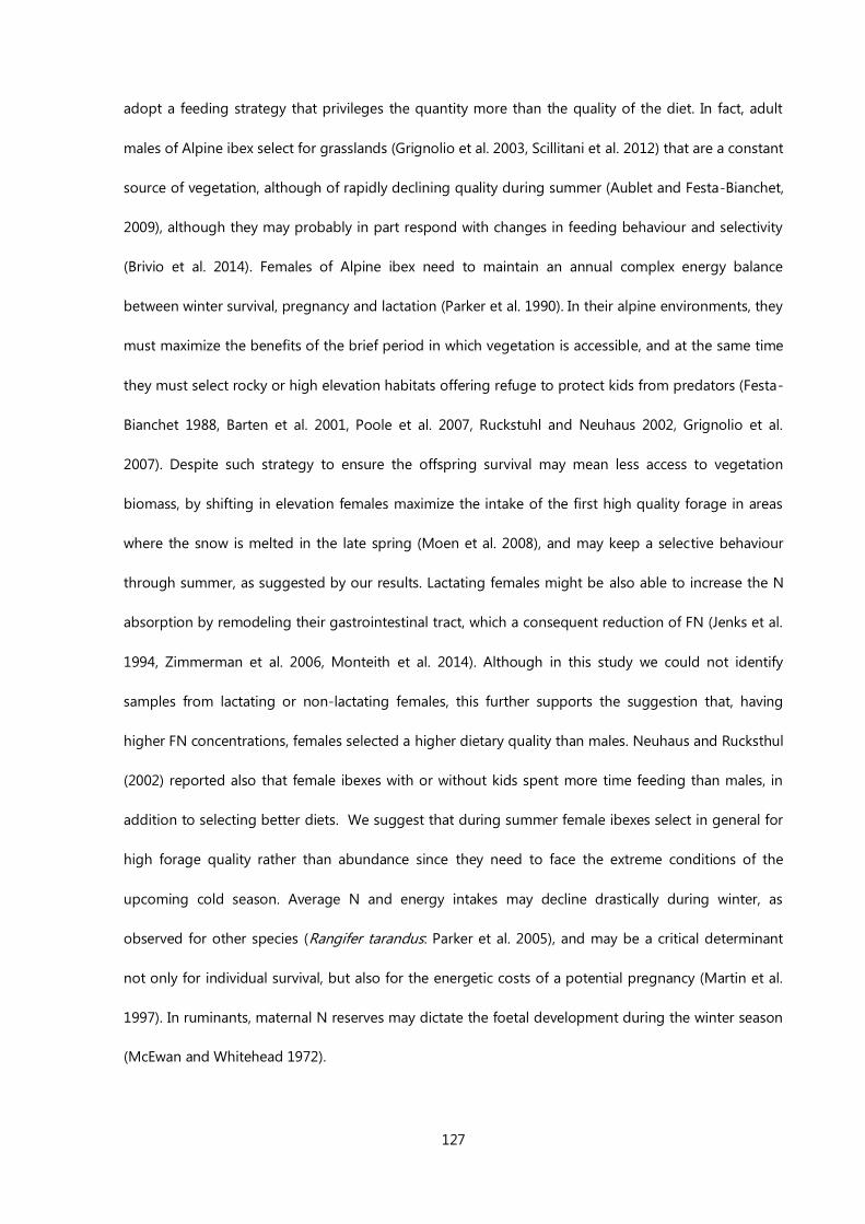
127
adopt a feeding strategy that privileges the quantity more than the quality of the diet. In fact, adult
males of Alpine ibex select for grasslands (Grignolio et al. 2003, Scillitani et al. 2012) that are a constant
source of vegetation, although of rapidly declining quality during summer (Aublet and Festa-Bianchet,
2009), although they may probably in part respond with changes in feeding behaviour and selectivity
(Brivio et al. 2014). Females of Alpine ibex need to maintain an annual complex energy balance
between winter survival, pregnancy and lactation (Parker et al. 1990). In their alpine environments, they
must maximize the benefits of the brief period in which vegetation is accessible, and at the same time
they must select rocky or high elevation habitats offering refuge to protect kids from predators (Festa-
Bianchet 1988, Barten et al. 2001, Poole et al. 2007, Ruckstuhl and Neuhaus 2002, Grignolio et al.
2007). Despite such strategy to ensure the offspring survival may mean less access to vegetation
biomass, by shifting in elevation females maximize the intake of the first high quality forage in areas
where the snow is melted in the late spring (Moen et al. 2008), and may keep a selective behaviour
through summer, as suggested by our results. Lactating females might be also able to increase the N
absorption by remodeling their gastrointestinal tract, which a consequent reduction of FN (Jenks et al.
1994, Zimmerman et al. 2006, Monteith et al. 2014). Although in this study we could not identify
samples from lactating or non-lactating females, this further supports the suggestion that, having
higher FN concentrations, females selected a higher dietary quality than males. Neuhaus and Rucksthul
(2002) reported also that female ibexes with or without kids spent more time feeding than males, in
addition to selecting better diets. We suggest that during summer female ibexes select in general for
high forage quality rather than abundance since they need to face the extreme conditions of the
upcoming cold season. Average N and energy intakes may decline drastically during winter, as
observed for other species (Rangifer tarandus: Parker et al. 2005), and may be a critical determinant
not only for individual survival, but also for the energetic costs of a potential pregnancy (Martin et al.
1997). In ruminants, maternal N reserves may dictate the foetal development during the winter season
(McEwan and Whitehead 1972).

128

129
Table 1. Results of calibrations with the BayesB model on the spectra obtained with the three methods. Results
(average, max and min) are from 15 replications, each with different calibration and validation sets.
Labspec
(350-1830 nm)
Foodscan
(850-1050 nm)
Labspec-FS
(850-1050 nm)
N NDF N NDF N NDF
R2TRN
a
Average 0.87 0.79 0.23 0.17 0.31 0.13
Max 0.93 0.85 0.31 0.24 0.42 0.27
Min 0.82 0.74 0.13 0.05 0.20 0.02
R2VAL
b
Average 0.72 0.59 0.23 0.07 0.33 0.07
Max 0.88 0.78 0.51 0.24 0.68 0.29
Min 0.40 0.38 0.02 0.00 0.00 0.00
RMSEVALc
Average 0.29 3.56 0.52 5.43 0.49 5.83
Max 0.35 4.61 0.66 7.20 0.65 7.49
Min 0.24 2.72 0.38 4.15 0.40 4.43
TRNd
115
115
115
115
116
116
TSTe
32
32
33
33
33
33
aR
2TRN= determination coefficient of TRN set calibration;
bR
2VAL= determination coefficient of validation;
cRMSEVAL= Root mean square error of validation;
dTRN= average number of samples in the 15 calibration sets;
eTST= average number of samples in the 15 calibration sets;
Table 2. Results of calibrations with the BayesB model on the spectra obtained with the three methods with the
entire dataset, and descriptive statistics of predicted values.
aR
2CAL= determination coefficient of calibration;
bRMSECAL= Root mean square error of calibration;
cTRN = number of samples in the calibration set;
d =valuesare given on an air-dried basis;
Labspec
(350-1830 nm)
FoodScan
(850.1050 nm)
Labspec-FS
(850-1050 nm) Chemical
N
NDF N NDF N NDF N NDF
R2CAL
a 0.88
0.78 0.24 0.18 0.32 0.09 -- --
RMSECALb 0.18
2.68 0.45 5.17 0.43 5.40 -- --
TRNc 147
147 148 148 143 149 -- --
Predicted valuesd
Average 2.47 43.47 2.44 43.78 2.37 43.67 2.42 43.78
Max 3.58 56.04 2.75 45.25 3.43 47.45 3.72 56.27
Min 1.63 30.75 2.25 37.16 1.93 38.80 1.44 29.93
SD 0.44 4.75 0.09 0.98 0.25 1.39 0.52 5.70

130
Table 3. parameters of the regression of FN and FNDF from chemical analysis on FN from NIRS methods. The P
values indicate the probability for intercept = 0 and b = 1.
Table 4. model selection for FN within Chemical and the different NIRs methods.
Table 5. Solution of fixed effects category and Julian date for the mixed linear models analysing FN data.
Intercept b
N% Mean ± SE P mean ± SE P
Chemical - LabSpec 0.026 ± 0.136 0.80 0.986 ± 0.055 0.85
Chemical - FoodScan -0.815 ± 0.660 0.21 1.335 ± 0.270 0.22
Chemical – LabSpec-FS -0.197 ± 0.144 0.58 1.069 ± 0.144 0.63
NDF%
Chemical - LabSpec 3.22 ± 2.75 0.23 0.931 ± 0.063 0.27
Chemical - FoodScan -50.86 ± 19.59 <0.01 2.162 ± 0.447 <0.01
Chemical – LabSpec-FS 10.54 ± 14.54 0.47 0.761 ± 0.333 0.47
Category Julian date NDVI AIC Δ AIC
Chemical
X X X 122.7 15.8
X X 106.9 0
X 108.8 1.9
LabSpec
X X X 94.7 17.7
X X 77.0 0.1
X 76.9 0
FoodScan
X X X -125.7 24.3
X X -146.0 4
X -150.0 0
LabSpec-FS
X X X -8.9 21.1
X X -27.2 2.8
X -30.0 0
l.s. estimate SE T P
Intercept
Chemical 4.731 0.366 12.94 <0.001
LabSpec 4.356 0.298 14.62 <0.001
Foodscan 2.898 0.110 26.31 <0.001
LabSpec -FS 2.952 0.234 12.61 <0.001
Females vs Males
Chemical 0.263 0.127 2.08 <0.05
LabSpec 0.165 0.103 1.61 0.118
Foodscan -0.033 0.038 -0.87 0.392
LabSpec -FS 0.052 0.081 0.64 0.528
Julian date
Chemical -0.0101 0.0015 -6.81 <0.001
LabSpec -0.0083 0.0012 -6.81 <0.001
Foodscan -0.0018 0.0004 -3.92 <0.001
LabSpec -FS -0.0022 0.0010 -2.32 <0.05
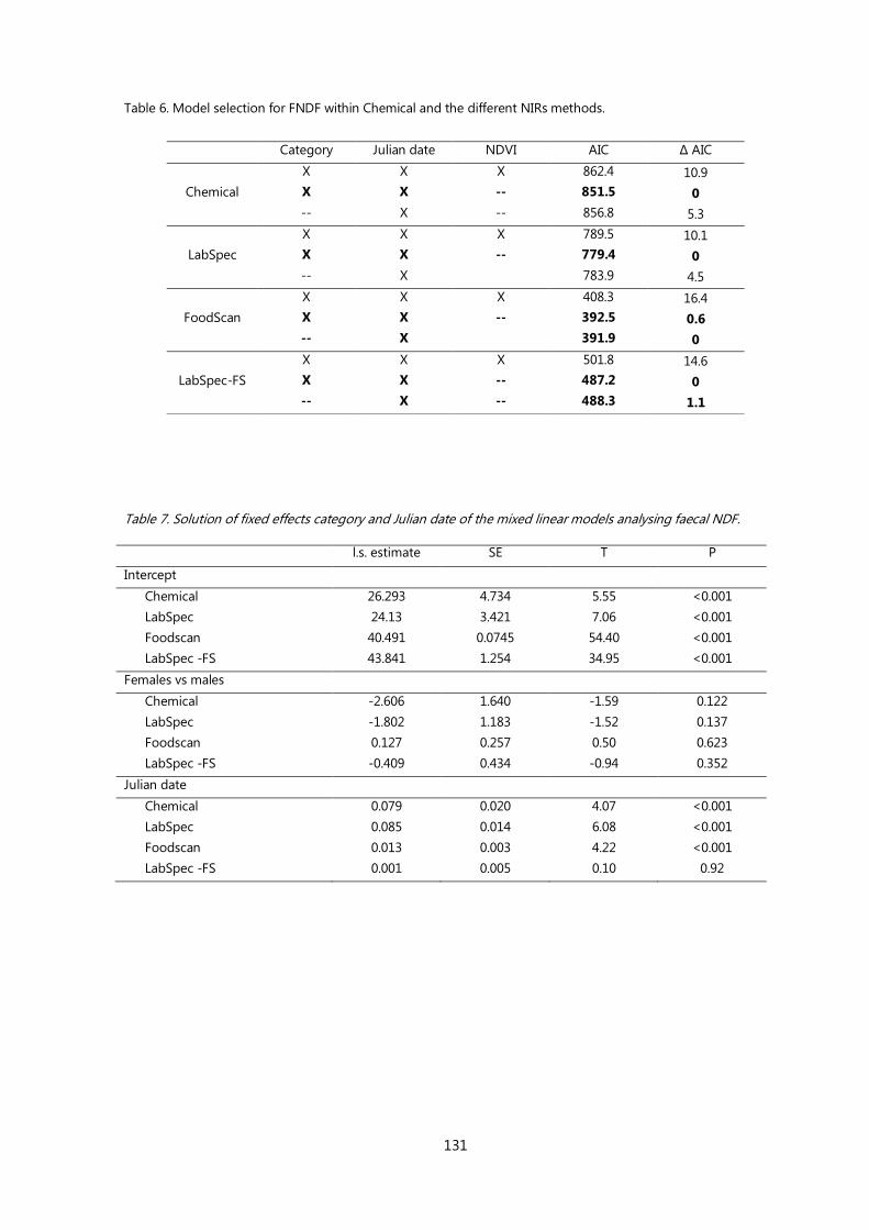
131
Table 6. Model selection for FNDF within Chemical and the different NIRs methods.
Table 7. Solution of fixed effects category and Julian date of the mixed linear models analysing faecal NDF.
l.s. estimate SE T P
Intercept
Chemical 26.293 4.734 5.55 <0.001
LabSpec 24.13 3.421 7.06 <0.001
Foodscan 40.491 0.0745 54.40 <0.001
LabSpec -FS 43.841 1.254 34.95 <0.001
Females vs males
Chemical -2.606 1.640 -1.59 0.122
LabSpec -1.802 1.183 -1.52 0.137
Foodscan 0.127 0.257 0.50 0.623
LabSpec -FS -0.409 0.434 -0.94 0.352
Julian date
Chemical 0.079 0.020 4.07 <0.001
LabSpec 0.085 0.014 6.08 <0.001
Foodscan 0.013 0.003 4.22 <0.001
LabSpec -FS 0.001 0.005 0.10 0.92
Category Julian date NDVI AIC Δ AIC
Chemical
X X X 862.4 10.9
X X -- 851.5 0
-- X -- 856.8 5.3
LabSpec
X X X 789.5 10.1
X X -- 779.4 0
-- X 783.9 4.5
FoodScan
X X X 408.3 16.4
X X -- 392.5 0.6
-- X 391.9 0
LabSpec-FS
X X X 501.8 14.6
X X -- 487.2 0
-- X -- 488.3 1.1

132
0
1
2
3
4
150 200 250 300 350
faecalN
Juliandate
Chemical
0
1
2
3
4
150 200 250 300 350
faecalN
Juliandate
VisNIR
0
1
2
3
4
150 200 250 300 350
faecalN
Juliandate
VisNIR-FS
0
1
2
3
4
150 200 250 300 350
faecalN
Juliandate
FoodScan
0
10
20
30
40
50
60
150 200 250 300 350
faecalN
DF
Juliandate
Chemical
0
10
20
30
40
50
60
150 200 250 300 350
faecalN
DF
Juliandate
VisNIR
0
10
20
30
40
50
60
150 200 250 300 350
faecalN
DF
Juliandate
FoodScan
0
10
20
30
40
50
60
150 200 250 300 350
faecalN
DF
Juliandate
VisNIR-FS
LabSpec
LabSpec-FS
Chemical
FoodScan
Figure 1. Julian date and trend of FN estimated with chemical and predicted with the three NIR methods
Figure 2. Julian date and trend of faecal NDF estimated with Chemical and predicted with the three NIR methods
LabSpec
LabSpec-FS
Chemical
Food Scan
LabSpec
LabSpec-FS
Chemical
FoodScan

133
LITERATURE CITED
Abbas, F., Morellet, N., Hewison, A. M., Merlet, J., Cargnelutti, B., Lourtet, B., ... and Verheyden, H.
(2011). Landscape fragmentation generates spatial variation of diet composition and quality in a
generalist herbivore. Oecologia, 167(2), 401-411.
Aernouts, B., Polshin, E., Lammertyn, J., and Saeys, W. (2011). Visible and near-infrared spectroscopic
analysis of raw milk for cow health monitoring: Reflectance or transmittance?. Journal of dairy science,
94(11), 5315-5329.
Aublet, J. F., Festa-Bianchet, M., Bergero, D., and Bassano, B. (2009). Temperature constraints on
foraging behaviour of male Alpine ibex (Capra ibex) in summer. Oecologia, 159(1), 237-247.
Baker, D. L., and Hobbs, N. T. (1987). Strategies of digestion: digestive efficiency and retention time of
forage diets in montane ungulates. Canadian Journal of Zoology, 65(8), 1978-1984.
Barbosa, I. C., Kley, M., Schäufele, R., Auerswald, K., Schröder, W., Filli, F., ... and Schnyder, H. (2009).
Analysing the isotopic life history of the alpine ungulates Capra ibex and Rupicapra rupicapra
rupicapra through their horns. Rapid Communications in Mass Spectrometry, 23(15), 2347-2356.
Barboza, P. S., and Bowyer, R. T. (2000). Sexual segregation in dimorphic deer: a new gastrocentric
hypothesis. Journal of Mammalogy, 81(2), 473-489.
Barten, N. L., Bowyer, R. T., and Jenkins, K. J. (2001). Habitat use by female caribou: tradeoffs associated
with parturition. The Journal of wildlife management, 77-92.
Beier, P. (1987). Sex differences in quality of white-tailed deer diets. Journal of Mammalogy, 323-329.
Berteaux, D., Crête, M., Huot, J., Maltais, J., and Ouellet, J. P. (1998). Food choice by white-tailed deer in
relation to protein and energy content of the diet: a field experiment. Oecologia, 115(1-2), 84-92.
Berzaghi, P., and Riovanto, R. (2010). Near infrared spectroscopy in animal science production:
principles and applications. Italian Journal of Animal Science, 8(3s), 39-62.
Blanchard, P., Festa-Bianchet, M., Gaillard, J. M., and Jorgenson, J. T. (2003). A test of long-term fecal
nitrogen monitoring to evaluate nutritional status in bighorn sheep. The Journal of wildlife
management, 477-484.
Borowik, T., Pettorelli, N., Sönnichsen, L., and ędrzejewska, B. (2013). Normalized difference vegetation
index (NDVI) as a predictor of forage availability for ungulates in forest and field habitats. European
Journal of Wildlife Research, 59(5), 675-682.
Bowyer, R. T. (1984). Sexual segregation in southern mule deer. Journal of Mammalogy, 410-417.
Bowyer, R. T. (2004). Sexual segregation in ruminants: definitions, hypotheses, and implications for
conservation and management. Journal of Mammalogy, 85(6), 1039-1052.
Bozdogan, H. (1987). Model selection and Akaike's information criterion (AIC): The general theory and
its analytical extensions. Psychometrika, 52(3), 345-370.
Brivio, F., Grignolio, S., Brambilla, A., and Apollonio, M. (2014). Intra-sexual variability in feeding
behaviour of a mountain ungulate: size matters. Behavioral Ecology and Sociobiology, 68(10), 1649-
1660.

134
Cebrian, M.R. et al 2008. Forge quality and reindeer productivity: multiplier effects amplified by climate
change.
Clarke, C. M. H., & Henderson, R. J. (1984). Home range size and utilization by female chamois
(Rupicapra rupicapra L.) in the Southern Alps, New Zealand. Acta Zoologica Fennica[ACTA ZOOL.
FENN.]. 1984.
Cook, R. C., Cook, J. G., Garrott, R. A., Irwin, L. L., and Monfort, S. L. (2002). Effects of diet and body
condition on fecal progestagen excretion in elk. Journal of wildlife diseases, 38(3), 558-565.
Cook, J. G., Johnson, B. K., Cook, R. C., Riggs, R. A., Delcurto, T., Bryant, L. D., and Irwin, L. L. (2004).
Effects of summer‐autumn nutrition and parturition date on reproduction and survival of elk. Wildlife
Monographs, 155(1), 1-61.
Côté, S. D., and Festa-Bianchet, M. (2001). Reproductive success in female mountain goats: the
influence of age and social rank. Animal Behaviour, 62(1), 173-181.
Crampe, J. P., Bon, R., Gerard, J. F., Serrano, E., Caens, P., Florence, E., & Gonzalez, G. (2007). Site fidelity,
migratory behaviour, and spatial organization of female isards (Rupicapra pyrenaica) in the Pyrenees
National Park, France. Canadian journal of zoology, 85(1), 16-25.
De los Campos, G., and P. Pérez Rodriguez. 2014. BGLR: Bayesian Generalized Linear Regression
(version 1.0.3). http://cran.r-project.org/web/packages/BGLR/index.html.
De Marchi, M., Penasa, M., Cecchinato, A., and Bittante, G. (2013). The relevance of different near
infrared technologies and sample treatments for predicting meat quality traits in commercial beef cuts.
Meat science, 93(2), 329-335.
Demment, M. W., and Van Soest, P. J. (1985). A nutritional explanation for body-size patterns of
ruminant and nonruminant herbivores. American Naturalist, 641-672.
Festa-Bianchet, M. (1988). Seasonal range selection in bighorn sheep: conflicts between forage quality,
forage quantity, and predator avoidance. Oecologia, 75(4), 580-586.
Fontana, F., Rixen, C., Jonas, T., Aberegg, G., and Wunderle, S. (2008). Alpine grassland phenology as
seen in AVHRR, VEGETATION, and MODIS NDVI time series-a comparison with in situ measurements.
Sensors, 8(4), 2833-2853.
Gálvez-Cerón, A., Serrano, E., Bartolomé, J., Mentaberre, G., Fernández-Aguilar, X., Fernández-Sirera, L.,
... and Albanell, E. (2013). Predicting seasonal and spatial variations in diet quality of Pyrenean chamois
(Rupicapra pyrenaica pyrenaica) using near infrared reflectance spectroscopy. European Journal of
Wildlife Research, 59(1), 115-121.
Grignolio, S., Parrini, F., Bassano, B., Luccarini, S., and Apollonio, M. (2003). Habitat selection in adult
males of Alpine ibex, Capra ibex ibex. Folia Zoologica, 52(2), 113-120.
Grignolio, S., Rossi, I., Bassano, B., and Apollonio, M. (2007). Predation risk as a factor affecting sexual
segregation in Alpine ibex. Journal of Mammalogy, 88(6), 1488-1497.
Hamel, S., Garel, M., Festa‐Bianchet, M., Gaillard, J. M., and Côté, S. D. (2009). Spring Normalized
Difference Vegetation Index (NDVI) predicts annual variation in timing of peak faecal crude protein in
mountain ungulates. Journal of Applied Ecology, 46(3), 582-589

135
Hanley, T. A. (1982). The nutritional basis for food selection by ungulates. Journal of Range
Management, 146-151.
Hernández, L., and Laundré, J. W. (2005). Foraging in the 'landscape of fear' and its implications for
habitat use and diet quality of elk Cervus elaphus and bison Bison bison. Wildlife Biology, 11(3), 215-
220.
Hofmann, R. R., and Nygren, K. (1992). Morphophysiological specialization and adaptation of the
moose digestive system. Alces Suppl, 1, 91-100.
Holechek J.L. 1982. Methods for determining the nutritive quality of range ruminant diets: a review.
Homolka e Heroldovà 2001. Native red deer and introduced chamois: foraging habits and competition
in a subalpine meadow-spruce forest area.
Huete, A., Didan, K., Miura, T., Rodriguez, E. P., Gao, X., and Ferreira, L. G. (2002). Overview of the
radiometric and biophysical performance of the MODIS vegetation indices. Remote sensing of
environment, 83(1), 195-213.
Jackson, R. D., and Huete, A. R. (1991). Interpreting vegetation indices. Preventive Veterinary Medicine,
11(3), 185-200.
Jianzhang, M., Junsheng, L., Zhaowen, J., and Mingbo, G. (1999). Nitrogen and fiber concentration in
rumen contents and feces contents of Mongolian gazelles. Journal of Forestry Research, 10(2), 103-
106.
Jean, P. O., Bradley, R. L., Giroux, M. A., Tremblay, J. P., and Côté, S. D. (2014). Near Infrared
Spectroscopy and Fecal Chemistry as Predictors of the Diet Composition of White-Tailed Deer.
Rangeland Ecology and Management, 67(2), 154-159.
Jenks, J. A., Leslie Jr, D. M., Lochmiller, R. L., and Melchiors, M. A. (1994). Variation in gastrointestinal
characteristics of male and female white-tailed deer: implications for resource partitioning. Journal of
Mammalogy, 1045-1053.
Justice, C. O., Vermote, E., Townshend, J. R., Defries, R., Roy, D. P., Hall, D. K., ... and Barnsley, M. J.
(1998). The Moderate Resolution Imaging Spectroradiometer (MODIS): Land remote sensing for global
change research. Geoscience and Remote Sensing, IEEE Transactions on, 36(4), 1228-1249.
Kamler, J., and Homolka, M. (2005). Faecal nitrogen: a potential indicator of red and roe deer diet
quality in forest habitats. FOLIA ZOOLOGICA-PRAHA-, 54(1/2), 89.
Kamler, J., and Homolka, M. (2011). Needles in faeces: an index of quality of wild ungulate winter diet.
Folia Zoologica, 60(1), 63-69.
Leite, E. R., and Stuth, J. W. (1995). Fecal NIRS equations to assess diet quality of free-ranging goats.
Small Ruminant Research, 15(3), 223-230.
Lendrum, P. E., Elbroch, L. M., Quigley, H., Thompson, D. J., Jimenez, M., and Craighead, D. (2014).
Home range characteristics of a subordinate predator: selection for refugia or hunt opportunity?.
Journal of Zoology.
Leslie Jr, D. M., and Starkey, E. E. (1987). Fecal indices to dietary quality: a reply. The Journal of wildlife
management, 321-325.

136
Leslie, D. M., and Starkey, E. E. (1985). Fecal indices to dietary quality of cervids in old-growth forests.
The Journal of wildlife management, 142-146.
Leslie Jr, D. M., Jenks, J. A., Chilelli, M., and Lavigne, G. R. (1989). Nitrogen and diaminopimelic acid in
deer and moose feces. The Journal of wildlife management, 216-218.
Loison, A., Festa-Bianchet, M., Gaillard, J. M., Jorgenson, J. T., and Jullien, J. M. (1999). Age-specific
survival in five populations of ungulates: evidence of senescence. Ecology, 80(8), 2539-2554
Lyons, R. K., and Stuth, J. W. (1992). Fecal NIRS equations for predicting diet quality of free-ranging
cattle. Journal of Range Management, 238-244.
Main, M. B., and Coblentz, B. E. (1996). Sexual segregation in Rocky Mountain mule deer. The Journal of
wildlife management, 497-507.
Main, M. B. (2008). Reconciling competing ecological explanations for sexual segregation in ungulates.
Ecology, 89(3), 693-704
Martin, M. E., and Aber, J. D. (1997). High spectral resolution remote sensing of forest canopy lignin,
nitrogen, and ecosystem processes. Ecological applications, 7(2), 431-443.
Martínez, T. (2002). Summer feeding strategy of Spanish ibex Capra pyrenaica and domestic sheep
Ovis aries in south-eastern Spain. Acta theriologica, 47(4), 479-490.
McEwan, E. H., and Whitehead, P. E. (1972). Reproduction in female reindeer and caribou. Canadian
journal of zoology, 50(1), 43-46.
Neuhaus, P., and Ruckstuhl, K. E. (2002). Foraging behaviour in Alpine ibex (Capra ibex): consequences
of reproductive status, body size, age and sex. Ethology Ecology and Evolution, 14(4), 373-381.
Meuwissen, T. H. E., B. J. Hayes, M. E. Goddard (2001). Prediction of total genetic value using Genome-
Wide Dense Marker Maps. Genetics. 157:1819-1829.
Miquelle, D. G., Peek, J. M., and Van Ballenberghe, V. (1992). Sexual segregation in Alaskan moose.
Wildlife Monographs, 3-57.
Moço, G., Serrano, E., Guerreiro, M., Ferreira, A. F., Petrucci-Fonseca, F., Maia, M. J., ... and Pérez, J. M.
(2013). Seasonal dietary shifts and selection of Iberian wild goat Capra pyrenaica Schinz, 1838 in
Peneda-Gerês National Park (Portugal). Galemys, 25, 12-27.
Moen, A. N. (1973). Wildlife ecology (p. 458). San Francisco: Freeman
Moen, J. (2008). Climate change: effects on the ecological basis for reindeer husbandry in Sweden.
AMBIO: A Journal of the Human Environment, 37(4), 304-311.
Monteith, K. B., Monteith, K. L., Bowyer, R. T., Leslie Jr, D. M., and Jenks, J. A. (2014). Reproductive
effects on fecal nitrogen as an index of diet quality: an experimental assessment. Journal of
Mammalogy, 95(2), 301-310.
Mysterud, A. (2000). The relationship between ecological segregation and sexual body size dimorphism
in large herbivores. Oecologia, 124(1), 40-54.

137
Mysterud, A., Langvatn, R., Yoccoz, N. G., and Chr, N. (2001). Plant phenology, migration and
geographical variation in body weight of a large herbivore: the effect of a variable topography. Journal
of Animal Ecology, 915-923.
Osborn, R. G., and Ginnett, T. F. (2001). Fecal nitrogen and 2, 6-diaminopimelic acid as indices to
dietary nitrogen in white-tailed deer. Wildlife Society Bulletin, 1131-1139
Parker, D. S. (1990). Manipulation of the functional activity of the gut by dietary and other means
(antibiotics/probiotics) in ruminants. The Journal of nutrition, 120(6), 639-648.
Parker, K. L., Barboza, P. S., and Stephenson, T. R. (2005). Protein conservation in female caribou
(Rangifer tarandus): effects of decreasing diet quality during winter. Journal of Mammalogy, 86(3), 610-
622.
Parker, K. L., Barboza, P. S., and Gillingham, M. P. (2009). Nutrition integrates environmental responses
of ungulates. Functional Ecology, 23(1), 57-69.
Pérez, P., and G. de los Campos. 2014. Genome Wide regression and prediction with the BGLR
statistical package. Genetics, July, DOI: 10.1534/genetics.114.164442.
Perez-Barberia, F. J., Perez-Fernandez, E., Robertson, E., and Alvarez-Enriquez, B. (2008). Does the
Jarman–Bell principle at intra-specific level explain sexual segregation in polygynous ungulates? Sex
differences in forage digestibility in Soay sheep. Oecologia, 157(1), 21-30.
Pettorelli, N., Ryan, S., Mueller, T., Bunnefeld, N., Jedrzejewska, B., Lima, M., and Kausrud, K. (2011). The
Normalized Difference Vegetation Index (NDVI): unforeseen successes in animal ecology. Climate
Research, 46(1), 15-27.
Pettorelli, N., Vik, J. O., Mysterud, A., Gaillard, J. M., Tucker, C. J., and Stenseth, N. C. (2005). Using the
satellite-derived NDVI to assess ecological responses to environmental change. Trends in ecology and
evolution, 20(9), 503-510.
Poole, K. G., Serrouya, R., and Stuart-Smith, K. (2007). Moose calving strategies in interior montane
ecosystems. Journal of Mammalogy, 88(1), 139-150.
Portier, C., Festa-Bianchet, M., Gaillard, J. M., Jorgenson, J. T., and Yoccoz, N. G. (1998). Effects of
density and weather on survival of bighorn sheep lambs (Ovis canadensis). Journal of Zoology, 245(03),
271-278.
R Core Team. 2013. R: A language and environment for statistical computing. R foundation for
Statistical Computing, Vienna, Austria. URL http://www.R-project.org/.
Robbins, C. (1983). Wildlife feeding and nutrition. Elsevier.
Robbins, C. T., Mole, S., Hagerman, A. E., and Hanley, T. A. (1987). Role of tannins in defending plants
against ruminants: reduction in dry matter digestion?. Ecology, 1606-1615.
Roberts, C. A., Stuth, J., and Flinn, P. (2004). Analysis of forages and feedstuffs. AGRONOMY, 231-268.
Ruckstuhl, K. E., and Neuhaus, P. (2000). Sexual segregation in ungulates: a new approach. Behaviour,
137(3), 361-377.
Ruckstuhl, K. E., and Neuhaus, P. (2002). Sexual segregation in ungulates: a comparative test of three
hypotheses. Biological Reviews of the Cambridge Philosophical Society, 77(01), 77-96.

138
Ryan, S. J., Cross, P. C., Winnie, J., Hay, C., Bowers, J., and Getz, W. M. (2012). The utility of normalized
difference vegetation index for predicting African buffalo forage quality. The Journal of Wildlife
Management, 76(7), 1499-1508.
Schultz, B. B. (1985). Levene's test for relative variation. Systematic Biology, 34(4), 449-456.
Schwarm, A., Schweigert, M., Ortmann, S., Hummel, J., Janssens, G. P. J., Streich, W. J., and Clauss, M.
(2009). No easy solution for the fractionation of faecal nitrogen in captive wild herbivores: results of a
pilot study. Journal of animal physiology and animal nutrition, 93(5), 596-605
Scillitani, L., Sturaro, E., Menzano, A., Rossi, L., Viale, C., and Ramanzin, M. (2012). Post-release spatial
and social behaviour of translocated male Alpine ibexes (Capra ibex ibex) in the eastern Italian Alps.
European Journal of Wildlife Research, 58(2), 461-472.
Showers, S. E., Tolleson, D. R., Stuth, J. W., Kroll, J. C., and Koerth, B. H. (2006). Predicting diet quality of
white-tailed deer via NIRS fecal profiling. Rangeland Ecology and Management, 59(3), 300-307
Signer, C., Ruf, T., and Arnold, W. (2011). Hypometabolism and basking: the strategies of Alpine ibex to
endure harsh over‐wintering conditions. Functional Ecology, 25(3), 537-547.
Steltzer, H., and Welker, J. M. (2006). Modeling the effect of photosynthetic vegetation properties on
the NDVI-LAI relationship. Ecology, 87(11), 2765-2772
Stuth, J., Jama, A., and Tolleson, D. (2003). Direct and indirect means of predicting forage quality
through near infrared reflectance spectroscopy. Field Crops Research, 84(1), 45-56.
Tolleson, D., Stuth, J., Bai, K., Mo, F., and Kronberg, S. (2007). Faecal near infrared reflectance
spectroscopy to predict diet quality for sheep. Small ruminant research, 68(3), 263-268.
Tucker, C. J., and Sellers, P. J. (1986). Satellite remote sensing of primary production. International
journal of remote sensing, 7(11), 1395-1416.
Tucker, C. J., Pinzon, J. E., Brown, M. E., Slayback, D. A., Pak, E. W., Mahoney, R., ... and El Saleous, N.
(2005). An extended AVHRR 8‐km NDVI dataset compatible with MODIS and SPOT vegetation NDVI
data. International Journal of Remote Sensing, 26(20), 4485-4498.
Van Soest, P. J. (1994). Nutritional ecology of the ruminant. Cornell University Press.
Van Soest, P. J. (1996). Allometry and ecology of feeding behavior and digestive capacity in herbivores:
a review. Zoo Biology, 15(5), 455-479.
Verheyden, H., Aubry, L., Merlet, J., Petibon, P., Chauveau-Duriot, B., Guillon, N., and Duncan, P. (2011).
Faecal nitrogen, an index of diet quality in roe deer Capreolus capreolus?. Wildlife Biology, 17(2), 166-
175
Villaret, J. C., and Bon, R. (1995). Social and spatial segregation in Alpine ibex (Capra ibex) in Bargy,
French Alps. Ethology, 101(4), 291-300.
Villaret, J. C., Bon, R., and Rivet, A. (1997). Sexual segregation of habitat by the alpine ibex in the French
Alps. Journal of Mammalogy, 1273-1281.
Walker, A. B., Parker, K. L., and Gillingham, M. P. (2006). Behaviour, habitat associations, and intrasexual
differences of female Stone's sheep. Canadian journal of zoology, 84(8), 1187-1201.

139
Watanabe, T., and Takatsuki, S. (1993). Comparison of nitrogen and fiber concentrations in rumen and
fecal contents of Sika deer. Journal of the Mammalogical Society of Japan, 18(1), 43-48.
Wehausen, J. D. (1995). Fecal measures of diet quality in wild and domestic ruminants. The Journal of
wildlife management, 816-823.
Wofford, H., Holechek, J. L., Galyean, M. L., Wallace, J. D., and Cardenas, M. (1985). Evaluation of fecal
indices to predict cattle diet quality. Journal of Range Management, 450-454
Wrench, J. M., Meissner, H. H., and Grant, C. C. (1997). Assessing diet quality of African ungulates from
faecal analyses: the effect of forage quality, intake and herbivore species. Koedoe, 40(1), 125-136
Zimmerman, T. J., Jenks, J. A., and Leslie Jr, D. M. (2006). Gastrointestinal morphology of female white-
tailed and mule deer: effects of fire, reproduction, and feeding type. Journal of Mammalogy, 87(3),
598-605.


141
GENERAL CONCLUSIONS


143
This thesis provides new knowledge about the limitations and benefits of GPS tracking for
monitoring large herbivores in Alpine landscapes, reports the first attempt, to my knowledge, to
describe temporal patterns of spatial behaviour and the complex of intrinsic and extrinsic factors that
influence them in Alpine ibex females, and evaluates a rapid and economic approach for assessing
indirectly diet quality.
In the first chapter, by combining stationary GPS collars tests with data from free-ranging
collared animals, I investigated on the habitat features affecting the probability of acquiring a location
and the accuracy of received locations, and aimed at understanding how these features might interact
with individual activity under different climatic conditions. To my knowledge, such kind of information
was very limited for Alpine habitats, where the rugged land morphology and the extreme seasonality
in climate shape habitat features and animals behaviour. With stationary trials I found, not surprisingly,
that the probability of receiving a location was mostly influenced by physical obstructions limiting the
proportion of the available sky, while accuracy was influenced also by land cover, with forest having a
negative effect as respect to open areas. However, using an approach derived from the data collected
on the free-ranging female ibexes to screen the acquired locations for outliers, I found that in properly
edited databases the accuracy of retained locations can be fairly good, within 10 m for 50% of
locations and 20 m for 75% of them. Therefore, limitations for the GPS-tracking technology in Alpine
landscape seem to derive more from the biased proportion of locations that are received and retained
across different habitats, than from their accuracy.
For this purpose, I used a database of over 90,000 attempted locations from free-ranging
females to assess how fix acquisition rate and quality (as indexed by the NAV 2D/3D codes) varied
throughout the year and the daytime, and which habitat, climatic, and behavioural factors influenced
them. I confirmed the negative effects of physical obstructions to sky view on the probabilities of
acquiring a location and of acquired locations to be in the 3D class, but, more interestingly, I found
that these probabilities followed intra-annual and daily patterns, being lower in winter than in summer
144
and during nightime than daytime. The intensity of activity of animals had a positive effect on the
probability of acquiring a fix and on the proportion of 3D acquired fixes. These probabilities, in
addition, increased in days without precipitations and with temperatures higher than average,
especially in winter. I explained these findings as the result of an interaction between animals activity,
habitats selections, and climate. Female ibex are more active during summer and, especially in winter,
during daytime and in days with favourable climate and weather conditions, When animals are active
they are more likely to use open instead than sheltered areas, thus explaining the patterns observed in
fix acquisition rate and quality.
Therefore, the locations received (and finally retained) from GPS – collared Alpine ibex, and
likely from other large herbivores living at high elevations, underestimate the use of habitats providing
shelter and may drop in periods of adverse weather. This must be taken into account not only when
studying habitat selection, but also when deciding temporal scales of home ranges estimates. For
instance, while in our ibex population daily home range estimates might be reliable in summer, they
could be biased in winter. Therefore, in the second chapter of my thesis I decided to use longer
temporal scales in order to compare intra-annual patterns of home range size. Finally, a general
conclusion of this first chapter is that, since GPS collars performance is the result of non-random
interactions between two components, the habitat features and how and when the animals use these
habitats, researchers should not only address the first component with stationary tests, but should also
attempt to understand, using data from free-ranging animals, how the behaviour of their species in the
specific of their study areas may influence the results.
In the second chapter, I examined temporal trends of weekly and monthly home ranges and
core areas and how they were influenced by climate, food resources and individual conditions. I found
marked intra-annual patterns that were positively correlated with daylight, but were more
synchronized with indexes of climate and vegetation phenology. When I analysed the HR and CA sizes
within seasons, I found that they were predominantly influenced by climatic variables in winter, and by

145
idexes of food resources in summer. These results suggested that female ibexes adopt an extremely
conservative strategy of spatial use, which in winter is shaped by the need of reducing the costs and
the risks associated with movement. Only when snow starts melting and vegetation to grow they start
moving, and expande their ranges presumably in order to include patches of vegetation in early stages
of phenology.
My results are, to my knowledge, the first insight with GPS technology and at detailed
temporal and spatial scales on the space use strategies of female ibex. These animals live in areas with
an extreme seasonality and their spatial strategies have evolved to survive through long winters.
Winter HRs and CAs are very small and most probably located in specific favourable locations that
must be conserved. However, female ibex need also to make the maximum of the food available
during the short summers, in order to recover from the winter and raise their kids. The suitability of
wintering and summering area for Alpine areas might be in the future challenged by global climate
changes. An increase in temperatures might modify the amount and temporal distribution of snow
accumulation and its melting, and the temporal and spatial patterns of vegetation phenology.
Therefore, understanding how the spatial strategies of female ibexes, and likely of other species of
high mountain herbivores, are shaped by climate and habitat constraints is fundamental to predict
how they could adapt to changes in these conditions and to devise effective conservation actions.
In the third chapter, I evaluated the use of faecal N estimated with NIRS approaches as a rapid
and economic tool to describe biological patterns of the diet quality of both female and male Alpine
ibex. I found that, provided a suitable NIRS technology is used, this approach can provide biologically
meaningful results. In addition, I found that, in the high elevation habitats that characterize the
environment of the Alpine ibex, where the availability of nutritional resources alternative to Alpine
grasslands is restricted, the species cannot contrast the decline in vegetation quality from summer to
autumn. This indirectly confirms that strategies to reduce energy costs are most important for the
species during the long winters, and that only spring-early summer seem to be seasons when the

146
benefits of increasing home range in search of better food may overcompensate the cost and the risks
associated with movement, as I suggested in the second chapter. Females showed a tendency for
higher indexes of diet quality than males, which suggests that the energy requirements of pregnancy
and lactation lead them to a greater feeding selectivity. The fact that NDVI of the area surrounding
faecal samples was unrelated wit indexes of diet quality might appear in contrast with the results of
the second chapter, where NDVI of HRs was negatively correlated with their size. Possibly, my results in
this third chapter might derive from an inability to correctly adapt the size of the buffer area to the
spatio-temporal shifts of the animals, or by the need for refining NDVI indexes to take into account the
disturbing effects of variable proportions of bare soil. These aspects should be investigated with larger
spatial and temporal datasets. More in general, my results emphasize the need for improving the
knowledge on foraging strategies of species living in highly seasonal environments, in order to better
understand drivers of spatial behaviour and ultimately of evolution of life-history traits.

147
ACKNOWLEDGEMENTS
Questo lavoro è stato possibile grazie al sostegno alla ricerca scientifica della Fondazione
Cassa di Risparmio del Veneto e Rovigo, la quale mi ha dato l’opportunità di ottenere una borsa di
studio destinata allo svolgimento di un progetto di dottorato in Italia sostenuta dall’Università di
Padova. Ringrazio anche la Regione del Veneto e in particolare la Sezione Caccia e Pesca per il
supporto finanziario alla ricerca. Il Corpo Forestale delo Stato - comando provinciale del Veneto,
Ufficio Territoriale per la Biodiversità (UTB) di Tarvisio e stazione di Canale d’Agordo - , e il Corpo di
Polizia Provinciale di Belluno hanno fornito un insostituibile supporto logistico e per la cattura degi
animali.
Vorrei ringraziare il mio supervisore, Maurizio Ramanzin, dal primo momento in cui mi ha dato
l’opportunità di fare questo dottorato seguendo uno dei progetti più belli ed emozionanti. Quel
giorno di estate sulla Marmolada presi una delle decisioni più significative della mia vita, e ad oggi non
riesco ad immaginare che altra strada avrei potuto intraprendere che mi portasse più vicino alle mie
passioni. Grazie per avermi dato la possibilità di vivere questa esperienza, per il fondamentale
sostegno durante i tre anni di lavoro e per la comprensione nei momenti più difficili. Ringrazio anche
Enrico Sturaro per avermi reso più facili i miei primi momenti in Italia, era l’unico capace di parlare la
mia lingua!, ma soprattutto per il suo grande aiuto sia in aspetti lavorativi che personali.
Ringrazio con tutto il mio cuore Luca Rossi per avere incrociato il mio cammino, deviandolo
verso l’esperienza più bella e intensa della mia vita. Ho avuto la fortuna di aver conosciuto una delle
persone più rappresentative e stimate nell’ambito faunistico ma allo stesso tempo in grado di
trasmettermi l’importanza dell’umiltà, della semplicità e del coraggio per raggiungere i propri sogni.
Un ringraziamento speciale vorrei dedicarlo ad Alberto De Luca, la persona senza la quale non
sarei mai riuscita a sorpassare ogni ostacolo, avendomi dimostrato non solo una eccezionale capacità
intellettuale, ma anche una enorme generosità. Nei momenti più difficili mi è stato sempre vicino,

148
anche nella lontananza. Mi ha spinto su dopo ogni caduta in un modo incondizionato, mi ha insegnato
infiniti aspetti tecnici sul lavoro, mi ha trasmesso preziose conoscenze ma soprattutto mi ha convinta a
guardare sempre avanti senza smettere di sorridere. Non potrò mai restituirgli tutto quanto la sua
amicizia ha significato per me.
Per il loro inestimabile aiuto vorrei anche ringraziare le persone che hanno dedicato il suo
tempo, sforzo e passione al lavoro svolto sulle cime della Marmolada. Sono stati giorni di intensa fatica
fisica e mentale, ma anche delle più indescrivibili sensazioni di libertà e unione con ogni singolo
elemento della Natura. Ho avuto la fortuna di vivere a più di 2.000 m di altitudine i momenti
assolutamente più emozionanti di tutto questo lavoro. Ringrazio Matteo Mosconi, per la sua
l’inesauribile energia e l’avermi regalato tante preziose fotografie, alcune delle quali utilizzate in questa
tesi. Ma soprattutto grazie a Mattia Ferramosca, per avermi aspettato in ogni curva di ogni ardua salita,
in tutti i sensi della vita, con infinita pazienza, forza e positività, sollevando il peso dalle mie spalle e
convinto dalla mia forza e capacità. Raggiungere la cima non sarebbe stato possibile senza di lui.
Quisiera dar un saludo especial a Encarna por demostrarme tanta fortaleza. A pesar de su
ganas de ayudarme y aprender, de colaborar en el proyecto y de disfrutar de cada momento, la mala
suerte se nos adelantó, pero me dió la oportunidad de conocer una persona esplendida y sobretodo
indestructible!
Un profondo ringraziamento lo dedico alle “squadre cattura” del Corpo Forestale dello Stato e
del Corpo di Polizia Provinciale di Belluno. Con loro ho vissuto dei momenti fra più divertenti e
appassionanti di tutto questo percorso. Mi hanno dimostrato come l’uomo a volte possa correre sulle
rocce più veloce di uno stambecco, e come la tua passione possa diventare il tuo modo di vivere.
Hanno svolto un lavoro fondamentale per questo progetto, il quale senza di loro non sarebbe stato
possibile nemmeno cominciare, ma hanno anche avuto la capacità di agevolare la fatica con il loro
entusiasmo e semplicità. Grazie tante, con tutto il mio sincero affetto, alla squadra di catture più
coraggiosa e che io abbia mai conosciuto.
149
Ringrazio Francesca Cagnacci e Ferdinando Urbano per aver messo a disposizione dei dati
fondamentali (NDVI) che hanno permesso un maggior approfondimento e conoscenza degli aspetti
ecologici e comportamentali dello stambecco alpino, ma anche per l’aiuto ricevuto durante i miei primi
passi nell’utilizzo di programmi di gestione di ampi database.
Ringrazio l’Agenzia Regionale per la Prevenzione e Protezione Ambientale del Veneto (ARPAV)
per la velocità e disponibilità con cui hanno procurato i dati meteorologici indispensabili per
raggiungere gran parte delle conclusioni di questo lavoro.
Ringrazio con tantissimo affetto tutti i meravigliosi colleghi e ormai cari amici che ho potuto
conoscere in questi tre anni, Eirini, Serena, Erika, Alessandro, Miriam, Francesco, e un lungo eccetera.
Non è mai semplice tornare al punto di partenza lasciando alle spalle tutto quello che conosci, ma loro
mi hanno fatto sentire come a casa dal primo momento, e la loro accoglienza sarà sempre
indimenticabile per me.
Aunque llegar a Italia supuso un antes y un después, muchas personas permanecen siempre
ahí, en mi pasado, presente y futuro, dándome la certeza de que los buenos amigos duran toda la vida.
Quisiera agradecer todo el apoyo a mi querida Isis, a Patri, a Gloria, a Marisol, y a tantas otras personas
que me han demostrado su cariño cuando más lo he necesitado a pesar de la distancia.
A mi madre y hermanas no solo quiero agradacerles el apoyo que he siempre recibido para
alcanzar mis metas, si no tambièn el pilar fundamental que han supuesto en los momentos más
dificiles. Doy las gracias a mi madre por su amor incondicional, la paciencia de tantas despedidas y la
fortaleza con la que a pesar de todo aún sonríe a cada instante de la vida. A mis hermanas, porque han
sido siempre mi punto de referencia y las piezas de un puzze capaz de afrontar cualquier obstáculo.
Finalmente quisiera agradecerlo todo a la persona que me trajo hasta aquí, a mi padre. Quiero
darle las gracias por transmitirme los valores más sólidos y fundamentales de mi vida, por
entusiasmarme con sus enseñanzas sobre cada planta, cada pequeño insecto, cada pájaro o cada

150
curva de los senderos que tantas veces recorrimos juntos, por haberme maravillosamente contagiado
su pasión por la Naturaleza antes incluso de aprender a caminar. Esta tesis la dedico a él, porque la
fuerza de cada uno de mis pasos ha tenido solo un objetivo, demostrarle que cada día estoy más cerca
de hacer realidad el sueño que un día compartimos.

151