GRAPH-BASED CODES

Nigel Boston

Abstract. This is a mini-course on graph-based codes, given at the Center for The-

oretical Sciences at Taipei, Taiwan, July 12-15, 2004. In practical coding theory, the

main challenge has been to find codes with rates close to channel capacity and withefficient encoding and decoding algorithms. Only recently was this accomplished,

theoretically for the binary erasure channel but only experimentally for the binary

symmetric and AWGN channels. The classes of codes are related to graphs withmessage passing along edges providing the decoding. Analyzing them and designing

them leads to interesting mathematics, much of it still unresolved.

0. Caveat

It is important for the mathematician approaching this material to come at itwith the right mindset. As mathematicians we often seek to impose what sort ofproblem we wish to tackle. Here in dealing with the fundamental problems thatreal-life channels throw up, we do not enjoy that luxury. In particular, note:

(1) Decoding algorithms matter. In fact, here they become the crucial issue, andrather than skip them as engineering rather than math, they should be viewed asa springboard towards new and interesting mathematical challenges.

(2) Low density parity-check (LDPC) and similar codes are currently a veryhot topic. Every new ISIT meeting or issue of IEEE Transactions in InformationTheory typically has more on this topic than any other (with the exception of specialissues, and with space-time codes, list decoding, and quantum error-correcting codesrunning it close).

(3) The minimum distance of a code does not play as crucial a role as it doesin classical coding theory. It is just one measure of how good a code is and notthe best one at that. A few low-weight codewords may be tolerable. On the otherhand, whereas low-complexity bounded distance decoders abound, a large minimumdistance does not guarantee transmission at rates close to capacity.

1. History

In 1948 Shannon set the bar [21]. He showed that each communication channelhas a capacity, i.e. a rate below but not above which reliable transmission ispossible. He proved the existence of codes of rates arbitrarily close to capacityfor which probability of error using Maximum Likelihood Decoding (MLD) goes

The author thanks the CTS and Winnie Li for their kind hospitality during his visit to Taiwanand NSF DMS-0300321 for support in completing this report.

Typeset by AMS-TEX

1

2 NIGEL BOSTON

to zero (in fact exponentially fast) as block length goes to infinity. This, however,was non-constructive, and so the hunt was then on to design codes with efficientencoding and decoding algorithms and which approach the channel capacity. For arandom linear code of length n, it takes time and space of about O(n2) to encode(using the generator matrix) which is not so bad, but the real problem is that MLDdecoding takes O(2n) operations (all codes below are binary). For LDPC codes weshall see that the belief propagation algorithm reduces this to O(n). In fact thesecodes are typically so long in practice, e.g. n = 50000, that the n2 in encodingbecomes the bigger issue, for which various ad hoc solutions exist.

The interesting thing is that solutions (full and partial) to the above problemhave been repeatedly rediscovered and it is only in recent years that a uniformdescription for these has been discovered. This is the theory of graphical models(aka Bayesian networks) and the corresponding codes are called graph-based codes.These have taken the coding theory world by storm, and now form the main topic ofmodern practical coding theory [18]. It should be noted, however, that unlike othertopics in mathematical coding theory the decoding algorithms are of paramountimportance.

The first answer to Shannon’s challenge was presented in Gallager’s 1960 Ph.D.thesis [9], which first defined LDPC codes and proposed iterative decoding meth-ods, but with lack of computational power then they were impractical and theirvalue went largely unrecognized at the time, except in the USSR with Zyablov-Pinsker [30] and Margulis [15]. In 1981, Tanner [25] rediscovered LDPC codes andgeneralized them by introducing the notion of a Tanner graph. None of these, evenin simulation, came close to capacity, and so it was a major shock in 1993 (or ayear later, when experts finally acknowledged the correctness of their results) whenBerrou, Glavieux, and Thitimajshima [4] presented the new powerful class of Turbocodes with decoding algorithms that came close to Shannon’s limit.

When this development finally settled in, Wiberg, Loeliger, and Koetter [28]responded by generalizing Tanner graphs to factor graphs by including state vari-ables, allowing the theory to subsume Viterbi decoding [27],[8]. It was soon realisedthat the sum-product algorithm being used was a version of Pearl’s belief propa-gation algorithm [16]. In fact the sum-product algorithm, operating by messagepassing in a factor graph, subsumes algorithms used in artificial intelligence, statis-tical mechanics, and signal processing. This theme of rediscovery again arose whenin 1999 MacKay [12] rediscovered and revitalized Gallager’s codes, with extensivesimulations and actual proofs that LDPC codes are very good.

Attention shifted to which graphs produce the best codes, with Sipser and Spiel-man [24] in the theoretical computer science community rediscovering LDPC codesand realising how code performance relates to expansion properties of the under-lying graph (something the Russians mentioned earlier had realised but also wastemporarily unlearned). In time, LDPC codes were overtaking Turbo codes, one ad-vantage of LDPC codes being that efficient encoders and decoders could be designedfor them. Luby, Mitzenmacher, Shokrollahi, Spielman, and Stemann [11] designedone such for the binary erasure channel (BEC), performed a rigorous analysis, andnoted how graphs with irregular degree distributions perform much better than thestate-of-the-art regular graphs. This was further analyzed [17] using techniques ofdensity evolution to obtain optimal degree distributions that for the BEC provablyanswer Shannon’s challenge and indeed in practice perform much better than andhave implementation advantages over Turbo codes. There is, for instance, an en-

GRAPH-BASED CODES 3

semble of rate 1/2 irregular LDPC codes for the AWGN channel that gets within0.0045 dB of Shannon capacity [5].

As noted earlier, the literature (IEEE Trans.) and conference proceedings arecurrently awash with papers on LDPC codes and related issues with fundamentalissues being whether the results for the BEC can be extended to other channels, theoptimization of irregular LDPC codes for channels of interest, their implementationin VLSI, and their combination with other technologies such as MIMO (multiple-input multiple-output) systems. Time will tell as to which of the current flood ofpapers is of greatest importance but one fascinating development is the discoveryby Koetter and Vontobel [10] of the relevance of graph covers and the introductionof the fundamental polytope. The point here is that these decoding algorithmsoperate locally and so cannot distinguish between a graph and some cover of it, thusyielding pseudo-codewords responsible for suboptimal behavior of the algorithms -the fundamental polytope tightly characterizes these pseudo-codewords.

2. Overview of Lectures

After this history and overview, we define what is meant by a channel and outlineShannon’s results on the existence of a channel capacity limiting the possible ratesof reiable information transmission, setting us our goal. There are now three aspectsof graph-based codes to be discussed. We begin with trellises and give the BCJR[2] or two-way or forward-backward algorithm for trellises, explaining its efficiencycompared with MLD. Then we introduce Tanner graphs and describe the beliefpropagation algorithm for the corresponding codes. At this point, the usefulnessof sparse graph codes, specifically LDPC codes, becomes clear from a complexitystandpoint. The third aspect, namely factor graphs, combines the trellis and Tannergraph approaches and there is a very general sum-product algorithm for generalgraph-based codes.

We next focus on the simplest channel, the BEC, where belief propagationamounts to a very straightforward algorithm, permitting detailed analysis by tech-niques such as density evolution. This leads to capacity-achieving ensembles ofLDPC codes thereby answering Shannon’s challenge, and we deduce the degreedistributions of the corresponding irregular graphs. We then discuss the role ofexpander graphs in this area, their strengths [15],[19] and weaknesses [14]. Finally,graph covers and the fundamental polytope are discussed.

For a mathematician knowing the basics of classical coding theory and wantingto learn more, the voluminous (468 pages!) online notes by Richardson and Ur-banke [18] give an exhaustive (and exhausting) description of these developments.The two survey papers by Shokrollahi [22],[23] give a very readable introductionfor mathematicians. There are other good introductions to the field, many refer-enced below, although these are often written for engineers or theoretical computerscientists. The reader might try, for instance, Sason’s course notes [20]. MacKay’swebsite [13] has plenty of useful examples, theory, and software, whereas the web-site of the company Flarion Technologies [7] displays another side of LDPC codes,namely their industrial applications.

2. Channels and Capacity

4 NIGEL BOSTON

Definition. A communication channel is a triple consisting of an input alphabetA, an output alphabet B, and for each pair a ∈ A, b ∈ B a real number P (b | a)between 0 and 1. P (b | a) should be thought of as the probability that b is received,given that a is transmitted. In particular, we impose the constraint

∑b∈B P (b |

a) = 1, reflecting the fact that if a is transmitted, something is received.

You might complain that in practice it may be that nothing is received, i.e. wehave an erasure. This however is modeled by the binary erasure channel (BEC) bymaking erasure one of the output symbols. Here, A = {0, 1} (throughout these talkswe focus on binary codes), B = {0, 1, e}, and P (b | a) = 1− p if b = a, = p if b = e,else = 0, where p is the probability of an erasure. The BEC is the simplest channelto work with and appears in many real-life situations, where feedback channels donot exist, such as satellite links, rendering retransmission infeasible, and where onesender serves many recipients, such as a multicast scenario.

Another basic channel is the binary symmetric channel (BSC), where the inputand output alphabets are both {0, 1} and each bit is flipped with probability p.Thus, P (b | a) = 1 − p if b = a, else = p. The theory of the BSC turns out to bemuch more challenging than that of the BEC.

Finally (although many other interesting channels, in particular nonsymmetricones have been devised; see e.g. Sason’s notes [20] ), there is the additive whiteGaussian noise (AWGN) channel. Here, A ⊆ R, B = R, and

P (b | a) = exp(−(b− a)2/2σ2)/(√

2πσ)

meaning that the error (noise) is normally distributed with mean 0 and standarddeviation σ.

All three channels above have practical significance, but there are advantagesto working with general channels, and indeed universal decoding where we seekalgorithms that work well regardless of the underlying channel assumption, whichmay be unknown, is a dream that has undergone much investigation. Since wewish to transmit more than one symbol, we consider memoryless channels definedby the channel output at some instant depending only on the channel input atthat instant, so that if a = a1...an is transmitted and b = b1...bn received, thenP (b | a) =

∏ni=1 P (bi | ai).

For a general discrete-input, memoryless channel, Shannon [21] in 1948 associ-ated a number called its capacity, using information theory, a subject he simulta-neously developed. For the BEC, its capacity is 1 − p. For the BSC, its capacityis 1 + p log2 p + (1 − p) log2(1 − p). For the AWGN, it is W log2(1 + S/N), whereW is the bandwidth of the channel in Hz, S is the signal power in Watts, andN is the total noise power of the channel in Watts. The quantity S/N is calledsignal-to-noise ratio and is often expressed in decibels, such that 10k is 10k dB.Shannon showed that if maximum likelihood decoding (MLD) (see below) is used,then the decoding error probability for any code of rate greater than the channelcapacity approaches 1, and that for any rate below capacity, there are codes of thatrate for which the decoding error probability decreases to zero exponentially fastin the block-length as the latter goes to infinity.

Since, however, random codes were used, Shannon’s result left open the ques-tion of how to construct explicit ensembles of codes approaching capacity, with

GRAPH-BASED CODES 5

efficient encoding and decoding algorithms. MLD for the BSC, for instance, is NP-complete [3]. For the BEC it is polynomial-time but still inefficient [6]. Shannon’sarguments show that there are sequences of linear codes with rates approaching ca-pacity and MLD error probability approaching zero. Using linear codes, encodingis polynomial-time but it is a major open question to find sequences of capacity-achieving linear codes for which MLD for the BSC is polynomial-time. We explainbelow how to solve this problem for the BEC using the sum-product decodingalgorithm.

3. Trellises and the Forward-Backward Algorithm

Definition. A trellis is a directed graph in which every node is at a well-defineddepth with respect to a beginning node.

These depths will also be called times, so that in Figure 1, the horizontal is atime axis. This figure gives a trellis associated to the [7, 4, 2]-code with parity-checkmatrix

H =

1 1 1 0 0 0 01 0 0 1 1 0 01 0 0 0 0 1 1

meaning that the code consists of the 24 length 7 binary vectors x satisfying Hx = 0.The code is recovered from the trellis by following all possible paths through thetrellis. In fact this is a minimal trellis, and given a code it is easy to constructa corresponding minimal trellis. The most important invariants of the trellis areits maximum width, here 4, called its state complexity σ, and its constraint lengthlog2(σ).

Figure 2 gives another example of a trellis, this time attached to the [4, 3, 2]-codeC consisting of all vectors of length 4 with even weight. It has state complexity 2and so constraint length 1. We consider in detail the problem of decoding using thiscode and see how useful the trellis approach is for this, with the state complexitydetermining its efficiency.

Suppose a codeword is transmitted over the BSC with bit-error probability p =0.1 and y = 0010 received. Let us compute the most likely 2nd component x2 ofthe transmitted codeword x. The probability that x2 = 0 given y is

P (x2 = 0 | y) =∑

x∈C,x2=0

P (y | x)P (x)P (y)

(1)

since by Bayes rule, each term on the righthandside gives the posterior probabilitythat x is the input, given that y is the output.

We compute that∑x∈C,x2=0

P (y | x)P (x) = (3p(1− p)3 + p3(1− p))/8 = 0.02745

since P (x) = 1/8 (there being 8 codewords) and since of the 4 codewords in C withx2 = 0, namely 0000, 1001, 1010, 0011, one (1001) agrees with y in only one placewhereas the other three agree in exactly three places.

6 NIGEL BOSTON

Likewise, we compute that∑x∈C,x2=1

P (y | x)P (x) = (3p3(1− p) + p(1− p)3)/8 = 0.00945

since of the 4 codewords in C with x2 = 1, namely 1100, 1111, 0101, 0110, only one(0110) agrees in three places, the rest in only one.

Overall, P (y) is the sum over all x in C of the P (y | x), so P (y) = 0.02745 +0.00945 = 0.0369. We now return to equation (1) and compute that P (x2 = 0 |y) = 0.02745/0.0369 = 0.744 and likewise P (x2 = 1 | y) = 0.00945/0.0369 = 0.256.Then Maximum-Posterior (MAP) decoding tells us that most likely x2 = 0 since0.744 > 0.256. The problem is that this is simply too much work, particularly forlarge codes where about n2k operations will be needed.

The BCJR (or two-way or forward-backward) algorithm on the associated trellisworks much better. Given received word y = 0010, we make a forward computationas given in Figure 3 and then a backward computation given in Figure 4. Tocompute e.g. P (x2 = 0 | y), we put these computations together as in Figure 5,focusing just on the 2nd portion of the trellis. The zeros are on the horizontal edgesand multiplying the node and edge values and adding gives:

P (x2 = 0 | y) = q(0.45× 0.45× 0.09 + 0.05× 0.45× 0.41) = 0.744

Likewise using the diagonals,

P (x2 = 1 | y) = q(0.45× 0.05× 0.41 + 0.05× 0.05× 0.09) = 0.256

Here q is a normalizing constant to make sure that the two above probabilities addup to 1 (in fact q = 27.1).

The fact that the answers agree with those obtained by direct calculation is easilychecked. Consider P (x2 = 0 | y). The edge value a = P (x2 = 0)P (y2 = 0 | x2 = 0),the forward values f0 = P (x1 = 0)P (y1 = 0 | x1 = 0), f1 = P (x1 = 1)P (y1 = 0 |x1 = 1), and the backward values b0 = P (y4 = 0 | x4 = 0)P (x3 = 0)P (y3 = 1 |x3 = 0) + P (y4 = 0 | x4 = 1)P (x3 = 1)P (y3 = 1 | x3 = 1), b1 = P (y4 = 0 | x4 =0)P (x3 = 1)P (y3 = 1 | x3 = 1) + P (y4 = 0 | x4 = 1)P (x3 = 0)P (y3 = 1 | x3 = 0).Then f0ab0 + f1ab1 runs through

∑c∈C,c2=0

3∏1

P (xi = ci)∏

P (yi = ri | xi = ci)

where r1 = 0, r2 = 0, r3 = 1, r4 = 0 denotes the received word. Since the channel ismemoryless, this is

∑x∈C,x2=0 P (x)P (y | x). If the trellis is simple, i.e. has small

state complexity/constraint length, then the forward-backward algorithm will beconsiderably quicker than the term-by-term approach given first.

Analyzing this further, one sees that the time savings come essentially fromusing the distributive law, namely ab + ac = a(b + c) where the first expres-sion requires two multiplications and an addition whereas the second only onemultiplication and one addition. Note that sum distributes over min (leadingto the “min-sum” algorithm, analogous to the sum-product algorithm), namelya+min(b, c) = min(a, b)+min(a, c). What we have ended up with is a comparison

GRAPH-BASED CODES 7

of the likelihood that x2 = 0 versus that x2 = 1, given the received word y. Muchof what follows is a massive generalization of this observation.

It is worth noting that there is a variant on trellises, namely tail-biting trellises, where the time axis is a circle rather than a line and codewords are given by thepaths that go round once meeting themselves. Improper paths that go around morethan once before closing are like the pseudo-codewords of section 10. The point isthat whereas regular trellises are constrained to be thin at each end and so widein the middle, tail-biting trellises tend to have more uniform width. For instance,whereas the [24, 12, 8]-binary Golay code requires a trellis of constraint length atleast 8, it has a tail-biting trellis of constraint length 4.

4. Tanner Graphs

Suppose that a binary linear code C has parity-check matrix H, i.e. C = {x |Hx = 0}. Suppose that C has length n and that H is an r × n matrix over F2.The rate of C is then at least (n− r)/n (some of the checks may be redundant).

Definition. The Tanner graph associated to H is a bipartite graph constructedby taking as its vertices two kinds of nodes, namely n message nodes (one for eachcomponent xi) and r check nodes (one for each parity check), and by an edge goingfrom a message node v to a check node c only when c involves v.

Note that the same code can have different realizations as a Tanner graph (orindeed as a trellis) by choosing different parity-check matrices for it.

For example, for the parity check matrix of the [7, 4, 2]-code given in the lastsection, C is the common solution of x1+x2+x3 = 0, x1+x4+x5 = 0, x1+x6+x7 = 0- call these c1, c2, c3. The associated Tanner graph is given in Figure 6. It is cycle-free, which will turn out to be a desirable property for belief propagation to allowindependence assumptions, but this is actually a rare occurrence. Most good codes,for instance the [7, 4, 3]-Hamming code, have no cycle-free realizations, although wecan reasonably approximate cycle-free Tanner graphs in practice by ensuring thegraph has some desirable properties, e.g. large girth, expansion properties, etc.This will be explored later.

One important property is that the graph be sparse since as with the trellisescomputations will take place along those edges. This is typically an informal notion,but if we wish to be precise, a sequence of r×n matrices is called sparse if rn tendsto infinity and the number of nonzero elements in these matrices is always less thankmax(r, n) for some k.

Definition. The codes constructed by taking sparse matrices as their parity-check matrices are called Low Density Parity-Check (LDPC) Codes, the centraltopic of study in these lectures. An (s, t) regular LDPC code is a linear code witha parity-check matrix H that has s ones in every column and t ones in every row.

If H is an r × n parity-check matrix of an (s, t) regular LDPC code, the totalnumber of ones rt = ns. The rate of the code is at least (n − r)/n = 1 − s/t,so for instance a (3, 6) regular LDPC code has rate ≥ 1/2 (typically not much

8 NIGEL BOSTON

larger). Irregular LDPC codes have parity-check matrices with variable numbers ofones in their rows/columns and correspondingly the vertices of their Tanner graphshave irregular degree distributions. They have overtaken regular LDPC codes inimportance since they can be designed to come closer to capacity.

Gallager’s construction of regular LDPC codes proceeds as follows. Suppose wewant a (3, 6) regular LDPC code. Suppose n is a multiple of 6. Make the first row11111100...0 of length n, the second row 00000011111100...0, and so on, for the firstn/6 rows. To get the next n/6 rows apply a random permutation of degree n tothe columns of the above n/6×n matrix, and a second random permutation yieldsthe final n/6 rows. This is the so-called random construction of an LDPC code. Insection 9 below we discuss the pros and cons of efforts at non-random construction.

5. Belief Propagation

Message-passing algorithms form a class of algorithms on Tanner graphs wherein one round “messages” are passed from message nodes to check nodes and fromcheck nodes to message nodes. In belief propagation, the “messages” are actuallyprobabilities (or “beliefs”) meant to represent whether the ith message node “be-lieves” it is a 0 or a 1. At each stage, each node decides what it is to send to anadjacent node by using all the information that the other adjacent nodes have sentit.

We begin with an example (from Wolf’s excellent presentation [29]). Considerthe 9× 12 parity-check matrix

H =

0 0 1 0 0 1 1 1 0 0 0 01 1 0 0 1 0 0 0 0 0 0 10 0 0 1 0 0 0 0 1 1 1 00 1 0 0 0 1 1 0 0 1 0 01 0 1 0 0 0 0 1 0 0 1 00 0 0 1 1 0 0 0 1 0 0 11 0 0 1 1 0 1 0 0 0 0 00 0 0 0 0 1 0 1 0 0 1 10 1 1 0 0 0 0 0 1 1 0 0

There are three ones per column and four ones per row and so this produces a (3, 4)regular LDPC code. It’s a [12, 3, 4]-code, whose codewords are

000000000000, 000011100001, 010101100101, 010110000100,

101001111011, 101010011010, 111100011110, 111111111111

Suppose a codeword x is transmitted and the channel initially yields the followingprobabilities that xi = 1, 1 ≤ i ≤ 12; 0.9, 0.5, 0.4, 0.3, 0.9, 0.9, 0.9, 0.9, 0.9, 0.9, 0.9, 0.9.The ith message node of the Tanner graph gets this ith initial estimate and thenbroadcasts it to its adjacent check nodes. Each check node then makes new es-timates based on what it has received from other message nodes and sends theseestimates back to the message nodes.

How does it make this estimate? Take the first check c1 given by x3 + x6 + x7 +x8 = 0. This check node receives the initial estimates p3, p6, p7, p8 from the 3rd,

GRAPH-BASED CODES 9

6th, 7th, and 8th message nodes respectively. It computes new estimates

p′3 = p6(1− p7)(1− p8) + p7(1− p6)(1− p8) + p8(1− p6)(1− p7) + p6p7p8

and likewise for p′6, p′7, p

′8. This formula is explained below (see (3)).

Then p′3 is sent back to the 3rd message node, p′6 to the 6th message node, andso on. This happens simultaneously from all check nodes to their adjacent messagenodes (this parallelism is a definite implementation advantage over Turbo codes).Thus the 3rd message node receives revised estimates from check nodes c1, c5, c9,and makes a further refined estimate itself.

How does it make the refinement? Suppose it receives pA, pB , pC from thosethree check nodes. The estimate it sends back to A is simply kp3pBpC , to B iskp3pApC , and to C is kp3pApB , where p3 is the initial channel estimate and k is anormalizing constant. To compute k we solve simultaneously p′ = kpApBpC , 1−p′ =k(1− pA)(1− pB)(1− pC) to get k = 1/(pApBpC +(1− pA)(1− pB)(1− pC)). Thisformula is explained below (see (2)).

The process is then iterated. Let us run the example. Using p3 = 0.4, p6 =0.9, p7 = 0.9, p8 = 0.9, we compute at c1 that p′3 = 0.756. Since c5 involves the1st, 3rd, 8th, and 11th message nodes and the initial estimates for the three otherthan the 3rd are again 0.9, check node c5 also sends p′3 = 0.756 back to the 3rdmessage node. Finally, c9 involves the 2nd, 3rd, 9th, and 10th message nodes, andit computes p′3 = 0.5.

Thus the 3rd message node receives from c1, c5, c9 the estimates 0.756, 0.756, 0.5respectively. What does it send back? The products of the channel estimate 0.4and the other two estimates give respectively 0.1512, 0.1512, 0.2286. These arenormalized using k = 3.1692 to 0.4792, 0.4792, 0.7245.

After about 22 or more rounds of this, every message node carries an estimatenegligibly lower than 1.000 and we conclude that the all ones codeword was trans-mitted. (In fact a hard decision after 4 rounds, comparing the estimates with 0.5,gives the same conclusion.) We now give the general method.

Definition. Given a binary random variable x, P (x = 0)/P (x = 1) will be calledthe likelihood of x, denoted L(x). Likewise, the conditional likelihood of x given ywill refer to P (x = 0 | y)/P (x = 1 | y), denoted L(x | y).

Likelihoods allow us to make hard decisions on x by seeing if L(x) is greaterthan or less than 1. Since additions are easier to handle than multiplications, thebest algorithms often employ log-likelihoods , i.e. log L(x), log L(x | y), i.e. theseare the “beliefs” passed along edges.

If y1, ..., yd are independent random variables, then

log L(x | y1, ..., yd) =d∑

i=1

log L(x | yi) (2)

There is a small trick now to computing log L(x1 + ... + xd | y1, ..., yd), where thexi and yi are binary random variables. Namely we use the easily checked fact that

2P (x1 + x2 = 0 | y1, y2)− 1 = (2P (x1 = 0 | y1)− 1)(2P (x2 = 0 | y2)− 1)

10 NIGEL BOSTON

yielding by induction that

2P (x1 + ... + xd = 0 | y1, ..., yd)− 1 =d∏

i=1

(2P (xi = 0 | yi)− 1)

Letting Li = L(xi | yi) = P (xi = 0 | yi)/(1 − P (xi = 0 | yi), we get thatP (xi = 0 | yi) = Li/(1 + Li), whence 2P (xi = 0 | yi) − 1 = (Li − 1)/(Li + 1).Combining with the previous paragraph gives

2P (x1 + ... + xd = 0 | y1, ..., yd)− 1 =d∏

i=1

(Li − 1)/(Li + 1)

which, if we set `i = log Li, the conditional log-likelihood, yields

2P (x1 + ... + xd = 0 | y1, ..., yd)− 1 =d∏

i=1

tanh(`i/2)

whence

log L(x1+...+xd = 0 | y1, ..., yd) = log((1+d∏

i=1

tanh(`i/2))/(1−d∏

i=1

tanh(`i/2))) (3)

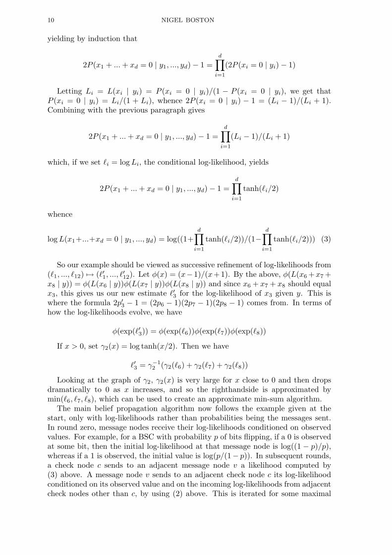
So our example should be viewed as successive refinement of log-likelihoods from(`1, ..., `12) 7→ (`′1, ..., `

′12). Let φ(x) = (x−1)/(x+1). By the above, φ(L(x6 +x7 +

x8 | y)) = φ(L(x6 | y))φ(L(x7 | y))φ(L(x8 | y)) and since x6 + x7 + x8 should equalx3, this gives us our new estimate `′3 for the log-likelihood of x3 given y. This iswhere the formula 2p′3 − 1 = (2p6 − 1)(2p7 − 1)(2p8 − 1) comes from. In terms ofhow the log-likelihoods evolve, we have

φ(exp(`′3)) = φ(exp(`6))φ(exp(`7))φ(exp(`8))

If x > 0, set γ2(x) = log tanh(x/2). Then we have

`′3 = γ−12 (γ2(`6) + γ2(`7) + γ2(`8))

Looking at the graph of γ2, γ2(x) is very large for x close to 0 and then dropsdramatically to 0 as x increases, and so the righthandside is approximated bymin(`6, `7, `8), which can be used to create an approximate min-sum algorithm.

The main belief propagation algorithm now follows the example given at thestart, only with log-likelihoods rather than probabilities being the messages sent.In round zero, message nodes receive their log-likelihoods conditioned on observedvalues. For example, for a BSC with probability p of bits flipping, if a 0 is observedat some bit, then the initial log-likelihood at that message node is log((1 − p)/p),whereas if a 1 is observed, the initial value is log(p/(1− p)). In subsequent rounds,a check node c sends to an adjacent message node v a likelihood computed by(3) above. A message node v sends to an adjacent check node c its log-likelihoodconditioned on its observed value and on the incoming log-likelihoods from adjacentcheck nodes other than c, by using (2) above. This is iterated for some maximal

GRAPH-BASED CODES 11

number of rounds or until the passed likelihoods are close to certainty, whicheveris first.

Since tanh can take on negative values, for which log is not defined, we letγ : [−∞,∞] → {±1} × [0,∞] be given by γ(x) = (sgn(x),− log tanh(|x|/2)). Sinceγ is bijective, there exists an inverse function γ−1. Then (3) is equivalent to

m(`)cv = γ−1(

d∑i=1

γ(m(`−1)vic ) (4)

where m(`)cv is the message passed from check node c to message node v in the `th

round, v1, ..., vd are the message nodes other than v adjacent to c, and m(`−1)vic is

the message passed from message node vi to check node c in the (`− 1)th round.Certainty is when a log-likelihood of +∞ (certainty of a 0) or of −∞ (certainty

of a 1) is received at a message node. The algorithm can run for a given number ofrounds or until certainty or near-certainty (given by some threshold) is obtained.

The decoding complexity of a round of the algorithm is proportional to thenumber of edges in the Tanner graph. This is why sparsity of the parity-checkmatrix is of paramount importance, and explains the value of LDPC codes. Forexample, for an (s, t) regular LDPC code, the Tanner graph has sn edges.

6. Factor Graphs and Generalized Distributive Laws

Wiberg and others [28] extended Tanner graphs to include invisible nodes, or“states”, thus creating a marriage of trellises and Tanner graphs. We call thesefactor graphs. Figure 7 shows the factor graph corresponding to the trellis givenin Figure 1, attached to a [7, 4, 2]-code. The states are represented by open circlesof different sizes, the check nodes represent the constraints governing a particulartrellis section, only certain pairs of neighboring states are allowed, and each allowedpair uniquely determines an associated code symbol. Note that the factor graphassociated to a trellis is always cycle-free.

The idea is that in computer science and engineering many algorithms deal withcomplicated “global” functions of many variables that can be efficiently computedby exploiting the way that the global function factors into a product of simple“local” functions. For example, suppose

g(x1, x2, x3, x4, x5) = fA(x1)fB(x2)fC(x1, x2, x3)fD(x3, x4)fE(x3, x5)

Figure 8 shows how the dependencies can be represented by a bipartite graphwith function nodes and variable nodes. We shall describe factor graphs that notonly encode the factorization of the global function but, when cycle-free, yield analgorithm, the sum-product algorithm, for computing marginal functions. In thecoding theory world, this was realised by Aji and McEliece [1] presented at Ulmin 1997, where corridor discussions among the so-called “Ulm group” crystallizedthe notion of factor graph, but the approach has broad application to Markovrandom fields, Bayesian networks (expertise in which was recently claimed to be anessential part of Microsoft’s competitive advantage by Bill Gates and which MITTechnology Review recently named one of the top ten emerging technologies), etc.

12 NIGEL BOSTON

These techniques are used e.g. in drug discovery, foreign-language translation, andmicrochip manufacturing.

Given global function g(x1, ..., xn), the marginal functions are defined by

gi(xi) :=∑

g(x1, ..., xn), 1 ≤ i ≤ n

meaning the sum over all variables other than xi. So, for instance, using thedistributive law,

g1(x1) = fA(x1)∑

x2,x3

(fB(x2)fC(x1, x2, x3)(∑x4

fD(x3, x4))(∑x5

fE(x3, x5))

Figure 9 shows how to represent this factorization and then add “not-sums” on theedges. When the factor graph is a tree, as here, by making xi the root, the factorgraph gives a message-passing algorithm for computing gi(xi), namely:

1. At a variable node xi, take the product of expressions formed at the descen-dants of xi.

2. At a function node f , take the product of f with expressions formed at thedescendants of f ; then perform the not-sum over the parent of f .

In coding theory, if we transmit x = x1...xn over a memoryless channel and ob-serve y = y1...yn, then the a posteriori joint probability distribution of {x1, ..., xn}is proportional to

P (x1, ..., xn) =∏

A∈G

PA(xA)n∏

i=1

P (yi | xi)

so computing it amounts to a sum-product algorithm on a corresponding factorgraph. As a simple example, consider the parity-check matrix H of the [7, 4, 2]-codeC considered above. Let f be the characteristic function of C, so that f(x) = 1if Hx = 0 and is 0 otherwise. Letting χ(x, y, z) = 1 if x + y + z = 0 and be 0otherwise, the global function f factors into local functions as

f(x1, ..., x7) = χ(x1, x2, x3)χ(x1, x4, x5)χ(x1, x6, x7)

7. Density Evolution on the Binary Erasure Channel

The following example is taken from [18]. Let

H =

0 0 0 0 1 0 0 0 1 1 1 0 0 0 0 1 0 0 0 10 0 0 0 0 0 1 1 0 0 1 1 0 1 0 1 0 0 0 00 1 1 0 0 0 1 0 0 0 0 0 0 0 0 1 0 1 0 10 0 0 0 0 1 0 1 0 1 0 0 0 0 0 0 1 1 1 01 1 0 0 1 0 0 0 0 0 0 0 1 0 0 0 1 0 1 00 0 0 0 0 0 1 0 0 0 1 1 0 1 1 0 0 0 0 10 0 0 1 1 1 0 1 0 0 0 0 1 0 1 0 0 0 0 01 0 1 0 0 0 0 0 1 0 0 0 1 1 1 0 0 0 0 01 1 1 1 0 0 0 0 0 1 0 0 0 0 0 0 1 0 0 00 0 0 1 0 1 0 0 1 0 0 1 0 0 0 0 0 1 1 0

GRAPH-BASED CODES 13

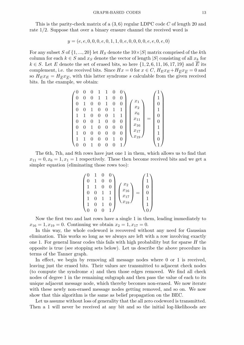
This is the parity-check matrix of a (3, 6) regular LDPC code C of length 20 andrate 1/2. Suppose that over a binary erasure channel the received word is

y = (e, e, 0, 0, 0, e, 0, 1, 1, 0, e, 0, 0, 0, 0, e, e, 0, e, 0)

For any subset S of {1, ..., 20} let HS denote the 10×|S|matrix comprised of the kthcolumn for each k ∈ S and xS denote the vector of length |S| consisting of all xk fork ∈ S. Let E denote the set of erased bits, so here {1, 2, 6, 11, 16, 17, 19} and E itscomplement, i.e. the received bits. Since Hx = 0 for x ∈ C, HExE +HExE = 0 andso HExE = HExE , with this latter syndrome s calculable from the given receivedbits. In the example, we obtain:

0 0 0 1 1 0 00 0 0 1 1 0 00 1 0 0 1 0 00 0 1 0 0 1 11 1 0 0 0 1 10 0 0 1 0 0 00 0 1 0 0 0 01 0 0 0 0 0 01 1 0 0 0 1 00 0 1 0 0 0 1

x1

x2

x6

x11

x16

x17

x19

=

1101001101

The 6th, 7th, and 8th rows have just one 1 in them, which allows us to find that

x11 = 0, x6 = 1, x1 = 1 respectively. These then become received bits and we get asimpler equation (eliminating those rows too):

0 1 0 00 1 0 01 1 0 00 0 1 11 0 1 11 0 1 00 0 0 1

x2

x16

x17

x19

=

1100110

Now the first two and last rows have a single 1 in them, leading immediately to

x16 = 1, x19 = 0. Continuing we obtain x2 = 1, x17 = 0.In this way, the whole codeword is recovered without any need for Gaussian

elimination. This works so long as we always are left with a row involving exactlyone 1. For general linear codes this fails with high probability but for sparse H theopposite is true (see stopping sets below). Let us describe the above procedure interms of the Tanner graph.

In effect, we begin by removing all message nodes where 0 or 1 is received,leaving just the erased bits. Their values are transmitted to adjacent check nodes(to compute the syndrome s) and then those edges removed. We find all checknodes of degree 1 in the remaining subgraph and then pass the value of each to itsunique adjacent message node, which thereby becomes non-erased. We now iteratewith these newly non-erased message nodes getting removed, and so on. We nowshow that this algorithm is the same as belief propagation on the BEC.

Let us assume without loss of generality that the all zero codeword is transmitted.Then a 1 will never be received at any bit and so the initial log-likelihoods are

14 NIGEL BOSTON

mv = +∞ if 0 is received at v, else is 0 (since an erased bit is equally likely to comefrom a 0 or a 1 according to the BEC model). The update equations tell us thefollowing (noting that γ2(+∞) = 0 and γ2(0) = +∞. If v is not erased, then mvc

is always +∞. If v is erased, then mvc = +∞ if and only if there is a check nodeadjacent to v other than c which sent +∞ to v in the previous round. mcv = +∞if and only if all the message nodes adjacent to c excluding v are not erased, else itequals 0.

Thus, the messages sent are binary (+∞ or 0) and by agreeing to delete messagesand edges once they carry a +∞, i.e. certainty, then we recover the algorithmgiven above. We can also very effectively analyze the algorithm by considering theproportion of edges carrying a 0 and seeing if this proportion approaches zero overtime (in which case our certainty approaches 100 percent. This is density evolution[17],[18].

A stopping set in the graph is a set of message nodes such that the graph inducedby these message nodes has the property that no check node has degree one. Theabove algorithm for the BEC stops prematurely, i.e. without recovering all themessage nodes, if and only if this subgraph has a stopping set. Unions of stoppingsets are stopping sets, and so every finite graph contains a unique maximal stoppingset (possibly empty). The size of a stopping set actually provides a lower boundfor the minimum distance of the code.

As for density evolution, let λd be the probability that an edge is connected toa message node of degree d and ρd be the probability that an edge is connectedto a check node of degree d. The generating functions λ(x) =

∑d λdx

d−1, ρ(x) =∑d ρdx

d−1 are critical in evaluating an LDPC code. For an (s, t) regular LDPCcode, λ(x) = xs−1, ρ(x) = xt−1, but it will turn out that more complicatedλ(x), ρ(x) are desirable, explaining the value of irregular LDPC codes.

Let pi be the probability that the message passed from a message node to acheck node at round i of the algorithm is 0. Let qi be the probability that themessage passed from a check node to a message node at round i is 0. A messagefrom a message node v to a check node c is 0 if and only if v was erased and allthe messages coming from the neighboring check nodes other than c are 0, which isqd−1i (assuming independence and that the degree of v is d) and so pi+1 = pqd−1

i .The check node c sends message ∞ to the message node v if and only if all theneighboring message nodes except for v send a message to ∞ to c the previousround, and so qi = 1 − (1 − pi)d−1, where here d is the degree of c. Putting thesetogether,

pi+1 = pλ(1− ρ(1− pi)) (5)

This is the critical equation. Suppose e.g. we have a (3, 6) regular LDPC code, sothat λ(x) = x2, ρ(x) = x5. Consider p0 = p = 0.4; we successively compute p1, p2, ...to be 0.3402, 0.3062, 0.2818, 0.2617, 0.2438, 0.2266, ... If, however, we start with p0 =p = 0.45, then we successively get 0.4058, 0.3858, 0.3748, 0.3681, 0.3639, 0.3612, ... Inthe first case, the numbers tend to 0, whereas the latter tend to 0.3554 The firstwill lead to successful decoding, the second unsuccessful. Further experimentationshows that the cut-off in behavior is at p = 0.42944. This is illustrated by thegraphs in Figure 10 for p = 0.4, 0.42944, 0.45.

This value of p is called the threshold and can be determined graphically or bythe following theorem. It has also been observed experimentally in simulations to

GRAPH-BASED CODES 15

be the correct cut-off point.

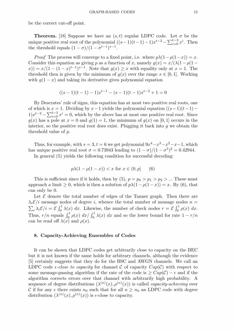
Theorem. [18] Suppose we have an (s, t) regular LDPC code. Let σ be theunique positive real root of the polynomial ((s−1)(t−1)−1)xt−2−

∑t−3i=0 xi. Then

the threshold equals (1− σ)/(1− σt−1)s−1.

Proof The process will converge to a fixed point, i.e. where pλ(1−ρ(1−x)) = x.Consider this equation as giving p as a function of x, namely g(x) = x/(λ(1−ρ(1−x)) = x/(1− (1− x)t−1)s−1. Note that g(x) ≥ x with equality only at x = 1. Thethreshold then is given by the minimum of g(x) over the range x ∈ [0, 1]. Workingwith g(1− x) and taking its derivative gives polynomial equation

((s− 1)(t− 1)− 1)xt−1 − (s− 1)(t− 1)xt−2 + 1 = 0

By Descrates’ rule of signs, this equation has at most two positive real roots, oneof which is x = 1. Dividing by x−1 yields the polynomial equation ((s−1)(t−1)−1)xt−2−

∑t−3i=0 xi = 0, which by the above has at most one positive real root. Since

g(x) has a pole at x = 0 and g(1) = 1, the minimum of g(x) on [0, 1] occurs in theinterior, so the positive real root does exist. Plugging it back into g we obtain thethreshold value of p.

Thus, for example, with s = 3, t = 6 we get polynomial 9x4−x3−x2−x−1, whichhas unique positive real root σ = 0.73943 leading to (1− σ)/(1− σ5)2 = 0.42944.

In general (5) yields the following condition for successful decoding:

pλ(1− ρ(1− x)) < x for x ∈ (0, p] (6)

This is sufficient since if it holds, then by (5), p = p0 > p1 > p2 > ... These mustapproach a limit ≥ 0, which is then a solution of pλ(1−ρ(1−x)) = x. By (6), thatcan only be 0.

Let E denote the total number of edges of the Tanner graph. Then there areλiE/i message nodes of degree i, whence the total number of message nodes n =∑

i λiE/i = E∫ 1

0λ(x) dx. Likewise, the number of check nodes r = E

∫ 1

0ρ(x) dx.

Thus, r/n equals∫ 1

0ρ(x) dx/

∫ 1

0λ(x) dx and so the lower bound for rate 1 − r/n

can be read off λ(x) and ρ(x).

8. Capacity-Achieving Ensembles of Codes

It can be shown that LDPC codes get arbitrarily close to capacity on the BECbut it is not known if the same holds for arbitrary channels, although the evidence[5] certainly suggests that they do for the BSC and AWGN channels. We call anLDPC code ε-close to capacity for channel C of capacity Cap(C) with respect tosome message-passing algorithm if the rate of the code is ≥ Cap(C)− ε and if thealgorithm corrects errors over that channel with arbitrarily high probability. Asequence of degree distributions (λ(n)(x), ρ(n)(x)) is called capacity-achieving overC if for any ε there exists n0 such that for all n ≥ n0 an LDPC code with degreedistribution (λ(n)(x), ρ(n)(x)) is ε-close to capacity.

16 NIGEL BOSTON

Major Open Question. Is there a channel other than the BEC and a message-passing algorithm for which there exists a capacity-achieving sequence?

Here is how the question is answered for the BEC with erasure probability p [17].Let ε > 0 be given and D be the ceiling of 1/ε. Let H(D) denote the harmonicsum

∑Di=1 1/i. Set λ(x) = (1/H(D))

∑Di=1 xi/i and ρ(x) = exp(µ(x − 1)), where

µ = H(D)/p (actually not a polynomial but it can be arbitrarily well approximatedby polynomials). Note that these are legitimate degree distributions since λ(1) =1, ρ(1) = 1 and their coefficients lie between 0 and 1.

Since λ(x) < (−1/H(D)) log(1− x) (by completing the power series),

pλ(1− ρ(1− x)) < (−p/H(D)) log ρ(1− x) = (µp/H(D))x = x

establishing (6). The rate of these codes is at least 1−r/n = 1−∫ 1

0ρ(x) dx/

∫ 1

0λ(x) dx =

1− p(1 + 1/D)(1− e−µ), which exceeds 1− p(1 + ε). Recalling that the BEC hascapacity 1−p, this shows that the LDPC codes with the above degree distributions(called Tornado codes for commercial appeal) are ε-close to capacity (and by (6)the belief propagation algorithm corrects errors arbitrarily well). We conclude that:

Theorem. [17] For the binary erasure channel, there exists a family of LDPCcodes whose rates approach capacity and which can be decoded by belief propaga-tion with arbitrarily small probability of error, i.e. Shannon’s challenge is answeredfor the BEC.

For other channels belief propagation can be quite complicated and so sometimesa discretized version is employed with the messages made binary, as they are withthe BEC.

9. Graphs of Large Girth, Expander Graphs and LDPC Codes

Attention shifts to what sorts of Tanner graphs are best for decoding. After `rounds message-passing travels at most 2` edges from any node and so stays withinthe ball of radius 2` about that node. If for all the vertices these balls are trees, thenthe graph has girth (i.e. smallest cycle length) > 2` but in practice it is enoughthat this holds for most nodes. Theoretical computer science has arguments toshow that the actual behavior of the algorithm is sharply concentrated around itsexpectation.

For fixed ` and large enough n, r, for random bipartite graphs the neighborhoodof depth ` of most of the message nodes is a tree. If (6) holds, then for any ε > 0,there exists n0 such that for all n ≥ n0, the BEC algorithm given reduces thenumber of erased message nodes below size εn. To get further, we introduce thefollowing.

Definition. A bipartite graph with n message nodes is an (α, β)-expander if forany subset S of the message nodes of size ≤ αn the number of neighbors of S is≥ βaS |S|, where aS is the average degree of the nodes in S.

GRAPH-BASED CODES 17

One can show that if the Tanner graph is an (ε, 1/2)-expander, then the BECalgorithm recovers any set of εn or fewer erasures, and so we are done.

As noted earlier, if there is no cycle of length ≤ 2`, then the independenceassumption is valid for ` rounds of belief propagation. In particular, for theserounds density evolution describes exactly the expected behavior of the densityfunctions. The girth of a graph is clearly even for bipartite graphs and can beupper bounded in the following way:

Theorem. Consider an (s, t) regular LDPC code with block length n = rt/s.Let α = (s− 1)(t− 1). If the girth c ≡ 2 (mod 4), then c ≤ 4 logα r + 2.

Proof Starting at a check node, count the number of check nodes reached afterat most (c− 2)/4 steps. These are all distinct, yielding the inequality

1 + t(s− 1) + t(s− 1)α + ... + t(s− 1)α(c−2)/4−1 ≤ r

Replacing t by t− 1 in the lefthandside gives

1 + α + α2 + ... + α(c−2)/4 = (α(c−2)/4+1 − 1)/(α− 1) ≤ r

from which the result follows.

Note also that a word of weight d leads to a cycle of length at most 2d in theTanner graph, but not vice versa (leading to pseudo-codewords as studied in thenext section). Thus the girth of a graph is akin to the minimum distance of a code,and just as codes can withstand having a few low-weight codewords, a few shortcycles don’t necessarily hurt the decoding. Ramanujan graphs, which have largegirth in an asymptotic sense, are now considered, their importance to LDPC codeshaving been recognized as long ago as Margulis’ paper [15].

Definition. A Ramanujan graph is a finite, connected k-regular graph such thatµ1 ≤ 2

√k − 1 where µ1 is the largest nontrivial eigenvalue of the adjacency matrix

of the graph.

There are many ways to construct Ramanujan graphs, the following methodbeing due to Margulis. Let q be an odd prime and PGL2(Fq) the quotient group of2× 2 invertible matrices over Fq modulo scalars. This group has order q3− q. Theprojective special linear group PSL2(Fq) coming from determinant one matriceshas index 2 in PGL2(Fq). Suppose now p < q are primes that are 1 (mod 4) withp a quadratic nonresidue mod q. By Jacobi, p = a2

0 + a21 + a2

2 + a23 has exactly p+1

solutions with a0 odd and greater than zero and aj even for j = 1, 2, 3. Let i ∈ Fq

satisfy i2 = −1. For each of the p + 1 solutions, define a matrix(a0 + ia1 a2 + ia3

−a2 + ia3 a0 − ia1

)Let X be the set of all such matrices.

The Cayley graph of PGL2(Fq) with respect to X is then a p+1-regular bipartiteRamanujan graph with q3 − q vertices and girth c ≥ 4 logp q − logp 4. We build acorresponding LDPC code as follows.

18 NIGEL BOSTON

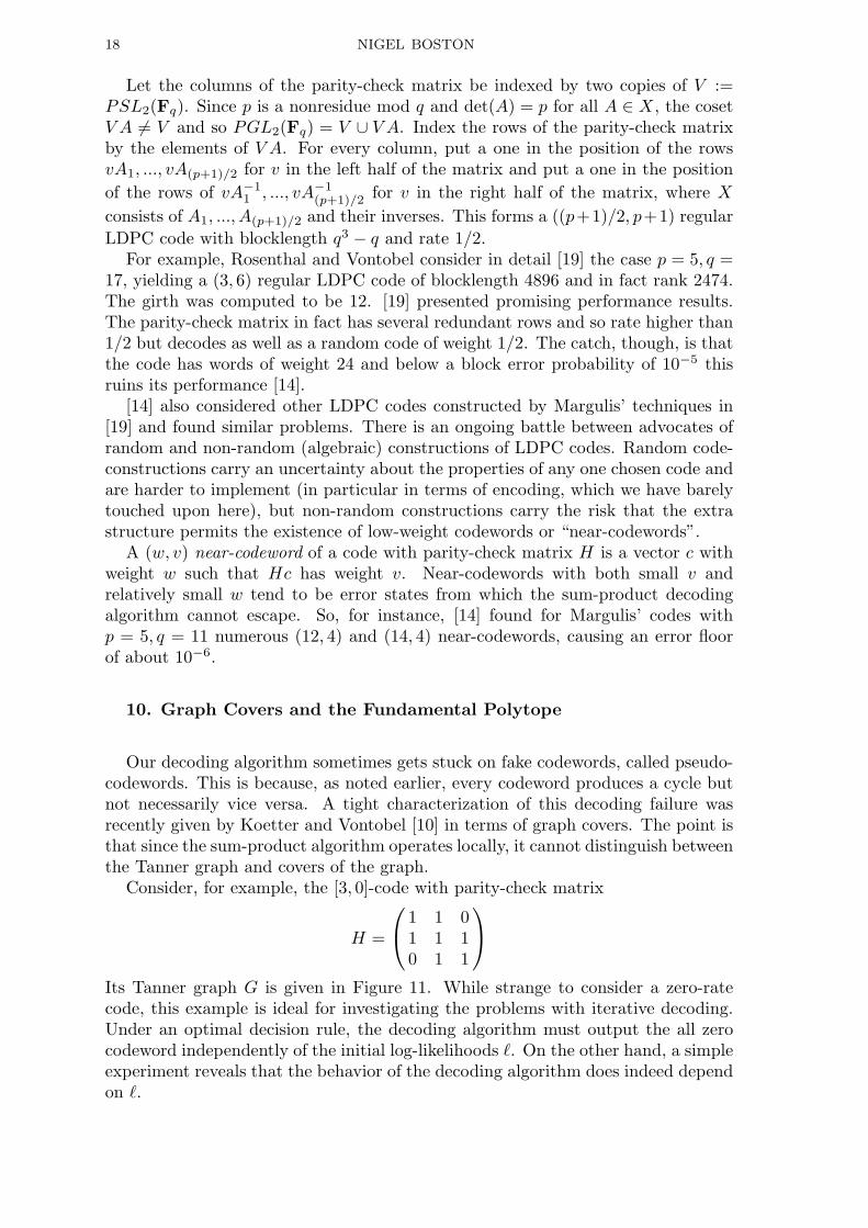
Let the columns of the parity-check matrix be indexed by two copies of V :=PSL2(Fq). Since p is a nonresidue mod q and det(A) = p for all A ∈ X, the cosetV A 6= V and so PGL2(Fq) = V ∪ V A. Index the rows of the parity-check matrixby the elements of V A. For every column, put a one in the position of the rowsvA1, ..., vA(p+1)/2 for v in the left half of the matrix and put a one in the positionof the rows of vA−1

1 , ..., vA−1(p+1)/2 for v in the right half of the matrix, where X

consists of A1, ..., A(p+1)/2 and their inverses. This forms a ((p+1)/2, p+1) regularLDPC code with blocklength q3 − q and rate 1/2.

For example, Rosenthal and Vontobel consider in detail [19] the case p = 5, q =17, yielding a (3, 6) regular LDPC code of blocklength 4896 and in fact rank 2474.The girth was computed to be 12. [19] presented promising performance results.The parity-check matrix in fact has several redundant rows and so rate higher than1/2 but decodes as well as a random code of weight 1/2. The catch, though, is thatthe code has words of weight 24 and below a block error probability of 10−5 thisruins its performance [14].

[14] also considered other LDPC codes constructed by Margulis’ techniques in[19] and found similar problems. There is an ongoing battle between advocates ofrandom and non-random (algebraic) constructions of LDPC codes. Random code-constructions carry an uncertainty about the properties of any one chosen code andare harder to implement (in particular in terms of encoding, which we have barelytouched upon here), but non-random constructions carry the risk that the extrastructure permits the existence of low-weight codewords or “near-codewords”.

A (w, v) near-codeword of a code with parity-check matrix H is a vector c withweight w such that Hc has weight v. Near-codewords with both small v andrelatively small w tend to be error states from which the sum-product decodingalgorithm cannot escape. So, for instance, [14] found for Margulis’ codes withp = 5, q = 11 numerous (12, 4) and (14, 4) near-codewords, causing an error floorof about 10−6.

10. Graph Covers and the Fundamental Polytope

Our decoding algorithm sometimes gets stuck on fake codewords, called pseudo-codewords. This is because, as noted earlier, every codeword produces a cycle butnot necessarily vice versa. A tight characterization of this decoding failure wasrecently given by Koetter and Vontobel [10] in terms of graph covers. The point isthat since the sum-product algorithm operates locally, it cannot distinguish betweenthe Tanner graph and covers of the graph.

Consider, for example, the [3, 0]-code with parity-check matrix

H =

1 1 01 1 10 1 1

Its Tanner graph G is given in Figure 11. While strange to consider a zero-ratecode, this example is ideal for investigating the problems with iterative decoding.Under an optimal decision rule, the decoding algorithm must output the all zerocodeword independently of the initial log-likelihoods `. On the other hand, a simpleexperiment reveals that the behavior of the decoding algorithm does indeed dependon `.

GRAPH-BASED CODES 19

Suppose y = y1y2y3 is received and let the initial log-likelihood at the threemessage nodes be `1, `2, `3 so that ` = (`1, `2, `3). Fixing `1 = 0.013, [10] foundthat as `2, `3 range from −5 to 5, for the region in Figure 12 the algorithm failed toconverge after 100 iterations. A closer experimental study showed that the regionof convergence to the zero word is described well by `1 + `2 + `3 ≥ 0.

Consider now Figure 13. This graph GH is a cubic cover of G. Every nodeof G is repeated three times and local adjacency relationships preserved. Also inFigure 13 is indicated a codeword for the cubic cover GH that does not arise on G.Any locally operating message-passing algorithm will take into account all possiblecodewords on all possible covers of G. The codeword in Figure 13 is “closer” to ythan the all zero codeword in a region that would correspond to a virtually presentall one codeword.

It seems a formidable task to characterize all possible codewords introducedby the union of all finite covers of any degree (whose number grows faster thanexponentially in the degree), but there is an elegant description, thanks to thefundamental polytope, which we now describe.

If G is a Tanner graph for a code C of length n, then a degree m cover G is aTanner graph of a code C of length mn. Any codeword in C lifts to a codeword inC and conversely, given a codeword c in C, we define

ωi(c) := |{j : ci,j = 1}|/m

and set ω(c) = (ω1(c), ..., ωn(c)).

Definition. A pseudo-codeword of C is any such ω(c) for any finite cover C ofC.

For instance, the codeword c in Figure 13 yields pseudo-codeword (2/3, 2/3, 2/3).

Theorem. Let a Tanner graph Gδ be given, consisting of a single parity-checknode of degree δ and δ variable nodes, and Cδ be the corresponding code. Let Pδ

denote the set of pseudo-codewords ω(c) taken over the union of all covers of Gδ ofall degrees. The closure of P is the polytope

Pδ = {ω ∈ Rn : ω = xPδ,x ∈ R2δ−1, 0 ≤ xi ≤ 1,

∑i

xi = 1}

where the 2δ−1 × δ matrix Pδ contains all binary even weight vectors of the form(∑m

i=1 ci)/m.Let a Tanner graph G have check nodes f1, ..., fr and message nodes c1, ..., cn.

Let P be the set of pseudo-codewords taken over the union of all covers of G of alldegrees. The closure of P is the polytope

P = {ω ∈ Rn : ωΓ(fi) ∈ Pδ(fi), 1 ≤ i ≤ r}

P is a convex body entirely inside the positive orthant, with one corner locatedat the origin. As an example of how this can be used, consider the (3, 5) regular

20 NIGEL BOSTON

LDPC code constructed in [26]. This is a very nice [155, 64, 20] binary linear code.Its parity-check matrix is 93×155 but because of redundant rows its rate is actuallyhigher than 1− 93/155, namely 64/155 = 0.4129. The underlying graph has girth8, which together with the relatively large minimum distance 20 (28 is the largestknown for a [155, 64]-code) makes it an outstanding candidate for iterative decod-ing. However, one easily finds a pseudo-codeword of small pseudo-weight and theautomorphism group of the graph then yields at least 155 pseudo-codewords of thispseudo-weight (an example of MacKay-Postol’s observation of the potential weak-nesses of non-random LDPC code constructions - see the last section). Thus thelarge minimum distance of the code itself is largely irrelevant for the performanceof iterative decoding.

A finer understanding of the suboptimal behavior of iterative decoding has inthe last few sections been attributed to stopping sets, near-codewords, and thefundamental polytope. How are these interrelated? While the notion of stoppingset is well-suited to the BEC, it does not work well with the AWGN channel. Whilethe notion of near-codewords helps understand potential problems in the designof iteratively decodable codes, it is not as refined a notion as the fundamentalpolytope. Any near-codeword can be completed into a pseudo-codeword, giving aprecise measure of the effect of the near-codeword.

BIBLIOGRAPHY

[1] S.M.Aji and R.J.McEliece, The generalized distributive law, IEEE Trans.Inform. Theory, 46, 325–343, 2000.

[2] L.R.Bahl, J.Cocke, F.Jelinek, and J.Raviv, Optimal decoding of linear codesfor minimizing symbol error rate, IEEE Trans. Inform. Theory, 20, 284–287, 1974.

[3] E.Berlekamp, R.McEliece, and H.van Tilborg, On the inherent intractabilityof certain coding problems, IEEE Trans. Inform. Theory, 24, 384–386, 1978.

[4] C.Berrou, A. Glavieux, and P.Thitimajshima, Near Shannon limit error-correcting coding and decoding, Proceedings of ICC ’93, 1064–1070, 1993.

[5] S.-Y.Chung, G.D.Forney, Jr., T.J.Richardson, and R.Urbanke, On the designof low-density parity-check codes within 0.0045 dB of the Shannon limit, IEEEComm. Letters, 5, 58–60, 2001.

[6] P.Elias, Coding for two noisy channels, Information Theory, 3rd LondonSymposium, 61–76, 1955.

[7] Flarion Technologies, Vector-LDPC Coding Solution,www.flarion.com/products/vector.asp[8] G.D.Forney, Jr., The Viterbi algorithm, Proc. IEEE, 61, 268–278, 1973.[9] R.G.Gallager, Low Density Parity-Check Codes, MIT Press, Cambridge, MA

1963.[10] R.Koetter and P.Vontobel, Graph-covers and iterative decoding of finite

length codes, Turbo conference, Brest, 2003.[11] M.Luby, M.Mitzenmacher, M.A.Shokrollahi, D.Spielman, and V.Stemann,

Practical loss-resilient codes, Proc. 29th Annual ACM Symposium on Theory ofComputing, 150–159, 1997.

[12] D.J.C.MacKay, Good error correcting codes based on very sparse matrices,IEEE Trans. Inform. Theory, 45, 399–431, 1999.

[13] D.J.C.MacKay, Gallager code resources,

GRAPH-BASED CODES 21

www.inference.phy.cam.ac.uk/mackay/CodesFiles.html[14] D.J.C.MacKay and M.S.Postol, Weaknesses of Margulis and Ramanujan-

Margulis low-density parity-check codes, Electronic Notes in Theoretical ComputerScience, 74, 2003.

[15] G.A.Margulis, Explicit constructions of graphs without short cycles and lowdensity codes, Combinatorica, 2, 71–78, 1982.

[16] J.Pearl, Probabilistic Reasoning in Intelligent Systems: Networks of Plausi-ble Inference, Morgan Kaufmann Publishers, Inc., 1988.

[17] T.Richardson, A.Shokrollahi, and R.Urbanke, Design of capacity-approachingirregular low-density parity-check codes, IEEE Trans. Inform. Theory, 47, 619–637,2001.

[18] T.Richardson and R.Urbanke, Modern Coding Theory, Lecture Notes,http://lthcwww.epfl.ch/papers/ics.ps[19] J.Rosenthal and P.Vontobel, Constructions of LDPC codes using Ramanu-

jan graphs and ideas from Margulis, Proc. 38th Annual Allerton Conference onCommunication, Control, and Computing, 248–257, 2000.

[20] I.Sason, Codes on graphs and iterative decoding algorithms,www.ee.technion.ac.il/people/sason/slides codes on graphs.pdf[21] C.E.Shannon, A Mathematical Theory of Communication, Bell System Tech-

nical Journal, vol. 27, 379–423, 1948 (Part I), 623–656 (Part II).[22] A.Shokrollahi, Codes and graphs, Proc. of STACS 2000, Lecture Notes in

Computer Science 1770, 1–12, 2000.[23] A.Shokrollahi, LDPC codes: an introduction,www.ipm.ac.ir/IPM/homepage/Amin2.pdf[24] M.Sipser and D.Spielman, Expander codes, IEEE Trans. Inform. Theory,

42, 1710–1722, 1996.[25] R.M.Tanner, A recursive approach to low complexity codes, IEEE Trans.

Inform. Theory, 27, 533–547, 1981.[26] R.M.Tanner, D.Sridhara, and T.Fuja, A class of group-structured LDPC

codes, Proc. of ICSTA 2001, Ambleside, England, 2001.[27] A.J.Viterbi, Error bounds for convolutional codes and an asymptotically

optimum decoding algorithm, IEEE Trans. Inform. Theory, IT-13, 260–269, 1967.[28] N.Wiberg, H.-A,Loeliger, and R.Koetter, Codes and iterative decoding on

general graphs, European Transactions in Telecommunication, 6, 513–525, 1995.[29] J.K.Wolf, A tutorial on low density parity check (LDPC) codes,ece-classweb.ucsd.edu/ece154c/LDPC.ppt, 2004.[30] V.V.Zyablov and M.S.Pinsker, Estimation of error-correction complexity of

Gallager low-density codes, Probl. Inform. Transm., 11, 18–28, 1976.

Departments of Mathematics, Electrical and Computer Engineering, and Com-

puter Sciences, University of Wisconsin, Madison, WI 53706, USAE-mail address: boston@math.wisc.edu