graphs in hlm. model setup, run the analysis before graphing sector = 0 public school sector = 1...
TRANSCRIPT

Graphs in HLM

Model setup, Run the analysis before graphing
• Sector = 0 public school• Sector = 1 private school

Graph entire model

With level 1 predictor

Here it is the graph
-3.76 -2.15 -0.53 1.08 2.694.29
7.87
11.45
15.03
18.61
SES
MA
TH
AC
H

Add level 2 categorical variable

And the graph
-3.76 -2.15 -0.53 1.08 2.691.05
5.79
10.53
15.27
20.01
SES
MA
TH
AC
H
SECTOR_M = 0
SECTOR_M = 1

Add level 2 continuous variable

What happened if we choose 25th and 75th percentiles?
-1.04 -0.52 -0.01 0.51 1.029.07
11.06
13.05
15.04
17.03
SES
MA
TH
AC
H
MEANSES = -0.296
MEANSES = 0.332

We can choose other options, say, 25th/50th/75th percentiles

The graph with 3 MEANSES levels
9.07
11.06
13.05
15.04
17.03
MA
TH
AC
H
-1.04 -0.52 -0.01 0.51 1.02
SES
MEANSES = -0.296
MEANSES = 0.037
MEANSES = 0.332

More complicated graph

More complicated graph
7.79
10.15
12.51
14.86
17.22
MA
TH
AC
H
-1.04 -0.52 -0.01 0.51 1.02
SES
MEANSES = -0.296,SECTOR_M = 0
MEANSES = -0.296,SECTOR_M = 1
MEANSES = 0.037,SECTOR_M = 0
MEANSES = 0.037,SECTOR_M = 1
MEANSES = 0.332,SECTOR_M = 0
MEANSES = 0.332,SECTOR_M = 1

Graph level 1 equation

The graph with first 10 groups (schools)
-1.66 -0.87 -0.07 0.72 1.514.36
8.82
13.29
17.75
22.21
SES
MA
TH
AC
H

What if we choose n=160 schools?
1.26
6.67
12.07
17.48
22.89
MA
TH
AC
H
-3.27 -1.66 -0.05 1.57
SES

With level 2 predictor: sector
-3.76 -2.15 -0.53 1.08 2.691.26
6.67
12.07
17.48
22.89
SES
MA
TH
AC
H
SECTOR_M = 0
SECTOR_M = 1

Add level 2 categorical variable

1.43
6.43
11.44
16.45
21.45
MA
TH
AC
H
-1.66 -0.68 0.30 1.27
SES
SECTOR_M = 0
SECTOR_M = 1

Add a level 2 continuous variable

1.26
5.55
9.83
14.12
18.40
MA
TH
AC
H
-1.66 -0.66 0.35 1.35
SES
MEANSES: lower
MEANSES: mid 50%
MEANSES: upper

Level 1 residual box-whisker
• To examine distributions of level-1 residuals.
• Normality assumption
• Homogeneity of variance

Level 1 residual box-whisker
-16.83
-8.19
0.45
9.09
17.73
Lev
el-1
Res
idu
al
0 3.00 6.00 9.00 12.00

Also could add a level 2 predictor
0 3.00 6.00 9.00 12.00-16.83
-8.19
0.45
9.09
17.73
Lev
el-1
Res
idu
al
SECTOR_M = 0
SECTOR_M = 1
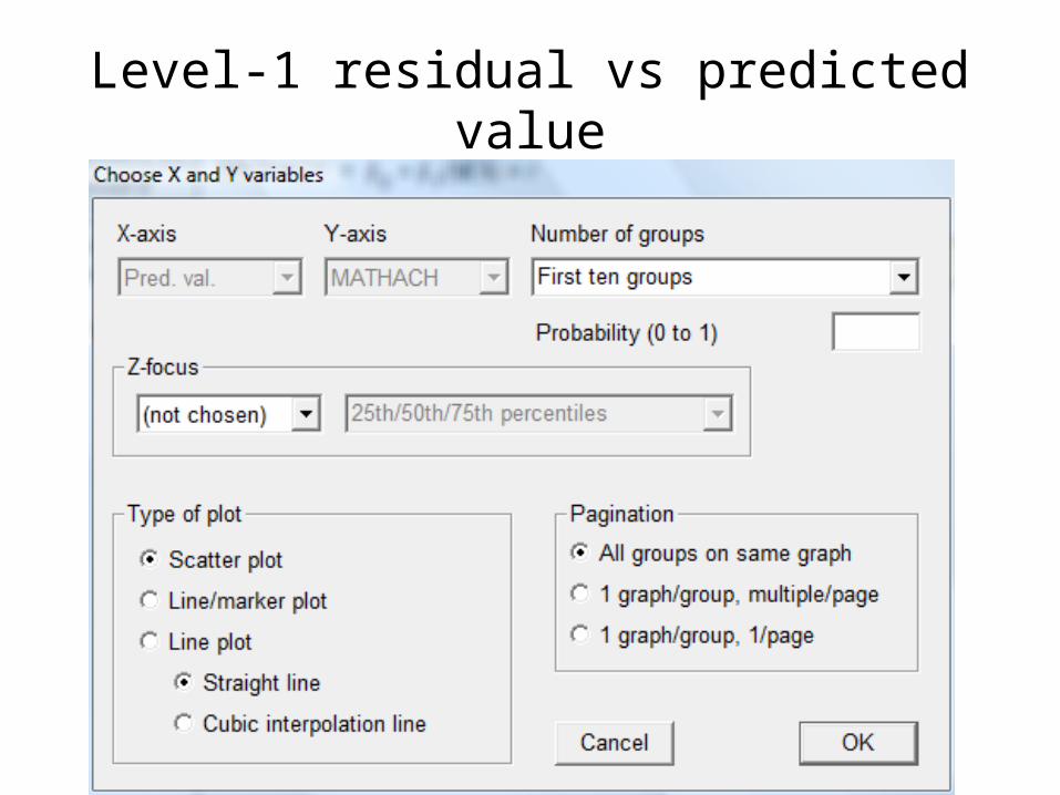
Level-1 residual vs predicted value

• Observe the pattern of residual scatter
Level-1 residual vs predicted value
5.35 9.18 13.01 16.83 20.66-15.30
-7.45
0.41
8.26
16.12
Level-1 Predicted Value
Lev
el-1
Res
idu
al

Add level 2 - sector
-15.30
-7.45
0.41
8.26
16.12
Lev
el-1
Res
idu
al
5.35 9.18 13.01 16.83 20.66
Level-1 Predicted Value
SECTOR_M = 0
SECTOR_M = 1

One graph per group, multiple graphs per page


Level-2 EB/OLS coefficient confidence intervals
• Compare the estimated empirical Bayes (EB) and OLS estimates of randomly varying level-1 coefficients (intercept and other coefficients).

Intercept with level 2 sectors
2.14
7.49
12.83
18.18
23.52
INT
ER
CE
PT
0 40.50 81.00 121.50 162.00
SECTOR_M = 0
SECTOR_M = 1

Intercept with level 2 MEANSES
2.14
7.49
12.83
18.18
23.52
INT
ER
CE
PT
0 40.50 81.00 121.50 162.00
MEANSES: lower
MEANSES: mid 50%
MEANSES: upper

Slope of SES

-0.01
1.15
2.31
3.47
4.63
SE
S
0 40.50 81.00 121.50 162.00
SECTOR_M = 0
SECTOR_M = 1

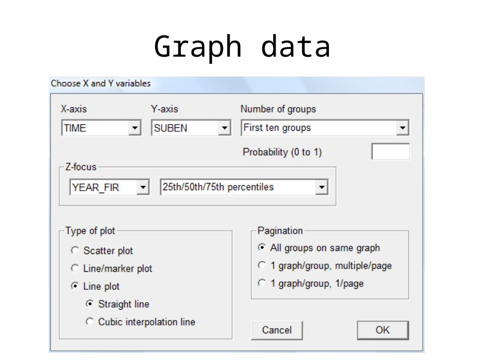
Graph data

Math regressed on SES (10 schools)
-1.82 -0.94 -0.07 0.80 1.67-4.22
3.43
11.08
18.73
26.38
SES
MA
TH
AC
H
SECTOR_M = 0
SECTOR_M = 1

One graph per group, multiple graphs per page

SECTOR_M = 0 SECTOR_M = 1

Longitudinal data

Whole model (CB- HLM Longitudinal Example)

235.5
243.6
251.8
259.9
268.0
SU
BE
N
0 4.61 9.22 13.82 18.43
TIME
GENDER_M = 1
GENDER_M = 2

With gender and year (level 2)
235.4
243.7
251.9
260.2
268.5
SU
BE
N
0 4.61 9.22 13.82 18.43
TIME
GENDER_M = 1,YEAR_FIR = 2
GENDER_M = 1,YEAR_FIR = 3
GENDER_M = 2,YEAR_FIR = 2
GENDER_M = 2,YEAR_FIR = 3
Graph data

178.9
212.2
245.5
278.8
312.1
SU
BE
N
-1.22 5.49 12.20 18.91 25.62
TIME
YEAR_FIR: lower
YEAR_FIR: mid 50%
YEAR_FIR: upper

