Gravity and Heterogeneous Trade Cost Elasticities¤y

Heterogeneous Trade Cost Elasticities

Natalie Chen Dennis Novy

April 16, 2021

Abstract

How do trade costs a¤ect international trade? This paper o¤ers a new approach. We rely

on a ‡exible gravity equation that predicts variable trade cost elasticities, both across and

within country pairs. We apply this framework to popular trade cost variables such as

currency unions, trade agreements, and WTO membership. While we estimate that these

variables are associated with increased bilateral trade on average, we …nd substantial

heterogeneity. Consistent with the predictions of our framework, trade cost e¤ects are

strong for ‘thin’ bilateral relationships characterised by small import shares, and weak or

even zero for ‘thick’ relationships.

JEL Classi…cation: F14, F15, F33.

Keywords: Currency Unions; Euro; Gravity; Heterogeneity; RTA; Trade Costs; Trade

Elasticity; Translog; WTO.

¤Natalie Chen, Department of Economics, University of Warwick, Coventry CV4 7AL, UK, CESifoand CEPR. E-mail: N.A.Chen@warwick.ac.uk (corresponding author), and Dennis Novy, Departmentof Economics, University of Warwick, Coventry CV4 7AL, UK, CEP/LSE, CESifo and CEPR. E-mail:D.Novy@warwick.ac.uk.

yThis paper was previously circulated as ‘Currency Unions, Trade, and Heterogeneity.’ We thank the editorNezih Guner and two anonymous referees for many valuable comments. We gratefully acknowledge …nancial sup-port from the Centre for Competitive Advantage in the Global Economy at the University of Warwick (CAGE,ESRC grant ES/L011719/1) and the Economic and Social Research Council (ESRC grant ES/P00766X/1).We are also grateful to Daniel Baumgarten, Douglas Campbell, Swati Dhingra, James Fenske, Boris Georgiev,Chris Meissner, John Morrow, Toshihiro Okubo, Andrew Rose, João Santos Silva, and to participants at theChina IEFS Conference 2017, the 13th Danish International Economics Workshop Aarhus 2017, the Royal Eco-nomic Society Conference Bristol 2017, the Society for International Trade Theory Conference Dublin 2017, theWorkshop on Public Economic Policy Responses to International Trade Consequences Munich 2017, the Tradeand Development Conference Hong Kong 2016, the Dynamics, Economic Growth, and International TradeConference Nottingham 2016, the RIETI Conference Tokyo 2016, the Delhi School of Economics, the EuropeanBank for Reconstruction and Development, the Paris Trade Seminar, Kiel, LSE, Middlesex, Nottingham, Oslo,Sussex, and to the CAGE and macro groups at Warwick.

1 Introduction

A key research topic in international trade is to understand the link between trade costs and

trade ‡ows. In this paper, we propose a new approach that is built on the idea that trade

costs may not a¤ect all trade ‡ows in the same way. Instead, trade costs might have a strong

in‡uence on trade between some countries but not between others.

To evaluate the e¤ect of trade costs, researchers typically rely on a standard gravity equation

framework and insert trade cost proxies as right-hand side regressors (e.g., bilateral distance,

dummy variables for regional trade agreements, currency union status, etc.) This yields single

coe¢cients to assess the trade e¤ects of these variables. By construction, their e¤ects are

homogeneous across all country pairs in the sample.1

In this paper, we challenge the view that trade costs have a homogeneous ‘one-size-…ts-all’

e¤ect on bilateral trade ‡ows. The core of our paper is to o¤er an easy-to-implement alternative

to the traditional gravity equation that allows us to estimate heterogeneous trade cost e¤ects.

Our contribution is to empirically demonstrate in a systematic and comprehensive way that

trade cost e¤ects are heterogeneous across country pairs, and also within country pairs by

direction of trade.

As a prominent example, consider the trade e¤ect of currency unions. Currency unions

are arguably an important institutional arrangement to reduce trade costs. In the period

since World War II, a total of 123 countries have been involved in a currency union at some

point. By the year 2015, 83 countries continued to do so. In addition, various countries are

currently considering to form new currency unions or to join existing ones.2 But does that

mean all currency union member pairs experience an equal increase in international trade? We

provide an empirical framework showing that the trade e¤ects associated with currency union

membership are heterogeneous across member pairs, even within speci…c currency unions such

as the euro.

We also apply this framework of ‡exible trade cost e¤ects to a host of other trade cost-related

variables popular in the international trade literature. We provide evidence of heterogeneous

e¤ects for regional trade agreements (RTAs), World Trade Organization (WTO) membership,

bilateral distance, sharing a common border, a common language, and tari¤s.

As our theoretical framework, we introduce heterogeneous trade cost e¤ects by taking guid-

ance from a translog gravity equation that predicts variable trade cost elasticities (Novy, 2013).

1To be precise, the direct (partial equilibrium) trade e¤ects are homogeneous. We discuss general equilibriume¤ects in Appendix B.

2Currency unions, or monetary unions, ‘are groups of countries that share a single money’ (Rose, 2006).See Data Appendix A for details. Areas currently considering the creation of a common currency include theeconomies of the West African Monetary Zone, the Southern African Development Community, the East AfricanCommunity, and the Gulf Cooperation Council (although in the latter case, talks have stalled).

2

In this framework, ‘thin’ bilateral trade relationships (characterised by small bilateral import

shares) are more sensitive to trade cost changes compared to ‘thick’ trade relationships (charac-

terised by large bilateral import shares). The intuition is that small import shares are high up

on the demand curve where sales are very sensitive to trade cost changes. Large import shares

are further down on the demand curve where sales are more bu¤ered. As a result, smaller

import shares have a larger trade cost elasticity in absolute magnitude. The prediction is that

a given change in trade costs (induced by a change in currency union status or other trade

cost changes) generates heterogeneous e¤ects on trade ‡ows. We should expect larger trade

e¤ects for country pairs associated with smaller import shares. This implies a heterogeneous

e¤ect even within country pairs since bilateral import shares typically di¤er depending on the

direction of trade.

We start by laying out the ‡exible gravity framework and relate it to trade cost e¤ects in

international trade. This forms the basis for our empirical speci…cations. We then construct

our key variable of interest – the bilateral import shares of 199 countries between 1949 and

2013 – and bring the framework to the data.3 We adopt two main approaches to test whether

the e¤ect of trade costs on trade is heterogeneous across import shares. The …rst approach

is a modi…cation of the standard gravity speci…cation familiar from the literature. Instead of

estimating a single trade cost coe¢cient that is constant over the entire sample, we propose a

‡exible gravity framework that allows for heterogeneous trade cost e¤ects across import shares.4

The second approach is to estimate the translog gravity equation directly, which also implies

variable trade cost elasticities.

In the …rst approach, our aim is to examine whether trade cost e¤ects are heterogeneous

across bilateral import shares. In principle, this could be attempted by interacting trade cost

regressors with import shares. However, this would create an immediate simultaneity bias

problem since trade cost e¤ects would vary with the values taken by the dependent variable.

We address this issue by letting trade cost e¤ects vary across predicted import shares. We

propose a two-step methodology for this purpose. In the …rst step we generate predicted shares

by regressing import shares on time-invariant geography-related variables such as distance and

contiguity. In the second step we assess how the trade cost e¤ects vary across predicted import

shares. To deal with heteroskedasticity and to include the zero import shares in the sample,

we estimate our regressions by Poisson Pseudo Maximum Likelihood (PPML), as is typical in

the recent gravity literature.

We carry out Monte Carlo simulations to verify the validity of our two-step procedure of

estimating heterogeneous trade cost e¤ects. When we assume that the data generating process

is driven by variable trade cost elasticities, we show that our two-step procedure produces

3As explained in Section 2, the dependent variable is actually the bilateral import share per good of theexporting country. But for simplicity we refer to it as the bilateral ‘import share.’

4It is well known that the gravity model …ts the data very well. The main point of adopting the ‡exiblegravity framework is not necessarily to improve overall …t but to introduce variable trade cost elasticities.

3

heterogeneous results that match those implied by the model, both qualitatively and quanti-

tatively. Also, when we assume that standard gravity with a constant trade cost elasticity is

the data generating process, we demonstrate that our two-step procedure does not spuriously

generate heterogeneous trade cost e¤ects.

To illustrate our procedure we initially focus on the e¤ect of currency unions on international

trade, and we turn to other trade cost variables later. Empirically, we …nd that when we

estimate a standard gravity regression without heterogeneous e¤ects (i.e., imposing a constant

trade cost elasticity), a common currency is associated with 29% more trade on average. Our

contribution with the help of the ‡exible gravity framework is to demonstrate that this average

hides a signi…cant amount of heterogeneity across country pairs. Bilateral trade e¤ects tend

to be particularly strong between countries where at least one partner is relatively small so

that import shares can be small. For example, we …nd a strong currency union e¤ect for trade

from Chad to Côte d’Ivoire (141% more bilateral trade) and from Austria to Germany (62%).

Conversely, bilateral trade e¤ects tend to be relatively weak or even zero between countries

with large import shares, for example from Côte d’Ivoire to Togo (22%) and from France to

Belgium-Luxembourg (insigni…cant).

We also …nd that the trade e¤ect of currency unions is heterogeneous within country pairs

and therefore asymmetric by direction of trade. For example, as just mentioned, the e¤ect

is large (62%) for trade from Austria to Germany (a low bilateral import share). But it is

insigni…cant for trade from Germany to Austria (a large bilateral import share).

Given the enormous academic and policy interest in the euro, we also focus more speci…cally

on the trade e¤ect of the European single currency. Consistent with evidence reported in the

literature, we con…rm that the average trade e¤ect of the euro is more modest compared to

other common currencies.5 This is consistent with relatively large import shares on average in

the euro area. Still, we …nd that the e¤ect is heterogeneous across country pairs within the

Eurozone. Examples of country pairs with small import shares which are associated with large

euro e¤ects include Ireland importing from Cyprus (70%) and Finland importing from Malta

(50%). Conversely, country pairs with large import shares not generating any additional trade

from the common currency include Cyprus importing from Greece and Germany importing

from Italy.

Recent contributions show that estimating a gravity equation by PPML as opposed to

log-linear Ordinary Least Squares (OLS) reduces the size and signi…cance of the estimated

trade e¤ect of currency unions, and in particular of the euro.6 Our framework contributes to

explaining this …nding. As is well known, OLS and PPML estimators have di¤erent …rst-order

5See Micco et al. (2003), Baldwin (2006), Baldwin and Taglioni (2007), Baldwin et al. (2008), Berger andNitsch (2008), Santos Silva and Tenreyro (2010), Eicher and Henn (2011), Glick and Rose (2016), Mika andZymek (2018), Larch et al. (2019), Mayer et al. (2019), or Campbell and Chentsov (2020).

6For instance, Santos Silva and Tenreyro (2010), Mika and Zymek (2018), Larch et al. (2019), and Mayeret al. (2019) …nd that PPML estimates of the euro trade e¤ect are insigni…cant.

4

conditions (Eaton et al., 2013; Head and Mayer, 2014; Mayer et al., 2019). While the OLS

conditions involve logarithmic deviations of trade from its expected value, the PPML conditions

involve level deviations and therefore tend to give more weight to country pairs with high levels

of trade. By highlighting that country pairs with higher trade intensity have a smaller trade

cost elasticity, our framework therefore predicts that the PPML currency union estimate should

be smaller than its OLS counterpart.

In the second approach, we explore the predictions of our model by estimating the translog

gravity equation directly. Our regressions con…rm that a common currency is associated with

more bilateral trade, and that the magnitude of the e¤ect falls with bilateral import shares.

One concern about our estimations relates to the potentially endogenous nature of trade cost

variables. For example, reverse causality may arise because countries that trade intensively with

each other are more likely to join a currency union, leading to an overestimation of the trade

e¤ect of common currencies.7 Attempts in the literature to instrument the currency union

dummy variable prove disappointing as the instrumentation tends to increase, rather than

decrease, the magnitude of currency union estimates (Rose, 2000; Alesina et al., 2002; Barro

and Tenreyro, 2007). This has led the profession to conclude that appropriate instruments for

currency union membership are not available (see Baldwin, 2006, for a discussion).

In this paper, we do not attempt to instrument the currency union indicator. But in

simulation results we show that correcting for endogeneity bias (to the extent that it exists)

should strengthen, rather than weaken, the heterogeneity patterns in our results. The intuition

is that bilateral trade and currency unions are positively related. This would result in positive

endogeneity bias, pushing up the modest currency union e¤ects associated with large import

shares. Thus, removing this potential bias would lead to even stronger heterogeneity patterns.

Endogeneity can therefore not overturn our heterogeneity results.

As they improve our understanding of how trade costs shape trade ‡ows between trading

partners, our results have important policy implications. Most importantly, they help to eval-

uate the potential changes in bilateral trade ‡ows that countries can expect when their trade

costs change. For instance, suppose Bulgaria, Croatia, the Czech Republic, Hungary, Poland,

Romania, and Sweden were to join the euro over the next few years. As these countries are

relatively small compared to some members of the Eurozone such as France and Germany, they

have relatively large import shares. Our results suggest that these import shares will grow only

modestly (Baldwin, 2006; Glick, 2017; Mika and Zymek, 2018). However, trade shares in the

opposite direction are smaller and can therefore be expected to grow more strongly.

7Trading …rms hurt by exchange rate ‡uctuations may lobby to keep the exchange rate with the country’smajor trading partners …xed (Baldwin, 2006). Reverse causality could also arise if currency unions captureunobserved characteristics that a¤ect trade ‡ows. For evidence that greater bilateral trade reduces bilateralexchange rate volatility, see Devereux and Lane (2003) and Broda and Romalis (2010). Mundell (1961) suggeststhat by reducing real exchange rate ‡uctuations, trade reduces the costs of forming a currency union. Alesinaand Barro (2002) show that countries trading more with each other are more likely to form currency unions.

5

Our approach is by no means the only one to explore heterogeneous trade cost elasticities.

Novy (2013) concentrates on the theoretical derivation of the translog gravity framework, and

he only explores its empirical implications based on bilateral distance and contiguity using

a single cross-section of 28 OECD countries with fewer than a thousand observations. By

contrast, we use more than 1.1 million observations and explore the empirical importance of

heterogeneous trade cost e¤ects in a more comprehensive way using a broad range of trade

cost variables popular in the literature including time-varying components such as currency

union status, regional trade agreements, and WTO membership. Bas et al. (2017) derive

country pair aggregate trade cost elasticities from a monopolistic competition model with CES

demand and log-normal …rm-level heterogeneity. Consistent with our predictions, they …nd that

the trade cost elasticity is smaller in magnitude for country pairs with large trade volumes.

Guided by monopolistic competition models with CES demand and truncated Pareto …rm-level

productivity, Helpman et al. (2008) …nd that bilateral trade cost elasticities are larger for less

developed countries, while Melitz and Redding (2015) document that those elasticities vary

across markets and levels of trade costs. Spearot (2013) relies on the Melitz and Ottaviano

(2008) model with …rm-level heterogeneity and linear demand to show that tari¤ liberalisation

disproportionately increases the imports of low revenue varieties. Carrère et al. (2020) also

stress the importance of non-constant trade elasticities, focusing on the e¤ect of distance in

particular.8

More speci…cally, our paper also contributes to a large and growing literature that explores

whether currency unions promote trade. In his seminal work, Rose (2000) shows that sharing

a common currency more than triples bilateral trade ‡ows. Subsequent work by Rose and

co-authors shows that the currency union e¤ect is smaller than initially found but remains

large (Rose and van Wincoop, 2001; Frankel and Rose, 2002; Glick and Rose, 2002). Various

authors argue that these …ndings are plagued by omitted variables, econometric errors, and self-

selection, may be driven by currency unions between small or poor countries, and that the trade

e¤ect of currency unions is small or insigni…cant.9 We rely on state-of-the-art PPML techniques

which allow us to include zero trade observations in the sample and control for country pair

and time-varying exporter and importer …xed e¤ects. In addition, our results remain robust

to endogeneity, self-selection, omitted variables such as wars and political con‡icts, and to

excluding small and poor countries as well as post-Soviet states from the sample.

Nevertheless, there is empirical evidence to suggest that heterogeneity in the trade impact

8Also see Atkeson and Burstein (2008) who derive heterogeneous trade cost elasticities from a model withnested CES demand and oligopolistic competition.

9See Persson (2001), Nitsch (2002), De Nardis and Vicarelli (2003), López-Córdova and Meissner (2003),Micco et al. (2003), Klein (2005), Baldwin (2006), Klein and Shambaugh (2006), Bun and Klaassen (2007),Baldwin et al. (2008), Berger and Nitsch (2008), Broda and Romalis (2010), Frankel (2010), Santos Silva andTenreyro (2010), Eicher and Henn (2011), De Sousa (2012), Campbell (2013), Glick and Rose (2016), Glick(2017), Saia (2017), Mika and Zymek (2018), Larch et al. (2019), and Campbell and Chentsov (2020). Baldwinet al. (2008) claim that the empirical literature on the trade e¤ect of currency unions ‘is a disaster’ as theestimates range from 0% (e.g., Berger and Nitsch, 2008) to 1,387% (Alesina et al., 2002), most of them being‘fatally ‡awed by misspeci…cation and/or econometric errors.’

6

of currency unions exists along several dimensions.10 For instance, the e¤ect is larger for

developing economies (Santos Silva and Tenreyro, 2010), smaller countries (Micco et al., 2003;

Baldwin, 2006), and falls over time (De Sousa, 2012). The e¤ect also varies across currency

unions (Nitsch, 2002; Klein, 2005; Eicher and Henn, 2011; Glick and Rose, 2016). Consensus

estimates for the euro tend to be more modest than those for broader samples, falling between

5% and 15% (Baldwin, 2006; Baldwin et al., 2008). The trade e¤ect is stronger for industries

producing di¤erentiated goods (Flam and Nordström, 2007), and for larger and more productive

…rms that adjust both at the intensive and extensive margins (Berthou and Fontagné, 2008).

In contrast to these papers where the various sources of heterogeneity are explored without

theoretical motivation and often across di¤erent samples, we are guided by a gravity framework

with ‡exible trade cost elasticities to derive our empirical speci…cations.

The remainder of the paper is organised as follows. In Section 2 we build on the translog

gravity framework to motivate why we might …nd heterogeneous trade cost e¤ects in the data.

In Section 3 we present our main estimation results. When introducing our empirical method-

ology, we initially focus on currency unions as a well-known trade cost variable to demonstrate

the heterogeneity of trade e¤ects. Then in Section 4 we extend the heterogeneity analysis to

other prominent trade cost variables popular in the gravity literature such as RTAs, WTO

membership, tari¤s, bilateral distance, and a shared border and language between trading

partners. In Section 5 we carry out Monte Carlo simulations that explore the endogeneity of

currency unions. In Section 6 we summarise an extensive battery of robustness checks. We

conclude in Section 7. Appendix A summarises our data and sources. In Appendix B we out-

line the derivation of the translog gravity equation. We also carry out Monte Carlo simulations

that validate our estimation strategy, and we discuss general equilibrium e¤ects. Appendix C

provides details on the robustness checks.

2 Theoretical Motivation

The conventional gravity framework in the literature is characterised by a constant trade cost

elasticity. This means that the direct e¤ect of a trade cost change is common across country

pairs.11 In this paper, we employ a gravity framework that does not feature a constant trade

cost elasticity. Instead, we build on a gravity framework with variable trade cost elasticities.

It follows that the e¤ect of a trade cost change is no longer common across country pairs. It

becomes heterogeneous.

As a framework that accommodates the crucial feature of variable trade cost elasticities, we

10On the heterogeneous trade e¤ects of FTAs, see Glick (2017) and Baier et al. (2019). Spearot (2013)studies the heterogeneous trade e¤ects of tari¤ liberalisation. Subramanian and Wei (2007) and Felbermayr etal. (2020) explore the heterogeneous trade e¤ects of WTO membership. Mayer et al. (2019) …nd that the tradee¤ects of belonging to the EU are heterogeneous across member states, and the countries gaining the most aresmall, open, and centrally located.

11See Head and Mayer (2014) for an overview.

7

use translog gravity to motivate our analysis. As in Novy (2013), the model features multiple

countries in general equilibrium that are endowed with an arbitrary number of di¤erentiated

goods. Demand is derived from a translog expenditure function using the parameterisation in

Feenstra (2003). Trade costs follow the iceberg form where tij ¸ 1 denotes the bilateral trade

cost factor between countries i and j. Trade costs may be bilaterally asymmetric such that

tij 6= tji.

As outlined in Appendix B.1, imposing market clearing and solving for the general equilib-

rium results in the translog gravity equation:

xij/yjni

= ¡θ ln(tij) +Di + θ ln(Tj), (1)

where xij is the bilateral trade ‡ow between exporting country i and importing country j, yjis the importer’s income, and ni denotes the number of goods of country i (we ignore time

indices for now). The dependent variable is the bilateral import share xij/yj per good ni of

the exporting country. On the right-hand side, θ > 0 is a translog preference parameter. Di

and Tj denote exporter and importer-speci…c terms given by:

Di =yi/y

W

ni+ θ

SX

s=1

ysyW

ln

µtisTs

¶

, (2)

ln (Tj) =SX

s=1

nsNln(tsj), (3)

where yW denotes world income, S is the number of countries, and N is the number of products

in the world with N ¸ S. Tj is akin to a multilateral resistance term since it represents a

weighted average of bilateral trade costs.

The translog gravity equation (1) di¤ers in two key respects from standard gravity equations

as in Eaton and Kortum (2002) and Anderson and van Wincoop (2003). The dependent variable

is the import share per good, which means an empirical measure of ni is required. In addition,

the dependent variable is in levels. It is not the logarithmic bilateral trade ‡ow. The gravity

relationship is therefore not log-linear in trade costs. This implies a variable trade cost elasticity.

This is the crucial feature we focus on in this paper.

More speci…cally, de…ne the trade cost elasticity as η ´ ∂ ln (xij) /∂ ln(tij). This is meant

as the direct trade cost elasticity in the sense that indirect general equilibrium price e¤ects

are omitted here (we discuss those general equilibrium e¤ects in detail in Appendix B.4). In

standard gravity equations this elasticity would be constant.12 In the translog gravity model,

12For instance, in Anderson and van Wincoop (2003) the elasticity would be equal to 1 ¡ σ where σ is theCES elasticity of substitution. In Eaton and Kortum (2002) it would be equal to the Fréchet shape parameter.In Chaney (2008) it would be equal to the Pareto shape parameter.

8

however, this elasticity is variable. It follows from equation (1) as:

ηij = ¡θ

xij/yjni

. (4)

That is, the trade cost elasticity is the preference parameter θ divided by the import share

per good. Therefore, the larger a given import share, the smaller the trade cost elasticity in

absolute magnitude. The ij subscript indicates that this elasticity varies by country pair.

In line with the literature, we assume that logarithmic trade costs ln(tij) are a function

of commonplace trade cost variables such as logarithmic bilateral distance, dummy variables

for contiguity, common language as well as membership of trade agreements, currency unions,

and so on. As an example, let us consider a dummy variable for currency union membership

CUij which takes on the value of one if countries i and j are both members, with coe¢cient

κ. We expect κ to be negative since a currency union is generally thought to lower bilateral

trade costs (our empirical results will con…rm this). Based on the expression in equation (4),

the e¤ect of currency union membership on trade follows as:

¢ln(xij)

¢CUij

¼ ¡θκ

xij/yjni

, (5)

where ¢CUij indicates entry into a currency union. Given that κ is likely negative, we expect

a positive currency union e¤ect on bilateral trade.

We would like to highlight a key aspect of our framework. As the denominators of expres-

sions (4) and (5) show, the heterogeneity of currency union e¤ects is driven by variation across

import shares. It would be conceivable that heterogeneity is instead driven by the currency

union parameter in the trade cost function, perhaps because di¤erent currency unions have

di¤erent trade cost e¤ects.13 However, as we show below in our empirical analysis, we …nd het-

erogeneous e¤ects across di¤erent pairs within a given currency union, and even within a given

bilateral country pair by direction of trade (due to bilaterally asymmetric import shares). This

means that even if trade costs are bilaterally symmetric, trade cost e¤ects can be bilaterally

asymmetric in the translog gravity framework.14

In summary, the most important insight from this motivating framework is the variable

trade cost e¤ect in expression (4). Speci…cally, the trade cost e¤ect should be larger in absolute

magnitude for country pairs associated with smaller import shares. It also follows that a

symmetric reduction in bilateral trade costs can lead to asymmetric increases in bilateral trade

‡ows by direction of trade. These are testable predictions we will now examine. While we

13Instead of the constant κ we would then have to adopt currency union-speci…c trade cost parameters. Weallow for such an approach in our analysis of the euro in Section 3.1.4.

14Trade ‡ows can also be bilaterally asymmetric, but trade is balanced at the aggregate country level due tothe general equilibrium nature of the model.

9

also estimate the translog speci…cation in equation (1) directly, we will …rst turn towards an

alternative approach.

3 Empirical Analysis

Our aim is to …nd out whether international trade data are characterised by variable trade cost

elasticities. As a starting point, we …rst estimate gravity regressions with a standard constant

trade cost elasticity. We then proceed by exploring variable trade cost elasticities. For that

purpose, we adopt two approaches that are consistent with the theoretical framework in Section

2. The …rst approach is a modi…cation of the standard gravity speci…cation commonplace in

the literature. Instead of estimating a single trade cost coe¢cient that is constant over the

entire sample, we propose a ‡exible gravity framework that allows for heterogeneous trade cost

e¤ects across import shares. We explain this estimating strategy in more detail below (see

Section 3.1). The second approach is to estimate the translog gravity equation (1) directly (see

Section 3.2).

We introduce our approach with an application to the trade e¤ect of currency unions. This

is mainly for expositional purposes, and later in the paper we extend the analysis to other

trade cost variables (see Section 4 in particular). We use a very large, comprehensive data set

of aggregate annual bilateral trade ‡ows that covers most of global trade in modern times. It

consists of an unbalanced panel including 199 countries from 1949 to 2013. We provide details

and descriptive statistics in Appendix A.

3.1 Gravity with Heterogeneity

This section describes our …rst approach. Focusing on currency unions, we start by estimating

homogeneous trade cost e¤ects with constant trade cost elasticities as in the standard gravity

framework. We then modify the gravity speci…cation and introduce a two-step procedure to

allow for trade cost heterogeneity. We also explore the trade e¤ect of the euro in more detail.

3.1.1 Homogeneous Trade Cost E¤ects in Standard Gravity

As pointed out by Santos Silva and Tenreyro (2006), the validity of estimating a log-linear

gravity model by OLS depends crucially on the assumption that the variance of the error

term is independent from the regressors. Otherwise, the log transformation prevents the error

term from having a zero conditional expectation, leading to inconsistent estimates of the true

elasticities. PPML instead delivers consistent coe¢cient estimates, even in the presence of

heteroskedasticity (Head and Mayer, 2014). Another advantage of PPML is that by expressing

the dependent variable in levels, zero trade observations can be incorporated in the estimation

(the log-linear gravity equation may su¤er from selection bias as the zero values drop out of

10

the regression). In our sample, around 35% of import shares are equal to zero (see Appendix

A). In what follows we therefore estimate our regressions by PPML.15

We initially estimate homogeneous trade cost e¤ects with a constant elasticity as in the

standard gravity framework, based on PPML regressions. But we use the bilateral import

share per good as the dependent variable to make sure our results are comparable to subsequent

estimates that allow for heterogeneous trade cost e¤ects. We thus estimate:

µxij,t/yj,tni,t

¶

= exp (α1CUij,t + α2Zij,t +Di,t +Dj,t +Dij) + ij,t, (6)

where we add time subscripts such that xij,t is the bilateral FOB export value from exporter i

to importer j in year t, yj,t is country j’s nominal GDP (both in US dollars), and ni,t denotes

the number of goods in the exporting country which can be interpreted as an extensive margin

measure. Trade costs depend on currency union membership CUij,t which is a dummy variable

taking on a value of one if countries i and j are both members in year t (and zero otherwise).

Trade costs are also a function of other time-varying country pair variables Zij,t which include

dummy variables equal to one if both countries in the pair belong to an RTA or are members

of the WTO, OECD, and IMF in each year, and zero otherwise (Rose, 2005). We return to

those other trade cost variables in Section 4.

To measure the exporting countries’ extensive margin ni,t we collect each country’s total

exports by product category from United Nations Comtrade which are available from 1962

onwards. As the HS classi…cation was only introduced in 1988, we rely on data at the 4-digit

HS level between 1988 and 2013, and at the 4-digit SITC level from 1962 to 1987. We de…ne

the extensive margin as the number of di¤erent product categories exported by each country

in each year relative to the total number of categories exported by all countries in the same

year. Given that the Comtrade data are only available from 1962, have poor country coverage

in some years, and are reported according to two di¤erent classi…cations over time (i.e., SITC

versus HS), we calculate the average extensive margin by exporter. This yields a time-invariant

measure ni but we believe that this measure should provide us with useful information regarding

the variation in the extensive margin across exporting countries.16

We later check the robustness of our …ndings by using an alternative proxy for the extensive

margin (see Table C5 in Appendix C). We rely on the cross-country measure constructed

15We employ the ppmlhdfe Stata command written by Correia et al. (2020). It estimates a Poisson PseudoMaximum Likelihood regression allowing for multiple levels of …xed e¤ects. In the previous version of ourpaper (Chen and Novy, 2018) results were based on OLS estimation. Those results are generally the samequalitatively, although individual magnitudes may be di¤erent between PPML and OLS.

16For each year from 1962 to 1987 we calculate the number of 4-digit SITC-level product categories exportedby each country relative to the total number of 4-digit SITC-level categories exported by all countries. For theyears 1988 to 2013 we do the same at the 4-digit HS level. For each country the time-invariant ni measure(that we use for our full sample between 1949 and 2013) is given by the average of the two series between 1962and 2013.

11

by Hummels and Klenow (2005) using data on exports from 126 exporting to 59 importing

countries in more than 5,000 6-digit HS-level product categories in 1995. We also assume that

the extensive margin is unity for all exporters, in which case the dependent variable is simply

the bilateral import share.

We control for an extensive set of …xed e¤ects. We include time-varying exporter and

importer …xed e¤ects Di,t andDj,t to control for multilateral trade resistance and other exporter

and importer-speci…c terms such as income. We also include country pair …xed e¤ects Dij to

absorb all time-invariant bilateral trade frictions in each cross-section. The country pair e¤ects

also help to control for the endogeneity of the currency union dummy if two countries deciding

to join a currency union have traditionally traded a lot with each other (but the pair e¤ects

fail to do so if the two countries join following a surge in trade during the sample period, see

Micco et al., 2003, or Bun and Klaassen, 2007). Note that the pair e¤ects are directional as

non-directional pair e¤ects would not capture the asymmetry in bilateral import shares within

a pair. Identi…cation is therefore achieved from the time series variation of each explanatory

variable within a pair (e.g., from changes in bilateral currency union status over time).17 To

control for time-invariant idiosyncratic shocks correlated at the pair level (De Sousa, 2012),

standard errors are clustered at the non-directional country pair level. The coe¢cients to be

estimated are denoted by the α’s. As sharing a common currency should be associated with

more trade, we expect α1 to be positive. The error term is ij,t.

3.1.2 Heterogeneous Trade Cost E¤ects

We then focus on trade cost heterogeneity. Our aim is to investigate whether the trade e¤ect of

currency unions, as captured by α1 in speci…cation (6), is heterogeneous across bilateral import

shares per good, as predicted by the theoretical framework in Section 2. If we simply allowed

α1 to vary with import shares, we would have a simultaneity bias problem as the currency

union e¤ect would vary with the values taken by the dependent variable (Novy, 2013).

To address this issue we modify the standard gravity speci…cation by letting the currency

union e¤ect vary across predicted import shares. For that purpose, we propose a two-step

methodology. In the …rst step we regress the import shares per good on geography-related

variables (distance and contiguity) to generate the predicted shares. In the second step we

investigate how the trade e¤ect of currency unions varies across predicted shares. We now

explain this approach in more detail.

In the …rst step we regress the import shares per good on time-invariant country pair

17Baier et al. (2019) use directional pair e¤ects to estimate the within-pair asymmetric e¤ects of FTAs. Therecent literature concludes that time-varying exporter and importer dummies and time-invariant country pair…xed e¤ects should be included (De Nardis and Vicarelli, 2003; Baldwin, 2006; Baldwin and Taglioni, 2007;Baldwin et al., 2008; Eicher and Henn, 2011; Mika and Zymek, 2018; Campbell and Chentsov, 2020). Theearlier literature failed to do so (e.g., Rose, 2000).

12

controls and exporter-year and importer-year …xed e¤ects:

µxij,t/yj,tni,t

¶

= exp (δKij +Di,t +Dj,t) + νij,t, (7)

where Kij includes geography-related variables, i.e., logarithmic bilateral distance and a conti-

guity dummy.18 We do not include the time-varying pair variables for currency unions, RTAs,

the WTO, OECD, or IMF as they are not geography-related and therefore more likely endoge-

nous. We then generate the predicted shares which we denote byd³

xij,t/yj,tni,t

´.

In the second step we include an interaction term between the currency union dummy

variable and the logarithmic predicted import shares, with ξ2 as the key coe¢cient of interest.19

We estimate:

µxij,t/yj,tni,t

¶

= exp

Ã

ξ1CUij,t + ξ2CUij,t £ lndµ

xij,t/yj,tni,t

¶

+ ξ3Zij,t +Di,t +Dj,t +Dij

!

+ εij,t.

(8)

Since this speci…cation includes exporter-year, importer-year, and country pair …xed e¤ects,

the main e¤ect of the logarithmic predicted import share drops out of the regression. The

trade e¤ect of currency unions is given by ξ1 + ξ2 lnd³

xij,t/yj,tni,t

´and therefore depends on two

components, i.e., the change in trade costs due to currency unions and the log predicted import

share. If the trade e¤ect of currency unions falls with bilateral import intensity as predicted by

our theoretical framework, the interaction coe¢cient ξ2 should be negative. As the log predicted

import share is a generated regressor, we bootstrap standard errors with 100 replications.

The intuition of this two-step methodology is as follows. To avoid the simultaneity problem,

the predicted import shares generated in the …rst step should not be correlated with the error

term εij,t in the second step. The point of the …rst step is therefore to extract the exogenous

component of import shares. We aim to achieve this by using geography-related regressors

(distance and contiguity) as well as time-varying exporter and importer-speci…c …xed e¤ects,

and then predicting the import shares. In Appendix B we carry out Monte Carlo simulations to

verify the validity of this two-step procedure. In Section 5 we explore the potential endogeneity

of currency unions and reverse causality.

An alternative way of testing our prediction of heterogeneous currency union e¤ects is to

split the sample into intervals of predicted import shares per good ranked by value and to

18Our results remain robust if in the …rst-step regression (7) we allow for time-varying distance and contiguitycoe¢cients, include further gravity variables or simply control for time-invariant (directional) country pair …xede¤ects (see Section 6). They also remain robust if we add the currency union, RTA, WTO, OECD, and IMFvariables.

19We interact with the logarithmic share since the dependent variable and the interaction term are thenexpressed in the same units, i.e., they are expressed as level shares if we exponentiate the logarithmic share onthe right-hand side of equation (8).

13

estimate:µxij,t/yj,tni,t

¶

= exp¡β1,hCUij,t £ Dh + β2Zij,t +Di,t +Dj,t +Dij +Dh

¢+ ij,t, (9)

where Dh is a dummy variable for h equally-sized intervals of predicted import shares per good.

The currency union coe¢cient β1,h is estimated separately for each interval h. Consistent with

our theoretical framework, we expect the currency union e¤ect to be largest in the interval of

lowest predicted shares, and to be weaker in intervals of higher shares.20

3.1.3 Baseline Results

We start by discussing homogeneous currency union estimates. Before turning to PPML es-

timation, in column (1) of Table 1 we …rst estimate the log-linear version of equation (6) by

OLS, using the log bilateral import share per good as the dependent variable (the zero observa-

tions therefore drop out from the regression). The currency union coe¢cient is equal to 0.326,

suggesting that a common currency is associated with an increase in bilateral trade of 39% on

average (exp (0.326) ¡ 1 = 0.385). We note that this currency union estimate captures direct

trade cost e¤ects.21 Joining an RTA, and becoming a member of the WTO, OECD, and IMF

are associated with an increase in bilateral trade (Rose, 2005).

Next, we regress equation (6) by PPML but we omit the zero observations from the sample.

This allows us to assess how PPML a¤ects coe¢cient estimates. As explained by Mayer et

al. (2019), OLS and PPML estimates may di¤er because the two estimators have di¤erent

…rst-order conditions (Eaton et al., 2013; Head and Mayer, 2014). While the OLS conditions

involve logarithmic deviations of trade from its expected value, the PPML conditions involve

level deviations and therefore tend to give more weight to country pairs with high levels of

trade.22 If country pairs with higher import intensity have smaller trade cost elasticities, as we

argue, then the PPML currency union coe¢cient should be smaller than its OLS counterpart.

In column (2) the currency union estimate decreases to 0.202 such that sharing a common

currency is associated with 22% more trade on average. This result is therefore consistent with

20Quantile regressions could also be used to test our predictions. Various …xed e¤ect estimators have recentlybeen developed but little is known about their performance. Using the qreg2 Stata command of Parenteand Santos Silva (2016), we instead estimated pooled quantile regressions with clustered standard errors. Thecurrency union e¤ect is overestimated due to the omission of the …xed e¤ects but we …nd that it falls withbilateral import shares.

21We discuss indirect general equilibrium e¤ects in Appendix B.4. Those are second-order e¤ects that arequantitatively small. The intuition is that currency unions are relatively rare at the bilateral level (see DataAppendix A), and they are only one out of several trade cost components. We also show that the generalequilibrium e¤ects are not systematically related to the heterogeneity of currency union e¤ects.

22To illustrate that PPML gives more weight to the country pairs with high levels of trade, Mayer et al.(2019) follow the approach of Eaton et al. (2013) who estimate a multinomial gravity model for aggregatebilateral trade shares. They regress the trade share (bilateral trade divided by total trade) by PPML, and astrade shares give less weight to the large trade ‡ows in levels they …nd that the coe¢cient estimates lie betweenthe OLS and PPML estimates of regressing bilateral trade ‡ows.

14

our prediction of country pairs with higher import shares having a smaller trade cost elasticity.23

It is also consistent with papers …nding that PPML reduces the size and signi…cance of currency

union estimates (Santos Silva and Tenreyro, 2010; Mika and Zymek, 2018; Larch et al., 2019;

Mayer et al., 2019). The WTO estimate becomes insigni…cant, while the RTA, OECD, and

IMF coe¢cients remain positive (the RTA coe¢cient is smaller, while the OECD and IMF

coe¢cients are larger than their OLS counterparts).24

In column (3) we include the zero observations in the sample. Compared to column (2), the

currency union coe¢cient increases but only slightly to 0.252, suggesting that a common cur-

rency is associated with 29% more trade on average. The coe¢cients on the other time-varying

pair controls do not change much either. Consistent with the literature, we therefore con-

…rm that including the zero observations in the sample does not substantially a¤ect coe¢cient

estimates (see, for instance, Mika and Zymek, 2018, or Mayer et al., 2019).

Table 1. Baseline Results.(1) (2) (3) (4) (5)

CU 0.326(0.057)

¤¤¤ 0.202(0.050)

¤¤¤ 0.252(0.055)

¤¤¤ 0.964(0.101)

¤¤¤ ¡0.382(0.149)

¤¤

CU£ ln import share – – – 0.283(0.026)

¤¤¤ –

CU£ ln predicted share – – – – ¡0.197(0.036)

¤¤¤

RTA 0.415(0.028)

¤¤¤ 0.205(0.035)

¤¤¤ 0.127(0.037)

¤¤¤ 0.206(0.035)

¤¤¤ 0.123(0.041)

¤¤¤

WTO 0.146(0.035)

¤¤¤ 0.029(0.053)

¡0.004(0.053)

0.031(0.053)

¡0.010(0.055)

OECD 0.366(0.051)

¤¤¤ 0.534(0.073)

¤¤¤ 0.590(0.081)

¤¤¤ 0.531(0.073)

¤¤¤ 0.582(0.091)

¤¤¤

IMF 0.165(0.065)

¤¤ 0.321(0.106)

¤¤¤ 0.203(0.105)

¤ 0.334(0.106)

¤¤¤ 0.203(0.105)

¤

CU estimates

Mean – – – ¡1.356(0.138)

¤¤¤ 0.980(0.129)

¤¤¤

10th percentile – – – ¡2.573(0.244)

¤¤¤ 1.505(0.218)

¤¤¤

90th percentile – – – ¡0.299(0.062)

¤¤¤ 0.478(0.065)

¤¤¤

Observations 780,818 780,818 1,131,641 780,181 1,131,641

Zeros included No No Yes No Yes

Estimator OLS PPML PPML PPML PPML

Notes: Exporter-year, importer-year, and (directional) country pair …xed e¤ects are included. Robust standarderrors adjusted for clustering at the (non-directional) country pair level are reported in parentheses in (1) to(4). Standard errors are bootstrapped in (5). ¤¤¤, ¤¤, and ¤ indicate signi…cance at the 1%, 5%, and 10% levels,respectively. The dependent variable is the import share per good but the log import share per good in (1).‘predicted share’ is the predicted import share per good.

Our next task is to demonstrate whether these results mask heterogeneity in the trade e¤ect

of currency unions across country pairs. Purely as an illustration, in column (4) we interact

23By …nding that the PPML estimates for RTAs and sharing the euro are smaller than their OLS counterparts,Mayer et al. (2019) conclude that country pairs with high volumes of trade have a smaller trade cost elasticity.

24See Section 4 for a discussion of the magnitude of these coe¢cients.

15

the currency union dummy with actual logarithmic import shares per good. The coe¢cient on

the interaction term is strongly positive. This is driven by the fact that for all currency union

pairs, the interaction term contains the same values as the dependent variable. To be clear,

this speci…cation is misguided as it su¤ers from simultaneity bias. We do not recommend it,

and we only include it here for comparative purposes.

To address the simultaneity bias we proceed with our two-step methodology. We estimate

the …rst-step regression (7). Import intensity is stronger between less distant and contiguous

countries (the estimated coe¢cients are signi…cant at the 1% level). We then generate the log

predicted import shares per good and estimate the second-step regression (8). Column (5)

shows that the coe¢cient on the interaction term is negative and signi…cant. The impact of

currency unions is thus heterogeneous as it falls with predicted import shares.25 It is clear

that the two-step approach counteracts the simultaneity bias in column (4) as the sign of the

interaction coe¢cient ‡ips (also see Appendix B).26

In the lower part of Table 1 we report the implied currency union estimates at the mean and

di¤erent percentiles of the log predicted import share distribution as well as the corresponding

standard errors. When we interact the currency union dummy with actual log import shares

in column (4), due to the simultaneity bias those estimates erroneously suggest that currency

unions are associated with smaller import shares.27 But once we interact with the log predicted

import shares in column (5), the magnitude of the currency union estimate is positive and, most

importantly, it goes down when we move from the 10th to the 90th percentile (i.e., from small

to large shares). Speci…cally, while the currency union estimate is 0.980 at the mean value of

log predicted shares, it is 1.505 for a country pair at the 10th percentile and 0.478 at the 90th

percentile.28 In other words, at the 10th percentile currency unions are associated with 350%

higher import shares (exp (1.505)¡1 = 3.504), whereas at the 90th percentile the corresponding

e¤ect is only 61%.

To shed further light on the heterogeneity, we choose a few examples of country pairs from

across the world with either small or large import shares in the …nal year of our sample. Based

on the estimates of column (5) in Table 1, we report the associated currency union estimates

in Table 2 (evaluated at log predicted import shares for the year 2013). Currency union e¤ects

are large for country pairs with small import shares. Naturally, these include thin trading

relationships such as Equatorial Guinea importing from Niger (290%), Mali from the Central

25Irarrazabal et al. (2015) introduce additive trade costs. Under a broad range of demand systems additivetrade costs work to reduce the elasticity in magnitude. That is, ceteris paribus bilateral pairs with largeradditive costs and thus a smaller trade share are associated with weaker (not stronger) elasticities.

26If we omit the zero import shares from the sample and estimate the log-linear versions of equations (7) and(8) by OLS, the trade e¤ect of currency unions also falls with predicted import shares. See the previous versionof our paper (Chen and Novy, 2018).

27See Appendix B.2 where we provide Monte Carlo simulation results on this point.28The elasticities at the mean, the 10th, and 90th percentiles are calculated for non-zero import shares. The

currency union estimate at the mean of log predicted shares underestimates the elasticity at the 10th percentileby 53% (1.505/0.980), and overestimates the elasticity at the 90th percentile by 51% (0.478/0.980).

16

African Republic (275%), the Bahamas from Liberia (213%), and Côte d’Ivoire from Chad

(141%). Conversely, some country pairs with large import shares do not tend to be associated

with increased trade shares through currency unions, the e¤ect being insigni…cant for Bhutan

importing from India, Guinea-Bissau from Senegal, Portugal from Spain, and the Netherlands

from Germany.

Table 2. Examples of Pair-Speci…c Currency Union E¤ects.Large E¤ects Small E¤ects

Exporter Importer CU estimates Exporter Importer CU estimates

Niger Equatorial Guinea 1.360(0.192)

¤¤¤ India Bhutan 0.080(0.080)

Central African Republic Mali 1.321(0.186)

¤¤¤ Senegal Guinea-Bissau 0.001(0.090)

Liberia The Bahamas 1.142(0.155)

¤¤¤ Spain Portugal ¡0.012(0.092)

Chad Côte d’Ivoire 0.878(0.113)

¤¤¤ Germany Netherlands ¡0.109(0.106)

Notes: The currency union estimates for each country pair are calculated based on the estimates of column (5)in Table 1. They are evaluated at log predicted import shares for the year 2013. Bootstrapped standard errorsadjusted for clustering at the (non-directional) country pair level are reported in parentheses. ¤¤¤ indicatessigni…cance at the 1% level.

We also …nd that the trade e¤ect of currency unions is heterogeneous within country pairs

and therefore asymmetric by direction of trade. In Table 3 we provide examples of country

pairs with bilateral asymmetries in currency union e¤ects (evaluated at log predicted import

shares for the year 2013). For instance, the e¤ect is large (62%) when Germany imports from

Austria (a low share), but small (3%) and insigni…cant when Austria imports from Germany (a

high share). The e¤ect is also relatively large when France imports from Belgium-Luxembourg

and when Côte d’Ivoire imports from Togo (low shares) but insigni…cant or small in the other

direction (high shares). By contrast, as Spain and the Netherlands have similar bilateral import

shares, using the same currency is associated with a similar e¤ect in either direction.

Let us consider the example of Germany and Austria in more detail. The import share

of Germany from Austria is low at 1.6% for the year 2013. But in the opposite direction

the import share is large at 20.1%.29 The corresponding trade ‡ow values are $57.1bn and

$82.9bn (i.e., Austria has a bilateral trade de…cit with Germany). As a counterfactual exercise,

suppose these two countries were no longer in a currency union, i.e., their bilateral currency

union dummy would switch from 1 to 0, and bilateral trade costs would go up. According to

expression (5) and the estimates in Table 3, the import share from Austria to Germany would

decrease by 62% (exp (0.481)¡ 1 = 0.618) all else being equal. In the data this would imply a

reduction of trade from Austria to Germany by about $35.3bn (to $21.8bn). The import share

in the other direction would only decrease by 3%, corresponding to a reduction of trade from

29While the currency union estimates in Table 3 are based on import shares per good, for simplicity we frameour example in terms of import shares. In our data the bilateral import shares for Germany and Austria (1.6%and 20.1%) are roughly the same as our measure of bilateral import shares per good (1.9% and 20.5%).

17

Table 3. Examples of Pair-Speci…c Bilateral Asymmetries.Actual Data CU=1 Counterfactual CU=0

Import CU Bilateral Bilateral Bilateral Bilateral

Exporter Importer share estimates trade balance trade balance

Austria Germany 1.58% 0.481(0.066)

¤¤¤ $57.1bn -$25.8bn $21.8bn -$58.4bn

Germany Austria 20.07% 0.032(0.086)

$82.9bn $25.8bn $80.2bn $58.4bn

Belgium/Lux. France 2.96% 0.303(0.063)

¤¤¤ $79.6bn $30.4bn $51.4bn $2.4bn

France Belgium/Lux. 8.79% 0.005(0.090)

$49.3bn -$30.4bn $49.0bn -$2.4bn

Togo Côte d’Ivoire 0.05% 0.497(0.067)

¤¤¤ $15.2m -$97.9m $5.4m -$83.0m

Côte d’Ivoire Togo 2.60% 0.197(0.069)

¤¤¤ $113.1m $97.9m $88.5m $83.0m

Spain Netherlands 1.30% 0.460(0.064)

¤¤¤ $10.2bn -$9.4bn $4.2bn -$3.8bn

Netherlands Spain 1.45% 0.465(0.065)

¤¤¤ $19.6bn $9.4bn $8.0bn $3.8bn

Notes: The currency union estimates for each country pair are calculated based on the estimates of column (5)

in Table 1. They are evaluated at log predicted import shares for the year 2013. Bootstrapped standard errors

adjusted for clustering at the (non-directional) country pair level are reported in parentheses. ¤¤¤ indicates

signi…cance at the 1% level. The bilateral trade data for CU=1 in 2013 are calculated by applying the growth

rates of exports reported by the International Monetary Fund’s Direction of Trade Statistics to the bilateral

exports data provided by Head et al. (2010). See Data Appendix A for details.

Germany to Austria by roughly $2.7bn (to $80.2bn). Thus, the bilateral trade de…cit would

widen (from $25.8bn to $58.4bn). Vice versa, a reduction in bilateral trade costs would shrink

the bilateral trade de…cit in this particular case. We note that the translog gravity equation

(1) is consistent with bilateral imbalances even if bilateral trade costs are symmetric as in our

example, although in the theoretical model aggregate trade remains balanced through general

equilibrium adjustments.30 Table 3 also reports the results of the corresponding counterfactual

exercise for the other country pairs in the table.

Given our reliance on the two-step procedure outlined above, we check in detail whether

our methodology is valid and does not lead to spurious heterogeneity. In Appendix B we

carry out Monte Carlo simulations to verify the validity of our procedure. When we assume

that the data generating process is driven by variable trade cost elasticities as in our theoret-

ical framework in Section 2, our regressions based on the two-step procedure indeed produce

heterogeneous e¤ects that match those implied by the model underlying the data generating

process, both qualitatively and quantitatively.31 Conversely, if standard gravity were the data

generating process, we demonstrate that our two-step procedure would not spuriously produce

heterogeneous trade cost e¤ects.

30Apart from the direct trade cost e¤ect mentioned in the text, indirect price index e¤ects would also be inoperation (see Appendix B.4).

31Also see Figure 1 in Section 5.

18

Table 4. Heterogeneous Currency Union E¤ects: Intervals.(1) (2) (3)

CU (…rst interval) 0.736(0.173)

¤¤¤ 0.802(0.214)

¤¤¤ 0.906(0.189)

¤¤¤

CU (second interval) 0.238(0.054)

¤¤¤ 0.668(0.154)

¤¤¤ 0.628(0.106)

¤¤¤

CU (third interval) – 0.224(0.054)

¤¤¤ 0.201(0.054)

¤¤¤

RTA 0.126(0.037)

¤¤¤ 0.125(0.037)

¤¤¤ 0.129(0.037)

¤¤¤

WTO ¡0.004(0.053)

¡0.004(0.053)

¡0.008(0.053)

OECD 0.588(0.081)

¤¤¤ 0.585(0.081)

¤¤¤ 0.582(0.081)

¤¤¤

IMF 0.205(0.105)

¤ 0.204(0.105)

¤ 0.204(0.105)

¤

Intervals split by # obs. # obs. # obs. CU=1

Observations 1,131,641 1,131,641 1,131,641

Notes: PPML estimation. Exporter-year, importer-year, (directional) country pair, and interval …xed e¤ectsare included. Robust standard errors adjusted for clustering at the (non-directional) country pair level arereported in parentheses. ¤¤¤ and ¤ indicate signi…cance at the 1% and 10% levels, respectively. The dependentvariable is the import share per good.

We proceed by regressing equation (9). In Table 4 we report currency union e¤ects estimated

separately by intervals of log predicted import shares per good. Based on the median of log

predicted shares, column (1) of Table 4 splits the data into two intervals where the …rst interval

includes the lower shares. As expected, the currency union coe¢cient is larger (equal to 0.736)

for the lower shares and smaller (equal to 0.238) for the larger shares. Column (2) splits

the sample into three equally-sized intervals of log predicted import shares per good. The

magnitude of the currency union coe¢cient declines from the …rst to the last interval. In

column (3) we split the data into three intervals but in such a way that each includes the same

number of observations for which the currency union dummy is equal to one. As before, the

magnitude of the currency union estimate falls with predicted shares (in all columns, we can

reject at the 1% level that the coe¢cients are equal across intervals).32

3.1.4 The Euro

Given the prominence of the European single currency, we investigate the trade e¤ect of the

euro in more detail. In column (1) of Table 5 we …rst estimate speci…cation (6) but the currency

union dummy is split between euro and non-euro currencies. Sharing a common currency is

associated with 18% more trade for the euro (exp (0.163)¡1 = 0.177), and 36% more trade for

non-euro currencies (exp (0.309) ¡ 1 = 0.362). In column (2) we interact the currency union

indicators with log predicted import shares, and we observe heterogeneity in the trade e¤ects

of both euro and non-euro currency unions.

32In column (2) the number of observations for which the currency union dummy is equal to one is 3,404 inthe …rst interval, 6,227 in the second, and 8,225 in the third. In column (3) the number of observations forwhich the currency union dummy is equal to one is 5,952 in each of the three intervals.

19

Table 5. The Euro.(1) (2) (3)

CU non-EURO 0.309(0.080)

¤¤¤ ¡0.465(0.207)

¤¤ ¡0.396(0.201)

¤¤

CU non-EURO£ ln predicted share – ¡0.234(0.048)

¤¤¤ ¡0.217(0.046)

¤¤¤

EURO 0.163(0.067)

¤¤ ¡0.043(0.167)

¡0.564(0.151)

¤¤¤

EURO£ ln predicted share – ¡0.068(0.040)

¤ ¡0.119(0.036)

¤¤¤

RTA 0.129(0.037)

¤¤¤ 0.126(0.041)

¤¤¤ 0.112(0.041)

¤¤¤

WTO ¡0.008(0.053)

¡0.013(0.055)

0.009(0.055)

OECD 0.591(0.081)

¤¤¤ 0.581(0.091)

¤¤¤ 0.539(0.088)

¤¤¤

IMF 0.200(0.105)

¤ 0.202(0.105)

¤ 0.223(0.105)

¤¤

Trend EU countries – – 0.026(0.003)

¤¤¤

CU estimates Non-EURO EURO Non-EURO EURO

Mean – 1.151(0.172)

¤¤¤ 0.425(0.147)

¤¤¤ 1.108(0.169)

¤¤¤ 0.259(0.130)

¤¤

10th percentile – 1.774(0.286)

¤¤¤ 0.605(0.246)

¤¤ 1.687(0.281)

¤¤¤ 0.576(0.218)

¤¤¤

90th percentile – 0.555(0.096)

¤¤¤ 0.253(0.078)

¤¤¤ 0.553(0.096)

¤¤¤ ¡0.045(0.069)

Observations 1,131,641 1,131,641 1,131,641

Notes: PPML estimation. Exporter-year, importer-year, and (directional) country pair …xed e¤ects are in-cluded. Robust standard errors adjusted for clustering at the (non-directional) country pair level are reportedin parentheses in (1). Standard errors are bootstrapped in (2) and (3). ¤¤¤, ¤¤, and ¤ indicate signi…cance atthe 1%, 5%, and 10% levels, respectively. The dependent variable is the import share per good. ‘predictedshare’ is the predicted import share per good.

As argued by previous authors, one issue with the regressions in columns (1) and (2) is that

they fail to control for the e¤ect of European integration more broadly. As a result, the trade

impact of the euro is likely to be overestimated because it confounds the e¤ect of European

integration with the e¤ect of the single currency (see Baldwin, 2006, for a discussion). To

address this issue, in column (3) we further include a time trend for EU countries (both in

and out of the euro) to control for the ongoing European integration process (Micco et al.,

2003; Baldwin, 2006; Bun and Klaassen, 2007; Baldwin et al., 2008; Berger and Nitsch, 2008;

Mika and Zymek, 2018; Campbell and Chentsov, 2020). The positive coe¢cient on the trend

indicates that on average, EU countries trade more intensively with each other over time.33

Still, the inclusion of the trend does not a¤ect our main insight as both euro and non-euro

33We include a trend for EU countries as EU integration has a¤ected all EU countries whether or not theyhave adopted the euro (Baldwin, 2006). The trend controls for EU policies such as the Single Market, treatieson EU integration, the Exchange Rate Mechanism, etc. It is included for 27 EU countries (as Belgium andLuxembourg are merged together) and for the EU overseas territories. The trend varies across country pairsas it only starts in the year once the two countries in a pair are both members of the EU. Our results remainsimilar if we do not include a trend for the overseas territories. They also remain similar if we interact thetrend with country pair dummy variables, but in that case we were unable to bootstrap the standard errors asthe resampled samples encountered issues in …tting our model and the replications failed to converge.

20

currency unions are associated with heterogeneous trade e¤ects.

As shown in the lower part of Table 5, at the mean, the 10th, and 90th percentiles of log

predicted shares the euro estimates are smaller in magnitude once we include the trend (in

column 3).34 They are generally weaker than the estimates for non-euro currency unions. As

the average import share per good in our sample is signi…cantly larger for euro member pairs

compared to non-euro currency union pairs (they are equal to 2% and 1.4%, respectively), the

…nding that the euro trade e¤ect is weaker on average is thus consistent with the theoretical

framework in Section 2. It is also consistent with evidence showing that PPML reduces the size

and signi…cance of the euro trade e¤ect (Santos Silva and Tenreyro, 2010; Mika and Zymek,

2018; Larch et al., 2019; Mayer et al., 2019).

In column (3) the euro estimate is equal to 0.576 for a country pair at the 10th percentile of

log predicted shares. Examples of euro country pairs with small import shares associated with

large trade e¤ects are Ireland importing from Cyprus (70%), Finland from Malta (50%), and

Finland from Greece (23%). In contrast, euro country pairs with large import shares that are

not associated with increased trade shares include Cyprus importing from Greece and Germany

importing from Italy (the e¤ects are insigni…cant). We also …nd evidence of heterogeneity by

direction of trade. For instance, the trade e¤ect of sharing the euro is large when Austria

imports from Malta (low predicted shares). But it is insigni…cant when Malta imports from

Austria (high predicted shares).

Although our primary objective is not to determine whether the e¤ect of the euro is stronger

or weaker on average compared to other currency unions, our results suggest that its e¤ect on

trade is more modest compared to other common currencies. Yet our main interest is in the

heterogeneity of trade cost e¤ects. Consistent with the predictions of our model we …nd that

the euro e¤ect is heterogeneous across and within country pairs.35

3.2 Translog Approach

We now report the results of implementing our second approach where we estimate the translog

gravity equation (1) directly using OLS estimation. We can then compute the pair-speci…c

currency union e¤ects with the help of expression (5). We report two sets of results, i.e.,

excluding and including the zero import share observations in the sample. We note that in

contrast to the two-step regressions reported earlier, the translog approach does not require us

to predict the bilateral import shares per good in a …rst step.

34Bun and Klaassen (2007), Berger and Nitsch (2008), and Mika and Zymek (2018) also …nd that the inclusionof a time trend reduces the magnitude of the euro trade e¤ect.

35In Table C2 of Appendix C we show that our main results are robust to controlling for wars and politicalcon‡icts which have been argued to drive the trade e¤ect of currency unions (Campbell, 2013; Campbell andChentsov, 2020). As the EU has essentially experienced a period of uninterrupted peace since the end of WorldWar II, our results for the euro provide further evidence that our …ndings are not driven by geopolitical events.

21

Table 6. Translog Estimation.(1) (2)

CU 0.006(0.001)

¤¤¤ 0.003(0.001)

¤¤¤

RTA 0.005(0.000)

¤¤¤ 0.004(0.000)

¤¤¤

WTO ¡0.001(0.000)

0.000(0.000)

OECD 0.003(0.001)

¤¤¤ 0.002(0.001)

¤¤¤

IMF 0.001(0.001)

¤¤ 0.000(0.000)

CU estimates

Mean 0.912(0.235)

¤¤¤ 0.470(0.137)

¤¤¤

10th percentile 1, 514.591(391.203)

¤¤¤ 780.223(227.256)

¤¤¤

90th percentile 0.484(0.125)

¤¤¤ 0.250(0.073)

¤¤¤

Observations 780,818 1,203,322

Zeros included No Yes

R-squared 0.644 0.588

Notes: OLS estimation. Exporter-year, importer-year, and (directional) country pair …xed e¤ects are included.Robust standard errors adjusted for clustering at the (non-directional) country pair level are reported in paren-theses. ¤¤¤ and ¤¤ indicate signi…cance at the 1% and 5% levels, respectively. The dependent variable is theimport share per good.

Column (1) of Table 6 reports the results excluding the zero observations from the sample

and the currency union coe¢cient is equal to 0.006. As shown in the lower part of the table,

this corresponds to an estimate of 0.912 at the mean value of import shares. As predicted by

the translog framework, the e¤ect is heterogeneous across country pairs, and the currency union

estimate decreases from the 10th to the 90th percentile of import shares per good. However,

we note that the currency union estimate at the 10th percentile is extremely large compared

to previous tables. The reason is that translog imposes a hyperbolic functional form for the

calculation of trade cost elasticities. This can be seen in expression (5) in that the estimated co-

e¢cient, ¡θκ, is divided by import shares. Since import shares at low percentiles are very close

to zero (see the descriptive statistics in Data Appendix A), the implied elasticities mechanically

become very large. We therefore treat the currency union estimates at low percentiles with

a particular degree of caution. Besides, all other regressors are signi…cant with the expected

signs, with the exception of the WTO dummy variable.

In column (2) when we include the zero observations in the sample, the heterogeneity

across percentiles of import shares continues to hold. That is, sharing a common currency is

associated with more bilateral trade, and this e¤ect is stronger for country pairs with smaller

import shares. The magnitude of the currency union estimate at the mean value of (non-zero)

import shares is smaller at 0.470. This magnitude corresponds to the mean estimate of 0.980

in column (5) of Table 1. The mean e¤ect is thus larger in Table 1 but due to the speci…c

translog functional form the heterogeneity in Table 6 is more pronounced.

22

4 Other Trade Cost Variables

In the previous section we focused on currency union e¤ects but this was mainly for exposition.

Our approach is equally applicable to other trade cost components, and we discuss them now in

turn. We discuss trade cost components represented by dummy variables (such as membership

of trade agreements) that already appeared in earlier regression tables, and we also discuss

continuous trade cost variables such as bilateral distance and tari¤s.

We present the regression results in Table 7. In column (1) we estimate equation (8) where

we interact the currency union dummy with log predicted import shares, but in the same way

we now also interact the other time-varying trade cost components represented by dummy

variables. The coe¢cients on the RTA and WTO interaction terms are negative. The trade

e¤ects of RTAs and the WTO are thus heterogeneous and smaller for country pairs with larger

import shares. Speci…cally, the coe¢cient on the RTA dummy variable is equal to 0.489 at

the mean value of log predicted shares, 0.773 for a country pair at the 10th percentile, and

0.218 at the 90th percentile. Joining an RTA is thus associated with 117% more bilateral

trade (exp (0.773)¡ 1 = 1.166) at the 10th percentile, and 24% more trade only at the 90th

percentile. The coe¢cient on the WTO dummy variable is equal to 0.137 at the mean value of

log predicted shares, 0.295 at the 10th percentile, and ¡0.014 at the 90th percentile (the latter

is insigni…cant). Becoming a member of the WTO is thus associated with 34% more bilateral

trade at the 10th percentile, and with no change in trade at the 90th percentile. These …ndings

are broadly consistent with the literature showing that the trade e¤ects of trade agreements

and WTO membership are heterogeneous.36

The coe¢cients on the IMF and OECD interaction terms are positive, however. The trade

e¤ects of joining these organisations therefore increase with bilateral import shares. This …nding

is consistent with columns (1) and (2) of Table 1 which show that the PPML coe¢cients for

the IMF and OECD dummy variables are larger than their OLS counterparts. As PPML gives

more weight to country pairs with high levels of trade, the larger coe¢cients indicate that the

e¤ects of IMF and OECD membership are stronger for country pairs that trade intensively.37

But we believe that these …ndings should be interpreted with caution because it is not clear to

what extent the purpose of the two organisations is focused on the reduction of trade costs. As

explained by Rose (2005), although the IMF and the OECD are interested in trade creation,

they also have various objectives other than trade promotion. This contrasts with the WTO

which is primarily concerned with trade liberalisation and arguably can more easily be viewed

as having a trade cost reducing e¤ect.

36Key references that stress heterogeneity include Glick (2017) and Baier et al. (2019) for RTAs, and Subra-manian and Wei (2007) and Felbermayr et al. (2020) for WTO membership.

37By contrast, columns (1) and (2) of Table 1 show that the PPML estimates for currency unions, RTAs, andthe WTO are smaller than their OLS counterparts. This is consistent with column (1) of Table 7 which showsthat these variables are associated with smaller increases in bilateral trade for country pairs with large importshares.

23

Table 7. Heterogeneous Trade Cost E¤ects.(1) (2) (3) (4) (5) (6)

CU ¡0.367(0.158)

¤¤ ¡0.839(0.240)

¤¤¤ ¡0.616(0.235)

¤¤¤ ¡0.061(0.042)

¡0.434(0.122)

¤¤¤ ¡0.750(0.229)

¤¤¤

CU£ ln predicted share ¡0.190(0.037)

¤¤¤ ¡0.355(0.049)

¤¤¤ ¡0.298(0.047)

¤¤¤ – ¡0.131(0.031)

¤¤¤ ¡0.209(0.050)

¤¤¤

RTA ¡0.246(0.113)

¤¤ 0.188(0.165)

0.505(0.181)

¤¤¤ ¡0.058(0.041)

¡0.545(0.122)

¤¤¤ 0.421(0.213)

¤¤

RTA£ ln predicted share ¡0.106(0.025)

¤¤¤ ¡0.044(0.033)

0.042(0.036)

– ¡0.168(0.028)

¤¤¤ 0.029(0.043)

WTO ¡0.273(0.096)

¤¤¤ ¡0.133(0.131)

¡0.105(0.135)

0.172(0.039)

¤¤¤ 0.107(0.140)

¡0.204(0.214)

WTO£ ln predicted share ¡0.059(0.017)

¤¤¤ ¡0.043(0.020)

¤¤ ¡0.039(0.021)

¤ – ¡0.044(0.029)

¡0.141(0.038)

¤¤¤

OECD 1.047(0.202)

¤¤¤ ¡1.145(0.205)

¤¤¤ ¡1.055(0.213)

¤¤¤ 0.138(0.062)

¤¤ 0.386(0.255)

¡0.225(0.203)

OECD£ ln predicted share 0.111(0.034)

¤¤¤ ¡0.144(0.040)

¤¤¤ ¡0.125(0.042)

¤¤¤ – 0.018(0.046)

¡0.021(0.039)

IMF 0.537(0.151)

¤¤¤ 0.549(0.174)

¤¤¤ 0.613(0.166)

¤¤¤ 0.324(0.115)

¤¤¤ 0.465(0.524)

0.409(0.551)

IMF£ ln predicted share 0.077(0.023)

¤¤¤ 0.078(0.026)

¤¤¤ 0.074(0.025)

¤¤¤ – ¡0.041(0.069)

0.007(0.055)

ln Distance – ¡0.997(0.037)

¤¤¤ ¡0.367(0.226)

– – ¡0.595(0.294)

¤¤

ln Distance£ ln predicted share – – 0.049(0.016)

¤¤¤ – – 0.039(0.021)

¤

Contiguity – 0.505(0.067)

¤¤¤ 0.010(0.161)

– – ¡0.001(0.202)

Contiguity£ ln predicted share – – ¡0.095(0.042)

¤¤ – – ¡0.169(0.050)

¤¤¤

Shared language – 0.516(0.051)

¤¤¤ 0.345(0.124)

¤¤¤ – – 0.263(0.161)

Shared language£ ln predicted share – – ¡0.043(0.024)

¤ – – ¡0.039(0.031)

ln (1+tari¤) – – – ¡0.380(0.176)

¤¤ – –

ln (1+tari¤)£ ln predicted share – – – – 0.190(0.086)

¤¤ 0.471(0.161)

¤¤¤

ln (exporter GDP£importer GDP) – – – 0.266(0.031)

¤¤¤ – –

Observations 1,131,641 1,161,329 1,161,329 356,491 368,733 388,798

Exporter-year …xed e¤ects Yes Yes Yes No Yes Yes

Importer-year …xed e¤ects Yes Yes Yes No Yes Yes

Pair …xed e¤ects (directional) Yes No No Yes Yes No

Exporter …xed e¤ects No No No Yes No No

Importer …xed e¤ects No No No Yes No No

Year …xed e¤ects No No No Yes No No

Notes: PPML estimation. Bootstrapped standard errors adjusted for clustering at the (non-directional) countrypair level are reported in parentheses. ¤¤¤, ¤¤, and ¤ indicate signi…cance at the 1%, 5%, and 10% levels,respectively. The dependent variable is the import share per good. ‘predicted share’ is the predicted importshare per good. The weighted mean applied tari¤ rate (in percentage terms) only varies by importer and year.

In column (2) of Table 7 we add bilateral distance and dummy variables for sharing a com-

mon border and a common language and therefore drop the country pair …xed e¤ects.38 In

38As there are no country pair …xed e¤ects, the sample size is slightly larger as fewer singletons perfectly

24

column (3) we further interact these three controls with log predicted import shares. The trade

e¤ects of all three variables are strongly heterogeneous across bilateral import shares (Novy,

2013). At the mean value of log predicted shares, distance reduces trade with a coe¢cient of

¡0.707, while sharing a common border and a common language promotes trade with coe¢-

cients of 0.667 and 0.646. These e¤ects are larger in magnitude at the 10th percentile of log

predicted shares (the coe¢cients on distance, contiguity, and common language are ¡0.839,

0.921, and 0.763). They are smaller at the 90th percentile (the coe¢cients are ¡0.581, 0.424,

and 0.535). All the while, the results for currency unions and WTO membership remain. But

the omission of country pair …xed e¤ects in columns (2) and (3) turns the RTA interaction term

insigni…cant. This suggests that the trade e¤ects of RTAs are heterogeneous when countries

join an RTA but not necessarily in the cross-section.

Next, we investigate whether tari¤s have a heterogeneous e¤ect on import shares. From the

World Bank’s World Development Indicators we extract the weighted mean e¤ectively applied

tari¤ rate (in percentage terms) imposed by each importing country on all products from all

trading partners.39 As the data are only available from 1988, our sample size is signi…cantly

reduced. Also, as the weighted mean tari¤ is speci…c to each importing country and is not

de…ned on a bilateral basis, it simply captures each country’s overall degree of protectionism.

To get a sense of the homogeneous e¤ect of tari¤s on bilateral import shares, in column (4)

of Table 7 we regress the import shares per good on dummy variables for currency unions, RTA,

WTO, OECD, and IMF membership, the logarithm of one plus the tari¤ rate, the logarithmic

product of exporter and importer GDP, as well as year …xed e¤ects and time-invariant exporter,

importer, and country pair …xed e¤ects. On average, the currency union and RTA e¤ects are

insigni…cant, while WTO, OECD, and IMF membership are associated with more trade. As

expected, tari¤s are associated with reduced bilateral import shares. But we stress that this

speci…cation does not include time-varying exporter and importer …xed e¤ects and should be

interpreted with caution.

In column (5), we estimate the same speci…cation as in column (1) but include an interaction

term between tari¤s and log predicted import shares. As we now include time-varying importer

…xed e¤ects, the main e¤ect of tari¤s drops out but the coe¢cient on the tari¤ interaction term

is positive and signi…cant. The (negative) e¤ect of tari¤s is therefore heterogeneous and smaller

in magnitude for the country pairs with larger import shares. The e¤ects of currency unions

and RTAs also fall with bilateral import shares. The WTO, IMF, and OECD variables and

their interaction terms with log predicted shares are insigni…cant.

In column (6) we omit country pair …xed e¤ects and add distance, dummy variables for

predicted by the …xed e¤ects are dropped.39The e¤ectively applied bilateral tari¤s are preferential rates if applicable, and Most Favoured Nation ones

otherwise. For each importer they are averaged across bilateral partners using product import shares as weights.In results available upon request we show that our results remain similar if we instead use the weighted MostFavoured Nation tari¤ rates of each country on all imports from the rest of the world.

25

sharing a common border and a common language, and their interactions with log predicted

import shares. Our results of heterogeneous trade cost e¤ects continue to hold (although the

interaction terms for RTAs and a common language become insigni…cant in this particular

speci…cation).

Table 8. Heterogeneous Trade Cost E¤ects (One by One).(1) (2) (3) (4) (5)

CU ¡0.387(0.151)

¤¤ – – – –

CU£ ln predicted share ¡0.202(0.036)

¤¤¤ – – – –

RTA – ¡0.191(0.112)

¤ – – –

RTA£ ln predicted share – ¡0.099(0.026)

¤¤¤ – – –

WTO – – ¡0.152(0.093)

– –

WTO£ ln predicted share – – ¡0.033(0.016)

¤¤ – –

OECD – – – 0.945(0.181)

¤¤¤ –

OECD£ ln predicted share – – – 0.074(0.032)

¤¤ –

IMF – – – – 0.511(0.148)

¤¤¤

IMF£ ln predicted share – – – – 0.070(0.021)

¤¤¤

Trade cost estimates

Mean 1.008(0.129)

¤¤¤ 0.497(0.081)

¤¤¤ 0.074(0.065)

0.435(0.105)

¤¤¤ 0.027(0.115)

10th percentile 1.545(0.218)

¤¤¤ 0.761(0.145)

¤¤¤ 0.162(0.095)

¤ 0.239(0.170)

¡0.160(0.145)

90th percentile 0.493(0.067)

¤¤¤ 0.243(0.038)

¤¤¤ ¡0.009(0.055)

0.623(0.088)

¤¤¤ 0.205(0.108)

¤

Observations 1,131,641 1,131,641 1,131,641 1,131,641 1,131,641

Notes: PPML estimation. Exporter-year, importer-year, and (directional) country pair …xed e¤ects are in-cluded. Bootstrapped standard errors adjusted for clustering at the (non-directional) country pair level arereported in parentheses. ¤¤¤, ¤¤, and ¤ indicate signi…cance at the 1%, 5%, and 10% levels, respectively. Thedependent variable is the import share per good. ‘predicted share’ is the predicted import share per good.

Finally, in Table 8 we run simple speci…cations where we only include the individual time-

varying trade cost dummy variables and their interaction terms, one at a time. As before, we

report the implied trade cost estimates at the bottom of the table. The coe¢cient patterns as

well as the trade cost estimates are similar to the previous table.

Overall, we conclude that the predictions of our model are not limited to the e¤ects of

currency unions. They apply more generally to a large set of popular trade cost variables

including RTAs, WTO membership, bilateral distance, sharing a common border, a common

language, and tari¤s.

26

5 Simulation and Endogeneity

Many popular trade cost variables in the literature are potentially endogenous. For example,

it would be implausible to assume that the formation of trade agreements or currency unions

is exogenous to countries’ trading patterns. Our aim is to explore the e¤ect of trade cost endo-

geneity on our preferred two-step estimation procedure. For that purpose we run simulations

and demonstrate the validity of the procedure. We again lean on currency unions as the main

illustration.

Currency unions are not randomly assigned. Santos Silva and Tenreyro (2010) argue that

joining a currency union becomes more likely when countries are geographically close, speak

the same language, and have a former colonial link. Persson (2001) addresses selection on

observables. By applying a propensity-score matching estimator, he accounts for the fact that

characteristics such as distance and trade agreement status are di¤erent between pairs inside

and outside a currency union (we perform the same estimator in Section 6).

Here, we address selection on an unobservable factor. Consistent with the idea that currency

unions are more likely formed between countries that trade intensively, we assume that both

high bilateral import shares and selection into a currency union are driven by an underlying

positive shock. Vice versa, a negative shock can drive both a low bilateral import share and

selection out of a currency union.

Speci…cally, to generate our endogenous currency union variable gCU ij, we randomly choose

observations of the CUij variable as observed in the data and then ‡ip the status of non-

currency unions pairs to positive in response to a positive shock, and vice versa for a negative

shock. We keep the mean value of the endogenous gCU ij variable the same as for CUij, and

about 95% of the pairs in a currency union preserve their status.40

We then run a simulation to trace out the impact of currency union endogeneity. We refer

to Appendix B where we outline our simulation procedure in more detail. In brief, we construct

bilateral trade costs on the basis of trade cost function (B.1) speci…ed in that appendix where

we replace CUij with the endogenous gCU ij. We then generate the simulated import shares. But

crucially, we use the same error term for the import shares as for gCU ij to generate endogeneity

between the import shares and the currency union dummy. We assume that the translog gravity

model is the data generating process so that we have heterogeneous currency union e¤ects. We

run the …rst and second-step regressions (7) and (8) with PPML as described in Section 3.1.2,

iterating the procedure 100 times with fresh error terms for a sample over the period from 1990

to 2013.

Econometrically, this approach generates a positive endogeneity bias for the currency union

coe¢cients since the bilateral trade shock is by construction correlated with the gCU ij variable.

40 gCU ij and CUij have a correlation of around 97%.

27

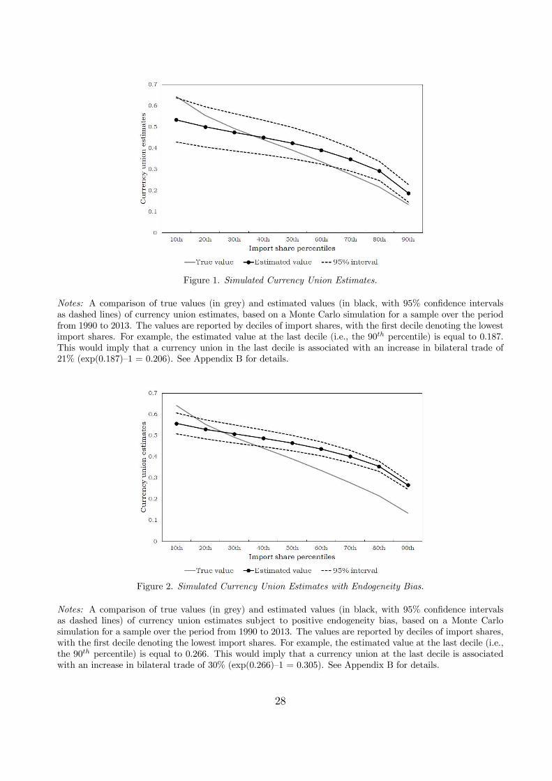
Figure 1. Simulated Currency Union Estimates.

Notes: A comparison of true values (in grey) and estimated values (in black, with 95% con…dence intervalsas dashed lines) of currency union estimates, based on a Monte Carlo simulation for a sample over the periodfrom 1990 to 2013. The values are reported by deciles of import shares, with the …rst decile denoting the lowestimport shares. For example, the estimated value at the last decile (i.e., the 90th percentile) is equal to 0.187.This would imply that a currency union in the last decile is associated with an increase in bilateral trade of21% (exp(0.187)–1 = 0.206). See Appendix B for details.

Figure 2. Simulated Currency Union Estimates with Endogeneity Bias.

Notes: A comparison of true values (in grey) and estimated values (in black, with 95% con…dence intervalsas dashed lines) of currency union estimates subject to positive endogeneity bias, based on a Monte Carlosimulation for a sample over the period from 1990 to 2013. The values are reported by deciles of import shares,with the …rst decile denoting the lowest import shares. For example, the estimated value at the last decile (i.e.,the 90th percentile) is equal to 0.266. This would imply that a currency union at the last decile is associatedwith an increase in bilateral trade of 30% (exp(0.266)–1 = 0.305). See Appendix B for details.

28

It follows that the ξ1 main coe¢cient and the ξ2 interaction coe¢cient in regression (8) are

biased. For the ξ1 main coe¢cient we obtain a highly signi…cant point estimate of ¡0.309,

and for the ξ2 interaction coe¢cient we obtain a highly signi…cant coe¢cient of ¡0.185. Both

coe¢cients are pushed upwards.41 The resulting currency union estimates at the mean, the

10th, and the 90th percentiles follow as 0.431, 0.557, and 0.266 (all signi…cant at the 1% level).

Figures 1 and 2 illustrate the e¤ect of the positive endogeneity bias (we again refer to

Appendix B for details). Both …gures show the true currency union estimates in grey (those

are the same across the two …gures). The black lines show the estimated values (with 95%

con…dence intervals as dashed lines). Figure 1 plots the unbiased currency union estimates in

the absence of endogeneity. Figure 2 plots the corresponding biased estimates when endogeneity

is present. The estimates have roughly the same pro…le in both …gures, indicating relatively

strong currency union e¤ects at low import share percentiles and relatively weak e¤ects at high

percentiles. This is consistent with the empirical results in Section 3. Our estimation procedure

thus correctly identi…es the downward sloping pro…le of currency union e¤ects, validating our

approach. However, the estimates in Figure 2 are pushed upwards especially for high import

shares, ‡attening the pro…le. This means that the gap between the actual and the true estimates

grows for high import shares. Endogeneity thus leads to an overestimation of currency union

e¤ects for country pairs that trade intensively.

Overall, we of course do not observe the precise extent of currency union endogeneity in the

actual data. But our simulation implies that if we were to correct for it, this would strengthen,

rather than weaken, the heterogeneity patterns in our results. Currency union endogeneity

would therefore work against us in the sense that it would make it harder to …nd evidence of

heterogeneity patterns as in Section 3.

Finally, we also run a placebo simulation with endogenous currency unions, assuming that

standard log-linear gravity is the data generating process (as opposed to translog gravity) so

that by construction there is no currency union heterogeneity. We obtain currency union esti-

mates at the mean, the 10th, and the 90th percentiles of 0.298, 0.324, and 0.273 (all signi…cant at

the 1% level).42 These estimates are biased upwards, but they do not exhibit any quantitatively

meaningful pattern of currency union heterogeneity.

6 Robustness

To ensure the robustness of our …ndings, in Appendix C we report a battery of sensitivity checks

based on alternative speci…cations and data samples. As in Section 3, we focus on currency

41The simulated results with endogeneity are directly comparable to those without endogeneity in Table B1where we verify our two-step procedure. In particular, the ξ1 main coe¢cient of ¡0.309 can be compared tothe ¡0.498 coe¢cient in column (3) of Table B1. The ξ2 interaction coe¢cient of ¡0.185 can be compared tothe ¡0.221 coe¢cient in column (3) of Table B1.

42This is in analogy to Appendix B.3. The currency union estimates are directly comparable to those withoutendogeneity in column (3) of Table B2.

29

unions as the main illustration. While the magnitude of the trade e¤ect of currency unions

may vary across speci…cations, we continue to …nd that it falls with bilateral import shares.

In Table C1 we apply the nearest matching estimator of Persson (2001). Our results are

robust to non-random selection on observables. In Table C2 we show that currency unions con-

tinue to be associated with a heterogeneous trade e¤ect once we control for wars, decolonisation

episodes, and missing data (Campbell, 2013; Campbell and Chentsov, 2020). In Table C3 we

distinguish multilateral currency unions (i.e., between countries of similar size and wealth) from

bilateral currency unions (i.e., when a small or poor country adopts the currency of a larger

and richer country, De Sousa, 2012). Our results hold for both types of currency unions.

In Table C4 we classify our currency union observations into three groups: entry (i.e.,

currency unions created during our sample period), exit (i.e., unions that were dissolved), and

continuous (i.e., they existed over the whole sample period). The currency union interaction

terms with log predicted shares are negative for the continuous and exit unions only. But

among the entry currency unions, the common currency interaction term is negative for the

euro.

Table C5 addresses the measurement of import shares per good. First, we use alternative

proxies for the extensive margin ni. We use the Hummels and Klenow (2005) measure, and

we assume that the extensive margin is unity for all exporters. Second, instead of using the

importing country’s GDP to compute the import shares per good, we experiment with total

or manufacturing gross output from the OECD STAN database (in which case our sample is

reduced to 19 OECD importing countries).

In Table C6 we consider three alternative speci…cations for the …rst-step regression (7).

First, in addition to bilateral distance and contiguity we include indicator variables for sharing

a common language, a common coloniser post-1945, pairs in a colonial relationship post-1945,

and for territories that were, or are, part of the same country. Second, we replace bilateral

distance and contiguity with (directional) country pair …xed e¤ects. Third, we let the distance

and contiguity elasticities vary over time (by interacting the two variables with year dummy

variables). For the second-step regression (8), we show that our results remain robust to

including time-varying distance and contiguity variables, a lagged dependent variable, and a

trend for EU countries or for all countries in a currency union in our sample.

In Table C7 we use alternative data samples. We use the 1949–2006 exports and GDP data

from Head et al. (2010), and exports from the International Monetary Fund’s Direction of Trade

Statistics combined with GDP data from the World Bank’s World Development Indicators

between 1960 and 2013. We use a balanced sample between 1994 and 2013. We drop the

countries (mostly island nations) omitted from the analysis of Glick and Rose (2016), the

smaller nations with GDP below 500 million US dollars in 2013, the poorer countries with

GDP per capita below 500 US dollars in 2013, and the post-Soviet states.

30

Finally, in Table C8 we test for ‘feedback e¤ects’ of currency unions as discussed in Baier

and Bergstrand (2007). As in their paper, we restrict our sample to …ve-year intervals from 1953

to 2013. Based on equation (8) we add one lead (i.e., values …ve years ahead) of the currency

union dummy variable and its interaction with log predicted shares, and their coe¢cients are

insigni…cant. Similar to Baier and Bergstrand (2007) we therefore do not …nd evidence of

feedback e¤ects.

7 Concluding Remarks

This paper o¤ers a new approach to estimating a ‡exible gravity equation. Our framework

has variable trade cost elasticities at its core, implying that trade costs do not always have the

same trade e¤ect across all country pairs. To introduce this form of heterogeneity we develop a

gravity framework motivated by a translog gravity equation. This approach generates variable

trade cost elasticities across and within country pairs. The key prediction is that the impact

of trade costs should be larger for country pairs associated with smaller import shares.

We test this prediction by employing an extensive data set of aggregate bilateral import

shares for 199 countries between 1949 and 2013. We apply it to the e¤ect of currency unions

on international trade as well as a host of other trade cost variables that are popular in the

literature such as the formation of regional trade agreements and membership of the WTO.

Our results lend strong support to our theoretical prediction.

For example, we present evidence that the euro has promoted bilateral trade among Euro-

zone members but this e¤ect is heterogeneous across country pairs. Pairs which do not trade

intensively with each other tend to increase their bilateral trade by more in response to joining

the euro currency union. Pairs that already have a strong trading relationship do not increase

bilateral trade at all.

Regarding the trade e¤ect of currency unions in particular, our results shed light on some of

the disparities between estimates reported in the literature. By emphasising that country pairs

with higher import intensity have smaller trade cost elasticities, our framework helps to explain

why PPML currency union estimates are typically smaller than their OLS counterparts. In

addition, as the average import share is signi…cantly larger among euro member pairs compared

to non-euro currency union pairs, our framework also helps to explain why the euro trade e¤ect

typically proves weaker on average. Our results suggest that relying on a single currency union

estimate can be misleading if the objective is to assess, or to predict, the impact of a common

currency on bilateral trade.

Although in our empirical application we study the trade e¤ect of currency unions in most

detail, we also demonstrate that the predictions of our theoretical framework apply more gen-

erally to a broader set of trade cost-related variables including RTAs, WTO membership,

distance, sharing a common border, a common language, and tari¤s. These results provide

31

strong evidence that the aggregate trade cost elasticity is variable and heterogeneous across

country pairs. One potential implication is that the gains from trade liberalisation could be

mismeasured if researchers erroneously assume a constant trade cost elasticity (Arkolakis et

al., 2012; Melitz and Redding, 2015; Bas et al., 2017). Although exploring this aspect remains

outside the scope of this paper, understanding the welfare implications of our results would be

an important next step.

University of Warwick, CAGE, CESifo, and CEPR

University of Warwick, CAGE, CEP/LSE, CESifo, and CEPR

32

References

Alesina, A. and Barro, R.J. (2002). ‘Currency unions’, Quarterly Journal of Economics, vol.

117(2), pp. 409–36.

Alesina, A., Barro, R.J. and Tenreyro, S. (2002). ‘Optimal currency areas’, NBER Macroeco-

nomics Annual, vol. 17, pp. 301–45.

Anderson, J. and van Wincoop, E. (2003). ‘Gravity with gravitas: a solution to the border

puzzle’, American Economic Review, vol. 93(1), pp. 170–92.

Arkolakis, C., Costinot, A. and Rodríguez-Clare, A. (2012). ‘New trade models, same old

gains?’, American Economic Review, vol. 102(1), pp. 94–130.

Atkeson, A. and Burstein, A. (2008). ‘Trade costs, pricing-to-market, and international relative

prices’, American Economic Review, vol. 98(5), pp. 1998–2031.

Baier, S.L. and Bergstrand, J.H. (2007). ‘Do free trade agreements actually increase members’

international trade?’, Journal of International Economics, vol. 71(1), pp. 72–95.

Baier, S.L., Yotov, Y.V. and Zylkin, T. (2019). ‘On the widely di¤ering e¤ects of free trade

agreements: lessons from twenty years of trade integration’, Journal of International Eco-

nomics, vol. 116, pp. 206–26.

Baldwin, R. (2006). ‘In or out: does it matter? An evidence-based analysis of the euro’s trade

e¤ect’, Centre for Economic Policy Research, London.

Baldwin, R., Di Nino, V., Fontagné, L., De Santis, R.A. and Taglioni, D. (2008). ‘Study on

the impact of the euro on trade and foreign direct investment’, European Economy Economic

Paper 321, European Commission.

Baldwin, R. and Taglioni, D. (2007). ‘Trade e¤ects of the euro: a comparison of estimators’,

Journal of Economic Integration, vol. 22(4), pp. 780–818.

Barro, R. and Tenreyro, S. (2007). ‘Economic e¤ects of currency unions’, Economic Inquiry,

vol. 45(1), pp. 1–23.

Bas, M., Mayer, M. and Thoenig, M. (2017). ‘From micro to macro: demand, supply, and

heterogeneity in the trade elasticity’, Journal of International Economics, vol. 108, pp. 1–19.

Berger, H. and Nitsch, V. (2008). ‘Zooming out: the trade e¤ect of the euro in historical

perspective’, Journal of International Money and Finance, vol. 27(8), pp. 1244–60.

Bergin, P.R. and Lin, C.-Y. (2012). ‘The dynamic e¤ects of a currency union on trade’, Journal

of International Economics, vol. 87(2), pp. 191–204.

33

Berthou, A. and Fontagné, L. (2008). ‘The euro e¤ects on the …rm and product-level trade

margins: evidence from France’, CEPII Working Paper 2008–21.

Broda, C. and Romalis, J. (2010). ‘Identifying the relationship between trade and exchange

rate volatility’, in (I. Takatoshi and A.K. Rose, eds.), Commodity Prices and Markets, East

Asia Seminar on Economics, Volume 20, University of Chicago Press, Chicago, pp. 79–110.

Bun, M.J.G. and Klaassen, F.J.M. (2007). ‘The euro e¤ect on trade is not as large as commonly

thought’, Oxford Bulletin of Economics and Statistics, vol. 69(4), pp. 473–96.

Campbell, D.L. (2013). ‘Estimating the impact of currency unions on trade: solving the Glick

and Rose puzzle’, The World Economy, vol. 36(10), pp. 1278–93.

Campbell, D.L. and Chentsov, A. (2020). ‘Breaking badly: the currency union e¤ect on trade’,

New Economic School Working Paper 265.

Carrère, C., Mrázová, M. and Neary, J.P. (2020). ‘Gravity without apology: the science of

elasticities, distance, and trade’, Economic Journal, vol. 130(628), pp. 880–910.

Chaney, T. (2008). ‘Distorted gravity: the intensive and extensive margins of international

trade’, American Economic Review, vol. 98(4), pp. 1707–21.

Chen, N. and Novy, D. (2018). ‘Currency unions, trade, and heterogeneity’, CEPR Discussion

Paper 12954.

Correia, S., Guimarães, P. and Zylkin, T. (2020). ‘Fast poisson estimation with high-

dimensional …xed e¤ects’, Stata Journal, vol. 20(1), pp. 95–115.

De Nardis, S. and Vicarelli, C. (2003). ‘Currency unions and trade: the special case of EMU’,

Review of World Economics, vol. 139(4), pp. 625–49.

De Sousa, J. (2012). ‘The currency union e¤ect on trade is decreasing over time’, Economics

Letters, vol. 117(3), pp. 917–20.

Devereux, M.B. and Lane, P.R. (2003). ‘Understanding bilateral exchange rate volatility’, Jour-

nal of International Economics, vol. 60(1), pp. 109–32.

Eaton, J. and Kortum, S. (2002). ‘Technology, geography, and trade’, Econometrica, vol. 70(5),

pp. 1741–79.

Eaton, J., Kortum, S. and Sotelo, S. (2013). ‘International trade: linking micro to macro’, in (D.

Acemoglu, M. Arellano and E. Dekel, eds.), Advances in Economics and Econometrics Tenth

World Congress, Volume 2: Applied Economics, Cambridge University Press, Cambridge, pp.

329–70.

Eicher, T.S. and Henn, C. (2011). ‘One money, one market: a revised benchmark’, Review of

International Economics, vol. 19(3), pp. 419–35.

34

Feenstra, R.C. (2003). ‘A homothetic utility function for monopolistic competition models,

without constant price elasticity’, Economics Letters, vol. 78(1), pp. 79–86.

Felbermayr, G., Larch, M., Yalcin, E. and Yotov, Y.V. (2020). ‘On the heterogeneous trade

and welfare e¤ects of GATT/WTO membership’, CESifo Working Paper 8555.

Flam, H. and Nordström, H. (2007). ‘Explaining large euro e¤ects on trade: the extensive

margin and vertical specialization’, Institute for International Economic Studies, Stockholm

University, mimeo.

Frankel, J. (2010). ‘The estimated trade e¤ects of the euro: why are they below those from

historical monetary unions among smaller countries?’, in (A. Alesina and F. Giavazzi, eds.),

Europe and the Euro, University of Chicago Press, Chicago, pp. 169–212.

Frankel, J. and Rose, A. (2002). ‘An estimate of the e¤ect of common currencies on trade and

income’, Quarterly Journal of Economics, vol. 117(2), pp. 437–66.

Glick, R. (2017). ‘Currency unions and regional trade agreements: EMU and EU e¤ects on

trade’, Comparative Economic Studies, vol. 59(2), pp. 194–209.

Glick, R. and Rose, A.K. (2002). ‘Does a currency union a¤ect trade? The time-series evidence’,

European Economic Review, vol. 46(6), pp. 1125–51.

Glick, R. and Rose, A.K. (2016). ‘Currency unions and trade: a post-EMU reassessment’,

European Economic Review, vol. 87, pp. 78–91.

Head, K. and Mayer, T. (2014). ‘Gravity equations: workhorse, toolkit, and cookbook’, in (G.

Gopinath, E. Helpman and K. Rogo¤, eds.), Handbook of International Economics, Chapter 3,

pp. 131–95.

Head, K., Mayer, T. and Ries, J. (2010). ‘The erosion of colonial linkages after independence’,

Journal of International Economics, vol. 81(1), pp. 1–14.

Helpman, E., Melitz, M. and Rubinstein, Y. (2008). ‘Estimating trade ‡ows: trading partners

and trading volumes’, Quarterly Journal of Economics, vol. 123(2), pp. 441–87.

Hummels, D. and Klenow, P.J. (2005). ‘The variety and quality of a nation’s exports’, American

Economic Review, vol. 95(3), pp. 704–23.

Irarrazabal, A., Moxnes, A. and Opromolla, L.D. (2015). ‘The tip of the iceberg: a quantitative

framework for estimating trade costs’, Review of Economics and Statistics, vol. 97(4), pp. 777–

92.

Klein, M.W. (2005). ‘Dollarization and trade’, Journal of International Money and Finance,

vol. 24(6), pp. 935–43.

35

Klein, M.W. and Shambaugh, J.C. (2006). ‘Fixed exchange rates and trade’, Journal of Inter-

national Economics, vol. 70(2), pp. 359–83.

Larch, M., Wanner, J., Yotov, Y. and Zylkin, T. (2019). ‘Currency unions and trade: a PPML

re-assessment with high-dimensional …xed e¤ects’, Oxford Bulletin of Economics and Statistics,

vol. 81(3), pp. 487–510.

López-Córdova, J.E. and Meissner, C.M. (2003). ‘Exchange-rate regimes and international

trade: evidence from the classical gold standard era’, American Economic Review, vol. 93(1),

pp. 344–53.

Mayer, T., Vicard, V. and Zignago, S. (2019). ‘The cost of non-Europe, revisited’, Economic

Policy, vol. 34(98), pp. 147–99.

Melitz, M.J. and Ottaviano, G.I.P. (2008). ‘Market size, trade, and productivity’, Review of

Economic Studies, vol. 75(1), pp. 295–316.

Melitz, M.J. and Redding, S.J. (2015). ‘New trade models, new welfare implications’, American

Economic Review, vol. 105(3), pp. 1105–46.

Micco, A., Stein, E. and Ordoñez, G. (2003). ‘The currency union e¤ect on trade: early evidence

from EMU’, Economic Policy, vol. 37(18), pp. 315–56.

Mika, A. and Zymek, R. (2018). ‘Friends without bene…ts? New EMU members and the “euro

e¤ect” on trade’, Journal of International Money and Finance, vol. 83, pp. 75–92.

Mundell, R.A. (1961). ‘A theory of optimum currency areas’, American Economic Review, vol.

51(4), pp. 657–65.

Nitsch, V. (2002). ‘Honey, I shrunk the currency union e¤ect on trade’, The World Economy,

vol. 25(4), pp. 457–74.

Novy, D. (2013). ‘International trade without CES: estimating translog gravity’, Journal of

International Economics, vol. 89(2), pp. 271–82.

Parente, P.M.D.C. and Santos Silva, J.M.C. (2016). ‘Quantile regression with clustered data’,

Journal of Econometric Methods, vol. 5(1), pp. 1–5.

Persson, T. (2001). ‘Currency unions and trade: how large is the treatment e¤ect?’, Economic

Policy, vol. 33(16), pp. 434–48.

Rose, A.K. (2000). ‘One money, one market: estimating the e¤ect of common currencies on

trade’, Economic Policy, vol. 30(15), pp. 8–45.

Rose, A.K. (2001). ‘Currency unions and trade: the e¤ect is large’, Economic Policy, vol.

16(33), pp. 449–61.

36

Rose, A.K. (2005). ‘Which international institutions promote international trade?’, Review of

International Economics, vol. 13(4), pp. 682–98.

Rose, A.K. (2006). ‘Currency unions’, in (S.N. Durlauf and L.E. Blume, eds.), The New Palgrave

Dictionary of Economics, Second Edition, Palgrave Macmillan, 2008.

Rose, A. and van Wincoop, E. (2001). ‘National money as a barrier to international trade: the

real case for currency union’, American Economic Review, vol. 91(2), pp. 386–90.

Saia, A. (2017). ‘Choosing the open sea: the cost to the UK of staying out of the euro’, Journal

of International Economics, vol. 108, pp. 82–98.

Santos Silva, J.M.C. and Tenreyro, S. (2006). ‘The log of gravity’, Review of Economics and

Statistics, vol. 88(4), pp. 641–58.

Santos Silva, J.M.C. and Tenreyro, S. (2010). ‘Currency unions in prospect and retrospect’,

Annual Review of Economics, vol. 2, pp. 51–74.

Spearot, A.C. (2013). ‘Variable demand elasticities and tari¤ liberalization’, Journal of Inter-

national Economics, vol. 89(1), pp. 26–41.

Subramanian, A. and Wei, S.-J. (2007). ‘The WTO promotes trade, strongly but unevenly’,

Journal of International Economics, vol. 72(1), pp. 151–75.

37

A Data

Bilateral Exports The International Monetary Fund’s Direction of Trade Statistics (DOTS)

is the most widely used data set for studying the e¤ect of currency unions on international trade.

For more than 200 countries between 1948 and 2014, it reports bilateral FOB merchandise

exports (in US dollars) of which 46% are recorded as zero. Head et al. (2010) argue that the

true value of many of the zero export ‡ows reported by the DOTS is likely to be positive.

Relying on alternative data sources, they identify a number of problematic zeros and replace

them by positive values or set them as missing entries. They also …x a number of typos due

to incorrect reporting between FOB and CIF values. We rely on the data set cleaned by Head

et al. (2010) for our analysis. As their data set only spans the period from 1948 to 2006, we

update their series up to 2014 using the growth rates of positive exports reported by the DOTS.

GDPs and Populations Nominal GDPs (in US dollars) and populations between 1949 and

2006 are from the Centre d’Etudes Prospectives et d’Informations Internationales (CEPII).

We update them up to 2013 using the growth rates of GDPs and populations from the World

Bank’s World Development Indicators (WDI).

Gravity Gravity controls are from CEPII. These include bilateral (population weighted)

distances (in kilometres), and dummies for sharing a common land border (contiguity), a

common (o¢cial) language, a common coloniser post-1945, pairs in a colonial relationship

post-1945, and for pairs that were, or are, the same country. Dummy variables for membership

with the OECD, IMF, and WTO are constructed using online sources (the dummies are equal

to one if both countries in a pair are members in each year, and zero otherwise).

We create a dummy variable for country pairs in an RTA using two di¤erent sources: CEPII

between 1948 and 2006 and De Sousa (2012) between 1958 and 2014. As it contains a larger

number of observations for pairs in an RTA between 1958 and 2006 (for instance, it reports the

RTA between Thailand and Laos since 1991), we rely on the CEPII series and carry forward

the RTA observations up to 2014. Based on De Sousa (2012), we then update the CEPII series

in three ways: 1) we add the RTAs created after 2006 (for instance, between the EU and Peru

and Colombia since 2013), 2) we identify countries that left an RTA after 2006 (for instance,

Angola left the COMESA in 2007), and 3) we add a few missing RTAs prior to 2007 (for

instance, the RTA between the EU and the Faroe Islands since 1997).

Currency Unions De Sousa (2012) provides information on currency union membership be-

tween 1948 and 2014. He identi…es three types of currency unions: 1) bilateral currency unions,

which ‘commonly occur when a small and/or poor country unilaterally adopts the money of a

larger, richer ‘anchor’ country’ (Rose, 2006), 2) multilateral currency unions ‘between countries

of more or less equal size and wealth’ (Rose, 2006), and 3) cases where ‘money was interchange-

able between the two countries at a 1:1 par for an extended period of time, so that there was

38

no need to convert prices when trading between a pair of countries.’

The data set of De Sousa (2012) covers 230 countries between 1948 and 2014 and includes

58,534 currency union observations. Between 1949 and 2013, which is the time period we focus

on in our paper, this number drops to 54,648. In our sample, we only observe 19,514 currency

union observations (see Table A1 below).43 There are several reasons for this discrepancy.

First, a number of currency union countries are omitted from the Head et al. (2010) data set.

These include American Samoa, Belgium, Guam, Monaco, Luxembourg, and Montenegro (De

Sousa, 2012, reports data for Belgium and Luxembourg both separately and as a single entity

while we merge them over the entire period). Second, for other currency union countries the

import shares per good cannot be calculated if either bilateral exports, the importer’s GDP,

or the extensive margin are missing: Montserrat, San Marino, and Wallis and Futuna have

no trade data; the Falkland Islands, Gibraltar, Nauru, and Saint Helena have no extensive

margin and GDP data; Guadeloupe, French Guiana, Martinique, Réunion, and Saint Pierre

et Miquelon are omitted as importers as they have no GDP data; Andorra is excluded as an

importer because in the sample it only imports from Taiwan which is missing extensive margin

data; Equatorial Guinea is omitted as an exporter because it lacks extensive margin data.

Other countries which never belonged to a currency union are also excluded from our data

set: Anguilla, British Virgin Islands, Cocos Islands, Cook Islands, Christmas Island, Cayman

Islands, Micronesia, Marshall Islands, Northern Mariana Islands, Norfolk Island, Niue, the

Palestinian Territory, Pitcairn, Puerto Rico, Turks and Caicos Islands, Tokelau, and Western

Sahara have no trade data; North Korea, Taiwan, and Uzbekistan are excluded as exporters

because of missing extensive margin data; Timor-Leste is excluded as an importer because in

the sample it only imports from Taiwan which has no extensive margin data.

Descriptive Statistics As the pre-1997 trade ‡ows for Belgium and Luxembourg are re-

ported jointly, we merge the two countries into a single entity over the entire period (and we

count the two countries as one). Our sample therefore includes 199 countries between 1949

and 2013. Bilateral import shares are given by the ratio between bilateral exports and the

importing country’s GDP, and we discard outliers by excluding the highest import shares that

represent 0.05% of the sample size. Bilateral import shares per good are then obtained by di-

viding the import shares by the average over time of the number of product categories exported

by each country as a share of the total number of categories exported by all countries in each

year (from United Nations Comtrade). See Section 3.1.1 for more details.

As shown in Table A1, our full sample includes 1,203,583 observations of which 782,469

import shares (and import shares per good) are positive, and 421,114 are equal to zero (i.e.,

43Togo has been using the CFA franc since 1945. In De Sousa’s (2012) data set, the currency union dummyfor Togo with the other countries using the CFA franc is equal to one in all years except 1962. As this dummyis equal to one in 1962 in the data set of Glick and Rose (2016), we switched its value from zero to one in 1962.

39

Table A1. Descriptive Statistics.Full sample Positive import shares

Number of observations 1,203,583 782,469

Number of zero import shares 421,114 0

Number of positive import shares 782,469 782,469

Import shares

Minimum 0.000% 0.001%

Maximum 41.264% 41.264%

Mean 0.290% 0.447%

Standard deviation 1.522% 1.869%

Number of observations for currency unions 19,514 13,085

Number of pairs in a currency union (directional) 1,255 924

Number of switches into currency unions (directional) 379 342

Number of switches out of currency unions (directional) 782 459

Source: Authors’ calculations.

35% of the sample).44 The lowest positive import share is close to zero (from Angola to

Colombia), and the largest is equal to 41.3% (from Singapore to the Maldives). The mean and

standard deviation of import shares are equal to 0.3% and 1.5% (0.4% and 1.9% in the sample

of positive shares). As the import shares per good are given by the import shares over the

extensive margin, they do not have any meaningful units and are therefore not described in the

table. In the full sample, 1,255 country pairs (directional) share a common currency at some

point (amounting to 19,514 observations, or about 1.6% of the sample). There are 379 and 782

country pairs (directional) that switched into or out of currency unions.

Table A2. Currency Unions and Non-Unions.Currency Unions Non-Unions

Import share (%) 1.061 (3.897) 0.278 (1.447)

RTA 0.292 (0.454) 0.048 (0.214)

WTO 0.564 (0.496) 0.419 (0.493)

OECD 0.099 (0.298) 0.025 (0.157)

IMF 0.690 (0.462) 0.731 (0.443)

ln Distance 7.645 (0.972) 8.720 (0.768)

Contiguity 0.144 (0.351) 0.019 (0.138)

Shared language 0.712 (0.453) 0.164 (0.370)

Common coloniser 0.597 (0.490) 0.094 (0.292)

Colonial relationship 0.057 (0.232) 0.009 (0.097)

Same country 0.174 (0.379) 0.007 (0.086)

Observations 19,514 1,184,069

Notes: The table reports the mean and standard deviation (in parentheses) of each variable.

44Note that in the empirical analysis, for instance in column (3) of Table 1, the sample size may be reducedas singleton observations are dropped due to the inclusion of …xed e¤ects.

40

Table A2 provides descriptive statistics for currency unions and non-unions in the full

sample (including the zero import shares). For most variables, the sample means are similar

for the two groups of countries (standard deviations are reported between parentheses). Still,

countries in a currency union have higher import shares, are closer, are more likely to be in a

colonial relationship and to belong to the OECD and WTO, and are less likely to belong to

the IMF.

B Theory and Monte Carlo Analysis

In Section B.1 we outline the derivation of the translog gravity equation. In Section B.2 we

carry out a Monte Carlo simulation under the assumption that the translog gravity model with

variable trade cost elasticities is the data generating process. The aim is to con…rm that our

two-step procedure in Section 3 is able to detect the heterogeneity of trade cost e¤ects implied

by variable trade cost elasticities. In Section B.3 we carry out a Monte Carlo simulation under

the assumption that the standard log-linear gravity model with a constant trade cost elasticity

is the data generating process. This is a placebo check in the sense that under this assumption,

we should not …nd heterogeneous trade cost e¤ects with our two-step procedure. In Section B.4

we compute general equilibrium e¤ects to rule out that those might explain the heterogeneity

patterns we …nd in the data.

B.1 Derivation of the Translog Gravity Equation

We derive the translog gravity equation (1). We refer to Novy (2013) for further details. The

translog expenditure function for country j is given by:

ln(Ej) = ln(Uj) + α0j +NX

m=1

αm ln(pmj) +1

2

NX

m=1

NX

k=1

θkm ln(pmj) ln(pkj),

where Ej is expenditure, Uj is the utility level, with m and k indexing goods and θkm = θmk.

The price of good m when delivered in country j is denoted by pmj, where pmj = tmjpm and

pm denotes the price of good m net of trade costs. We assume symmetry across goods from

the same origin country i in the sense that pm = pi for all goods m originating in country i,

and the corresponding bilateral trade costs to country j are also symmetric, i.e., tmj = tij.

As in Feenstra (2003) we impose the following parameter restrictions to ensure homogeneity

of degree one:NX

m=1

αm = 1 andNX

k=1

θkm = 0.

We further impose that goods enter symmetrically:

θmm = ¡θ

N(N ¡ 1) and θkm =

θ

Nfor k 6= m,

41

with θ > 0.

The expenditure share smj of country j on good m can be obtained by di¤erentiating the

expenditure function with respect to ln(pmj):

smj = αm +NX

k=1

θkm ln(pkj).

The import share corresponding to bilateral trade xij from country i to country j follows as:

xijyj=

X

mi

smj ,

where the individual import shares smj are summed up over all goods m originating in country

i. To close the model we impose market clearing:

yi =SX

j=1

xij,

where S denotes the number of countries in the world.

To obtain the translog gravity equation we substitute the import shares into the market

clearing condition. Using pkj = tkjpk we solve for the net prices pk and substitute them back

into the expenditure shares and import shares. This yields the translog gravity equation (1).

B.2 Analysis of the Two-Step Procedure

When running PPML gravity regressions in Section 3, we adopt a two-step procedure to esti-

mate heterogeneous currency union e¤ects. In the …rst step, we predict the import shares per

good. In the second step, we interact the currency union dummy with the log predicted shares.

In this section we carry out Monte Carlo simulations to verify the validity of this two-step

procedure.

As our trade cost function, we assume:

ln(tij,t) = κCUij,t + ζWij,t, (B.1)

where Wij,t contains bilateral trade cost variables used in our analysis other than currency

unions, i.e., time-invariant geography-related variables (logarithmic bilateral distance and a

contiguity dummy) as well as time-varying policy variables (dummies for RTAs and membership

of the WTO, OECD, and IMF). We choose values for the trade cost parameters that are derived

from our baseline regression in column (3) of Table 1.45 We then compute trade costs on the

basis of equation (B.1) using the actual observations for our trade cost variables.

45Assuming an elasticity of substitution of σ = 5 for the constant elasticity gravity framework implied by

42

We assume that the data generating process is given by the translog gravity model in

Section 2. We choose the translog parameter value as θ = 0.095.46 Based on equations (1) to

(3), we …rst compute the import shares in a deterministic way (i.e., without an error term).

We use a balanced sample of observed data for the GDP variables (yi,t, yj,t), the extensive

margin measure ni, and the trade cost variables underlying equation (B.1) for 120 origin and

destination countries over the period from 1990 to 2013.47

Then we include an additive error term in the translog gravity equation (1). We choose

its standard deviation to match the share of zero observations in the sample (Santos Silva and

Tenreyro, 2006).48 We then run …rst-step and second-step regressions as in column (5) of Table

1. In the …rst step we predict import shares per good, and in the second step we interact the

currency union dummy with the log predicted shares. Standard errors are clustered at the

non-directional country pair level. We run 100 iterations of this procedure, drawing a new set

of errors for every iteration.

We report the results in Table B1. For reference, column (1) shows the true currency union

estimates, evaluated at the mean, the 10th, and the 90th percentiles of log predicted import

shares (as in Section 3, calculated for non-zero import shares only). The reported coe¢cients

and standard errors in columns (2) and (3) are averaged over all iterations. Analogous to

speci…cation (7), the …rst-step regression in column (2) simply includes distance and a contiguity

dummy in addition to time-varying exporter and importer …xed e¤ects. Distance and contiguity

have the expected signs. The second-step regression in column (3) includes the currency union

dummy and an interaction term with the log predicted import share, as well as the additional

time-varying policy variables and …xed e¤ects. Consistent with column (5) of Table 1, we obtain

negative and highly signi…cant coe¢cients on the currency union dummy and the interaction

term. The lower panel of column (3) reports the implied currency union estimates, evaluated

at the mean, the 10th, and the 90th percentiles of log predicted import shares. We …nd a

mean estimate of 0.384, implying that evaluated at the average import share, two countries

trade 46.8% more bilaterally if they are in a currency union. Consistent with the theoretical

framework, we …nd a larger estimate of 0.533 at the 10th percentile (i.e., for relatively small

import shares), implying 70.4% more bilateral trade ceteris paribus. At the 90th percentile (i.e.,

for relatively large import shares) we …nd an estimate of 0.187, implying increased bilateral

column (3) of Table 1, the κ parameter for the currency union dummy in equation (B.1) follows as the estimatedcoe¢cient of 0.252 in column (3) of Table 1 divided by (1¡σ), i.e., κ = 0.252/(1¡5) = ¡0.063. The parametersfor the RTA, WTO, OECD, and IMF variables follow analogously as ¡0.032, 0.001, ¡0.148, and ¡0.051. Toobtain parameter values for distance and contiguity in (B.1), we run a regression as in equation (7) based onthe observed import shares per good, with estimated coe¢cients of ¡0.747 and 0.881 (both signi…cant at the1% level). The parameters thus follow as 0.187 and ¡0.220.

46In the translog regression in column (1) of Table 6, we obtain a currency union coe¢cient of 0.006. Assumingthe same currency union coe¢cient as above, it therefore follows θ = ¡0.006/κ = 0.095.

47To reduce computing time we use a subset of data starting in 1990.48Similar to Santos Silva and Tenreyro (2006), we round values to zero (the nearest integer), in this case for

su¢ciently negative errors that would otherwise imply negative trade shares. The share of zero observations isaround 17% in the simulation sample.

43

Table B1. Monte Carlo Simulation.(1) (2) (3)

First step Second step

CU – ¡0.498(0.118)

¤¤¤

CU£ ln predicted share – ¡0.221(0.035)

¤¤¤

RTA – 0.074(0.007)

¤¤¤

WTO – 0.021(0.017)

OECD – 0.492(0.030)

¤¤¤

IMF – 0.117(0.066)

¤

ln Distance ¡0.537(0.011)

¤¤¤ –

Contiguity 0.276(0.031)

¤¤¤ –

CU estimates True Estimated

Mean 0.326 – 0.384(0.032)

¤¤¤

10th percentile 0.643 – 0.533(0.053)

¤¤¤

90th percentile 0.134 – 0.187(0.021)

¤¤¤

Observations 223,095 222,937

Corresponding table (column) – Table 1 (column 5)

Notes: Exporter-year and importer-year …xed e¤ects are included. Directional country pair …xed e¤ects arefurther included in (3). The regressions are estimated with PPML for data from 1990 to 2013 with the importshare per good as the dependent variable. Translog gravity is the data generating process (with the truecurrency union estimates reported in the …rst column). The reported coe¢cients are averages over 100 iterations.Robust standard errors clustered at the (non-directional) country pair level are reported in parentheses (notbootstrapped), also averaged over 100 iterations. ¤¤¤ and ¤ indicate signi…cance at the 1% and 10% levels,respectively. ‘predicted share’ is the predicted import share.

trade by 20.6%. These estimates can be compared to the true values underlying the simulation

indicated in column (1).

Overall, the simulation in Table B1 con…rms the validity of our two-step procedure in the

sense that qualitatively, it yields heterogeneous currency union estimates as in the underlying

model. Quantitatively, the heterogeneity pro…le is not quite as steep as suggested by the

theoretical model, with our results slightly undershooting the true e¤ect at the 10th percentile

and slightly overshooting at the 90th percentile. Figure 1 visually compares the true values

against the estimates across all deciles of (predicted) import shares. 95% con…dence intervals

are indicated as dashed lines. The true values lie within the con…dence intervals, except for

smallest and largest percentiles. The reason for the relatively steeper heterogeneity pro…le of

the true values is the functional form of the translog speci…cation. As equation (4) shows,

the translog elasticity is given by the translog preference parameter divided by the import

share. This can generate a hyperbolic shape with very large elasticities for the smallest import

44

shares.49

As an additional check, we also investigate the consequences of ignoring the …rst step alto-

gether by erroneously interacting the currency union dummy with log actual import shares (as

opposed to log predicted import shares). Since in that case the interacted regressor is by con-

struction positively correlated with the dependent variable, this leads to an upward endogeneity

bias on the interaction coe¢cient. In fact, it even turns positive with high signi…cance. The

resulting estimates at the mean, the 10th, and the 90th percentiles follow as ¡0.540, ¡1.422,

and 0.244 (all signi…cant at the 1% level). Thus, they exhibit the opposite pattern of the

true values in Table B1 in that they rise with the import share.50 This is incorrect and we

strongly advise against such a speci…cation. This check therefore underlines the importance of

predicting shares in the …rst step.

B.3 Placebo Check

We also carry out a placebo check that is based on the assumption that the standard log-linear

gravity model represents the data generating process. We construct the import shares for the

standard gravity model using the relationship:

xij,tyj,t

=yi,tyWt

µtij,t

Pi,tPj,t

¶1¡σ

, (B.2)

which is derived by Anderson and van Wincoop (2003). Pi,t and Pj,t denote the price indices

of the origin and destination countries, or multilateral resistance terms, given by:

P 1¡σi,t =

SX

s=1

P σ¡1s,t

ys,tyWt

t1¡σsi,t , (B.3)

where S is the number of countries in the world. We assume σ = 5. We use equations (B.2) and

(B.3) as well as trade cost function (B.1) to construct the deterministic import shares, based

on the same sample of GDP and trade cost variables for 120 countries as above. We solve

for the price indices numerically through iteration. Similarly as above, we include an additive

error term in the gravity equation, choosing its standard deviation to match the share of zero

observations in the sample. We then run …rst-step and second-step regressions estimated with

PPML, iterating the procedure 100 times with fresh error terms.

We report the results of the placebo check in Table B2. Column (1) shows the true currency

union estimates. By construction they are the same when evaluated at di¤erent percentiles

of simulated import shares. The …rst-step regression in column (2) includes coe¢cients on

distance and contiguity with the expected signs. The second-step regression in column (3)

49Also see the discussion in Section 3.2.50See column (4) in Table 1 where currency union estimates also (erroneously) rise with the import share.

45

Table B2. Monte Carlo Simulation (Placebo Check).(1) (2) (3)

First step Second step

CU – 0.269(0.008)

¤¤¤

CU£ ln predicted share – 0.006(0.003)

¤

RTA – 0.124(0.002)

¤¤¤

WTO – ¡0.006(0.004)

¤

OECD – 0.576(0.007)

¤¤¤

IMF – 0.200(0.011)

¤¤¤

ln Distance ¡0.795(0.005)

¤¤¤ –

Contiguity 0.978(0.015)

¤¤¤ –

CU estimates True Estimated

Mean 0.252 – 0.235(0.010)

¤¤¤

10th percentile 0.252 – 0.222(0.016)

¤¤¤

90th percentile 0.252 – 0.249(0.003)

¤¤¤

Observations 223,095 223,002

Corresponding table (column) – Table 1 (column 5)

Notes: Exporter-year and importer-year …xed e¤ects are included. Directional country pair …xed e¤ects arefurther included in (3). The regressions are estimated with PPML for data from 1990 to 2013 with the importshare as the dependent variable. Standard gravity is the data generating process (with the true currencyunion estimates reported in the …rst column). The reported coe¢cients are averages over 100 iterations.Robust standard errors clustered at the (non-directional) country pair level are reported in parentheses (notbootstrapped), also averaged over 100 iterations. ¤¤¤ and ¤ indicate signi…cance at the 1% and 10% levels,respectively. ‘predicted share’ is the predicted import share.

exhibits a currency union interaction term that is only marginally signi…cant but with the

opposite (positive) sign compared to our …ndings in Section 3. The positive sign would imply

a heterogeneity pro…le that rises with the import share. In any case, the estimated currency

union e¤ects reported in the lower panel are quantitatively very close and not signi…cantly

di¤erent from the true e¤ects in column (1).

Overall, the placebo results con…rm that if standard gravity is the underlying model, our

two-step procedure does not give rise to currency union e¤ects that vary across import shares

in a meaningful way.

B.4 General Equilibrium E¤ects

Our results on the heterogeneity of currency union e¤ects reported in Section 3 refer to the

direct e¤ect of trade costs on trade (also see our discussion of the trade cost elasticity in Section

2). However, a change in trade costs also has an indirect e¤ect on trade through changes in

46

multilateral resistance in general equilibrium, a point famously made by Anderson and van

Wincoop (2003). The aim of this appendix is to trace out these general equilibrium e¤ects

in response to a change in trade costs. We show that they cannot explain the heterogeneity

patterns in Section 3.

First, we base our analysis on the standard gravity model as in equation (B.2). Similar to

Novy (2013) we take logarithms and …rst di¤erences to arrive at:

¢ ln

µxij,tyj,t

¶

= (1¡ σ)¢ ln (tij,t) + (σ ¡ 1)¢ ln (Pi,tPj,t) + ¢ ln

µyi,tyWt

¶

. (B.4)

The left-hand side represents the percentage change in the import share. The …rst term on the

right-hand side represents the direct e¤ect of the change in trade costs. The second and third

terms indicate the indirect general equilibrium e¤ects, consisting of changes in multilateral

resistance and the change in the exporting country’s income share.

With the help of decomposition (B.4) we analyse a counterfactual change in trade costs.

As in Appendix B.2 we draw on a sample of 120 origin and destination countries, using the

observed data for the GDP variables (yi,t, yj,t) and the trade cost variables underlying equation

(B.1) with the same parameter values as in that section. In particular, the value of the currency

union dummy coe¢cient κ is chosen such that it matches the 0.252 coe¢cient in column (3)

of Table 1, and as previously we assume σ = 5. Based on those data we numerically compute

an initial equilibrium under the assumption of no currency unions (i.e., we set CUij,t to zero

for all pairs). As our counterfactual exercise, we then compute a new equilibrium under the

assumption that a currency union is formed for a particular pair (i.e., we set CUij,t to one

such that tij,t changes for that particular pair). We then compute the terms in decomposition

(B.4), assuming that the exporting country’s income share is constant.51 We compute such a

counterfactual equilibrium for each of the currency union pairs in our sample. We use data for

a single-cross section (for the year 2000), in which the data indicate 244 currency union pairs.

Thus, we compute 244 counterfactual equilibria.

We present the results in Table B3. Since we are interested in variation across import

shares, we report the results as averages across import share intervals for currency union pairs.

Speci…cally, we choose three import share intervals in ascending order based on the initial

equilibrium. For example, the …rst row of Table B3 reports the average changes for currency

union pairs that fall in the tercile of the smallest import shares in the initial equilibrium. By

construction the direct e¤ect in column (2) re‡ects the 0.252 currency union dummy coe¢cient

from column (3) of Table 1. That is, entering into a currency union is associated with an

increase in bilateral trade of 29% (equal to exp (0.252) ¡ 1). The indirect e¤ect operating

through changes in multilateral resistance in column (3) is quantitatively small. The intuition

51That is, ¢ln¡yi,t/y

Wt

¢= 0. The e¤ect operating through a changing income share is typically negligibly

small. Since we hold income shares …xed, our results can be described as ‘modular trade impact’ in theterminology of Head and Mayer (2014).

47

Table B3. General Equilibrium E¤ects (Standard Gravity).Total e¤ect Direct e¤ect Indirect GE e¤ect

¢ln (xij,t/yj,t) = (1 ¡ σ)¢ ln (tij,t) + (σ ¡ 1)¢ ln (Pi,tPj,t)

Import share interval (1) (2) (3)

First interval 0.246 = 0.252 + ¡0.006

Second interval 0.251 = 0.252 + ¡0.001

Third interval 0.242 = 0.252 + ¡0.010

Notes: This table is based on the decomposition in equation (B.4). It reports logarithmic di¤erences between

the initial equilibrium and counterfactual equilibria (computed numerically). The initial equilibrium assumes

no currency unions. In the counterfactual equilibria the currency unions are activated separately for each

pair. The results are reported as averages over currency union pairs by terciles of their import shares, where

intervals are formed in ascending order of import shares based on the initial equilibrium. Data are for 120

origin and destination countries in the year 2000 consisting of 244 currency union pairs (see Appendix B.2 for

details including underlying parameter values). Column (1) reports the change in import shares, (2) reports the

direct e¤ect of entering a currency union, and (3) reports the indirect general equilibrium (GE) e¤ect operating

through multilateral resistance. Income shares are held constant.

is that currency unions are relatively rare at the bilateral level (see Data Appendix A), and

they constitute only one out of several trade cost components. Therefore, the total e¤ect in

column (1) is similar to the direct e¤ect, with indirect e¤ects being negligible.

We note that the indirect e¤ect does not vary systematically across import share intervals.

Intuitively, in response to a change in bilateral trade costs multilateral resistance typically shifts

more strongly for small countries as they tend to be more open. But currency union pairs in the

data are associated with a mix of both small and large countries across all intervals. Therefore,

multilateral resistance e¤ects do not vary systematically across intervals.52

We conclude that indirect trade cost e¤ects in our setting tend to be quantitatively weak.

Most importantly, they do not vary systematically across import share intervals. We also

refer to Novy (2013, Section 3.5) who shows formally in Monte Carlo simulations that general

equilibrium e¤ects would in any case be absorbed by exporter and importer …xed e¤ects in

gravity regressions. Thus, the heterogeneity patterns we …nd in Section 3 are not related to

general equilibrium e¤ects.

Second, we also compute general equilibrium e¤ects based on the translog gravity equation

(1). We take …rst di¤erences to arrive at:

¢

µxij,t/yj,tni,t

¶

= ¡θ¢ln(tij,t) + ¢Di,t + θ¢ln(Tj,t). (B.5)

52In a second counterfactual experiment (not reported here), we assume that the currency union dummy isset to one for all pairs at the same time. Quantitatively, the indirect general equilibrium e¤ects are larger thanin column (3) of Table B3 since this counterfactual experiment involves multiple trade cost changes in one go.But as in Table B3, there is no systematic variation across import share intervals.

48

The left-hand side represents the change in the level of the import share per good. The …rst

term on the right-hand side is the direct e¤ect of the trade cost change. The second and third

terms indicate the indirect general equilibrium e¤ects. Thus, this decomposition is similar to

equation (B.4) with the main di¤erence being that on the left-hand side we have a change in

levels, not a change in logarithms.

As before, we use the decomposition (B.5) to analyse a counterfactual change in trade costs.

We draw on the same data sample, computing an initial equilibrium under the assumption of

no currency unions (i.e., we set CUij,t to zero for all pairs). As our counterfactual exercise, we

then compute a new equilibrium under the assumption that a currency union is formed for a

particular pair (i.e., we set CUij,t to one such that tij,t changes for that particular pair). We

then compute the terms in decomposition (B.5). We can further use equations (2) and (3) to

derive:

¢Di,t + θ¢ln(Tj,t) = θ

µyj,tyWt

+

µ

1¡yj,tyWt

¶ni,tNt

¶

¢ ln(tij,t),

where we again assume that countries’ income shares are constant, and also that the extensive

margin measure is not a¤ected by the trade cost change.53 The parameter values for κ and θ

are the same as above. We compute 244 counterfactual equilibria, switching on the currency

union dummy for each of the currency union pairs in our sample for the year 2000.

Table B4. General Equilibrium E¤ects (Translog Gravity).Total e¤ect Direct e¤ect Indirect GE e¤ect

¢³xij,t/yj,t

ni,t

´= ¡θ¢ln(tij,t) + ¢Di,t + θ¢ln(Tj,t)

Import share interval (1) (2) (3)

First interval 0.0058 = 0.0060 + ¡0.0002

Second interval 0.0059 = 0.0060 + ¡0.0001

Third interval 0.0059 = 0.0060 + ¡0.0001

Notes: This table is based on the decomposition in equation (B.5). It reports di¤erences between the initial

equilibrium and counterfactual equilibria (computed numerically). The initial equilibrium assumes no currency

unions. In the counterfactual equilibria the currency unions are activated separately for each pair. The results

are reported as averages over currency union pairs by terciles of their import shares, where intervals are formed

in ascending order of import shares based on the initial equilibrium. Data are for 120 origin and destination

countries in the year 2000 consisting of 244 currency union pairs (see Appendix B.2 for details including

underlying parameter values). Column (1) reports the change in import shares, (2) reports the direct e¤ect

of entering a currency union, and (3) reports the indirect general equilibrium (GE) e¤ect. Income shares and

extensive margin measures are held constant.

We present the results in Table B4. As in the previous table, we construct three import

share intervals for currency union pairs in ascending order based on the initial equilibrium. By

construction the direct e¤ect in column (2) re‡ects the 0.006 currency union dummy coe¢cient

from column (1) of Table 6. That is, entering into a currency union is associated with an

53That is, ¢¡yi,t/y

Wt

¢= 0 and ¢ni,t = 0.

49

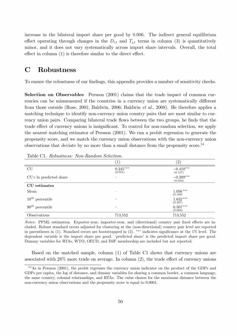
increase in the bilateral import share per good by 0.006. The indirect general equilibrium

e¤ect operating through changes in the Di,t and Tj,t terms in column (3) is quantitatively

minor, and it does not vary systematically across import share intervals. Overall, the total

e¤ect in column (1) is therefore similar to the direct e¤ect.

C Robustness

To ensure the robustness of our …ndings, this appendix provides a number of sensitivity checks.

Selection on Observables Persson (2001) claims that the trade impact of common cur-

rencies can be mismeasured if the countries in a currency union are systematically di¤erent

from those outside (Rose, 2001; Baldwin, 2006; Baldwin et al., 2008). He therefore applies a

matching technique to identify non-currency union country pairs that are most similar to cur-

rency union pairs. Comparing bilateral trade ‡ows between the two groups, he …nds that the

trade e¤ect of currency unions is insigni…cant. To control for non-random selection, we apply

the nearest matching estimator of Persson (2001). We run a probit regression to generate the

propensity score, and we match the currency union observations with the non-currency union

observations that deviate by no more than a small distance from the propensity score.54

Table C1. Robustness: Non-Random Selection.(1) (2)

CU 0.245(0.051)

¤¤¤ ¡0.410(0.157)

¤¤¤

CU£ ln predicted share – ¡0.209(0.044)

¤¤¤

CU estimates

Mean – 1.056(0.169)

¤¤¤

10th percentile – 1.632(0.287)

¤¤¤

90th percentile – 0.507(0.069)

¤¤¤

Observations 713,552 713,552

Notes: PPML estimation. Exporter-year, importer-year, and (directional) country pair …xed e¤ects are in-cluded. Robust standard errors adjusted for clustering at the (non-directional) country pair level are reportedin parentheses in (1). Standard errors are bootstrapped in (2). ¤¤¤ indicates signi…cance at the 1% level. Thedependent variable is the import share per good. ‘predicted share’ is the predicted import share per good.Dummy variables for RTAs, WTO, OECD, and IMF membership are included but not reported.

Based on the matched sample, column (1) of Table C1 shows that currency unions are

associated with 28% more trade on average. In column (2), the trade e¤ect of currency unions

54As in Persson (2001), the probit regresses the currency union indicator on the product of the GDPs andGDPs per capita, the log of distance, and dummy variables for sharing a common border, a common language,the same country, colonial relationships, and RTAs. The value chosen for the maximum distance between thenon-currency union observations and the propensity score is equal to 0.0001.

50

is heterogeneous across predicted import shares. Our …ndings thus remain robust to non-

random selection on observables.

Geopolitical Events, Decolonisation, and Missing Data Campbell (2013) and Camp-

bell and Chentsov (2020) argue that omitted variables and missing data are driving the positive

e¤ect of currency unions on trade. First, they argue that the collapse in trade attributed to

several currency union dissolutions was driven by major geopolitical events or hostile colonial

separations.55 Second, to account for the slow and steady decline of former colonial trade ties

over time (Head et al., 2010), they include a time trend for bilateral colonial relationships and

show that it signi…cantly reduces the trade impact of currency unions. Finally, as trade data

are often missing after currency union breakups, they recommend excluding those country pairs

from the sample as they may otherwise bias currency union estimates.

Table C2. Robustness: Geopolitical Events, Decolonisation, and Missing Data.(1) (2) (3) (4) (5) (6)

CU 0.173(0.050)

¤¤¤ 0.134(0.049)

¤¤¤ 0.135(0.049)

¤¤¤ ¡0.400(0.139)

¤¤¤ ¡0.417(0.135)

¤¤¤ ¡0.419(0.132)

¤¤¤

CU£ ln predicted share – – – ¡0.179(0.033)

¤¤¤ ¡0.179(0.037)

¤¤¤ ¡0.180(0.034)

¤¤¤

Trend colonial relationships ¡0.023(0.002)

¤¤¤ ¡0.022(0.002)

¤¤¤ ¡0.022(0.002)

¤¤¤ ¡0.022(0.002)

¤¤¤ ¡0.022(0.002)

¤¤¤ ¡0.022(0.003)

¤¤¤

CU estimates

Mean – – – 0.841(0.123)

¤¤¤ 0.824(0.143)

¤¤¤ 0.831(0.128)

¤¤¤

10th percentile – – – 1.320(0.205)

¤¤¤ 1.297(0.237)

¤¤¤ 1.307(0.214)

¤¤¤

90th percentile – – – 0.383(0.064)

¤¤¤ 0.366(0.065)

¤¤¤ 0.370(0.059)

¤¤¤

Observations 1,131,641 1,127,743 1,126,275 1,131,641 1,127,743 1,126,275

Geopolitical events Yes No No Yes No No

Hostile colonial separations Yes No No Yes No No

Missing data after CU switch Yes Yes No Yes Yes No

Notes: PPML estimation. Exporter-year, importer-year, and (directional) country pair …xed e¤ects are in-cluded. Robust standard errors adjusted for clustering at the (non-directional) country pair level are reportedin parentheses in (1) to (3). Bootstrapped standard errors in (4) to (6). ¤¤¤ indicates signi…cance at the 1%level. The dependent variable is the import share per good. ‘predicted share’ is the predicted import share pergood. Dummy variables for RTAs, WTO, OECD, and IMF membership are included but not reported.

To address those issues, in column (1) of Table C2 we estimate equation (6) and add a

time trend for past colonial relationships.56 Column (2) removes 32 (non-directional) country

pairs from the sample whose currency union switches were simultaneous to wars or hostile

colonial breakups, while column (3) also excludes 18 country pairs with missing data following

a currency union dissolution (Campbell, 2013; Campbell and Chentsov, 2020).57 The negative

55Examples include the breakup in 1965 of the currency union between India and Pakistan that coincidedwith a border war, or decolonisation after major con‡icts of former French and Portuguese colonies.

56The results are similar with a trend for UK colonies only (Campbell, 2013; Campbell and Chentsov, 2020).57Due to the country pair …xed e¤ects, we cannot separately control for these pairs in the regression. We

therefore follow Campbell (2013) and Campbell and Chentsov (2020) and remove them from the sample.

51

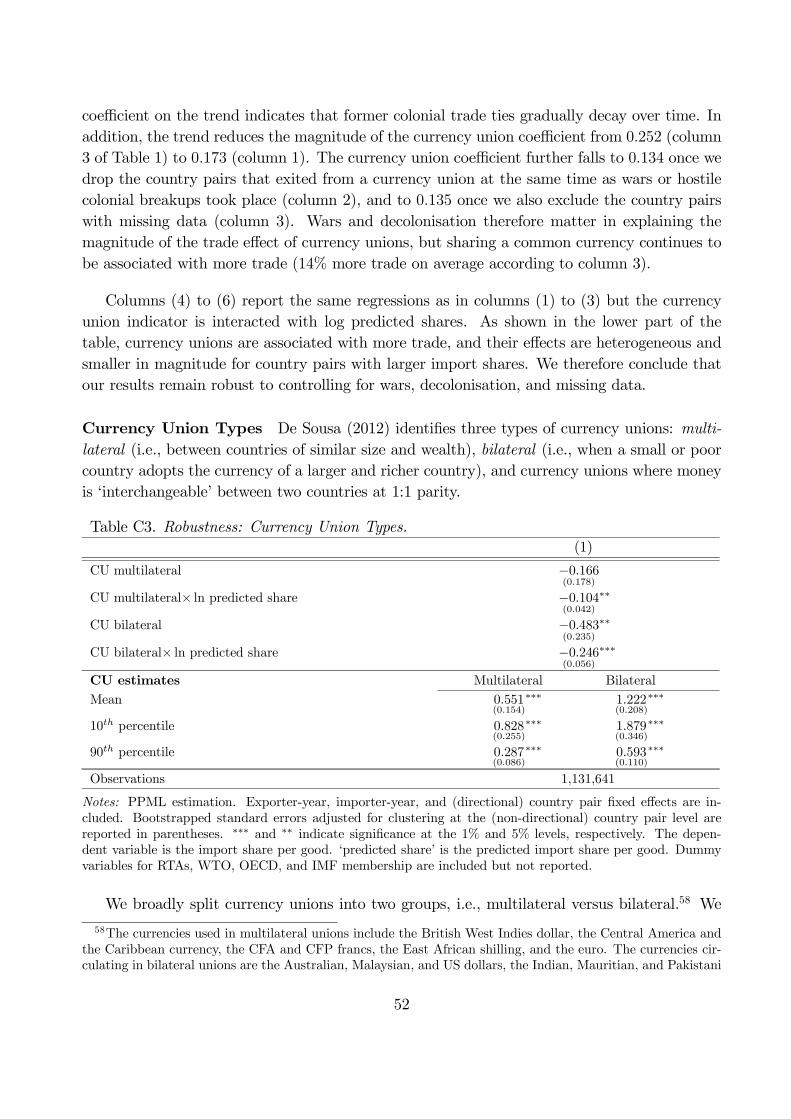
coe¢cient on the trend indicates that former colonial trade ties gradually decay over time. In

addition, the trend reduces the magnitude of the currency union coe¢cient from 0.252 (column

3 of Table 1) to 0.173 (column 1). The currency union coe¢cient further falls to 0.134 once we

drop the country pairs that exited from a currency union at the same time as wars or hostile

colonial breakups took place (column 2), and to 0.135 once we also exclude the country pairs

with missing data (column 3). Wars and decolonisation therefore matter in explaining the

magnitude of the trade e¤ect of currency unions, but sharing a common currency continues to

be associated with more trade (14% more trade on average according to column 3).

Columns (4) to (6) report the same regressions as in columns (1) to (3) but the currency

union indicator is interacted with log predicted shares. As shown in the lower part of the

table, currency unions are associated with more trade, and their e¤ects are heterogeneous and

smaller in magnitude for country pairs with larger import shares. We therefore conclude that

our results remain robust to controlling for wars, decolonisation, and missing data.

Currency Union Types De Sousa (2012) identi…es three types of currency unions: multi-

lateral (i.e., between countries of similar size and wealth), bilateral (i.e., when a small or poor

country adopts the currency of a larger and richer country), and currency unions where money

is ‘interchangeable’ between two countries at 1:1 parity.

Table C3. Robustness: Currency Union Types.(1)

CU multilateral ¡0.166(0.178)

CU multilateral£ ln predicted share ¡0.104(0.042)

¤¤

CU bilateral ¡0.483(0.235)

¤¤

CU bilateral£ ln predicted share ¡0.246(0.056)

¤¤¤

CU estimates Multilateral Bilateral

Mean 0.551(0.154)

¤¤¤ 1.222(0.208)

¤¤¤

10th percentile 0.828(0.255)

¤¤¤ 1.879(0.346)

¤¤¤

90th percentile 0.287(0.086)

¤¤¤ 0.593(0.110)

¤¤¤

Observations 1,131,641

Notes: PPML estimation. Exporter-year, importer-year, and (directional) country pair …xed e¤ects are in-cluded. Bootstrapped standard errors adjusted for clustering at the (non-directional) country pair level arereported in parentheses. ¤¤¤ and ¤¤ indicate signi…cance at the 1% and 5% levels, respectively. The depen-dent variable is the import share per good. ‘predicted share’ is the predicted import share per good. Dummyvariables for RTAs, WTO, OECD, and IMF membership are included but not reported.

We broadly split currency unions into two groups, i.e., multilateral versus bilateral.58 We

58The currencies used in multilateral unions include the British West Indies dollar, the Central America andthe Caribbean currency, the CFA and CFP francs, the East African shilling, and the euro. The currencies cir-culating in bilateral unions are the Australian, Malaysian, and US dollars, the Indian, Mauritian, and Pakistani

52

estimate equation (8) and allow for heterogeneity in the trade impact of both multilateral and

bilateral unions. For both types of unions, Table C3 shows that our results continue to hold.

Currency Union Entry and Exit Our sample includes 379 and 782 (directional) switches

into and out of currency unions. Among the 379 entries, 251 correspond to the euro.59 We

classify our currency union observations into three categories: entry (i.e., currency unions

created during our sample period), exit (i.e., unions that were dissolved), and continuous (i.e.,

they existed over the whole sample period). Some bilateral pairs are therefore classi…ed as both

entry and exit if they entered and subsequently left a currency union during our sample period.

Table C4. Robustness: Currency Union Entry and Exit.(1) (2)

CU entry ¡0.053(0.237)

–

CU entry£ ln predicted share ¡0.052(0.068)

–

CU non-EURO entry – ¡0.226(0.857)

CU non-EURO entry£ ln predicted share – ¡0.027(0.191)

EURO entry – ¡0.565(0.153)

¤¤¤

EURO entry£ ln predicted share – ¡0.118(0.036)

¤¤¤

CU exit ¡0.346(0.190)

¤ ¡0.238(0.183)

CU exit£ ln predicted share ¡0.204(0.044)

¤¤¤ ¡0.181(0.041)

¤¤¤

CU continuous£ ln predicted share ¡0.622(0.098)

¤¤¤ ¡0.630(0.088)

¤¤¤

Trend EU countries – 0.027(0.003)

¤¤¤

CU estimates Entry Exit Non-EURO entry EURO entry Exit

Mean 0.307(0.248)

1.064(0.160)

¤¤¤ ¡0.037(0.563)

0.250(0.129)

¤ 1.015(0.154)

¤¤¤

10th percentile 0.446(0.425)

1.607(0.265)

¤¤¤ 0.036(1.042)

0.564(0.219)

¤¤ 1.498(0.252)

¤¤¤

90th percentile 0.174(0.093)

¤ 0.544(0.090)

¤¤¤ ¡0.107(0.254)

¡0.051(0.066)

0.553(0.092)

¤¤¤

Observations 1,131,641 1,131,641

Notes: PPML estimation. Exporter-year, importer-year, and (directional) country pair …xed e¤ects are in-cluded. Bootstrapped standard errors adjusted for clustering at the (non-directional) country pair level arereported in parentheses. ¤¤¤, ¤¤, and ¤ indicate signi…cance at the 1%, 5%, and 10% levels, respectively. Thedependent variable is the import share per good. ‘predicted share’ is the predicted import share per good.Dummy variables for RTAs, WTO, OECD, and IMF membership are included but not reported.

Distinguishing between the three types of unions, we estimate equation (8) and report the

results in column (1) of Table C4 (for the continuous unions, the currency union dummy is

rupees, the Belgian and French francs, the South African rand, the Danish krone, the Portuguese escudo, theSaudi riyal, the Spanish peseta, and the British pound sterling.

59Belgium and Luxembourg are merged into a single entity, while Latvia and Lithuania only adopted the euroin 2014 and 2015. Our sample thus includes 16 countries that switched to the euro, accounting for 16£15 = 240directional switches. The 11 other switches occurred between Saint Pierre et Miquelon and Eurozone countries.

53

omitted due to collinearity with the pair …xed e¤ects and only its interaction with the log

predicted shares is included). The interactions between the currency union dummy and the log

predicted shares are negative for the continuous and exit unions only. In column (2), we split

the entry currency unions between euro and non-euro currencies (and include a trend for EU

countries), and the interaction is negative for the euro only. With the exception of non-euro

entry currency unions, all other unions are thus associated with heterogeneous trade e¤ects.

Import Shares per Good Our …ndings remain robust to using alternative proxies for the

extensive margin ni in measuring the bilateral import shares per good. In column (1) of Table

C5 the import shares per good are computed using the Hummels and Klenow (2005) measure.

In column (2) we assume that the extensive margin is unity for all exporters in which case the

dependent variable is simply the bilateral import share.

Table C5. Robustness: Import Shares per Good.(1) (2) (3) (4)

CU 0.180(0.165)

¡0.389(0.114)

¤¤¤ ¡0.704(0.447)

¡0.422(0.331)

CU£ ln predicted share ¡0.101(0.052)

¤ ¡0.186(0.028)

¤¤¤ ¡0.178(0.096)

¤ ¡0.178(0.096)

¤

CU estimates

Mean 0.771(0.182)

¤¤¤ 1.034(0.119)

¤¤¤ 0.736(0.353)

¤¤ 0.760(0.336)

¤¤

10th percentile 1.002(0.293)

¤¤¤ 1.647(0.205)

¤¤¤ 1.476(0.749)

¤¤ 1.499(0.724)

¤¤

90th percentile 0.542(0.094)

¤¤¤ 0.477(0.055)

¤¤¤ ¡0.086(0.135)

¡0.057(0.158)

Observations 854,082 1,157,168 81,807 100,301

Exporter extensive margin HK (2005) Unity Comtrade Comtrade

Importer output GDP GDP Total output Manuf. output

Notes: PPML estimation. Exporter-year, importer-year, and (directional) country pair …xed e¤ects are in-cluded. Bootstrapped standard errors adjusted for clustering at the (non-directional) country pair level arereported in parentheses. ¤¤¤, ¤¤, and ¤ indicate signi…cance at the 1%, 5%, and 10% levels, respectively. Thedependent variable is the import share per good. ‘predicted share’ is the predicted import share per good. In(1), HK (2005) stands for Hummels and Klenow (2005). Dummy variables for RTAs, IMF, OECD, and WTOmembership are included but not reported.

Instead of using the importing country’s GDP to compute the import shares per good, we

experiment using total (column 3) or manufacturing (column 4) gross output from the OECD

STAN database (available in domestic currency and converted to US dollars using bilateral

exchange rates from the International Monetary Fund’s International Financial Statistics). As

the data are only available for OECD nations our sample is reduced to 19 importing countries.

Speci…cations In Table C6 we consider three alternative speci…cations for the …rst-step

regression (7). In column (1), in addition to bilateral distance and contiguity we include

indicator variables for sharing a common language, a common coloniser post-1945, pairs in

a colonial relationship post-1945, and for territories that were, or are, the same country. In

54

column (2) we replace bilateral distance and contiguity with a full set of (directional) country

pair …xed e¤ects. In column (3) we let the distance and contiguity elasticities vary over time

(by interacting the two variables with year dummy variables).

In column (4) we include time-varying distance and contiguity controls in the second-step

regression (8). We also estimate the second-step regression with a lagged dependent variable

(column 5), a trend for EU countries (column 6), and a trend for all countries in a currency

union in our sample (column 7).

Table C6. Robustness: Speci…cations.

(1) (2) (3) (4) (5) (6) (7)

Lagged dep. var. – – – – 3.964(0.432)

¤¤¤ – –

CU ¡0.275(0.135)

¤¤ ¡0.240(0.139)

¤ ¡0.368(0.149)

¤¤ ¡0.335(0.151)

¤¤ ¡0.327(0.106)

¤¤¤ ¡0.498(0.143)

¤¤¤ ¡0.176(0.168)

CU£ ln predicted share ¡0.173(0.034)

¤¤¤ ¡0.173(0.037)

¤¤¤ ¡0.191(0.037)

¤¤¤ ¡0.188(0.035)

¤¤¤ ¡0.163(0.030)

¤¤¤ ¡0.201(0.034)

¤¤¤ ¡0.187(0.035)

¤¤¤

Trend EU countries – – – – – 0.021(0.003)

¤¤¤ –

Trend CU pairs – – – – – – ¡0.013(0.004)

¤¤¤

CU estimates

Mean 0.924(0.129)

¤¤¤ 1.104(0.177)

¤¤¤ 0.961(0.134)

¤¤¤ 0.965(0.125)

¤¤¤ 0.798(0.119)

¤¤¤ 0.892(0.130)

¤¤¤ 1.117(0.129)

¤¤¤

10th percentile 1.383(0.212)

¤¤¤ 1.742(0.310)

¤¤¤ 1.478(0.229)

¤¤¤ 1.465(0.212)

¤¤¤ 1.231(0.197)

¤¤¤ 1.427(0.214)

¤¤¤ 1.615(0.210)

¤¤¤

90th percentile 0.489(0.068)

¤¤¤ 0.528(0.075)

¤¤¤ 0.468(0.063)

¤¤¤ 0.485(0.067)

¤¤¤ 0.383(0.053)

¤¤¤ 0.379(0.070)

¤¤¤ 0.640(0.083)

¤¤¤

Observations 1,131,641 1,131,641 1,131,641 1,131,641 1,087,964 1,131,641 1,131,641

First-step controls Gravity Pair Dist.£Dt, Dist., Dist., Dist., Dist.,

controls e¤ects contig.£Dt contig. contig. contig. contig.

Notes: PPML estimation. Exporter-year, importer-year, and (directional) country pair …xed e¤ects are in-

cluded. Bootstrapped standard errors adjusted for clustering at the (non-directional) country pair level are

reported in parentheses. ¤¤¤, ¤¤, and ¤ indicate signi…cance at the 1%, 5%, and 10% levels, respectively. The

dependent variable is the import share per good. ‘predicted share’ is the predicted import share per good. In

(4), the second-step regression (8) includes time-varying distance and contiguity controls. Dummy variables for

RTAs, WTO, OECD, and IMF membership are included but not reported.

Samples In Table C7 we verify the robustness of our …ndings using alternative data samples.

In column (1) we use the exports and GDP data between 1949 and 2006 from Head et al. (2010).

In column (2) we use exports from the International Monetary Fund’s DOTS combined with

GDPs from the World Bank’s WDI between 1960 and 2013. In column (3) we use a balanced

sample between 1994 and 2013. We exclude (in column 4) the countries (mostly island nations)

omitted from the analysis of Glick and Rose (2016), smaller nations with a nominal GDP below

500 million US dollars in 2013 (column 5), poorer countries with an annual GDP per capita

below 500 US dollars in 2013 (column 6), and post-Soviet states (column 7).60

60The post-Soviet states are Armenia, Azerbaijan, Belarus, Estonia, Georgia, Kazakhstan, Kyrgyzstan,Latvia, Lithuania, Moldova, the Russian Federation, Tajikistan, Turkmenistan, Ukraine, and Uzbekistan.

55

Table C7. Robustness: Samples.(1) (2) (3) (4) (5) (6) (7)

CU ¡0.146(0.163)

¡0.360(0.135)

¤¤¤ ¡0.472(0.139)

¤¤¤ ¡0.394(0.157)

¤¤ ¡0.419(0.138)

¤¤¤ ¡0.485(0.135)

¤¤¤ ¡0.359(0.163)

¤¤

CU£ ln predicted share ¡0.130(0.038)

¤¤¤ ¡0.180(0.033)

¤¤¤ ¡0.156(0.039)

¤¤¤ ¡0.208(0.038)

¤¤¤ ¡0.195(0.035)

¤¤¤ ¡0.215(0.034)

¤¤¤ ¡0.195(0.040)

¤¤¤

CU estimates

Mean 0.768(0.133)

¤¤¤ 0.942(0.137)

¤¤¤ 0.547(0.133)

¤¤¤ 1.046(0.140)

¤¤¤ 0.933(0.127)

¤¤¤ 0.998(0.124)

¤¤¤ 0.990(0.138)

¤¤¤

10th percentile 1.117(0.229)

¤¤¤ 1.453(0.225)

¤¤¤ 0.934(0.224)

¤¤¤ 1.606(0.236)

¤¤¤ 1.445(0.212)

¤¤¤ 1.558(0.206)

¤¤¤ 1.511(0.239)

¤¤¤

90th percentile 0.432(0.065)

¤¤¤ 0.457(0.071)

¤¤¤ 0.180(0.061)

¤¤¤ 0.510(0.071)

¤¤¤ 0.439(0.061)

¤¤¤ 0.453(0.061)

¤¤¤ 0.490(0.062)

¤¤¤

Observations 986,961 970,993 310,080 992,368 1,102,783 1,012,463 1,053,636

Sample Head et al. IMF/World Balanced Excl. Excl. small Excl. poor Excl. Soviet

(2010) Bank 1994–2013 islands countries countries countries

Notes: PPML estimation. Exporter-year, importer-year, and (directional) country pair …xed e¤ects are included. Bootstrapped standard errors adjusted forclustering at the (non-directional) country pair level are reported in parentheses. ¤¤¤ and ¤¤ indicate signi…cance at the 1% and 5% levels, respectively. Thedependent variable is the import share per good. ‘predicted share’ is the predicted import share per good. Dummy variables for RTAs, WTO, OECD, and IMFmembership are included but not reported.

56

Feedback E¤ects Finally, in Table C8 we test for ‘feedback e¤ects’ of currency unions as

discussed in Baier and Bergstrand (2007). As in their paper, we restrict our sample to …ve-year

intervals from 1953 to 2013. Based on equation (8) we add one lead (i.e., values …ve years

ahead, denoted as t + 1) of the currency union dummy variable and its interaction with log

predicted shares. In column (1) we …rst show that our results continue to hold based on the

sample with …ve-year intervals. In column (2) we add the future currency union status and its

interaction with log predicted shares. These coe¢cients are insigni…cant. The coe¢cient on

the future currency union status remains insigni…cant in column (3) where we do not allow for

heterogeneity across country pairs. Similar to Baier and Bergstrand (2007) we therefore do not

…nd evidence of feedback e¤ects.

Table C8. Feedback E¤ects as in Baier and Bergstrand (2007).(1) (2) (3)

CU (t) ¡0.440(0.218)

¤¤ ¡0.356(0.317)

0.248(0.083)

¤¤¤

CU£ ln predicted share (t) ¡0.210(0.054)

¤¤¤ ¡0.180(0.082)

¤¤ –

CU (t+1) – 0.021(0.216)

0.047(0.069)

CU£ ln predicted share (t+1) – ¡0.014(0.052)

–

CU estimates (t)

Mean 1.001(0.175)

¤¤¤ 0.877(0.266)

¤¤¤ –

10th percentile 1.550(0.308)

¤¤¤ 1.345(0.475)

¤¤¤ –

90th percentile 0.472(0.075)

¤¤¤ 0.426(0.091)

¤¤¤ –

Observations 217,026 183,977 183,977

Notes: PPML estimation. Exporter-year, importer-year, and (directional) country pair …xed e¤ects are in-cluded. Bootstrapped standard errors adjusted for clustering at the (non-directional) country pair level arereported in parentheses in (1) and (2). Robust standard errors in (3). ¤¤¤ and ¤¤ indicate signi…cance at the1% and 5% levels, respectively. The dependent variable is the import share per good. ‘predicted share’ isthe predicted import share per good. Dummy variables for RTAs, WTO, OECD, and IMF membership areincluded but not reported.

57