grid code testing by voltage source...

Grid Code Testing by Voltage Source Converter

Master’s Thesis in the Master Degree Programme, Electric Power

Engineering

ABDULLAH AL MAHFAZUR RAHMAN

MUHAMMAD USMAN SABBIR

Department of Energy and Environment

Division of Electric Power Engineering

CHALMERS UNIVERSITY OF TECHNOLOGY

Göteborg, Sweden, 2012

Grid Code Testing by Voltage Source

Converter

by




CHALMERS UNIVERSITY OF TECHNOLOGY

Göteborg, Sweden

Master Thesis in ELECTRIC POWER ENGINEERING

Performed at: Chalmers University of Technology

SE-412 96 Göteborg,Sweden

Supervisor(s): Professor Ola Carlson

Examiner: Professor Ola Carlson


Chalmers University of Technology, SE-412 96 Göteborg

Grid Code Testing by Voltage Source Converter ABDULLAH AL MAHFAZUR RAHMAN


© ABDULLAH AL MAHFAZUR RAHMAN, 2012.

© MUHAMMAD USMAN SABBIR, 2012.


Chalmers University of Technology

SE-412 96 Göteborg

Sweden

Telephone + 46 (0)31-772 1000

Chalmers Reproservice

Göteborg, Sweden 2012

Grid Code Testing by Voltage Source Converter




Chalmers University of Technology

Abstract

The wind power penetration is increasing tremendously and according to EWEA that

wind will contribute up to 230 GW – 260 GW by 2020 in Europe and total wind power

generation in Europe would be 400 GW by 2030. To integrate this huge amount of

contribution from wind power into our current electrical system is a big challenge for

both power system planners and operators because of different behavior of wind power

plants than the conventional power plants. It is required from the wind power plants that

it should contribute in grid support such as frequency, voltage and reactive power control

and it should behave as a conventional power plant during normal and abnormal

conditions. For this reason transmission system operator’s (TSO) of different countries

have issued grid codes for wind power plants to operate them in conventional way.

In this project, a design of a voltage source converter (VSC) based test equipment has

proposed which can be capable to test a single wind turbine for the compliance of grid

codes to the wind turbine. The main objective to design this kind of test equipment is to

investigate the design and performance of a voltage source converter based test

equipment to test a single wind turbine and to set a base model for future discussions on

grid codes compliance to wind farms. The VSC based test equipment is found to be very

unique as it exhibits the characteristics of a grid and it can vary both frequency and

voltage independently. The most important factor that should be considered while

designing this kind of test equipment is the current and voltage ratings of the converter

and the maximum fault current provided by the wind turbine during short circuit test that

the equipment has to handle as this fault current can be several times higher than rated

current of wind turbine. It is also shown from simulation results that the test equipment

can be used successfully to verify the grid codes by creating different voltage and

frequency variations and can apply abrupt changes in voltage to exhibit short circuits

leading to voltage dips in the grid.

Keywords: Grid codes, voltage source converter, point of common coupling (PCC), fault ride through

capability.

Acknowledgement

We would like to take this opportunity to express our utmost appreciation and gratitude to our

thesis supervisor Professor Ola Carlson for his guidance and patience throughout the whole

thesis.

We would also like to thank to Massimo Bongiorno and Peiyuan Chen for their intuitive ideas

and guidance throughout this thesis work.

We would also like to thank to Stefan Ivarsson and Sara Janglund from GE Wind Energy for their

anticipation and support during this time.

Dedicated to our beloved parents

TABLE OF CONTENTS

Chapter 1 ....................................................................................................................................................... 1

Introduction ................................................................................................................................................... 1

1.1 History of Wind Energy .................................................................................................................. 1

1.2 Wind Energy Mechanism............................................................................................................... 2

1.3 Wind Power Plant Components .................................................................................................... 3

1.4 Development in Wind Energy........................................................................................................ 5

1.5 Offshore Wind Energy ................................................................................................................... 6

1.6 Grid Management ......................................................................................................................... 7

1.7 Thesis Objective ............................................................................................................................ 7

1.8 Structure of Thesis ......................................................................................................................... 7

Chapter 2 ....................................................................................................................................................... 9

Wind Turbine Architectures .......................................................................................................................... 9

2.1 Fixed Speed Wind Turbines ............................................................................................................... 9

2.2 Variable Speed Wind Turbines ......................................................................................................10

2.2.1. Doubly Fed Induction Generator Wind Turbine ..................................................................10

2.2.2. Fully Rated Converter Wind Turbine ...................................................................................11

2.3 Wind Turbine sizes .........................................................................................................................12

Chapter 3 .....................................................................................................................................................13

Voltage Source Converters ..........................................................................................................................13

3.1 Voltage source and Current source converter ............................................................................13

3.2 Single phase half bridge Voltage Source Inverter .......................................................................14

3.3 Single phase full bridge voltage source inverter .........................................................................14

3.4 Three phase voltage source inverter ...........................................................................................15

3.5 Switching technique of voltage source inverter ..........................................................................16

3.5.1. PWM inverter ......................................................................................................................16

Chapter 4 .....................................................................................................................................................19

Grid Code Requirements for Wind Farms ...................................................................................................19

4.1 Voltage Control ................................................................................................................................20

4.1.1. Reactive Power Compensation Requirements ....................................................................20

4.1.2. Voltage Range ......................................................................................................................23

4.2 Frequency Control ..........................................................................................................................24

4.3 Features of voltage and frequency change requirements ................................................................25

4.4 Fault Ride through Capability ............................................................................................................26

4.5 Impact of unsuccessful re-closure .....................................................................................................28

Chapter 5 .....................................................................................................................................................31

Design and Control Strategy ........................................................................................................................31

5.1 Design procedure of the proposed test equipment ..........................................................................31

5.1.1. The control scheme of the VSI.............................................................................................32

5.1.2. The inverter size and DC link voltage ..................................................................................32

5.1.3. Design of the PWM block ....................................................................................................33

5.2 Filter Design .................................................................................................................................33

5.3 Transformer .................................................................................................................................34

5.4 Design of test object ....................................................................................................................34

5.4.1. Design principle ...................................................................................................................35

5.4.2. abc to dq Transformation ....................................................................................................36

5.4.3. Phase locked loop: ...............................................................................................................38

5.4.4. P-Q controller ......................................................................................................................39

5.4.5. Tuning of controller for the test object ...............................................................................40

5.4.6. Externally control current source ........................................................................................40

5.5 Control strategy for different Grid code profiles ........................................................................41

5.5.1. Complete representation of the system .............................................................................41

Chapter 6 .....................................................................................................................................................43

Results and Analysis ....................................................................................................................................43

Case 1: Applying Active power and Reactive power steps in the P-Q controller respectively. .............43

Case 2: Applying 0.7 p.u voltage dip from the Converter .......................................................................46

Case 3: Voltage Control at the PCC .........................................................................................................49

Case 4: Low voltage Ride through Simulation .........................................................................................52

Three phase fault .................................................................................................................................52

Two phase fault .................................................................................................................................. 56

Single phase fault ................................................................................................................................59

Case 5: Features of voltage and frequency change ................................................................................62

Conclusion ...................................................................................................................................................65

Future Work ................................................................................................................................................67

References ...................................................................................................................................................69

Chapter 1

Introduction Energy is the major driver in the development of a society. As the world is developing day by

day, ultimately we have to find new energy resources to fulfil the demand to carry on this

development of the society. We cannot completely rely on our current energy sources like

thermal, nuclear and hydro because the fuel reserves for these sources are declining rapidly and

their environmental effects are quite alarming for the society. There exists a solution to this

problem is to use renewable energy sources i.e. wave and tidal power, solar power and wind

power. Their contribution to meet the demand is quite modest till now because the major

disadvantages of these renewable energy sources are that they are quite expensive and less

flexible as compared to conventional power plants. But many governments tend to value the

benefits of renewable energy sources more than the conventional generating plants .Hence they

support the expansion of renewable energy sources in various ways which basically means to

overcome the disadvantages associated to them. Among the renewable energy sources, wind

power is the most effective one and it is growing more rapidly due to its advantages over the

other renewable energy sources i.e. there is a lot of technology available to harness it and

technology is quite developed .People are using wind power for hundreds of years and there

are also quite a large number of wind power companies in the world.

1.1 History of Wind Energy Wind power is being used by humans for hundreds of years. It is the evolution from the use of

simple light devices driven by aerodynamic drag forces to heavy, material intensive drag

devices. At first wind power was used to sail boats and later on this led to development of sail –

type wind mills. In the start windmills were made for grinding grains, pumping water and the

design was known as vertical axis system. Wind energy used to generate electricity for the first

time by Charles F. Brush in 1888. Paris – Dunn and Jacobs were the pioneer companies for small

electrical output wind turbines simply used modified propellers to drive d.c generators. In 1979,

the modern wind industry started when Danish manufacturers started producing wind

turbines. Although at that time they were small in size 20 – 30 KW but now with the passage of

time they have increased greatly up to 7 MW. Figure: 1.1 below represents that how wind

power development took place from simple grinding speed or driving machines to wind parks

[1].

1

Figure: 1.1 Development of Wind parks.

1.2 Wind Energy Mechanism The sun does not heat the earth in an evenly manner such that the poles get less heat than the

equator and moreover dry land gets heat up and cool down more quickly rather than sea.

Therefore, some patches gets warmer than others rise, air blows in to replace them and we feel

blowing wind. We can say that it is a form of solar energy as wind is produced by uneven

heating of sun. The basic mechanism of wind energy is that it converts the kinetic energy of

wind into mechanical power by using turbines. Wind turbines are available in different sizes

according to different power ratings. Its mechanism is opposite to fan that rotates to generate

wind while wind turbine itself rotates by the wind to produce kinetic energy. There are two

types of wind turbines,

(i) Horizontal Axis Wind Turbines

(ii) Vertical Axis Wind Turbines

Betz Law is used to calculate maximum amount of power that can be extracted from a wind

power plant. It gives the maximum theoretical power but the original power that is extracted

from generator is lower as there are some transformation losses from mechanical to electrical

energy. Currently the most effective power plants have efficiency of about 50% and now the

consideration is to make more cheaper, more reliable and more flexible wind power plants [1].

The power in the airflow is given by,

P�� = ��ρAν (1.1)

Where,

ρ = air density (approximately 1.225 kgm�)

2

A= swept area of rotor, m�

ν= upwind free wind speed, ms��

Equation (1.1) gives the power that is available in the wind but the original power transferred to

wind turbine rotor is reduce by the power coefficient, Cp.

�� = �� (1.2)

Betz limit defines the maximum value of Cp that a turbine cannot extract more than 59.3%

power from air. In real its value varies between 25% – 45%. [1]

The tip speed ratio λ is an important parameter while designing a wind turbine as it measures

that how fast blades rotate with the wind speed.

λ = �� = ⍵�� (1.3)

Where, λ = Tip speed ratio v"#�$% = Tip speed of the blades (m/s) v&�'$ = Wind speed (m/s) ω = angular velocity (rad/s) r = radius of the rotor (m)

1.3 Wind Power Plant Components Wind power plants can have different architectures of electrical systems. Components are

chosen with respect to generator type to make more efficient and reliable wind power plant [1].

(1) Generators: Wind power plants can be equipped with any type of generators whether it is ac

or dc as it can be complied with the power electronics to synchronise it with the grid.

Mechanical construction of synchronous and asynchronous generators is same. A generator

consists of two main components, a rotor and a stator. Rotor consists of permanent magnets or

windings that generate a magnetic field when current flows into the rotor. As the rotor rotates, a

rotating magnetic field arises. When this magnetic field moves into stator windings, voltage is

induced in these windings. Mostly generator generates alternating current. With every

revolution of rotor current and voltage changes its direction accordingly. There are different

kinds of generators and they are categorized in figure 1.2.

3

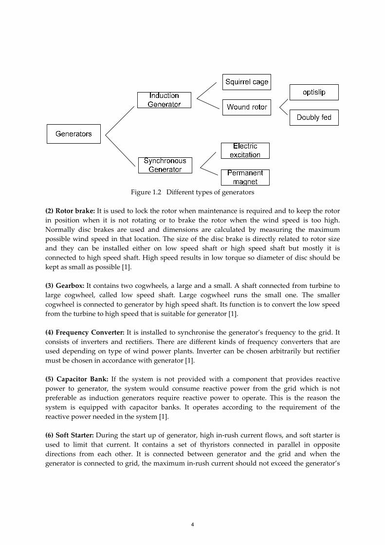
Figure 1.2 Different types of generators

(2) Rotor brake: It is used to lock the rotor when maintenance is required and to keep the rotor

in position when it is not rotating or to brake the rotor when the wind speed is too high.

Normally disc brakes are used and dimensions are calculated by measuring the maximum

possible wind speed in that location. The size of the disc brake is directly related to rotor size

and they can be installed either on low speed shaft or high speed shaft but mostly it is

connected to high speed shaft. High speed results in low torque so diameter of disc should be

kept as small as possible [1].

(3) Gearbox: It contains two cogwheels, a large and a small. A shaft connected from turbine to

large cogwheel, called low speed shaft. Large cogwheel runs the small one. The smaller

cogwheel is connected to generator by high speed shaft. Its function is to convert the low speed

from the turbine to high speed that is suitable for generator [1].

(4) Frequency Converter: It is installed to synchronise the generator’s frequency to the grid. It

consists of inverters and rectifiers. There are different kinds of frequency converters that are

used depending on type of wind power plants. Inverter can be chosen arbitrarily but rectifier

must be chosen in accordance with generator [1].

(5) Capacitor Bank: If the system is not provided with a component that provides reactive

power to generator, the system would consume reactive power from the grid which is not

preferable as induction generators require reactive power to operate. This is the reason the

system is equipped with capacitor banks. It operates according to the requirement of the

reactive power needed in the system [1].

(6) Soft Starter: During the start up of generator, high in-rush current flows, and soft starter is

used to limit that current. It contains a set of thyristors connected in parallel in opposite

directions from each other. It is connected between generator and the grid and when the

generator is connected to grid, the maximum in-rush current should not exceed the generator’s

4

nominal current. This current is about 6 to 8 times high than the rated current if there would be

no soft starter in the system [1].

1.4 Development in Wind Energy Wind energy growth in Europe has increased rapidly over the last few years. Almost 4.8% of

total energy consumption in Europe is provided by wind now days [8]. Main reason for this

rapid growth in Europe is that they are looking for a secure source of energy that is

independent of external source like oil and gas and the other factor is a major reduction in green

house emissions. Wind energy is playing a vital role as clean renewable resource and will

continue to play as emissions that are polluting atmosphere reduced tremendously.

Both these factors are the major reasons why Europe is more focused on this. Reason for wind

power that is expanding so rapidly is due to wind power technology that is evolved

significantly. Turbine size increased from 50 KV to more than 3 MW [19]. Rotor diameter has

also increased from 15 m to 100 m or more. Installation cost has also reduced with the time that

made it more attractive. Wind power capacity increased about 100 times in Europe over last

twelve years from 4753 MW in 1997 to 74767 MW in 2009 [8]. Almost 39% of all new electricity

that has been added to system is getting from wind can be seen in Table 1.2 .

European countries like Germany , Spain , Denmark , Italy , France , Portugal , Netherland ,

Sweden , Ireland , Greece and UK are playing the leading role in the development of world

wind energy technology. Among them Denmark, Spain, Portugal, Ireland and Germany have

managed more than 5% of total energy from the wind to meet their electricity demand [8]. As

the availability of wind energy resources varies from country to country and it will not be

equally important in all countries. There are some factors like ability of current transmission

networks and other generation plants to achieve large amount of wind energy considering the

strategic planning of wind farm development in the Europe.

Table 1.1 Top Ten Wind Power Countries [3]

Country Wind Power Capacity MW

China 44,733

United States 40,180

Germany 27,215

Spain 20,676

India 13,066

Italy 5,797

France 5,660

United Kingdom 5,204

Canada 4,008

Denmark 3,734

5

Table 1.2 Top Ten Electricity Generation European Countries [3]

1.5 Offshore Wind Energy Offshore wind energy has added more attraction in this sector due to less environmental effects

and truly speaking resources for wind energy generation are more than the centres of electricity

demand. At off shore, wind speeds are quite high so increased the energy production level

because wind speed is directly proportional to potential energy produced by wind by its cube

so a small increase in wind speed would make a significant change in energy output. The

average increase of wind energy at off shores is about 10 – 20 % [18].

Many countries have installed the off shore wind turbines to harness the wind energy of the

oceans to generate electricity as wind speeds on off shores are relatively much higher than on

shores. Many off shore areas have ideal conditions for wind energy production .Denmark and

UK have installed a number of off shore wind turbines to harness wind energy. Up till now just

600 MW of off shore wind energy is installed but now from 2010 it would be more than 11000

MW of which 500 MW each would be in United States and Canada and rest is in Europe and

Asia [18]. The development in offshore wind energy would be 22 % of total installed capacity in

Europe by 2020 and for around 12% in China. China is emerging rapidly in offshore industry

[1].

Country Wind Power Electricity Production

GWH

Spain 42,976

Germany 35,500

United Kingdom 11,440

France 96,00

Portugal 8,852

Denmark 7,808

Netherlands 3,972

Sweden 3,500

Ireland 3,473

Greece 2,200

Austria 21,00

6

1.6 Grid Management To integrate wind power plants to our current electrical system is a big challenge for both

power system planners and operators. This is due to the different behaviour of wind power

plants than the conventional plants. Wind power varies with the speed of wind and it cannot be

transmitted in a traditional way. Normally, induction generators are used for wind power

require reactive power for excitation and substations that are connected to the wind power

system have to include capacitor banks for power factor correction. Each wind turbine will

behave differently during grid disturbance so more dynamic modelling of wind farms is

required by TSO to ensure stability of system during faults.

1.7 Thesis Objective The main objective of the project is to develop a testing method for a single wind turbine by

using voltage source converter in order to make the grid codes compliance to the wind turbine

and to make wind turbines more efficient during normal and fault conditions in the grid. The

project will mainly work with the question that to what extent can a voltage source converter

can be used to test the grid codes for wind turbines. Project will carry out methods and

simulations for grid code tests with voltage source converters. The test object would be a full

power converter wind turbine.

A broad literature study will be done to clearly understand the dips and swells occurring in

grid voltage. Voltage dips would be created deliberately during the test by inducing a short

circuit in the grid side. Simulation of the complete testing system with the wind turbine and

voltage source converter will be done in PSCAD and then by creating different frequency and

voltage situations according to grid codes, their effect on the wind turbine will be investigated.

1.8 Structure of Thesis This thesis report consists of six chapters. Chapter 2 gives a brief description about different

types of wind turbines and their operating mechanisms and different sizes of wind turbines

available in the market.

Chapter 3 gives an understanding about voltage source converters and its different types.

Chapter 4 gives an overview of existing grid codes for wind farms issued by different

transmission system operators.

Chapter 5 describes the design and control strategy of the complete system i.e. test equipment,

test object, filter and transformer that has been designed in PSCAD.

Chapter 6 is about the simulation results. In this chapter results have been analysed and

summarised and then suggestions for future work has been presented.

7

Chapter 2

Wind Turbine Architectures

Large number of choices of architecture is available to wind turbine designers. For electricity

generation currently horizontal axis, three bladed, upwind turbines are normally used. Large

machines operates at variable speed while the small ones at constant or fixed speed. Modern

wind turbines are equipped with three blades upwind rotor while earlier two bladed and even

one bladed rotor were used commercially. By the reduction in number of blades now the rotor

has to rotate at higher speed to extract more power from the wind. Other important aspect is

that three bladed rotors are visually more attractive than the other designs that is also a reason

that now they are always used on large wind turbines [4].

Wind turbines are normally classified into two types,

• Fixed Speed Wind Turbines.

• Variable Speed Wind Turbines.

2.1 Fixed Speed Wind Turbines

Fixed speed wind turbines are electrically quite simple devices normally equipped with an

aerodynamic rotor that drives a low speed shaft, a gear box, a high speed shaft and an induction

generator (often called as asynchronous generator). In the electrical aspect they are considered

as large fan drives with torque applied to low speed shaft from the wind flow [4].

Soft starter

Squirrel cage induction generator

Capacitor bank

Turbine transformer

Figure 2.1 Schematic of a fixed-speed wind turbine

Figure 2.1 describes the working mechanism of fixed speed induction generator (FSIG)

configuration for wind generation. It consists of a squirrel cage induction generator connected

to grid by a turbine transformer. When the operating power level changes, the operating slip of

9

generator changes slightly with it. Although this variation is quite small i.e. less than 2% so it is

normally referred to as fixed speed.

As it is the characteristic of squirrel cage induction generator that it consumes reactive power so

it is obligatory to install capacitors at wind turbine for power factor improvement. The purpose

of soft starter is to create magnetic flux slowly and during energization of generator minimizes

transient currents [4].

2.2 Variable Speed Wind Turbines With the increase in size of wind turbines, the technology has moved from fixed speed to

variable speed. The purpose behind this transformation is to comply it with the grid codes

connection requirements and other advantage is the reduction in mechanical loads. Variable

speed wind turbines rely on pitch control rather than stall control. Rotor is allowed to speed up

with the wind gusts and thereby reducing the variations in active output power. Variable speed

wind turbines has many other advantages over fixed speed wind turbines like stress on

mechanical structure is reduced and the noise produced at low wind speeds would be less and

reactive power can be controlled at grid connection[4].

Most common variable speed wind turbines configurations are,

• Doubly Fed Induction Generator (DFIG) wind turbine.

• Full Rated Converter (FRC) wind turbine.

2.2.1. Doubly Fed Induction Generator Wind Turbine

The typical configuration of a DFIG is shown in figure 2.2

Figure 2.2 Typical configuration of DFIG wind turbine.

10

It uses a wound rotor induction generator with the slip rings to transmit current between

converter and rotor windings and to obtain a variable speed operation; a controlled voltage is

injected into the rotor at desired slip frequency. A variable frequency power converter based on

two AC/DC IGBT- based voltage source converters (VSCs), linked through a DC bus is used to

feed rotor winding. The variable frequency rotor supply from converter enables the rotor

mechanical speed to decouple from synchronous frequency of electrical network, so allows the

variable speed operation. The protection of generator and converters is done by voltage limits

and an over current crowbar. A DFIG wind turbine delivers the power to grid through both

stator and rotor. When the generator operates above the synchronous speed, the power will be

delivered from rotor through converters to the network. When the generator will operate below

synchronous speed then the rotor will absorb the power from the converter [4].

2.2.2. Fully Rated Converter Wind Turbine

Wind turbine manufacturers are now considering the induction or synchronous generators with

fully rated voltage source converters to give converter controlled, full power, variable speed

operation to fulfil present grid code requirements. The typical configuration of a full power

converter turbine is shown in figure 2.3,

Induction / Synchronous

generator

Figure 2.3 Typical configuration of fully rated converter-connected wind turbine.

This type of wind turbine may or may not have gearbox and wide range of electrical generators

can be employed such as asynchronous , conventional synchronous and permanent magnet .

Since all the power from the turbine goes to power converter, the specific characteristics and

dynamics of electrical generator are effectively isolated from power grid. Hence with the

variation in wind speed the electrical frequency of generator can vary but the grid frequency

remains same and hence allowing variable speed operation. Rating of power converter in this

type of wind turbine relates to rating of generator. There are many ways of arranging the power

converters. Generator side converter can be a diode rectifier or a voltage source converter while

11

the grid side converter is typically a Pulse width modulated VSC. The control scheme for the

operation of generator and power flowing to grid depends on converter arrangement. Torque

applied to generator is controlled by generator side converter while the grid side converter is

used to maintain the DC bus voltage or vice versa. Each of the converters has the ability to

absorb or generate the reactive power independently [4].

2.3 Wind Turbine sizes Turbine sizes are classified into three categories

(1) Utility Scale: The turbines in this category range from 900 KW to 2 MW per turbine. They

are used for generating bulk amount of power to sale in power markets. They are normally

installed in large wind energy projects but can also be used sometimes on small scale for

distribution lines [19].

(2) Industrial Scale: These are also called medium size turbines and normally range in between

50 KW to 250 KW. These are normally used in remote areas for grid production often in

conjunction with diesel generation [19].

(3) Residential Scale: These are very small scale turbines typically ranges in between 400 watts

to 50 KW and normally used for remote areas , for battery charging or net metering type

generation [19].

12

Chapter 3

Voltage Source Converters

Introduction

The power electronic converter process and controls the flow of electric energy by supplying

voltages and currents in a form that is optimally suited for the user loads. Due to better

controllability and improvement of semiconductor and microelectronic technology the use of

power electronic converters is increasing rapidly in domestic and industrial applications in the

last two decades .A power electronic converter consists of a power circuit which can be handled

by different types of switching pattern of power switches (GTO, MCT, BJT, MOSFET, IGBT) and

passive components (filter, shunt capacitor) and a control/protection system. Based on the type

of electrical subsystems the converters can be classified as AC to DC, DC to DC or DC to AC

converters [5]. A rectifier is a kind of converter where the average power flow of the circuit is

from the AC side to the DC of the converter. For the case of an inverter it is completely opposite

to the rectifier. But the bidirectional power flow in the system can be possible by the

implementation of specific classes of converters, where they can operate either as rectifier or

inverter, and this can be identified by the direction of load current that is connected with the

converter[5].

The following illustration describes the reasons of choosing voltage source inverter instead of

current source inverter in most of the High voltage direct current (HVDC) cases. Further, it

explains voltage source inverter (VSI) and its different types. Latter, it describes a bit about the

switching techniques of inverter.

3.1 Voltage source and Current source converter In conventional HVDC transmission system, current source converter (CSI) with line

commutation is implemented. A synchronous voltage source is needed to operate this type of

converters. The filters, series capacitors or shunt blocks, provide reactive power support in the

converter station during conversion process. If there is any kind of variation in reactive power

the ac source is responsible to adjust it. Reactive power variation needs to be kept small, to

maintain the ac voltage within the acceptable limit .The weaker the system or the further away

from generation, the tighter the reactive power exchange and must have to stay within the

desired voltage tolerance [6]. To hold the ac voltage within a fairly tight and acceptable range,

13

proper control and associated reactive power support is needed from the converter. The

conventional HVDC converters cannot bear much dynamic voltage support to the ac network

like a generator or static var compensator (SVC). Using Voltage source converter in HVDC

conversion technology can provide control over the power flow and at the same time it can also

provide dynamic voltage regulation to the ac system [6].

3.2 Single phase half bridge Voltage Source Inverter Figure.3.1 shows a half-bridge voltage source inverter, where two capacitors are connected in

series in such a way that they can share the dc link voltage equally, i.e. *�� . Assume the

capacitors are large enough to provide the constant voltage at point O with respect to the

negative dc bus N. During the ON stage of upper switch T1, the direction of current io decides

whether to conduct T1 or D1.This current is equally distributed through the two capacitors C1

and C2. Similarly the current io decides the conduction of T2 or D2, when the switch T2 is in

ON state. As the current have to flow through the capacitor C1 and C2 in the steady state, io can

not have any dc component. Thus the capacitors are acting as dc blocking capacitors [7].

Figure 3.1 Half bridge inverter

3.3 Single phase full bridge voltage source inverter

The circuit arrangement of a full power converter is shown in figure 3.2. From the figure it is

clearly seen that a full bridge converter is the composition of two half bridge converters. The

maximum output voltage of this converter is double that of half bridge converter with same

input, i.e. Vd [7].

14

Figure 3.2 Single phase full bridge inverter

3.4 Three phase voltage source inverter The most commonly used three phase inverter circuit consists of three legs, one for each phase

(conducts for120°), as shown in figure 3.3. Each inverter leg of the three phase inverter can be

explained from the figure 3.3 separately. Where the inverter output voltage depends on the

switching state and current sign. Leg A of the converter consists of upper and lower power

devices T1 and T4, and reverses recovery diodes D1 and D4 [7].

Figure 3.3 Three phase voltage source inverter

15

When T1 is turn on, a voltage *�/� is applied to the load. If the load draws positive current, it

will flow through T1 and delivers energy to the load. Conversely, if the load current ia is

negative, the current flows back to the dc source through D1.

Similarly if T4 is on or T1 is off, a voltage - *�/� is applied to the load. If ia is positive, energy

returns back to the dc voltage source through D4. A negative current conducts T4 and provides

energy to the load.

So, the voltage of each leg switches between *�/� to -

*�/� , respectively. The other phases can be

explained in the similar way [7].

3.5 Switching technique of voltage source inverter There are basically to types of modulation techniques used for the switching of VSI, which are

• Pulse width modulation (PWM) inverter

• Square wave inverter

For the case of Pulse width modulated inverters, the input dc voltage is maintained constant in

magnitude. So, the ac output voltage magnitude and frequency are controlled by the PWM

section of the inverters.

In square wave inverter, the magnitude of the output voltage is controlled by varying the input

dc voltage, and the inverter has to control the frequency of the output voltage. The output ac

voltage in this case is similar to a square wave, and hence the inverter is called square wave

inverter. The control of the square wave inverter is simple .The switching loss of this type of

converter is less but significant energies of lower order harmonics and large distortions in

current wave need large low-pass filters. A controlled rectifier is needed to control the voltage,

which added some additional costs of the inverter. So this is one of the big reasons for choosing

PWM technique instead of square wave operation [7].

3.5.1. PWM inverter

In pulse width modulation technique a carrier signal V12��%� is compared with a control signal V123'4�3# to generate the switching pattern of the inverter. The control signal is basically a

sinusoidal signal and chosen carrier signal is a triangular signal of very high frequency

compared with the control signal chosen for VSI. The frequency of the modulation signal

defines the fundamental frequency of the desired output signal of the inverter and the

frequency of the carrier signal decides the switching frequency of the inverter switches [7]. For

the case of three-phase inverter a three phase controlled voltage signal is compared with the

carrier signal as shown in figure 3.5. In this case three phase voltages are separately compared

16

with same triangular carrier signal in three separate comparators. Each comparator output

generates the switching signal for the corresponding inverter leg.

The ratio of the control signal magnitude to that of the carrier wave is called modulation index m�.

56 = 7189:;<9=718><<?@< (3.1)

Where V123'4�3#the peak value of the control is signal and V12��%� is the peak value of the carrier

signal.

Figure 3.5 PWM Pattern

Considering the linear range of operation (m ≤ 1), the fundamental component of the output

voltage in one of the legs of the inverter is,

AV1B'C� = m� *�� (3.2)

So, the line to line rms voltage at the fundamental frequency can be written as

DVE�EF�GH = √√� AV1B'C�

= √�√�m�V$

≅ 0.612m�V$ (3.3)

17

If the value of modulation index ma is allowed to increase more than 1, then the control signal

peak value exceeds the peak value of the carrier signal and the PWM shifted to over modulation

range. After that it is allowed to increase the ma more then, the PWM will act as square wave

operation where the maximum line to line rms voltage is equal to 0.78Vd. More explanation

about modulation techniques can be found in[7].

18

Chapter 4

Grid Code Requirements for Wind Farms

Introduction

As the wind power penetration is increasing tremendously and according to EWEA that wind

will contribute up to 230GW – 265GW by 2020 in Europe of which 40GW-55GW would be

offshore and total wind power generation in Europe would be 400GW by 2030 [8].By expecting

this huge contribution it is also required that wind power should also contribute in grid support

such as frequency, voltage and reactive power control and it should behave as a conventional

power plant in normal and abnormal conditions as these generators has quite different physical

characteristics compared to synchronous generators used in conventional power plants. For this

reason, there is a need of some specified technical documentation that wind power plants

should meet and for this reason transmission system operators (TSO) of different countries has

issued grid codes for wind farms to operate them in a conventional way [9].

Grid codes are the technical specifications for defining the parameters of a power plant that it

has to fulfil to ensure proper functioning of electrical grid.

Grid code can be the collection of transmission code, distribution and metering code, operation

code and scheduling and dispatch code, data regulation code and all kinds of other aspects.

Following benefits can be achieved using grid codes for the system:

• The TSO can dispatch the power in a safe way regardless of the generation technique.

• The number of project-specific technical negotiation with the TSO can be reduced.

• The wind turbine manufacturer can design their equipment knowing the requirements

properly and they will not need to change without warning or consultation.

Normally Grid code requirements are steady-state and dynamic active and reactive power

capability, continuously acting frequency and voltage control and fault ride-through (FRT)

capability.

In this chapter we have analysed grid code requirements for wind power generating units by

five different transmission system operators due to their great contribution in wind energy ,

(i) Svenska Kraftnät, Sweden [10]

(ii) E.ON Netz, Germany [11]

(iii) Energinet, Denmark [12]

19

(iv) National Grid Electricity Transmission plc, UK [13]

(v) ESB National Grid, Ireland [14]

Grid codes are divided into static and dynamic requirements. The static part relates to the

continuous operation of wind power plants and contains the requirements like voltage control,

quality of voltage, power factor requirements, power curtailment, frequency and flicker.

Dynamic part constitutes of the requirements regarding to operation of wind turbine during

faults and disturbances in grid i.e. fault ride through capability [15].

In this chapter we will discuss the most restringing conditions that we analysed in our thesis

work to give an idea about technical requirements that should be satisfied by a wind power

plant.

• Voltage control

• Frequency Control

• Fault Ride Through Capability

4.1 Voltage Control Voltage control is required in order to keep the voltage with in specific limits to get rid of

voltage stability issues. This can be achieved either by reactive power compensation or by using

automatic voltage regulator. In some grid codes it is made mandatory that wind farms should

be equipped with tap changing transformers [15].

4.1.1. Reactive Power Compensation Requirements

According to Svenska kraftnat [10], wind farms should be provided with automatic voltage

controller that can vary at least ±5% of nominal voltage. Reactive power compensation

requirements for this are shown in figure 4.1a which shows that reactive power exchange to the

system should be zero. It states that the wind power should have the ability of compensating

the reactive power requirement within the farm only nor for the grid [10].

Figure 4.1b shows the reactive power compensation for EnergiNet which states that 10 seconds

average reactive power exchange at common connection point must be able to withstand within

the control band. P-Q diagram showing the reactive power regulation must be provided by the

plant owner. It should be made clear for transmission system operator that how much reactive

power plant can take or supply to meet reactive power requirements [12].

20

Figure 4.1a Svenska KraftNat

Figure

Figure 4.1a Svenska KraftNat

Figure 4.1b EnergiNet

Figure 4.1a Svenska KraftNat.

EnergiNet.

.

21

Figure 4.1c E.ON

Figure 4.1d

Figure 4.1e ESBNG

Figure 4.1c E.ON

Figure 4.1d NGET

Figure 4.1e ESBNG

Figure 4.1c E.ON .

NGET.

Figure 4.1e ESBNG.

22

According to figure 4.1c and 4.1d for E.ON and NGET, the wind farm should be capable of

providing reactive power to the grid within that defined area [10] [13]. Figure 4.1e shows the

reactive power compensation requirements for ESBNG and unlike to others it applies its

requirements on low voltage side of grid connected transformer [14]. It can said that the reactive

power requirements by Svenska Kraftnat and EnergiNet are quite mild while to fulfil NGET

and ESBNG reactive power compensation requirements would be a challenge for wind power

industry to meet.

4.1.2. Voltage Range

Power system planners should make the system capable to run at a rated voltage in addition to

the specified voltage. This voltage range depends on the level of voltage on transmission line

and it varies from country to country. Table below shows the continuous operating voltage with

respect to nominal network voltage. Normal operation of wind power plants is only possible

within these specific limits and for particular time periods [15].

Table 4.1 Allowed Voltage Ranges[15]

Voltage Range

Germany Denmark UK

continuous -8% --->10%

-13---->12%

-13%-->12%

400KV

220KV

110KV

-10% --->5%

-3% --->13%

-5% --->10%

400KV

150KV

132KV

-10% --->5%

±10%

±10%

400KV

275KV

132KV

Limited

time

periods

X

-20% -->10%

-10% -->20%

-10% -->18%

400KV

150KV

132KV

±10%

±10%

±10%

400KV

275KV

132KV

While Svenska Kraftnat as compared to other grid codes has minimum requirements on voltage

deviations. The region of continuous operation varies from 90% to 105% of nominal voltage and

there will always be reduction in active power output outside from this region [10].

23

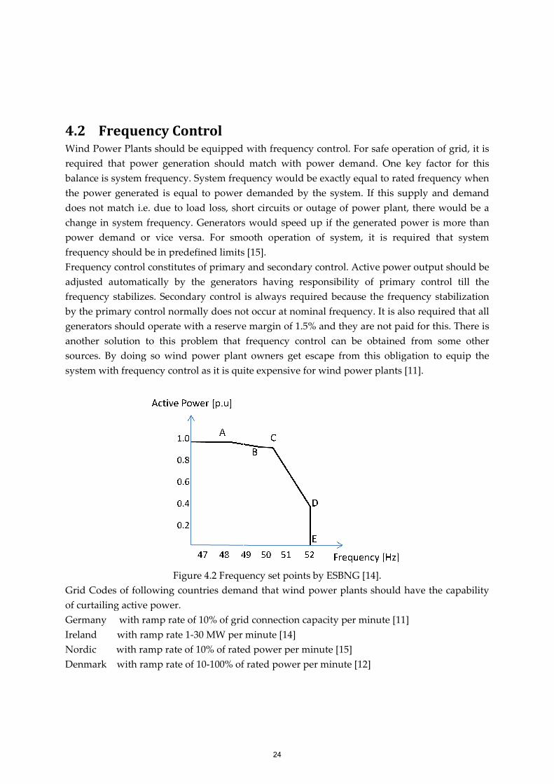
4.2 Frequency ControlWind Power Plants should be equipped with frequency control. For safe operation of grid, it is

required that power generation should match with power demand. One key factor fo

balance is system frequency. System frequency would be exactly equal to rated frequency when

the power generated is equal to power demanded by the system. If this supply and demand

does not match

change in system frequency. Generators would speed up if the generated power is more than

power demand or vice versa. For smooth operation of system, it is required that system

frequency should be in predefined limits

Frequency control constitutes of primary and secondary control. Active power output should be

adjusted automatically by the generators having responsibility of primary control till the

frequency stabilizes. Secondary control is always required because the freq

by the primary control normally does not occur at nominal frequency. It is also required that all

generators should operate with a reserve margin of 1.5% and they are not paid for this. There is

another solution to this problem that fre

sources. By doing so wind power plant owners get escape from this obligation to equip the

system with frequency control as it is quite expensive for wind power plants

Grid Codes of following countries demand that wind power plants should have the capability

of curtailing active power.

Germany with ramp rate of 10

Ireland

Nordic with ramp rate of 10% of rated power per minute [15]

Denmark with ramp rate of 10





does not match i.e.




uency control constitutes of primary and secondary control. Active power output should be











Ireland with ramp rate 1







i.e. due to load loss, short circuits or outage of po












Figure




with ramp rate 1-30 MW per minute [14]



4.2 Frequency Control Wind Power Plants should be equipped with frequency control. For safe operation of grid, it is




due to load loss, short circuits or outage of po












Figure 4.2 Frequency


Germany with ramp rate of 10% of grid connection capacity per minute [11]

30 MW per minute [14]


Denmark with ramp rate of 10-100% of rated power per

Wind Power Plants should be equipped with frequency control. For safe operation of grid, it is







frequency should be in predefined limits [15].






another solution to this problem that frequency control can be obtained from some other



4.2 Frequency set points by ESBNG


grid connection capacity per minute [11]



100% of rated power per













quency control can be obtained from some other



set points by ESBNG





100% of rated power per minute [





due to load loss, short circuits or outage of power plant, there would be a











set points by ESBNG [14].




minute [12]





wer plant, there would be a





frequency stabilizes. Secondary control is always required because the frequency stabilization





system with frequency control as it is quite expensive for wind power plants [11].




required that power generation should match with power demand. One key factor for this








uency stabilization







r this








uency stabilization






24

Table 4.2 Frequency Range Requirements[15]

Frequency Range

Frequency (Hz) Sweden Germany Denmark UK Ireland

52Hz to 53 Hz % % 3 min % %

51.5Hz to 52Hz 30 min % 30 min continuous 60 min

51Hz to51.5 Hz 30 min % 30 min continuous 60 min

50.5Hz to 51Hz Continuous continuous 30 min continuous 60 min

49.5Hz to

50.5Hz

Continuous continuous continuous continuous Continuous

49.5Hz to 47.5

Hz

Continuous continuous 30 min continuous 60 min

47.5Hz to 47Hz % % 3 min 20 sec 20 sec

4.3 Features of voltage and frequency change requirements The ability of the wind power unit to cope with variations in the grid voltage and frequency at

the connection point is described in the Grid Code SvK 2005:2 and is recalled in the Nordel

2007 grid code [16]. Although the Grid Code is planned for wind power plants but it can be

implemented in simulation model of single wind turbine.It can be explain from the figure4.3.

Figure:4.3 Voltage and frequency requirement in Nordel Nordic Grid Code[16]

25

Each of the rectangles of voltage and frequency has its own requirement for the wind power

unit to fulfill. The rectangles represented in the figure can be explained by the following way:

A. This condition represents the continuous operation mode. The wind power unit must be

able to operate within this range with no variations in the active and reactive power

capability [16].

B. In these operating conditions, the wind power unit shall be able to operate continuously

for at least 30 minutes. Active power reduction is allowed. In particular, the active

output power can decrease as a linear function of the frequency from zero (49 Hz) to

15% (47.5 Hz) [16].

C. In these operating conditions, the wind power unit shall be able to operate continuously

for at least 60 minutes. Active power reduction of 10% is allowed [16].

D. In these operating conditions, the wind power unit shall be able to operate continuously

for at least 60 minutes. Active power reduction of 10% is allowed [16].

E. In these operating conditions, the wind power unit shall be able to operate continuously

for at least 30 minutes. The Grid Code does not specify the percentage of reduction

allowed, but just mentions a “slight reduction” [16].

F. In these operating conditions, the wind power unit shall be able to operate continuously

for at least 3 minutes. Active power can be reduced at any level, but the wind power

unit must be able to remain connected [16].

4.4 Fault Ride through Capability With the increase in installed wind capacity in the transmission system makes it necessary that

wind generators should be connected to the system in case of network disturbance. Therefore

grid codes demand that wind farms should be able to withstand the voltage dips for specific

period of time and to a certain value of nominal voltage. Such a demand or requirement is

called Low voltage fault ride through or Fault Ride Through and it is shown by voltage versus

time characteristics. All countries have fault ride through capability figures and it is only

concerned with short circuit fault in transmission system not in the wind farm [15].

For the wind turbine generators to be connected to the transmission network, they should be

capable of providing active power in proportion to retain voltage and without exceeding the

generators limits must be capable to maximize the reactive current to transmission system in

case of voltage dips in transmission network.

Figure 4.3 represents the fault ride through requirements for Svenska Kraftnat. It has different

requirements for wind farm having rated active output power of 100MW and different for those

that varies in between 1.5MW and 100MW. Figure 4.3a with rated power of 100MW shows that

wind farm should remain connected to system during voltage dip down to zero voltage during

26

250ms and then increase linearly from 25% to 90% in 500ms. The wind farms with rated power

in the range of 1.5MW and 100MW requires that the wind farm should remain in contact with

the system during a voltage dip down to 25% and then there would be a step in voltage up to

90% at 250ms as shown in figure 4.3b [10].

Figure 4.3(b) SvK Fault Ride through Requirements.

27

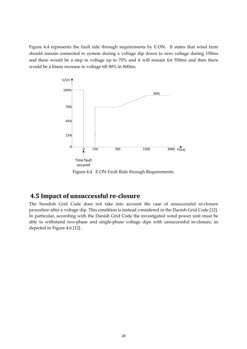
Figure 4.4 represents the fault ride through requirements by E.ON. It states that wind farm

should remain connected to system during a voltage dip down to zero voltage during 150ms

and there would be a step in voltage up to 70% and it will remain for 550ms and then there

would be a linear increase in voltage till 90% in 800ms.

0

15%

45%

100%

0 150 700 1500

U/Un

T(ms)

90%

Time fault

occured

3000

70%

Figure 4.4 E.ON Fault Ride through Requirements.

4.5 Impact of unsuccessful re-closure The Swedish Grid Code does not take into account the case of unsuccessful re-closure

procedure after a voltage dip. This condition is instead considered in the Danish Grid Code [12].

In particular, according with the Danish Grid Code the investigated wind power unit must be

able to withstand two-phase and single-phase voltage dips with unsuccessful re-closure, as

depicted in Figure 4.6 [12] .

28

Figure 4.6 (a)Two Phase fault and (b)Single Phase fault, according to Danish Grid Code.

29

Chapter 5

Design and Control Strategy

This chapter will give an overview of the design characteristics of proposed testing method for

the verification of grid codes for a single wind turbine. The test equipment consists of a voltage

source converter that typically behaves like a grid, connected to the test object i.e. a wind

turbine, through a low pass filter that consists of a capacitor and an inductor as shown in figure

5.1. The proposed test equipment is designed in PSCAD/EMTDC which is a powerful tool for

investigating the dynamic performance of power systems.

GRID

Figure 5.1 Single line diagram of proposed test equipment

It can be seen in the figure that proposed test equipment is connected to high voltage side of

transformer in order to reduce the current ratings of converter. Although this system is quite

expensive but it is more flexible as it depicts different grid characteristics for different short

circuit powers and can also be used for frequency and voltage variations and not only for

voltage dips but can also be used for voltage swells or over voltages.

5.1 Design procedure of the proposed test equipment There are different factors that needed to be considered during the design of test equipment.

The design is composed of different components and the following steps will describe them.

31

5.1.1. The control scheme of the VSI

The first step in the design is to gain control of the inverter. The inverter should be designed in

in such a way that it act as a grid for the test object. The grid should be totally independent from

the load. So for this project open loop control of the inverter is chosen, which can be seen from

the figure 5.2.

Figure 5.2 Open loop arrangement of the test equipment

5.1.2. The inverter size and DC link voltage

It is very important to select the current and voltage ratings of the inverter because the power

rating is determined from the maximum current and maximum voltage handled by device.

Generally, the valves of the power-electronic equipments are very sensitive to high currents as

compared to passive components [16]. To design the test equipment in PSCAD, the three phase

inverter arrangement has chosen, which is described in chapter 3 can be seen from the figure

5.3. The test equipment is designed for 50 kVA system which is quite simple to implement in

the lab. The DC link voltage of the converter is chosen as Vdc= 654 V, that is taken from a DC

voltage source.

Figure 5.3 General circuit diagram of the three phase voltage source inverter

32

5.1.3. Design of the PWM block

In this design scheme the output of the converter can be changed with the switching pattern of

the IGBT’s that can be achieved from the PWM block. For this two types of input is needed in

the PWM block. Firstly, a triangular signal, that acts as the carrier signal. Secondly, a three

phase signal, which will act as the control signal for the PWM block, as mention in the section

3.4. These two signals are compared in the comparator to generate the switching. The frequency

of the triangular signal is chosen as 1527 Hz, which represent the switching frequency of the

inverter. To get an output of 400 V line to line (rms) from the inverter with 50 Hz frequency, the

control signal is generated as 400 V line to line (rms) with 50 Hz. For this case the modulation

index is chosen as ma= 1 according to expression 3.3.

Figure 5.4 PWM signal generator

5.2 Filter Design The output of converter consists of number of harmonics that should be eliminated and for this

reason the filters are used. The main purpose of the filter is to eliminate the high frequency

harmonics that are generated by the switching of the valves of converter and to lessen the stress

on the valves of converter and wind turbine transformer as this filter connects the converter to

transformer. Reactance XL, of the filter is chosen as 0.2 p.u of ZBase of converter and having

internal resistance of 0.1 times of XL. The cut-off frequency of low pass filter is determined as,

w2N4�3OO = ��P√EQ (5.1)

In this project the cut-off frequency of LC filter that is connected at the output of converter is

chosen 10 times below the selected switching frequency. Switching frequency is chosen by

doing a trade off between quality of output voltage and losses.

33

5.3 Transformer In this project a built in model of transformer is used that is taken from PSCAD library. It

transfers the extracted power from wind to the grid by boosting the voltage level. In this project

a 1:1 transformer with the following parameters is selected,

Table 5.1 Parameters of Transformer

Transformer Parameters

Ratings

Transformer MVA

0.05 MVA

Operating Frequency

50 HZ

Primary Voltage

0.4 KV

Secondary Voltage

0.4 KV

Primary Winding Type

Y

Secondary Winding Type

Δ

Positive Sequence Reactance

0.1 P.U

No Load Losses

0

Copper Losses

0

5.4 Design of test object The test object of the system is a single wind turbine with back to back full power converters.

The wind turbine basically injects active power and as it is connected with the full power

converter it can exchange a certain amount of reactive power also.

The aim of the thesis is to test a wind turbine system through the designed VSI which should be

capable of providing the nature of grid. To design the test object is not the thesis goal. As there

is no built in model of the test object so for this project the test object is modelled in a simple

way but it should provide the similar types of effects as the conventional converter based wind

turbine. In wind turbine the generation of power varies with wind speed. But it is expected that

at the PCC the wind turbine should provide a fixed amount of power. If it is a full power

34

converter based wind turbine then the task is performed by the grid side converter. That means

the grid side converter try to inject the power at PCC in a controlled way. It means a reference

value of power at PCC have to be selected that the grid side converter should provide and the

converter tries to reach the task by its controllability. The P-Q controller based system can do

the things in the similar way. Where a reference value of power is selected and it tries to achieve

that by the help of its controller. For this case a P-Q controller based load has modelled. This can

exchange a given amount of real and reactive power at the point of common coupling. The

figure 5.5 shows the connection of load to the point of common coupling (PCC).

Figure 5.5 P-Q Controlled test object with PCC

5.4.1. Design principle

As it is mentioned in the earlier section that the load is P-Q controlled, it is needed to control the

active power and reactive power exchange at the point of common coupling (PCC). At the PCC

the voltage is to be maintained constant, so the power at that point can be controlled by

controlling the current through that point or vice verse. The design block is shown in figure 5.6.

35

Figure 5.6 Design of test object

5.4.2. abc to dq Transformation

It is the transformation of coordinates from three phase stationary coordinate system “abc” to

“dq” two phase rotating coordinate system. It is done in two steps,

(i) Transformation from three phase stationary coordinate system to two phase

stationary coordinate system known as"αβ", called Clark’s transformation.

(ii) Transformation from "αβ" to “dq” rotating coordinate system, called Park’s

transformation.

This transformation is done because in dq system the quantities are in dc form, so it is easy to

compare the dc quantity rather than ac. In dc system where frequency w=0,so integrator limit

goes towards infinite and it can make steady state error zero while in case of ac quantity the

integrator is limited to some value so it can reduce the steady state error to some value but

cannot make it to zero. So, it is easier to do analysis and control design tasks in “dq” coordinate

system [5].

Mathematically Clark’s transformation is expressed as,

Neglecting zero sequence v�DtF + v"DtF + v2DtF = 0

Where v�DtF, v"DtF, v2DtF are the three phase voltages,

36

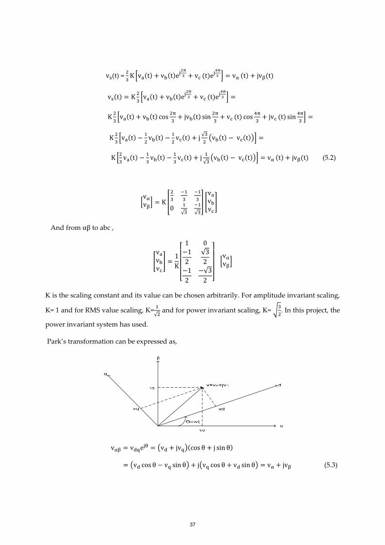
vH(t) =�K Yv�DtF + v"DtFe[\]̂ + v2DtFe[_]̂ ` = vaDtF + jvcDtF vHDtF = K � Yv�DtF + v"DtFe[\]̂ + v2DtFe[_]̂ ` =

K � Yv�DtF + v"DtF cos �P + jv"DtF sin �P + v2DtF cos hP + jv2DtF sin hP ` =

K � Yv�DtF − �� v"DtF − �� v2DtF + j √� Av"DtF −v2DtFC` =

K Y� v�DtF − � v"DtF − � v2DtF + j �√ Av"DtF −v2DtFC` = vaDtF + jvcDtF (5.2)

Yvavc` = K j� �� 0 �√ ��√

k lv�v"v2m And from αβ to abc ,

lv�v"v2m =1Knooop 1 0−12 √32−12 −√32 rs

sstYvavc`

K is the scaling constant and its value can be chosen arbitrarily. For amplitude invariant scaling,

K= 1 and for RMS value scaling, K=�√� and for power invariant scaling, K= u�. In this project, the

power invariant system has used.

Park’s transformation can be expressed as,

vac = v$ve[w = Av$ + jvvCDcos θ + j sin θF = Av$ cos θ − vv sin θC + jAvv cos θ + v$ sin θC = va + jvc (5.3)

37

Yvavc` = Ycos θ − sin θsin θ cos θ ` Yv$vv`

5.4.3. Phase locked loop:

Phase locked loop (PLL) is used to track angle of PCC voltage. PLL take the phase angle from

the PCC voltage and synchronizes the controller with that point. There are two types of PLL

used like voltage oriented PLL and flux oriented PLL. In voltage oriented PLL the voltage

vector is aligned with the d-axis that means the q-component of the voltage vector is equal to

zero. On the other hand, in flux oriented control the voltage vector is align with the q-axis that

means the d-component of the voltage vector is zero. For the case of drive’s control the flux

oriented PLL is used and for transmission and distribution of power the voltage oriented PLL is

used. As it is needed to sense the voltage at grid point, so the voltage oriented PLL is selected.

The figure 5.8 shows the block diagram and figure 5.9 shows the vector diagram of voltage

oriented PLL. The controller is voltage oriented, so PLL makes Vq=0, during steady state

operation it locks the controller phase voltage with the phase voltage of PCC.

Figure 5.7 Design of PLL block

The transfer function of the PI controller is, F2,�EE = k{,�EE + |�,}~~H (5.4)

The proportional gain kp,PLL=2α and the integrator gain ki,PLL=α2 taken from[17]. Where the

bandwidth α= 2πf�EE and f�EE is chosen as 5 Hz, as we are using slow PLL.

Figure 5.8 Voltage oriented PLL vector diagram

38

5.4.4. P-Q controller

To design the controller, the PI controller based system has selected. Because it is simple and the

voltage and current ratings are not the concerned here where in other types of controllers the

voltage needed to be scaled for a small value. As it is mentioned that the PLL is using here is

voltage oriented and the system is in power invariant, so the equations for active power and

reactive power in d-q frame are

P = v$i$ + vviv (5.5) Q = vvi$ − v$iv (5.6)

So if the d-component of the voltage is zero then the equations become P = v$i$ (5.7) Q = −v$iv (5.8)

Now from equation (5.7) and (5.8), if it is needed to make the voltage stagnant at PCC then only

by controlling the current, the active and reactive power can be controlled. The reference value

of the active power and reactive power are chosen and the actual value of the active and

reactive power can be measured from the PCC. Then these reference values and actual values of

the active power and reactive power are compared in separate comparators block to generate

the error signals. So when this error signal passes through PI controller it gives the current as

output. In figure 5.9 the voltage Vd is the D-component of PCC voltage that is measured and for

steady state operation this voltage is desired to be 1 p.u.

Figure 5.9 Block diagram of active power controller

For the active power controller the current,

i$ = DP�%O − PFF2 (5.9)

Where Fc is the transfer function of the PI controller. It can be written as,

Fc= �k{ + |�H � = k{ �1 + �� (5.10)

So from the equation 5.10, if the value of the proportional gain kp and the time constant of the

integrator Ts are known , then one can calculate the value of Fc.

In this case the value of the kp=0.97 is selected through hit and trial method .The value of time

constant Ts has chosen is 200ms.

39

Figure 5.10 Block diagram of reactive power controller

Same parameters are also used for the reactive power controller. In this case the current

equation is,

iv = −DQ�%O − QFF2 (5.11)

5.4.5. Tuning of controller for the test object

Initially the reference values for active and reactive power were set to zero then when a step to

the active power to 1 p.u is applied and the reactive power remains at zero, the actual value of

the active power try to reach its reference value and it takes 1.8 sec to settle with the reference

value. The rise time in this case is, trr= 500 ms.

Figure 5.11 Active power response

5.4.6. Externally control current source

It is a current source that consists of an external control and with high internal shunt impedance

chosen from PSCAD library. The outputs of the PI controller are converted from d-q quantity to

abc quantity and given it as the reference value of the current source.

Time [s] 0.0 1.0 2.0 3.0 4.0 5.0 6.0 7.0 8.0 9.0 10.0 1.5 2.0 0.5

-0.20

0.00

0.20

0.40

0.60

0.80

1.00

1.20

Act

ive P

ow

er

Curv

es

[p.u

]

0.104

0.910

0.807

Min 0.104

Max 0.910

Pref Pc

40

5.5 Control strategy for different Grid code profiles As it is mentioned earlier that the goal of this thesis project is to implement grid code test

through VSC, so VSC is modelled in such a way as shown in figure 5.15 that, it can satisfy the

requirements. It is know that by varying the amplitude of the control signal of PWM, the

magnitude of output voltage from the VSI will change. Similarly by varying the frequency of

the control signal the variation in the fundamental frequency of the output signal from the VSC

can be seen. In this project the similar technique has chosen. Grid code profiles for voltage

magnitude and frequency are created in p.u and multiplied them with the amplitude and

frequency of the control signals respectively. This provides the desired output from the VSC

that is applied to the test object.

Figure 5.12 Control strategy for different Grid code profiles

5.5.1. Complete representation of the system

Figure 5.13 represents the block diagram of complete model while figure 5.14 represents the

designed network in PSCAD with the components and its ratings.

41

Figure 5.13 Complete block Representation of the system

Figure 5.14 Complete design of the system in PSCAD

42

Chapter 6

Results and Analysis

In this chapter different simulation results are analysed by creating different voltage and

frequency profiles according to grid codes in order to see the response of the load in these

situations and to check the performance of designed test equipment in PSCAD. Project

considers different cases here and in each case voltage from converter is 1p.u and frequency is

set to 50 Hz.

Case 1: Applying Active power and Reactive power steps in the

P-Q controller respectively. The simulation is carried out in the following steps:

(i) Start with the initial condition and wait for some time until the system reaches steady

state.

(ii) At t=1.57 sec, set Pref= 1 p.u and Qref=0 p.u and wait to make the response stable.

(iii) At t=6.2sec, hold Pref to 1 p.u and set Qref to 1p.u and wait until response stabilized.

(iv) At t=9.1 sec, set Pref= 0 p.u and remain Qref to 1p.u and wait until the condition

stabilized.

(v) Finally at t= 12sec, hold Pref to 0 p.u and set Qref to 0 p.u.

The curves of the active and reactive power are seen form the figure 6.1(a) and (b) respectively.

The blue curves represent the reference value and the green curves represent the measured at

PCC. As both active and reactive power both are interrelated quantity, the step changes in one

gives the deviation in the value of other quantity. The measured values of both active power

and reactive power need some time to achieve the reference value.

Figure 6.1(a) Active Power Curves of the P-Q controller.

Time[s] 0.0 2.5 5.0 7.5 10.0 12.5 15.0 17.5 20.0

-0.20

0.00

0.20

0.40

0.60

0.80

1.00

1.20

Active P

ow

er

Curv

es

[p.u

]

Pref Pc

43

Figure 6.1(b) Reactive power curves of the P-Q controller

The current through the filter of the converter can be seen by the figure 6.2(a) and figure 6.2(b)

represents the 3-phase current output from the P-Q controller. Current from the controller will

increase when the active power step is applied, because at that time the voltage is fixed and the

active power depends only on the current injection from the current source. When P and Q

reference both are set to 1 p.u, the active and reactive current output from the P-Q controller

will increase. It is also noticeable that the current from the converter filter is also increased.

Figure 6.2 (a) 3-phase currents from the converter.

Figure 6.2 (b) 3-phase current from the P-Q controller.

Time[s] 0.0 2.5 5.0 7.5 10.0 12.5 15.0 17.5 20.0

-0.20

0.00

0.20

0.40

0.60

0.80

1.00

1.20

React

ive P

ow

er

Curv

es

[p.u

]

Qref Qc

Time[s] 0.0 2.5 5.0 7.5 10.0 12.5 15.0 17.5 20.0

-2.50

-2.00

-1.50

-1.00

-0.50

0.00

0.50

1.00

1.50

2.00

2.50

Cu

rre

nt

fro

m V

SC

[p

.u]

Ia1 Ib1 Ic1

Time[s] 0.0 2.5 5.0 7.5 10.0 12.5 15.0 17.5 20.0

-1.50

-1.00

-0.50

0.00

0.50

1.00

1.50

Cu

rre

nt

fro

m P

-Q c

on

tro

ller[

p.u

]

Ia Ib Ic

44

Figure 6.3(a) represents the control 3-Phase voltage given at the PWM of the converter. This is

considered as the reference voltage. The voltage measured at the point of common coupling

(PCC) can be seen from the figure 6.3(b). The PCC voltage is increased significantly when the

reactive power step is applied with the active power step.

Figure 6.3(a) 3-phase reference voltage

Figure 6.3(b) Voltage Measured at PCC

Time[s] 0.0 2.5 5.0 7.5 10.0 12.5 15.0 17.5 20.0

-1.50

-1.00

-0.50

0.00

0.50

1.00

1.50

Contr

ol V

oltage a

t P

WM

[p.u

]

Vref_A Vref_B Vref_C

Time[s] 0.0 2.5 5.0 7.5 10.0 12.5 15.0 17.5 20.0

-2.00

-1.50

-1.00

-0.50

0.00

0.50

1.00

1.50

2.00

PC

C v

oltages [

p.u

]

V_pccA V_pccB V_pccC

45

Case 2: Applying 0.7 p.u voltage dip from the Converter The simulation is carried out in following steps:

(i) Start with the initial condition and wait for some time until the system reaches steady

state. At t=1.65 sec, set Pref to 1 p.u and Qref remains to 0 p.u. Wait until the situation

reaches steady stare.

(ii) At t=3sec, holding the value of Pref and Qref, reduce the control signal magnitude to

30%, gives 0.7 p.u output from the converter. Wait for some time until the situation gets

stable.

(iii) At t=6 sec, apply a step on Qref to 0.5 p.u and wait for some time to see the response.

(iv) At t=9 sec, apply another step on Qref to 1p.u and wait until the situation get stable.

(v) Finally at t= 12 sec, bring back Qref to 0 p.u and voltage to 1 p.u values and wait for

some time until the system stabilized.

The active and reactive power curves are seen from figure 6.4(a) and 6.4(b) respectively, which

gives the similar kind of behaviour as in the previous case.

Figure 6.4 (a) Active power for 0.7p.u voltage dip.

Figure 6.4(b) Reactive power for 0.7p.u voltage dip.

The Control voltage for PWM, 3-phase Voltage for PCC and D-Q voltage for PCC at 0.7p.u

voltage dip are shown in figure 6.5 (a),(b) and (c) respectively. Form the effect of voltage dip is

seen clearly. As the reactive power steps are applied also in the simulation, it can be clearly seen

from the voltage curve at PCC. When the Qref is 1 p.u the voltage at PCC is maintained

Time[s] 4.0 6.0 8.0 10.0 12.0 14.0 16.0

-0.20

0.00

0.20

0.40

0.60

0.80

1.00

1.20

1.40

Active

Pow

er

Curv

es [

p.u

]

Pref Pc

Time[s] 4.0 6.0 8.0 10.0 12.0 14.0 16.0

-0.20

0.00

0.20

0.40

0.60

0.80

1.00

1.20

1.40

React

ive P

ow

er

Curv

es

[p.u

]

Qref Qc

46

approximately to 1 p.u. It means that if the reactive power support is applied, it is possible to

boost the voltage at PCC.

Figure 6.5 (a) Control voltage for PWM for 0.7p.u voltage dip

Figure 6.5(b) 3-phase Voltage for PCC for 0.7p.u voltage dip.

Figure 6.5(c) D-Q voltage of PCC for 0.7p.u voltage dip.

3-phase current from controller and from converter at 0.7p.u voltage dip are shown in figure 6.6

(a) and (b) respectively. Current is increased as the voltage is dropping down.

Time [s] 3.0 4.0 5.0 6.0 7.0 8.0 9.0 10.0 11.0 12.0

-1.50

-1.00

-0.50

0.00

0.50

1.00

1.50

Contr

ol vo

ltages

for

PW

M [

p.u

]


Time [s] 3.0 4.0 5.0 6.0 7.0 8.0 9.0 10.0 11.0 12.0

-1.50

-1.00

-0.50

0.00

0.50

1.00

1.50

3-p

hase

voltages

of

PC

C [

p.u

]


Time [s] 3.0 4.0 5.0 6.0 7.0 8.0 9.0 10.0 11.0 12.0

-2.00

-1.50

-1.00

-0.50

0.00

0.50

1.00

1.50

2.00

D-Q

voltages o

f P

CC

[p.u

]

V_d V_q

47

Figure 6.6(a) 3-phase current from controller for 0.7p.u voltage dip.

Figure 6.6(b) 3-phase current from converter at 0.7p.u voltage dip.

Time[s] 4.0 6.0 8.0 10.0 12.0 14.0

-2.00

-1.50

-1.00

-0.50

0.00

0.50

1.00

1.50

2.00 3-p

hase

Curr

ent

from

contr

olle

r[p.u

]

Ia Ib Ic

Time[s] 4.0 6.0 8.0 10.0 12.0 14.0

-3.0

-2.0

-1.0

0.0

1.0

2.0

3.0

3-p

hase

Curr

ent

from

conve

rter[

p.u

]

Ia1 Ib1 Ic1

48

Case 3: Voltage Control at the PCC To simulate this case, the grid codes compliance of Svenska Kraftnat is considered, which is

explained in section 4.1. For this simulation set the reactive power reference Qref to 0 p.u and

voltage from the converter is set to 1 p.u initially. Then change the voltage magnitude in to

some stapes like 1.05 p.u, 1p.u, 0.95 p.u and again to 1 p.u . On the other side vary the active

power reference Pref to 0.2 p.u, 0.4 p.u, 0.6 p.u, 0.8 p.u and 1 p.u at 2 sec, 6 sec, 10 sec, 14 sec and

18 sec respectively. The active power steps are shown in figure 6.7 (a)Active power.

Figure 6.7(a) Active power for case 3.

Figure 6.7(b) Reactive power curves for case 3.

During the time of simulation it is noticed that the voltage variation from the converter is given

to ±5% and the voltage at PCC gives the similar types of variation. This can be seen from figure

6.8(a) and (b) respectively.

Time[s] 0.0 2.5 5.0 7.5 10.0 12.5 15.0 17.5 20.0

-0.20

0.00

0.20

0.40

0.60

0.80

1.00

1.20

Act

ive

Po

we

r [p

.u]

Pref Pc

Time[s] 0.0 2.5 5.0 7.5 10.0 12.5 15.0 17.5 20.0

-0.010

0.000

0.010

0.020

0.030

0.040

0.050

Re

act

ive P

ow

er

[p.u

]

Qref Qc

49

Figure 6.8(a) 3-phase voltage for PWM in Case 3.

Figure 6.8(b) 3-phase Voltage at PCC for Case 3

As the active power is varied only and voltage variation very low, the current is increasing

significantly which can be seen from the figure 6.9.

Figure 6.9 (a)3-phase current from controller for case 3.

Time [s] 0.0 2.5 5.0 7.5 10.0 12.5 15.0 17.5 20.0

-1.25

-1.00

-0.75

-0.50

-0.25

0.00

0.25

0.50

0.75

1.00

1.25

3-p

ha

se v

olt

ag

es

for

PW

M[p

.u]


Time [s] 0.0 2.5 5.0 7.5 10.0 12.5 15.0 17.5 20.0

-1.25

-1.00

-0.75

-0.50

-0.25

0.00

0.25

0.50

0.75

1.00

1.25

3-p

ha

se v

olt

ag

es

at

PC

C [

p.u

]


Time[s] 0.0 2.5 5.0 7.5 10.0 12.5 15.0 17.5 20.0

-1.00

-0.75

-0.50

-0.25

0.00

0.25

0.50

0.75

1.00

3-p

hase C

urrent from

controlle

r [p

.u]

Ia Ib Ic

50

Figure 6.9(b) D-Q current from controller for case 3

Figure 6.9(c) 3-phase current from VSC for case 3.

Time[s] 0.0 2.5 5.0 7.5 10.0 12.5 15.0 17.5 20.0

-0.20

0.00

0.20

0.40

0.60

0.80

1.00

1.20

D-Q

Curr

ent

from

contr

oller

[p.u

]

Id Iq

Time[s] 0.0 2.5 5.0 7.5 10.0 12.5 15.0 17.5 20.0

-1.50

-1.00

-0.50

0.00

0.50

1.00

1.50

Curr

ent

from

VS

C [

p.u

]

Ia1 Ib1 Ic1

51

Case 4: Low voltage Ride through Simulation

Three phase fault

Low voltage ride through requirements are described in section 4.4.To simulate the three phase

fault the E.ON grid code profile is prepared in the simulation block as shown in figure 6.10. The

simulation is done in the following way:

(i) Start the simulation with Pref to 1 p.u and Qref to 0 p.u always.

(ii) 2. At t=0.2 set Pref=0.5 p.u and implement the E.ON grid code profile at that time.

Figure 6.10 E.ON’s Low voltage ride through profile applied in the converter

The Active Power and Reactive Power curves are shown in figure 6.11(a) and (b)

respectively. Before applying the profile the active power is reduced to 0.5 p.u, which is

shown in figure.

Figure 6.11(a) Active Power for three phase fault.

Time[s] 0.0 2.0 4.0 6.0 8.0 10.0

-0.40

-0.20

0.00

0.20

0.40

0.60

0.80

1.00

1.20

1.40

Voltage p

rofile

[p.u

]

a1

Time[s] 0.0 1.0 2.0 3.0 4.0 5.0 6.0 7.0 8.0 9.0 10.0

0.00

0.20

0.40

0.60

0.80

1.00

1.20

Act

ive

Po

we

r C

urv

es

[p.u

]

Pref Pc

52

Figure 6.11(b) Reactive Power curves for three phase fault.

The fault is applied from the converter side which is shown in figure 6.12(a). The effect of this

situation at the point of common coupling (PCC) can be seen from the voltage at PCC 6.12(b).

The d-component of the PCC voltage of figure 6.12(c) is quite similar to the profile of figure

6.10.

Figure 6.12(a) Control voltage for PWM for three phase fault.

Figure 6.12(b) 3-phase Voltage at PCC for three phase fault.

Time[s] 0.0 1.0 2.0 3.0 4.0 5.0 6.0 7.0 8.0 9.0 10.0

-0.100

-0.050

0.000

0.050

0.100

0.150

0.200

0.250 R

ea

ctiv

e P

ow

er

Cu

rve

s [p

.u]

Qref Qc

Time [s] 0.0 2.0 4.0 6.0 8.0 10.0

-1.50

-1.00

-0.50

0.00

0.50

1.00

1.50

Contr

ol V

oltages f

or

PW

M [

p.u

]


Time [s] 0.0 1.0 2.0 3.0 4.0 5.0 6.0 7.0 8.0 9.0 10.0

-2.00

-1.50

-1.00

-0.50

0.00

0.50

1.00

1.50

2.00

3-p

hase

volö

tage a

t P

CC

[p

.u]


53

Figure 6.12(c) D-Q voltage at PCC for three phase fault.

During the fault the voltage at PCC is decreasing and the current is increased very high as

shown in figure 6.13(a) 3-phase current from VSC,(b) 3-phase current from controller and (c)D-

Q current from controller.

Figure 6.13(a) 3-phase current from VSC for three phase fault.

Figure 6.13(b) 3-phase current from controller for three phase fault.

Time [s] 0.0 2.0 4.0 6.0 8.0 10.0

-1.00

-0.50

0.00

0.50

1.00

1.50

2.00

D-Q

voltage a

t P

CC

[p.u

]

V_d V_q

Time[s] 0.0 1.0 2.0 3.0 4.0 5.0 6.0 7.0 8.0 9.0 10.0

-2.50

-2.00

-1.50

-1.00

-0.50

0.00

0.50

1.00

1.50

2.00

3-p

hase C

urr

ent

from

VS

C [

p.u

]

Ia1 Ib1 Ic1

Time[s] 0.0 1.0 2.0 3.0 4.0 5.0 6.0 7.0 8.0 9.0 10.0

-1.25

-1.00

-0.75

-0.50

-0.25

0.00

0.25

0.50

0.75

1.00

1.25

3-p

hase

Curr

ent

from

contr

olle

r [p

.u]

Ib Ic Ia

54

Figure 6.13(c) D-Q current from controller for three phase fault.

Time[s] 0.0 1.0 2.0 3.0 4.0 5.0 6.0 7.0 8.0 9.0 10.0

-0.20

0.00

0.20

0.40

0.60

0.80

1.00

1.20

D-Q

Cu

rre

nt

from

con

tro

ller

[p.u

]

Id Iq

55

Two phase fault

The two phase fault and single phase fault is described in section 4.5 according to Danish grid

code. For two phase fault the grid code profile is prepared for simulation. The simulation is

done in the following way:

(i) Start the simulation with Pref=1 p.u and Qref to 0 p.u.

(ii) At t=0.2 sec apply Danish grid code profile for two phase fault.

The voltage of the corresponding phases goes to zero when the fault occurs on that phase.

This can be seen from the figure 6.14.

Figure 6.14(a) Control voltage for PWM for two phase fault.

Figure 6.14(b) 3-phase Voltage at PCC for two phase fault.

Time [s] 1.80 2.00 2.20 2.40 2.60 2.80 3.00 3.20 3.40 3.60

-2.00

-1.50

-1.00

-0.50

0.00

0.50

1.00

1.50

2.00

Contr

ol vo

ltages

of

PW

M [

p.u

]


Time [s] 1.80 2.00 2.20 2.40 2.60 2.80 3.00 3.20 3.40 3.60

-2.00

-1.50

-1.00

-0.50

0.00

0.50

1.00

1.50

2.00

3-p

hase

voltages o

f P

CC

[p.u

]


56

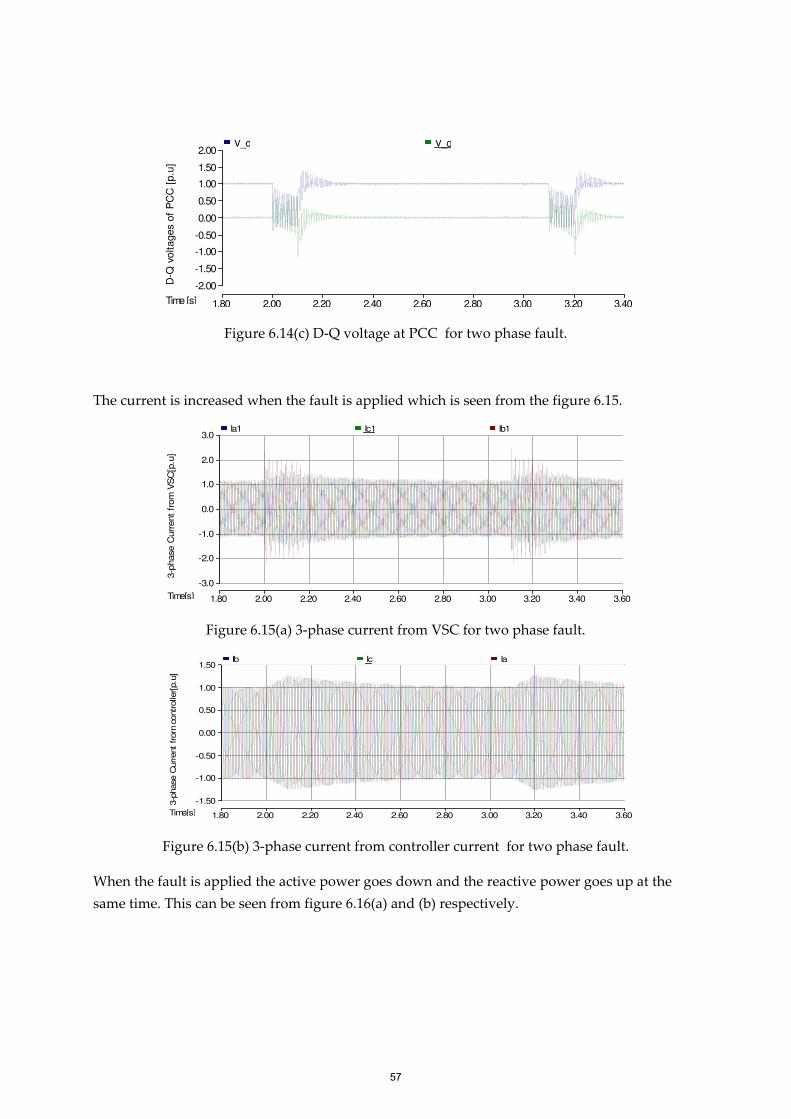
Figure 6.14(c) D-Q voltage at PCC for two phase fault.

The current is increased when the fault is applied which is seen from the figure 6.15.

Figure 6.15(a) 3-phase current from VSC for two phase fault.

Figure 6.15(b) 3-phase current from controller current for two phase fault.

When the fault is applied the active power goes down and the reactive power goes up at the

same time. This can be seen from figure 6.16(a) and (b) respectively.

Time [s] 1.80 2.00 2.20 2.40 2.60 2.80 3.00 3.20 3.40

-2.00

-1.50

-1.00

-0.50

0.00

0.50

1.00

1.50

2.00

D-Q

voltages

of

PC

C [

p.u

]

V_d V_q

Time[s] 1.80 2.00 2.20 2.40 2.60 2.80 3.00 3.20 3.40 3.60

-3.0

-2.0

-1.0

0.0

1.0

2.0

3.0

3-p

hase C

urr

ent

from

VS

C[p

.u]

Ia1 Ic1 Ib1

Time[s] 1.80 2.00 2.20 2.40 2.60 2.80 3.00 3.20 3.40 3.60

-1.50

-1.00

-0.50

0.00

0.50

1.00

1.50

3-p

hase

Current from

controlle

r[p.u

]

Ib Ic Ia

57

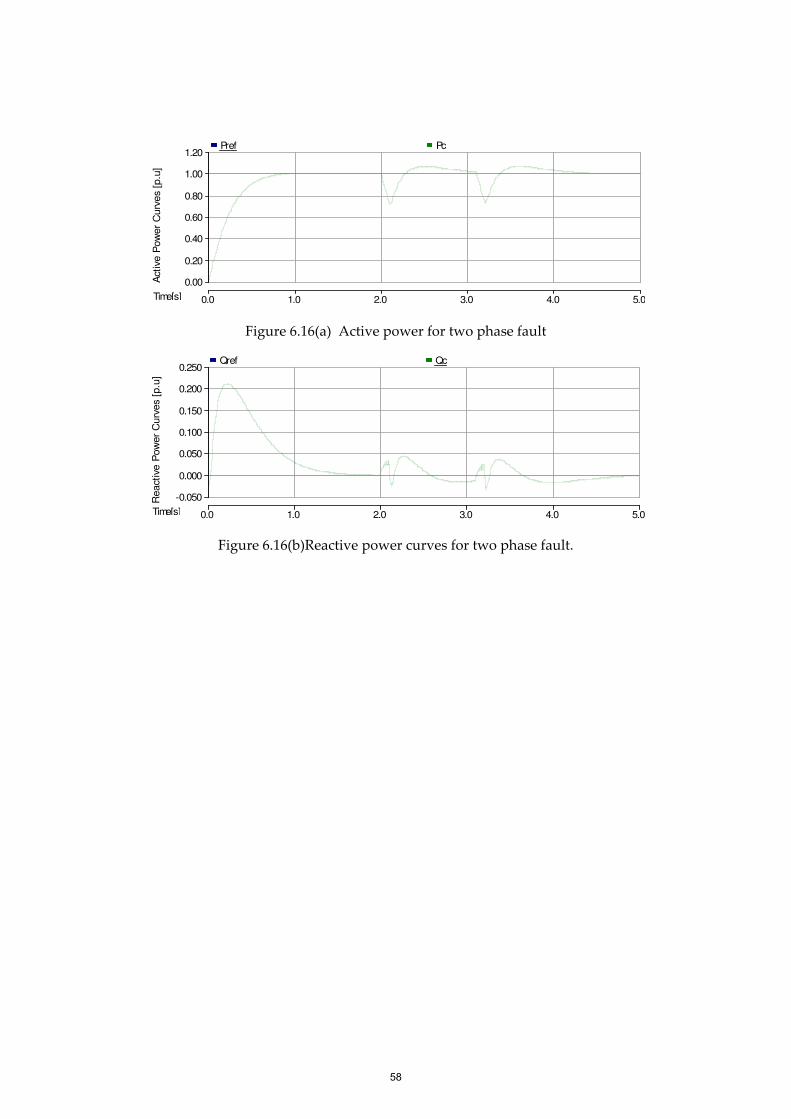
Figure 6.16(a) Active power for two phase fault

Figure 6.16(b)Reactive power curves for two phase fault.

Time[s] 0.0 1.0 2.0 3.0 4.0 5.0

0.00

0.20

0.40

0.60

0.80

1.00

1.20 A

ctiv

e P

ow

er

Curv

es

[p.u

]Pref Pc

Time[s] 0.0 1.0 2.0 3.0 4.0 5.0

-0.050

0.000

0.050

0.100

0.150

0.200

0.250

Reactive

Pow

er

Curv

es [

p.u

]

Qref Qc

58

Single phase fault

As mentioned in the previous simulation, this simulation is also performed by Danish grid

code profile for single phase fault, which is described in section 4.5. The simulation is

carried out in the following way:

(i) Start the simulation with Pref=1 p.u and Qref to 0 p.u.

(ii) At t=0.2 sec, apply the grid code profile .

The voltage of the phase A is goes to zero when the fault is applied in this phase, which is

shown in the figure 6.17(a).

Figure 6.17(a) Control voltage for PWM for single phase fault.

Figure 6.17(b) 3-phase Voltage at PCC for single phase fault.

Figure 6.17(c) D-Q voltage at PCC for single phase fault.

Time [s] 1.850 1.900 1.950 2.000 2.050 2.100 2.150 2.200 2.250 2.300 2.350

-1.50

-1.00

-0.50

0.00

0.50

1.00

1.50

Control voltages o

f PW

M [p.u

]


Time [s] 1.850 1.900 1.950 2.000 2.050 2.100 2.150 2.200 2.250 2.300 2.350

-1.50

-1.00

-0.50

0.00

0.50

1.00

1.50

D-Q

voltage a

t PC

C[p

.u]


Time [s] 1.850 1.900 1.950 2.000 2.050 2.100 2.150 2.200 2.250 2.300 2.350

-1.50

-1.00

-0.50

0.00

0.50

1.00

1.50

D-Q

voltage a

t PC

C[p

.u]

V_d V_q

59

The current from VSC and controller are shown in figure 6.18 (a) and (b) respectively. The

current is increased as fault occurs in the system.

Figure 6.18 (a) 3-phase current from VSC for single phase fault.

Figure 6.18(b) 3-phase current from controller current for single phase fault.

From the figure 6.19 of active and reactive power curve, shows clearly where the fault occurs.

Because during that time the active power at PCC is going down and the reactive power is

increased correspondingly.

Time[s] 1.950 2.000 2.050 2.100 2.150 2.200 2.250 2.300 2.350

-2.00

-1.50

-1.00

-0.50

0.00

0.50

1.00

1.50

2.00

3-p

hase

Curr

ent

from

VS

C[p

.u]

Ia1 Ic1 Ib1

Time[s] 1.950 2.000 2.050 2.100 2.150 2.200 2.250 2.300 2.350

-2.00

-1.50

-1.00

-0.50

0.00

0.50

1.00

1.50

2.00

Cu

rre

nt

fro

m c

on

tro

ller

[p.u

]

Ia Ib Ic

60

Figure 6.19(a) Active power for single phase fault.

Figure 6.19(b) Reactive power curves for single phase fault.

Time[s] 0.0 1.0 2.0 3.0 4.0 5.0

0.00

0.20

0.40

0.60

0.80

1.00

1.20 A

ctive

Pow

er

Curv

es [

p.u

]Pref Pc

Time[s] 0.0 1.0 2.0 3.0 4.0 5.0

-0.050

0.000

0.050

0.100

0.150

0.200

0.250

React

ive P

ow

er

Curv

es

[p.u

]

Qref Qc

61

Case 5: Features of voltage and frequency change In this case a frequency profile and a voltage as shown in figure 6.20(a) and (b) are prepared

according to the grid code described in section 4.3.This case only deal with the continuous

region A of the rectangle of figure 4.3 .The prepared profiles are implemented in the converter

three phase signal generator block, where the voltage profile is multiplied with the magnitude

of three phase signal and the frequency profile is multiply with the frequency of that signal to

provide the variation on voltage and frequency of the converter output respectively.

Figure 6.20 (a) Frequency profile .

Figure 6.20(b) Voltage profile.

The figure 6.21(a) 3-phase Voltages at PCC and (b) D-Q Voltage at PCC .The effect of voltage

variations can be seen from the figure. When the voltage from the converter side decreases or

vice-verse, similar types of response can be seen from the voltage at PCC.

Time[s] 0 100 200 300 400 500 600 700

48.50

48.75

49.00

49.25

49.50

49.75

50.00

50.25

50.50

50.75

Fre

quency

pro

file

[H

z]

freq3

Time[s] 0 100 200 300 400 500 600 700

0.850

0.900

0.950

1.000

1.050

Voltage p

rofile

[p.u

]

Dip3

62

Figure 6.21 (a) 3-phase Voltages at PCC .

Figure 6.21(b) D-Q Voltage at PCC.

The figure 6.22 (a) represents the 3-phase output Current from controller and 6.22(b) represents

the D-Q current through PCC. Observing the current curves it can be clearly seen that it behave

opposite to the voltage curves of figure 6.20.This is because to maintain constant power flow at

the PCC.

Figure 6.22 (a) 3-phase output Current from controller.

Time[s] 0 100 200 300 400 500 600 700

-2.00

-1.50

-1.00

-0.50

0.00

0.50

1.00

1.50

2.00

Vo

lta

ge

at

PC

C[p

.u]

V_pccB V_pccC V_pccA

Time[s] 0 100 200 300 400 500 600 700

-2.00

-1.50

-1.00

-0.50

0.00

0.50

1.00

1.50

2.00

D-Q

Vo

lta

ge

at

PC

C[p

.u]

V_d V_q

Time[s] 0 100 200 300 400 500 600 700

-1.50

-1.00

-0.50

0.00

0.50

1.00

1.50

3-p

hase

Curr

ent

from

contr

oller[

pu]

Ib Ia Ic

63

Figure 6.22(b)D-Q current through PCC.

From figure 6.23 the frequency variation and the respond from the test object can be observed.

The frequency is measured when the system is running with the frequency of 51.5Hz.At that

time the frequency of converter voltage and PCC voltage is measured and the result is found

approximately 51.5Hz.So the converter and the load is running with the same frequency which

is desired for stable operation of the system. It means that the PLL of the test object tracking the

converter frequency and the test object working at the same frequency as the converter.

Figure 6.23 Frequency measurements of the converter voltage and the PCC voltage.

Time[s] 0 100 200 300 400 500 600 700

-0.20

0.00

0.20

0.40

0.60

0.80

1.00

D-Q

curr

ent

from

contr

oller[

pu]

Id Iq

Time [s] 5.1400 5.1450 5.1500 5.1550 5.1600 5.1650 5.1700 5.1750 5.1800 5.1850 5.1519 5.1713 0.0194

-1.50

-1.00

-0.50

0.00

0.50

1.00

1.50

Control vo

ltages fo

r PW

M [p.u

] -0.837

-0.826

0.010

Min -1.000

Max 1.000


-2.00

-1.50

-1.00

-0.50

0.00

0.50

1.00

1.50

PCC voltages [p.u

]

-0.923

-0.912

0.012

Min -1.037

Max 1.025


64

Conclusion In this project, a testing method is developed which will be feasible for a single wind turbine to

test grid codes compliance by using voltage source converter based test equipment, so that the

wind turbines would become more efficient in normal and fault conditions in the grid. The test

equipment consists of a voltage source converter that exhibits the characteristics of a grid. In

practical case the test object will be a wind turbine connected to the grid through transformer

and transmission line. For the simplicity of modelling and analysis a P-Q controlled test object is

designed instead of the wind turbine. This kind of test object has the similar type of behaviour

like a wind turbine in active and reactive power exchange with the grid. From the simulation

results, it can be seen that different voltage and frequency variations can be applied to the test

equipment according to grid codes by the voltage source converter. Moreover voltage source

converter based test equipment can also provide the effect of fault on the grid side and from the

behaviour of test object, the behaviour of wind turbine can be estimated connected to the grid

during the faulty condition.

65

Future Work In this project, the whole system is implemented in PSCAD so one can realise the necessity to

perform a laboratory test/ a real time simulation test in order to verify the obtained results and

for different wind turbine topologies and wind conditions. This testing method is designed to

test a single wind turbine but as the current system consists of wind farms/parks so a testing

method can be designed to test a wind farm/park.

67

References

[1] Kristin Bruhn, Sofia Lorensson, Jennie Swenson,”Wind Power-A Renewable Energy

Source in Time”,2009.

[2] World Wind Energy Report 2010 . World Wind Energy Association Feb. 2011.

[3] Eolic Energy News 2010-12-31.

[4] Ake Larsson,”Power Quality of Wind Turbine Generating Systems and their interaction

with grid”.

[5] Amirnaser Yazdani, Reza Iravani,’’Voltage Source Converters in Power System’’, A John

Wiley and sons inc.,publication,2010.

[6] Michael P. Bahrman, Jan G. Johansson and Bo A. Nilsson, ‘’Voltage Source Converter

transmission Technology’’.

[7] N. Mohan, T.M. Undeland and W.P. Robbins ”Power Electronics: converter,

applications and design”, Media Enhanced third edition, 2002.

[8] EWEA.ORG

[9] Maria Paz Comech, Miguel Garcia, Susana Martin Arroy and Miguel Angel

MartinezGuillen,” Wind Farms and Grid Codes”.

[10] Business Agency Svenska KraftNat’s Regulations and general advice concerning design

of production plants 2005.

[11] E.ON Netz Grid Code High and Extra High Voltage 2006.

[12] Wind Turbines Connected to Grid with Voltages above 100 kv, Technical Regulations for

the properties and regulations of wind turbines.

[13] National Grid Electricity Transmission, Uk.

[14] Wind Farm Power Station Grid Codes. ESBNG , Ireland.

[15] Willi Christiansen and David T.Johansen, ”Analysis of requirements in selected grid

codes”.

[16] Massimo Bongiorno, Andreas Petersson, ’’Development of a Method for Evaluation of

Wind Turbines Ability to fulfil Swedish Grid Codes’’, Elforsk Repport, February, 2009.

[17] S. Islam K.Tan, “Optimum control strategies in energy conversion of PMSG wind

turbine system without mechanical sensors,” IEEE transaction on Energy conversion,

vol. 19, p. 392, June 2004.

[18] OCS Alternative Energy and Alternate Use Programmatic EIS.

[19] Wind Turbine Zone (Home to Wind Power Industry).

69

grid code testing by voltage source...

Documents