groundwater characterisation and disposal modelling for coal
TRANSCRIPT

GROUNDWATER CHARACTERISATION AND
DISPOSAL MODELLING FOR COAL SEAM
GAS RECOVERY
__________________________________
A thesis submitted in partial fulfilment of
the requirements for the Degree of PhD in
Environmental Engineering in the
University of Canterbury
by Mauricio Taulis
__________________________________
University of Canterbury
2007

i
Contents
Contents...........................................................................................................................i
List of Tables ................................................................................................................. iv
List of Figures ............................................................................................................... vi
Acknowledgements ........................................................................................................ix
Abstract ..........................................................................................................................1
Chapter 1 ........................................................................................................................3
General Introduction .................................................................................................................3 Objective ................................................................................................................................................3 Thesis outline .........................................................................................................................................4
Chapter 2 ........................................................................................................................5
Identification of Coal Seam Gas waters in New Zealand .......................................................5 Introduction............................................................................................................................................5 The genesis of coal seam gas .................................................................................................................6 Coal seam gas storage and migration...................................................................................................11 CSG mining procedure.........................................................................................................................14 Chemistry of waters associated with coal seam gas.............................................................................16
Dissolution of Sodium Feldspars ....................................................................................................17 Bicarbonate concentrations .............................................................................................................18 Calcium and Magnesium depletion with ion exchange. ..................................................................19 Sulphate reduction...........................................................................................................................20
Differences with Acid Mine Drainage (AMD) ....................................................................................22 CSG water quality from US basins ......................................................................................................24 CSG water quality from potential New Zealand basins .......................................................................31
Methods...........................................................................................................................................32 CSG exploration in New Zealand ...................................................................................................35
Discussion ............................................................................................................................................46 References............................................................................................................................................50
Chapter 3 ......................................................................................................................55
Coal Seam Gas Water Quality Variability ............................................................................55 Introduction..........................................................................................................................................55 Preliminary analysis of Maramarua data..............................................................................................55 Time series analysis of Maramarua data ..............................................................................................67 Multivariate analysis of Maramarua data.............................................................................................70
Maramarua CSG water quality data review for factor analysis.......................................................71 Factor analysis results .....................................................................................................................74 Discussion of factor analysis results ...............................................................................................78
Degassing investigation analysis..........................................................................................................85 Methods...........................................................................................................................................86
Practical experiment ...................................................................................................................86 Theoretical experiment ...............................................................................................................87
Experimental results........................................................................................................................87 Discussion of experimental results..................................................................................................90
Conclusion ...........................................................................................................................................94 References............................................................................................................................................96
Chapter 4 ......................................................................................................................97
Potential environmental impacts associated with coal seam gas water management in New Zealand .............................................................................................................................97
ii
Introduction..........................................................................................................................................97 Assessing environmental impacts related to CSG water management and disposal ............................98
Land disposal of CSG waters ..........................................................................................................99 Surface water disposal of CSG water............................................................................................108 Disposal alternatives and management options.............................................................................113
Case Study: Assessing the environmental effects of CSG water disposal in Maramarua ..................120 Site description..............................................................................................................................120 Maramarua CSG water..................................................................................................................124 Soil Sampling ................................................................................................................................124 Effects arising from land disposal of CSG waters.........................................................................127
Assessment of salinity hazard...................................................................................................127 Methods ...............................................................................................................................127 Results .................................................................................................................................129 Discussion............................................................................................................................131
Assessment of soil infiltration problems ..................................................................................132 Assessment of specific ion toxicity ..........................................................................................137
Effects arising from surface water disposal of CSG waters ..........................................................139 Potential effects on aquatic life ................................................................................................140 Potential effects on vegetation..................................................................................................141
Conclusions........................................................................................................................................143 References..........................................................................................................................................147
Chapter 5 .................................................................................................................... 152
Sodium removal from Maramarua coal seam gas waters using Ngakuru zeolites ..........152 Introduction........................................................................................................................................152 Materials and Methods.......................................................................................................................154
Materials........................................................................................................................................154 Methods.........................................................................................................................................158
Batch tests.................................................................................................................................158 Flow-through tests ....................................................................................................................162
Results................................................................................................................................................165 Batch test results ...........................................................................................................................165 Flow-through tests.........................................................................................................................173
Discussion ..........................................................................................................................................187 Batch tests .....................................................................................................................................187 Flow-through tests.........................................................................................................................192
Conclusion .........................................................................................................................................205 References..........................................................................................................................................209
Chapter 6 .................................................................................................................... 211
Conclusions .............................................................................................................................211
Appendix A ................................................................................................................. 216
A.1 Laboratory methods .................................................................................................216
A.2 CSG exploration in New Zealand .........................................................................218 A.2.1 Ashers-Waituna ...................................................................................................................218 A.2.2 Reefton ................................................................................................................................221 A.2.3 Kaitangata............................................................................................................................222 A.2.4 Hawkdun..............................................................................................................................225
A.3 Sample collection methods .......................................................................................233
A.4 References ..................................................................................................................238
Appendix B ................................................................................................................. 239
B.1 Sodium calculations and corrections.......................................................................239
B.2 Precision and accuracy .............................................................................................241

iii
B.3 Time plots for parameters ........................................................................................249
B.4 Principal components analysis .................................................................................252
B.5 Factor analysis...........................................................................................................256
B.6 Implementing Factor Analysis using MINITAB....................................................263
B.7 Data transformation for factor analysis..................................................................264
B.8 References ..................................................................................................................267
Appendix C ................................................................................................................. 269
C.1 Infiltration risk model ..............................................................................................269 Introduction........................................................................................................................................269 Materials and Methods.......................................................................................................................269 Results................................................................................................................................................271
C.2 Soil Salinity calculations...........................................................................................275 Leaching fraction under rain fed conditions ......................................................................................275 Land application (irrigation) of CSG waters......................................................................................276 Calculations for Maramarua...............................................................................................................278
C.3 References ..................................................................................................................286
Appendix D................................................................................................................. 288
D.1 Description and calculation of separation factor ...................................................288
D.2 Batch absortion experiment results .........................................................................290
D.3 Experimental results for flow-through tests ...........................................................296
D.4 References ..................................................................................................................305
Appendix E ................................................................................................................. 306
X-ray diffraction results ........................................................................................................306
Appendix F ................................................................................................................. 311
Glossary of Terms ..................................................................................................................311
References ...............................................................................................................................316
Bibliography ............................................................................................................... 318

iv
List of Tables Table �2.1. AMD water samples from two NZ mines. .....................................................................................24 Table �2.2. CSG water quantity and quality from selected US basins. ...........................................................27 Table �2.3. Drill hole summary for borehole C1 ............................................................................................39 Table �2.4. Maramarua C1 samples ...............................................................................................................40 Table �2.5. Rock-source deduction based on elemental rations (Hounslow, 1995). .......................................45 Table �3.1. Water levels for samples collected from Maramarua C-1, 2004. .................................................58 Table �3.2. Water levels for samples collected from Maramarua C-1, 2005. .................................................60 Table �3.3. Samples analysed at the Environmental Engineering Laboratory, University of Canterbury......64 Table �3.4. Eigenvalues (CSG water samples) calculated from correlation matrix .......................................73 Table �3.5. Factor score coefficients ([B]) for Maramarua CSG waters .......................................................74 Table �3.6. Factor scores, [S], for Maramarua CSG waters ..........................................................................75 Table �3.7. Summary of factor score coefficients reification ..........................................................................85 Table �3.8. Results of sparging experiment.....................................................................................................88 Table �3.9. MINTEQ modelling results...........................................................................................................89 Table �3.10. Carbonate species and properties for 11/06/2005 sample .........................................................92 Table �4.1. Toxicity guidelines for managing water quality issues relating to irrigation applications1 ......107 Table �4.2. Summary of salinity hazard assessment results. .........................................................................130 Table �4.3. Crop tolerance to sodium and chloride toxicity associated with Maramarua CSG water .........138 Table �5.1. Chemical analyses results for composite CSG samples .............................................................156 Table �5.2. Summary of batch tests to assess zeolite regeneration potential in Phase IV............................161 Table �5.3. Summary of flow-through experiments .......................................................................................164 Table �5.4. Experiment n°1. Batch sorption experiments with 1180µm zeolites.........................................171 Table �5.5. Results for experiment n°6..........................................................................................................176 Table �5.6. Column test results for experiment n°7 ......................................................................................181 Table �5.7. Full analyses for selected samples (experiment n°7)..................................................................182 Table �5.8. Total sodium absorption throughout column test experiments ...................................................187 Table �A.1. Ashers-Waituna (AW2) water samples.......................................................................................219 Table �A.2. Reefton water samples, April 2004 ............................................................................................222 Table �A.3. Water analyses results for K2 borehole .....................................................................................223 Table �A.4. Drill hole summary for borehole H2..........................................................................................228 Table �A.5. Hawkdun H2 samples.................................................................................................................232 Table �A.6. Monitoring of pH and Specific Conductance prior to sample collection. ..................................236 Table �A.7. Groundwater sampling record for sample collected on 18/9/2003 (9am) .................................237 Table �A.8. Groundwater monitoring prior to sample collection .................................................................237 Table �B.1. Sodium calculations assuming zero electroneutrality ................................................................240 Table �B.2. Normalised parameters and their selected transformations (if any) after W test (�=0.1%)......265 Table �C.1. Salinity categories used in IPP model .......................................................................................270 Table �C.2. Kopuku Wetland sample ............................................................................................................278 Table �C.3. SAR adjustment calculations (SARd) .........................................................................................278

v
Table �C.4. Clay %, CCR, and a and b parameters calculations .................................................................279 Table �C.5. Land disposal with 100% CSG water ........................................................................................279 Table �C.6. Crop salinity assessment with 100% CSG water .......................................................................280 Table �C.7. Land disposal with 70% CSG water and 30% rain water .........................................................280 Table �C.8 Crop salinity assessment with 70% CSG water and 30% rain water .........................................281 Table �C.9. Land disposal with 50% CSG water and 50% rain water .........................................................281 Table �C.10. Crop salinity assessment with 50% CSG water and 50% rain water ......................................282 Table �C.11. Comparison of leaching fractions with or without ESP correction. .......................................283 Table �C.12. Crop tolerance to sodium and chloride toxicity associated with Maramarua CSG water ......285 Table �D.1. Effect of particle size on ion exchange processes using Ngakuru zeolites ( experiment n°1)....290 Table �D.2. Effect of particle size on ion exchange processes using Ngakuru zeolites (experiment n°2).....290 Table �D.3. Experiments to determine dissolution potential of Ngakuru zeolites........................................291 Table �D.4. Effect on solution characteristics on ion exchange processes using Ngakuru zeolites..............291 Table �D.5. Experiment n°2. Batch sorption experiments with 600µm zeolites...........................................293 Table �D.6. Batch absorption experiments with 1180µm zeolites................................................................294 Table �D.7. Batch absorption experiments with 1180µm zeolites.................................................................295 Table �D.8. Batch absorption experiments with 1180µm zeolites................................................................295 Table �D.9. Absortion results for experiment n°1 ........................................................................................297 Table �D.10. Absortion results for experiment n°2 .......................................................................................298 Table �D.11. Results for experiment n°3.......................................................................................................300 Table �D.12. Results for experiment n°4......................................................................................................301 Table �D.13. Results for experiment n°5.......................................................................................................303 Table �D.14. Fractional isotherm and separation factor for experiment n°6 ...............................................304 Table �D.15. Fractional isotherm and separation factor for experiment n°7 ...............................................305

vi
List of Figures Figure �2.1. Coal Rank according to vitrinite reflectance ................................................................................9 Figure �2.2. Water flow through coal aquifer system. ....................................................................................11 Figure �2.3. Cleat system and matrix blocks in coal.......................................................................................12 Figure �2.4. Coal Seam Gas pathway and processes involved in its transport modelling..............................14 Figure �2.5. Schematic of CSG production pod in the Powder River Basin ...................................................15 Figure �2.6. Dissolution of sodium feldspars and ion exchange process in coal seam aquifers.....................17 Figure �2.7. Evolution of bicarbonate concentration in coal seam gas waters. .............................................19 Figure �2.8. Sulphate reduction in CSG aquifers ...........................................................................................21 Figure �2.9. Schoeller diagram for NZ AMD samples....................................................................................23 Figure �2.10. Major CSG producing basins in the United States. ..................................................................25 Figure �2.11. Schoeller diagrams for CSG producing basins in the United States ........................................29 Figure �2.12. Piper diagram for six major basins in the United States.. ........................................................30 Figure �2.13. Kenham Holdings sites from which water samples have been collected. .................................34 Figure �2.14. Location of borehole C1 ...........................................................................................................38 Figure �2.15. Piper diagram for Maramarua C-1 samples ............................................................................42 Figure �2.16. Schoeller diagram for Maramarua C-1 samples. .....................................................................43 Figure �2.17. Maramarua CSG water compared against CBM samples from US basins. .............................47 Figure �2.18. Piper diagram for NZ CSG water samples compared against US CBM and NZ AMD samples. ............48 Figure �3.1. Diagram of sucker rod pump used in CSG operations. ..............................................................56 Figure �3.2. Sucker rod pump used in Maramarua, 2004...............................................................................57 Figure �3.3. Well purging and sample collection at Maramarua (C-1) using a sucker rod pump. ................59 Figure �3.4. Diagram of a progressive cavity pump.......................................................................................60 Figure �3.5. Well purging and sample collection at Maramarua (C-1) using a progressive cavity pump. ..................61 Figure �3.6. Piper diagram for Maramarua, C-1 ...........................................................................................65 Figure �3.7. Magnified cation triangle portion of Piper diagram for Maramarua data.................................66 Figure �3.8. Schoeller diagram for Maramarua, C-1 .....................................................................................67 Figure �3.9 ......................................................................................................................................................69 Figure �3.10. Eigenvalue plot for Maramarua CSG water quality data.........................................................73 Figure �3.11. Plot of components for factor score coefficient #1 ...................................................................76 Figure �3.12. Plot of components for factor score coefficient #2 ...................................................................76 Figure �3.13. Plot of components for factor score coefficient #3. ..................................................................77 Figure �3.14. Plot of components for factor score coefficient #4. ..................................................................77 Figure �3.15. Plot of components for factor score coefficient #5. ..................................................................78 Figure �3.16. Carbonate equilibrium equations at standard conditions.........................................................79 Figure �3.17. Distribution of major species of dissolved inorganic carbon ...................................................81 Figure �3.18. Plot of factor scores for the first two factors. ...........................................................................83 Figure �3.19. Sparging of CSG water .............................................................................................................87

vii
Figure �4.1. Cation exchange capacities for New Zealand soils. ................................................................102 Figure �4.2. Organic matter content (as carbon percentage) for New Zealand soils. .................................104 Figure �4.3. Infiltration problem potential for NZ soils exposed to high-SAR water for prolonged periods of time. ...106 Figure �4.4. Annual costs associated with different treatment/disposal technologies ..................................116 Figure �4.5. Drake Engineering Inc. CSG water treatment system. .............................................................118 Figure �4.6. CSG extraction area under exploration....................................................................................122 Figure �4.7. Protected wetland areas. ..........................................................................................................123 Figure �4.8. Location of soil sampling pits in relation to C-1 ......................................................................125 Figure �4.9. Textural properties of soil samples collected from Maramarua...............................................126 Figure �4.10. Infiltration problem potential at Maramarua due to high-SAR water discharges ..................135 Figure �4.11. Assessment of soil degradation using SAR and EC of irrigation water. ................................136 Figure �5.1. Schoeller diagrams for the 19/8/2004 sample and composite sample (2004-2005) ...................158 Figure �5.2. Flask shaker used in batch testing of Ngakuru zeolites and NaCl solutions.............................159 Figure �5.3. Glass column used in flow-through experiments ......................................................................162 Figure �5.4 ....................................................................................................................................................167 Figure �5.5 ....................................................................................................................................................168 Figure �5.6 ....................................................................................................................................................177 Figure �5.7 ....................................................................................................................................................177 Figure �5.8. Fractional solid-concentration isotherm for experiment n°6. .................................................180 Figure �5.9 ....................................................................................................................................................180 Figure �5.10 ..................................................................................................................................................183 Figure �5.11. Fractional solid-concentration isotherm for experiment n°7. ................................................184 Figure �5.12 ..................................................................................................................................................184 Figure �5.13 ..................................................................................................................................................185 Figure �5.14 ..................................................................................................................................................185 Figure �5.15. Ion exchange process with sodium solution and Ngakuru zeolites .........................................189 Figure �5.16. .................................................................................................................................................193 Figure �5.17. Sediment build-up in experiment n°3. .....................................................................................193 Figure �5.18. Charge balance results for selected samples in experiment n°6.............................................195 Figure �5.19. Charge balance results for selected samples in experiment n°7.............................................195 Figure �5.20. Comparison between Ngakuru zeolites and typical commercial resin breakthrough curves................199 Figure �5.21. Effectiveness of zeolite treatment system for experiment n°7 .................................................201 Figure �A.1. Schoeller diagram for Ashers-Waituna samples ......................................................................220 Figure �A.2. Piper diagram for Ashers-Waituna samples ............................................................................221 Figure �A.3. Piper diagram for K2 water sample .........................................................................................224 Figure �A.4. Schoeller diagram for K2 sample.............................................................................................224 Figure �A.5. Location of borehole H2...........................................................................................................227 Figure �A.6. Piper diagram for Hawkdun, H2..............................................................................................229 Figure �A.7. Schoeller diagram of chemical quality for Hawkdun, H2. .......................................................229 Figure �A.8. Bubbly flow from the H2 borehole on 2/12/2002 (3:30pm)......................................................231 Figure �B.1. Calibration of HACH method 8225..........................................................................................246

viii
Figure �B.2. Graphic representation of a variance-covariance matrix. .......................................................253 Figure �B.3. Example of a typical scree plot with an elbow configuration...................................................258 Figure �B.4. Example of factor analysis decomposition ...............................................................................260 Figure �B.5. Original alkalinity data plotted against transformed alkalinity data.......................................265 Figure �B.6. Original chloride data plotted against transformed chloride data ..........................................266 Figure �B.7. Original carbon dioxide data plotted against transformed carbon dioxide data. ....................266 Figure �C.1. Salinity classes for New Zealand soils. ....................................................................................272 Figure �C.2. Main soil texture distribution for New Zealand soils. .............................................................273 Figure �C.3. Drainage classes for New Zealand soils. .................................................................................274 Figure �C.4. Soil infiltration problem assessment using Maramarua CSG water after Ayers (1985) ..........284 Figure �D.1. Plot of experimental results for experiment n°1 ......................................................................297 Figure �D.2. Plot of experimental results for experiment n°2 ......................................................................298 Figure �D.3. Plot of sodium concentration vs. feed solution flow through column test in experiment n°3.................301 Figure �D.4. Plot of sodium concentration vs. feed solution flow (40°C) through column test in experiment n°4 ......302 Figure �D.5. Experiment #5: sodium absorption and cation release using Ngakuru zeolites ......................304

ix
0. Acknowledgements
This thesis was carried out at the Civil Engineering Department, University of
Canterbury and CRL Energy Ltd in conjunction with L&M Mining Ltd, with funding
from the New Zealand Foundation for Science and Technology (Technology for
Industry Fellowship). Special thanks to CRL Energy Ltd for their support while
carrying out this work.
Throughout this thesis, several people provided help and advice for carrying
out this work and so they disserve special thanks. First and foremost I would like to
thank my main supervisor, Dr Mark Milke (University of Canterbury), for his help,
advice, and support while carrying out this work. Mark not only gave me invaluable
guidance and insight throughout this thesis, but he also motivated me beyond normal
limits, transmitting me his optimism and always offering me his encouragement.
Without Mark’s help, this research would not have been possible. I would also like to
thank David Trumm (CRL Energy Ltd) who, since the beginning, offered me his
valuable help. Dave’s friendly advice never failed to cheer me up and provide me with
a fresh new perspective. Thank you Dave. Also, I am very grateful to Professor James
Bauder (Montana State University) and his team for extending me his help. Jim’s help
came at a critical time and his advice gave me much needed direction.
Many thanks to Dr David Nobes (University of Canterbury) for his help and
advice throughout this work. Dr Tom Cochrane disserves a special thank you for his
help with GIS modelling. Also, I would like to thank Dr Aisling O’Sullivan
(University of Canterbury) for her advice. Ron Drake (Drake Engineering
Incorporated) disserves a special mention for meeting with me and discussing ion
exchange technology. Thanks to Mick Ryan (L&M Mining Ltd) for his help in
collecting samples. Finally, personal thanks to my friends and family who have
helped me with their unconditional love and support throughout the completion of this
thesis.

1
1. Abstract
Coal Seam Gas (CSG) is a form of natural gas (mainly methane) sorbed in
underground coal deposits. Mining this gas involves drilling a well directly into an
underground coal seam, and pumping out the water (CSG water) flowing through it.
Presently, CSG is under exploration in New Zealand (NZ); however, there is concern
about CSG water disposal in NZ mainly because of the controversy that this activity
has generated in some basins in the United States (US).
The first part of this thesis studies CSG water from a well in Maramarua (NZ) and
compares it to water from US basins. The NZ CSG water from this well had high pH
(7.8), alkalinity in the order of 360 mg/l as CaCO3, high sodium (334 mg/l),
bicarbonate (435 mg/l), and chloride (146 mg/l). These ions also occur in US CSG
waters, and their concentrations follow the same trend – high sodium, bicarbonate,
and chloride with low calcium, magnesium, and sulphate concentrations. Prior to this
work, little detailed analyses of CSG water quality variability from a well had been
carried out. A Factor Analysis of 33 Maramarua samples was conducted and revealed
that about one third of the variations were due to sample degassing, which induced
calcium carbonate precipitation - this was supported by experimental work (sample
sparging) and geochemical modelling (MINTEQA2). This finding is important for
CSG water management because, as calcium concentrations decrease, higher SAR
values are generated, and this can cause problems if CSG waters are disposed on land.
In the second part, this thesis assesses the potential environmental effects of
disposing CSG waters in NZ by formulating management options and a simple
wastewater treatment system. This was carried out by studying the ecological
response (soils, plant, and aquatic life) resulting from CSG water disposal operations
in the US, and by applying relevant salinity and sodicity guidelines to the interaction
between soils and CSG waters from Maramarua. This work showed that similar
problems are likely to occur in NZ if CSG water disposal takes place without proper
controls. Such a study has never been carried out in a region before actual CSG
development has taken place, so this work shows how to quantify the effects arising
from CSG water disposal prior to full scale production. This can be particularly useful
for CSG stakeholders wanting to develop this resource in other regions around the
world.

2
A simple treatment system using Ngakuru zeolites has proven effective in
reducing the SAR of Maramarua CSG water. Laboratory results indicate that these
zeolites work by exchanging sodium cations in the water by other cations contained
within the zeolite structure but with slow ion exchange kinetics. The calculated
sodium absorption capacity for these natural zeolites ranged from 11.3 meq/100g to
16.7 meq/100g (flow-through conditions without previous regeneration). In addition,
these experiments showed that the ion exchange process is accompanied by some
dissolution (sulphate, boron, TOC, sodium, calcium, magnesium, potassium and
reactive silica), but mainly at the beginning of the treatment process. Nevertheless,
using this system, 180 grams of zeolite material were used to treat an initial 1.83 litres
of Maramarua CSG water thus reducing potential soil infiltration problems to nil. As
more CSG water was treated, the zeolites kept reducing SAR values but at a lesser
rate until 4.53 litres of CSG water had been treated. A step-by-step methodology to
assess treatment design options for these materials has been developed and will aid
future researchers and engineers
This thesis presents the first comprehensive study of CSG water management in
NZ. It also presents an ion exchange treatment system using natural zeolites already
available in NZ. In conclusion, the research finds that, whether through adequate
management or active treatment, CSG waters can be safely disposed without creating
major environmental problems, and can even be used in beneficial applications.

3
2. Chapter 1
General Introduction
Objective
Coal Seam Gas (CSG) exploration is currently taking place in New Zealand,
and there is a reasonable expectation about the opportunities this new energy source
will create. Also, there is concern about the potential environmental effects arising
from CSG extraction and, in this context, the main issue is having to deal with large
amounts of co-produced water (CSG water). Therefore, questions about this issue
immediately spring to mind. For example, what will be the nature of CSG waters
arising from CSG production operations in New Zealand? Are NZ CSG stakeholders
bound to experience the same problems as other CSG stakeholders have encountered
in the US? What sort of environmental issues will take place in relation to CSG water
disposal? Can these problems be prevented or reduced using cost effective methods?
These and other questions are answered throughout this thesis whilst taking a closer
look at CSG water quality issues in context with New Zealand conditions.
Full scale CSG production has not started yet in New Zealand, so the
environmental problems that could arise due to CSG water disposal have never
existed in this country. Coal Seam Gas is such a new resource in New Zealand that,
before this thesis was started, nothing was known about the quality of CSG co-
produced waters in New Zealand or the potential environmental problems arising
from their disposal. Therefore, rather than focusing on one particular aspect, this
thesis focuses on the whole range of issues related to CSG water in New Zealand.
Each one of this thesis’ chapters is an independent study, but the later chapters heavily
rely on the findings from the first chapters. The first chapters (2-3) include a study on
the origins and nature of CSG water in New Zealand, while the potential
environmental problems related to CSG water disposal, management and treatment
options are accounted in subsequent chapters (4-5).

4
Thesis outline
A description of each of the chapters is as follows:
1) Chapter 1. “Introduction”. In this chapter the objectives are laid out and the
thesis outline is described.
2) Chapter 2. “Identification of Coal Seam Gas waters in New Zealand”. This
chapter describes the origins and defining characteristics of CSG waters. It
also presents a methodology for analysing New Zealand CSG water samples,
and presents actual CSG water quality data from a well in Maramarua.
3) Chapter 3. “Coal Seam Gas water quality variability”. By using a factor
analysis, the major sources of water quality variations are identified and
explained in this chapter. These findings are further supported by experimental
work and geochemical modelling.
4) Chapter 4. “Potential environmental impacts associated with coal seam gas
water management in New Zealand”. In this chapter, a methodology for
assessing the potential environmental effects arising from CSG water disposal
is developed.
5) Chapter 5. “Sodium removal from Maramarua coal seam gas waters using
Ngakuru zeolites”. Here, a specific wastewater treatment method using readily
available materials in New Zealand (Ngakuru zeolites) is explored.
6) Chapter 6. “General conclusions”.
Chapters 2-5 were written as individual pieces of work to facilitate their
publication. As such, all of these chapters have their own introductions,
methodologies, results, discussions, conclusions, and lists of references. However,
these chapters follow a chronological line of thought with the first chapters providing
support and information to subsequent ones. As a whole, this thesis constitutes an
integral piece of work dealing with the origin and fate of CSG water - CSG water
production, CSG water quality, disposal, potential environmental problems arising
from its disposal, and possible solutions (including treatment). Consequently, this
thesis can be a useful piece of research, which can help CSG stakeholders assess best
practice options for managing CSG waters in New Zealand.
5
2. Chapter 2
Identification of Coal Seam Gas waters in New Zealand
Introduction
Coal Seam Gas (CSG) is mainly methane gas sorbed (absorbed and adsorbed)
in underground coal beds. The procedure for mining this gas involves drilling a hole
that directly targets one or more coal seams and pumping out groundwater in order to
recover methane gas. This gas is generated in the coal through biogenic and
thermogenic processes, and is sorbed into the coal’s micropores; it will remain in the
micropores as long as there is enough piezometric energy pushing it into the coal
matrix. When the piezometric surface is lowered by artificial means (e.g. pumping),
methane gas is released from the micropores and flows out of the well. However to
achieve this, large quantities of groundwater have to be pumped out to the surface.
Therefore, CSG waters need to be properly disposed of to safeguard the environment
without compromising other natural resources.
Before CSG extraction takes place in New Zealand, it is essential to
understand the nature of these waters and their environment. In doing so, a conceptual
model for the formation of CSG is presented and corroborated with actual water
quality data from known CSG generating basins in the United States. Subsequently,
water quality data from potential CSG sites in NZ are presented and compared against
the geochemical signature for CSG waters. These data will constitute the basis for
evaluating the potential environmental problems that would arise when dealing with
water co-produced with CSG once production is underway.
The term “CBM” is used as an acronym for Coalbed Methane, which is the
term used in the United States to refer to this natural resource. In New Zealand,
however, the term Coal Seam Gas is used instead to better reflect its source and
gaseous state. In this paper, the term “CSG” will be used as an acronym for Coal
Seam Gas, and “CSG water(s)” will be used to refer to the waters co-produced with
CSG. Occasionally, the term “CBM” and “CBM water(s)” will be used to refer to
CSG and CSG waters in the United States.

6
The genesis of coal seam gas
Coal seam gas is a product of the anaerobic processes (biogenic) and
temperature transformations (thermogenic) associated with the formation of coal. This
gas consists mainly of methane, carbon dioxide and sometimes other hydrocarbon
gases.
Initially, plant detritus is deposited as peat and then buried by the deposition of
sediments of marine or terrestrial origin. This organic matter is first decomposed by
aerobic respiration as oxygen is readily available in voids and dissolved in water,
which has been in contact with the atmosphere. However, as the burial process
continues and oxygen is depleted, these organisms are unable to function aerobically.
At the end of this process, the pH of the water contained in these voids tends to be
neutral.
At this point the biodegradation process turns from aerobic respiration to
anaerobic respiration or fermentation. Anaerobic decomposition is well documented
as it normally takes place in anoxic environments such as the digestive tracks of
animals, swamps, and landfills to mention a few. In buried coal seams the same
processes of anaerobic decomposition occur. Here, facultative anaerobic bacteria
breakdown organic matter in a series of redox chemical reactions (Bartos et al., 2002).
These reactions take place in succession (4 phases) under different conditions as
different types of bacteria consume available organic matter. The first of these
reactions is sulphate reduction which becomes the dominant form of respiration
especially in depositions of marine association where large concentrations of sulphate
are available (Rice, 1993).
After sulphate reduction has finalised, the decomposition process continues
with an acidic stage. Here, the process is taken over by hydrolytic, fermentative, and
acetogenic bacteria which can thrive in the absence of oxygen. This results in the
production of carbon dioxide and the accumulation of carboxylic acids, which causes
a decrease in pH (Kjeldsen et al., 2002). This leads to a third phase of decomposition
which is an initial methanogenic phase. During this phase, the acids generated in the
acidic stage are converted into methane and carbon dioxide by methanogenic bacteria,
therefore pH values increase considerably (Kjeldsen et al., 2002). The fourth and last
phase can be referred to as methanogenesis. Here, methane production reaches its
7
maximum but then decreases after the carboxylic acids are consumed, which makes
pH values increase even further (Kjeldsen et al., 2002). In this way, after the end of
the first phase when sulphate reduction has finalised, the methane generation process
can take place through two different pathways: carbon dioxide reduction and methyl-
type fermentation (Jenden and Kaplan, 1986; Schoell, 1980; Whiticar et al., 1986;
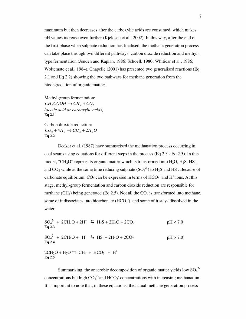
Woltemate et al., 1984). Chapelle (2001) has presented two generalised reactions (Eq
2.1 and Eq 2.2) showing the two pathways for methane generation from the
biodegradation of organic matter:
Methyl-group fermentation:
243 COCHCOOHCH +→ (acetic acid or carboxylic acids) Eq 2.1
Carbon dioxide reduction:
OHCHHCO 2422 24 +→+ Eq 2.2
Decker et al. (1987) have summarised the methanation process occurring in
coal seams using equations for different steps in the process (Eq 2.3 - Eq 2.5). In this
model, “CH2O” represents organic matter which is transformed into H2O, H2S, HS-,
and CO2 while at the same time reducing sulphate (SO42-) to H2S and HS-. Because of
carbonate equilibrium, CO2 can be expressed in terms of HCO3- and H+ ions. At this
stage, methyl-group fermentation and carbon dioxide reduction are responsible for
methane (CH4) being generated (Eq 2.5). Not all the CO2 is transformed into methane,
some of it dissociates into bicarbonate (HCO3-), and some of it stays dissolved in the
water.
SO4
2- + 2CH2O + 2H+ � H2S + 2H2O + 2CO2 pH < 7.0 Eq 2.3 SO4
2- + 2CH2O + H+ � HS- + 2H2O + 2CO2 pH > 7.0 Eq 2.4 2CH2O + H2O � CH4 + HCO3
- + H+ Eq 2.5
Summarising, the anaerobic decomposition of organic matter yields low SO42-
concentrations but high CO22-
and HCO3- concentrations with increasing methanation.
It is important to note that, in these equations, the actual methane generation process

8
takes place only after sulphate reduction has taken place. This is because sulphate
reduction is the dominant form of anaerobic respiration for non-methane-producing
bacteria. Also for this reason “biogenic methane does not accumulate in significant
amounts in the presence of high concentrations of dissolved sulphate” (Rice and
Claypool, 1981). Biogenic methane generated like this is normally referred to as early
stage. It estimated that most of the ancient biogenic gas accumulations took place in
this early stage (Rice, 1992; Rice and Claypool, 1981) over a period of tens of
thousands of years after burial (Claypool and Kaplan, 1974).
Gas and water production are directly related to the coal maturation process,
which is described by coal rank. Vitrinite is a type of organic material which is the
primary component of coal, and vitrinite reflectance is a parameter normally used to
establish the thermal maturity of coals (coal rank). Figure 2.1 presents the different
types of coal rank with matching vitrinite reflectance values. In terms of CSG
generation, thermogenic gas is formed when coals reach a certain level of thermal
maturity, which generally corresponds to high-volatile A bituminous coal (Scott,
2000). Low rank coals (peat, lignites, and sub-bituminous) have high porosities, high
water content, and low temperature biogenic methane (ALL-Consulting, 2003). As the
burial process continues, higher temperatures and pressures develop, making it
difficult for bacteria to survive (Nuccio, 2002). Thus biogenesis ceases and
thermogenesis begins. The thermogenic process is not just a temperature
transformation; it also involves chemical and physical transformations that result in
further coalification of the organic matter. In coalification, “coals become enriched
with carbon as large amounts of volatile organic matter rich in hydrogen and oxygen
are released” (Rice, 1993).

9
Coal Rank
Meta-anthracite
5.0
Anthracite
2.5
Semianthracite
1.91
Low-volatile bituminous
1.5
Medium-volatile bituminous
1.1
High-volatile A bituminous
High-volatile B bituminous
High-volatile C bituminous
0.49
Sub-bituminous A
Sub-bituminous B
Sub-bituminous C
0.38
Lignite
Figure 2.1. Coal Rank according to vitrinite reflectance (ASTM, 1983)
The released volatile organic matter is mainly methane, carbon dioxide, and
water. In addition, depending on the composition of the peat, some heavier
hydrocarbon gases and even oil may be released (Nuccio, 2002). With increasing
coalification (bituminous types), porosity decreases, water is expelled, and
temperature increases (ALL-Consulting, 2003). Therefore, the generation of
thermogenic methane occurs at high-volatile bituminous ranks and higher (Rice,
1993). This process can carry on until the coal is entirely transformed into anthracite;
as this takes place, less methane is generated , the coal porosity becomes even lower,
and most of the water is expelled (ALL-Consulting, 2003). Biogenic and thermogenic
processes can take place independently, in succession, or overlapping in time. For
example for sub-bituminous coals, biogenic methane generation rates decrease with
increasing temperatures and exhaustion of methanogenic bacteria. However, before all
methane-generating bacteria have died, some thermogenic methane is released from
Vitrinite reflectance( %
)

10
the coal material thus overlapping these two processes. If the organic-rich matter (i.e.
coal or organic matter undergoing coalification) is uplifted through tectonic forces,
then pressure and temperature are reduced thereby stopping the thermogenic
transformation and once again favouring biogenic generation.
Biogenic gas can be further generated in the Pleistocene or the Holocene
periods (tens of thousands to a few million years ago) long after the initial biogenic or
thermogenic processes (Rice, 1993). This can take place because coal seams can act
as regional aquifers with specific recharge zones and groundwater flowing through the
coal seams. Water can flow through coal seams because the coal material has a
network of fractures known as cleats, which give the coal adequate permeability for
water and natural gas flow. These cleats are formed in the coal maturation process
(coal dehydration, local and regional stresses, and changes in pressure) and they
control the directional permeability of coals (ALL-Consulting, 2003).
The new waters introduced into the system are loaded with microbes and may
have a high oxygen content. Figure 2.2 shows the recharge and water flow through a
generic coal aquifer. The hydraulic conductivity of such a coal aquifer system is not
necessarily low at shallow depths (10-6-10-4 m/s), but can decrease significantly at
depths greater than 100 m (Van Voast and Hedges, 1975). As these new oxygen
charged waters enter the recharge area and flow through the coal aquifer, the aerobic
decomposition process starts all over again. At this point, if there is a methane
generation process taking place then this process is interrupted because “methane-
producing micro organisms are strictly anaerobic and cannot tolerate even traces of
oxygen” (Rice and Claypool, 1981). However, additional oxidation of organic matter
will occur because organic matter (i.e. coal material undergoing further coalification)
is more degradable under aerobic conditions than under anaerobic environments
(Kjeldsen et al., 2002). This process results in the generation of a new food supply
and hydrogen ions, but finishes soon after the dissolved oxygen in the water is
depleted. This new food supply is basically anaerobically degradable organic matter
which can now get transformed into methane either by methyl-fermentation (Eq 2.1)
or by carbon dioxide reduction (Eq 2.2). Additionally, the new hydrogen ions (protons)
combine with bicarbonate generated in the early stage to form more carbon dioxide,
and more methane gas is generated through carbon dioxide reduction (Rice, 1993). It
is estimated that this process could take place in thousands of years depending on
specific conditions (Rice, 1993). In this way, CO2 reduction (Eq 2.2) is the main

11
process responsible for methane generation in coal seams acting as active aquifer
systems.
Figure 2.2. Water flow through coal aquifer system.
Coal seam gas storage and migration
The storage and migration of CSG is directly related to the flow of water in
coal seams, and to the physical and chemical structure of the coal. This structure is
often described as a block matrix containing micropores or internal coal surfaces
(Figure 2.3). This matrix is divided by a natural fracture or cleat system which is
generally saturated with water. The cleats form an orthogonal arrangement and can be
divided into face cleats and butt cleats. Face cleats (Figure 2.3) are dominant cleats
parallel to the maximum compressive stress and perpendicular to the fold axes.
Secondary cleats or butt cleats (Figure 2.3) are formed parallel to the fold axes and
terminate against face cleats (ALL-Consulting, 2003). In addition, the coal structure
may also include non-orthogonal cleats referred to as curvilinear cleats.

12
Figure 2.3. Cleat system and matrix blocks in coal (Gamson et al., 1996).
Therefore, gas storage and migration take place both at micro and macro levels.
At the micro level, the molecular structure of the coal acts as a virtual chemical cage
(Krevelen, 1961) capable of storing methane molecules. Therefore, gas is stored in the
coal’s micropores by means of absorption and adsorption. Because coal has a large
and complex internal surface area, large quantities of coal seam gas can be stored
within these surfaces by absorption (Rice, 1993). However, methane gas mainly
resides on the internal surfaces of coal (adsorption).

13
The combination of absorption and adsorption processes is often referred to as
sorption, and the reverse process is referred to as desorption. For the gas to remain
sorbed in the micro molecular cage, an external force (i.e. water pressure) must
constantly push the gas molecules into the coal micro structure, and the coal seam
must remain mostly confined. In coal seams, this is possible because groundwater
saturates and flows through the cleat system building up reservoir pressure, and thus
preventing the gas from escaping the coal microstructure (Rice, 1993). Impermeable
layers (clays, shales or mudstones) immediately on top or underneath the coal seam
can effectively act as confining layers for the coal seam aquifer. Thus, water is
prevented from escaping the coal seam and pressure increases as water flows through
the cleats.
Reservoir pressure at a given point (P) in the aquifer (Figure 2.5) can be
expressed as a function of hydraulic head, elevation, and water velocity (Eq 2.6).
Since water velocity (v) is extremely low for porous-media flow then the second term
of Eq 2.6 can almost always be neglected (Freeze and Cherry, 1979). For the aquifer
pressure to drop at point P, the hydraulic head value (h) or hp would have to drop
accordingly. When this happens (naturally or artificially), methane gas desorbs from
the internal surfaces of the coal. Methane gas then diffuses through the coal matrix
(micropores) until it reaches a cleat. At this point, the gas has reached the coal macro
structure (large pores and fractures or cleats) where it is stored and transported.
Diffusion from the coal matrix and gas flow through fractures can be modelled using
basic physical laws. The diffusion process is modelled according to Fick’s Law while
the free flow of gas and water through cleats is modelled using Darcy’s Law (Gamson
et al., 1996). Figure 2.4 shows the gas pathway after desorption and the procedure
normally used for modelling its flow. It has been estimated that coal can store
biogenic gas in this way up to “six or seven times the volume that can be stored in a
conventional natural gas reservoir of equal rock volume” (Nuccio, 2002). However, as
mentioned before, gas flow occurs only after fluid pressure acting on the internal coal
surface is reduced. This can take place naturally over time if there is tectonic
movement or uplifting of gas bearing coal seams, and water has “leaked” from the
coal aquifer or water flow is reduced. On the other hand, this can take place
artificially by human intrusion when water is pumped out at high rates from the coal
aquifer.

14
2)(
2vzhgPp
⋅−−⋅⋅= ρρ
Eq 2.6. (Freeze and Cherry, 1979)
where:
Pp = gage pressure at point p in the coal aquifer system
ρ = density of water g = acceleration of gravity h = hydraulic head z = elevation of point z with respect to a given datum v = groundwater velocity
Figure 2.4. Coal Seam Gas pathway and processes involved in its transport modelling. Adapted from Gamson et al (1993).
CSG mining procedure
Coal seam gas is typically mined by drilling a hole right into the coal seam
and then dewatering the coal aquifer to lower the hydraulic head, thus reducing the
aquifer pressure in the vicinity of the well (Figure 2.2 and Eq 2.6). Figure 2.5 shows a
typical production pod used in the Powder River Basin, located in the USA (ALL-
Consulting, 2003). The well is cased all the way down to the coal seam to effectively
isolate the coal seam and to prevent well collapse. In this schematic, a submersible
pump is used to dewater the coal seam, but other pumps can also be used (i.e. sucker
rod pumps). Because the well is cased all the way down to the coal seam, no energy is
wasted by lifting water from adjacent units. In principle, only CSG waters are being

15
pumped up to the surface, and no mixing with waters from other units can take place.
As the aquifer is dewatered, and the aquifer pressure drops, gas starts to diffuse from
the micropores. This gas can then flow from the coal matrix into the well cavity where
it then separates from the water. This gas flows through an outer pipe and is then fed
to a gas separator and compressor, while the CSG water flows through an inner pipe
into an impoundment or holding facility for its subsequent treatment and disposal.
Figure 2.5. Schematic of CSG production pod in the Powder River Basin (Wyoming State Engineers Office and Wyoming State Geological Survey, 2005).

16
Chemistry of waters associated with coal seam gas
Coal seam gas bearing aquifers have a specific water chemistry that relates to
geological, geochemical, physical, and biological processes. Underground, coal seams
are interbedded with other layers or units which can be mudstones, shales, or clays.
The geological and geochemical processes relate to the arrangement and
characteristics of adjoining units, while the physical processes relate to depth of burial,
potential tectonic uplifting, possible erosion (due to pumping for example), and
mixing of waters from other units. The biological factors affecting the chemistry of
these waters pose major implications particularly when the gas is of biogenic origin.
In essence, whether the processes involved are biogenic or thermogenic depends on
the depth of burial. The deeper the coal seam, the higher the temperatures and
pressures acting on it. On the one hand coal temperatures may be above the limit at
which methanogenic bacteria are able to survive, but on the other hand higher
temperatures and pressures increase the level of coalification in the seam.
Coalification is directly related to coal rank, which is a classification of coals mainly
relying on its moisture content, volatile matter, and calorific value. Low rank coals
comprise lignite and subbituminous coals having a low calorific value and a low
carbon content. High rank coals are bituminous or anthracitic coals which have a
higher calorific value and carbon content than lower rank coals.
In general, biogenic methane is associated with low rank coals, whereas
thermogenic methane is most likely linked to high rank coals. Most of the coal seam
gas (or coal bed methane) projects around the world are mining biogenic methane.
Normally, higher hydrocarbon gases (ethane and butane for example) and even oil are
produced with thermogenic gas. Therefore, thermogenic coal seam gas is generally
classified under a different category and referred to using a different name.
Nevertheless, most of the water quality properties associated with biogenic gas are
still applicable to waters associated with thermogenic gas.
In most biogenic CSG producing basins, coal seams act as regional aquifers
which are confined by nearly impermeable units (mudstones or shales). As recharge
water enters the coal seam, it flows very slowly and undergoes chemical and
biological transformations over the course of time. In addition, depending on each
particular scenario there may be infiltration from other units and some mixing may

17
occur. Nevertheless, tritium analyses of CSG water samples in the Powder River
Basin (Bartos et al., 2002) suggest that coal seam waters in coal aquifers are at least
submodern or pre 1950s. The different processes responsible for shaping the
chemistry of coal seam gas waters will be explained in the next paragraphs. Knowing
the conceptual chemical characterisation of these waters is important for the correct
interpretation of water quality samples taken from CSG bearing aquifers and for their
subsequent treatment and disposal.
Dissolution of Sodium Feldspars and Similar Minerals. As fresh
water seeps through recharge areas and flows through the coal aquifer, it encounters
different minerals along its path of flow. One of these minerals is sodium feldspar,
which can dissolve with recharge water (Figure 2.6) and increase Na+ concentrations
(Lee, 1981). When these minerals are of marine origin (albite and halite for example),
chloride concentrations can also increase with mineral dissolution.
Figure 2.6. Dissolution of sodium feldspars and ion exchange process in coal seam aquifers.

18
Bicarbonate concentrations. Coal seam gas waters always have a high
bicarbonate (HCO3-) content, which can be accounted for by two processes in the
aquifer. The first of these processes is the dissolution of carbonate by oxygenated
recharge waters (Freeze and Cherry, 1979). However, this process is not the primary
cause for the high HCO3-content in CSG aquifers. The second and primary process
accounting for high HCO3- content in CSG aquifers is methanation (Eq 2.5). As the
sulphate reduction process takes place, large amounts of HCO3- are produced and this
gives way to methanation. Other products of methanation include the generation of
aqueous carbon dioxide (CO2 (aq)) and a fairly alkaline pH. Therefore, the
concentrations of HCO3- in the aquifer will follow the speciation rules for a closed
aqueous carbonate system. The possible species available are CO32-, CO2 (aq), H2CO3,
and HCO3-. However, the fairly alkaline pH falls between 6.3 and 10.3 and, in this
range of values, HCO3- will be the dominant species according to carbonate chemistry
(Decker et al., 1987). Also, high pressure develops in the aquifer with increasing
depth, and this keeps CO32- in the HCO3
- form along with dissolved CO2 (aq). Figure
2.7 shows the evolution of recharge waters as these enter and flow through the coal
aquifer. When fresh water enters deeper parts of the coal aquifer, oxygen is depleted,
and anaerobic respiration takes place with increasing methanation and high
bicarbonate concentrations.

19
Figure 2.7. Evolution of bicarbonate concentration in coal seam gas waters.
Calcium and Magnesium depletion with ion exchange. Van Voast
(2003) has identified high HCO3- concentrations as the main cause for low Ca2+ and
Mg2+ concentrations in CSG waters. This is because the solubility of Ca2+ and Mg2+
decreases with high bicarbonate concentrations, which causes precipitation of calcite
(CaCO3) and dolomite (CaMg(CO3)2) in the aquifer. Another source of calcium and
magnesium depletion is given by the process of ion exchange. In coal aquifers,
groundwater may encounter clays or shales in adjoining units or in lenses or pockets
as it flows through the coal seam. Therefore, an ion exchange process takes place
between these minerals and the water itself. In this process, Ca2+ and Mg2+ are held
more tightly than Na+ in clays (especially in shales from marine origin with high
adsorbed Na+ ions). Therefore, the outcome of this exchange is a soft groundwater
(low Ca2+ and Mg2+) with an enhanced Na+ concentration. This process accounts for
the high Na+ and low Ca2+ and Mg2+ concentrations in CSG waters from the Powder
River Basin (Bartos et al., 2002), and it can be explained using the reactions in
equations Eq 2.7 and Eq 2.8 (Hem, 1985).
Na2X + Ca2+ �� CaX + 2 Na+ Eq 2.7����

20
Na2X + Mg2+ �� MgX + 2 Na+ Eq 2.8����
where Na+ = sodium ion Ca2+ = calcium ion Mg2+ = magnesium ion X = clay or shale
Studies by Hagmaier (1971), Lee (1981), and Hamilton (1970) suggest that
this process is more pronounced with increasing depth and away from sources of
recharge. Therefore as aquifer water flows into deeper parts of the basin, calcium and
magnesium concentrations gradually decrease due to ion exchanges with clays. The
same inversely holds true for sodium concentrations which would increase even
further with increasing aquifer depth (Figure 2.6).
Sulphate reduction. Sulphate (SO42-) increases when fresh recharge water
encounters and dissolves sulphate minerals (CaSO4, gypsum and anhydrite) along the
path of flow, or through the weathering and oxidation of pyrite and marcasite (FeS2)
(Bartos et al., 2002) and similar sulphide minerals. Sulphate is also present in sea
spray (Rosen et al., 2001) and, if coal seams are near the sea, it may deposit on
recharge areas and infiltrate into the aquifer. Organic matter (i.e. coal) first
decomposes aerobically with oxygenated recharge waters. However, as these waters
enter deeper parts of the aquifer, oxygen replenishment is no longer possible. The
process then turns to anaerobic decomposition as described by equations Eq 2.1- Eq
2.4. In the first phase of anaerobic decomposition (sulphate reduction), anaerobic
bacteria consume the available organic matter thus reducing sulphate concentrations.
A by product of the sulphate reduction process is the generation of dissolved
hydrogen sulphide (H2S); however, the presence of small traces of iron (Fe2+) will
cause hydrogen sulphide precipitation as black iron sulphides (Decker et al., 1987).
Once the majority of the sulphate is reduced, the anaerobic process can carry on to the
acidic and methanogenic phases (Rice and Claypool, 1981). In addition, depending on
the methanogenic species present in the aquifer, methane generation can take place
simultaneously with the sulphate reduction process (Oremland et al., 1982). However,
at high sulphate concentrations methane generation does not occur because, in this
situation, sulphate reduction becomes the dominant form of respiration.
With thermogenesis, sulphate reduction can take place with increasing
coalification, because coalification is basically a “metamorphism by pressure and heat

21
of burial” (Van Voast, 2003). Also, thermogenesis occurs in the absence of oxygen
because at the depths where this takes place, air or oxygenated water are not available.
Since there is no oxygen available, sulphide minerals are not able to oxidise and
generated sulphate ions.
Therefore, whether biogenic or thermogenic, CSG waters exhibit very low
sulphate concentrations (Figure 2.8). Van Voast (2003) has presented an upper limit
of 10 meq/l (~500 mg/l) for sulphate concentrations in co-produced water from
methane-producing wells in the US, which has useful exploration implications. The
10 meq/l upper limit was selected by Van Voast (2003) because this concentration
corresponds to the sulphate concentration of coal seam gas waters which are not
associated with the production of methane.
Figure 2.8. Sulphate reduction in CSG aquifers
Summarizing, the chemical signature of CSG waters can be described as high-
bicarbonate, high-sodium, low-calcium, low-magnesium, and low-sulphate. As
demonstrated by Van Voast (2003), different CSG producing basins in the United
States have approximately the same previously-stated chemical signature and almost
negligible sulphate concentrations (in many cases nil). This particular chemical

22
signature is useful for identifying CSG waters, which is useful during the exploration
phase. For example, if the abstracted water has a completely different signature than
the previously stipulated CSG water signature, and sulphate concentrations are higher
than 500 mg/l (Van Voast, 2003), then that well will most likely not produce methane
gas.
Differences with Acid Mine Drainage (AMD)
When certain minerals like pyrite and marcasite come in contact with water
and air (oxygen), oxidation reactions take place which result in the dissolution of iron,
sulphate, and a net increase in acidity. When this process occurs naturally, it is
referred to as Acid Rock Drainage, but when it is anthropogenic it is termed Acid
Mine Drainage. Equations Eq 2.9-Eq 2.12 are generally used to explain this process
(Stumm and Morgan, 1996). The oxidation of pyrite can be further increased with the
aid of iron-oxidising bacteria which can increase the oxidation rate of these minerals.
However, these bacteria operate only in Eq 2.10, at pH levels of below or around 3,
and the reaction is mostly abiotic.
+−+ ++→++ HSOFeOHOFeS s 2227 2
42
22)(2
Eq 2.9
OHFeHOFe 23
22
21
41 +→++ +++
Eq 2.10 ++ +→+ HOHFeOHFe s 3)(3 )(32
3
Eq 2.11 +−++ ++→++ HSOFeOHFeFeS s 16215814 2
42
23
)(2
Eq 2.12
Coal seams can have sulphur-bearing minerals such as iron sulphide, pyrite
(FeS2(s)), and marcasite, therefore they have acid producing potential. In this way,
water that has come in contact with coal under oxidising conditions, has generally a
low pH, metals dissolved in solution (iron, manganese, and aluminium), iron
hydroxide, and sulphate.
AMD waters in New Zealand have traditionally been associated with coal
mining operations. Therefore, people not familiar with CSG waters sometimes tend to
associate these waters to AMD. Coal seam gas waters are generated in an anoxic
environment therefore they do not oxidise sulphur-bearing minerals within the coal

23
seam. The biogenic processes of CSG formation produce water with a fairly neutral
pH, little or no dissolved metals, and very low sulphate concentrations. In this way
AMD and CSG are completely different processes yielding completely different
results. Table 2.1 shows two water quality samples from two NZ mines experiencing
AMD problems. These samples have a very acidic pH (below 3) and exhibit various
metals dissolved in solution (ferrous iron, manganese, aluminium, nickel, and zinc to
mention a few). Sulphate concentrations are also fairly high particularly in the Castle
Point Mine sample (829 mg/l). Other parameters of importance are total acidity and
specific conductance which are also high in both samples. These water samples do not
exhibit the geochemical signature for coal seam gas waters. In fact, they exhibit quite
the opposite chemistry: low pH, high calcium and magnesium in comparison to
sodium and chloride, high sulphate, and almost zero bicarbonate (Figure 2.9).
Figure 2.9. Schoeller diagram for NZ AMD samples.

24
Table 2.1. AMD water samples from two NZ mines.
Dissolved constituents Lower Sullivan Mine Discharge
Castle Point Mine
22/02/2001 02/04/2001 pH 2.86 2.53 Specific Conductance �S/cm� 9770 20100 Total Acidity (a) mg/l CaCO3 339 505 Sodium (Na+) mg/l 3.41 9.6 Potassium (K) mg/l 3.59 3.62 Calcium (Ca2+) mg/l 18.2 59.7 Magnesium (Mg2+) mg/l 8.74 33.1 Total Iron mg/l 83.7 15.4 Ferrous Iron (Fe2+) mg/l 47.1 14.5 Ferric Iron (Fe3+) mg/l 36.6 0.9 Manganese (Mn2+) mg/l 0.57 0.88 Barium (Ba2+) mg/l 0.01 0.01 Copper (Cu2+) ug/l 24.3 13.3 Nickel (Ni2+) ug/l 130 192 Zinc (Zn2+) ug/l 718 634 Aluminium (Al3+) ug/l 14300 58900 Arsenic (As3+) ug/l 3 < 0.001 Chromium (Cr2+) ug/l 3.3 25.5 Rubidium (Rb2+) ug/l 37.3 33.2 Lead (Pb) ug/l 1.2 1.9 Strontium (Sr2+) mg/l 0.09 0.36 Chloride (Cl-) mg/l 4.3 12.8 Boron (B) mg/l < 0.005 0.11 Bicarbonate (HCO3 -) (b) mg/l 0.07 0.04 Sulphate (SO4
2-) mg/l 56.9 829 Silica (SiO2) mg/l 34.4 NA Carbon dioxide (CO2 (aq)) (b) mg/l 256.7 297.24 Total Phosphorus (P) mg/l 2.33 < 0.004 Selenium (Se) mg/l < 0.001 < 0.001 Cobalt (Co) mg/l 0.0634 0.0629 Data supplied by CRL Energy. Sullivan Mine and Castle Point Mine are located in the West Coast, South Island (NZ). (a) Calculated from ferrous and ferric iron concentrations, aluminium, manganese, and pH. (b) Calculated from total acidity and carbonate equilibrium.
CSG water quality from US basins
In the 1980’s coal seam gas (or coal bed methane) began in the United States
with the government’s endorsement of tax credits for non-conventional energy
production. CSG production bloomed in the 1990’s, and by the end of 2000, CSG

25
production in the US totalled 3.831 trillion cubic metres (US Environmental
Protection Agency, 2004). The most important basins in the US include the Black
Warrior, San Juan, Raton, Piceance, Uinta, and the Powder River (Figure 2.10). This
last basin is important because it produces biogenic gas from low rank coals, which is
a similar scenario to the one in New Zealand. Nowadays, coal bed methane in the
United States plays a significant role in the energy market sector; in 2003 coal bed
methane accounted for about 8% of the US total methane production and proved
reserves for this resource increase at a rate of about 1% per year (Energy Information
Administration, 2004).
Figure 2.10. Major CSG producing basins in the United States. Adapted from Van Voast (2003).
Water quality from CSG producing basins has similar characteristics in terms
of geochemical signature (Na+ being the major ion), but can vary considerably in
terms of quantities produced and concentration of specific constituents. Table 2.2
summarises the water quality and quantity for six major CSG producing basins in the
United States. Water production across the different basins varies considerably. For
example, water production (per well) in the Black Warrior Basin is approximately 7.5
m3/day (Alabama State Oil and Gas Board (AOGB), 2003), whereas in the Powder
River Basin this figure reaches 63.6 m3/day (ALL-Consulting and Montana Board of
Oil and Gas Conservation, 2004). This is because CSG in the Black Warrior Basin is
of thermogenic origin, therefore coal porosity in this basin is low in comparison to
coal porosity from biogenic origin reserves such as the one in the Powder River Basin.

26
Low rank coal and lignites (biogenic methane) have high porosities whereas high rank
(thermogenic origin) have low porosity and lower water content (ALL-Consulting,
2003). Therefore, a larger quantity of CSG waters is expected from biogenic methane
reservoirs which needs to be managed accordingly. This can be observed by analysing
the differences in the Water/Gas ratio presented in Table 2.2. Here, the Powder River
Basin presents an impressive 17.33 m3/TCM ratio (ALL-Consulting and Montana
Board of Oil and Gas Conservation, 2004), which is a good indicator of the number of
issues that arise from water disposal operations associated with CSG extraction. This
is exacerbated when considering the salinity of these waters; in CSG waters the major
ion present in solution is sodium, which can have detrimental effects to soils and
surface waters if not adequately disposed. Another chemical property presenting
significant variations is TDS. In general, this value increases with coal rank, depth,
and distance from main recharge areas. In sites like the Powder River Basin this value
does not seem very high; however, due to the large quantities of water involved, this
parameter can pose serious risks when managing CSG waters. These variations
suggest carrying out an in-depth study of the chemical nature and signature of CSG
waters.
The study of CSG waters involves the determination of important chemical
properties like pH, TDS, and the concentration of major and minor ions. Once this
information is collected, it needs to be put in context or compared against the
composition of surface waters and other CSG waters. For example, Piper diagrams
(Freeze and Cherry, 1979) are used for grouping and presenting samples according to
their major ion composition, and Schoeller diagrams (Freeze and Cherry, 1979) are
used for comparing samples in a quantitavely manner. The chemical signature for
these six major producing basins has been presented by Van Voast (2003) using the
Schoeller diagram representation (Figure 2.11). Figure 2.11 shows the geochemical
signature for CSG waters (defined in the previous section) which corresponds to the
outcome of the conceptual model for the genesis of coal seam gas waters. In this
figure, it is possible to compare the proportion of ions for individual water samples
within (and between) basins. In this way, calcium and magnesium concentrations are
low in comparison to sodium and bicarbonate ones. In addition, sulphate
concentrations are always low as a result of the sulphate reduction process prior to
methogenesis; sulphate concentrations are always below the previously defined

Table 2.2. CSG water quantity and quality from selected US basins.
Basin State N° Wells�
Average Water Production
Gas Water/Gas Water type (c) pH(c) TDS(c) TDS
m3/day /well TCM/day/well m3/TCM mg/l mg/TCM/well
Black Warrior AL 3423 (a) 7.5 (a) 2.6 (a) 2.86 Na-Cl-HCO3 5.4-9.9 160-31,000 134-25901 Powder River WY,
MT 13880 (b) 32.9 (b) 1.9 (b) 17.33 Na-HCO3 6.8-8.0 270-3,010 337-3758
Raton CO 694 (c) 42.3 (c) 8.5 (c) 4.98 Na-HCO3 6.0-7.9 (e) 86-2,582 (e) 617-18527 San Juan CO,
NM 3089 (c) 4.0 (c) 22.7 (c) 0.18 Na-HCO3-Cl 5.2-9.2 410-171,000 24-9964
Uinta UT 558 (c) 34.2 (c) 17.7 (c) 1.93 Na-HCO3-Cl 7.0-8.2 6,350-42,700 21963-147690 Sources: (a) (Alabama State Oil and Gas Board (AOGB), 2003). (b) (Nelson, 2005)
(c) (PTTC, 2000); (GRI (Gas Research Institute), 2000); (US Environmental Protection Agency and Advanced Resources International, 2002); CO, NM, WY, MT Oil and Gas Commissions; (Williams. B, 2001). These sources are quoted in ALL-Consulting and Montana Board of Oil and Gas Conservation (2004). (d) (Rice and Bartos, 2001). (e) (The Seacreast Group, 2003) TCM = Thousand cubic metres of gas

28
limit (10meq/l) for methane production in wells drilled directly into coal seams (Van
Voast, 2003). Figure 2.11 also shows varying degrees of chloride concentrations
amongst the different basins. This is even more noticeable in basins presenting strong
marine associations (Black Warrior, San Juan, Piceance, and Uinta).
Differences within basins can be attributed to well depth and their distance to
recharge areas, as well as water age. As water flows through a coal seam gas basin, it
dissolves and mixes with minerals along its path of flow. This process has been
explained in detail throughout this chapter, but it is important to underscore that the
closer a well is to the recharge area, the less mineralised the resulting water will be.
The same holds inversely true for deeper parts of the basin: the closer a well is to the
deepest part of the basin, the more mineralised the resulting CSG water will be. In the
Powder River basin, for instance, CSG water produced on the basin margins has a low
TDS suitable for human consumption (<500 mg/l); however, in inner parts of the
basin this water has TDS values as high as 3010mg/l (Table 2.2) rendering it
unsuitable for most beneficial applications.

29
Figure 2.11. Schoeller diagrams for CSG producing basins in the United States (Van Voast, 2003).

30
Figure 2.12. Piper diagram for six major basins in the United States. Data taken from Van Voast (2003).
The data presented in Figure 2.11 can also be plotted in a Piper diagram
(Figure 2.12) to visually group all of the samples for the selected basins and to
identify major trends. In this way, all of the samples have sodium as a major ion,
followed by bicarbonate or chloride. Samples for Uinta (Buzzard Bench), Piceance
(shallow), and Raton (centre) basins are of the Na+-HCO3--Cl- type, while samples for
Uinta (Drunkards Wash), Piceance (deep), and Black Warrior (Oak Grove Field)
basins are of the Na+-Cl--HCO-3 type. In the cases of Uinta and Piceance, the second
major ion (Cl- or HCO3-) can vary depending on the location of wells within the basin
from which samples are extracted. In general, Cl- concentrations near recharge areas
are lower than in deeper parts of the basin (Van Voast, 2003), and this could explain
why Cl- is the second major ion in Piceance (deep) but the third major one in shallow
parts of this basin (Piceance, shallow in Figure 2.11). The water quality for San Juan,
Powder River, and Raton (north) basins is of the Na+- HCO3- type. These waters have
little or no chloride, which is believed to be due to the proximity to recharge areas
(San Juan and Raton, North) or to their non marine nature in the case of the PRB (Van
Voast, 2003). In all of these cases, however, the major cation is sodium.

31
CSG water quality from potential New Zealand basins
New Zealand has been following the developments of coalbed methane (coal
seam gas) in the US with keen interest. The first ones to explore this technology in
New Zealand were R C Macdonald and Partners Ltd who established Southgas Ltd in
1984. Southgas explored the CSG potential of the Ohai Coalfields. They obtained
good gas results, however their project was incompatible with the coal mining project
established at the site, so Southgas had to abandon this operation (Johnson, 2004). In
the mid 1990’s they changed their name to Westgas Ltd, and they devoted themselves
to the Greymouth Coalfield. Here, Westgas has tapped into significant amounts of gas
from sandstone-coal reservoirs, but exploration and production issues still need to be
resolved before commercialisation (Cave, 2002).
Up to 1990 there was a generalised belief that CSG could only be minable if it
was a consequence of the thermogenic processes in bituminous (high-rank) coals
(Johnson, 2004). However, in the 1990’s developments in the Powder River Basin
(US) proved that commercially quantities of coal seam gas could be recovered from
low-rank coals (Johnson, 2004). New Zealand coals present some of the same
characteristics as those found in the Powder River Basin (Moore, 2002). Therefore,
New Zealand coals hold significant potential for CSG development and extraction.
Many companies seized this opportunity, and since the 1990’s have obtained different
exploration licences. Kenham Holdings, for example, has acquired CSG exploration
licenses covering the lignite deposits of Central Otago and Eastern Southland, and a
licence to explore the sub-bituminous coal seams of the Maramarua Coalfield. In
addition, Kenham has an exploration licence for the bituminous resource in the Buller
and Reefton coalfields, located in the New Zealand South Island. Other companies
that have joined the CSG play include Resource Development Technologies (Waikato
coal region), Solid Energy (Taranaki and the South Island West Coast), and Bridge
Petroleum (Southern Waikato Coal Region and King Country).

32
Methods
Since 2000 Kenham Holdings, with the aid of CRL Energy Ltd and L&M
Mining Ltd, has been exploring and developing the CSG resource in New Zealand. As
part of their work these companies determine which coal fields hold better potential
for CSG extraction, characterise the gas held in those coal seams, and produce
estimates on the quantity of gas that could eventually be extracted. The licenses under
exploration are for lignites and sub-bituminous coals, therefore these would only
involve biogenic methane. The exceptions are Buller and Reefton which would hold
bituminous coal reserves. The CSG water disposal issue was acknowledged by these
companies for the successful development of CSG projects in New Zealand.
In 2003, CRL Energy Ltd collected water samples from their drilling
operations. These samples were often collected by field operators only when the
opportunity presented itself – that is, when artesian conditions were encountered or
when water was air-lifted to clear the boreholes in order to carry out basic falling head
tests. In a few instances, samples were collected personally, but in the majority of
these cases, samples were collected without following any sampling protocols (i.e. no
prior purging); samples were analysed anyway to prove that a proper sampling
programme was indeed necessary to produce high quality data.
It should be noted that the methods used for much of this research are non-
ideal; however, they were necessary given the business and political pressures on the
partners in the research, CRL Energy Ltd and L&M Mining Ltd. This matter and the
methods used by on-site personnel for collecting these samples are discussed in some
detail in section A.3 (Appendix 3). Figure 2.13 shows the exploration sites from
which water samples were collected and analysed. In some cases samples were sent to
certified laboratories for full analysis, but in other cases samples were analysed just
for major ions and basic chemical properties at the Environmental Engineering
Laboratory (EEL, University of Canterbury).
Hill Laboratories and the CRL Energy laboratory are certified labs in New
Zealand. These labs operate following guidelines from the APHA (American Public
Health Association. et al., 1999) with very low detection limits. Therefore, when
possible, the same standard was used at the EEL (University of Canterbury). When

33
this was not possible, HACH methods or analytical procedures were used to
complement the sample analysis.
In sum, because of business and political decisions the choice of sample
collection and analyses were in many cases non-ideal methods. To remediate the
situation and validate the data collected, a higher analytical treatment and
interpretation of the data was later carried out throughout this work (i.e. Chapters 3-5
and Appendix B.2). Sample analyses (TDS, alkalinity, hardness, and calcium) at the
EEL (University of Canterbury) were carried out using the Standard Methods from
the APHA (American Public Health Association. et al., 1999). In addition, sulphate
and chloride were analysed using HACH methods (Hach Company., 2003), and pH
and Specific Conductance were measured using calibrated metres. Once these
analyses were carried out, it was straight forward to compute the bicarbonate content
(from carbonate equilibrium) and magnesium concentrations (from hardness and
calcium concentrations). It was then possible to estimate sodium concentrations by
assuming zero electro neutrality in the water samples. A summary of these methods is
presented in Appendix A, section A.1.

34
Figure 2.13. Kenham Holdings sites from which water samples have been collected.

35
CSG exploration in New Zealand
Water samples from the locations in Figure 2.13 indicate that the sampled
water is not CSG water. This is mainly because the boreholes at those locations were
not cased down to coal, and the techniques used for sampling the boreholes were not
adequate for sampling CSG waters (i.e. not enough purging). Notwithstanding,
sample results and analyses for Ashers-Waituna, Reefton, Kaitangata, and Hawkdun
are presented in Appendix A (A.2). These results do not follow the geochemical
signature of CSG waters, and therefore are not what could be expected from real CSG
dewatering operations. In 2004-2005, however, good CSG water samples were
obtained for a location in Maramarua. Consequently, results from Maramarua
exploration and sampling are presented in the following paragraphs.
Maramarua. The Maramarua coalfield (Figure 2.14) has good potential for
CSG development because its Kupakupa Seam contains substantial amounts of sub-
bituminous coal (Pope and Trumm, 2004). The 20m thickness of the Kupakupa Seam
would facilitate CSG production because wells targeting that seam would cover a
large vertical surface area within the seam itself. Coal from this field generally has
low ash and sulphur contents and is of the sub-bituminous C-B type. The Eocene
Kupakupa Seam has impermeable claystone cap rocks which prevents water (and gas)
from escaping the seam; this seam has been identified as an aquifer with sufficient
hydrostatic head capable of preventing natural CSG desorption (Pope and Trumm,
2004).
In August 2003, borehole C1 was drilled in the Clifton sector of the
Maramarua Coalfield (Figure 2.14). The drill penetrated through different layers of
clay, and mudstone before reaching an 11.55 m layer of coal (Kupakupa Seam). It
then went through two thin layers of mudstone and coal and then stopped at a depth of
207m (Table 2.3). This well had sub artesian pressure, and the well had to be sampled
using a pump capable of purging the well and collecting a sufficient volume of water
for analysis. This was carried out by a subcontractor (D. J. Phelps & Co Ltd) who
used a Grundfos submersible pump (MP1) to purge the well until pH, temperature,
and conductivity became stable. This pump was small enough (φ=50mm) to fit down
the borehole (≈100mm), but was quite effective in extracting at least 380 litres of

36
water before collecting the actual sample. The sample was collected in this fashion on
the 18/9/2003 and subsequently analysed at Hill Laboratories. The results of this
analysis are presented in Table 2.4. As with the Hawkdun samples, the borehole was
not cased all the way down to coal level, therefore this sample does not exclusively
represent coal seam waters. In this way, water from other units (i.e. mudstones,
sandstones and siltstones) had the possibility of entering the hole and mixing with
coal seam waters. The 18/9/2003 sample has the chemical signature of CSG waters:
high pH, low calcium and magnesium concentrations, and high sodium and
bicarbonate. The sulphate concentration for this sample is reasonably low (27.6 mg/l)
and below the concentration for the limit of methane production (500 mg/l) in wells
presented by Van Voast (2003). The major ions for this sample are sodium and
bicarbonate, therefore this water is classified as of the Na-HCO3- type. It is also worth
noting the relatively high chloride and iron concentrations (49.3 mg/l and 55.9 mg/l),
the high DOC (130 mg/l), and the high value for total hydrocarbons (mostly C10-
C14).
Some key measurements were taken on site while carrying out the sampling.
For example, the on site measurement for pH is 7.5 and the specific conductance 1200
µS/cm. These values differ significantly to the ones taken by Hill laboratories which
suggest the possibility of a mistake in the laboratory data. This was further
corroborated when the TDS value was calculated manually from the data presented in
Table 2.4 and using Eq 2.13. In this way, the calculated TDS value is 696 mg/l which
is 65% of the value reported by Hill Laboratories (1160 mg/l). TDS and Specific
Conductance are related through common approximations, and can be expressed in
terms of each other using Eq 2.14 and Eq 2.15 (0.54 < A < 0.96). The TDS value
reported by Hill Laboratories exceeds by far the reported value for Specific
Conductance (718 µS/cm) reported along with TDS, and thus contradicts Eq 2.15.
Furthermore, the Specific Conductance calculated using Eq 2.14 and the data in Table
2.4 (980 µS/cm) is higher than the one reported by Hill Laboratories (718 µS/cm) and
closer to the value measured on site (1200 µS/cm). A conservative approach for these
two values would be to adopt the on site measurement for Specific Conductance
(1200 µS/cm) and the calculated TDS value (696 mg/l).

37
TDS (mg/l) = Σ ions (mg/l) + SiO2 (mg/l) – [HCO3- (mg/l)·�0.5082]�
Eq 2.13. (Hounslow, 1995) Specific Conductance (µS/cm) = SUM of cations (meq/l) *100 Eq 2.14 (Hounslow, 1995) TDS (mg/l) = A · Specific Conductance (µS/cm)�Eq 2.15 The value of A ranges from 0.54 to 0.96, but usually assumes values between 0.55 and
0.76 depending on the water being analysed (Hounslow, 1995). For the particular case
of the Maramarua CSG samples, A ranged from 0.51 to 0.62

38
Figure 2.14. Location of borehole C1
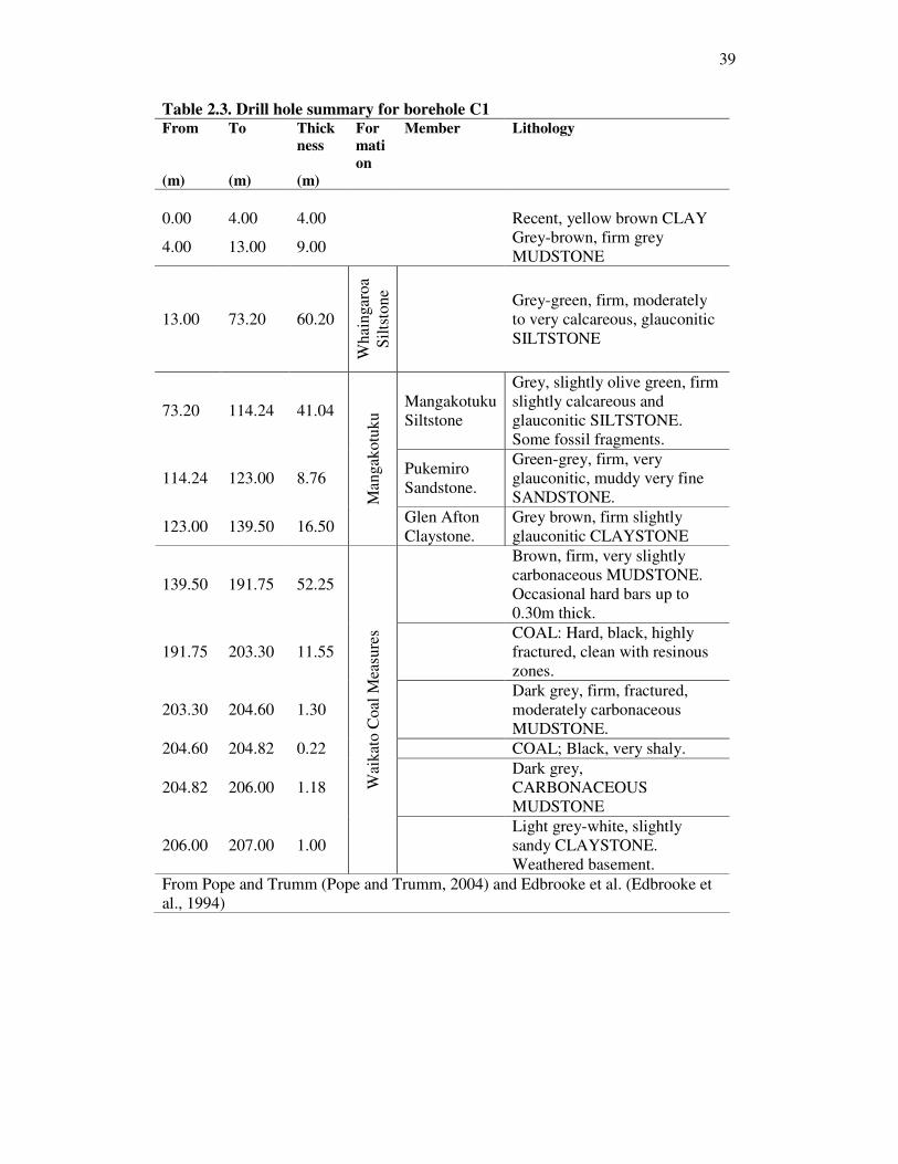
39
Table 2.3. Drill hole summary for borehole C1 From To Thick
ness Formation
Member Lithology
(m) (m) (m) 0.00 4.00 4.00 Recent, yellow brown CLAY
4.00 13.00 9.00 Grey-brown, firm grey MUDSTONE
13.00 73.20 60.20
Wha
inga
roa
Silts
tone
Grey-green, firm, moderately to very calcareous, glauconitic SILTSTONE
73.20 114.24 41.04 Mangakotuku Siltstone
Grey, slightly olive green, firm slightly calcareous and glauconitic SILTSTONE. Some fossil fragments.
114.24 123.00 8.76 Pukemiro Sandstone.
Green-grey, firm, very glauconitic, muddy very fine SANDSTONE.
123.00 139.50 16.50
Man
gako
tuku
Glen Afton Claystone.
Grey brown, firm slightly glauconitic CLAYSTONE
139.50 191.75 52.25
Brown, firm, very slightly carbonaceous MUDSTONE. Occasional hard bars up to 0.30m thick.
191.75 203.30 11.55 COAL: Hard, black, highly fractured, clean with resinous zones.
203.30 204.60 1.30 Dark grey, firm, fractured, moderately carbonaceous MUDSTONE.
204.60 204.82 0.22 COAL; Black, very shaly.
204.82 206.00 1.18 Dark grey, CARBONACEOUS MUDSTONE
206.00 207.00 1.00
Wai
kato
Coa
l Mea
sure
s
Light grey-white, slightly sandy CLAYSTONE. Weathered basement.
From Pope and Trumm (Pope and Trumm, 2004) and Edbrooke et al. (Edbrooke et al., 1994)

40
Table 2.4. Maramarua C1 samples Sample date 18/09/2003 (1), (3) 19/08/2004 (2), (4) pH pH units 8.5 7.8 Specific Conductance (T=25ºC)
µS/cm� 1200 (6) 1310
TDS mg/l 696 (7) 782 Hardness mg/l as CaCO3 76.7 (7) 18 Alkalinity mg/l as CaCO3 340 360 Bicarbonate (HCO3 -) mg/l 402 435 (5) Carbonate (CO3
2-) mg/l 8.8 (5) <2 Carbon dioxide (CO2 (aq)) mg/l 4.2 (5) 25 Calcium (Ca2+) mg/l 20 6 (3) Magnesium (Mg2+) mg/l 6.5 0.9 (3) Sodium (Na+) mg/l 184 334 (3) Potassium (K) mg/l 9.5 3 (3) Chloride (Cl-) mg/l 49.3 146 Sulphate (SO4
2-) mg/l 27.6 0.7 Fluoride (F) mg/l 0.32 0.79 (3) Boron (B) mg/l 1.95 2.5 (3) Silica (SiO2) mg/l 3.5 10.7 (3) DOC mg/l 130 11 (3) Total Iron (Fe) mg/l 55.9 0.4 (3) Manganese (Mn) mg/l 0.242 <0.01 (3) Arsenic (As) mg/l <0.01 <0.02 (3) Barium (Ba2+) mg/l 0.154 0.024 (3) Chromium (Cr2+) mg/l 0.031 <0.01 (3) Mercury (Hg) mg/l 0.0009 <0.002 (3) Selenium (Se) mg/l <0.01 <0.02 (3) Zinc (Zn2+) mg/l 0.17 1.28 (3) Hydrocarbons C7-C9 mg/l <0.3 <0.03 (3) Hydrocarbons C10-C14 mg/l 117 <0.05 (3) Hydrocarbons C15-C36 mg/l 4 <0.1 (3) Hydrocarbons Total mg/l 121 <0.2 (3) (1) This sample was collected from the borehole prior to casing installation (to isolate the coal seam from other units). (2) This sample was collected after borehole C-1 had been re-drilled and cased down to coal thus effectively isolating the coal seam. (3) Sample was analysed by Hill Laboratories, Hamilton, and NZ. (4) Sample was analysed by the CRL Energy Ltd Laboratory, Wellington, NZ. (5) Calculated from carbonate equilibrium. (6) On site measurement (7) Calculated from measured ion concentrations

41
Exploration hole Maramarua C-1 was redrilled in June 2004 for the purpose of
conducting a gas flow test. The well was completed with steel casing (100 mm) all the
way down to the coal seam, effectively isolating it from nearby units, and thus
preventing the mixing of coal seam waters with waters alien to the coal formation.
This enabled the efficient pumping of water from the coal seam thereby reducing
hydrostatic pressure and promoting desorption and gas flow. Once the gas flow test
started, it was possible to collect samples for analysis.
On 19/8/2004 one sample was collected and sent to CRL Energy Ltd in
Wellington where a detailed analysis was carried out. Results for this analysis are
presented in Table 2.4 alongside the results from the sample taken from the uncased
borehole on the 18/09/2003. The 19/8/2004 sample fits more closely the geochemical
signature for coal seam gas waters than the 18/09/2003 sample. For example, calcium
and magnesium concentrations are even lower in the 2004 sample than in the 2003
sample (70% and 86% less respectively), and bicarbonate and sodium concentrations
are higher (8.2% and 81.5% higher respectively). In this case, chloride concentrations
are higher than before, reaching a value of 146 mg/l (196% higher than the original
value). Of significance is the fact that sodium levels have increased by almost 82%.
Also, DOC values have decreased to 11 mg/l while iron levels have decreased
significantly (0.4 mg/l). In general, most trace elements decreased in concentration
except for zinc which increased moderately in 2004 (from 0.17 to 1.28 mg/l).
The Total Hydrocarbons for this sample are almost non-detectable (<0.2 mg/l)
and the sulphate concentration is very low (0.7 mg/l which constitutes a 97.4%
decrease in the 2003 value). The most likely reason behind these differences lies in
the fact that for the second round of sampling (August 2004) the well was cased down
to coal. Thus, when the well was sampled, one would expect that only water from the
coal seam would enter the well, whereas in the previous sampling round (September
2003) one would expect that the sampled water was a mixture of coal seam water and
water from other units (sandstones, siltstones, and mudstones). The 2004 values for
Specific Conductance and TDS compare better to the on-site measurements taken
during sampling in 2003 than to the subsequent lab results. This confirms the
hypothesis that the 2003 laboratory results were erroneous (most likely a typographic
error in writing down these values or swapping them by mistake). A noticeable
difference is the high chloride composition in the August 2004 sample which
classifies these CSG waters as Na-HCO3--Cl. This is possible because the 2004

42
sample is not expected to contain water from units other than coal and thus, the high
chloride content in the pure CSG water would not be expected to have been diluted
out as in the previous case.
Differences between the 18/09/2003 sample and the 19/8/2004 sample can be
observed graphically by the use of Piper (Figure 2.15) and Schoeller (Figure 2.16)
diagrams. The 18/9/2003 sample has a different ion composition than the 19/8/2004
sample. This can be observed graphically by inspecting the Piper diagram on Figure
2.15; on this diagram both samples plot at a different location.
Figure 2.15. Piper diagram for Maramarua C-1 samples
The Schoeller diagram (Figure 2.16) shows that calcium, magnesium, and
sulphate concentrations are higher in the 2003 sample than in the one taken in 2004.
Sodium and Chloride, however, tend to be lower. In both of these samples sulphate
levels are below the limit of 500 mg/l (≈10meq/l) for methane producing wells in the
United States (Van Voast, 2003). This value is lower in the 2004 sample than in the
2003 sample, which is promising in terms of methane production. Because of the steel
casing installation, one would expect that the Schoeller diagram for the 2004 sample
presented in Figure 2.16 represents the true geochemical signature for CSG waters in
Maramarua. At this stage it is interesting to note that desorption results from coal
canisters taken from this borehole indicate that this coal seam holds significant
amounts of methane (Pope and Trumm, 2004). Since the coal type is sub-bituminous,
it is not likely for this methane to have been generated by thermogenesis; therefore

43
this methane must have been generated by biogenic processes, which in turn produce
CSG water with the previously defined geochemical signature.
�
Figure 2.16. Schoeller diagram for Maramarua C-1 samples.
Very low tritium concentrations (-0.003 ± 0.016 TU) in samples collected on
the 20th and 21st of October, 2004, suggest there is no recent recharge in the
Maramarua coal aquifer. A qualitative interpretation of this value (<0.8 TU) classifies
this water as sub-modern or pre-1952 (Clark and Fritz, 1997). Since tritium
concentrations are basically nil, then the aquifer is either confined or so deep that
recharge takes a long time. Log bore data (Table 2.3) taken while the well was being
drilled suggests the aquifer is confined by a 16.5 m claystone cap (Pope and Trumm,
2004). Therefore, if no dispersion is assumed within the aquifer, then it is possible to
apply a piston flow model (PFM) for a quantitative estimate of residence time. A
PFM is a model that assumes little or no dispersion; it has been compared to a train
moving people on a single path as opposed to people travelling in cars on a highway
(Clark and Fritz, 1997). Consequently, the PFM assumes tritium concentrations
change only due to isotopic decay (Maloszewski and Zuber, 1982). According to this,
water from the Maramarua C-1 well would be at least older than 86 years.

44
A high transit time in the coal aquifer means CSG waters are subjected to
geochemical processes as they flow through the seam. This leads to a more
quantitative interpretation of the Maramarua CSG water samples using the source-
rock deduction method described by (Hounslow, 1995). In this method, different
ratios of chemical constituents give insight into the origin of the water being analysed.
The attention values used in this method are derived from a mass balance approach
using collections of water quality data (Hounslow, 1995), therefore this method can
give a good estimate on the origins of a particular water. The calculated ratios for the
19/8/2004 sample, their attention values, and conclusions are presented in Table 2.5.
The first ratio, which has to do with the proportion of sodium and chloride ions in
halite (NaCl), indicates there is extra sodium (not accounted by halite dissolution)
which could have resulted from the dissolution of albite (sodium feldspars) or an ion
exchange process. However, the second ratio which tests for nonhalite sodium
indicates that the extra sodium is not likely to originate from plagioclase (albite)
weathering. Therefore, the main process responsible for enhancing sodium
concentrations would have to be ion exchange. This is confirmed by comparing silica
concentrations with nonhalite sodium using the third ratio on Table 2.5. Because silica
concentrations are low in comparison to nonhalite sodium, then the majority of the
sodium is likely to have taken place through a cation exchange process.
The fourth ratio indicates that there is more calcium than sulphate in the water
and this would indicate carbonate weathering. The same conclusion is reached when
analysing the ratio of bicarbonate and silica. A high TDS value and the magnesium
concentrations relative to calcium (sixth and seventh ratios) point towards carbonate,
limestone and dolomite weathering. However, high bicarbonate concentrations can
also result from methane generation processes, which also account for the low
sulphate concentrations in the CSG water. Therefore, it is possible that some
carbonate weathering did occur, but bicarbonate concentrations were enhanced and
sulphate concentrations were reduced through the methanation process. According to
the last ratio in Table 2.5, the low chloride concentrations in the water sample are due
to rock weathering. This is possible if there is some halite dissolution processes taking
place. Lastly, the calculated Langelier Index for this sample is -0.48 which indicates
that the sample is undersaturated with respect to calcite. However, this value can
change once the sample is exposed to local atmospheric conditions. Sparging
experiments conducted at the EEL have yielded positive Langelier Indexes for the

45
same type of water. This means that, once these CSG waters reach equilibrium with
the atmosphere, they become oversaturated with calcite so they precipitate calcium
carbonate.
Table 2.5. Rock-source deduction based on elemental rations (Hounslow, 1995). Parameter value attention
value conclusion
[Na+] / [Na++ Cl-] 0.8 >0.5 Sodium source other than halite: albite or ion exchange
[Na++K+-Cl-] / [Na++K+-Cl-+Ca2+] 0.001 <0.2 Plagioclase weathering is unlikely
[SiO2] / [Na+ + K+ - Cl-] 0.02 <1 Cation exchange [Ca2+] / [Ca2+ + SO4
2-] 0.95 > 0.5 Calcium source other than gypsum: carbonates or silicates
[HCO3-] / [SiO2] 40 > 10 Carbonate weathering*
[Mg2+] / [Ca2+ + Mg2+] 0.2 <0.5 and * Limestone-dolomite weathering
TDS (mg/l) 782 >500 Carbonate weathering or brine or seawater
[Cl-] / Sum [Anions] 0.3 <0.8 Rock weathering Langelier Index -0.48 <0 Undersaturated with respect
to calcite Notes: Ratios were calculated with concentrations in meq/l. This source-rock deduction was carried out on the sample collected on the 19/8/2004. This sample was sent to Hill Laboratories (certified lab) for a full ion concentration analysis yielding very good results (electroneutrality = 4%).
Summarising, the majority of the sodium would originate from ion exchange
processes in the aquifer. Some halite dissolution would be responsible for some
sodium and the majority of the chloride. High bicarbonate concentrations would be
due to carbonate weathering and biogenic (methanogenic) processes which are also
responsible for low sulphate concentrations. Carbonate and dolomite weathering
would also be responsible for calcium and magnesium concentrations. However,
because of the high bicarbonate content, these cations would rapidly precipitate out of
solution in the aquifer. In addition, the same ion exchange process responsible for
sodium enhancement aids in the depletion of calcium and magnesium concentrations.

46
Discussion
Coal seam gas exploration in New Zealand has enabled the possibility of a
new energy source with promising economic prospects. However, this technology will
co-produce CSG water which, if not dealt with properly, can cause environmental
problems due to its quality and quantity.
Based on the limited data able to be presented here, CSG waters in New
Zealand do not differ much to CBM waters in the United States. This has been
determined by analysing Maramarua water samples, which have been the best
samples so far in terms of obtaining true CSG waters. Other samples, like the first
Maramarua sample and samples from other locations, have helped to assess the
correct sampling procedure which would go hand in hand with CSG mining
operations. For example, in normal CSG mining operations each well would be
continuously pumped to lower the coal aquifer pressure and to desorb and mine the
coal seam gas. Constant pumping would flush the well of drilling fluids and stagnant
water, and would produce large amounts of water referred to as CSG waters. Samples
taken from exploration boreholes without adequate pumping (Reefton, Kaitangata,
and Ashers Waituna; see Appendix A) are non indicative of CSG waters. These holes
could have contained a large proportion of stagnant water and drilling fluids. Another
issue to consider is casing. Casing in production wells is important because it
effectively isolates the coal seam from other units above or below it. This ensures that
only the coal seam is effectively being dewatered while increasing efficiency and
decreasing the amount of co-produced water. This is particularly important if the
adjacent formations have a high concentration of ions that could increase the chemical
loading of CSG waters. More so, having a lower amount of better-quality water to
dispose of is always better than the alternative. Consequently, the Maramarua C-1
well was cased in 2004 to carry out a gas flow test, which involved the pumping of
large amounts of water. Therefore, samples from this well truly reflect the nature of
coal aquifer waters (CSG waters).
The Maramarua CSG samples have a geochemical signature that is consistent
with the signature for CSG waters defined by Van Voast (2003). This signature
validates the model for the genesis and evolution of CSG waters flowing through the
coal aquifer. As follows, Maramarua CSG waters have low calcium and magnesium
concentrations in comparison to sodium and bicarbonate. Chloride concentrations are

47
also high, and constitutes the third major ion dissolved in these waters. Sulphate
levels are very low (<2mg/l); lower than the 500 mg/l limit set by Van Voast (2003)
for methane producing wells in the US.
Chemical analysis (rock source deduction) of Maramarua CSG water samples
provides insight into the origins and processes involved in shaping this particular
water quality. This method is a simple approach but is a good way of verifying an
actual sample’s origins especially if specific biogeological processes are suspected to
have taken part in its formation. In the case of Maramarua, these processes are a
combination of weathering of rocks (carbonates, dolomite, and halite), cation
exchange, and biogenic processes. Nil tritium concentrations suggest aquifer recharge
is taking place at a very slow rate, which would allow enough time for the CSG water
generation processes to take place.
Figure 2.17. Maramarua CSG water compared against CBM samples from US basins. Sources: CRL Energy and Van Voast (2003). Sulphate concentrations for US sites may be lower than 0.1 meq/l.

48
Figure 2.18. Piper diagram for NZ CSG water samples compared against US CBM and NZ AMD samples.
The major ion concentration of the Maramarua C-1 samples is similar to the
chemistry of selected basins in the United States. Figure 2.17 compares major ion
concentrations between Maramarua CSG water and typical CBM water from Montana
(Powder River Basin), Colorado (Raton Basin, north), and Piceance (Figure 2.10). In
Figure 2.17, Maramarua CSG water looks very similar (in terms of concentration) to
the Montana CBM water: similar calcium and sodium concentrations, less magnesium
and bicarbonate, and more chloride. Magnesium concentrations for Maramarua are
similar to the ones from Colorado and Piceance, but chloride is significantly higher.
The overall chemical signature for Maramarua CSG waters is similar in shape and
order of magnitude to Piceance CBM waters, but shifted downwards due to less
sodium, chloride, and bicarbonate concentrations. Sulphate concentrations for
Maramarua are also lower, but individual samples from these US basins could have
even lower sulphate concentrations than the values reported in Figure 2.17 depending
on how deep within the basin the sampled wells are located. Nevertheless, this
comparison places Maramarua CSG waters along the same category as US CBM
waters. This can be extended further by grouping the data according to their major
anion/cation percentages using the Piper diagram on Figure 2.18. This figure shows
how sodium is the major cation in CSG water samples in both NZ and the US. In the
NZ AMD samples, however, sodium is the minor cation. Hence, these data are plotted
at a different place in the diagram. Because AMD chemistry is so different in terms of
anion/cation composition, it might be better to plot these data in a modified Piper
diagram to adequately represent these samples (Haefner, 2002). However, for

49
comparison sake, AMD waters are plotted in the standard Piper diagram along with
CSG waters. Most CSG samples plot at the bottom right hand corner of the cation
triangle; the exceptions are the Maramarua sample taken when the borehole had no
casing installed and the Wyoming east (Powder River) data. The bottom right-hand
triangle in the Piper diagram of Figure 2.18 represents the major anion composition.
In all of the CSG samples bicarbonate is the major anion followed by chloride; in
some of these samples chloride concentrations are greater than bicarbonate
concentrations (Black Warrior and Uinta for example). However, AMD samples have
sulphate as the major anion, followed by some chloride, and little or no bicarbonate.
AMD waters have a completely different anion/cation chemistry. The piper diagram
on Figure 2.18 (middle rhombus shaped section) shows that CSG waters have a very
low hardness content, but varying degrees of chloride in contrast to the high
concentrations of sulphate, chloride, calcium, and magnesium of AMD waters.
Coal seam gas waters in New Zealand, from this initial assessment, are indeed
similar to CBM waters in the United States. Therefore, the problems (and solutions)
related to management and disposal of CBM waters in the United States will be the
same in New Zealand once production is underway. Large quantities of alkaline water
with significant loading of dissolved salts will have to be managed as the CSG
extraction process takes place. These problems will become more complicated with
varying topographic, climatic, and recharge conditions. These conditions (physical
parameters) will come into play with local industries (including the agricultural sector)
to define the problem and its solutions within the bounds of local environmental
regulations. However, to solve the problem, it is first necessary to define it. This
involves determining the actual quality of CSG waters in selected basins and
modelling (forecasting) produced quantities; clearly, more research is needed on both
these topics prior to any definitive general statements can be made on CSG water in
New Zealand. On these lines, it is necessary to anticipate the potential variations on
both quality and quantity, and to understand how these changes can affect local
systems. Once this is understood, the next stage is to analyse the range of disposal and
treatment options available, and to determine the most suitable option for a particular
CSG basin.

50
References
Alabama State Oil and Gas Board (AOGB), 2003, Coalbed Methane Resources of
Alabama. http://www.ogb.state.al.us/, Volume 2005.
ALL-Consulting, 2003, Handbook on Coal Bed Methane Produced Water:
Management and Beneficial Use Alternatives.: Tulsa, Oklahoma, Ground
Water Protection Research Foundation, US Department of Energy, National
Petroleum Technology Office, Bureau of Land Management.
ALL-Consulting, and Montana Board of Oil and Gas Conservation, 2004, Coal Bed
Methane primer. New Source of Natural Gas–Environmental Implications.
Background and Development in the Rocky Mountain West: Tulsa, Oklahoma,
US Department of Energy, National Petroleum Technology Office.
American Public Health Association., American Water Works Association., and
Water Environment Federation., 1999, Standard methods for the examination
of water and wastewater: [Washington, D.C.], American Public Health
Association, 1 computer optical disc p.
ASTM, D 388-05, Standard Classification of Coals by Rank, ASTM International.
Bartos, T.T., Ogle, K.M., Wyoming. State Engineer's Office., United States. Bureau
of Land Management., and Geological Survey (US), 2002, Water quality and
environmental isotopic analyses of ground-water samples collected from the
Wasatch and Fort Union formations in areas of coalbead methane
development : implications to recharge and ground-water flow, eastern
Powder River Basin, Wyoming: Cheyenne, Wyo.
Denver, CO, US Dept. of the Interior US Geological Survey :
Branch of Information Services distributor, vi, 88 , (4 folded) p.
Cave, M., 2002, Turning a coalbed methane project into a co-producing hydrocarbon
project, 2002 New Zealand Petroleum Conference proceedings: Wellington,
N.Z., New Zealand Crown Minerals, p. 13.
Chapelle, F., 2001, Ground-water microbiology and geochemistry: New York, N.Y.,
Wiley, 477 p.
Clark, I.D., and Fritz, P., 1997, Environmental isotopes in hydrogeology: Boca Raton,
FL, CRC Press/Lewis Publishers, 328 p. p.
51
Claypool, G.E., and Kaplan, I.R., 1974, The origin and distribution of methane in
marine sediments: Journal of Marine Science, v. 3, p. 99-139.
Decker, A.D., Klusman, R., Horner, D.M., and Anonymous, 1987, Geochemical
techniques applied to the identification and disposal of connate coal water:
Proceedings - International Coalbed Methane Symposium, v. 1987, p. 229-242.
Edbrooke, S.W., Sykes, R., and Pocknall, D.T., 1994, Geology of the Waikato Coal
Measures, Waikato Coal Region, New Zealand., Institute of Geological &
Nuclear Sciences Monograph, p. 236.
Energy Information Administration, 2004, Advance Summary: US Crude Oil, Natural
Gas, and Natural Gas Liquids Reserves 2003 Annual Report: Washington, DC
20585, Office of Oil and Gas, US Department of Energy, p. 18.
Freeze, R.A., and Cherry, J.A., 1979, Groundwater: Englewood Cliffs, N.J., Prentice-
Hall, xvi, 604 p.
Gamson, P.D., Beamish, B.B., and Johnson, D.P., 1996, Coal Microstructure and
Micropermeability and Their Effects on Natural-Gas Recovery, in Gayer, R.A.,
and Harris, I.H., eds., Coalbed methane and coal geology: London, Geological
Society, p. 165-179.
GRI (Gas Research Institute), 2000, Coalbed Methane Potential of the US Rocky
Mountain Region, p. 3pp.
Hach Company., 2003, Water analysis handbook : drinking water, wastewater,
seawater, boiler/cooling water, ultrapure water: Loveland, Colo., Hach, 1268 p.
Haefner Ralph J, and US Geological Survey, 2002, Water Quality at an Abandoned
Coal Mine Reclaimed with PFBC By-Products: Columbus, Ohio, U.S.
Geological Survey, p. 37.
Hagmaier, J.L., 1971, Groundwater flow, hydrogeochemistry, and uranium deposition
in the Powder River Basin, Wyoming [Ph.D thesis]: Grand Forks, University
of North Dakota, Department of Geology.
Hamilton, T.M., 1970, Groundwater flow in part of the Little Missouri River Basin,
North Dakota [Ph.D thesis]: Grand Forks, University of North Dakota,
Department of Geology.
Hem, J.D., 1985, Study and interpretation of the chemical characteristics of natural
water, U. S. Geological Survey Water-Supply Paper, p. 263.
Hounslow, A., 1995, Water quality data : analysis and interpretation: Boca Raton,
Lewis Publishers, 397 p.

52
Jenden, P.D., and Kaplan, I.R., 1986, Comparison of microbial gases from the Middle
America Trench and Scripps Submarine Canyon: implications for the origin of
natural gas: Applied Geochemistry, v. 1, p. 631-646.
Johnson, K.C., 2004, The New Zealand coal seam gas scene, 2004 New Zealand
Petroleum Conference proceedings: Wellington, N.Z., New Zealand Crown
Minerals, p. 7.
Kjeldsen, P., Barlaz, M.A., Rooker, A.P., Baun, A., Ledin, A. and Christensen, T.H.,
2002: Present and Long-Term Composition of MSW Landfill Leachate: A
Review. Critical Reviews in Environmental Science and Technology, 32(4):
297-336..
Krevelen, D.W.v., 1961, Coal: typology, chemistry, physics, constitution: Amsterdam,
New York,, Elsevier Pub. Co., xviii, 514 p.
Lee, R.W., 1981, Geochemistry of water in the Fort Union Formation of the northern
Powder River Basin, southeastern Montana, U. S. Geological Survey Water-
Supply Paper.
Maloszewski, P., and Zuber, A., 1982, Determining the Turnover Time of
Groundwater Systems with the Aid of Environmental Tracers .1. Models and
Their Applicability: Journal of Hydrology, v. 57, p. 207-231.
Moore, T.A., Manhire D.A., Flores R.M., 2002, Coalbed Methane opportunities in
New Zealand: Similarities with the Powder River Basin coalbed methane
paradigm, AusIMM Conference: Auckland, New Zealand.
Nelson, C.R., 2005, Geologic assessment of the natural gas resources in the Powder
River Basin Fort Union Formation coal seams, Proceedings - International
Coalbed Methane Symposium, Volume 2005, p. 14.
Nuccio, V.F., 2002, Coalbed Methane- What is it? Where is it? And why all the fuss?,
Coalbed methane of North America, II Rocky Mountain Association of
Geologists, 2002: Denver, Colo., The Rocky Mountain Association of
Geologists, p. 6.
Oremland, R.S., Marsh, L.M., and Polcin, S., 1982, Methane Production and
Simultaneous Sulfate Reduction in Anoxic, Salt-Marsh Sediments: Nature, v.
296, p. 143-145.
Pope, S., and Trumm, D., 2004, Coal Seam Gas Desorption Results: Drill Holes C1,
K1 and K3, Maramarua Coalfield, Waikato, 2003.: Christchurch, CRL Energy
Ltd, p. 27.

53
PTTC, 2000, Coal bed methane strategraphic traps in the ferron coals of east-central
Utah, PTTC Rocky Mountain Newsletter, Volume September.
Rice, C.A., and Bartos, T.T., 2001, Nature and Characteristics of Water Co-Produced
with Coalbed Methane with emphasis on the Powder River Basin, USGS
Coalbed Methane Field conference May 9-10, 2001., Volume Open File
Report 01-235: Casper, Wyoming., USGS.
Rice, D.D., 1992, Controls, habitat, and resource potential of ancient bacterial gas, in
Vially, R., ed., Bacterial gas : proceedings of the conference held in Milan,
September 25-26, 1989: Paris, Editions Technip, p. 91-118.
—, 1993, Composition and origin of coalbed gas, in Law, B.E., and Rice, D.D., eds.,
Hydrocarbons from coal, Volume AAPG Studies in Geology, American
Association of Petroleum Geologists, p. 159-184.
Rice, D.D., and Claypool, G.E., 1981, Generation, accumulation, and resource
potential of biogenic gas: AAPG Bulletin, v. 65, p. 5-25.
Rosen, M.R., White, P.A., and New Zealand Hydrological Society., 2001,
Groundwaters of New Zealand: Wellington, N.Z., The Society, xiii, 498 p.
Schoell, M., 1980: The hydrogen and carbon isotopic composition of methane from
natural gases of various origins. Geochimica et Cosmochimica Acta, 44(5):
649-661.
Scott, A.R., 2000, Coalbed Methane Potential in Texas, Gulf Coast Association of
Geological Societies Transactions, Volume L.
Stumm, W., and Morgan, J.J., 1996, Aquatic chemistry : chemical equilibria and rates
in natural waters: New York, Wiley, xvi, 1022 p.
The Seacreast Group, 2003, Water quality data collected from water wells in the
Raton basin, Colorado: Denver, Colorado, Colorado Oil and Gas State
Conservation Comission.
US Environmental Protection Agency, 2004, Evaluation of Impacts to Underground
Sources of Drinking Water by Hydraulic Fracturing of Coalbed Methane
Reservoirs, US Environmental Protection Agency.
US Environmental Protection Agency, and Advanced Resources International, 2002,
Enhanced CBM Recovery, US Environmental Protection Agency.
Van Voast, W.A., 2003, Geochemical signature of formation waters associated with
coalbed methane: Aapg Bulletin, v. 87, p. 667-676.

54
Van Voast, W.A., and Hedges, R.B., 1975, Hydrogeologic aspects of existing and
proposed strip coal mines near Decker, Southeastern Montana.: Bulletin -
Montana Bureau of Mines and Geology, v. 97, p. 31.
Whiticar, M.J., Faber, E., and Schoell, M., 1986, Biogenic methane formation in
marine and freshwater environments: CO2 reduction vs. acetate fermentation--
Isotope evidence: Geochimica et Cosmochimica Acta, v. 50, p. 693-709.
Williams. B, 2001, Personal communication between Mr. Williams/ V.P., Redstone
and Dr. Langhus/ALL-LLC. March 23, 2001.
Woltemate, I., Whiticar, M.J., and Schoell, M., 1984, Carbon and hydrogen isotopic
composition of bacterial methane in a shallow freshwater lake: Limnology and
Oceanography, v. 29, p. 985-992.
Wyoming State Engineers Office, and Wyoming State Geological Survey, 2005, The
Coal Section.

55
“You could not step twice into the same river;
for other waters are ever flowing on to you. “
Heraclitus, On the Universe.
Greek philosopher (540 BC - 480 BC)
3. Chapter 3
Coal Seam Gas Water Quality Variability
Introduction
Coal Seam Gas water samples collected from borehole C-1 in Maramarua
(2004 and 2005) provide valuable information about the nature of these waters and the
aquifer through which they flow. Twenty two water samples were collected from this
borehole between August and October, 2004, and eleven more samples were collected
between April and June, 2005. These samples are very similar in chemical
composition, but are not identical and present some variations in ion concentrations.
After these observations, some questions naturally arise: are these variations expected
within a coal seam aquifer along with CSG extraction? What are the underlying
reasons for these variations? Are greater variations expected with time as dewatering
continues? To answer these questions it is necessary to understand which variables
play an important part in water quality variations. This chapter aims at defining these
key variables in order to understand variations and their cause in water quality from
CSG producing wells.
Preliminary analysis of Maramarua data
Between August and October 2004 dewatering of the Maramarua C-1
borehole produced 22 samples that were analysed at the EEL (Environmental
Engineering Laboratory, University of Canterbury). Pumping took place at continuous
intervals that were interrupted whenever the pump broke down. Pump problems are
common in CSG dewatering operations at the start of the project as equipment (i.e.
pump) is being tested and operators learn how to work with it. In this particular

56
operation, a “sucker rod” pump was used to dewater the well. Sucker rod pumps
consist of a rod that is able to move in a vertical motion thanks to the constant
movement of a walking beam connected to a flywheel trough a crank and Pittman arm
(Figure 3.1). The flywheel is powered by a motor that makes it turn, thus driving the
whole system into motion. As the rod moves vertically, a plunger attached at the end
of the rod pushes the liquid up with the aid of a travelling valve (a ball in a cage). The
size of the pump (crank arm, pitman arm, and walking beam) determines its capacity.
Big pumps, for example, can pump liquid from wells deeper than 3000m (Karassik,
1986).
Figure 3.1. Diagram of sucker rod pump used in CSG operations. Adapted from Hoffman (2004).

57
Figure 3.2. Sucker rod pump used in Maramarua, 2004.
The sucker rod pump used in Maramarua was a second hand Anderson pump
that had been used before in petroleum exploration (Figure 3.2). The on-site operator
experienced a few problems with this pump; it was suspected the pump was too small
for this particular application. To achieve the desired drawdown, the pump had to be
manually lowered as dewatering went on. However, the lower the water level, the
harder it was for the pump to lift water up to the surface. This is because water
pressure is directly proportional to the distance from the surface. As a result, the pump
being used at Maramarua broke down often after the water level (distance from the
surface) reached approximately 100 m. The pump would break down either by the
walking beam snapping into two, the rod or rod connector breaking, or the Pitman
arm snapping. However, water samples were collected whenever pumping was
resumed and had been ongoing for at least two hours. As a result, these samples
represent the water inside the well with the water level fluctuating between 25 m and
150 m (Table 3.1). The water column inside the well sometimes would sit in the well
for several days when the pump was not working. When this took place, the water
level would slowly rise inside the well (due to artesian pressure), but it would start to
decrease as soon as the pump was fixed and dewatering resumed.
Figure 3.3 shows these cycles plotted against elapsed time in days. When
pumping takes place continuously (days 5-16; 42-44; 47-51; 63-64; 78-80), there is a
progressive decrease of water column height. Pump break-up marks the end of each of

58
these cycles, increasing the height of the water column, and thereby generating a high
water column measurement at the start of the next pumping round (when the pump
has been repaired). However, as the operator fixes the pump and learns from his
mistakes, efficiency of the overall pumping procedure is improved. As a result, each
cycle gets shorter with time, and it is possible to achieve a lower water column inside
the well.
Table 3.1. Water levels for samples collected from Maramarua C-1, 2004. Sample N°� Sample date Sample time Water level (a) Water column (b,c,d) 1 1/08/2004 16:45 25 175 2 6/08/2004 18:45 40 160 3 7/08/2004 17:30 60 140 4 8/08/2004 17:40 65 135 5 9/08/2004 16:50 70 130 6 10/08/2004 17:10 80 120 7 16/08/2004 17:40 126 74 8 20/08/2004 18:10 55 146 9 12/09/2004 17:22 66 134 10 13/09/2004 14:00 91 109 11 14/09/2004 9:30 100 100 12 17/09/2004 15:30 46 154 13 18/09/2004 9:35 62 139 14 18/09/2004 12:45 64 136 15 18/09/2004 18:15 70 130 16 19/09/2004 15:00 100 100 17 20/09/2004 8:30 105 95 18 21/09/2004 15:30 120 80 19 4/10/2004 17:10 140 60 20 5/10/2004 10:15 150 50 21 20/10/2004 18:00 130 70 22 21/10/2004 18:00 144 56 a. Distance from surface in metres b. Height of water column inside the well in metres c. Well depth: 200 m d. Twelve-metre coal seam at 192 m

59
0 4 8 12 16 20 24 28 32 36 40 44 48 52 56 60 64 68 72 76 80 84Elapsed time (days)
0
10
20
30
40
50
60
70
80
90
100
110
120
130
140
150
160
170
180
Hei
ght o
f wat
er c
olum
n in
side
the
wel
l (m
etre
s)CSG water samples
Figure 3.3. Well purging and sample collection at Maramarua (C-1) using a sucker rod pump. Start date was on the 1/08/2004 (day 0) and finish date was 21/10/2004 (80 days later).
The dewatering programme was suspended in November 2004 due to ongoing
pump problems. However, the test was resumed in April, 2005 when a Progressive
Cavity (PC) pump was installed. This pump operates under a different principle than
the former sucker rod pump, so it is able to pump water to the surface without
breaking down. Progressive cavity pumps consist of a single-helix shaped rotor which
revolves inside a double-helix shaped stator (Figure 3.4). The rotor is powered by a
vertical well head drive on the surface, and the output pressure will be directly
proportional to the number of stages (length) of the rotor. Consequently, the pump can
be designed for a particular application, resulting in a continuous fluid flow.

60
Figure 3.4. Diagram of a progressive cavity pump Table 3.2. Water levels for samples collected from Maramarua C-1, 2005. Sample N°� Sample date Sample time Water level (a) Water column (b,c,d) 1 22/04/2005 17:45 40 160 2 23/04/2005 18:55 50 150 3 25/04/2005 18:15 70 130 4 27/04/2005 17:30 90 110 5 29/04/2005 NA 110 90 6 3/05/2005 11:00 130 70 7 10/05/2005 17:15 145 55 8 23/05/2005 08:00 180 20 9 24/05/2005 17:30 60 140 10 10/06/2005 20:15 170 30 11 11/06/2005 NA 180 20
(a) Distance from surface in metres (b) Height of water column inside the well in metres (c) Well depth: 200 m (d) Twelve-metre coal seam at 192 m
Eleven more samples were collected using the progressive cavity pump
between April and June, 2005. Each time a sample was taken, the water level depth
was recorded (Table 3.2) and the sample was sent to the EEL for its chemical analysis.
With this pump, it was possible to lower the piezometric surface more rapidly and
without major breakdowns (Figure 3.5). There was still an instance in which the pump
had to be turned off (day 32) for minor repairs, but 9 samples were taken before this
took place. Once the repairs were completed, the dewatering process continued and 2
more samples were taken once the water level inside the well was sufficiently low.

61
0 4 8 12 16 20 24 28 32 36 40 44 48 52 56 60 64 68 72 76 80Elapsed time (days)
0
10
20
30
40
50
60
70
80
90
100
110
120
130
140
150
160
170
180
Hei
ght o
f wat
er c
olum
n in
side
the
wel
l (m
etre
s)CSG water samples
Figure 3.5. Well purging and sample collection at Maramarua (C-1) using a progressive cavity pump. Start date was on the 22/04/2005 (day 0) and finish date was 11/06/2005 (49 days later)
These two dewatering rounds produced two similar sets of water samples for
well C-1. The first set of samples was subjected to at least five dewatering cycles
while the second set was subjected to only two; lower water levels were achieved
during the second round of sampling. Potential problems associated with sampling
include pump problems (i.e. not enough purging prior to sample collection) and
inaccuracies in sample analysis at the EEL. However, this methodology was chosen
after discussions with the mining companies funding this research (see section A.3 in
Appendix A). This means that all the data are likely to have higher uncertainty than in
more standard hydrogeological research.
Common standards for sampling wells usually involve purging the well and
taking the sample after removing 3-5 well volumes or until pH, specific conductance,
and temperature remain constant (Nielsen, 1990). Therefore, stagnant water is
effectively purged from the well prior to taking the sample. In this case, the well was

62
purged continuously, sometimes beyond the volume specified by the standard because
the aim of the test was to lower the water level to just above the coal seam rather than
just pumping water out of the coal aquifer. However, water level fluctuations inside
the well could have had an impact in the samples’ water quality. Also, it is necessary
to discriminate between variations due to the sampling methodology and variations
due to the inherent characteristics of this particular aquifer. This suggests carrying out
an analysis focusing on the variations of the water quality parameters to uncover
underlying characteristics.
The 33 samples collected during sampling rounds 1 and 2 were analysed at the
EEL. The analytical methods used at the EEL were the same APHA and HACH
methods used in the various locations described in Chapter 2, which are presented in
Appendix A (section A.1). In addition, a sample collected on 19/8/2004 (see Table 2.4,
Chapter 2) was sent to a certified laboratory for full analysis. The samples analysed at
the EEL (University of Canterbury) provided an invaluable insight into the variability
of the Maramarua CSG waters because these samples were taken in a consecutive
fashion over a period of 3 months in August-October (2004) and 3 months in April-
June (2005). The results from these analyses are presented in Table 3.3, and a
discussion relating to their accuracy and precision is presented in Appendix B (section
B.2). These samples exhibit low concentrations of calcium and magnesium
accompanied by high concentrations of bicarbonate and chloride. Also, the calculated
sodium concentrations for these samples is consistently high (average = 313 mg/l).
Sulphate levels are generally very low (< 2 mg/l) and below the detection limit
imposed by the measuring method being used (HACH). The low sulphate levels,
along with the previously stipulated chemical signature, is enough to confirm this
well’s potential as a likely producer of methane gas (Van Voast, 2003). Specific
conductance (1284-1424 µS/cm) values are consistent with the specific conductance
of brackish waters; the 19/08/2004 sample (see Table 2.4, Chapter 2) falls within this
range. TDS values are in the range of 702-814 mg/l which covers the TDS value for
the sample taken on the 19/8/2004. The major ions are sodium, bicarbonate and
chloride thus classifying this water as of the Na-HCO3- -Cl- type (Figure 3.6).
The sample taken on the 19/8/2004 was analysed at the CRL Energy
laboratory and Hill Laboratories, which are certified labs. Therefore, the systematic
and random errors that could have been committed by these labs should be lower than
the ones that could have been made at the EEL. Therefore, the 19/8/2004 sample

63
could better represent the true chemical concentrations than the samples analysed at
the EEL (University of Canterbury) from August-October, 2004 and April-June, 2005.
In any case, these latter samples are extremely valuable in determining the potential
variations in CSG quality through time. Figure 3.7 shows the magnified cation
triangle corresponding to the Piper diagram (Figure 3.6) for these samples. On this
diagram, however, samples appear clustered together so small variations are hard to
interpret. Therefore, Figure 3.7 shows these samples plotted on a magnified portion of
the cation triangle. On this diagram, the samples appear clustered together along the
bottom right hand corner. However, the samples collected on the 22/04/05 and
23/04/05 appear to be outside the main cluster of points. These two samples were the
first samples to be taken at the beginning of the second sampling round where the
well had a high water level. Therefore these samples could have been contaminated
with stagnant water or residues from the PC pump installation, and should not be
considered in a final analysis. Also, the sample collected on the 19/8/2004 has the
highest sodium and lowest magnesium concentrations, and this also results in this
point being outside the main cluster (Figure 3.7). This could be due to this sample
being analysed at a different laboratory than the rest of the samples, which translates
into different accuracies and systematic errors. Therefore, sample 19/8/2004 should
not be compared against the rest of the samples analysed at the EEL.

64 Table 3.3. Samples analysed at the Environmental Engineering Laboratory, University of Canterbury Date Time pH Sp Cond TDS Alkalinity Hardness Ca2+ Mg2+ (a) Cl- SO4
2- HCO3- (b) CO3
2- (b) CO2 (aq) (b) Na+
# µS/cm T=25°C
mg/l mg/l as CaCO3
mg/l as CaCO3
mg/l mg/l mg/l mg/l ·102mg/l� mg/l mg/l mg/l
1 01/08/2004 16:45 7.9 1424 798 428 27.3 7.39 2.13 140 < 2 5.1 2.9 21 326(c) 2 06/08/2004 18:45 7.9 1390 814 425 29.0 4.48 4.34 142 < 2 5.1 2.9 22 327(c) 3 07/08/2004 17:30 7.8 1354 786 416 25.0 4.80 3.16 142 < 2 5.0 2.3 26 325(c) 4 08/08/2004 17:40 7.8 1389 772 413 23.0 4.90 2.62 145 < 2 5.0 2.3 26 317(d) 5 09/08/2004 16:50 7.8 1386 774 421 25.3 5.32 2.91 142 < 2 5.1 2.2 29 316(e) 6 10/08/2004 17:10 7.8 1390 702 410 24.8 4.56 3.25 142 < 2 5.0 2.0 29 317(d) 7 16/08/2004 NA 7.8 1391 800 394 23.3 5.79 2.13 142 < 2 4.8 2.0 28 311(d) 8 20/08/2004 18:10 7.9 1357 740 394 32.0 7.79 3.05 143 < 2 4.7 2.6 20 308(d) 9 12/09/2004 17:22 7.7 1325 742 391 32.7 5.40 4.67 143 < 2 4.7 1.7 32 313(d) 10 13/09/2004 14:00 7.7 1358 768 388 32.0 5.20 4.63 141 < 2 4.7 1.7 31 308(c) 11 14/09/2004 09:30 7.7 1380 766 385 30.5 5.20 4.26 141 < 2 4.7 1.7 31 305(d) 12 17/09/2004 15:30 7.7 1410 786 390 30.5 5.60 4.02 140 < 2 4.7 1.7 31 314(d) 13 18/09/2004 09:35 7.8 1396 734 390 32.5 4.80 5.00 144 < 2 4.7 2.0 27 311(d) 14 18/09/2004 12:45 7.8 1418 746 390 31.0 5.00 4.51 142 < 2 4.7 2.1 25 320(d) 15 18/09/2004 18:15 7.7 1325 772 390 25.0 4.40 3.41 146 < 2 4.7 1.7 32 306(d) 16 19/09/2004 15:00 7.6 1338 770 388 26.5 4.40 3.78 142 < 2 4.7 1.3 40 309(d) 17 20/09/2004 08:30 7.6 1361 786 390 26.5 6.39 2.56 146 < 2 4.7 1.3 40 317(d) 18 21/09/2004 15:30 7.6 1284 792 395 31.5 7.19 3.29 144 < 2 4.8 1.4 40 320(e) 19 04/10/2004 17:10 7.9 1326 766 390 30.0 6.39 3.41 141 < 2 4.7 2.7 20 318(e) 20 05/10/2004 10:15 7.9 1380 784 393 28.0 5.99 3.17 148 < 2 4.7 2.7 20 317(c) 21 20/10/2004 18:00 7.6 1390 746 390 28.0 5.99 3.17 145 < 2 4.7 1.4 40 317(d) 22 21/10/2004 18:00 7.7 1385 743 390 27.0 5.60 3.17 151 < 2 4.7 1.7 32 318(c) 23 22/04/2005 17:45 7.3 1253 834 345 52.0 12.00 5.40 148 38 4.2 0.6 71 289(e) 24 23/04/2005 18:55 7.4 1280 652 363 40.0 8.40 4.60 145 14 4.4 0.8 59 297(e) 25 25/04/2005 18:15 7.2 1270 828 365 28.0 6.40 2.90 145 < 2 4.4 0.5 94 313(e) 26 27/04/2005 17:30 7.4 1309 812 375 23.0 6.70 1.50 144 < 2 4.6 0.8 61 313(e) 27 29/04/2005 NA 7.4 1296 826 378 24.0 5.60 2.40 148 < 2 4.6 0.8 61 308(e) 28 3/05/2005 11:00 7.5 1309 782 383 19.0 5.20 1.50 143 < 2 4.6 1.0 49 307(e) 29 10/05/2005 17:15 7.5 1305 784 375 20.0 4.80 1.90 148 < 2 4.5 1.0 48 314(e) 30 23/05/2005 8:00 7.7 1318 780 383 18.0 4.80 1.50 143 < 2 4.6 1.7 31 312(e) 31 24/05/2005 17:30 7.4 1296 822 380 29.0 7.90 2.40 143 < 2 4.6 0.8 62 306(e) 32 10/06/2005 20:15 7.7 1317 844 380 24.0 4.00 3.40 145 < 2 4.6 1.6 31 313(e) 33 11/06/2005 10:30 7.4 1314 792 380 22.3 4.80 2.50 NA < 2 4.6 0.8 62 NA (a) Calculated from hardness and calcium concentrations (b) Calculated from carbonate equilibrium; the calculated average relative standard deviation was 20 % for HCO3
- , 18 % for CO32-, and 26% for CO2 (aq) (Appendix B, section B.2).
(c) Calculated assuming zero electro neutrality and mean differences in electro neutrality from samples of known sodium concentrations (Appendix B, section B.1). (d) Calculated using sodium probe (e) Determined using Atomic Absorption

65
Figure 3.6. Piper diagram for Maramarua, C-1

66
Figure 3.7. Magnified cation triangle portion of Piper diagram for Maramarua data. Another way of analysing water quality variations in the collected samples is by
inspecting their Schoeller diagram (Figure 3.8). On this diagram, the variations in
magnesium are quite noticeable and, as previously mentioned, the lowest magnesium
concentration corresponds to the sample collected on the 19/8/2004; this sample is also
responsible for the highest sodium concentration. This diagram also shows two points
having sulphate concentrations that are above the limit detected for most of the samples.
These points correspond to samples collected on the 22 and 23/04/2005 which are
suspected to be contaminated with stagnant water. The higher sulphate concentrations
confirm these suspicions. Therefore, samples taken on the 22 and 23/04/2005 are
disregarded from future analyses.

67
Figure 3.8. Schoeller diagram for Maramarua, C-1
Time series analysis of Maramarua data The Maramarua data presented in Table 3.3 constitute discrete observations of
changes in water quality parameters due to the dewatering process. These data, however,
are not equally spaced; therefore it is not possible to carry out a classic time series
analysis. For example, trend analysis (curve fitting) becomes complicated, and the
computation of autocorrelation coefficients is impaired (Chatfield, 1996). Nevertheless, it
is possible to plot the data on a time plot to show underlying trends. Figure 3.9 shows the
bicarbonate, calcium, sodium, and chloride concentrations in water samples with ongoing
dewatering. During the first sampling round, bicarbonate concentrations start at 5.1·102
mg/l but, during the first month, concentrations decrease drastically. The trend is almost
logarithmic (1/ln(x)) with bicarbonate concentrations stabilising at around 4.7·102 mg/l.
During the second sampling round, bicarbonate concentrations start at a much lower

68
value than before (4.4·102 mg/l) but soon stabilise around 4.6·102 mg/l. During the first
sampling round, calcium concentrations seem to follow a cyclic trend (going from 4.40 to
7.79 mg/l) reaching an average value of 5.57 mg/l. However, during the second sampling
round, calcium levels seem to decrease in a logarithmic fashion (1/ln(x)) starting at 6.40
mg/l and finishing at 4.80 mg/l (with one exception at 7.90 mg/l). An even more erratic
trend is shown for sodium concentrations. For sodium, during the first round of sampling
concentrations seem to decrease drastically from 326 mg/l to 308 mg/l during the first
month. However, after the first month, sodium concentrations start to rise and to stabilise
at around 318 mg/l. During the second round of sampling, sodium concentrations follow
a cycle at around an average value of 314 mg/l. In the case of chloride, concentrations do
not follow a particular pattern and seem to fluctuate between 140.2 mg/l and 151 mg/l
with an average value of 143.7 mg/l. Chloride concentrations seem fairly constant during
the first sampling round except for a couple of samples at the end of the round; during the
second sampling round, chloride concentrations do not present major variations.�

69
5.25.1
5.04.94.8
4.74.64.54.4
0 10 20 30 40 50 60 70 80 260 270 280 290 300 310
First roundDay 0 = 1/08/2004Day 80 = 21/10/2004
Day 264 = 25/04/2005Day 310 = 11/06/2005
Time plots for bicarbonate, calcium, sodium, and chloride
Days
Days
Days
Days
Figure 3.9

70
More plots like the ones in Figure 3.9 are presented in Appendix B (section B.3).
All of these plots show the same erratic variations as the previous plots. At times, some
of these plots even seem to follow a trend like the logarithmic trend for bicarbonate
concentrations in the first sampling round (Figure 3.9). However, as in the case of
bicarbonate, the trend seems to disappear during the second round of sampling. An
analytical trend analysis of the data is not straight forward because samples were not
collected at equally spaced intervals - if some sampling points are taken consecutively
they appear clustered together, whereas if the sampling interval between points is large
then important features or events could be missing. Nevertheless, these data hold
important information about the nature of CSG waters, the dewatering process, and the
sources of variation. This is specially so because each sample has 12 parameters (pH,
TDS, calcium, alkalinity, etc) that describe the water quality at a given point in time. This
suggests the use of a multivariate analysis to extract useful information.
Multivariate analysis of Maramarua data
There are various techniques that can be used in multivariate analysis. Each of
these techniques, however, produces different outcomes depending on the desired
objective. For example, multiple regression is concerned with the variance of only one
variable without considering the behaviour of independent variables, cluster analysis
allows the classification of observations according to their characteristics, and factor
analysis helps uncover the underlying structure existing within multiple observations
(Davis, 2002). Factor analysis is a powerful tool capable of uncovering the nature of CSG
waters from the Maramarua C-1 well. Principal component analysis (PCA), which is a
basic form of factor analysis, can also be used for this purpose, but factor analysis is more
effective because it allows for further simplification of the problem. A description of the
PCA and factor analysis techniques is presented in Appendix B (sections B.4 - B.5).
71
Maramarua CSG water quality data review for factor analysis The Maramarua CSG water quality data presented in Table 3.3 were considered
for a factor analysis. However, before carrying out the actual analysis it was necessary to
discard outliers and deal with missing values while at the same time checking for
normality. Samples # 23 and # 24 were discarded because, as previously stated, these
samples appear to have been contaminated with residues from the second pump
installation. The missing chloride and sodium values for sample #33 were replaced by
their averages (disregarding samples # 23 and # 24). Since sulphate levels were below
detection limits for the filtered data set, sulphate was not considered in the subsequent
analysis. Because the number of observations is low (31), additional checks are necessary
before carrying out the factor analysis.
An underlying assumption of factor analysis is that the multivariate data are
normally distributed (Davis, 2002). This is so that it is possible to apply the normal
procedure for calculating the variance/covariance matrix (i.e. the mean approximated by
the average). Also, this helps when dealing with a reduced number of observations, which
is the case here. Therefore, the Maramarua water quality in Table 3.3 was tested for
normality. When the data did not fulfil the requirements of a normal distribution, a
transformation was applied to force the data into a normal distribution. A description of
this procedure and the selected transformations is presented in Appendix B (section B.7).
Maramarua CSG water quality data consist of 31 observations containing 12
variables each. These variables are the chemical properties and constituents listed in
Table 3.3 but excluding sulphate and including the water levels (water column) listed in
tables 1 and 2. However, some of these variables are either not independent variables or
are strongly related towards each other. For example, in a closed system with pH values
between 4.3 and 8.3, bicarbonate is the major species contributing to alkalinity (Snoeyink
and Jenkins, 1980); since the Maramarua CSG water samples have pH values between
7.2 and 7.9 their bicarbonate concentrations and alkalinity are practically identical.
Therefore the factor analysis should be carried out either with alkalinity or with
bicarbonate, but the uncertainty associated with alkalinity titrations (3.17% max) is lower
than the one for bicarbonate (23.8% max), so the factor analysis is carried out just with
alkalinity. A similar issue arises with hardness, calcium, and magnesium concentrations.

72
Hardness is the sum of calcium and magnesium ions, and since calcium and hardness are
known values, magnesium is calculated by taking their difference. However, this
procedure makes either magnesium or hardness redundant, and since magnesium is a
calculated value, it has a higher uncertainty associated with it. Therefore, magnesium is
not considered in the factor analysis of Maramarua data. Specific conductance and TDS
are strongly correlated having a linear relationship (Snoeyink and Jenkins, 1980),
therefore only one of these variables should be considered. Since specific conductance
values were already used in determining the ionic strength for carbonate and carbon
dioxide calculations, the TDS value was used when carrying out the final factor analysis.
Summarising, to carry out the factor analysis of Maramarua data there are 31
observations available with 10 variables which can be either transformed or not
transformed depending on their normality (Appendix B, section B.7).
Before the analysis was carried out, the data were normalised and the eigenvalues
were calculated to decide how many factors to extract. This preliminary analysis and the
subsequent factor analysis were carried out on the correlation matrix [R]. Table 3.4
presents the calculated eigenvalues and their contribution to the total variance. Because,
these values have been calculated using the correlation matrix [R], the total variance is 10
([R] is a 10x10 matrix with “1” on its diagonal and the total variance corresponds to their
sum). The eigenvalues are ranked according to their contribution to the total variance
which is noticeably significant for the first 5 eigenvalues accounting for 90.9% of the
total variance. This can be seen graphically by inspecting the eigenvalue (scree) plot on
Figure 3.10. In this plot, eigenvalue n°5 represents an elbow or a point where each
subsequent eigenvalue’s contribution becomes negligible in comparison to the previous
ones. Therefore, in the final factor analysis only 5 factors were extracted. The final
analysis was carried out using varimax rotation to further rotate the remaining 5 factors
once the last 5 eigenvalues had been removed. Once this was carried out, the resulting
factor score coefficients were either close to the factor axes or far from them, which
facilitates the interpretation of results. Later, different factor analyses were carried out
extracting 2, 3, 4, 6, 7, and 8 factors. It was found that with fewer than 5 factors the
analysis became complicated because the factors became too cluttered by having too
many factor score coefficients with high values. On the other hand, when extracting more

73
than 5 factors the analysis became restricted because there were fewer factor score
coefficients with high values present after the second factor.
Table 3.4. Eigenvalues (CSG water samples) calculated from correlation matrix N° Eigenvalue (�) Contribution Cumulative 1 4.5 44.9% 44.9% 2 1.7 17.4% 62.3% 3 1.3 12.5% 74.8% 4 0.9 8.8% 83.5% 5 0.7 7.4% 90.9% 6 0.5 4.7% 95.6% 7 0.3 2.8% 98.4% 8 0.1 1.4% 99.8% 9 0.02 0.2% 99.99% 10 0.001 0.0% 100.0% Total 10.00 100%
0
1
2
3
4
5
0 1 2 3 4 5 6 7 8 9 10
Eigenvalue number
Eig
enva
lue
Figure 3.10. Eigenvalue plot for Maramarua CSG water quality data

74
Factor analysis results
Maramarua factor analysis results are presented on Tables 3.5 and 3.6. These are
true factors in the sense that the effect of the unique factors, resulting from the factor
extraction process, has been taken into account. Also, these factors have been varimax
rotated to further enhance factor axes differences. To simplify the notation, future
mention of these calculated factor score coefficients and factor scores is done without
stating each time that these are “true” and rotated. Also, the factor score coefficients
sometimes are simply referred to as “factors”.
The calculated communalities resulting from the factor extraction process are
presented in Table 3.5. No single communality is unusually low, which is a good
indication of the efficiency of the factor extraction process (no additional factors are
needed). Also, this suggests that the analysis is valid even though a limited number of
observations (31) were used. The sum of the communalities is equal to the sum of the
first five eigenvalues (9.09) because this is the total variance after the five factors have
been extracted and rotated; hence these factors account for 90.9% of the total variance.
Table 3.5. Factor score coefficients ([B]) for Maramarua CSG waters Variable B1 B2 B3 B4 B5 hi
(3) pH 0.3589 0.1417 0.0631 0.0422 -0.0246 0.979 Water column -0.3459 -0.4394 -0.4511 -0.0719 -0.2575 0.901 TDS 0.0578 0.0726 -0.1154 -0.1144 0.8218 0.891 Alkalinity -0.0558 -0.4556 -0.1068 0.0928 -0.0141 0.913 Hardness 0.0824 0.1791 -0.1266 -0.3637 -0.2364 0.788 Calcium 0.0364 -0.0306 0.2098 -0.7901 0.1794 0.891 Chloride -0.0713 -0.3162 0.7003 -0.2143 -0.2832 0.875 Carbonate 0.3200 0.0425 0.0625 -0.0491 0.0571 0.985 CO2 -0.3979 -0.1769 -0.1032 0.0629 -0.0551 0.977 Sodium -0.0532 -0.6077 0.2250 -0.0530 0.0343 0.888 Total
�I(1) 3.283 1.653 1.596 1.332 1.226 9.09
% (2) 32.8% 16.5% 16.0% 13.3% 12.3% 90.9%
(1) Eigenvalue calculated after factor extraction and varimax rotation (2) Eigenvalue contribution to total variance in percentage units (3) Communalities are calculated by adding the squares of the factor loading coefficients

75
Table 3.6. Factor scores, [S], for Maramarua CSG waters
Date S1 S2 S3 S4 S5 01/08/2004 1.0806 -1.7242 -1.4594 -1.2706 1.4743 06/08/2004 1.0657 -1.8485 -1.1296 0.4842 1.1597 07/08/2004 0.3166 -1.9188 -0.3941 0.6977 0.3844 08/08/2004 0.1694 -2.3146 0.5543 0.6392 -0.2024 09/08/2004 0.2315 -1.0327 -0.6657 0.5322 0.0388 10/08/2004 0.0297 -1.2713 -0.3515 1.4514 -2.2934 16/08/2004 0.8232 0.4930 0.0042 0.1760 1.5518 20/08/2004 1.3011 0.3876 0.1638 -2.1763 -1.1710 12/09/2004 -0.1423 0.2897 -0.6171 -0.2459 -1.6422 13/09/2004 0.2054 1.2577 -1.1473 0.0655 -0.3737 14/09/2004 0.2979 1.5735 -1.2144 0.2735 -0.2056 17/09/2004 -0.0593 0.9772 -2.2516 -0.0604 0.4237 18/09/2004 0.3029 0.4858 -0.4220 0.1514 -2.0792 18/09/2004 0.5775 0.2204 -0.6046 0.1506 -1.2525 18/09/2004 -0.2903 -0.1319 0.1042 0.8259 -0.6136 19/09/2004 -0.5049 0.5646 -0.9678 1.1654 -0.1399 20/09/2004 -0.5109 -0.3700 0.7347 -0.8306 0.3452 21/09/2004 -0.2960 -0.5482 0.6583 -1.7892 0.6267 04/10/2004 2.0715 1.2728 0.0992 -0.7119 0.5049 05/10/2004 1.9526 0.4578 1.9767 -0.8545 0.4333 20/10/2004 -0.3499 0.1147 0.8386 -0.3643 -0.9738 21/10/2004 0.1837 -0.5129 2.3056 -0.3320 -1.3518 22/04/2005 -2.3685 -0.1422 -0.1854 -1.0811 0.2993 23/04/2005 -1.5631 -0.2401 0.1610 -0.6533 0.5398 25/04/2005 -1.4207 0.2828 0.6393 -0.1136 0.4688 27/04/2005 -0.8739 0.6717 -0.0426 1.1058 0.7770 29/04/2005 -0.8854 -0.0103 1.3702 0.9270 0.2904 03/05/2005 0.5521 0.9800 0.9301 1.5307 0.7749 10/05/2005 -1.5771 0.4486 -0.6590 -1.9631 0.0700 23/05/2005 0.5995 1.1126 0.8673 1.2654 1.0537 24/05/2005 -0.9186 0.4751 0.7044 1.0051 1.0823
To aid in the interpretation of results, it is possible to plot the factor score
coefficients in a bar chart to compare each variable (factor components) within a given
factor. The five factor score coefficients are presented in this way in Figures 3.11-3.15.

76
pH Water col. TDS Alk. Hardness Ca Cl CO3 CO2 Na
-0.4
-0.2
0
0.2
0.4
-0.3
-0.1
0.1
0.3
-0.5
Fact
or #
1
Figure 3.11. Plot of components for factor score coefficient #1
pH Water col. TDS Alk. Hardness Ca Cl CO3 CO2 Na
-0.6
-0.4
-0.2
0
0.2
0.4
-0.5
-0.3
-0.1
0.1
0.3
Fact
or #
2
Figure 3.12. Plot of components for factor score coefficient #2

77
pH Water col. TDS Alk. Hardness Ca Cl CO3 CO2 Na
-0.5
-0.4
-0.3
-0.2
-0.1
0
0.1
0.2
0.3
0.4
0.5
0.6
0.7
0.8
Fact
or #
3
Figure 3.13. Plot of components for factor score coefficient #3.
pH Water col. TDS Alk. Hardness Ca Cl CO3 CO2 Na
-0.9
-0.8
-0.7
-0.6
-0.5
-0.4
-0.3
-0.2
-0.1
0
0.1
0.2
0.3
Fact
or #
4
Figure 3.14. Plot of components for factor score coefficient #4.
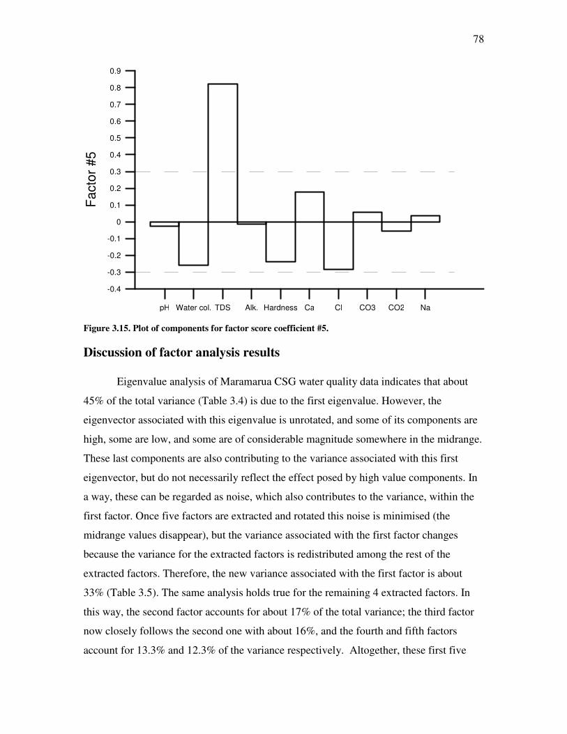
78
pH Water col. TDS Alk. Hardness Ca Cl CO3 CO2 Na
-0.4
-0.3
-0.2
-0.1
0
0.1
0.2
0.3
0.4
0.5
0.6
0.7
0.8
0.9
Fact
or #
5
Figure 3.15. Plot of components for factor score coefficient #5.
Discussion of factor analysis results
Eigenvalue analysis of Maramarua CSG water quality data indicates that about
45% of the total variance (Table 3.4) is due to the first eigenvalue. However, the
eigenvector associated with this eigenvalue is unrotated, and some of its components are
high, some are low, and some are of considerable magnitude somewhere in the midrange.
These last components are also contributing to the variance associated with this first
eigenvector, but do not necessarily reflect the effect posed by high value components. In
a way, these can be regarded as noise, which also contributes to the variance, within the
first factor. Once five factors are extracted and rotated this noise is minimised (the
midrange values disappear), but the variance associated with the first factor changes
because the variance for the extracted factors is redistributed among the rest of the
extracted factors. Therefore, the new variance associated with the first factor is about
33% (Table 3.5). The same analysis holds true for the remaining 4 extracted factors. In
this way, the second factor accounts for about 17% of the total variance; the third factor
now closely follows the second one with about 16%, and the fourth and fifth factors
account for 13.3% and 12.3% of the variance respectively. Altogether, these first five

79
factors still account for 90.9% of the total variance. The analysis of the factor score
coefficients is carried out by examining the significant factor components within each
factor. Even though factor rotation minimises midrange values, a value of 0.3 has been
chosen as a cutting value for determining which components are significant within each
factor.
Factor #1
The components of the factor score coefficients for the first factor are distributed
in such a way that only the components for carbon dioxide, pH, water column, and
carbonate (in order of importance) are significant (i.e. > + 0.3 or < - 0,3; Figure 3.11).
This figure indicates that a strong decrease in carbon dioxide tends to be associated with
a significant decrease in water column together with a considerable increase in pH and
carbonate concentrations. This description fits the carbonate speciation model described
by solving the carbonate equilibrium equations as stated in Snoeyink (1980) and Freeze
(1979). If the carbonate equilibrium equations (Figure 3.16) are solved for different pH
values assuming a total inorganic carbon content of 1M, then the resulting carbonate
speciation plot will be the one presented in Figure 3.17. This plot shows that, for pH
values greater than 7, carbonate concentrations tend to increase with increasing pH values
while carbon dioxide concentrations tend to decrease. Therefore, the first factor score
coefficient represents changes in pH values resulting from the carbon dioxide degassing
process.
][][][
10
,
][][][2][
][][][
10
10
)(232*32
8.232)(22
233
*323
23,
3.10233
3.63
*32
3
aq
aq
COT
COCOHCOH
KCOHCOOH
Where
HOHCOHCOAlkalinity
COHHCOCOC
KCOHHCO
KHCOHCOH
+=
=⇔+
−++=
++=
=+⇔
=+⇔
−
+−−−
−−
−−+−
−−+
Figure 3.16. Carbonate equilibrium equations at standard conditions (Snoeyink and Jenkins, 1980).
80
Solving the carbonate system of equations (Figure 3.16) can help describe the
degassing process. This system was solved using activity coefficients calculated from
ionic strength effects estimated by taking into account specific conductance values
(Appendix A). The lowest pH value detected in the Maramarua CSG water samples was
7.2 (25/04/2005), so pH values in the aquifer have to be less than or equal to this value
because as carbon dioxide concentrations increase (due to higher CO2 pressure in the
aquifer) pH values decrease (Figure 3.17). If the carbonate equilibrium equations are
solved with a pH of 7.2 then the calculated aquifer CO2 pressure is 0.026 atm. Once this
water is exposed to the surface, the pressure drops to normal levels (10-3.5 atm at standard
conditions) and the calculated pH is 9.1. However, these changes do not occur
instantaneously as revealed by the different pH values in the Maramarua CSG water
quality data. As the well is dewatered, different samples are collected under different
degassing and agitation conditions. This water may remain inside the well for a certain
amount of time before it is collected (different water levels), and this also induces
degassing and different qualities of water. On the other hand, degassing can be caused by
water agitation inside the well which occurs when the pump is operating, hence the
negative value for the water column component. Even when the sample is in a bottle,
CO2 degassing, carbonate precipitation, and a rise in pH may still take place if there is a
gap and enough time for the carbon dioxide to escape. Consequently, the first factor
shows that about 33% of the variations are due to this degassing process either during
sampling or subsequently during sampling storage and handling.

81
0.00
0.20
0.40
0.60
0.80
1.00
1 2 3 4 5 6 7 8 9 10 11 12 13 14
pH
mol
es/l
Bicarbonate Carbonate Carbon dioxide
Figure 3.17. Distribution of major species of dissolved inorganic carbon Factor #2
The major components in the second factor, which accounts for 16.5% of the
variance, are sodium, alkalinity (equivalent to bicarbonate for the studied pH range),
water column, and chloride (Figure 3.12). These ions happen to be the major ions in the
samples (water of the Na-HCO3-Cl type as illustrated in Figure 3.6), so this factor is
showing the correlation between the ionic strength of the samples (due to its major ions)
and the water column inside the well. A low water column would indicate that the
pumping process is continuous and there is a low retention time in the vicinity of the well
(this area would be susceptible to erosion/dilution). As a result, the CSG water pumped
out of the aquifer would be less mineralised than the water pumped out of the well after a
long period of exposure in the vicinity of the well; this situation would originate with
discontinuous pumping, low pumping rate, or after a long standby period (high water
column). As dewatering progresses with time, the loose formations around the vicinity of
the well become less prone to dilution (because they have already been exhausted), and
the end result is a slightly less mineralised water. This can be observed with sodium and
bicarbonate concentrations during the first pumping round (Figure 3.9) as concentrations
decrease in a logarithmic (1/ln(x)) fashion. It is not possible to observe this with chloride
because its concentrations stay fairly constant with fluctuations through out time
independently of pumping (Figure 3.9).
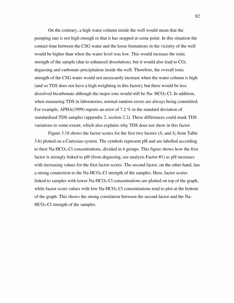
82
On the contrary, a high water column inside the well would mean that the
pumping rate is not high enough or that it has stopped at some point. In this situation the
contact time between the CSG water and the loose formations in the vicinity of the well
would be higher than when the water level was low. This would increase the ionic
strength of the sample (due to enhanced dissolution), but it would also lead to CO2
degassing and carbonate precipitation inside the well. Therefore, the overall ionic
strength of the CSG water would not necessarily increase when the water column is high
(and so TDS does not have a high weighting in this factor), but there would be less
dissolved bicarbonate although the major ions would still be Na- HCO3-Cl. In addition,
when measuring TDS in laboratories, normal random errors are always being committed.
For example, APHA(1999) reports an error of 7.2 % in the standard deviation of
standardised TDS samples (appendix 2, section 2.2). These differences could mask TDS
variations to some extent, which also explains why TDS does not show in this factor.
Figure 3.18 shows the factor scores for the first two factors (S1 and S2 from Table
3.6) plotted on a Cartesian system. The symbols represent pH and are labelled according
to their Na-HCO3-Cl concentrations, divided in 4 groups. This figure shows how the first
factor is strongly linked to pH (from degassing, see analysis Factor #1) as pH increases
with increasing values for the first factor scores. The second factor, on the other hand, has
a strong connection to the Na-HCO3-Cl strength of the samples. Here, factor scores
linked to samples with lower Na-HCO3-Cl concentrations are plotted on top of the graph,
while factor score values with low Na-HCO3-Cl concentrations tend to plot at the bottom
of the graph. This shows the strong correlation between the second factor and the Na-
HCO3-Cl strength of the samples.
83
Legend
Na-HCO -Cl classes (meq/l):3
1) [Na] + [HCO ] + [Cl] 25.02) 25.1 < [Na] + [HCO ] + [Cl] 25.53) 25.6 < [Na] + [HCO ] + [Cl] 26.04) 26.1 < [Na] + [HCO ] + [Cl]
3
3
3
3
≤≤≤
Figure 3.18. Plot of factor scores for the first two factors. Factor #3
The third factor has a similar variance contribution than the second one because it
amounts to 16.0% of the variance (just 0.5% less than the second factor). This factor
shows a negative correlation between chloride and water column. This complements the
interpretation of the second factor which showed a positive correlation between chloride
and water column indicating that chloride is the third major ion present in CSG samples.
However, in the case of the third factor, the negative correlation between chloride and
water column would indicate that chloride concentrations are high with water column
decline. Therefore, the second and third factors indicate that chloride concentrations are
fairly independent of water levels inside the well - where factor #2 shows a positive
correlation with water levels, factor #3 shows a negative one. In this way, chloride
concentrations tend to remain constant throughout dewatering (the relative standard
deviation of the 31 samples is 1.8%).

84
Factor #4 Factor #4 shows a strong correlation between calcium and hardness. This is not
unexpected as the value for hardness includes the value for calcium plus the value for
magnesium. Therefore, a strong change in calcium concentrations would cause a change
in hardness. The calcium coefficient for this factor is more heavily weighted than the
hardness one (which also includes magnesium), so calcium is the main source of
variation associated with this component. Calcium concentrations could vary
significantly with calcium carbonate precipitation, which occurs with CSG water
degassing. However, factor #4 does not include heavily weighted coefficients for any of
the components associated with calcium carbonate precipitation (pH, water column,
carbonate, and carbon dioxide). Since there are no other high-value coefficients for this
factor, the calcium variation could be attributed to the analytical determination of calcium.
APHA reports a RSD of 9.2% associated with this technique, but laboratory titrations
conducted at the EEL could have been as high as 17.3% (Appendix B, section B.2).
Factor #5
In factor #5 the only significant component is TDS. Therefore, this factor
represents an independent source of variation associated with the TDS content of the
Maramarua CSG water samples. This variation would be linked to the analytical
technique used to measure TDS rather than to an actual process in the aquifer or in the
well. This is because one would expect a strong correspondence between TDS and the
coefficients for the major ions present in the samples (Na-HCO3-Cl), but these
coefficients are too low for factor #5. In the analytical determination of TDS sometimes
there are significant differences in results because the reaction which dissociates
bicarbonate into carbonate, carbon dioxide, and water may not always reach completion
(Appendix B, section B.2). As mentioned in factor #2, the relative error of this technique
could be as high as 7.2%, so there is a high uncertainty surrounding TDS determinations.
Consequently, factor #5, which represents 12.3% of the variance, most likely represents
the uncertainty associated with this measuring procedure.

85
Table 3.7. Summary of factor score coefficients reification Factor # Total variance
contribution (%)
Processes or analytes responsible for this contribution
1 32.8% o Carbon dioxide degassing process 2 16.5% o Relationship between major ion composition (Na-
HCO3-Cl) and water column decline 3 16.0% o Chloride variation in the well independent of water
level 4 13.3% o Calcium variations due to errors in analytical
determination 5 12.3% o Variations attributed to analytical method for
determining TDS
Table 3.7 summarises the reification of the Maramarua C-1 CSG water factors.
Water abstracted from this well exhibits basically the same chemical characteristics and
concentrations throughout different samples, but with minor variations. Factor analysis of
these data has revealed that the majority of these variations (about 33%) are due to
carbon dioxide coming out of solution and escaping into the atmosphere. This takes place
either inside the well or later with sample handling. The second source of variation
(16.5%) is linked to an increase in ionic strength due to changes in pumping rate which
may affect dissolution in the vicinity of the well. The third factor (16%) shows that
chloride concentrations are independent of water level inside the well. Lastly, factors 4
(13.3%) and 5 (12.3%) both relate to a systematic form of variation associated with the
analytical determination of calcium and TDS respectively. Since the main source of
variation is due to CSG water degassing, it would help to verify this conclusion with a
laboratory experiment.
Degassing investigation analysis
The aim of this degassing investigation work was to verify the factor analysis
results- carbon dioxide degassing and carbonate speciation (factor #1), which were
responsible for about one third of the total variance (32.8%). For this purpose both a
practical and theoretical investigation were carried out. The practical experiment used
actual CSG water, while the theoretical one used a chemical speciation model, Visual
MINTEQ, and sample analysis results.

86
Methods
Practical experiment A practical experiment was set up with actual Maramarua CSG water. The experiment
consisted of selecting a recently collected sample (11/06/2005) and very carefully
(avoiding unnecessary agitation) measuring its key chemical properties – specific
conductance, alkalinity, pH, hardness, and calcium. Special provisions were made to
measure calcium and hardness – samples were centrifuged and filtered (using 0.22 µm
filters) to ensure that only diluted ions were measured. A certain volume (1.5 L) of water
was placed in a 2 L Erlenmeyer flask. The flask and the water were weighed and the
measurement recorded. A porous hollow coil was then introduced inside the flask, and air
was continuously pumped through it, generating bubbles in the water. A picture of this
experimental setup is presented in Figure 3.19. The principle in this experiment is to
generate air bubbles in order to cause agitation and accelerate the carbon dioxide
degassing process. While this was carried out, a “cold finger”, which was basically an
open glass column with an inner glass coil with circulating cold water, was introduced
into the system to a level just above the water mark. This cold finger acted as a trap for
water vapour leaving the system. Water particles leaving the system would condense on
the cold finger and would slowly drip back into the sample. The opening on top of the
flask was wrapped with plastic around the cold finger to avoid losses. This sparging
experiment was run for 6 hours at a temperature of about 20°C. After this time, the flask
was weighed again and the water specific conductance was recorded. Any discrepancies
due mainly to water vapour escaping the system were corrected by adding deionised
water until the original weight and specific conductance were achieved (there was a loss
of 5.57 ml of water). It was assumed that the effects of carbon dioxide degassing on
weight and specific conductance were negligible, and this was later confirmed with
calculations indicating carbon dioxide differences posing no effects in relation to these
variables (Table 3.10). Once the sample had been corrected, the sparged CSG water was
analysed to obtain the same key chemical properties measured before sparging. �

87
Figure 3.19. Sparging of CSG water
Theoretical experiment The theoretical experiment consisted of modelling the practical experiment using
a chemical speciation model, Visual MINTEQ. This model is a Visual Basic version of
the EPA MINTEQA2 v. 4.0 model, which is a chemical speciation model designed to
calculate the equilibrium composition of aqueous solutions (US Environmental
Protection Agency, 2005). A complete Maramarua CSG water sample analysis taken on
19/8/2004 was used as input for the model both with its original pH, and with the final
pH at the end of the sparging experiment. The equilibrated mass distribution resulting
from running the model was noted and its results were compared against the sparging
results.
Experimental results
Results for the practical experiment are presented in Table 3.8. Once the sparging
was over, the water was left undisturbed for about 8 hours on a closed container. After
this period of time large light grey fragments were observed at the bottom of the bottle.

88
The sample was corrected by adding deionised water to account for water losses through
evaporation (0.26%). Initial and final conditions after sparging differ mainly in pH,
hardness, and calcium.
Table 3.8. Results of sparging experiment Parameters Units initial conditions after sparging pH pH units 7.4 8.6 Specific Conductance µS/cm 1314 1315 Alkalinity As mg/l CaCO3 380 380 Hardness As mg/l CaCO3 22.3 14.7 Calcium mg/l 4.8 2.9 Magnesium mg/l 2.5(1) 1.9(1) Weight (water+flask) grams 2136.88 2136.84(2) (1) Calculated from hardness and calcium concentrations
(2) Value corrected with deionised water. Original value was 2131.31g (0.26% loss) Sample was sparged for 6 hours at a temperature of 19.5°C
Results from the theoretical experiment using the Visual MINTEQ model are
presented in Table 3.9. The original sample had a pH of 7.8 and, according to MINTEQ,
presented some carbonate and zinc precipitation in the form of smithsonite. However,
zinc precipitation for this pH value could be virtually nonexistent because the saturation
index for zinc (calculated with MINTEQ) is zero for smithsonite (ZnCO3), and the rest of
the minerals are undersaturated. On the other hand, smithsonite and calcite precipitation
are significant when running the model with a pH of 8.6, which corresponds to the pH of
the 11/06/2005 sample after the sparging experiment. Under these conditions, the
calculated saturation index for smithsonite continues to be zero, but could have had a
larger value before zinc precipitation took place. The calcite saturation index is 0.003,
which means the solution is oversaturated with respect to calcite and will tend to
precipitate this mineral.

89
Table 3.9. MINTEQ modelling results Modelling of 19/8/2004 sample with original pH (7.8) ��= 0.9989 kg/l�Parameter total dissolved
moles/kg %dissolved total precipitated
moles/kg % precipitated
Barium 1.4562�10-7 100 0 0 Calcium 1.4970�10-4 100 0 0 Chloride 4.1181�10-3 100 0 0 Carbonate 7.4015�10-3 99.766 1.74�10-5 0.234(1) Fluoride 4.1582�10-5 100 0 0 Potassium 7.6722�10-5 100 0 0 Magnesium 3.7019�10-5 100 0 0 Sodium 1.4528�10-2 100 0 0 Sulphate 7.2870�10-6 100 0 0 Zinc 2.1972�10-6 11.221 1.74�10-5 88.779(1) Modelling of 19/8/2004 sample with sparging experiment pH (8.6) ��= 0.9973 kg/l Parameter total dissolved
moles/kg %dissolved total precipitated
moles/kg % precipitated
Barium 1.4562�10-7� 100 0 0
Calcium 6.5374�10-5 43.67 8.43�10-5 56.33(2) Chloride 4.1181�10-3 100 0 0 Carbonate 7.0936�10-3 98.58 1.03�10-4 1.425(1,2) Fluoride 4.1582�10-5 100 0 0 Potassium 7.6722�10-5 100 0 0 Magnesium 3.7019�10-5 100 0 0 Sodium 1.4528�10-2 100 0 0 Sulphate 7.2870�10-6 100 0 0 Zinc 1.3288�10-6 6.79 1.83�10-5 93.214(1) (1)Precipitates as smithsonite (ZnCO3) (2)Precipitates as calcite (CaCO3) Note: Liquid density changes as minerals precipitate from solution. Therfore, C (moles/l) = C(moles/kg) * ��(kg/l)
In addition, MINTEQ was run a few more times but with pH values of 8.9 and 6.6
to predict what minerals could precipitate out under these conditions. When running the
model with a pH of 8.9, the saturation index for calcite remained at 0.003, but this time
dolomite (Mg CO3) and hydrozincite reached equilibrium with a saturation index of zero.
Consequently, calcium, magnesium, carbonate and zinc precipitated out of solution.
Finally, successive model executions using decreasing pH values revealed that at a pH of
6.6, smithsonite became undersaturated with respect to carbonate and no precipitation
took place.
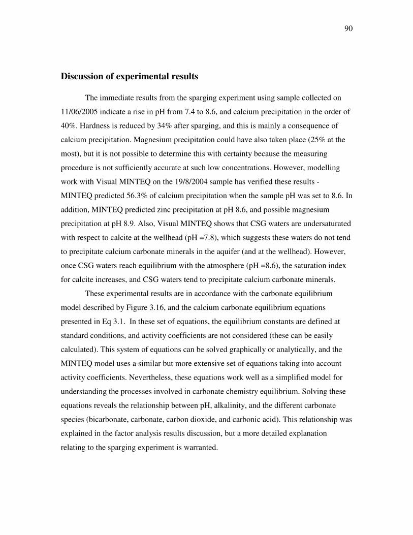
90
Discussion of experimental results
The immediate results from the sparging experiment using sample collected on
11/06/2005 indicate a rise in pH from 7.4 to 8.6, and calcium precipitation in the order of
40%. Hardness is reduced by 34% after sparging, and this is mainly a consequence of
calcium precipitation. Magnesium precipitation could have also taken place (25% at the
most), but it is not possible to determine this with certainty because the measuring
procedure is not sufficiently accurate at such low concentrations. However, modelling
work with Visual MINTEQ on the 19/8/2004 sample has verified these results -
MINTEQ predicted 56.3% of calcium precipitation when the sample pH was set to 8.6. In
addition, MINTEQ predicted zinc precipitation at pH 8.6, and possible magnesium
precipitation at pH 8.9. Also, Visual MINTEQ shows that CSG waters are undersaturated
with respect to calcite at the wellhead (pH =7.8), which suggests these waters do not tend
to precipitate calcium carbonate minerals in the aquifer (and at the wellhead). However,
once CSG waters reach equilibrium with the atmosphere (pH =8.6), the saturation index
for calcite increases, and CSG waters tend to precipitate calcium carbonate minerals.
These experimental results are in accordance with the carbonate equilibrium
model described by Figure 3.16, and the calcium carbonate equilibrium equations
presented in Eq 3.1. In these set of equations, the equilibrium constants are defined at
standard conditions, and activity coefficients are not considered (these can be easily
calculated). This system of equations can be solved graphically or analytically, and the
MINTEQ model uses a similar but more extensive set of equations taking into account
activity coefficients. Nevertheless, these equations work well as a simplified model for
understanding the processes involved in carbonate chemistry equilibrium. Solving these
equations reveals the relationship between pH, alkalinity, and the different carbonate
species (bicarbonate, carbonate, carbon dioxide, and carbonic acid). This relationship was
explained in the factor analysis results discussion, but a more detailed explanation
relating to the sparging experiment is warranted.

91
)(3..
1010
3.10
3.8
32
)(3
sCaCOwithmequilibriuinwater
s
pHpHIS
KHCOCaHCaCO
−=
=+⇔+ −
−−++
Eq 3.1
When CSG waters are in the aquifer, the partial pressure of carbon dioxide can be
up to two orders of magnitude greater than at the surface. In this case, the carbonate
system behaves as a closed system with a constant elevated partial pressure of carbon
dioxide. At this pressure, some carbon dioxide will remain dissolved in the water, and the
only other carbonate species present will be bicarbonate. Furthermore, CSG waters will
be completely undersaturated - according to MINTEQ modelling, this could occur at pH
6.6 because at this pH value smithsonite (ZnCO3) remains completely dissolved in the
aquifer. However, once CSG waters are pumped to the surface, these waters are exposed
to a much lower atmospheric pressure; carbon dioxide gas will come out of solution and
their carbonate equilibrium will start to change. Unless special provisions are taken (like
the use of micropurge sampling and cell flows) it is practically impossible to avoid the
degassing process.
The sample collected on 11/06/2005 from the Maramarua C-1 well had already
lost some carbon dioxide, and its pH (7.4) was already higher than aquifer pH. However,
because this sample was stored in a closed plastic bottle which had been completely filled
with CSG water (leaving no air gaps), the degassing effect was somehow controlled. The
carbonate species and properties for this sample are presented in Table 3.10. Before
sparging, the major ion of the carbonate species was bicarbonate (462 mg/l) followed by
dissolved carbon dioxide (62 mg/l). The calculated saturation index for this sample is
negative (-0.95) which means this sample is not precipitating calcium carbonate. Once
the sample was sparged, the carbon dioxide degassing process was accelerated because
the sample was exposed to the open atmosphere and to a lower atmospheric pressure. As
a consequence, the pH rose from 7.4 to 8.6, and the carbonate equilibrium changed
(Table 3.10). This time, dissolved carbon dioxide concentrations were very low (3.7
mg/l), and carbonate concentrations increased to 12 mg/l; the major carbonate ion
continued to be bicarbonate, but its concentration decreased to 438 mg/l. In general, these

92
results can be interpreted graphically using Figure 3.17. This figure shows how carbon
dioxide decreases while carbonate increases as pH values increase. Bicarbonate may
reach a maximum at pH 8.3, but it then starts to decrease with increasing pH values. The
sparged Maramarua 11/06/2005 sample has a pH of 8.6, therefore bicarbonate
concentrations for this sample must have increased to a maximum at pH 8.3 (starting at
pH 7.4), and then decreased to 438 mg/l with a final pH of 8.6.
Another significant consequence resulting from sample sparging is the saturation
index, which in this case resulted in a positive value (0.29). This value is close to zero
because most of the calcite has precipitated (it must have been higher at some point but
then decreased as calcite precipitated). This was verified by measuring calcium
concentrations before and after sparging with differences of 40%. In addition, MINTEQ
modelling with the full 19/8/2004 sample analysis results has resulted in a positive
saturation index (0.003), which also helps to corroborate the calculated value for the
11/06/2005 sample (0.29).
Table 3.10. Carbonate species and properties for 11/06/2005 sample Carbonate species or property units before sparging after sparging pH pH units 7.4 8.6 HCO3
- mg/l 461.5 437.7 CO3
2- mg/l 0.8 12.4 CO2 (aq) mg/l 61.7 3.7 H2CO3 mg/l 0.098 0.006 H2CO3
* mg/l 61.8 3.7 Saturation Index pH units -0.95 0.26 Notes: The different carbonate species were calculated using Figure 3.16 with activity coefficients, and an alkalinity of 380 as mg/l CaCO3 The Saturation Index (or Langelier Index) was calculated by the difference between the actual water pH and the pH of water in equilibrium with CaCO3 (Eq 3.1).
In the factor analysis, it was possible to correlate the carbonate precipitation
process to water levels fluctuations. Higher levels would imply that the water has been in
the well for a longer time. Therefore, higher water levels would expose CSG water to a
lower atmospheric pressure, and the degassing/precipitation process would be promoted.
Aquifer pH could be as low as 6.6 because at this pH value, MINTEQ predicts no solid
precipitation. However, when CSG water is abstracted, its pH inside the well
immediately begins to rise because of the pressure difference. When the sample is

93
collected pH could rise further with agitation and sample handling. For example, the full
sample collected on the 19/08/2004 had a pH of 7.8. The difference between this pH
value and the pH of the water in the aquifer (6.6) is high (1.2 units), and it represents the
amount of degassing that has taken place.
Alkalinity before and after sparging did not change (Table 3.8). Once again, this
result is entirely expected according to carbonate equilibrium (Figure 3.16); in this
system of equations, the concentration of the different carbonate species can be
calculated if pH and alkalinity are known. By using Figure 3.16, it is possible to verify
that the addition or removal of carbon dioxide does not influence the final alkalinity value,
and this confirms the experimental result in Table 3.8. This result has further implications
for sampling CSG waters – when sampling, it would be ideal to measure pH at the
wellhead because this value changes with degassing. Samples can be analysed for
alkalinity at a later stage in the lab since this value will not change as carbon dioxide is
lost.
MINTEQ modelling revealed that degassing is likely to cause calcium
precipitation as calcium carbonate (CaCO3) and zinc precipitation as smithsonite
(ZnCO3). Most likely, the grey coloured precipitate, formed after sparging the 11/06/2005
sample, could have included both calcium carbonate and smithsonite. According to
MINTEQ, zinc precipitation could be as high as 93% and, in the case of the 19/8/2004
sample which had a zinc concentration of 1.28 mg/l this could represent a significant
reduction (0.09 mg/l) if the CSG water is exposed to the open atmosphere for some
period of time. For example, it could be desired to precipitate zinc in a pond prior to
discharge; this would effectively reduce zinc concentrations in the CSG water, but would
result in a sludge with high zinc concentrations which would have to be properly handled.

94
Conclusion
A CSG dewatering operation in Maramarua has produced a set of water samples
with some minor variations in chemical composition. The setup was ideal for this purpose,
because the samples were abstracted as the well was subjected to intermittent and
continuous dewatering with two different pumps. Consequently, the resulting data set
permitted studying the causes of variation in water quality while considering obvious
changes throughout the dewatering process (water level fluctuations).
A factor analysis has unveiled calcium carbonate precipitation with carbon
dioxide degassing as the number one cause of variation (32.8%). This is significant
because all CSG aquifers have high bicarbonate concentrations, and are located at depths
associated with high aquifer pressure. Therefore, all CSG waters are highly sensitive to
variations due to internal changes in their carbonate equilibrium arising from changes in
the pressure to which they are subjected. These variations can be minimised if samples
are collected with minimum disturbance, and if provisions are taken to prevent carbon
dioxide gas from coming out of solution once the sample is collected. Higher variations
are expected if the sample is exposed to the open atmosphere for a prolonged period of
time or has undergone violent agitation. This was verified experimentally with a sparging
experiment and subsequent modelling work. A recommendation from these findings is to
sample CSG waters on site by measuring pH and avoiding degassing as much as possible.
It is not necessary to measure alkalinity on site since this value will not change with
degassing.
The second source of variation is related to the major ion composition (Na-HCO3-
Cl) of CSG waters. Factor analysis results indicated that about 16.5% of the variance is
due to the relationship between sample mineralization and water column. This could
reflect the influence pumping has on the dissolution of minerals present in formations
near the well. The third factor (16% of variation) shows the negative correlation between
chloride and water level, which complements the positive correlation found in the second
factor, and suggests chloride concentrations are fairly independent of water level. The
fourth (13.3% of variation) and fifth (12.3% of variation) factors are linked to measuring
errors that could have been committed when determining calcium and TDS

95
concentrations respectively. It was possible to verify the interpretation of the first factor
(which is the most important one) using an experimental setup and further theoretical
modelling - it was not possible to verify the interpretation of the rest of the factors, but
these factors are not as relevant as factor #1.
CSG waters from Maramarua C-1 have a high bicarbonate concentration, which
plays an important role in shaping their quality once abstracted; this makes these waters
extremely unstable once pumped to the surface. An initial inspection might give the
impression of these waters being chemically stagnant, however a closer examination
reveals that, once exposed to surface atmospheric pressure, these waters have the
potential to precipitate calcium, zinc, and magnesium in carbonate form. In addition, pH
rises considerably, but bicarbonate concentrations decrease slightly while small amounts
of carbon dioxide gas are vented. Consequently, different pumping rates, along with
changes in pressure, will produce a continuously changing water quality. Indeed, as
Heraclitus put it, the nature of water flow is constant change - this applies to all sorts of
water bodies, even the ones taking place underground (aquifers). Although factor analysis
results, sparging experiments, and MINTEQ modelling are in accordance with each other
and yield similar inferences, this research would have benefited from replicates and tests
on other water samples to give confidence to these conclusions.

96
References American Public Health Association., American Water Works Association., and Water
Environment Federation., 1999, Standard methods for the examination of water
and wastewater: [Washington, D.C.], American Public Health Association, 1
computer optical disc p.
Chatfield, C., 1996, The analysis of time series : an introduction: London, Chapman &
Hall, xii, 283 p.
Davis, J.C., 2002, Statistics and data analysis in geology: New York, J. Wiley, xvi, 638 p.
p.
Freeze, R.A., and Cherry, J.A., 1979, Groundwater: Englewood Cliffs, N.J., Prentice-Hall,
xvi, 604 p.
Hoffman, R.D., and Animated Software Company., 2004, Internet glossary of pumps:
[California], Animated Software Co.
Karassik, I.J., 1986, Pump handbook: New York, McGraw-Hill, 1 v. (various pagings) p.
Nielsen, D., 1990, Practical handbook of ground-water monitoring: Chelsea, MI, Lewis
Publishers, x, 717 p.
Snoeyink, V.L., and Jenkins, D., 1980, Water chemistry: New York, Wiley, xiii, 463 p.
US Environmental Protection Agency, 2005, Exposure Assessment Models, US
Environmental Protection Agency, p. web page.
Van Voast, W.A., 2003, Geochemical signature of formation waters associated with
coalbed methane: Aapg Bulletin, v. 87, p. 667-676.

97
4. Chapter 4
Potential environmental impacts associated with coal seam gas water management in New Zealand
Introduction
The environmental impacts that could arise from CSG water extraction depend on
the quantity and quality of produced water, and on the method of treatment and disposal
being used. For example, if CSG waters are disposed of on the land, the main impacts
would be on plant development and soil stability, whereas if these waters are disposed of
on rivers, the impacts would be on aquatic life. Understanding these impacts is necessary
to adequately manage CSG waters so that environmental effects are minimised; if
properly managed, CSG waters can be used for beneficial applications and can become a
valuable resource.
In the United States, impacts associated with CSG water discharge have been
noted in the Powder River Basin (PRB) and have been reported by Bauder (2001),
Wheaton and Donato (2004), McBeth et al. (2003), and Davis et al. (2006b). However, in
other CSG producing basins in the US (San Juan, Raton, Uinta) impacts have been
minimal because the lower volumes of water being produced have allowed injection into
receiving aquifers as the main method of disposal (ALL-Consulting and Montana Board
of Oil and Gas Conservation, 2004). Similarly, producers in the Black Warrior Basin in
Alabama have successfully treated their low-volume CSG water by directing it through a
sequence of treatment/storage ponds in order to discharge it into surface streams (Davis
et al., 1993). All of these disposal methods have had to comply with US regulations
(National Pollutant Discharge Elimination Permits) to minimise potential impacts at a
reasonable price.

98
Although CSG water tends to have the same major ion composition throughout
different basins (Van Voast, 2003), the magnitude of potential environmental impacts
change across basins due to differences in local climate, receiving soils, surface waters,
and quantities of CSG water being abstracted. This chapter outlines the potential
environmental problems associated with CSG waters in New Zealand while considering
overseas experience. In this context, the New Zealand regulatory framework is explained,
and management options are outlined. This chapter explains the potential environmental
impacts associated with CSG water disposal in New Zealand. Other impacts not directly
related to CSG water (i.e. noise, land or scenery disturbance, and air pollution) are not the
focus of this study, but would need adequate characterisation for a complete assessment
of environmental effects from the regulatory point of view. Such an assessment, for
example, would depend on the specific details for each particular operation including
location, dewatering method, and proximity to populated centres. The chapter finishes
with a New Zealand case study of the Maramarua basin.
Assessing environmental impacts related to CSG water management and disposal
CSG waters, as described in Chapter 2, can be detrimental to receiving
environments mainly because of the high sodium, chloride, and bicarbonate
concentrations associated with their geochemical signature. Other issues to consider are
water pH, salinity (specific conductance), and boron (when present). Trace elements
detected in PRB CSG water include barium, arsenic, aluminium, iron, selenium, fluoride,
copper, molybdenum, manganese, chromium, and zinc (McBeth et al., 2003). In addition,
well stimulation techniques could include the injection of sand and fluids to open cleats
and promote gas desorption and transport; these fluids can range from water based to
biodegradable compounds, and the latter could result in CSG water having high BOD
during the first months of dewatering (Davis et al., 1993). The problem ceases to become
a pure CSG project if the CSG has been exposed to secondary processes such as, for
example, the mixing with heavier hydrocarbons from conventional natural gas linked to
oil production (Rice, 1993). In these situations trace elements like iron, manganese, and
organics could be present in higher concentrations (Davis et al., 1993).

99
The impacts associated with CSG water disposal depend on the method of
disposal being implemented. The major disposal options are discharge to land and surface
waters; the impacts for each of these receiving environments will be different and need to
be assessed before disposal is implemented. In general the longer the path from the
discharge point, the larger the potential for environmental damage. The situation becomes
complicated when valuable resources are compromised (fertile soils, pristine aquifers,
rivers, and wetlands), and when there are unpredictable links between receiving
environments (i.e. aquifer interconnection or runoff to recharge areas). Therefore, each
disposal option and its impacts needs to be properly assessed before it can be
implemented.
In New Zealand, the Resource Management Act (RMA) is the main legistation
controlling contaminant discharges into the environment. It is the role of regional
councils to implement the RMA by issuing regional policy statements and implementing
regional plans. Proposed activities have to undergo a thorough consent process and, to aid
in their decisions, regional councils may rely on various New Zealand guidelines. If no
local guidelines are available, overseas guidelines may be employed or site-specific
guideline values may be developed (Cavanagh and Coakley, 2005). Full-scale CSG
production has not yet taken place in New Zealand, and the effects associated with CSG
water discharge are generally unknown. Therefore, regional councils have not yet had to
assess resource consents for large CSG mining activities, which involve CSG water
disposal.
Land disposal of CSG waters
Land disposal of CSG waters can have different impacts depending on whether
these waters are being disposed directly on to the land or used for irrigation of fertile soils.
The major issues with CSG water are its salinity (specific conductance) and its major ions
(sodium and chloride) which can be toxic to plants and may damage the permeability of
soils (i.e. high Exchangeable Sodium Percentage or ESP levels). Salinity is generally
measured in dS/m units, however in previous chapters it has been reported as µS/cm to
show all significant figures (1 dS/m = 1000 µS/cm). In this chapter, salinity will be
reported as dS/m to allow for a direct comparison between selected samples and salinity

100
values in various irrigation water quality guidelines, which are used in assessing salinity
problems associated with land disposal of CSG waters.
High salinity can have a detrimental effect on vegetation because plants need to
exert extra osmotic force to extract water from the soil-water interface (Ayers et al.,
1985). With increasing salinity levels, plant growth is suppressed and, at critical levels,
plants can die (Jensen, 1983). Some plants are more tolerant to salinity than others. For
example, barley has a 100% tolerance to salinity levels of 5.3 dS/m, while carrots have a
100% tolerance at salinities of 0.7 dS/m. In contrast, halophytes, which grow on wetland
environments, can tolerate extremely high saline levels (up to 90 dS/m) (Settle et al.,
1998). For agricultural applications, salinity levels greater than 3 dS/m have been
identified as “severe” by Ayers et al. (1985).
On the other hand, salinity can play an important role in keeping soil particles
flocculated and maintaining good permeability. Oster and Schroer (1979) observed a
correlation between infiltration rates and total ion concentration (salinity). This
occurrence is explained because, at high salt concentrations, pH values are lower than 8.5
and soil particles tend to remain flocculated (US Salinity Laboratory Staff, 1954). At
lower salinity levels, the soil-water solution may have pH values above 8.5 and the
sodium ions, which were originally part of the soil, can hydrolyze and rearrange clay
particles causing overall soil dispersion and the loss of permeability (US Salinity
Laboratory Staff, 1954).
The high sodium together with low calcium and magnesium concentrations in
CSG waters have the potential to cause soil dispersion and loss of infiltration. The
problem of irrigating soils with saline/sodic water has been studied by US Salinity
Laboratory Staff (1954), Oster and Schroer (1979), and Ayers et al. (1985) among others.
These researchers have developed guidelines to prevent infiltration problems based on
the Sodium Adsorption Ratio (SAR) and salinity of irrigation waters while considering
the ESP of the soil. Using various saline/sodic water combinations on non-saline/non-
sodic loams, Oster and Schroer (1979) showed that infiltration rates decreased as SAR
values increased and salinity decreased. From the soil point of view, an ESP value of 15
has been selected in the US as the limit for soils containing clay minerals to become
degraded (Shainberg and Letey, 1984; US Salinity Laboratory Staff, 1954). A

101
relationship between ESP and SAR has been established relating the ESP value of 15 to a
SAR value of 12.8 for soils in Western States in the US (US Salinity Laboratory Staff,
1954). Research by Robinson (2003) has revealed that continuous cycles of irrigation
with deionised water and synthesized CSG water from the PRB, produces soil
salinisation and potential infiltration problems in PRB soils.
Salinity and infiltration problems due to sodium are complex and need to be
studied within the context of each individual basin. For example, the guidelines by Ayers
et al. (1985) were developed for semi-arid to arid climates on soils with sandy-loam to
clay-loam textural range. Therefore, it is not simple to apply these principles and
guidelines to soils in humid regions, like most of the soils in New Zealand.
New Zealand regions exhibit a wide variation of climates ranging from very dry
climates with poorly leached soils (Alexandra) to humid climates with extremely leached
soils (Hokitika), and New Zealand soils are a consequence of the water balance
throughout these different regions (McLaren and Cameron, 1990). Most of the climates in
New Zealand are humid, and saline soils are practically non existent in humid climates
because salts originally present in soils are leached into the groundwater and are
eventually flushed into the ocean (US Salinity Laboratory Staff, 1954), therefore
salinisation is not a major concern in New Zealand (ANZECC and ARMCANZ, 2000).
Most of the soils in New Zealand are well drained and have moderate (medium) cation
exchange capacities (Figure 4.1), however saline and alkaline soils do exist in some areas
of Central Otago at about 200-600m elevation (Allen et al., 1998).
New Zealand soils tend to have considerable amounts of organic matter
(“Medium” category in Figure 4.2), and Bresler et al. (1982) have suggested that soils
having substantial amounts of organic matter have good water retention ability, are
relatively stable, and not prone to swelling or dispersion. Nevertheless, there is
apprehension in New Zealand about the long term effects of discharging high-SAR/
saline water on to the land. For example, an ESP value of 6 is generally being used in
Resource Consent Applications for approving land treatment of dairy farm effluent which
is high in sodium (Cameron et al., 2003). From the regulatory point of view, regional
councils in New Zealand may use the Australian and New Zealand Guidelines for Fresh
and Marine Water Quality (ANZECC and ARMCANZ, 2000) or other relevant
102
Figure 4.1. Cation exchange capacities for New Zealand soils. Map compiled from Landcare Research New Zealand Ltd (2000b).

103
guidelines (including international guidelines) to assess salinity and infiltration problems
caused by high SAR water discharges. These guidelines do not state specific trigger
values because salinity and sodicity problems need to be assessed for each particular
situation while considering parameters like water quality, soil properties, climate, type of
irrigation, and water management practices (ANZECC and ARMCANZ, 2000).
In New Zealand, sodium-loaded liquid wastes from processing and cleaning are
generally being disposed on farmland as the preferred alternative to surface water
disposal (Menneer et al., 2001). These wastewaters can have high SAR levels, which
could generate infiltration problems, effluent runoff, and ponding (Cameron et al., 2003).
Research by Menneer et al. (2001) and Cameron et al. (2003) has focused on
studying the effects of land disposal of dairy farm effluent on New Zealand soils. Using
repacked soil cores in a laboratory study, Menneer et al. (2001) noticed a decrease in
hydraulic conductivity after irrigating with high-SAR solutions followed by leaching with
deionised water. This reduction occurred at SAR values of 3.5 for Waitoa soils and 8.5
for Te Puninga soils (silt loams with 27% and 21% clay respectively); during SAR
application the infiltration rate was enhanced due to the elevated salinity of the applied
solutions.
Cameron et al. (2003) studied the effects of dairy farm effluent (SAR ~ 8.6)
application on a Lismore soil (stony silt loam) with 0, 4, and 10 years of treatment (0 was
the control). Although the soils that had previously been irrigated with dairy farm effluent
had larger ESP values than the control, these soils showed better wet aggregate stability
and permeability upon continuous treatment with high-SAR solutions. This was
attributed to the high carbon content (lactose) of dairy farm effluent which improved soil
structure by providing bonding agents (Cameron et al., 2003). In addition, it was
suggested that an ESP value of 6 may not be appropriate for these situations because,
even though there might not be infiltration problems during applications (due to high
salinity), a soil with a high ESP value could undergo a loss in permeability upon leaching
with rainfall water.
These findings have great implications for land disposal applications of CSG
waters in New Zealand. Firstly, the control water in the experiment by Cameron et al.
(2003) has a chemistry similar to CSG waters for infiltration analysis purposes, and this

104
Figure 4.2. Organic matter content (as carbon percentage) for New Zealand soils. Map compiled using Landcare Research New Zealand Ltd (2000b)

105
sample showed significant reduction in hydraulic conductivity and wet aggregate stability.
Secondly, CSG waters have low organic carbon concentrations (see Chapter 2) (Taulis et
al., 2005) so their land disposal would not condition soils, as in the case of dairy farm
effluent. Consequently continuous disposal of high-SAR CSG water could produce more
infiltration problems than dairy farm effluent, and these effects would be even more
noticeable after long periods of precipitation.
Figure 4.3 shows the potential infiltration problems that could arise due to the
disposal of high-SAR CSG waters on New Zealand soils. A detailed explanation of the
procedure used to create and calibrate the model for Figure 4.3 is presented in Appendix
C (section C.1.2).
In general, the risks are low to moderate, but some high-risk areas do exist in coastal
areas (South of Thames and Napier) and south mountainous areas (Central Otago). CSG
sites presently under exploration are indicated on the map; in the North Island,
Maramarua is located in an area of moderate risk surrounded by patches of low and high
risk. In the South Island, Ashers-Waituna and Kaitangata are close to the ocean, but
Reefton and Hawkdun are located further inland. Ashers-Waituna is located in an area of
low risk, while Kaitangata is located in an area with patches of low, moderate, and high
risk of dispersion. Reefton is surrounded by low and moderate risk patches, while
Hawkdun is located in an area of moderate risk with low to high risk areas downstream
from its location. In general, Figure 4.3 gives a good indication of the infiltration
problems on soils that could arise due to high-SAR water disposal. However, this model
is useful only for general assessments, and more detailed studies should rely on actual
field sample analyses.

106
Figure 4.3. Infiltration problem potential for New Zealand soils exposed to high-SAR water for prolonged periods of time. Model produced using the FSDL (Landcare Research New Zealand Ltd, 2000b) and assumptions in Appendix C.

107
In addition to salinity and infiltration problems, CSG waters can generate other problems
when carrying out land disposal applications. CSG waters generally contain high sodium and
chloride concentrations which pose specific ion toxicity issues when used for crop irrigation.
Toxicity effects from sodium and chloride include leaf burn, scorch and dying of leaf tissue, and
in time these effects may significantly reduce crop yield (Ayers et al., 1985). In some instances,
CSG waters may also contain appreciable quantities of boron (Taulis et al., 2005), which may
cause a toxicity hazard (Ayers et al., 1985). Another trace element to consider is zinc, which has
the potential to accumulate in soils thus becoming present in plant tissue and causing significant
growth reduction. However, zinc poses a reduced toxicity risk for plants (Ayers et al., 1985)
because of the high pH (> 6) of CSG waters which constraints zinc accumulation on soils,. In
addition to zinc, CSG waters from other basins in New Zealand could have other trace elements
depending on specific aquifer characteristics, therefore sample collection and water
characterisation at each site is important to determine the range of trace elements that could be
present.
If sprinkler irrigation is used, the toxicity is aggravated because toxic ions are absorbed
through leaves hit by sprinkler water (Ayers et al., 1985). Toxicity guidelines which would apply
to CSG waters when used in irrigation applications are presented in Table 4.1. Less stringent but
more crop-specific toxicity trigger values are presented in the Australian and New Zealand
Guidelines for Fresh and Marine Water Quality (ANZECC and ARMCANZ, 2000). In addition,
with land application of CSG water there could be indirect toxicity problems arising from the
mobilisation of certain trace elements in the soil. For example, McBeth et al (2003) have
suggested that arsenic, selenium, and fluorine could become soluble and mobile in soils irrigated
with CSG water. This can take place because these ions form anionic species with soil particles,
and can become soluble when soils are irrigated with alkaline waters (McBeth et al., 2003).
However, New Zealand soils are generally low in selenium, which is a dietary supplement in
New Zealand, so increased selenium mobility could prove beneficial in some instances.
Table 4.1. Toxicity guidelines for managing water quality issues relating to irrigation applications1 Specific ion toxicity Units Degree of restriction on use None Slight to moderate Severe Sodium (Na+)
Surface irrigation SAR units < 3 3 - 9 > 9 Sprinkler irrigation meq/l < 3 > 3
Chloride (Cl-) Surface irrigation meq/l < 4 4 – 10 > 10 Sprinkler irrigation meq/l < 3 > 3
Boron (B) mg/l < 0.7 0.7 – 3.0 > 3.0 1(Ayers et al., 1985)

108
Coal seam gas basins in the United States can present different concentrations of
toxicity inducing ions in their co-produced waters, thus various restrictions levels rule
their reutilisation (Table 4.1). For example, on the basis of sodium toxicity, every single
one of the US basins presented in Chapter 2 (Black Warrior, Piceance, Uinta, San Juan,
Raton, and Powder River) produce CSG waters with SAR values greater than 20, which
poses severe restrictions. On the other hand, only the Black Warrior, Piceance, Uinta, and
San Juan (New Mexico) have CSG waters with chloride concentrations greater than 10
meq/l, which would result in severe restrictions on their utilisation. Also, since the
majority of the sodium is generated from ion exchange processes with only some halite
dissolution (if any), chloride concentrations are always lower than sodium in CSG waters.
In this way, the US CSG water quality data presented in Chapter 2, indicates that chloride
concentrations can range from 1% to 78% of the sodium concentrations (meq/l). New
Zealand CSG waters are subject to the same relationship between sodium and chloride.
For example, the Maramarua CSG water presented in Chapter 2 exhibits a ratio of about
3.5 sodium cations to 1 chloride anion (or chloride concentrations corresponding to 28%
sodium in meq/l). This shows that the main specific ion toxicity issue with CSG waters
resides in their sodium concentrations.
Surface water disposal of CSG water
Disposal of CSG water into existing streams, main rivers, and wetlands has the
potential to alter local conditions and change the distribution of plant and fish population.
In addition, seepage from land disposal of CSG water can result in additional discharges
which would likely be into surface water bodies. Riparian vegetation on wetlands and
rivers are exposed to the same toxicity problems found on plants when CSG waters are
disposed on the land. The saline and sodic nature of CSG waters may modify riparian and
wetland plant communities by giving way to more saline tolerant species (Kristin et al.,
2006). For example, in the Powder River Basin (MT), die-off of plants on an ephemeral
channel was detected after only weeks of CSG discharges, and encroachment of
halophytic weed species was detected on the same channel within one season (Montana
State University, 2006b). A similar issue may arise in fish communities with changes in
assemblage composition with increasing CSG discharges (Davis et al., 2006a).

109
In the United States, there is a lack of information related to the effects of CSG
water on aquatic life mainly because of the absence of baseline information prior to
discharge operations; in some cases, there has been no clear distinction between CSG
water discharges and related water discharges from the petroleum industry. Therefore, it
has not been easy to pinpoint the environmental impacts of discharging CSG water to
surface waters.
As salinity levels increase, low salinity tolerant species die while high salinity
tolerant species flourish (Williams, 2001, as cited in Davis et al., 2006b). An example of
this occurred in the Black Warrior Basin in Alabama, where the population of gulf darters
(Etheostoma swaini) decreased in streams receiving CSG waters, while rough shinners
multiplied in areas downstream from the discharge (O'Neil et al., 1991, as cited in Davis
et al. 2006b). In the Powder River Basin, oil field brines caused a significant salinity
increase in the Powder River (from 4170-4840µS/cm to 6000-6740 µS/cm) downstream
from the discharge point (Boelter et al., 1992, as cited in Davis et al., 2006b). Water
samples collected from these sections of the Powder River (PR) were used in laboratory
tests using water fleas – their survival and reproduction was significantly affected by an
increase in water salinity, which was mainly due to high bicarbonate, chloride, sodium,
and potassium ions in solution (Boelter et al., 1992, as cited in Davis et al., 2006b).
Studies carried out in Cedar Cove field in Alabama suggested little or no chronic
impacts at chloride concentrations of 593 mg/l (O'Neil et al., 1989). However, some CSG
producers in the Black Warrior Basin experienced problems passing chronic toxicity tests
on water fleas at chloride concentrations of 230 mg/l (Davis et al., 1993). Unfortunately,
when producers have failed passing toxicity tests, it has been difficult to identify the
underlying cause for the failure because these tests are not able to pinpoint the specific
ions causing the toxicity. For example, chronic toxicity tests on water fleas have had
negative outcomes at chloride concentrations in the 550-600 mg/l range (Mount et al.,
1993a, as cited in Davis et al., 1993), but at chloride concentrations of 230 mg/l,
bicarbonate concentrations of 730mg/l may become chronically toxic (Davis et al., 1993).
Research by Skaar (Skaar et al., 2004, as cited in Davis et al. 2006b) has focused
on assessing acute toxicity effects of NaHCO3 on fathead minnows and pallid sturgeon
using synthetic CSG water from both the Powder River and the Tongue River. This

110
research showed that NaHCO3 was lethal to 50% of pallid surgeons at concentrations of
1158 mg NaHCO3/l in PR water and 1828 mg NaHCO3/l in Tongue River water after 96
hours of exposure. In addition, NaHCO3 concentrations of 1643 mg NaHCO3/l were
lethal to 50% of fathead minnows in PR water after 96 hours of exposure, but only 23%
of fathead minnows perished at NaHCO3 concentrations of 4000 mg NaHCO3/l in
Tongue River water (Skaar et al., 2004, as cited in Davis et al. 2006b). CSG waters
described in Chapters 2 and 3 can have similar NaHCO3 concentrations. For example,
CSG waters from the PRB (Montana side, Figure 2.10 in Chapter 2) would have sodium
and bicarbonate concentrations equivalent to about 1500 mg NaHCO3/l, while
Maramarua CSG waters would have sodium and bicarbonate concentrations close to
1000 mg NaHCO3/l.
Research by Mount (1993b, as cited in Davis et al. 2006b) has suggested 50%
mortality of fathead minnows after 96 hours of exposure to potassium concentrations of
about 500 mg/l, bicarbonate of about 2000 mg/l, and chloride of about 4500 mg/l. Below
lethal concentrations of NaHCO3, the effects of chronic exposure has been studied by
Skaar (Skaar et al., 2004, as cited in Davis et al. 2006b). Fathead minnow eggs were
hatched at NaHCO3 concentrations of 1400 mg/l with only 8.1% survival rate after 96
hours (94.3% in the control). After 37 days, the survival rate was only 2.4%, in
comparison to an 89% survival rate in the control (Skaar et al., 2004, as cited in Davis et
al. 2006b).
The Dissolved oxygen concentration is a critical parameter affecting fish water
quality (Davis et al., 2006b). “Dissolved oxygen levels below 5.0 mg/l can stress aquatic
life and prolonged periods of low DO can result in fish kills” (Ji, 2005, as cited in Davis
et al. 2006b, p.17 ). Coal seam gas waters typically contain low quantities of dissolved
oxygen because these are generated under extreme anaerobic conditions (ALL-
Consulting, 2003). Notwithstanding, dissolved oxygen levels may increase considerably
due to agitation while water is transported on channels or if aerated on purpose for some
beneficial application. In some areas of Wyoming, for example, CSG water quality has
been good enough to sustain fishponds with rainbow trout, blue gill, and small-mouth
(ALL-Consulting and Montana Board of Oil and Gas Conservation, 2004).

111
Other CSG water parameters like pH, turbidity, and trace metal concentration
could pose some effects depending on the quality of the water. CSG waters tend to have
alkaline pH, and some fish species are susceptible to high pH values (Eisler, 1991, as
cited in ALL-Consulting, 2003). Uncontrolled CSG water discharges could disturb
sediments deposited on the banks of streams and increase local turbidity, which would
also increase due to CSG water salinity. This could give a competitive advantage to non-
sight feeding fish and, in the long run, could affect natural fish distributions. CSG waters
may contain heavy metals like barium, arsenic, selenium, copper, molybdenum,
chromium, and zinc, which can accumulate in fish negatively affecting their reproduction,
development, and survival (Eisler, 1991, as cited in ALL-Consulting, 2003).
In New Zealand, no research has been carried out about the effects of CSG water
discharges on aquatic life. However, research by Main (1988), Collier et al. (1990), and
West et al. (1997) has focused on studying the response of aquatic fauna to acidity and
pH changes. Using field trials, Main (1988) discovered that kokopu whitebait (Galaxias
argentus, Galaxias fasicatus, and Galaxias postvectis) showed no pH preference, while
koaro (Galaxias brevipinnis) preferred circum-neutral pH over acidic pH values. Main
(1988) also suggested that adult kokopu can be found in acidic streams as a result of
competition with brown trout (Salmo trutta), which is an introduced species intolerant of
low pH values (<5.0). High alkalinity in CSG water discharges could buffer acidic
streams and raise pH values. This could become a problem if brown trout find their way
to these now neutral streams and start competing with kokopu whitebait. Also, the mixing
of CSG waters with acidic streams could shift the carbonate equilibrium of CSG waters
generating dissolved carbon dioxide, which can be toxic to fish at elevated concentrations
(Alabaster et al., 1980, as cited in Main 1988). West et al. (1997) carried out laboratory
trials using New Zealand native fish, and they discovered that some species (Galaxias
fasicatus, Galaxias brevipinnis, and Anguilla australis) exhibited a preference for water
with below neutral pH values. In particular, West et al. (1997) noted that juvenile banded
kokopu (Galaxias fasicatus) preferred pH values between 5.8 and 7.1, and that this could
pose problems for the ability of these fish to inhabit or migrate through lowland habitats
with above neutral pH values. CSG water discharges could impact lowland habitats by
raising their pH considerably, and this could restrict the habitat and migration habits of

112
young banded kokopu. West et al. (1997) also noted that native shrimp (Paratya
curvirostris) were unable to detect pH changes and died under high pH conditions.
About half of native New Zealand fishes are diadromous (McIntosh and
McDowall, 2004), which means these fishes could have no problems adapting to
increased salinity due to CSG water discharges. However, this could result in changes in
fish assemblages and biodiversity as less salinity resistant fish die giving way to
diadromous species. Having a tolerance to salinity does not necessarily mean diadromous
fish could be impervious to CSG water discharges. For example, the New Zealand
common smelt (Retropina retropina) can be both diadromous and non-diadromous (if
land-locked), and these fish are considered to be the most sensitive to pollutants in New
Zealand (NIWA, 2006a).
In New Zealand, discharges to surface waters are managed by regional councils
which may use the Australian and New Zealand Guidelines for Fresh and Marine Water
Quality (ANZECC and ARMCANZ, 2000) for assessing resource consent applications.
For example, these guidelines provide default trigger values for pH, dissolved oxygen,
clarity, turbidity, boron, and zinc to provide different levels of protection in rivers and
streams. However, councils may develop their own trigger values customized to their
local conditions, and for particular discharge scenarios. In the case of Maramarua, CSG
water from C-1 had a pH ranging from 7.2 to 8.6 (see Chapter 3), but the ANZECC water
quality guidelines state an upper limit of 8.0 for upland rivers (>150 m altitude) and 7.8
for lowland rivers in slightly disturbed ecosystems. Another example with this water is
boron, which had a concentration of 2.5 mg/l in the 19/8/2004 Maramarua CSG water
sample, but the trigger value for slightly to moderately disturbed systems in the ANZECC
water quality guidelines is 0.37 mg/l.

113
Disposal alternatives and management options
Alternatives for CSG water disposal include aquifer injection, treatment prior to
disposal, and resource utilisation. In addition, if CSG basins are close to the sea, it is
possible to discharge them directly into the ocean. Injection consists of pumping CSG co-
produced water into other aquifers in order to safely dispose of them. These aquifers need
to be able to accommodate the produced water quantities without compromising other
resources. For example, aquifers being abstracted for irrigation are not suitable for deep
well injection because the injected CSG water could contaminate these aquifers if the
CSG water is highly mineralised. Also, it is not possible to re-inject CSG waters back
into the original coal aquifer from which they were abstracted as this would raise the
hydrostatic pressure and stop the gas desorption process. In New Zealand, groundwater is
a very important resource as it represents about 30% of the total water allocation (Robb,
2000, as cited in Rosen et al. 2001). In addition, some aquifers in New Zealand are of
significant ecological importance because they contain a variety of groundwater
invertebrates (Scarsbrook and National Institute of Water and Atmospheric Research
(N.Z.), 2003) that could be jeopardised by CSG water injection. Nevertheless, in the
United States aquifer injection is considered to be an environmentally safe method for
CSG water disposal (ALL-Consulting, 2003). However, the cost associated with deep
well injection is considered to be the upper limit cost for acceptable management of CSG
waters (Lee-Ryan et al., 1991).
Resource utilisation options include using CSG waters for livestock and wildlife
watering, fish culture, and human drinking. Water with a salinity value below 1.5 dS/m is
considered “excellent” for stock watering, and water with salinity values between 1.5 and
5.0 dS/m is considered “very satisfactory” (Ayers et al., 1985). In addition, typical solutes
present in CSG water do not pose any toxicity issues to livestock or poultry – the only
issue would be boron which, when present, may cause problems at concentrations above
5 mg/l (Ayers et al., 1985). In the US, wildlife watering is important in semi-arid to arid
regions in the western United States (Montana and Wyoming). In these regions, CSG
water can be used to provide water to deer, coyotes, bobcats, and badgers (ALL-
Consulting, 2003). The main limitation for using CSG water to provide wildlife watering

114
is that this water source would only be temporary and would decline in time as the CSG
is being extracted. On the other hand, using CSG waters in livestock applications is less
constrained, as there is a fair degree of control over how to water livestock, and other
alternatives can be sought after as CSG waters become unavailable. In New Zealand the
weather is generally humid and there are no native mammals with special water
requirements, therefore wildlife watering is not necessary. CSG waters could be used in
New Zealand to water livestock during drought periods, or in remote areas away from
direct drinking water sources.
Using CSG waters to build commercial fisheries is an interesting opportunity, but
requires fully assessing CSG water quality and a compatible fish species to live in that
specific environment. In addition, CSG waters are formed in an anaerobic environment
thus having low dissolved oxygen concentrations, which is necessary for fish survival
(ALL-Consulting, 2003). Once abstracted, CSG waters can be aerated or sparged, as part
of the treatment process, increasing dissolved oxygen levels. In the US, not-so-
mineralised CSG water has been successfully used in privately owned fishponds in
Wyoming to support populations of rainbow trout, blue gill, and small-mouth bass (ALL-
Consulting, 2003). In New Zealand, similar commercial fisheries can be established
depending on the water quality of the water being co-produced with CSG operations.
Water being co-produced with CSG extraction can be of acceptable quality for
human drinking if it comes from wells located near recharge areas or shallow basins. This
is because under such circumstances CSG water tends to be less mineralised than water
abstracted from deep CSG aquifers. In Wyoming, CSG water near the Powder River
basin margins is suitable for human consumption because this water has not entered deep
into the coal aquifer. However, as CSG water travels through the aquifer deep into the
basin, it becomes more mineralised and becomes less suitable for human drinking. In
New Zealand, drinking water is generally abundant and there is no need to look for
alternative forms of supply. Therefore, CSG water is not likely to be used for human
drinking applications in New Zealand.
Whether land disposal or surface water disposal is implemented, storage ponds
need to be implemented to store CSG waters when conditions are not ideal for their
disposal. For example, during periods of high rainfall, irrigation of agricultural soils (i.e.

115
land disposal) is not necessary so CSG waters need to be stored for future use/disposal.
Conversely, during periods of low rainfall, rivers typically have low flows, and this limits
the dilution of CSG waters into these rivers so, again, CSG waters need to be stored for
future disposal when flows are high again. Ideally, a combination of surface and land
disposal can help minimise the size of these storage ponds, but some situations do not
allow implementation of either land or surface disposal.
Treating CSG waters before disposal enables the removal of ions so that these
waters can be used in beneficial applications or safely disposed into a fresh water body or
to land. Options for treatment include evaporation, electrodialysis reversal, reverse
osmosis, aeration/sedimentation, wetland systems, and ion exchange technology.
Evaporation (or distillation) involves boiling water into steam to segregate water
impurities, thus requiring a significant input of energy. In electrodialysis reversal, anion
and cation selective membranes are used to separate charged ions from CSG waters,
whereas with reverse osmosis CSG water is filtrated by pumping it through a
semipermeable membrane. This latter system requires a pump to continuously pump
water through, and regular membrane maintenance. Typically, each treatment technology
has a given ion removal capacity at a certain operational constraint and associated cost.
This is a critical issue because, in some instances in the US, CSG water treatment and
disposal costs have been so elevated that some CSG operators have been forced to
abandon certain projects without ever producing any gas (Burkett et al., 1991). Research
by Lee-Ryan et al. (1991) has indicated that evaporation is the most expensive treatment
option followed by on-site deep well injection, electrodialysis, reverse osmosis, and
aeration/sedimentation (Figure 4.4). Evaporation can remove 100% of the dissolved
solids in CSG waters, but this system requires high energy input to be able to evaporate
the water (Lee-Ryan et al., 1991). According to the Gas Technology Institute (GTI) (2002,
as cited in ALL-Consulting, 2003) electrodialysis can lower the dissolved solids content
of CSG waters to acceptable levels. However, to effectively lower the SAR of the water,
this system needs to use additional chemical treatment (ALL-Consulting, 2003). Reverse
Osmosis can remove TDS (including sodium) concentrations from CSG waters with
efficiencies of up to 94% (Lee-Ryan et al., 1991). On the other hand, this system requires
high maintenance and pre-filtering to avoid membrane fouling, and it is necessary to

116
dispose of concentrated brines resulting from this treatment process. Simple
aeration/sedimentation is the cheapest option for treating CSG waters, but this treatment
system only reduces iron and zinc by allowing their precipitation. Using this system, iron
concentrations have been reduced to values lower than 3 mg/l (Lee-Ryan et al., 1991). In
addition, this system can increase the DO of CSG waters, to improve their quality for
river disposal. Aeration would also promote degassing (pH increase and carbon dioxide
release), which would take place with rapid calcium carbonate precipitation (see Chapter
3) thus increasing SAR values to levels expected under atmospheric conditions, which
would allow for accurate assessment of potential infiltration problems associated with
CSG water discharge to land.
Treatment/disposal costs
0
300
600
900
1200
1500
1800
2100
A/S RO EL DWI EV
( US
$/ye
ar ×
100
0 )
Figure 4.4. Annual costs associated with different treatment/disposal technologies (Lee-Ryan et al., 1991). Assuming each technology is able to treat a CSG water volume of 138,500 m3 per year (on average).
Wetland treatment systems offer a low-cost treatment option for the long-term
treatment of CSG waters, but at lower removal rates than when using chemical treatments
A/S = Aeration/Sedimentation RO = Reverse Osmosis EL = Electrodialysis DWI = Deep Well Injection EV = Evaporation
117
(Kirkpatrick, 2005). Field trials using wetlands to treat CSG waters in the US have
indicated that wetlands have the capacity to remove iron and barium from CSG water, but
they fail to reduce SAR (Sanders et al., 2001, as cited in ALL-Consulting 2003).
Research by Kirkpatrick (2005) corroborated the 2001 studies indicating that the use of
native plant species in wetlands for the treatment of CSG waters, resulted in an overall
increase in salinity, SAR, and pH. However, the main problem with CSG treatment using
wetland systems is that CSG projects have a limited life span, and they experience a
marked decrease in water production over time. If the influx of water into the wetland is
stopped, then its waters would start to evaporate and salinity levels around the wetland
would increase. Increased salinity would have a negative effects on plants and animals
that have been established there and, in the long run, this would result in a dead
environment, which would have to be restored.
CSG water can also be treated using ion exchange technology. Trials carried out
by Drake Engineering Inc (DEI) using synthetic resins have indicated that this technology
makes it possible to remove sodium ions, while lowering salinity and pH; this CSG water
treatment system allows for multiple modules, each one having treatment rates of up to
0.8 m3/min (87.5% sodium removal) and at fairly low costs (Montana State University,
2006a). Figure 4.5 shows a schematic of the DEI CSG water treatment system. A similar
system by RIMCON LLC uses pits filled with synthetic zeolites which operate in
columnar mode and in series to treat CSG water by removing sodium ions at
approximately 1.5 m3/min at 0.1US$/barrel (Detmer, 2005). However this system
requires the construction of lined ponds for storage and operation as well as the zeolite
pits. Both the RIMCON and the DEI treatment systems result in concentrated brines for
disposal or management. Both the zeolites and the resins need to be regenerated either
with acid or concentrated salt solutions for reuse before treatment.

118
Figure 4.5. Drake Engineering Inc. CSG water treatment system.
In addition to treatment systems, it is possible to condition CSG waters or the soil
itself by the addition of chemical products. For example, it is possible to reduce CSG
water pH by adding sulphuric acid to the water, and it is possible to reduce the SAR by
dissolving calcium-bearing minerals (ALL-Consulting, 2003). It is also possible to add
gypsum (CaSO4) to receiving soils, which can lower the SAR and raise the salinity of the
soils, thus reducing infiltration problems. However, these techniques are not very
effective because calcium dissolution is constrained in high salinity water (Ayers et al.,
1985), and the high bicarbonate concentrations and elevated pH in CSG waters causes
calcium precipitation (as CaCO3) under normal atmospheric conditions. This was
observed in Chapter 3 where calcium precipitation took place after the CSG water
reached equilibrium with the atmosphere - in this case a decrease in 40% of calcium (due
to calcium carbonate precipitation) was responsible for an increase of 23% in SAR values.
Consequently, larger quantities of gypsum would be required which, apart from being
expensive, can also increase the salinity hazard.
Other disposal options for CSG waters include using it for dust control or water
blending for disposal through beneficial application. For example, if not too mineralised,
CSG waters can be used for irrigation of agricultural soils, and blending them with fresh
water can lower sodium and chloride concentrations, thus minimising their sodicity,
salinity, and toxicity effects. Research by Bodger (2005) showed that CSG waters can be
used to neutralise Acid Mine Drainage (AMD) waters in areas where CSG and AMD
occurrences are in close proximity. In laboratory experiments, AMD waters were blended

119
with CSG waters resulting in a final water solution with reduced AMD acidity (higher pH)
and the precipitation of aluminium, iron, and sulphate, which were originally present in
the AMD. Other applications include the use of CSG waters for dust control or watering
stock. Water with a salinity value below 1.5 dS/m is considered “excellent” for stock
watering, and water with salinity values between 1.5 and 5.0 dS/m is considered “very
satisfactory” (Ayers et al., 1985). In addition, typical solutes present in CSG water do not
pose any toxicity issues to livestock or poultry – the only issue would be boron which,
when present, may cause problems at concentrations above 5 mg/l (Ayers et al., 1985).

120
Case Study: Assessing the environmental effects of CSG water disposal in Maramarua
In this section, a case study of the potential environmental impacts associated
with CSG water disposal in the Maramarua area will be described. This assessment will
consider both land and surface water disposal of CSG water while considering potential
solutions. The analysis will be done in accordance with Waikato Regional Council (WRC)
regulations as outlined in the Proposed Waikato Regional Plan (PWRP). Also, supporting
documents such as the ANZECC water quality guidelines and relevant international
guidelines will be used in conjunction with the PWRP.
Site description
The potential CSG-producing area being studied covers a large section of
agricultural lowland with sparse residential development less than a kilometre west of
Maramarua town (Figure 4.6). To the south, there are a series of low forested hills and to
the west there are inland wetlands. In the centre of the area there is an existing open cast
coal mine covering a 3 km2 area. The area is dissected by Kopuku and Coalfields roads.
The drainage area is characterised by a complex system of small creeks and
agricultural drains. These feed the main water courses in the area – the Kopuku stream to
the south and the Koterauto Stream in the East, which flow mainly to the west into the
Whangamarino wetland. In addition, the Department of Conservation (DOC) indicates
two inland wetland areas (Kopuku and Whangamarino) which are designated as
conservation units, and may be sensitive to water discharge operations (Figure 4.7). The
Kopuku Wetland water was sampled for basic analytes on a site visit in September 2004.
Results from this sampling are presented in Table C.2 (Appendix C). Other conservation
areas include the Ruaotehuia Stream located towards the north east of the permit area,
and part of the Maramarua forest located at the most eastern bound vertex of the permit
area. In addition, there are patches of indigenous forests in close proximity to the
wetlands (Figure 4.7).

121
The area towards the north and west of the mine is mainly agricultural (rural) with
low rolling hills (New Zealand. Mines Division. et al., 1983). A study carried out in 1983
(New Zealand. Mines Division. et al., 1983) suggested these soils have good agricultural
value since they were used for intensive grazing and cropping. In addition, data from the
NZLRI database indicates that, besides being used for pasture, this area is covered with
patches of native vegetation and non-arable land (Landcare Research New Zealand Ltd,
2000a).

122
Figure 4.6. CSG extraction area under exploration (Pope and Trumm, 2004).

123
The area has a humid climate with peak rainfall occurring between May and July,
and the driest months taking place between October and February (New Zealand. Mines
Division. et al., 1983). The closest weather station to the CSG exploration well (C-1) is
the Maramarua Forest weather station, which is about 7 km from the site and it registered
an annual average rainfall of 1263 mm/year between 1947 and 1980 (New Zealand.
Mines Division. et al., 1983).
Figure 4.7. Protected wetland areas. Adapted from DOC GIS database (Department of Conservation, 2006a).
124
Maramarua CSG water
Gas flow testing from well C-1 has produced water quality samples of the Na-
HCO3-Cl- type (Chapters 2 and 3). It will be assumed that the water that might need to be
disposed of in future large-scale operations is of similar water quality to previous samples
because previous sampling rounds (Chapter 3) have suggested there is little or no
chemical variation over time. Nevertheless, different areas of the basin could produce
different water qualities depending on the depth of the coal seams within the basin or
proximity of extraction wells to recharge areas. However, since no samples from other
locations are available within this area, it will be assumed that the C-1 water quality will
be the one prevailing. Because full-scale production is not currently taking place, it will
be assumed that the water abstraction rate corresponds to the rate used for the gas flow
testing, which was about 40 m3/day per well (similar to the Raton or Powder River basins;
see Table 2.2, Chapter 2).
Soil Sampling
During the first part of the gas flow testing, CSG water was discharged directly
into a receiving wetland. For the second part, however, CSG water was discharged onto
adjacent land. Right after the discharge had commenced, 6 soil samples were taken from
3 locations which had not been exposed to CSG water. These samples were collected
from the 0-15 cm and the 15-45cm intervals, and their location in relation to C-1 is
presented in Figure 4.8. These pits were located approximately 100 metres from C-1 and
at 55 (Pit 1-Pit 2), 40 (Pit 1- Pit 3), and 23 (Pit 2- Pit 3) metres apart from each other.

125
Figure 4.8. Location of soil sampling pits in relation to C-1
The material excavated from these pits was sent to The University of Canterbury
where the samples were split into two batches. The first batch was analysed at the
Geomechanics Laboratory (University of Canterbury) where sieving and sedimentation
analyses were carried out in accordance to NZS 4402:1986 Test 2.8.2 (dry sieving) and
Test 2.8.4 (Hydrometer). The particle size distribution resulting from these analyses is
presented in Figure 4.9. These results show that the soil samples collected consisted
mainly of loams with about 13-32% clay. The second batch was sent to Hill Laboratories
where a chemical analysis was carried out. In general, these soils had below neutral pH
(5.1-6.1), some calcium (26-164 mg/l), low magnesium (<18 mg/l), low sodium (<5
mg/l), low salinity (<143µS/cm), and low CEC (<14 meq/100g). These data were useful
in determining the salinity, sodicity, and toxicity hazards outlined in the next sections.

126
Sand Silt ClaySample ClassificationNo.
S O IL D A TA
siltyloam
sand
loam
clay loam
sandy loam
sandyclay loam
loamy sand silt
sandyclay
0 100
0
10 90
10
20 80
20
30 70
30
40 60
4050 5
0
50
60 40
60
70 30
70
80 20
80
90 10
90
100 0
100
Percent Sand
Perc
ent C
lay
Percent Silt
USDA Soil Classification
Pit 1 150-450 15 masl 17 59 24 Silt loam
Pit 1 0-150 15 masl 23 61 16 Silt loam
Pit 2 0-150 8 masl 30 57 13 Silt loam
Pit 2 150-450 8 masl 18 54 28 Silty clay loam
Pit 3 0-150 16 masl 19 54 27 Silty clay loam
Pit 3 150-450 16 masl 14 54 32 Silty clay loam
Siltyclay
Silty clayLoam
Clay
Elevation Percentages of material
Figure 4.9. Textural properties of soil samples collected from Maramarua

127
Effects arising from land disposal of CSG waters
Once full-scale CSG production begins in Maramarua, large quantities of CSG
water will have to be disposed of in this area. The trend in the Waikato Region is to
dispose wastewaters onto the land instead of directly to water (Environment Waikato,
2002), therefore Maramarua CSG water will probably end up being disposed on adjacent
land. It is assumed that the discharge will not be on protected land (native forests or land
draining into protected wetlands), but CSG water could find its way through these areas
and agricultural areas in the form of runoff and subsurface flow.
As agriculture and irrigation demand increases, CSG water itself can be used to
irrigate agricultural soils. This is a particularly important application because in New
Zealand irrigation water doubles every 10 years, and about 80% of all water allocations
goes towards irrigation (ANZECC and ARMCANZ, 2000). Although Maramarua
receives plenty of rainfall throughout the year and does not rely solely on irrigation,
future water demand due to increased agricultural activity or diary farming could result in
increasing water demand. Under these circumstances, CSG waters from this area can
become a valuable resource. For this purpose, it is necessary to adequately manage the
use of CSG waters to minimize problems like salinity, loss of permeability, and specific
ion toxicity issues.
Assessment of salinity hazard
Methods
According to the FSDL, soils in the Maramarua area, where extraction well C-1 is
located, have a low salinity class (<143µS/cm). This was corroborated with the soil
samples taken from Pits 1, 2, and 3 which presented low salinity values (< 80µS/cm;
Table C.3, Appendix C). This does not necessarily mean that saline soils will never
become a problem- if these soils are continually irrigated with saline CSG water, salts
will start to accumulate in the soil profile. Rainfall can leach these salts from the soils,
but it will not be possible to leach sodium as this ion is chemically adsorbed by the clay
particles forming the soil. Thus, with time, the ESP of the soil will increase and, if
128
leaching is not sufficient, the overall salinity of the soil will increase. In addition, the
salinity of the CSG water itself can become a problem to plants when this water is used
for irrigation even if the soils are non-saline. Therefore, the soil salinity model presented
in the ANZECC water quality guidelines (ANZECC and ARMCANZ, 2000) was utilized
to assess soil performance under continuous CSG water discharge. In this model, long
term effects of irrigating with high-salinity/sodic waters are quantified by estimating the
leaching fraction based on steady-state salinity conditions. Therefore, over time, salt
equilibrium takes place between the inputs (irrigation and rainfall water) and the outputs
(evapotranspiration, evaporation, and leaching fraction). However the EC of the
evaporation and evapotranspiration fraction (PET) is nil because salts stay in the soil as
water leaves the system. Under this situation, the leaching fraction (LF) is estimated by
considering the ratio of inputs (EC of irrigation and rainfall) to outputs (EC of soil
saturation extract) (ANZECC and ARMCANZ, 2000). In addition, the FAO guidelines
(Ayers et al., 1985) were used to support this model when studying the effects of the
water itself. The final model and its raw results are presented in Eqs C.2-C.9 and Tables
C.3-C.11 presented in Appendix C. This model starts by determining the leaching
fraction under rain fed conditions and then it assesses soil irrigation with CSG waters.
Before carrying out salinity calculations, the SAR of the CSG water to be
discharged was adjusted for calcium carbonate precipitation. For these calculations the
SAR adjustment procedure developed by Suarez (1981, as cited in Ayers et al., 1985)
produced a value of 36.5 (Table C.2, Appendix C). Yearly precipitation was assumed to
be 1263 mm/year (Maramarua Forest) having a low specific conductance (0.03 dS/m).
The calculations were carried out for three situations: irrigation with 100% CSG water,
irrigation with 70% CSG water and 30% rainfall, and irrigation with 50% CSG water and
50% rainfall water. This model was specifically used for determining the effects of water
quality on soils, and did not attempt to model water demand – it merely assumed that a
given volume of CSG water would have to be disposed on the land, with the option of
blending with rainfall water. The changes in ESP, leaching fraction, and soil electrical
conductivity were calculated for the six soil samples even though some of these samples
were taken from below the top soil boundary (15-45 cm). Also, ESP was corrected as
recommended in the ANZECC guidelines, by using a relationship between SAR and ESP
129
(Appendix C Eq. C.6) based on 59 soil samples from 9 states in the Western United
States (USSL, 1954, as cited in ANZECC and ARMCANZ 2000).
Results
Results from the salinity assessment are presented in Table 4.2, which shows
changes in soil salinity with and without ESP correction to show the complete range of
values that could be obtained as ESP values increase. Average leaching fractions (LFav)
decrease when ESP values increase due to continuous CSG water discharge (moving
horizontally across Table 4.2), and this causes an overall increase in soil salinity (ECSE).
For example, if ESP values are not corrected, soil salinity (ECSE) is low (<0.95 dS/m).
However, once ESP corrections are put in place, soil salinity values increase considerably
often exceeding the limits for sensitive crops (0.95 dS/m) and moderately sensitive crops
(1.9 dS/m) stated in the ANZECC water quality guidelines. This may cause a yield loss in
moderately sensitive and sensitive crops (<100% yield) especially when using 100%
CSG water (Table 4.2). However, if the CSG water is blended with rainfall water
(EC=0.03 dS/m), the increase in ESP values and decrease in leaching fractions are
reduced. In sample 3, the leaching fraction seems to decrease with increased blending,
however this is so because this sample has the lowest clay percentage (13%), and this
produces a leaching fraction of high magnitude which in turn generates lower soil salinity
values and better yields (100%).
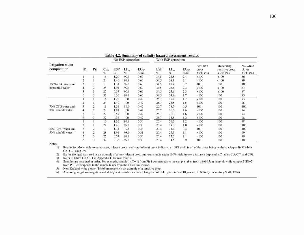
130
Table 4.2. Summary of salinity hazard assessment results. No ESP correction With ESP correction
Irrigation water composition ID Pit Clay ESP LFav ECSE ESP LFav ECSE
Sensitive crops
Moderately sensitive crops
NZ White clover
% % % dS/m % % dS/m Yield (%) Yield (%) Yield (%) 1 1 16 1.20 99.9 0.60 34.5 24.8 2.4 <100 <100 86 2 1 24 1.40 99.9 0.60 34.5 28.1 2.1 <100 <100 89 3 2 13 1.31 99.9 0.60 34.5 87.4 0.7 100 100 100 4 2 28 1.91 99.9 0.60 34.5 25.6 2.3 <100 <100 87 5 3 27 0.57 99.9 0.60 34.5 25.6 2.3 <100 <100 87
100% CSG water and no rainfall water
6 3 32 0.36 99.9 0.60 34.5 34.9 1.7 <100 100 93 1 1 16 1.20 100 0.42 26.7 25.4 1.7 <100 100 93 2 1 24 1.40 100 0.42 26.7 28.5 1.5 <100 100 95 3 2 13 1.31 89.0 0.47 26.7 78.7 0.5 100 100 100 4 2 28 1.91 100 0.42 26.7 26.3 1.6 <100 100 94 5 3 27 0.57 100 0.42 26.7 26.3 1.6 <100 100 94
70% CSG water and 30% rainfall water
6 3 32 0.36 100 0.42 26.7 34.5 1.2 <100 100 98 1 1 16 1.20 99.9 0.30 20.4 26.3 1.2 <100 100 98 2 1 24 1.40 99.9 0.30 20.4 29.3 1.0 <100 100 100 3 2 13 1.31 79.8 0.38 20.4 71.4 0.4 100 100 100 4 2 28 1.91 98.0 0.31 20.4 27.3 1.1 <100 100 99 5 3 27 0.57 99.9 0.30 20.4 27.3 1.1 <100 100 99
50% CSG water and 50% rainfall water
6 3 32 0.36 99.9 0.30 20.4 34.6 0.9 100 100 100 Notes:
1) Results for Moderately tolerant crops, tolerant crops, and very tolerant crops indicated a 100% yield in all of the cases being analysed (Appendix C tables C.5, C.7, and C.9).
2) Barley (forage) was used as an example of a very tolerant crop, but results indicated a 100% yield in every instance (Appendix C tables C.5, C.7, and C.9). 3) Refer to tables C.4-C.11 in Appendix C for raw results. 4) Samples are arranged in order. For example, sample 1 (ID=1) from Pit 1 corresponds to the sample taken from the 0-15cm interval, while sample 2 (ID=2)
from Pit 1 corresponds to the sample taken from the 15-45 cm section. 5) New Zealand white clover (Trifolium reperis) is an example of a sensitive crop 6) Assuming long-term irrigation and steady-state conditions these changes could take place in 5 to 10 years (US Salinity Laboratory Staff, 1954)

131
An example with an actual crop used for grazing in New Zealand (white clover or
Trifolium reperis) shows how the yield of a sensitive crop can become affected by CSG
water (Table 4.2). In this example, when using solely 100% CSG water, this crops’s yield
is often less than 90% especially in those soil samples with the largest clay percentage
(Table 4.2). However, if this water is blended with 30% rainfall water, the yield improves
so this time it is above 90%. If the CSG water is blended with 50% rainfall water, yield
improves significantly (above 98 %).
In addition, CSG water itself can be used to analyse the salinity hazard affecting
the water availability to crops just by analysing the specific conductance of the water.
Doing so can provide independent support to the results of applying the salinity model
(Table 4.2). In this case, Maramarua CSG water has a specific conductance of 1.31 dS/m
so this water is classified as having a “slight to moderate” restriction on its use for
irrigation (Ayers et al., 1985).
Discussion
The salinity model described in the preceding section shows how, with increasing
CSG discharge, soil salinity problems become evident. The model has to be used with
care because it has been developed mainly for arid and semi-arid conditions, and some of
its assumptions might not be relevant to New Zealand. For example, the relationship
linking soil ESP to SAR (Appendix C Eq. C.6) has been established for Western United
States soils which exist under completely different weather conditions than the ones for
New Zealand. Thus soil response to high-SAR water might not be as drastic as the one
depicted by this relationship, and long-term ESP values might be lower than anticipated
but no lower than the results obtained without ESP correction (Table 4.2). Also, salinity
effects will vary with depth and this would also have to be considered. For example, the
ANZECC guidelines state that changes in salinity could be noticed in a matter of months
for surface soils (1-10cm), while changes in ESP and CEC in deeper soil sections could
take up to several years to take effect (ANZECC and ARMCANZ, 2000). In any case,
this soil salinity model has shown how irrigation with CSG water can have an impact on
soil salinity and crop yield for sensitive and moderately sensitive crops.

132
Salinity in itself can improve the permeability of soils, and this can be observed
with the increase in leaching fraction when comparing solely rain-fed conditions against
the condition where soils are irrigated with CSG water (LFav values in Table 4.2).
However, when the soil ESP increases due to continuous CSG water irrigation, the
leaching fraction gets reduced. This is because some of the sodium will hydrolyze (due to
the presence of OH-) or tend to associate with bicarbonate ions (HCO3-) with decreasing
salinity (US Salinity Laboratory Staff, 1954); if the clay fraction is significant, the soil
will become dispersed by the sodium ions now in solution, and a loss in permeability will
have taken place. This was observed in Table 4.2 where samples with the higher clay
percentage (samples 1, 2, 4, 5, and 6) tended to experience the highest loss in leaching
fraction. This is more evident when the change in leaching fraction under rain-fed
conditions is compared against the leaching fraction under CSG water irrigation with and
without ESP correction (Appendix C, Table C.11). Thus, continuous CSG water
irrigation will increase soil ESP, and this in the long run will decrease the leaching
fraction. As less water is leached from the soil profile, more salts are retained after
evaporation, and the soil increases its overall salinity. This was observed in Table 4.2 as
the specific conductance of the soil (ECSE) increased as ESP values increased with
increasing CSG water irrigation.
For this particular location and CSG water quality, salinity appears not to pose a
serious risk. However, the FAO guidelines (Ayers et al., 1985) may indicate a more
significant hazard potential (slight to moderate). The boundary between “slight” and
“moderate” is not clear with these guidelines, and this might lead to an overestimation of
the effects of CSG water discharge.
Assessment of soil infiltration problems In the previous section, modelling results indicated that an increase in soil sodium
content (ESP) generates lower leaching fractions, which translates into a loss of
permeability. In this case, the decrease in leaching was not significant enough to cause
significant losses in yield. However, with higher clay contents and higher sodium
concentrations the problem could become aggravated. This problem is particularly
important right after rainfall because salts will be leached from the soil, but sodium will

133
be retained attached to clay particles. As a consequence, ESP value will be maintained
while soil salinity will decrease, and soil dispersion will take place (ANZECC and
ARMCANZ, 2000). Therefore it is necessary to assess the loss of structural stability
(infiltration loss) due to continuous CSG water discharge.
Figure 4.10, is a magnification of Figure 4.3 showing the risk of infiltration loss
associated with soils in the Maramarua (C-1) area. This figure shows that soils in the
vicinity of C-1 can have either a low, moderate, or high infiltration problem. The soils
towards the southwest of C-1 are at high risk because, according to the FSDL, these soils
are classified as clays, which puts them at high risk of dispersing when irrigated with
CSG water. However, soil samples collected from approximately 100 m south of C-1 had
a low clay content, and are classified as loams (Figure 4.9).
To evaluate potential infiltration problems, the ANZECC guidelines recommend
an assessment using the specific conductance (in logarithmic form) and SAR of irrigation
waters (ANZECC and ARMCANZ, 2000). The FAO guidelines recommend a similar
procedure, but with specific conductance in linear form while applying a calcium
carbonate precipitation correction to the calculated SAR values. These guidelines assume
well-drained loams (sand loams to clay loams) in semi-arid or arid climates, so they have
to be used carefully in humid climates. Nevertheless, it is still possible to use them in
humid climates in conjunction with other analyses (like the calculation of leaching
fractions and IPP index). A plot showing the SAR values vs. the logarithm of the specific
conductance (EC) for Maramarua CSG water, according to the ANZECC guidelines, is
presented in Figure 4.11 (a similar graph showing the same results but using the FAO
guidelines is presented in Figure C.4, Appendix C). In addition to presenting pure CSG
water, different combinations resulting from blending CSG water with rain water and
wetland water (adjacent Kopuku swamp) are shown in the same figure. Rain water is
assumed to have a specific conductance value of 0.03 dS/m, whereas wetland water is
assumed to have a specific conductance value of 0.273 dS/m (measured on site). Both
blending waters are assumed to have nil sodium concentrations, and results from these
blendings have not been corrected for calcium carbonate precipitation, so actual SAR
values could be higher than the ones shown in the graph.
134
Figure 4.11 shows that irrigation with pure CSG water will produce soil
infiltration problems (loss of water and air permeability), and no blending combination
will be able to correct this problem. Even blendings with higher rain-water or wetland-
water volumes will produce a water quality within the hazardous zone; blending with
90% wetland water almost reduces the problem to acceptable levels, but this water
blending is highly inefficient as a method of CSG water disposal (only 10% reduction).
Soils in Maramarua could experience soil infiltration problems if exposed to CSG
water. An initial look at the distribution of the IPP index in the area (Figure 4.10) shows
that there are some soils in the vicinity of C-1 with a high potential for infiltration
reduction if exposed to high-SAR water. This was verified by calculating the leaching
fraction and soil salinity resulting from Maramarua CSG water disposal on these soils
over a prolongued period of time (5-10 years according to USSL, 1954). Results
indicated a significant reduction in leaching fraction, which would result in an important
loss in soil permeability. This is verified by the SAR/Salinity diagram in
Figure 4.11, which indicates that soils’ structural problems are likely to occur if CSG
water is disposed on these soils.

135
Figure 4.10. Infiltration problem potential at Maramarua due to high-SAR water discharges

136
0.1 0.2 1 2 100
5
10
15
20
25
30
36.5
1.3
EC (dS/m)
SA
R⊗
Soil
stru
ctur
al
prob
lem
s ar
e lik
ely
Stab
le s
oil
stru
ctur
e
Dep
ends
on
soil
prop
ertie
san
d ra
infa
ll
�
�
�
�
��
�
Figure 4.11. Assessment of soil degradation using SAR and EC of irrigation water. Adapted from ANZECC (2000).

137
Assessment of specific ion toxicity
When applying the FAO toxicity guidelines presented in Table 4.1, the effects of
irrigating with Maramarua CSG water range from “slight” to “severe”. For example, the
SAR of CSG water from C-1 is 36.5, and the lower limit for the “severe” restriction
category (to assess sodium toxicity) in the FAO guidelines is 9. Similarly, chloride and
boron concentrations produce effects which range from “slight” to “moderate”.
The ANZECC guidelines provide a description of the crops that can be grown
under specific ion concentrations. Under these guidelines, the use of Maramarua CSG
water for irrigation does not generate any restrictions in relation to chloride, but its
sodium concentrations may pose a problem for “sensitive”, “moderately sensitive”, and
some “moderately tolerant” crops (Table 4.3). In addition, the high-SAR of this CSG
water (36.5) can generate leaf scorch and leaf tip burn in crops like avocado, deciduous
fruits, nuts, and citrus, and it can have a stunted growth effect in beans. These effects
along with sodium toxicity and possible calcium or magnesium deficiency may also
extend to crops like clover, oats, tall fescue, rice, and dallis grass (ANZECC and
ARMCANZ, 2000). Boron concentrations may also pose a problem when irrigating with
CSG water from Maramarua. In this case, short-term effects could be noticed in very
sensitive crops (blackberry and lemon), sensitive crops (onion, garlic, sweet potato, wheat,
and barley), moderately sensitive crops, (pea, carrot, and potato), and in some moderately
tolerant crops (lettuce, clover, oat, and corn) (Ayers et al., 1985, as cited in ANZECC and
ARMCANZ 2000).

138
Table 4.3. Crop tolerance to sodium and chloride toxicity associated with Maramarua CSG water Ion CSG Water
mg/l Sensitive Moderately
sensitive Moderately tolerant
Tolerant
Chloride 146 OK OK OK OK Sodium 334 Not OK Not OK May be OK OK Notes: CSG water from Maramarua C-1 (19/8/2004 sample, see Chapter 2) Sensitive crops: almond, apricot, citrus, plum, grape Moderately sensitive: pepper, potato, tomato Moderately tolerant: barley, maize, cucumber, lucerne, safflower, sesame, sorghum Tolerant: cauliflower, cotton, sugar beet, sunflower
Blending CSG water with rain water or surface water could lower the
concentration of specific ions like sodium or boron so that guidelines limits are met.
However, the water used for blending needs to have a significantly lower concentration
value for the specific ion under consideration. For example, a blending of 50% CSG
water and 50% rain water would generate a final sodium concentration of 168 mg/l which
would enable irrigation on “moderately tolerant crops” and on some “moderately
sensitive crops”. Using more rain water (70%) and less CSG water (30%) would yield a
final concentration of 101mg/l which would clear any sodium toxicity problems (even in
sensitive crops), however this method does not allow the disposal of large amounts of
CSG water. In addition, blending would require large ponds and mixing equipment,
which would increase costs and project footprint.

139
Effects arising from surface water disposal of CSG waters
The Maramarua basin under exploration is administered by Environment Waikato.
This council has a regional policy statement which will be implemented by a proposed
regional plan. At the time of the writing of this thesis, the Waikato Regional Plan was
being revised by the Environment Court. However, it is foreseen that the final plan will
not include major changes, so the policies and methods included in the Proposed Waikato
Regional Plan (PWRP), can be used to assess the effects of disposing CSG waters on
surface waters in the Maramarua area. In addition, the methodology outlined in the plan
can be complemented by using the ANZECC water quality guidelines.
Because full-scale production is not yet underway in Maramarua, the total amount
of water to be disposed of is unknown. This value will depend on the number of
production wells and the rate at which these will be producing CSG water. For example,
if 20 wells are drilled in this basin, and each well produces 40m3 of CSG water per day,
then the total amount to be disposed of will be 800m3/day. This quantity of water would
have an impact on low lying areas around the region. For example, the Whangamarino
wetland has a “wet/dry” seasonal cycle (Department of Conservation, 2006b), and its
water level rarely surpasses the 5 metre mark (Environment Waikato, 2006).
Under the discharge-to-water scenario, analytes of concern would have to be
monitored only after reasonable mixing of CSG water with the receiving surface water
body (Environment Waikato, 2002). Different standards would apply depending on the
use of the water body, and monitoring would have to be enforced. For example, specific
ions or properties to monitor would be changes in pH, dissolved oxygen, and temperature.
The ANZECC guidelines recommend a trigger value of 7.8 for pH values in
lowland river areas. The nearest stream to C-1 is Kopuku stream, which flows through
Kopuku Wetland. Since this stream is located in a lowland area, the 7.8 pH trigger value
would apply. Maramarua CSG water has an initial pH of 7.4 once pumped to the surface;
however, as this water reaches equilibrium with the atmosphere, its pH can rise up to 8.6
(see chapter 2), therefore monitoring of pH values after mixing would have to be carried
out. Dissolved oxygen readings were carried out on-site with a meter in September 2004.
The minimum DO saturation (%) reading detected at the wellhead was 22.5%, but this

140
value is significantly higher than the one for Kopuku Wetland (3.9%). In addition, the
temperature at the wellhead was 18.3°C which is 5.6°C higher than the temperature
measured on that same day for the wetland (12.7°C). The PWRP states that, as a result of
permitted activities, the water temperature of the receiving body must not change in more
than 3°C, so temperature would also have to be monitored. Since the PWRP states that
permitted discharges into surface water bodies must not make the surface water
unsuitable for irrigation, specific ions and properties like sodium, chloride, boron, and
salinity would also have to be monitored.
It is unlikely that a resource consent to discharge Maramarua CSG water into the
Kopuku and Whangamarino wetlands would be granted because the Whangamarino
wetland is listed under the 1996 Waikato Conservancy Conservation Management
Strategy as an area requiring protection (Environment Waikato, 2002). The Kopuku
Wetland and stream are connected to Whangamarino wetland, and any discharge would
affect the latter. However, it is important to study the effects of potential CSG water
discharge into the Kopuku Wetland because, if land disposal is implemented, CSG water
disposed on the land could find its way to this wetland (or Whangamarino) in the form of
surface runoff or subsurface flow.
Potential effects on aquatic life
The freshwater fish database (managed by NIWA) has data on the different
species of fish in the Kopuku area between 1983 and 1988. The species of native fish
recorded were Black mudfish (Neochanna diversus), Koaroa (Galaxias brevipinnis),
Longfin eel (Anguilla dieffenbachii), Crans bully (Gobiomorphus basalis), Common
bully (Gobiomorphus cotidianus), Shortfin eel (Anguilla australis), and Banded kokopu
(Galaxias fasciatus); while the exotic fish registered at the site were Goldfish (Carassius
Auratus), Catfish (Ameiurus nebulosus), and Gambusia (Gambusia affinis) (NIWA,
2006b).
From the list, two native species of interest are Banded kokopu and Shortfin eels
because, as previously mentioned, these species are noted for preferring less-than-neutral
pH values; since the pH measured at Kopuku is 6.59, these fishes can live in this
environment. However, if Kopuku Wetland starts receiving CSG water, its pH could

141
increase above neutral levels. As a result, Shortfin eels and Banded kokopu could end up
abandoning these wetland areas to live in environments with lower pH values.
Gambusia is an introduced species in New Zealand and is considered undesirable
for their extremely aggressive nature and propensity to attack native fish (NIWA, 2006b).
In particular, Gambusia are known to attack young Black mudfish, which is listed as
“indeterminate” in the threatened species list (LFTB Study Group., 1986). However
Black mudfish are able to co-exist with Gambusia because of their ability to survive in
environments that dry up periodically, whereas Gambusia do not (NIWA, 2006b). This is
significant in the Whangamarino wetland, as this area has a hydrological regime
exhibiting a “wet/dry” seasonal cycle (Department of Conservation, 2006b). CSG water
discharges could alter this equilibrium by supplying extra quantities of water to zones that
normally would dry up. This could put Black mudfish at the mercy of Gambusia, and
their numbers could decrease.
Increasing salinity, as a result of CSG water discharges, could also endanger some
species. Most of the native species listed are diadromous and would be able to survive in
saline environments. However, Crans bullies do not have a marine phase and are non-
diadromous (NIWA, 2006b); their ability to survive in a wetland receiving CSG water
discharge would be limited.
Potential effects on vegetation
The vegetation found near C-1 corresponds to the vegetation of Kopuku and
Whangamarino wetlands. These consists of sedges (Baumea), Manuka (Leptospermum
scoparium), and Wire rush (Empodisma minus). In addition, various threatened plants
have been registered in the wetland including Club moss (Lycopodium serpentinum),
Orchid (Corybas carseii), and Water milfoil (Myriophyllum robustum) (Department of
Conservation, 2006b). In addition, marginal vegetation like Carex secta, Coprosma
tenuicaulis, Juncus, Flax, and Cabbage trees along with Kahikatea (Podocarpus
dacrydiodes) and Climbing fuchsia (Fuchsia perscandens) can be found at the northern
end of Kopuku Wetland (LFTB Study Group., 1986). Also, most of the Whangamarino
wetland is covered with introduced willows (Salix cinerea and S. fragilia).
142
CSG water discharges into these wetland areas could generate negative impacts
on native vegetation from increased water levels and salinity. For example, studies
carried out by Eser (2000) suggested that increasing Lake Taupo’s water levels would
most likely decrease native plant communities, while promoting the spread of Salix
cinerea in the Stump Bay wetland (adjacent to Lake Taupo). The same effect could take
place in the Whangamarino and Kopuku wetlands if CSG water discharges produce a
significant increase in water levels. In addition, the salinity of CSG waters could alter the
salinity of the receiving wetlands negatively affecting plant communities. Sedges, for
example, have very low tolerance to salinity (<0.5 ppt) (Knight, 1997) so their ability to
grow would become impaired as salinity increases due to CSG discharges (C-1 salinity =
0.65 ppt).
These effects are unlikely to be detected at once, however as more wells are
completed and these wetlands receive CSG water, effects would start to take place
depending on the quantity and quality of the water being discharged. In particular, effects
would be most noticeable at margins and in zones experiencing natural dry periods. Once
more information becomes available, it will be important to carry out mixing and dilution
studies to determine the extent of these effects.

143
Conclusions
The effects arising from CSG water disposal are tangible, and can be identified
according to the selected method of disposal. If CSG waters are disposed on land, this
could result in increased soil salinity, degradation of soil structure, and plant toxicity
effects. On the other hand, if CSG waters are disposed on surface waters, the potential
effects include the loss of riparian vegetation and fish communities. Sometimes, this loss
can have significant implications on biodiversity as resilient species flourish while more
sensitive species disappear. Also, the extent of these effects depends on the specific
conditions at each basin where CSG water is being disposed.
The effects of CSG water disposal clearly depend on the ultimate fate of CSG
water. Some methods of disposal could produce significant effects (surface water
disposal to small streams or wetlands for example), while others would generate
negligible effects (i.e. aquifer injection). However, if there are links between receiving
environments the problem becomes complicated. For example, if CSG waters are
disposed on a river, its aquatic fish and plant communities become affected, but if water
is abstracted for irrigation downstream from the discharge point, the effects could extend
to crops on the receiving soils.
When CSG waters are disposed on land, its dissolved ions (mainly sodium,
bicarbonate, and chloride) become part of the soil-water solution and tend to remain
within the soil structure. Soil salinity will promote permeability by keeping particles
flocculated, and this has been observed by Oster and Schroer (1979) and US Salinity
Laboratory Staff (1954) among others. Although increased soil salinity does not damage
soils, it has negative effects on plants as these need to exert an extra effort in extracting
water from the soil-water solution. During rainfall events most of these ions are leached
from the soil thus reducing soil salinity levels. However, sodium cannot be removed by
this method because this ion remains adsorbed to the soil clay particles. In this chapter,
the same effects were noted when analysing data from Maramarua. In this case, CSG
water discharges would cause an increase in ESP values, which in turn would increase
soil salinity values. Long term salinity effects for this location would impair these soils
for the cultivation of sensitive crops and moderately sensitive crops. Likewise, the FAO
144
water quality irrigation guidelines recommend care when irrigating with water quality
like the one for Maramarua CSG water.
The more clay particles a soil has, the more sodium will remain adsorbed to its
clay component. Once a soil starts to accumulate sodium, it becomes prone to dispersion.
That is, its clay particles will become attracted to each other (due to the sodium ion) and
will become rearranged. This will cause loss of aggregation which results in overall loss
of permeability. This problem has been observed with high-SAR irrigation water by US
Salinity Laboratory Staff (1954), Ayers and Westcot (1985), and Oster and Schroer
(1979). Most recently Robinson (2003) verified these effects experimentally using CSG
water and soils from the PRB. Maramarua CSG water could generate the same infiltration
problems with soils from the area. Various CSG water and freshwater blendings would
generate water solutions having SAR/salinity combinations which could produce soil
infiltration problems in the long-run. These problems are mainly due to the high-SAR
content of CSG waters from Maramarua, and the moderate clay content in some of the
soils in the area.
The SAR component of CSG waters can easily be underestimated. This is because
CSG waters have a high bicarbonate content and are generated in underground
environments exposed to high hydrostatic pressures. However, once these waters are
pumped to the surface they become exposed to normal atmospheric pressure, and calcium
is precipitated in the form of calcium carbonate. This effect was measured experimentally
in Chapter 3, and it was responsible for a 23% increase of the original SAR values. In this
chapter, this effect was taken into account by correcting CSG water quality from
Maramarua (19/8/2004) using the procedure described by Suarez (1981). As a result,
SAR values increased from 33.6 to 36.5 (8.6%). Therefore, SAR values from CSG water
samples need to be adjusted to account for calcium carbonate precipitation. The
procedure proposed by Suarez (1981) is an effective approximation, but an exact value
can be calculated if sparging experiments (like the one carried out in Chapter 3) are
carried out.
Other effects associated with CSG water discharge, which have been noted in the
Maramarua case study include specific toxicity issues related to some of its ions. In
particular, sodium and boron toxicity problems could become a problem in sensitive

145
crops. The effects of sodium could extend even to moderately tolerant crops, but its
effects could be mitigated if CSG waters are blended with waters having low sodium
concentrations. In addition, chloride concentrations could pose “slight” to “moderate”
effects depending on the type of crop being grown.
Effects of CSG water discharges into surface waters are more difficult to quantify
because these depend on the nature of plant and fish communities present in the receiving
bodies. In the US, effects have been noted in riparian vegetation of the PRB and some
fish communities in the Black Warrior Basin. In Maramarua, the effects have not been
noticed at this stage because full-scale water production has not yet begun. However,
native fish species like Banded kokopu and Shortfin eels could become affected by an
increase in pH due to CSG water discharges. In addition, other native fishes could end up
being displaced by introduced species (like Gambusia) if CSG waters improve the
habitats of the introduced species. However, most native New Zealand fishes spend some
time living in the sea, so they would have some ability to adapt to increased salinity and
pH arising from CSG water discharges. Riparian plant communities would be affected in
a similar way as the vegetation growing on soils exposed to CSG water discharges. These
plants would mainly be exposed to high ion toxicity resulting from sodium, chloride, and
boron. In this way, sensitive species could disappear while more resilient species could
invade areas formerly inhabited by these sensitive species. For example, in the Kopuku
and Whangamarino wetlands the noxious Salix cinerea could end up spreading as a result
of CSG discharges, while more sensitive native species like Sedges could end up
disappearing.
In this chapter, the effects associated with CSG water discharges have been
studied using background literature studies supported by a case study of the Maramarua
area. This case study has provided an assessment based on the ANZECC water quality
guidelines (2000). Throughout this chapter, a new methodology for assessing potential
environmental effects associated with CSG water management has been developed using
pre-existing concepts and environmental guidelines. This includes assessment of CSG
water quality, soils, surface waters, plant and aquatic life in relation to disposal
operations. Much of the analysis in this chapter is based on conjecture because of the
current lack of data; still, it is hoped that this work will help future investigators by

146
identifiying key issues and appropriate approaches to environmental impact assessment.
Similar studies to this one could be carried out for other CSG sites around New Zealand
once CSG water quality data for these sites becomes available. While some regions (i.e.
Ashers-Waituna) are located in areas of low risk, other regions like Hawkdun would be
prone to problems arising from CSG water disposal. For purposes of issuing resource
consents, similar analyses like the one performed on Maramarua could be carried out on
each site where CSG development will take place.
147
References
ALL-Consulting, 2003, Handbook on Coal Bed Methane Produced Water: Management
and Beneficial Use Alternatives.: Tulsa, Oklahoma, Ground Water Protection
Research Foundation, US Department of Energy, National Petroleum Technology
Office, Bureau of Land Management.
ALL-Consulting, and Montana Board of Oil and Gas Conservation, 2004, Coal Bed
Methane primer. New Source of Natural Gas–Environmental Implications.
Background and Development in the Rocky Mountain West: Tulsa, Oklahoma,
US Department of Energy, National Petroleum Technology Office.
Allen, R.B., McIntosh, P.D., and Wilson, J.B., 1998, The distribution of plants in relation
to pH and salinity on inland saline/alkaline soils in Central Otago, New Zealand.
(vol 35, pg 517, 1997): New Zealand Journal of Botany, v. 36, p. 153-153.
ANZECC, and ARMCANZ, 2000, Australian and New Zealand Guidelines for Fresh and
Marine Water Quality, ACT: Australian and New Zealand Environmental and
Conservation Council (ANZECC), Agricultural and Resource Management
Council of Australia and New Zealand (ARMCANZ): Canberra.
Ayers, R.S., Westcot, D.W., and Food and Agriculture Organization of the United
Nations., 1985, Water quality for agriculture: Rome, Food and Agriculture
Organization of the United Nations, xii, 174 p.
Bauder, J., 2001, Quality and Characteristics of Saline and Sodic Water Affect Irrigation
Suitability: MSU, Bozeman, MT, p. http://waterquality.montana.edu.
Bodger, F., 2005, The use of coal seam gas waters in New Zealand to treat acid mine
drainage, Civil Engineering: Christchurch, University of Canterbury, p. 44.
Bresler, E., McLean, B.L., and Carter, D.L., 1982, Saline and sodic soils: Principles-
dynamics-modeling., Advanced series in agricultural sciences., Volume 10: New
York, NY, Springer-Verlag.
Burkett, W.C., McDaniel, R., and Hall, W.L., 1991, The Evaluation and Implementation
of a Comprehensive Production Water Management Plan, Coalbed Methane
Symposium: Tuscaloosa, Alabama.

148
Cameron, K.C., Di, H.J., Anwar, M.R., Russell, J.M., and Barnett, J.W., 2003, The
"critical" ESP value: does it change with land application of dairy factory
effluent?: New Zealand Journal of Agricultural Research, v. 46, p. 147-154.
Cavanagh, J., and Coakley, J., 2005, An introduction to policy on metal contaminants, in
Moore, T.A., Black, A., Centeno, J.A., Harding, J.S., and Trumm, D.A., eds.,
Metal Contaminants in New Zealand, Volume In Press, Corrected Proof:
Christchurch, resolutionz press, p. 5-23.
Collier, K.J., Ball, O.J., Graesser, A.K., Main, M.R., and Winterbourn, M.J., 1990, Do
organic and anthropogenic acidity have similar effects on aquatic fauna?: Oikos, v.
59, p. 33-38.
Davis, H.A., Simpson, T.E., Lawrence, A.W., Miller, J.A., and Anonymous, 1993,
Coalbed methane produced water management strategies in the Black Warrior
Basin of Alabama: Proceedings - International Coalbed Methane Symposium, v.
1993, p. 317-338.
Davis, W.N., Bramblett, R.G., and Zale, A.V., 2006a, Effects of coalbed natural gas
activities on fish assemblages in the Powder River Basin, 2005, in Montana
Cooperative Fishery Research Unit, ed.: Bozeman, Montana State University, p. 3.
—, 2006b, The effects of coalbed natural gas activities on fish assemblages: a review of
the literature: Bozeman, Montana State University, p. 48.
Department of Conservation, 2006a, New Zealand map service, DOCgis GeoSpatial
Information Platform, p. http://extranet.doc.govt.nz/bip/.
—, 2006b, New Zealand's Wetlands of International Significance: Whangamarino,
http://www.doc.govt.nz/Conservation/Wetlands/.
Detmer, E., 2005, Zeolite water conditioning system: Sheridan, p. Personal conversation.
Environment Waikato, 2002, Waikato Regional Plan - Proposed plan and maps on CD-
ROM as amended by decisions (appeals version), in Waikato Regional Council,
ed.: Hamilton, Waikato Regional Council,.
—, 2006, River Levels and Rainfall. Whangamarino Wetland. Levels at Ropeway on
Island Block Road, Meremere, Volume 2006: Hamilton, Environment Waikato, p.
web page and online database system.
149
Eser, P., and Rosen, M.R., 2000, Effects of artificially controlling levels of Lake Taupo,
North Island, New Zealand, on the Stump Bay wetland: New Zealand Journal of
Marine and Freshwater Research, v. 34, p. 217-230.
Jensen, M.E., 1983, Design and operation of farm irrigation systems: St. Joseph, Mich.,
American Society of Agricultural Engineers, xi, 829 p. p.
Kirkpatrick, A.D., 2005, Assessing constructed wetlands for beneficial use of saline-sodic
water: Bozeman, Montana State University,.
Knight, R.L., 1997, Wildlife habitat and public use benefits of treatment wetlands: Water
Science and Technology, v. 35, p. 35-43.
Kristin, K., Bauder, J., and Wheaton, J.R., 2006,
http://waterquality.montana.edu/docs/methane/cbmfaq.shtml, Water quality and
Irrigation Management, Volume 2006: Bozeman, Montana State University.
Landcare Research New Zealand Ltd, 2000a, New Zealand Land Resource Inventory
(NZLRI): Lincoln, Landcare Research New Zealand Ltd.
—, 2000b, The New Zealand National Soils Database Spatial Extension, Soil
Fundamental Data Layers: Lincoln, Landcare Research New Zealand Ltd.
Lee-Ryan, P.B., Fillo, J.P., Tallon, J.T., and Evans, J.M., 1991, Evaluation of
management options for coalbed methane produced water, Coalbed methane
symposium: Tuscaloosa, Alabama, The University of Alabama,, p. 31-41.
LFTB Study Group., 1986, South Island Phase II Lignite Site Selection Studies
Programme. Resource definition, geotechnical, hydrology, and mine planning
studies. Hawkdun deposit.: Wellington, N.Z., Liquid Fuels Trust Board.
Main, M.R., 1988, Factors influencing the distribution of kokopu and koaro (Pisces:
Galaxiidae) : a thesis submitted in partial fulfilment of the requirements for the
degree of Master of Science in Zoology in the University of Canterbury, 127
leaves, [36] leaves of plates p.
McBeth, I., Reddy, K.J., and Skinner, Q.D., 2003, Chemistry of trace elements in coalbed
methane product water: Water Research, v. 37, p. 884-890.
McIntosh, A., and McDowall, R., 2004, Fish Communities in rivers and streams, in
Harding, J.S., New Zealand Hydrological Society., and New Zealand
Limnological Society., eds., Freshwaters of New Zealand: [Wellington, N.Z.],

150
New Zealand Hydrological Society ; New Zealand Limnological Society, p. 17.1-
17.9.
McLaren, R.G., and Cameron, K.C., 1990, Soil science : an introduction to the properties
and management of New Zealand soils: Auckland, N.Z., Oxford University Press,
viii, 294 , 8 of plates p.
Menneer, J.C., McLay, C.D.A., and Lee, R., 2001, Effects of sodium-contaminated
wastewater on soil permeability of two New Zealand soils: Australian Journal of
Soil Research, v. 39, p. 877-891.
Montana State University, 2006a, Coal Bed Methane Water Treatment System,
http://waterquality.montana.edu/docs/methane/cbm-wts.shtml, Montana State
University., p. Drake Engineering Inc. Water Treatment System.
—, 2006b, Frequently Asked Questions Coal Bed Methane (CBM), Volume 2006:
Bozeman, Montana State University, p. Web page
http://waterquality.montana.edu/docs/methane/cbmfaq.shtml.
New Zealand. Mines Division., Longworth McKenzie Cole., and Worley Consultants
Ltd., 1983, New Zealand coal resources survey : preliminary mining and
environmental constraints assessment pilot study : Maramarua coalfield:
[Wellington, N.Z.], Mines Division Ministry of Energy, 2 v. p.
NIWA, 2006a, NIWA Atlas of New Zealand Freshwater Fishes, Common smelt
(Retropinna retropinna),
http://www.niwascience.co.nz/rc/freshwater/fishatlas/species/common_smelt,
Volume 2006, NIWA.
—, 2006b, NZFFD, New Zealand Freshwater Fish Database, NIWA, p.
http://www.niwascience.co.nz/services/nzffd/.
O'Neil, P.E., Harris, S.C., and Mettee, M.F., 1989, Stream Monitoring of Coalbed
Methane Produced Water from the Cedar Cove Degasification Field, Alabama,
The 1989 Coalbed Methane Symposium: Tuscaloosa, Alabama, The University of
Alabama,.
Oster, J.D., and Schroer, F.W., 1979, Infiltration as Influenced by Irrigation Water-
Quality: Soil Science Society of America Journal, v. 43, p. 444-447.
151
Pope, S., and Trumm, D., 2004, Coal Seam Gas Desorption Results: Drill Holes C1, K1 and K3,
Maramarua Coalfield, Waikato, 2003.: Christchurch, CRL Energy Ltd, p. 27.
Rice, D.D., 1993, Composition and origin of coalbed gas, in Law, B.E., and Rice, D.D., eds.,
Hydrocarbons from coal, Volume AAPG Studies in Geology, American Association of
Petroleum Geologists, p. 159-184.
Robinson, K.M., 2003, Effects of saline-sodic water on EC, SAR, and water retention:
Bozeman, Montana State University.
Scarsbrook, M.R., and National Institute of Water and Atmospheric Research (N.Z.),
2003, A guide to the groundwater invertebrates of New Zealand: Wellington
[N.Z.], Niwa, 59 p.
Settle, T., Mollock, G.N., Hinchman, R.R., and Negri, M.C., 1998, Engineering the use of
green plants to reduce produced water disposal volume., Society of Petroleum
Engineers: Inc. Devon Energy Corporation, Oklahoma City, OK. Argonne
National Laboratory, Argonne IL.
Shainberg, I., and Letey, J., 1984, Response of Soils to Sodic and Saline Conditions: Hilgardia, v.
52, p. 1-57.
Suarez, D.L., 1981, Relationship between pHc and sodium adsorption ratio (SAR) and an
alternative method of estimating SAR of soil or drainage waters: Soil Science Society
of America Journal, v. 45, p. 469-475.
Taulis, M., Milke, M., Trumm, D., O'Sullivan, A., Nobes, D., and Manhire, D., 2005,
Characterisation of Coal Seam Gas waters in New Zealand, 2005 New Zealand
Minerals Conference: Auckland, New Zealand.
US Salinity Laboratory Staff, 1954, Diagnosis and improvement of saline and alkali soils:
[Washington,, US Govt. Print. Off.], vii, 160 p. p.
Van Voast, W.A., 2003, Geochemical signature of formation waters associated with coalbed
methane: Aapg Bulletin, v. 87, p. 667-676.
West, D.W., Boubée, J.A.T., and Barrier, R.F.G., 1997, Responses to pH of nine fishes and one
shrimp native to New Zealand freshwaters: New Zealand Journal of Marine and
Freshwater Research, v. 31, p. 461-468.
Wheaton, J.R., and Donato, T.A., 2004, COALBED-METHANE BASICS: Powder River Basin,
Montana: Butte, Montana Bureau of Mines and Geology, p. 20.
152
5. Chapter 5
Sodium removal from Maramarua coal seam gas waters using Ngakuru zeolites
Introduction
Zeolites are minerals having a porous structure, crystalline characteristics, and an
alumino-silicate configuration resulting in an overall negative charge which is balanced
by loosely held cations like Na+, K+, Ca2+, and Mg2+ (Christie et al., 2002). This makes
zeolites excellent materials to be used in cation exchange applications. In addition,
zeolites can also function as ionic sieves capable of absorbing certain ions and not others,
depending on the size of the cavities forming the porous structure and on the size of the
ions entering the zeolite structure (Coombs, 1959). Other properties of importance
include a high degree of hydration/dehydration, low density, good crystal stability when
dehydrated, and their ability to adsorb ions in gaseous form (Christie et al., 2002).
Common zeolite applications include their use as pet litter, oil/chemical and odour
absorbents, wastewater treatment, and their use as slow release fertilisers (NZ Natural
Zeolite, 2006).
Zeolites in New Zealand occur mainly in the Taupo Volcanic Zone, Northland ,
Auckland, and Southland (Christie et al., 2002). Ngakuru zeolites are located in the
Taupo Volcanic Zone about 20 km south of Rotorua. These zeolites are hydrothermally
altered and occur in lake sediment beds of Quaternary age up to 45 m deep (Mowatt,
2000). The main type of zeolites in Ngakuru is mordenite (40-80%) followed by
clinoptilolite (20-60%), and cristobalite (0-10%) (Mowatt, 2000). Bolan and Mowatt
(2000) have successfully used these zeolites in trials to remove ammonium cations in
wastewaters from tannery operations. In these experiments, wastewaters with ammonium
concentrations of 300 mg/l and 720 mg/l, were passed through columns containing 100 g
of zeolites at a flow rate ranging from 2.5 to 4.5 ml/min/kg zeolite. The zeolites were
capable of removing up to 77% of the ammonium cations in the wastewater. Previous

153
New Zealand studies by Nguyen and Tanner (1998) also focused on removing
ammonium cations but this time from dairy farm effluent and piggeries, and by using
clinoptilolite and mordenite obtained from different sites. Their studies concluded that the
ammonium removal capacity of these zeolites decreased when sodium ions were present
in the waste stream. This generated ammonium removal capacities of up to 15 % with the
mordenite, and 30% with the clinoptilolite.
Coal seam gas (CSG) waters are a new type of wastewater which could become
fairly common on the New Zealand landscape and waterways. These groundwaters are a
by-product of natural gas extraction from underground coal seams. Their production rate
sometimes can be as high as 40m3/day per well with as many as 13000 wells in areas like
the Powder River Basin, in the United States (Nelson, 2005). CSG waters tend to exhibit
similar quality in terms of salinity and major ion composition. Their specific conductance
varies depending on their travel time within the coal aquifer which accounts for different
degrees of mineralization, and their major ions are sodium, bicarbonate, and sometimes
chloride. Overall, these waters tend to be fairly alkaline with low calcium, magnesium,
and sulphate concentrations (Van Voast, 2003). The main issue with these waters is their
elevated sodium content, which in conjunction with their low calcium and magnesium
concentrations, can generate soil infiltration problems in the long run, as well as short
term toxicity effects in plants due to the sodium ion itself (see Chapter 4). Other toxicity
effects can arise due to their chloride content and to small amounts of boron (if present).
Coal seam gas is still under exploration in New Zealand, but its development is
imminent within the next few years. CSG water samples taken from CSG pilot scale
operations have produced CSG waters with high sodium and low calcium and magnesium
concentrations (Taulis et al., 2005), and their extraction rate has been as high as those
rates experienced in US basins. In New Zealand, the disposal of CSG waters is regulated
by Regional Councils, which promote land disposal of wastewaters over surface water
disposal (ANZECC and ARMCANZ, 2000). However, the environmental effects due to
CSG water disposal could extend to receiving environments both on the land and on
surface waters. In some instances, CSG waters could damage valuable agricultural soils
or riperian vegetation on protected ecosystems so restrictions on their disposal will be
stringent. On the other hand, CSG water quality could be good enough to ensure little or

154
no environmental damage, or the receiving environment could have a good capacity for
assimilating CSG water discharges. Therefore, treatment of CSG waters prior to disposal
will need careful consideration in many NZ CSG locations. One way of reducing sodium
concentrations of CSG waters might be by using New Zealand natural zeolites as
exchange materials. Treating CSG waters in this way could not only make CSG waters
comply with local regulations, but it could also transform CSG waters into a useable
water resource. There is a direct economic benefit from using Ngakuru zeolites instead of
commercial ion exchange resins. Ngakuru zeolites are easy to mine and readily available
– their price ranges from about NZ $75/tonne to $350/tonne depending on their quality
whereas the price of synthetic zeolites can be as high as NZ $ 69/kg (Christie et al., 2002).
Hence, the objective of this research is to study the feasibility of New Zealand natural
zeolites for CSG water treatment.
Materials and Methods
Materials
Ngakuru zeolite samples were obtained from NZ Natural Zeolite, a subsidiary of
Resource Refineries Ltd. Samples were provided in three sets; all of these were from a
quarry containing zeolites having a high cation exchange capacity (CEC) and good
resistance to mechanical breakdown. An additional zeolite sample (marketed as kitty
litter) with a lower CEC was obtained for comparison purposes when carrying out batch
experiments. These samples were sieved and grouped into 0.15-0.3 mm, 0.3-0.6mm, and
0.6-1.180mm particle size ranges. The moisture content for these samples ranged
between 3.4% and 4.5% with a specific density of about 1.5 g/cm3. X-ray diffraction
analyses were carried out on the high CEC samples at the Geological Sciences
Department (University of Canterbury) using an X-ray diffractometer for mineral
identification (see Appendix E). These analyses revealed that the main crystalline
materials present in these zeolites were 70-75% mordenite ( [Ca, Na2, K2] Al2Si10O24 –
7H2O, hydrated calcium sodium potassium) and 25-30% sanidine (KAlSi3O8, Potassium
Aluminum Silicate). Previous studies by Mowatt (2000) had revealed that their CEC
ranged from 40 to 110 meq/100 g, while their surface area ranged from 34 to 138 m2/g.

155
Synthetic solutions of NaCl, NaOH, HCl, CaCl2, and KCl in various
concentrations (ranging from 0.01M to 1 M ) were prepared for batch testing and
preliminary flow-through testing. These solutions were characterised by measuring their
pH and specific conductance according to APHA (1999) methods. For the final flow-
through study, actual Maramarua CSG water samples were used to assess the sodium
removal capacity of Ngakuru zeolites. These samples had been collected between August
and October, 2004, and April and June, 2005. The sample volumes remaining after
carrying out chemical analyses, had been stored at a temperature below 4°C. The samples
were combined and then filtered through a 1.2 µm glass filter, making up about 4.5 litres
of CSG water. The chemical analyses results for this composite sample are presented in
Table 5.1.

156
Table 5.1. Chemical analyses results for composite CSG samples Unit Composite sample
analysis 23/03/2006 CSG sample 19/08/2004
pH pH units 8.57 (1) 7.8 (4) Specific conductance µS/cm 1264 (1) 1310 (2) Total alkalinity mg/l as CaCO3 488 (2) 360 (4) SAR 29.6 33.6 Bicarbonate mg/l 564 (3) 435 (3) Sodium mg/l 304 (2) 334 (2) Chloride mg/l 147 (2) 146 (4) Total Organic Carbon mg/l 29.2 (2) NA DOC mg/l NA 11(2) Carbonate mg/l 14.8 (3) <2 (3) Dis. carbon dioxide mg/l 5 (3) 25 (4) Reactive silica mg/l 10.4 (2) 10.7 (2) Total calcium mg/l 6 (2) 6 (2) Total potassium mg/l 4 (2) 3 (2) Total magnesium mg/l 1.2 (2) 0.9 (2) Sulphate mg/l 2.9 (2) 0.7 (4) Total boron mg/l 2.5 (2) 2.5 (2) Fluoride mg/l 1.10 (2) 0.79 (2) Dissolved iron mg/l 0.09 (2) NA Total iron mg/l <0.4 (2) 0.4 (2) Dissolved manganese mg/l 0.03 (2) NA Total manganese mg/l 0.04 (2) <0.01(2) Total aluminium mg/l <0.06 (2) NA Total cobalt mg/l <0.004 (2) NA Total chromium mg/l <0.01 (2) <0.01(2) Total nitrogen mg/l NH4-N 0.07 NA Total nickel mg/l <0.01 (2) NA Total zinc mg/l 0.12 (2) 1.28 (2)
(1) Measured at the Environmental Engineering Laboratory, University of Canterbury (2) Sample analysed through Hill Laboratories, Hamilton, New Zealand (3) Calculated using from carbonate chemistry using alkalinity and pH values (4) Sample analysed by CRL Energy Ltd Laboratory, Wellington, NZ (5) NA = not available
Although some of these samples had been stored for as long as 19 months before
mixing to produce the composite sample, the overall geochemical signature for the final
sample still resembled the original CSG water. One of the original samples corresponding
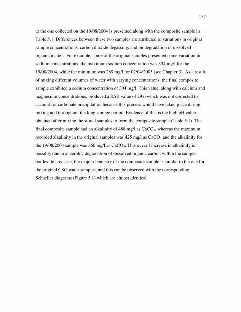
157
to the one collected on the 19/08/2004 is presented along with the composite sample in
Table 5.1. Differences between these two samples are attributed to variations in original
sample concentrations, carbon dioxide degassing, and biodegradation of dissolved
organic matter. For example, some of the original samples presented some variation in
sodium concentrations: the maximum sodium concentration was 334 mg/l for the
19/08/2004, while the minimum was 289 mg/l for 02/04/2005 (see Chapter 3). As a result
of mixing different volumes of water with varying concentrations, the final composite
sample exhibited a sodium concentration of 304 mg/l. This value, along with calcium and
magnesium concentrations, produced a SAR value of 29.6 which was not corrected to
account for carbonate precipitation because this process would have taken place during
mixing and throughout the long storage period. Evidence of this is the high pH value
obtained after mixing the stored samples to form the composite sample (Table 5.1). The
final composite sample had an alkalinity of 488 mg/l as CaCO3, whereas the maximum
recorded alkalinity in the original samples was 425 mg/l as CaCO3 and the alkalinity for
the 19/08/2004 sample was 360 mg/l as CaCO3. This overall increase in alkalinity is
possibly due to anaerobic degradation of dissolved organic carbon within the sample
bottles. In any case, the major chemistry of the composite sample is similar to the one for
the original CSG water samples, and this can be observed with the corresponding
Schoeller diagrams (Figure 5.1) which are almost identical.

158
Figure 5.1. Schoeller diagrams for the 19/8/2004 sample and the composite sample (2004-2005) for Maramarua CSG water
Methods
The Ngakuru zeolites capacity to remove sodium ions in solution was assessed
with a preliminary batch study, followed by flow-through tests using an ion exchange
column.
Batch tests Four types of batch tests were carried out as preliminary experiments to determine
the feasibility of using Ngakuru zeolites for the removal of sodium cations from solution,
and for initial sizing calculations. The following tests were carried out in four phases.
Phase I. The first batch tests focused on assessing the sodium removal capacity of
Ngakuru zeolites while evaluating the effects of particle size using 1 M NaCl solutions.
For this purpose, the first set of zeolites was rinsed with deionised water and then dried in
an oven at 100ºC. Samples were then sieved through 150, 300, 600, 1180, and 2360 µm
sieves, and about 1 gram of each of these was placed in conical flasks along with about
50 ml of 1 M NaCl solution. In addition, about 1 gram of pet litter zeolite (unwashed, air-
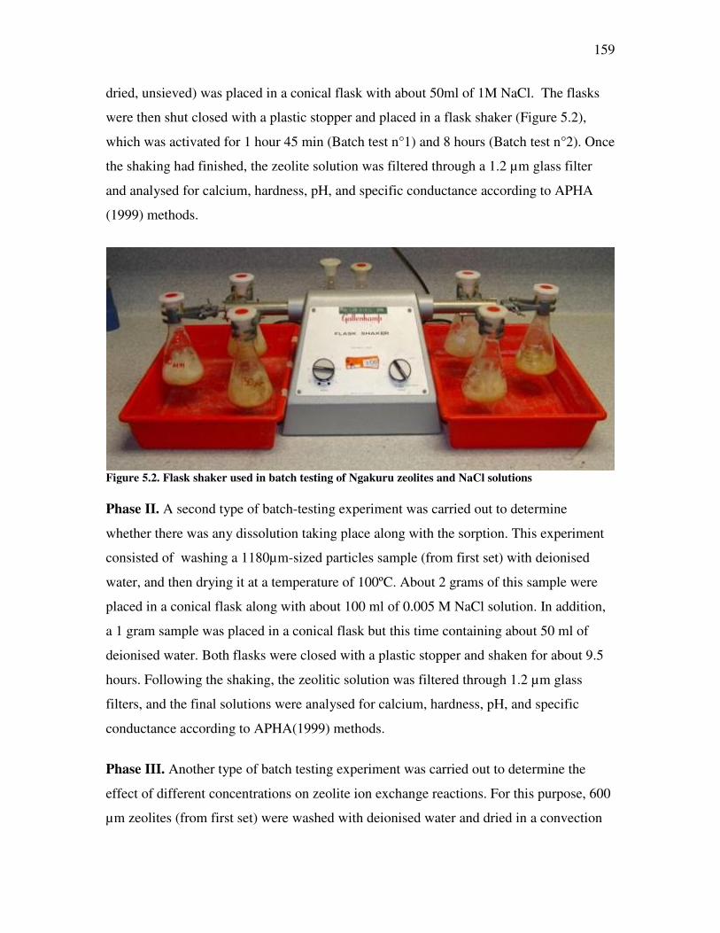
159
dried, unsieved) was placed in a conical flask with about 50ml of 1M NaCl. The flasks
were then shut closed with a plastic stopper and placed in a flask shaker (Figure 5.2),
which was activated for 1 hour 45 min (Batch test n°1) and 8 hours (Batch test n°2). Once
the shaking had finished, the zeolite solution was filtered through a 1.2 µm glass filter
and analysed for calcium, hardness, pH, and specific conductance according to APHA
(1999) methods.
Figure 5.2. Flask shaker used in batch testing of Ngakuru zeolites and NaCl solutions Phase II. A second type of batch-testing experiment was carried out to determine
whether there was any dissolution taking place along with the sorption. This experiment
consisted of washing a 1180µm-sized particles sample (from first set) with deionised
water, and then drying it at a temperature of 100ºC. About 2 grams of this sample were
placed in a conical flask along with about 100 ml of 0.005 M NaCl solution. In addition,
a 1 gram sample was placed in a conical flask but this time containing about 50 ml of
deionised water. Both flasks were closed with a plastic stopper and shaken for about 9.5
hours. Following the shaking, the zeolitic solution was filtered through 1.2 µm glass
filters, and the final solutions were analysed for calcium, hardness, pH, and specific
conductance according to APHA(1999) methods.
Phase III. Another type of batch testing experiment was carried out to determine the
effect of different concentrations on zeolite ion exchange reactions. For this purpose, 600
µm zeolites (from first set) were washed with deionised water and dried in a convection

160
oven at around 100ºC. Four samples of about 2 grams each, were placed in conical flasks
with about 120 ml of concentrated sodium solutions. The solutions used were 1 M, 0.1 M,
and 0.01 M of NaCl plus a 0.01 M solution of NaOH. These flasks were shaken for
approximately 4 hours and, subsequently, the zeolitic solution was filtered through 1.2
µm glass filters. The final solutions were analysed for calcium, hardness, pH, and specific
conductance according to APHA(1999) methods, and also for sodium using a calibrated
Cole-Parmer sodium ion electrode (see Appendix A.1 for a summary of these procedures
and calibration method for the sodium ion electrode).
Phase IV. The objective of the last type of batch testing was to determine whether it was
possible to regenerate Ngakuru zeolites after they had absorbed sodium cations. This also
helped assess how rigid or prone to mechanical breakdown were the zeolites, and to
determine a maximum sodium exchange capacity (useful for preliminary sizing
calculations in the flow-through experiments). To do this, different service/regeneration
cycles were carried out using concentrated sodium solutions for service, and various
calcium, potassium, and acid solutions for regeneration. For example, the first of these
experiments used 1180 µm zeolites which had been previously washed with deionised
water and dried in a convection oven at approximately 100ºC. A 13.4 gram sample was
placed in a conical flask along with 220 ml of a 0.01M NaOH solution, and it was then
shaken continuously for 5 hours. After this period of time, the sample was filtered using a
1.2 µm glass filter, and the final solution was analysed for calcium, hardness, pH, and
specific conductance according to APHA(1999) methods. In addition, sodium
concentration was determined using a calibrated Cole-Parmer sodium ion electrode. The
zeolite sample remaining after filtering was then washed with deionised water, dried in a
100ºC convection oven, and sieved through a 1180 µm sieve. The zeolitic material was
then weighed and placed in a conical flask along with 150ml of 0.1 M HCl solution.
Subsequently, the conical flask was shaken for approximately 5 hours, and at the end of
this period, the sample was filtered using a 1.2 µm glass filter. The final solution was
analysed for calcium, hardness, pH, specific conductance, and sodium. This cycle was
repeated five times with different dissolved salts of varying concentrations, while
analysing the final solutions resulting from each shaking period. In addition, some of

161
these samples were analysed for potassium at the Department of Chemistry (University of
Canterbury) using atomic absorbtion and in accordance to APHA(1999) methods; two of
the samples were analysed for chloride and sulphate using HACH methods 8225 and
8051 (Hach Company, 2003). Similar experiments like the one just mentioned were
carried out, but with different solutions and with both 1180 and 600 µm particle sizes.
Table 5.2 summarises these batch test experiments and their corresponding
service/regeneration cycles.
Table 5.2. Summary of batch tests to assess zeolite regeneration potential in Phase IV Experiment number
Cycle phase Particle size
Zeolite weight
Dissolved salt
Concentration Volume Analyses after shaking
(µm) (g) M ml 1 Service 1180 13.4 NaOH 0.01 220 Typical Regeneration 1180 8.5 HCl 0.1 150 Typical Service 1180 7.1 NaOH 0.01 130 Typical Regeneration 1180 4.6 HCl 1 125 Typ. +Cl- +SO4
2- Service 1180 3.8 NaOH 0.01 125 Typ. +Cl- +SO4
2- Regeneration 1180 3.4 CaCl2 0.09 125 Typical + K+ Service 1180 3.0 NaCl 0.01 125 Typical + K+ Regeneration 1180 2.7 CaCl2 0.01 125 Typical + K+ Service 1180 2.5 NaCl 0.01 125 Typical + K+ Regeneration 1180 2.2 KCl 0.1 125 Typical Service 1180 2.1 NaCl 0.01 125 Typical + K+ 2 Service 600 4.0 NaCl 0.01 225 Typical + K+ Regeneration 600 2.7 HCl 1 125 Typical Service 600 2.1 NaCl 0.01 125 Typical Regeneration 600 1.9 CaCl2 0.09 125 Typical + K+ Service 600 1.8 NaCl 0.01 125 Typical + K+ Regeneration 600 1.7 CaCl2 0.01 125 Typical Service 600 1.6 NaCl 0.01 125 Typical Regeneration 600 1.5 KCl 0.1 125 Typical Service 600 1.4 NaCl 0.01 125 Typical + K+ 3 Service 1180 2.0 NaCl 0.01 125 Typical + K+ Regeneration 1180 1.2 CaCl2 0.09 125 Typical Service 1180 1.0 NaCl 0.01 125 Typical + K+ Regeneration 1180 0.8 CaCl2 0.01 125 Typical Service 1180 0.7 NaCl 0.01 125 Typical Regeneration 1180 0.6 KCl 0.1 125 Typical 4 Service 1180 2.0 NaCl 0.01 125 Typical + K+ Regeneration 1180 1.0 CaCl2 0.01 125 Typical + K+ Service 1180 0.8 NaCl 0.01 125 Typical + K+ Regeneration 1180 0.7 KCl 0.1 125 Typical 5 Service 1180 2.1 NaCl 0.01 125 Typical + K+ Regeneration 1180 1.2 KCl 0.1 125 Typical Notes: 1. After each cycle phase samples were dried in a convection oven at around 100ºC, and sieved prior to starting
the next phase 2. Zeolite samples correspond to the ones from set 1 3. Typical analyses are: pH, Specific conductance, calcium, hardness, and sodium

162
Flow-through tests
The objective of column tests, or flow-through tests, was to determine the sodium
exchange capacity of Ngakuru zeolites in laboratory experiments resembling field-
operating conditions. This also helped to determine the efficiency of the process and the
optimal operating mode.
Flow-through tests involved the use of a zeolite-packed column with feed solution
running through it. The column used in these experiments was especially designed and
manufactured at the University of Canterbury, and it consisted of a 3 mm glass tube of
about 75 cm in length, with a funnel attached to one of its openings. In addition, this
column had a sintered glass filter at the funnel, and two taps for controlling flow in and
out of the column (Figure 5.3). Most of the experiments with the ion exchanged column
used about 240 g of zeolite material, but about 180 g were used in Experiment N°7.
Figure 5.3. Glass column used in flow-through experiments

163
The first flow-through experiments were carried out in downflow mode, but this
led to channelling and preferential flow so, to avoid these problems, it was decided to run
the column in upflow mode for most of the experiments. In downflow mode, the feed
solution was supplied through gravity dripping by a reservoir located over the glass
column. This reservoir had an adjustable tap which enabled the selection of desired flow
rates. In upflow mode, the feed solution was supplied through a 10mm plastic tube
attached to the bottom tap. The other end of the tube fed directly into a container holding
the feed solution, which was fed into the column with the aid of a peristaltic pump. This
pump had a control dial allowing it to regulate flow rate, which was useful throughout the
different modes of operation (the average retention time was about 14 minutes).
Typical operation mode included service, backwash, regeneration, and rinse.
Service was carried out either in upflow or downflow mode at a specified flow rate, while
backwash was carried out with deionised water at a high flow rate (as high as 180
cm3/min) and always in upflow mode. Regeneration was carried out in the same direction
of flow and same rate as in service mode using 1 litre KCl (1 M) and CaCl2 (0.044 M)
solutions. The next step was the rinsing step, which was necessary to remove any excess
regenerant prior to service. This step was carried out with deionised water in upflow
mode and at two different flow rates – a slow rate (as slow as the regeneration rate) to
displace excess regenerant from the zeolite bed, and a fast rate (about twice as fast) to
remove any residual solution from the zeolites. After rinsing, the bottom tap of the
column was opened to drain any remaining liquid from the column. The complete cycle
was carried out only when using regeneration - when solely carrying out service tests, the
cycle was interrupted and used zeolites were discarded. In addition, one of these
experiments was carried out with a warmed feed solution (~40°C) to determine if
efficiency improved significantly with higher temperatures. Table 5.3 summarises the
different experiments and provides relevant details.

164
Table 5.3. Summary of flow-through experiments N° Experiment type Feed Solution Direction
of flow Flow Rate
Feed volume
Zeolites particle size
Zeolites Mass
Retention Time
cm3/min litres (µm) grams min 1 No prior regeneration 0.01 M NaCl downflow 21-26 10.1 1180 269.7 13.2 2 No prior regeneration 0.1 M NaCl downflow 33 1.8 600 240.0 8.4 3 Prior regeneration with
1M KCl (1litre) and zeolites from experiment n° 2
0.1 M NaCl upflow 13-19 1.83 600 240.0 17.4
4 No regeneration but
feed solution was heated to ~40°C
0.1M NaCl upflow 13-19 1.5 300 240.1 17.1
5 No prior regeneration 0.044M NaCl upflow 12-21 2.7 600 240.1 16.1 6 Prior regeneration with
0.044M CaCl2 (1 litre) and zeolites from experiment n° 5
0.044 M NaCl upflow 14-20 2.7 600 240.1 15.6
7 No prior regeneration Maramarua CSG water Equivalent to 0.013 M NaCl (1)
upflow 15-17 4.53 600 180.0 11.3
(1) Equivalent concentration was calculated using the composite sample (Table 5.1) with sodium concentrations of 304 mg/l. Differences in specific conductance and chloride concentrations are assumed negligible in this conversion. During experiment n°4, the feed solution was heated to 100°C, but it cooled down
while being pumped into the column, entering it at a temperature of approximately 40°C.
The original NaCl concentration was 0.1M, but this could have increased because of
water evaporation from the heated beaker. In addition, the zeolites were washed with
deionised water inside the column before the experiment started. This was done to keep
the zeolite bed moist in order to promote saturated flow at the start of the test.
In experiments n° 1, 2, 4, and 5 (Table 5.3) zeolites were prewashed with
deionised water before each service run. Experiments n° 3, 5, and 6 tested regenerated
zeolites that had previously been used in experiments n° 2, 4, and 5 respectively, so no
pre-washing was carried out (except for the rinsing after the regeneration cycle).

165
Experiment n°7 was carried out without any pre-washing and with no previous
regeneration.
In each of these experiments, 100 ml aliquots were collected during service runs
either from the top tap (upflow mode) or bottom tap (downflow mode). These aliquots
were stored in sample bottles and analysed after the service run had finalised. Before
analysis, samples were filtered using 1.2 µm glass filters. Basic analyses carried out at the
Environmental Engineering Laboratory (EEL, University of Canterbury) included pH,
specific conductance, calcium, and hardness, which were carried out according to the
methods outlined in APHA (1999). Also, sodium concentrations were determined using a
calibrated Cole-Parmer sodium ion electrode. For experiments n° 6 and 7 (Table 5.3)
samples were analysed for pH and specific conductance at the EEL, and then sent to Hill
Laboratories for a complete analysis.
Data from flow-through experiments allowed for the construction of breakthrough
curves showing the sodium absorption capacity of Ngakuru zeolites. This allowed for the
calculation of the total number of exchanged sodium cations for a given mass of zeolites,
while taking into account the interaction of other ions (Ca2+, Mg2+, H+). Further
interpretation of data included calculating and plotting absorption isotherms, and
comparing these to other isotherms from known equilibrium relationships. In addition, it
is possible to calculate the separation factor, r, for the whole isotherm (or R for a section
of the isotherm) to determine the type of reaction taking place in relation to absorption
kinetics. A description of the assumptions and calculation procedures used in these
calculations is presented in Appendix D (section D.1).
Results
Batch test results Phase I. Results for this experiment are presented in Appendix D (Tables D.1 and D.2).
Different particle sizes produced zeolitic solutions having approximately the same
hardness and calcium concentrations. However, a minor trend was noticed where
exchanged cations seemed to increase slightly with fine particle size (passing 150 µm and
retained on the 150 µm sieve) and with coarser sizes (1180 µm and 2360 µm). This can
be observed by analysing the plots of calcium concentrations vs. particle size in Figure

166
5.4. In theory, smaller particle sizes have more surface area and would offer best ion
exchange results, but this was not noticeable in these experiments. Small particles tend to
become buoyant during experiments, and this produces operational problems; larger
particles do not have as much buoyancy as smaller ones, but the same amount of material,
consisting of larger particles, has less surface area available for the exchange. In these
experiments, particle size did not pose a major influence in ion exchange processes.
Figure 5.4 also shows that shaking time does have an influence on reaction kinetics as the
zeolitic solutions that were shaken for 8 hours have more calcium ions than the solutions
that had been shaken for just 1.75 hours. Hardness analyses ( Table D.1, Appendix D)
also showed that zeolitic solutions that had been shaken for 8 hours released more
calcium and magnesium (hardness) than the ones shaken for just 1.75 hours. In addition,
the pet litter zeolite sample that was shaken for 1.75 hours produced significantly lower
concentrations of calcium ions in solution (46 mg/l/g) than the zeolitic solutions shaken
for the same period of time but containing zeolites from set n°1 (78-99 mg/l/g zeolites).
There was no pattern in pH changes for the different shaking times and particle sizes
being tested (pH 4.5-5.7). This analysis also helps to make initial “go” or “no go”
decisions when working with a new material. In this case pet litter exchanged less
calcium than high-grade zeolites, and this suggests pet litter contains less ion exchange
minerals (i.e. mordenite) than high grade zeolites. Since calcium determination is simple,
accurate, and fast, this can save time and money during the initial assessment of an ion
exchange material. Based on these results it was decided to work with high-grade zeolites
with a medium ranged particle size (300 or 600 µm).

167
Calcium concentration after vigorous shaking
405060708090
100110120130
Passing150 um
150 um 300 um 600 um 1180 um 2360 umZeolite particle size
mg
/l/g
of z
eolit
e
Batch test N°1. Shaking time: 1hour 45 min
Batch test N°2. Shaking time: 8 hours
Figure 5.4 Phase II. Results for this experiment are presented in Table D.3 (Appendix D). Shaking
for 9.5 hours with low concentration NaCl solution (0.005 M) revealed that there was
little or no change in specific conductance (from 538 to 546 µS/cm), and some calcium (8
mg/l) and hardness (32 mg/l as CaCO3) were detected at the end of the shaking time. In
addition, pH decreased from 6.2 to 5.5, which suggests that hydrogen ions were being
exchanged for sodium. When using deionised water, results indicated very small amounts
of calcium (3.2 mg/l) and hardness (4.2 mg/l as CaCO3) being released, and a slight
increase in specific conductance (from 1.9 to 41.8 µS/cm). The pH of this sample was 6.4
indicating little or no difference from the original pH of deionised water (pH 7). These
results suggest that some dissolution could be taking place, but at this stage it was not
possible to measure the magnitude of this (albeit low) dissolution. If the reaction taking
place had been solely an ion exchange reaction, specific conductance would have
remained the same, and few cations would have been detected in the deionised water with
the zeolites.
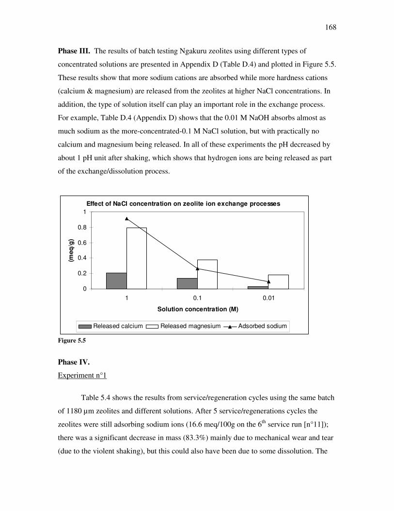
168
Phase III. The results of batch testing Ngakuru zeolites using different types of
concentrated solutions are presented in Appendix D (Table D.4) and plotted in Figure 5.5.
These results show that more sodium cations are absorbed while more hardness cations
(calcium & magnesium) are released from the zeolites at higher NaCl concentrations. In
addition, the type of solution itself can play an important role in the exchange process.
For example, Table D.4 (Appendix D) shows that the 0.01 M NaOH absorbs almost as
much sodium as the more-concentrated-0.1 M NaCl solution, but with practically no
calcium and magnesium being released. In all of these experiments the pH decreased by
about 1 pH unit after shaking, which shows that hydrogen ions are being released as part
of the exchange/dissolution process.
Effect of NaCl concentration on zeolite ion exchange processes
0
0.2
0.4
0.6
0.8
1
1 0.1 0.01
Solution concentration (M)
(meq
/g)
Released calcium Released magnesium Adsorbed sodium
Figure 5.5
Phase IV.
Experiment n°1
Table 5.4 shows the results from service/regeneration cycles using the same batch
of 1180 µm zeolites and different solutions. After 5 service/regenerations cycles the
zeolites were still adsorbing sodium ions (16.6 meq/100g on the 6th service run [n°11]);
there was a significant decrease in mass (83.3%) mainly due to mechanical wear and tear
(due to the violent shaking), but this could also have been due to some dissolution. The

169
last column in Table 5.4 shows the exchange that has taken place between the zeolite and
the main cations originally in solution (Na+, Ca2+, K+, or H+).
Chemical analyses of sample solutions revealed the nature of the ion exchange
processes taking place during shaking. The first batch service run (n°1) showed that the
original zeolite material contains calcium (0.07 meq/l) and magnesium (0.04 meq/l) as
occluded salts. These results are consistent with the calcium and magnesium (hardness)
concentration obtained during the first phases. After the first regeneration (with HCl in
n°2) a maximum magnesium concentration of 2.85 meq/l was detected in the solution
after the exchange. It was possible to verify that magnesium remained within the zeolite
even after a few service/regeneration runs (n° 3, 5, 6, 7, and 8); when regenerating with a
higher valence regenerant (Ca2+ in n°6), magnesium concentrations in solution increased
to 2.01 meq/l even though the previous service run had yielded a low magnesium
concentration value (0.08 meq/l). Similar results were obtained with calcium - these
cations were released during the first service run and during the two following
service/regeneration cycles (n° 1-5). The maximum calcium concentration was detected
during the first regeneration run (n°2, 5.9 meq/l) and after regenerating with a strong acid
(n°4, 2.0 meq/l). Thereafter more calcium cations were released but these were mainly a
product of regenerating with CaCl2 in regeneration run n°6 (172 meq/l). In sum, during
each service run sodium cations were adsorbed by the zeolites, while calcium,
magnesium, potassium, and some hydrogen ions were released; during regeneration, the
opposite exchange is taking place – hydrogen, calcium, or potassium ions are being
exchanged for sodium ions in the zeolite.
Throughout all of the service runs in Table 5.4, pH values decreased considerably
after each run. This indicated that hydrogen ions were being released from the zeolites as
part of the exchange process. For example, after the first service run, pH values decreased
from 11.23 to 9.91, and after the last service run these values decreased from 6.34 to 4.64.
A pH decrease of almost 7-fold was detected after service runs n° 3 and n°5 (from 11.23
down to 4.77 and 4.01), but this is due to HCl being used in the previous regeneration
runs.
Unfortunately, it was not possible to measure potassium during the first service
run and the following 2 service/regeneration runs, but it was possible to measure

170
potassium cations in some of the subsequent samples. Results indicated that there is some
potassium originally present in the zeolite material, and that this is slowly being released
with each service/regeneration run. The fourth service run (n°7 in Table 5.4) produced a
solution with 0.2 meq/l of K+ cations, while the fifth service run (n°9 in Table 5.1)
produced 0.1 meq/l of K+. The last service run produced more potassium (3.1 meq/1), but
this is a product of previous KCl regeneration.
Chloride and sulphate were measured after runs n° 4 and 5 to determine whether
dissolution of these anions was taking place. In both instances, sulphate concentrations
were nil. A difference of 8.6% was detected in chloride concentrations after regenerating
with 1M HCl in run n°4.

171
Table 5.4. Experiment n°1. Batch sorption experiments with 1180µm zeolites n° Reaction
type zeolite weight
sample volume
Sol. type
initial pH
final pH
final Na+
final Ca2+
final Mg2+
final K+
trapped cations(2)
released cations(3)
charge balance(4)
main cation exchange(5)
g litres meq/l meq/l meq/l meq/l meq/l meq/l meq/l meq/100g 1 Service 13.36 0.220 0.01M
NaOH 11.23 9.91 3.4 0.07 0.04 NA 6.6 6.6 0.0 10.8
2 Regeneration 8.54 0.150 0.1M HCl
1.12 1.33 15.9 5.9 2.85 NA 38 24.6 13.7 27.9
3 Service 7.13 0.130 0.01M NaOH
11.23 4.77 2.8 0.32 0.12 NA 7.2 7.2 0.0 13.1
4 Regeneration 4.57 0.125 1M HCl
0.25 0.26 9.5 2.0 0.00 NA 11.5 11.5 0.0 26.1
5 Service 3.81 0.125 0.01M NaOH
11.23 4.01 3.5 0.24 0.08 NA 6.5 6.5 0.0 21.2
6 Regeneration 3.35 0.125 0.09M CaCl2
5.32 4.06 1.0 172 2.01 0.0 4.0 3.2 0.8 3.9
7 Service 3.03 0.125 0.01M NaCl
6.34 3.21 8.8 0.36 0.04 0.2 1.2 1.3 0.1 5.0
8 Regeneration 2.72 0.125 0.01M CaCl2
6.62 4.7 0.5 18 0.60 0.0 2.3 1.1 1.2 2.2
9 Service 2.46 0.125 0.01M NaCl
6.34 3.49 8.4 0.4 0.00 0.1 1.6 0.9 0.7 8.0
10 Regeneration 2.23 0.125 0.1M KCl
6.76 3.13 5.4 0.8 0.00 0.0 NA 7.1 NA 30.2
11 Service 2.06 0.125 0.01M NaCl
6.34 4.64 7.3 0.4 0.00 3.1 2.7 3.5 0.7 16.6
Notes: 1) NA = not available 2) Trapped cations for each run:
a. Na+ : n°1, 3, 5, 7, 9, 11 b. H+ : n°2, 4 c. Ca2+ : n°6, 8 d. K+ : n°10
3) Released cations for each run a. n°1, 3, 5, 7, 9, 11:
Mg2+ + Ca2+ + K+ + H+ b. n°2: Mg2+ + Ca2+ + Na+ c. n°4: Mg2+ + Ca2+ + K+ + Na+ d. n°6, 8: Mg2+ + H+ + K+ + Na+ e. n°10: Mg2+ + Ca2+ + Na+ + H+
4) Charge balance = released cations – trapped cations 5) Main cation exchange (MCE) = meq of main cation
intervening in the exchange reaction per 100g of zeolites
)()()/(100
gramsweightZeolitelvolumeSamplelmeqionExchanged
MCE⋅⋅=
172
Experiment n°2 This experiment was very similar to experiment n°1 except in this case 600 µm
zeolites were used instead of 1180 µm, and the only type of solution used during service
was NaCl. Likewise, results from this experiment were similar to the results obtained in
the previous experiment. Experiment n°2 results and observations are presented in
Appendix D.
Experiment n°3-n°5
Experiments n°3-n°5 aimed at reproducing the results obtained in experiment n°1.
The results from these experiments are presented in Tables D.6-D.8 in Appendix D. In
these experiments, 1-3 service/regeneration cycles were done with 1180 µm zeolites. The
decrease in zeolite mass (due to shaking) was 73%, 65%, and 46% for 3, 2, and 1 cycles
respectively.
On average, there was a concentration of calcium of about 0.62 meq/l being
released from the zeolites during the first service run in each of these experiments.
Similarly, average concentrations of magnesium (0.23 meq/l) and potassium (0.50 meq/l)
showed that these zeolites were releasing the same number of cations when exposed to
the same volume of NaCl concentrated solution (0.01M).
Throughout these experiments, pH tended to decrease after each service or
regeneration run, which shows that hydrogen ions are being released as part of the
exchange. However, pH tended to increase slightly after the first service run in each of
these experiments, which indicates that hydrogen ions might have been absorbed by the
zeolites but only during the first run (Tables D.6-D.8 in Appendix D).
Since it was not possible to measure potassium concentrations in most of these
experiments, charge balance results are not always available. However, charge balance
for those samples with known potassium concentrations, indicate an average charge
excess of 1.06 meq/l.

173
Flow-through tests
Experiments n°1 and n°2 The first two flow-through experiments (n°1 and n°2 in Table 5.3) produced good
results, but these were carried out in downflow mode which generated preferential flow
as the feed solution entered the packed zeolite column. It was suspected this led to
inefficiencies in zeolite utilisation, therefore these experiments were regarded as
preliminary, and analyses of the 100 ml aliquots were done on a limited number of
samples. Nevertheless, these experiments provided important information and operational
experience to be used through out the rest of the experimental work. Results from
experiments n°1 and n°2 are presented in Appendix D (Tables D.9 & D.10 and Figures
D.2 & D.3).
Experiment n°3 This experiment was carried out in upflow mode with KCl-regenerated zeolites
from experiment n°2. In this experiment, 1780 ml of 0.1 M NaCl were run through the
column, producing 18 100 ml-sample aliquots. Chemical analyses for these samples are
presented in Appendix D (Table D.11), and a plot of sodium concentration vs. volume
flowing through the column is presented in Figure D.4 (Appendix D). The total sodium
exchange taking place throughout this experiment was at least 40.9 meq/100g. This value
was calculated by adding the milliequivalences of sodium adsorbed by the zeolites
throughout the duration of the experiment - the remaining sodium concentration was
determined with a calibrated sodium electrode in each aliquot after it had percolated
through the column, since the original concentration and volume of the feed solution are
known then it is possible to calculate the adsorbed sodium (simple subtraction). This
process was carried out for each of the sample aliquots, and these values were then added
together resulting in the total sodium adsorbtion for this experiment (in meq). Since the
zeolite’s weight is known, then this value can be expressed in meq/100g.

174
Experiment n°4 Results for this experiment (no regeneration, feed at 40°C) are presented in
Appendix D (Table D.12). Calcium and magnesium concentrations were calculated for
samples n°1, 3, 10, and 15. Calcium and magnesium concentrations for sample n°3
contained the highest concentrations measured for this experiment, and these
concentrations decreased in samples n°10 (by 46% and 16% respectively) and 15 (35%
and 14% respectively).
A plot of the sodium sorption results is presented in Appendix D (Figure D.4).
Sodium concentrations in the collected samples increased in logarithmic form (R2=0.99)
until reaching the original sodium concentration after 1400 ml of feed solution had gone
through the column. The total sodium absorption was calculated by subtracting the
residual sodium concentration in collected samples from the original sodium
concentration in the feed solution, and by adding these values throughout the duration of
the experiments. At the end of this experiment, the total sodium sorption by Ngakuru
zeolites was 19.3 meq/100g.
Samples in experiment n°4 had pH values in the 4.07-5.38 range consistently
lower than the original pH value of 5.85 (Table D.12 in Appendix D). The pH values for
sample n°2 was the highest pH value recorded, followed by the pH value for sample n°3;
pH values in the following samples stayed fairly constant at an average of 4.14.
Experiment n°5
Experiment n°5 showed that it is possible to absorb sodium ions from a 0.044M
(1000 mg/l) NaCl solution using Ngakuru zeolites. In addition, calcium, magnesium, and
hydrogen ions were released from the zeolites during the exchange process. Results from
this experiment are presented in Table D.13 (Appendix D), and a plot of the sodium
sorption and cation release is presented in Figure D.5 (Appendix D).
The total sodium sorption that took place throughout this experiment was 15.9
meq/100g. The maximum sodium sorption took place at the beginning of the experiment
- sample n°1 had the lowest sodium concentration (14.5 meq/l), but sodium
concentrations in succeeding aliquots increased almost linearly (Figure D.5, Appendix D)
until about 700 ml of feed solution had flowed through the column. From then onwards,

175
sodium concentrations increased logarithmically (Figure D.5, Appendix D) until reaching
a final value of 38.4 meq/l (sample n°27). The relationship between sodium and flow-
through volume can be approximated by a linear trendline with an R2 value of 0.95 (Eq 2,
Appendix D). The total sodium sorption that took place during this experiment was 15.9
meq/100g.
Calcium concentrations in aliquots tended to increase linearly for the first 5
samples (Figure D.5, Appendix D) starting at 10.7 meq/l (sample n°1) and finishing at
12.8 meq/l (sample n°5). However, from then onwards calcium concentrations decreased
in inverse logarithmic form until reaching a final value of 4.8 meq/l in sample n°25.
Similarly, magnesium concentrations were the highest at the beginning of the
experiment, with sample n°1 having a concentration of 14.3 meq/l. However, throughout
this experiment, magnesium concentrations decreased in an inverse logarithmic fashion
(Figure D.5, Appendix D) until reaching a value of 1.1 meq/l (sample n°25).
Throughout this experiment, pH values stayed fairly low and within the 4.45-4.79
pH range. This is almost 2 pH units below the original pH (6.35), and it shows that
hydrogen ions are also taking part of the cation exchange. However, there was no
identifiable trend in pH values as the experiment was being conducted.
Specific conductance of the outflow remained fairly constant throughout this
experiment. The conductance of the untreated feed solution was 5.1 dS/m, and the
conductance of the outflow was very similar and remained fairly unchanged throughout
the different samples measured in this experiment (average = 5.05, ��= 0.06).
Experiment n°6 Experiment n°6 was carried out with regenerated zeolites (using CaCl2) from
experiment n°5. Results for this experiment are presented in Table 5.5, and plots of the
cation exchange process are presented in Figures 5.6 and 5.7.

176
Table 5.5. Results for experiment n°6 Sample vol. through pH Na+ Ca2+ Mg2+ K+ n° ml pH units meq/l meq/l meq/l meq/l 1 100 5.25 11.1 27.2 0.58 1.74 2 200 4.81 15.6 NA NA NA 3 300 4.7 17.0 24.1 0.26 2.38 4 400 4.65 19.1 NA NA NA 5 500 4.67 21.1 20.3 0.17 2.74 6 600 4.93 NA NA NA NA 7 700 4.55 22.7 16.8 0.14 2.79 8 800 4.55 NA NA NA NA 9 900 4.56 26.8 14.0 0.12 3.04 10 1000 4.55 NA NA NA NA 11 1100 4.56 28.7 11.9 0.12 3.10 12 1200 4.56 NA NA NA NA 13 1300 4.57 31.1 10.0 0.10 3.04 14 1400 4.57 NA NA NA NA 15 1500 4.57 31.3 8.5 0.10 2.97 16 1600 4.59 NA NA NA NA 17 1700 4.59 33.3 7.6 0.10 3.02 18 1800 4.61 NA NA NA NA 19 1900 4.62 34.3 6.8 0.11 3.02 20 2000 4.63 NA NA NA NA 21 2100 4.62 35.1 6.2 0.11 2.92 22 2200 4.64 NA NA NA NA 23 2300 4.63 34.8 5.9 0.11 2.86 24 2400 4.63 34.7 NA NA NA 25 2500 4.67 34.5 5.2 0.11 2.76 26 2600 4.84 NA NA NA NA 27 2700 4.84 35.8 4.9 0.12 2.81
Notes: 1) Feed solution is a 0.044 M NaCl solution with pH= 5.85 2) Original Na+ concentration is 0.044 M (1000 mg/l = 43.5 meq/l) 3) Na+, Ca2+, Mg2+, and K+ concentrations were measured through Hill
Laboratories 4) Ca2+: 1 meq/l = 20.04 mg/l; Mg2+: 1 meq/l = 12.15 mg/l; K+:1 meq/l = 39.1
mg/l 5) Aliquot volume is 100 ml 6) For further information about experiment setup refer to Table 5.3 7) NA = no data available
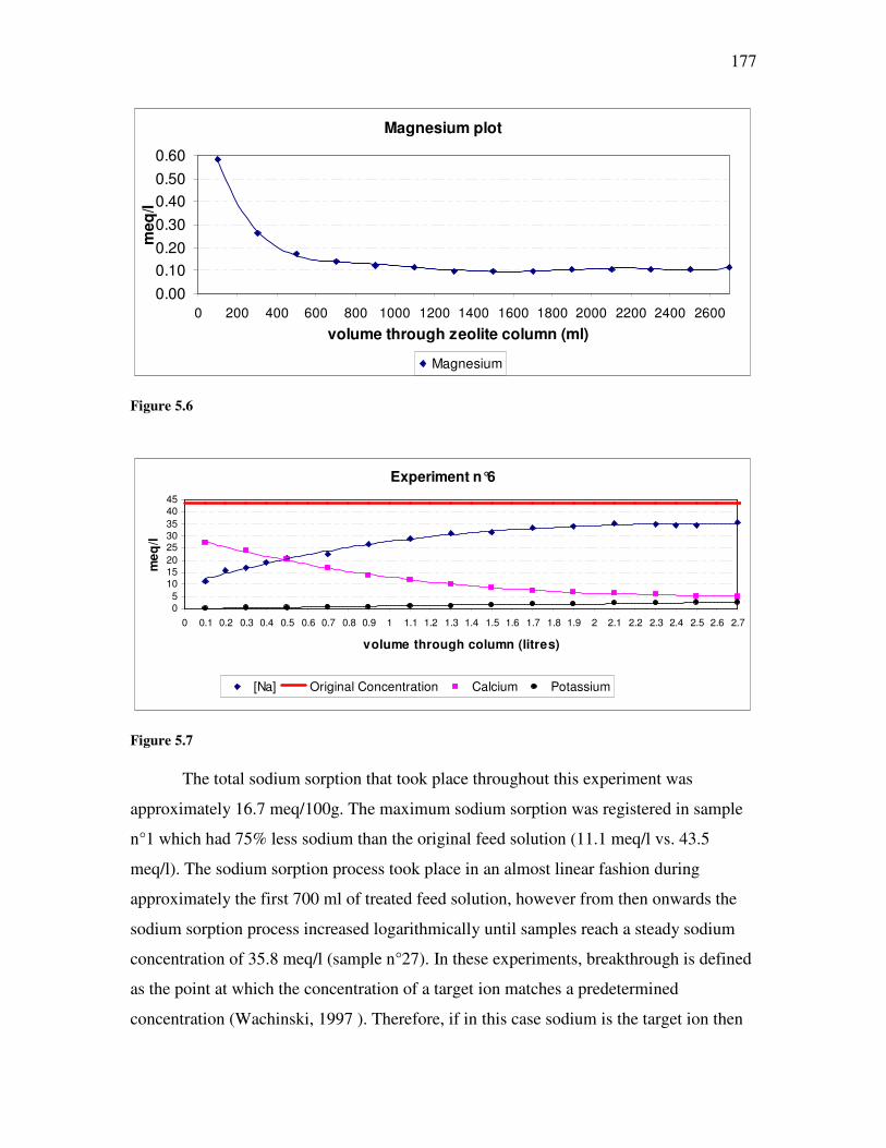
177
Magnesium plot
0.000.100.200.300.400.500.60
0 200 400 600 800 1000 1200 1400 1600 1800 2000 2200 2400 2600
volume through zeolite column (ml)
meq
/l
Magnesium
Figure 5.6
Experiment n°6
05
1015202530354045
0 0.1 0.2 0.3 0.4 0.5 0.6 0.7 0.8 0.9 1 1.1 1.2 1.3 1.4 1.5 1.6 1.7 1.8 1.9 2 2.1 2.2 2.3 2.4 2.5 2.6 2.7
volume through column (litres)
meq
/l
[Na] Original Concentration Calcium Potassium
Figure 5.7 The total sodium sorption that took place throughout this experiment was
approximately 16.7 meq/100g. The maximum sodium sorption was registered in sample
n°1 which had 75% less sodium than the original feed solution (11.1 meq/l vs. 43.5
meq/l). The sodium sorption process took place in an almost linear fashion during
approximately the first 700 ml of treated feed solution, however from then onwards the
sodium sorption process increased logarithmically until samples reach a steady sodium
concentration of 35.8 meq/l (sample n°27). In these experiments, breakthrough is defined
as the point at which the concentration of a target ion matches a predetermined
concentration (Wachinski, 1997 ). Therefore, if in this case sodium is the target ion then

178
sample n°21 corresponds to the breakthrough point (35.1 meq/l). The best fit for these
data is given by a logarithmic equation with an R2 value of 0.98 (Eq 5.1).
litresin column through volume (meq/l)aliquot samplein ion concentrat sodium [Na]
where,
9.27)ln(8.1 [Na]
==
+×=
v
v
Eq 5.1 Calcium concentrations decreased logarithmically throughout this experiment
(Figures 5.6 and 5.7), but the best fit is given by a third order polynomial equation
(R2=0.999). Calcium concentrations at the start of the experiment are as high as 27.2
meq/l (sample n°1), but at the end of this experiment calcium concentrations reached a
low value of 4.9 meq/l (sample n°27).
On the other hand, magnesium concentrations are very low in comparison to
calcium concentrations throughout this experiment (Table 5.5 and Figure 5.6).
Magnesium concentrations at the start of the experiment were about 29.1 mg/l as CaCO3
(0.58 meq/l), from then onwards magnesium concentrations decreased logarithmically
and, after about 1000ml of feed solution had flowed through the column, magnesium
concentrations stabilised at value of around 0.11 meq/l.
Potassium concentrations in aliquots were fairly constant throughout this
experiment averaging 2.8 meq/l. The minimum potassium concentration was 1.74 meq/l
and it occurred at the start of the experiment (sample n°1).
Throughout this experiment, pH values stayed below the original pH value of 5.85.
The first sample had the highest pH value (5.25), and subsequent pH values stayed below
the 5.0 mark. After 600 ml of treated feed solution, pH values remained constant at
around 4.6, however the last two samples of this experiment showed a slight pH increase
(4.84).
Specific conductance remained constant throughout this experiment. The
conductance of the untreated feed solution was 5.0 dS/m, and this value remained fairly
unchanged throughout the different outflow samples measured in this experiment
(average = 5.11 dS/m, ��= 0.13).
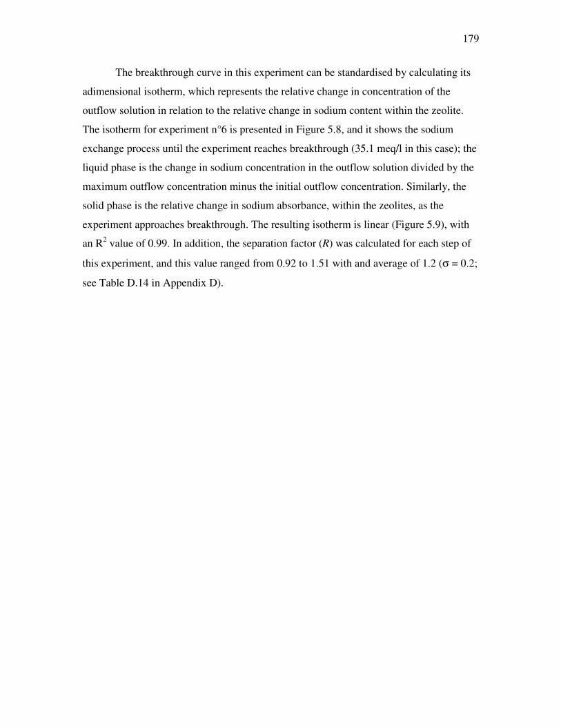
179
The breakthrough curve in this experiment can be standardised by calculating its
adimensional isotherm, which represents the relative change in concentration of the
outflow solution in relation to the relative change in sodium content within the zeolite.
The isotherm for experiment n°6 is presented in Figure 5.8, and it shows the sodium
exchange process until the experiment reaches breakthrough (35.1 meq/l in this case); the
liquid phase is the change in sodium concentration in the outflow solution divided by the
maximum outflow concentration minus the initial outflow concentration. Similarly, the
solid phase is the relative change in sodium absorbance, within the zeolites, as the
experiment approaches breakthrough. The resulting isotherm is linear (Figure 5.9), with
an R2 value of 0.99. In addition, the separation factor (R) was calculated for each step of
this experiment, and this value ranged from 0.92 to 1.51 with and average of 1.2 (σ = 0.2;
see Table D.14 in Appendix D).

180
Sodium Absorption Isotherm - Experiment N°6
y = 0.94x + 0.03R2 = 0.99
0.00
0.20
0.40
0.60
0.80
1.00
0.00 0.10 0.20 0.30 0.40 0.50 0.60 0.70 0.80 0.90 1.00
Liquid phase
So
lid p
has
e
Figure 5.8. Fractional solid-concentration isotherm for experiment n°6.
''''''''
,03.094.0
qqqq
Q
cccc
C
Where
CQ
−−=
−−=
+×=
c = outflow concentration c’= minimum outflow concentration (first sample, 11.1 meq/l ) c’’ = maximum outflow concentration (breakthrough, 35.1 meq/l) q = sodium ion in zeolite q’ = initial zeolite sodium absorption (3.2 meq) q’’ = total zeolite absorption (at breakthrough, 35.0 meq) Figure 5.9 Experiment n°7 Experiment n°7 was carried out with actual CSG water from Maramarua (Table
5.1). The same cations analysed in the previous experiments, were also analysed in
experiment n°7, but in this case a more thorough analysis was carried out in 4 of the
samples to compare these against the original feed solution (Table 5.1). Major cation
exchange results and properties for aliquots throughout this experiment are presented in
Table 5.6, and detailed analyses for selected samples are presented in Table 5.7.

181
�Table 5.6. Column test results for experiment n°7
Sample vol. through pH Sp. Conductance
Na+ Ca2+ Mg2+ K+
n° ml pH units dS/m meq/l meq/l meq/l meq/l 1 103 6.45 2.11 5.4 3.5 12.51 0.7 2 207 7.03 1.42 4.5 2.4 7.91 0.6 3 309 7.09 1.20 4.4 1.9 5.78 0.6 4 409 7.26 1.15 4.8 1.9 5.06 0.7 5 509 7.40 1.15 5.2 2.0 4.39 0.7 6 610 7.51 1.16 5.8 2.1 3.90 0.8 7 710 7.63 1.17 6.2 2.1 3.52 0.8 8 810 7.51 1.18 6.5 2.2 3.13 0.9 9 911 7.78 1.18 6.6 2.1 2.75 0.9 10 1012 7.88 1.19 7.6 2.2 2.63 1.0 11 1113 8.00 1.20 8.3 2.2 2.51 1.0 12 1216 7.85 1.21 8.4 2.2 2.28 1.0 13 1317 7.96 1.22 8.1 2.2 1.95 1.0 14 1418 7.99 1.22 8.7 2.1 1.84 1.0 15 1519 7.92 1.23 9.1 2.1 1.80 1.1 16 1620 8.02 1.23 9.2 2.1 1.61 1.0 17 1724 8.08 1.23 8.4 2.0 1.33 1.0 18 1825 7.98 1.24 9.2 2.0 1.27 1.1 19 1926 8.07 1.24 9.4 2.0 1.23 1.2 20 2027 8.03 1.24 9.4 1.9 1.15 1.2 21 2128 8.11 1.24 9.9 1.9 1.13 1.1 22 2229 8.04 1.25 9.7 1.8 1.04 1.1 23 2330 8.11 1.25 9.4 1.8 0.91 1.1 24 2430 8.14 1.25 10.0 1.8 0.90 1.2 25 2531 8.09 1.26 9.9 1.8 0.83 1.1 26 2632 8.15 1.26 9.5 1.7 0.76 1.1 27 2733 8.20 1.26 9.5 1.8 0.74 1.2 28 2834 8.17 1.26 9.6 1.7 0.67 1.1 29 2934 8.14 1.27 10.2 1.7 0.69 1.2 30 3038 8.19 1.27 NA NA NA NA 31 3138 8.23 1.27 9.5 1.6 0.58 1.1 32 3243 8.20 1.28 NA NA NA NA 33 3343 8.24 1.28 9.6 1.6 0.53 1.1 34 3443 8.28 1.27 NA NA NA NA 35 3543 8.26 1.28 9.6 1.6 0.49 1.1 36 3645 8.29 1.28 10.0 1.6 0.50 1.2 37 3746 8.31 1.28 10.0 1.5 0.47 1.2 38 3846 8.30 1.29 NA NA NA NA 39 3947 8.33 1.29 9.7 1.4 0.42 1.1 40 4046.5 8.33 1.29 NA NA NA NA 41 4146.5 8.32 1.29 10.1 1.4 0.41 1.2 42 4248.5 8.36 1.29 NA NA NA NA 43 4350.5 8.32 1.29 9.8 1.4 0.36 1.1 44 4450.5 8.33 1.29 NA NA NA NA 45 4530.5 8.36 1.29 10.5 1.4 0.37 1.2
Notes: 1) Feed solution is Maramarua CSG water (composite samples, Table 5.1) having a Na
concentration of 13.2 meq/l (1000 mg/l = 43.5 meq/l) and pH= 8.57 2) Na+, Ca2+, Mg2+, and K+ concentrations were measured through Hill Laboratories 3) Ca2+: 1 meq/l = 20.04 mg/l; Mg2+: 1 meq/l = 12.15 mg/l; K+:1 meq/l = 39.1 mg/l 4) Aliquot volume is ~100 ml 5) For further information about experiment setup refer to Table 5.3 6) NA = no data available
�
�
�
�

182
Table 5.7. Full analyses for selected samples (experiment n°7) Samples (1) Unit n°1 n°7 n°19 n°36 Total alkalinity mg/l as
CaCO3 278 428 468 498
Bicarbonate mg/l 339(2) 519(2) 561(2) 590(2) Chloride mg/l 164 151 147 149 Total Organic Carbon
mg/l 216 <0.5 27.7 30.7
Carbonate mg/l 0.1(2) 1.5(2) 4.6(2) 8.2(2) Dis. carbon dioxide mg/l 390(2) 41(2) 16(2) 10(2) Reactive silica mg/l 25.1 27.6 27.1 25.5 Sulphate mg/l 28.0 3.3 2.9 2.9 Total boron mg/l 67.4 2.8 2.6 2.0 Fluoride mg/l 0.23 0.94 1.68 1.28 Dissolved iron mg/l <0.02 <0.02 0.02 0.03 Total iron mg/l <0.4 <0.4 <0.4 <0.4 Dissolved manganese
mg/l 1.96 0.33 0.07 0.0121
Total manganese mg/l 1.89 0.33 0.07 0.02 Total aluminium mg/l <0.06 <0.06 0.09 0.15 Total cobalt mg/l 0.005 <0.004 <0.004 <0.004 Total chromium mg/l <0.01 <0.01 <0.01 <0.01 Total nickel mg/l 0.02 <0.01 <0.01 <0.01 Total nitrogen mg/l NH4-N 0.03 NA NA NA Total zinc mg/l 0.74 0.05 0.03 <0.02
Notes: (1) Samples analysed through Hill Laboratories, Hamilton, New Zealand (2) Calculated using from carbonate chemistry using alkalinity and pH values
�
Throughout this experiment, the total sodium sorption that took place was
approximately 11.3 meq/100g. According to the experimental results in Table 5.6, the
first two aliquots presented higher sodium concentrations than the third one, which was
the sample with the lowest sodium concentration. In any case, sodium concentration for
the first two samples were still very low in comparison to the initial sodium concentration
(41% and 34% for samples n°1 and n°2 respectively). From sample n°3 onwards, sodium
concentrations in aliquots increased in an quasi logarithmic fashion reaching a limit of
approximately 10.0 meq/l (76% of original concentration). This can be observed in

183
Figure 5.10, where sodium concentrations in samples throughout this experiment are
represented by a logarithmic trendline (Eq 5.2) with an R2 value of 0.87.
Sorption results for experiment n°7
0
2
4
6
8
10
12
14
0 0.2 0.4 0.6 0.8 1 1.2 1.4 1.6 1.8 2 2.2 2.4 2.6 2.8 3 3.2 3.4 3.6 3.8 4 4.2 4.4 4.6
Volume through column (litres)
meq
/l
[Na] Original Concentration Calcium Magnesium Figure 5.10
litresin column through volume (meq/l)aliquot samplein ion concentrat sodium [Na]
where,
61.7)ln(1.92 [Na]
==
+×=
v
v
Eq 5.2
The first two sample aliquots in this experiment have a higher sodium
concentration than aliquots n°3 an n°4, and it will be shown later that this is a
consequence of some initial zeolite dissolution. For this reason, the breakthrough curve is
not perfectly logarithmic. However, as in experiment n°6, it is possible to discard these
first two samples in experiment n°7 and calculate an isotherm until breakthrough is
achieved (10 meq/l). This isotherm is presented in Figure 5.11, and it has a linear
trendline with an R2 value of 0.95. In this figure, the liquid phase is the change in sodium
concentration in the outflow solution (minus the original concentration) divided by the
maximum concentration of the outflow solution (minus the original concentration).
Similarly, the solid phase is the relative change in sodium absorbance, within the zeolites,
as the experiment approaches breakthrough. Figure 5.12 presents the linear relationship
for this isotherm, and its calculation procedure. In this case, the separation factor (R)
ranged from 0.28 to 4.7 for each of the aliquots throughout this experiment with an
average of 1.5 (σ = 0.93; see Table D.15 in Appendix D).

184
Sodium Adsorption Isotherm- Experiment n°7
y = 0.93x - 0.01R2 = 0.95
0.0
0.2
0.4
0.6
0.8
1.0
0.0 0.1 0.2 0.3 0.4 0.5 0.6 0.7 0.8 0.9 1.0
Liquid phase
Sol
id p
has
e
Figure 5.11. Fractional solid-concentration isotherm for experiment n°7.
''''''''
,01.093.0
qqqq
Q
cccc
C
Where
CQ
−−=
−−=
−×=
c = outflow concentration c’= minimum outflow concentration (first sample, 4.4 meq/l ) c’’ = maximum outflow concentration (breakthrough, 10.0 meq/l) q = sodium ion in zeolite q’ = initial zeolite sodium absorption (2.5 meq) q’’ = total zeolite absorption (at breakthrough, 13.1 meq) Figure 5.12
Magnesium and calcium cations in samples collected throughout this experiment
tended to decrease in a quasi-logarithmic manner. Magnesium concentration for the first
sample was the highest recorded (12.51 meq/l), but after about 1200ml of treated feed
solution were collected, magnesium concentrations were lower than 2 meq/l getting as
low as 0.36 meq/l in sample n°43. On the basis of charge, calcium concentrations are not
originally as high as magnesium, but these do not decrease as much. The highest calcium
concentration was 3.5 meq/l and it was recorded in the first sample - subsequent samples
tended to have lower calcium levels averaging around 1.8 meq/l after the third sample.
Potassium concentrations in aliquots throughout this experiment were lower than
1.2 meq/l. The initial potassium concentration was 0.7 meq/l (sample n°1), but this value

185
decreased to a minimum (0.6 meq/l) in the third sample. Potassium concentrations then
increased in a logarithmic fashion stabilizing at around 1.1 meq/l.
Throughout this experiment, pH values increased logarithmically (Figure 5.13;
R2 = 0.97) starting at 6.45 and finishing at 8.36 after 4.5 litres of treated feed solution. For
the first 200 ml of treated feed solution, specific conductance values were higher than in
subsequent samples and higher than in the original feed solution. After the first sample,
specific conductance values decreased linearly from 2.10 dS/m to 1.15 dS/m (sample n°5),
and then gradually increased to a value just higher than the original specific conductance
value (1.26 dS/m; Figure 5.14 ).
pH
3.5
4.5
5.5
6.5
7.5
8.5
9.5
0 1000 2000 3000 4000
pH original pH Log. (pH)
Figure 5.13
1
1.2
1.4
1.6
1.8
2
2.2
0 500 1000 1500 2000 2500 3000 3500 4000 4500
Volume through column (ml)
Sp
ecif
ic c
on
du
ctan
ce
(dS
/m)
Sp Conductance Original Sp Conductance (1.26 dS/m)
Figure 5.14 Thorough analyses for selected samples (Table 5.7) indicate increased
concentrations for some of the original sample constituents in the first sample (sample

186
n°1), but not for the remaining samples (n°7, n°19, and n°36). For example, TOC
increased from 29.2 mg/l in the original feed solution to 216 mg/l in sample n°1, while
dissolved carbon dioxide increased from 5 mg/l to 390 mg/l. Sulphate increased from 2.9
mg/l to 28 mg/l, while boron increased from 2.5 mg/l to 67.4 mg/l. Other sample n°1
constituents which increased in concentrations were chloride, manganese, cobalt, nickel
and zinc, but their rise in concentration was not as great in comparison to the original
feed solution. In any case, for all of these constituents concentrations decreased back to
original levels in samples n° 7, n°19, and n°36.
Throughout this experiment, reactive silica concentrations increased to an average
of 26.3 mg/l in samples n° 1, n° 7, n°19, and n°36. This is about a 153% increase in
concentration in relation to the original feed solution concentration (10.4 mg/l). In
addition, aluminium concentrations showed a marked increase in samples n°19 and n°36
(from non-detectable to 0.15 mg/l), whereas fluoride concentrations decreased slightly on
samples n°1 and n°7 (21% and 86% of original concentrations) but then showed some
increase in samples n°19 and n°36 (153% and 116%).
Alkalinity decreased from 488 mg/l as CaCO3 (original feed solution) to 278 mg/l
as CaCO3 in sample n°1, but subsequent values of alkalinity increased to about the same
concentration as the original feed solution concentration in samples n° 7, n°19, and n°36
(Table 5.7). Consequently, bicarbonate and carbonate concentrations followed a similar
trend in concentration (a decrease followed by an increase).
In some of the earlier experiments it was not possible to calculate the total
sodium absorption capacity (due to lack of data), so the theoretical sodium absorption
was calculated instead. This calculation consisted of integrating the trendline equation
describing its breakthrough, and subtracting this value from the total sodium content over
the treated volume range. This also helped to verify total sodium absorption results when
it was possible to calculate these. Table 5.8 shows the theoretical sodium absorption
values calculated for experiments n°1-7. This calculation procedure provides a good
estimate for the missing value for total sodium absorption in experiment n°1, and it
compares well with the rest of the experiments, except for experiment n°2. The latter
experiment has a difference of 33% between the theoretical value and the value
calculated directly from sample analyses, but these differences could be due to the highly

187
variable results obtained in downflow column operation (channelling and preferential
flow) which might have produced a non-representative trendline.
Table 5.8. Total sodium absorption throughout column test experiments Experiment n° Solution concentration total sodium
absorption theoretical sodium absorption
meq/100g meq/100g 1 0.01 M NaCl 1180 µm NA 13.4 2 0.1 M NaCl 600 µm 17.6 11.8 3 0.1 M NaCl 600 µm 40.9 42.8 4 0.1 M NaCl 300 µm 19.3 21.5 5 0.044 M NaCl 600 µm 15.9 15.0 6 0.044 M NaCl 600 µm 16.7 15.9 7 Maramarua CSG water 3) 11.3 11.7 Notes:
1) Total sodium absorption calculated from remaining sodium concentrations in collected samples
2) Theoretical sodium absorption was calculated by integrating trendline equations and subtracting from the total original concentration over the studied range
3) Equivalent to 0.013 M NaCl
Discussion
Batch tests Batch tests (Phases I, III, and IV) revealed that Ngakuru zeolites were capable of
sorbing sodium cations from concentrated solutions of sodium. This was accompanied by
the release of cations, originally contained within the zeolites, and some loss of zeolite
mass. Particle size posed no significant effects on the overall process (Phase I). The
process by which sodium ions were sorbed into the zeolites can be described as an ion
exchange process, and the additional release of ions from the zeolite structure is mainly a
dissolution process (Phase II). But, how extensive is the dissolution process in relation to
the ion exchange? This question can be answered by closely examining the concentration
of the different ions in solution after each batch test experiment.
First of all, there has to be an ion exchange process taking place between sodium
ions in solution and cations within the zeolite. This is because sodium concentrations in
the remanent solutions were lower than in the original solutions at the start of the batch
tests. The ion exchange process taking place between the zeolites and the sodium solution

188
can be described using Figure 5.15. The arrow pointing towards the zeolite represents the
cations being sorbed by the zeolite (sodium), whereas the arrow pointing away from the
zeolite represents the cations being released (calcium, magnesium, potassium, and
hydrogen) – if these cations are the only ones being released, then the difference (on the
basis of charge) between the sodium cations being sorbed and the sum of potassium,
magnesium, calcium, and hydrogen ions being released has to be zero. If this value is not
zero, then that means there is a cation contribution not being accounted for, which could
be explained by zeolite dissolution. Table 5.4 shows these differences for Experiment n°1
in phase IV. Here, eventhough potassium concentrations are unknown, the charge balance
is zero for runs n° 1, 3, 4, and 5. Therefore, for these runs, the ions involved in the
exchange were sodium (in solution) and magnesium, calcium, and hydrogen (originally
in the zeolites). Since the difference in charge balance was nil, then there were no cations
being released as a consequence of zeolite dissolution.
Table 5.4 also shows that there is a large mass loss (about 85%) between the first
and the last experimental runs (runs n°1 and n°11). This should have produced a
significant ion imbalance, particularly during the first experimental runs where
dissolution was the highest (i.e. 36% after the first service run). However, cation
differences (charge balance) remained low and similar experiments revealed no anion
dissolution (sulphate or chloride). What could have happened was mechanical breakup of
the zeolite material. That is, a given 1180 µm particle could have been broken into
smaller pieces due to collisions with other particles during shaking. These particles could
have kept disintegrating with increasing shaking, but absorbed cations could have still
remained trapped by these smaller zeolite particles. Indeed, with increasing shaking the
zeolitic solution appeared brownish in colour due to this mechanical breakup. Later,
flow-through experiments (carried out without mechanical shaking) showed that, as
sodium loaded solutions percolated through the zeolite column, some dissolution did take
place at the beginning of each experiment (brownish colour). However, after the first
couple of aliquots had been collected, the solution became clear in colour, which shows
that dissolution had stopped soon after the first aliquots had gone through. Therefore, the
loss of mass in batch tests is mainly due to mechanical shaking.

189
Figure 5.15. Ion exchange process with sodium solution and Ngakuru zeolites
Up to this stage it looks like there is no dissolution taking place, but anions could
also be dissolving from the zeolites, and the remaining batch tests exhibited some charge
balance differences. However these zeolites have an electron-deficient crystalline lattice,
and they form an overall-negatively charged silicate structure which can hold positively
charged salts. Also, chloride and sulphate are not dissolving as shown by runs n°4 and 5
in experiment n°1 (Phase IV). In addition, if considerable dissolution had taken place
throughout these experiments, this would have been accompanied by a significant
increase in specific conductance, but the experiments in phase II exhibited only a minor
increase, which suggests a low level of dissolution did occur. Also, batch experiments
with deionised water and a low-concentration NaCl solution (see Table D.3) suggested
that the dissolution process is highly dependent on the ionic strength of the solution being
treated. Therefore, it is possible that dissolution is enhanced when the zeolites are
exposed to strong alkali or acid solutions, as observed in some runs during Experiment
n°1 (Phase IV).
Runs n° 2, 6, and 8 in Experiment n° 1 showed important differences in charge
balance (Table 5.4). However, these were regeneration runs carried with strong acid or
concentrated solutions (alkali). Run n°2 showed a significant difference, but this could
have been due to the release of potassium, which was not measured at the time. Most

190
likely, this could have been the consequence of zeolite dissolution due to the strong acid
(0.1 M HCl) used for regeneration. Runs n° 6 and 8 also exhibited differences, though not
as considerable as the one in run n°2; at the end of these runs, potassium concentrations
were nil, which suggests these differences are a consequence of dissolution. Run n°11
was a service run, and its charge balance difference was again relatively low. Except for
run n°2, in all of these cases differences in charge balance were low in comparison to the
actual cations being exchanged, which suggests that an overall low level of dissolution
took place.
Batch testing (Phase IV - experiments n°1-n°5 in Table 5.2) also showed that it is
possible to regenerate Ngakuru zeolites for further use with different types of solution.
However, repeated cycles of service/regeneration resulted in significant loss of mass,
which could have practical implications for zeolite reutilisation. For example, experiment
n°1 yielded good results (Table 5.4) with concentrated solutions of HCl, CaCl2, and KCl,
but after 11 exposures the zeolite mass was reduced by about 15%. With NaOH, sodium
sorption during service runs increased from 10.8 meq/100g (no previous regeneration) to
13.1 and 21.2 meq/100g after regenerating with 0.1M HCl and 1M HCl respectively. A
similar exchange capacity enhancement was noted after each regeneration cycle in
experiments n°2-n°5. This exchange increase is due to the regenerant displacing sodium
and other occluded salts, thus making more sites available for the exchange during the
service run. Also, an increase in regenerant concentration forces more sites to become
available due to a more extensive exchange during the regeneration phase. For instance,
after regenerating with CaCl2 in experiment n°1 (runs n° 6 and n°8) sodium sorption
decreased to 5 and 8 meq/100g, however after regenerating with KCl (run n°10) this
value increased to 16.6 meq/100g. This suggests that higher valence cations (for example
Ca2+) are more difficult to remove from the zeolite lattice than cations having the same
balance (K+ or H+) as the cation to be exchanged in solution (in this case Na+).
Batch absorption experiments n°1-n°5 also hint that it is possible to regenerate
these zeolites virtually indefinitely. However, in experiment n°1 after 5
service/regeneration cycles, mechanical shaking reduced zeolite mass significantly
(83.3%). This same effect was noted in experiment n°2 where, after 4
service/regeneration cycles, the zeolite original mass was reduced to 65.4%. Similar

191
results were obtained in experiments n°3 – n°5, which indicates that with more
service/regeneration cycles the zeolites are increasingly exposed to mechanical wear and
tear. In addition, this effect could have been exacerbated when strong acids were used for
regeneration.
These experiments also showed that the major cations intervening in the exchange
reactions were sodium, calcium, magnesium, and potassium (Table 5.1in the main body
of this chapter and Tables D.2-D.5 in Appendix D). Once these experiments had finished,
calcium, magnesium and potassium were detected in experiment samples which indicated
that these salts were originally occluded within the zeolites. Low charge balance results
(~0 meq/l) including sodium as the absorbed cation (Figure 5.15) corroborates this
conclusion; hydrogen ions also were exchanged, but their concentration was too low to
influence the final balance. In experiment n°1, the first regeneration run yielded a 13.7
meq/l charge balance difference, but it was not possible to measure potassium in the final
solution resulting from the regeneration and it was suspected this difference was mainly
the unmeasured potassium cation. Differences of up to 1.2 meq/l were detected in some
of the samples in this experiment (runs n° 6, 8, 9, and 11 in Table 5.4), but these could be
attributed to experimental errors during the measuring process. Low charge balance
results were obtained in experiment n°2 (Table D.5, Appendix D). The exceptions in this
experiment are runs n°3-n°6 and n°8, but these differences are explained because it was
not possible to measure potassium in runs n°3, 6, and 8, and there could have been
significant systematic errors while measuring sodium in runs n°4 and n°5 (sodium probe
is not 100% accurate). Similar results were obtained in experiments n°3-n°5.
Throughout batch tests, the total cations being exchanged were calculated by
analysing the differences in concentration between the initial solution and the final
(treated) solution. Thus, for the sodium ion this capacity ranged from 5.0 to 34.3
meq/100g depending on the solution concentration and the number of times the zeolites
had been regenerated. These results were later used in flow-through experiments as initial
estimates of total zeolite capacity. This was useful in the design of experiments so that
enough volume of sodium solutions was available to carry out these experiments. In
addition, flow-through tests were designed to address the issues arising from batch test
experimental results. For example, flow-tests were designed so that they gave an

192
indication of the kinetics of the ion exchange process, gave adequate quantification of the
dissolution taking place, and provided better accuracy to confirm batch test findings.
Flow-through tests
Column tests using Ngakuru zeolites and sodium-loaded solutions confirmed
these materials’ ability to remove sodium cations. This was done by carrying out charge
balance calculations between absorbed sodium cations and released cations in each
recovered aliquot. In flow-through experiments n°1-n°5 it was not possible to measure
potassium cations, and the accuracy of the sodium probe used in these experiments is not
as good as the accuracy that could be obtained with an APHA certified method. Therefore,
these experiments were not considered when carrying out charge balance calculations. On
the other hand, samples resulting from experiments n°6 and n°7 were analysed through a
certified laboratory (Hill Laboratories), which enabled accurate mass balance calculations.
Operational Issues in Experimentation
Throughout flow-through tests, a number of operational issues were observed
while carrying out these experiments. For instance, in experiments n°1 and n°2
preferential flow or channelling was observed as the feed solution dripped in downflow
mode into the ion exchange column. This translated into an inefficient use of the packed
zeolite column, so subsequent experiments were conducted in upflow mode instead.
These inefficiencies were fairly noticeable as even minor variations in flow impacted on
experimental outcomes. This was evident with experiment n°3, where the 8th 100 ml
sample aliquot had significantly lower sodium concentrations than what could have been
expected by following the experimental trendline (Figure 5.16) . This is due to an
experimental error – this experiment was conducted with a cork stopper in place at the
top end of the column. Fine sediment started to accumulate on the surface just over the
orifice through which treated water flowed outside the column into a sampling collection
bottle (Figure 5.17). To remediate this, the cork stopper was removed, but as soon as this
happened, there was a sudden pressure loss, and a sudden drop in water level took place.

193
As a result, some of the treated solution went back into the zeolite bed so there was an
overall increase in retention time which resulted in higher sodium removal.
Figure 5.16.
Figure 5.17. Sediment build-up in experiment n°3.

194
When particle size was small (<300 µm) and service rates were high enough (>15
cm3/min), the zeolitic material inside the column became buoyant and the material
exhibited fluid behaviour. This was observed in pre-trials and at the top of the ion
exchange column in experiment n° 4. Mobility of zeolite material inside the column
generates operational problems because, when this takes place, zeolites are carried out of
the ion exchange column with the treated solution. In addition, this could reduce the
contact time between the feed solution and the zeolite material generating lower
exchange rates. Therefore, small particle sizes were avoided and service flow rates were
kept as low as was practical given the equipment available..
Other sources of experimental errors were the first 100ml aliquots collected at the
start of the experiments which had previously undergone rinsing with deionised water.
These initial samples had been “contaminated” with deionised water as they contained
little or no sodium, calcium, and magnesium cations. Experiments n° 3 and 4 experienced
these type of problems, so the first 100 ml aliquots resulting from these experiments were
discarded from further analyses (Tables D.11 and D.12, Appendix D). In addition, in
experiment n°4 the original NaCl concentration was 0.1M, but this value could have
increased due to water evaporation from the heated beaker. This possibility is supported
by the last two outflow samples resulting from the column test experiment (Figure D.4,
Appendix D) which present higher concentrations than the one corresponding to the
original feed solution.
Analytical issues
Charge balance results from experiments n°6 and n°7 are presented in Figures
5.18 and 5.19. Except for the first samples (sample n°1 in experiment n°6 and samples
n°2 and n°3 in experiment n°7), charge balance results are fairly low and almost within
the ±1 meq/l range. These low charge balance results in recovered aliquots indicate that
the main exchange processes taking place solely involve calcium, magnesium, and
potassium. Hydrogen ions are also being exchanged, but their concentrations were too
low to pose a significant impact in the final charge balance results. Differences in charge
balance are likely to be a product of minor zeolite dissolution throughout these
experiments. This was especially noticeable with sample n°1 in experiment n°6 and

195
samples n°1 & 2 in experiment n°7, which presented an increased net charge balance
concentration for the cations being analysed (Figures 5.11 and 5.12). In addition, there
was a Specific Conductance increase detected in samples n°1 & 2 in experiment n°7
(Figure 5.14), and this would have been mainly a consequence of an increased
concentration of TOC, sulphate, reactive silica, and boron (Table 5.7). Because SiO2 has
no charge, TOC, sulphate, and boron would have contributed significantly to the charge
imbalance throughout these experiments. �
Experiment n°6
2 34 5
7
9 1113
15
17 1923
24
25
27
1
21
-3.0
-2.0
-1.0
0.0
1.0
2.0
3.0
1 2 3 4 5 6 7 8 9 10 11 12 13 14 15 16 17 18 19 20 21 22 23 24 25 26 27
Selected samples (n°)
Cha
rge
bala
nce
resu
lts (m
eq/l
)
Figure 5.18. Charge balance results for selected samples in experiment n°6
Experiment n°7
2
3 45
6 7 89
1011
13
17
1819
23
2425
26 28
29
31 35
36
3739
4143
4533272220
1615
1412
21
-3.0
-2.0
-1.0
0.0
1.0
2.0
3.0
1 3 5 7 9 11 13 15 17 19 21 23 25 27 29 33 36 39 43
Selected samples (n°)
Ch
arg
e b
alan
ce r
esu
lts
(meq
/l)
Figure 5.19. Charge balance results for selected samples in experiment n°7. Sample n°1 is off the chart with a net difference of -8.9 meq/l.

196
Differences within the ±1 meq/l range could have also been attributed to the
accuracy of the analytical method used in the laboratory. However, the method used by
Hill Laboratory was APHA 3125-B (Inductively Coupled Plasma) with very low
detection limits (<0.05 mg/l) and very good accuracy, so charge balance differences are
not likely attributable to the accuracy of the measuring procedure.
High potassium, calcium, and magnesium concentrations at the start of this
experiment (Table 5.6) suggest dissolution of these cations along with the exchange
process. Sodium could have also dissolved from the zeolites at the beginning of the
experiment, and this could have generated the unusually high sodium concentrations
detected in the first two 100 ml aliquots. In addition, other elements like chloride,
manganese, cobalt, and nickel (Table 5.7) would have contributed with low quantities of
additional ions, dissolving from the zeolites, as the feed solution passed through the ion
exchange column. In experiment n°7, after 200 ml of feed solution had passed through
the column, one concludes that the dissolution processes stopped almost completely as
seen by a reduction in specific conductance to values nearing the original value (Figure
5.14). In addition, TOC, sulphate, boron, chloride, manganese, cobalt, and nickel
concentrations were reduced to about the same ion concentrations as the ones for the
original (untreated) sample (samples n° 7, 19, and 36 in Table 5.7). However, reactive
silica concentrations for these samples remained higher than the original sample’s
concentration, which suggests that the dissolution process had not completely stopped.
Fluoride and aluminium concentrations also showed some increase at the end of this
experiment. In fact, a slight increase in specific conductance values is observed after the
third aliquot in Figure 5.14 and, by the end of the experiment, specific conductance had
surpassed the conductance for the original (untreated) CSG water.
Sodium absorption capacity
Sodium absorption from feed solutions throughout these experiments decreased
almost logarithmically, with the highest sodium absorption taking place at the start of
each experiment, and the lowest taking place at the very end. These breakthrough curves
represent the total sodium absorbed by the zeolites, which can be expressed in terms of
the zeolite mass being used, to give an indication of the total sodium absorption capacity
197
(Table 5.8) per 100g of zeolites (meq/100g). Sodium absorption values were generally
lower than the CEC values reported by Mowatt (2000) (40-110 meq/100g), which is
logical because in CEC determinations zeolite samples would typically be leached with
1M solutions of ammonium acetate and sodium chloride (Blakemore et al., 1987). As
discussed in the batch absorption experiments section, the cation exchange process is
highly influenced by the concentration of the leaching solution – the higher the
concentration, the more extensive the cation exchange process. Since, the concentration
of the feed solutions used in flow experiments n°1-7 was lower than or equal to 0.1M
NaCl, the cation exchange processes would have not been as extensive as the one in a
typical CEC determination. Therefore, the total sodium absorption capacity reported in
these experiments is lower than reported CEC values.
The highest sodium exchange was obtained in experiment n°3 (40.9 meq/100g)
which took place under a 0.1M NaCl feed solution and with prior 1M KCl regeneration.
In the rest of the column test experiments, sodium absorption was in the 11-20 meq/100g
range, but none of the zeolites in these experiments had undergone such a strong
regeneration (i.e. 1M KCl) process. The second highest sodium absorption rate was
obtained in experiment n°4, which was carried out with a heated (40°C) 0.1M NaCl
solution, however the total sodium absorption obtained in this experiment was quite
similar to the one obtained in experiment n°2, which was identical to n°4 except it was
conducted in downflow mode and without heating the feed solution. This is not surprising
because the kinetics of ion exchange processes are highly dependent on diffusion within
the zeolite, which is temperature dependent in exponential form – a 30°C temperature
increase would enhance diffusion by 10% (Slater, 1991). Since in this experiment the
temperature was increased only by about 20°C, the effects of this increase were not
significant in the overall ion exchange process.
According to results of experiments n°5 and n°6, regeneration with a weak alkali
solution (0.044 M CaCl2) increased the sodium absorption capacity of Ngakuru zeolites
by only 5%. Although the zeolites absorption capacity did not improve significantly, the
regeneration process did restore their initial sodium absorption potential for reuse.
The lowest sodium absorption was recorded with experiments n°1 and n°7, but
the feed solutions in these experiments had the lowest sodium concentration although the

198
flow rates were different. The service flow rate in experiment n°1 was the highest service
flow rate used in these experiments (78 cm3/min), but the service flow rate in experiment
n°7 was one of the lowest, therefore service flow rate does not seem to pose major
implications for the studied range. This suggests that overall sodium absorption is highly
dependent on feed solution concentration (Table 5.8), and this could also influence the
efficiency of the regeneration process (i.e. sodium absorption capacity could be
significantly enhanced if regenerating with a highly concentrated solution).
For both batch tests and flow-through experiments the total sodium absorption
capacity is a function of the time of exposure (shaking time or flow rate), solution
concentration, and type of solution being used (strong acid or alkali solution). However,
it is possible to make some comparisons. For example, for the 0.013 – 0.044 M NaCl
range, the total sodium absorption capacity ranged from 11.3 to 15.9 meq/100g (Table
5.8) for flow-through tests with no regeneration, whereas for batch tests, sodium
absorption ranged from 9.6 to 16.7 meq/100g for similar concentrations (0.01M NaCl).
These two range of values are quite similar for both types of experiments, which shows
how batch tests can be accurate in determining total absorption values before conducting
a flow-through experiment.
Kinetics of Absorption
Throughout these experiments, sodium breakthrough curves followed a
logarithmic trendline; figure 5.20 shows the shape of the breakthrough curves obtained
with Ngakuru zeolites compared against a typical breakthrough curve using commercial
resins (Wachinski and Etzel, 1997). In this figure, the breakthrough curve for Ngakuru
zeolites reaches an asymptote which is not necessarily the original feed solution
concentration. This hints that, at some stage, the efficiency of the exchange decreases but
it is still taking place albeit at a lesser rate. This could be due to main exchange sites
within the zeolite becoming depleted, and only secluded secondary sites being available
for the exchange. In addition, it was not possible to obtain a breakthrough curve for pH in
experiments n°1-6, but these values were always below the initial pH, which shows that
hydrogen ions also form part of the exchange process, and the final breakthrough limit
has not yet been reached. However, in experiment n°7, a pH breakthrough curve (Figure

199
5.13) follows the same logarithmic trendline as the sodium breakthrough curve, marking
the end of the experiment. The same holds true for calcium, magnesium, and potassium
cations released from the zeolites (Figure 5.10). This shows that, as the availability of
sites decreases, the exchange process slows down to a minimum, with less calcium,
magnesium, potassium, and hydrogen ions in the zeolite being exchanged for less sodium
ions in solution.
Figure 5.20. Comparison between Ngakuru zeolites and typical commercial resin breakthrough curves. Adapted from Wachinski (1997)
In addition, pH values in the flow-through experiments were about 1 to 2 pH
units lower than pH values in batch experiments. Again, this could be due to exchange
sites being depleted in the zeolite material once enough sodium cations are absorbed – in
the case of flow through tests, the experiments were stopped before or at this point, but in
batch tests the zeolites could have continued exchanging ions except, in this case, in
reverse order. That is, sodium ions already within the zeolites could have been exchanged
for hydrogen ions in the solution. As a consequence of this, pH in batch tests was higher
than in flow-through tests.

200
In general, the separation factor (R) for experiments n°6 and n°7 was greater than
1 but less than 2 and, for most of the aliquots, closer to one. According to the
classification of Isothermal Breakthrough Cases presented in Perry et al.(1973), this case
corresponds to an unfavorable equilibrium (R>1), but very close to linear equilibrium
(R=1). This description explains the raw breakthrough curves (meq/l vs. litres through
column) obtained throughout these experiments and described in Figure 5.20 –Ngakuru
zeolites are not as efficient as commercial resins for ion exchange applications involving
sodium removal.
Implementation Issues
Experiment, n°7 showed that Ngakuru zeolites are able to remove sodium cations
from CSG waters when operating in flow-through mode. The effectiveness of the CSG
water treatment process can be evaluated by determining whether the outcome of the
treatment process fits the requirements prescribed in guidelines for assessing sodicity
effects. For example, according to FAO guidelines (Ayers et al., 1985), sodium toxicity
effects from the treated CSG water in experiment n°7 are nil for the first five 100 ml
aliquots, while treated aliquots n° 6 - 28 could induce slight to moderate effects; the last
17 samples could generate severe effects because the SAR of these values is higher than
nine, which is the lower limit for severe effects.

201
Figure 5.21. Effectiveness of zeolite treatment system for experiment n°7
In addition, the effectiveness of the zeolite treatment system to reduce infiltration
problems (due to high SAR) can be assessed using the ANZECC guidelines. For this
purpose, a plot of the treated effluent aliquots is presented in Figure 5.21. This plot shows
that the initial value (sample n°0) is in the zone where “soils structural problems are
likely”, but the zeolite treatment system effectively shifts this position into the stable soil
structure zone and into an intermediate zone where soil properties and rainfall play a
more important role. Figure 5.21 shows that for the first 18 treated aliquots the zeolite
treatment system is effective in completely eliminating potential soil infiltration problems,
however for the last 27 aliquots the system starts to lose its effectiveness because the
treated CSG water falls in the zone where infiltration problems “depend on soil properties
and rainfall”. However, according to the ANZECC soil salinity/sodicity model, the long
term changes in ESP for samples n° 18-45 would be significantly reduced. For example,
long term ESP values could increase as high as 34.5% if CSG water remains untreated
while being disposed on the land, but with the zeolite treatment system the highest
expected ESP value would be only 13% (sample n° 45).

202
The long term soil ESP reduction with the zeolite treatment system can also have
positive effects in terms of soil salinity. For example, in experiment n°7, even aliquot
n°45 would improve soil response in up to 100% for moderately sensitive crops (six soil
samples in Chapter 4). In contrast, if the same soil samples were exposed to untreated
CSG water (Chapter 4), one only three out of the six soil samples would be able to
produce 100% yield with moderately sensitive crops according to salinity calculations
(see Chapter 4).
These flow-through experiments show encouraging results for the potential
treatment of CSG waters with natural zeolites. However, implementing this treatment
system on site could be complicated due to operational complications (constant
monitoring, specialised laboratory equipment for measuring breakthrough, and trained
personnel). On the other hand, batch treatment could be more simple to implement, but
the way this could be carried out would have to be after carrying out flow-through
experiments to determine adequate retention times and volume of zeolite material.
Therefore, a combination of these two systems would be highly effective for simplicity
and ease of implementation (semi-batch operational mode). Consequently, a proposed
methodology for carrying out CSG water treatment using Ngakuru zeolites is the
following one:
1) Select a zeolite particle size which fits operational requirements. The
recommended particle size range is 600-2360 µm. Smaller particle size
would prove difficult to work with, but it is possible to work with sizes
larger than 2360 µm.
2) A laboratory batch test is carried out to determine the maximum sodium
absorption capacity. This results in a rough estimate of the sodium
absortion capacity, which is used to design the experimental setup in
step 3.
3) A flow-through experiment is carried out under laboratory conditions.
This results in a more accurate determination of the sodium absorption
capacity of the zeolites, while making it possible to calculate the
retention time to be used with a given flow rate, mass, and zeolite

203
volume. Steps 2 and 3 would have to be carried out every time zeolite
quality is thought to have changed (i.e. zeolites from a different quarry)
and for each new well having a different CSG water quality.
4) Scale up. Zeolite mass is calculated according to a given volume of
water to be treated using the calculated retention time. This can be
implemented on site by digging holes in the ground, which can be lined
with concrete, asphalt, or an impermeable liner. The holes are then
filled with a pre-calculated amount of zeolite material (zeolite pits).
5) CSG water treatment: the calculated volume of CSG water is fed into
the zeolite pits. Eventhough this is not a columnar application, it is
recommended to introduce the CSG water into the zeolite pits in upflow
mode, mainly to provide adequate mixing throughout.
6) Once the CSG water has been mixed and has remained in contact with
the zeolites for the prescribed amount of time, the treated water can be
removed from the pits either by gravity drainage (if the site topography
permits it) or by using a capable pump. This water could temporarily be
stored in ponds to manage its disposal. The treated water can then be
used for irrigation applications or safely disposed on land, or selected
rivers or streams.
7) The next step is to regenerate the zeolites, and this can be accomplished
with concentrated calcium solutions following the same procedure as in
steps 2-6. Alternatively, the used zeolites can be completely discarded
and a fresh batch of zeolite material can be used instead. If regeneration
is selected, then the concentrated wastewater resulting from this process
would be of low volume, and it could be hauled to a water treatment
facility or evaporated on site.
This methodology is just a framework as the ultimate treatment solution would
depend on factors like CSG water quality and quantity, location, topography, regulatory
requirements, and stakeholder involvement. For example, the water quality from a given
site might be of very poor quality (high SAR) and extensive treatment might be required ,

204
prior to disposal, if the volume of co-produced CSG water is large. Extensive treatment
might also be required if the local council puts this as a condition due to, for example,
sensitive receiving environments downstream from CSG mining operations. Under these
conditions, multiple zeolite pits could be put in service, in parallel or in series, to
continuously treat large volumes of CSG waters to a desired level (i.e. quantity and
quality). Site topography and location can play a very important role in disposing of the
treated water. If topography permits it, receiving ponds could be built downstream from
the zeolite pits so that these can be drained by gravity without having to use specialised
pumps. If there is high water demand, due to nearby agricultural activities for example,
then this water can be put to good use in irrigation applications. Alternatively, treated
CSG water could be safely discharged into a river or stream so that downstream users can
safely abstract river water.

205
Conclusion
This research has chosen to examine, in a broad overview, the potential for natural
New Zealand zeolites to aid in the treatment of New Zealand CSG waters. The results
from these preliminary experiments indicate that Ngakuru zeolites show promise in
removing sodium cations from sodium-loaded solutions and Maramarua CSG waters,
though it is not clear yet that they will provide a practical treatment option. Whether
operating in batch or columnar mode, Ngakuru zeolites were able to absorb sodium
cations from feed solutions while releasing calcium, magnesium, some potassium, and at
a lesser extent hydrogen.
Some minor dissolution was detected with batch experiments, and this was later
measured in a column test. Initially, zeolites will dissolve and release sulphate, boron,
TOC, sodium, calcium, magnesium, potassium and reactive silica, but these dissolution
processes will practically stop soon after the first batches of feed solution have passed
through the column. The only exception is reactive silica dissolution which will continue
throughout the ion exchange process. In any case, the increase in silica concentration was
small and was not accompanied by a significant increase in aluminium concentrations.
This work did not include a detailed study of zeolite dissolution because it is not
likely a dominant process occurring during any practical application of zeolite treatment
of CSG water, eventhough preliminary studies indicate this dissolution would be
noteworthy. It was inferred from this study that dissolution is a function of solution
strength, and to fully assess zeolite dissolution, it would have been necessary to carry out
zeolite dissolution experiments with different types of CSG waters (i.e. different ionic
strengths) including deionised water. From a practical aspect, dissolution effects can be
stopped almost completely if the zeolites are pre-washed before being used. This can be
accomplished with CSG water, and the resulting wastewater will be of such low volume
that it can be diluted with treated water as the treatment process continues. Further
research would be needed into whether the advantages of pre-washing (e.g., removal of
sediments and undesirable ions) would outweigh the disadvantages (e.g., having
sediments and undesirable ions present in the first flush of treated effluent).

206
Although small particle size should improve reaction kinetics, in this case particle
size did not pose a major impact in the cation exchange process for the studied particle
size range. However, in columnar mode, small particle sizes caused some operational
problems like sediment accumulation and buoyancy inside the column, and this was the
overriding factor in determining the correct particle size.
The calculated sodium absorption capacity for Ngakuru zeolites under flow-
through conditions without previous regeneration ranged from 11.3 meq/100g to 16.7
meq/100g. However, it was found that this value could be significantly enhanced if the
zeolites were regenerated or pre-treated with a strong alkali solution (i.e. 1M KCl).
Batch absorption experiments provided a good opportunity for calculating
preliminary absorption values, but these experiments gave no insight into the kinetics of
the exchange process. On the other hand, flow-through experiments allowed for more
accurate calculations while providing the means for monitoring the exchange process as
the capacity for sodium removal was exhausted. Flow-through experiments showed that
reaction kinetics are generally too low to obtain maximum removal efficiency in
columnar mode (linear or unfavourable). As flow-through experiments were carried out,
outflow concentrations increased logarithmically until reaching an asymptote or
experimental breakthrough. Nevertheless, the benefit of carrying out flow-through
treatment resides in having control of the process, while being able to discriminate
between good water quality at the beginning of the treatment process, and not-so-good
water quality at the end of it. This suggests that probably the best way to carrying out on-
site treatment using Ngakuru zeolites is by using a semi-batch operational mode.
With Ngakuru zeolites, the rate at which the exchange takes place is highly
dependent on solution concentration, and the corresponding breakthrough curve follows a
quasi-logarithmic trendline reaching an asymptote having a lower concentration than the
one for original feed solution. The difference between this asymptote and the original
feed solution corresponds to an additional absorption capacity, which is accessible but at
very slow exchange rates. In theory, the exchange rate could be improved if a finer
particle size is used accompanied by lower flow rates, however this would have to be
done with care to avoid operational problems. Heating the feed solution might also
improve the exchange rate, but this is not practical because the feed solution would have

207
to be heated significantly to produce just a low improvement of the exchange rate (i.e. a
30°C increase would provide a 10% improvement).
CSG waters constitute a new wastewater in the New Zealand landscape, and they
require sound local solutions for their treatment and disposal. Column test experiment
n°7 showed that it is possible to treat these waters with Ngakuru zeolites. Sodium
removal was accompanied by the release of calcium and magnesium from the zeolites,
which had a water conditioning effect by reducing SAR values. Therefore, this treatment
was successful in reducing ion toxicity issues, salinity, and infiltration problems
associated with high sodium concentrations. In practical terms, in experiment n°7 180
grams of Ngakuru zeolites were able to reduce the specific sodium toxicity from “severe”
to nil in the first 509 ml of CSG water undergoing zeolite treatment, and to “slight to
moderate” in the next 2325 ml. Simultaneously, likely soil infiltration problems were
reduced to nil in the first 1825 ml to slight (lower ESP increase) in the following 2705ml
of CSG water. If the treated water is used for irrigation, reducing soil infiltration
problems would reduce soil salinity, thus providing better crop yields.
Treating CSG waters with Ngakuru zeolites has the potential to transform a
potential wastewater into a valuable resource. These materials are readily available in
New Zealand at less than 0.5% of the cost of synthetic materials. If operated in semi-
batch mode, this treatment system can be implemented with ease and with little or no
specialised on site equipment if preliminary studies have previously been carried out (i.e.
in a laboratory). The footprint left by this treatment system could be larger than with
commercial resins, but the same facility can be used to treat CSG waters from different
wells. The main advantage of treating CSG waters using natural zeolites is the reduction
of SAR levels in these waters, thus making them suitable for irrigation applications. Even
if the treated waters are not directly used for irrigation, the risks associated with their
disposal (land or surface waters) are significantly reduced through zeolite treatment.
The exhausted zeolite bed can be regenerated for reuse using alkali solutions (i.e.
CaCl2); if strong concentrations are used this can even result in enhancement of the
treatment system. On the other hand, the zeolites could be used only once and then
discarded (without being regenerated) or used in another application. For example, the

208
sodium-loaded zeolite could be used in water softening or stock feed applications. In
New Zealand, groundwaters are not generally hard (high calcium and magnesium), but
there are isolated occurrences of hard water like, for example, waters with elevated
magnesium in the Tasman District (Rosen, 2001). Sodium-loaded zeolites, a by-product
of CSG water treatment, could be used at these locations to soften hard water. In this case,
sodium in the zeolites would be exchanged for calcium or magnesium in the water.
Resource Refineries currently sells zeolite material under the “NuFeed” brand for
addition to livestock rations. In this particular application, the zeolites exchange ammonia
cations in the animal digestive track for occluded salts (calcium, magnesium, and
potassium) in the zeolite material. In addition, the zeolites can absorb mycotoxins and
carry them safely through the digestive track. Sodium-loaded zeolites could easily be
used in these sorts of applications. These “treated” zeolites would more readily exchange
sodium with ammonia cations in the digestive track and would improve overall animal
health by providing animals with sodium.
In sum, zeolites can be regenerated, re-used in reverse ion exchange treatment
solutions, or used in agricultural applications. However, the ultimate way in which zeolite
treatment solutions are implemented will depend on water quality, local regulations, and
stakeholder involvement.

209
References
American Public Health Association., American Water Works Association., and Water
Environment Federation., 1999, Standard methods for the examination of water
and wastewater: Washington, D.C., American Public Health Association, 1
computer optical disc p.
ANZECC, and ARMCANZ, 2000, Australian and New Zealand Guidelines for Fresh and
Marine Water Quality, ACT: Australian and New Zealand Environmental and
Conservation Council (ANZECC), Agricultural and Resource Management
Council of Australia and New Zealand (ARMCANZ): Canberra.
Ayers, R.S., Westcot, D.W., and Food and Agriculture Organization of the United
Nations., 1985, Water quality for agriculture: Rome, Food and Agriculture
Organization of the United Nations, xii, 174 p.
Blakemore, L.C., Searle, P.L., Daly, B.K., and New Zealand. Soil Bureau., 1987,
Methods for chemical analysis of soils: Lower Hutt, N.Z., NZ Soil Bureau Dept.
of Scientific and Industrial Research, 103 p.
Bolan, N.S., and Mowat, C., 2000, Potential value of zeolite in the removal of
contaminants from wastewater stream, Water 2000, Water Conference and Expo,
"Guarding the Global Resource": Auckland, NZWWA, p. 430-443.
Christie, T., Brathwaite, B., and Thomson, B., 2002, Mineral Commodity Report 23 -
Zeolites, New Zealand Mining, Volume 31.
Coombs, D.S., 1959, Zeolite uses and New Zealand deposits, Fourth Triennial Mineral
Conference, Volume 6, Paper 162: School of Mines and Metallurgy, Dunedin,
University of Otago, p. 6.
Hach Company, 2003, Water analysis handbook : drinking water, wastewater, seawater,
boiler/cooling water, ultrapure water: Loveland, Colo., Hach, 1268 p.
Mowatt, C., 2000, Preliminary investigations into the characteristics and potential uses
for Ngakuru zeolites, 2000 New Zealand Minerals & Mining Conference
Proceedings.
210
Nelson, C.R., 2005, Geologic assessment of the natural gas resources in the Powder River
Basin Fort Union Formation coal seams, Proceedings - International Coalbed
Methane Symposium, Volume 2005, p. 14.
Nguyen, M.L., and Tanner, C.C., 1998, Ammonium removal from wastewaters using
natural New Zealand zeolites: New Zealand Journal of Agricultural Research, v.
41, p. 427-446.
NZ Natural Zeolite, 2006, What is Zeolite?, www.zeolite.co.nz.
Perry, R.H., Chilton, C.H., and Perry, J.H., 1973, Chemical engineers' handbook: Tokyo,
McGraw-Hill Kogakusha, 1 v. (various pagings) p.
Rosen, M.R., 2001, Hydrochemistry of New Zealand's Aquifers, in Rosen, M.R., and
White, P.A., eds., Groundwaters of New Zealand: Wellington, New Zealand, New
Zealand Hydrological Society, p. 77-110.
Slater, M.J., 1991, Principles of ion exchange technology: Oxford [England] ; Boston,
Butterworth Heinemann, xiii, 182 p.
Taulis, M., Milke, M., Trumm, D., O'Sullivan, A., Nobes, D., and Manhire, D., 2005,
Characterisation of Coal Seam Gas waters in New Zealand, 2005 New Zealand
Minerals Conference: Auckland, New Zealand.
Van Voast, W.A., 2003, Geochemical signature of formation waters associated with
coalbed methane: Aapg Bulletin, v. 87, p. 667-676.
Wachinski, A.M., and Etzel, J.E., 1997, Environmental ion exchange : principles and
design: Boca Raton, CRC/Lewis Publishers, 136 p. p.
211
6. Chapter 6
Conclusions
Throughout this thesis, a new potential environmental problem affecting the New
Zealand landscape has been studied – Coal Seam Gas water. In the first chapters
(Chapters 2-3), the problem was defined in terms of its cause (CSG water), while in the
last chapters (Chapters 4-5) the problem itself was explained, options were evaluated, and
potential solutions were considered. This research constitutes the first comprehensive
study of CSG water management in New Zealand, and conclusions from this work have
applicability not only for New Zealand but for CSG management worldwide.
The procedure for characterising CSG waters consists of sample analyses from
co-produced waters resulting from CSG exploration and mining. Subsequently, correct
interpretation of these results can provide invaluable insight into the nature of the water
being abstracted. This research has instigated the acquisition of water samples from a
CSG exploration well in Maramarua (NZ), and has identified this water as CSG water by
comparing its quality to CSG water quality from other coal basins in the US and by using
an investigative procedure known as source-rock deduction. This was complemented by
isotopic analysis of this water which, in turn, validates the analytical investigation. The
overall methodology has proven that the abstracted water is indeed CSG water, and this is
the first time such a water quality has ever been identified in New Zealand. Consequently,
researchers in New Zealand or in other countries around the world can use the same
procedure for characterising water samples derived from CSG abstraction operations, and
this is particularly useful at the exploration stage when limited data are available.
Defining CSG water quality is not only essential for assessing future environmental
implications, but it also provides opportunities in terms of resource identification and
exploration.
At the exploration stage, to carry out CSG water research there needs to be close
collaboration with the mining industry, which luckily has been the case throughout this
thesis. However, exploration mining relies in many ways on educated guesses, which
often results in sporadic data collection and incomplete data sets. For example,

212
discontinuous pumping caused an unequally spaced water quality data set for C-1 in
Maramarua. Consequently, this has lead to using advanced methods for analysing data
collected during exploration. Since analysing an unequally spaced data set using
traditional statistic techniques is complicated, the Maramarua water quality data set was
analysed using Factor Analysis. This study lead to the discovery of the main source of
variation in CSG water quality – carbon dioxide degassing due to a change in pressure
once CSG water is abstracted to the surface. About one third of sample variations are due
to carbon dioxide degassing, and this process also generates calcium carbonate
precipitation which was experimentally verified. In addition, Factor Analysis pinpointed
other sources of variation, but these were less significant than carbon dioxide degassing.
Before this work, no previous study had indicated how much variability one might expect
or the underlying process controlling this variability. This knowledge has important
consequences for CSG water sampling – CSG waters should be collected in such a way to
minimise sample degassing and pH should be measured on-site concurrently with sample
collection. In addition, samples should be kept in closed containers and handled with care
to avoid sample degassing. Applying this recommendation will prevent calcium
carbonate precipitation while minimising sample variations. In addition, sparging tests or
geochemical modelling can be carried out to calculate the maximum calcium
precipitation that will take place once CSG waters reach atmospheric equilibrium. This
also has important consequences in the land disposal of CSG waters because calcium
precipitation will increase SAR values.
In sum, this particular study took an in-depth look at CSG water quality once it
reaches the surface. While Chapter 2 focuses more on variability between sites (within
NZ and globally), Chapter 3 focuses on variability at one specific site (within NZ). But,
what happens after CSG water reaches the surface? This thesis also answers this question
by studying potential environmental impacts and formulating possible solutions (Chapter
5).
The potential environmental impacts related to CSG water disposal depend
mainly on the receiving environment. In this case, the main receiving environments are
land and surface waters, but CSG waters can also be discharged directly to the ocean or
injected in deep aquifers. However, not every CSG project will be located at close

213
proximity to the sea, and aquifer injection is often an expensive exercise which could
render CSG projects uneconomical. Therefore, assessing the potential environmental
effects of disposing CSG water onto land or surface waters has been a priority throughout
this thesis. When it comes to soils, the high SAR of CSG waters (high sodium, low
calcium and low magnesium) will increase the sodium content of soils, thus reducing
their infiltration potential. This situation occurs when CSG water is discharged on soils
for prolonged periods of time – sodium in the water gets lodged to clay particles in the
soil and, over time, continuous cycles of precipitation/ CSG water discharge can cause a
loss of aggregation and permeability. This, in turn, causes an increase in soil salinity. A
case study with Maramarua CSG water from C-1 and soils from the area, verified these
effects using the ANZECC water quality guidelines. Consequently, this research has
shown that land disposal of CSG waters could pose negative impacts on New Zealand
soils and agricultural crops. From the conservation point of view, CSG waters could have
toxic effects on some species of pants and fish, while other species could tolerate this
exposure. This is due mainly to the salinity of CSG waters, which is a consequence of
high bicarbonate, sodium, and sometimes chloride concentrations. In addition, sodium
and chloride can be toxic to certain species of fish and plants.
So, how is it possible to prevent CSG waters from generating negative
environmental impacts? One way of answering this question would be to reduce the
concentration of the major ions in CSG waters (mainly sodium and chloride). Reducing
these ions’ concentrations could also transform CSG waters into a usable resource –
irrigation water. In this research, New Zealand zeolites from Ngakuru were used to
reduce sodium concentrations in CSG waters from Maramarua (Chapter 5). This process
is in actual fact, the reverse process that takes place in the genesis of CSG. When CSG is
being formed, sodium in clays is exchanged for calcium and magnesium cations in water
flowing into the coal seam. On the other hand, Ngakuru zeolites work by doing exactly
the opposite – sodium cations in the CSG water are exchanged by calcium and
magnesium in the zeolites (potassium is also exchanged). This research has shown that
the sodium absortion capacity for unaltered Ngakuru zeolites is about 11 to 17 meq/100g,
but this exchange takes place at a moderate rate (in comparison to commercial resins for
example). This has implications for the full scale use of these materials to treat CSG

214
waters – with these materials, a conventional flow-through treatment system may not be
the most efficient mode of operation and, instead, a semi-batch operational mode is
recommended for further consideration. These zeolites are cation exchangers, so chloride
concentrations were not lessened. In any case, chloride is not always present in CSG
waters so, in some cases, this zeolite treatment system could be all the treatment that is
needed.
An important outcome of this research is a methodology for implementing on-site
treatment of CSG waters using natural zeolites (Chapter 5). This can be implemented
with zeolites from different quarries (around NZ and around the world) and with different
CSG water qualities as long as preliminary laboratory tests are carried out. Engineers
following this guideline will have the basis for carrying out on site CSG water treatment
at different sites, but they will have to adapt these to local conditions and regulations. In
addition, the same methodology could be applied to treat other types of wastewaters (i.e.
ammonium or hardness) using natural zeolites, so wastewater engineers in general will
directly benefit from this work.
This thesis has identified the potential problems associated with CSG waters in
New Zealand and has suggested potential solutions. However, it is important to highlight
some of its limitations. Firstly, there was limited data to work with throughout this work.
This is mainly due to the novelty of CSG in New Zealand, but also due to sensitivity of
this issue, which does not encourage exploration companies to share their data. Working
with more water quality data from different sites would have been good in terms of
characterisation and to study different scenarios, but these data were not available when
this work was carried out. In addition, due to lack of funding, samples were personally
analysed at the University of Canterbury Environmental Engineering Laboratory, and so
the procedures used in this lab were not as rigorous as the ones that could have been used
in a certified laboratory (see section A.3 in Appendix 3). In any case, laboratory
procedures closely followed APHA standards, and some analyses were indeed analysed
through certified labs.
This thesis has dealt with projects that are exclusively CSG. It is possible,
however, that some of these mining operations will encounter a combination of gases
(CSG and higher hydrocarbon gases, even oil). The water arising from these operations

215
could have a different chemistry to the one studied in this thesis, and if different wells
produce water that go into a common reservoir, then the problem will cease to become an
exclusive CSG problem. Also, throughout this thesis the quantity of water being
produced has not been measured or modelled (due to lack of data related to production
decisions).
In any case, this thesis has generated the basic framework for carrying out future
work once CSG production takes place and CSG water samples from more sites become
available. Researchers can use this work as a guide and starting point to characterise,
manage, and treat CSG waters in New Zealand. More research is needed to fully
characterise the impacts associated with CSG water disposal at each site where CSG
projects are being developed. This has to be done on a case by case basis because of the
different receiving environments and the different quantities and quality of CSG water
that will be produced. This type of work will be multidisciplinary, and CSG research will
need to be carried out in the following disciplines: ecology, hydrogeology, hydrology,
soil science, chemical engineering, and resource planning. For example, impacts of CSG
water discharge on fish communities will have to be studied using laboratory experiments
and later in field trials. The same holds true for soil science – the interaction between
CSG water and soils needs to be studied under laboratory conditions or in field trials with
actual CSG water. These experiments will show the extent of the potential problems that
could be generated in New Zealand due to CSG water discharge. In addition, further
treatment options can be explored using other ion exchange materials or other techniques
(i.e. reverse osmosis or electrodialysis reversal) to increase the efficiency of the sodium
removal process. Once more data becomes available, it will be important to model the
amount of water that could be generated out of each basin. This can be done with dual
porosity models which simulate both Darcy flow from the coal cleats and diffusion from
the coal matrix. However, this modelling work will have to be done once CSG production
plans are formulated (to account for the correct number and distribution of wells in each
basin).

216
A. Appendix A
A.1 Laboratory methods
pH and Specific Conductance. These measurements were conducted with
calibrated meters according to the APHA 4500-pH Value B and APHA 2510 B standards.
Total Dissolved Solids (TDS). TDS measurements were carried out using APHA
standard 2540 C in which samples are dried in an oven at 180°C. In addition,
measurements with a calibrated meter were carried out for verification purposes.
Alkalinity. Alkalinity was determined at the EEL (University of Canterbury)
using APHA 2320 B titration method. In this method, a sample is titrated with a 0.01N
HCl- solution until reaching a pH in the 4.3-4.7 range (usually 4.5).
Hardness. Hardness was determined at the EEL (University of Canterbury) using
APHA 2340 C method (American Public Health Association. et al., 1999). This method
consists of preparing a sample with a 2 mL ammonia buffer solution and then adding 1 or
2 drops of EBT indicator. After the EBT is added, the sample turns red because this is the
colour of the EBT-Mg complex. The sample is then titrated using a standard EDTA
solution. The EDTA reacts with Ca2+ and Mg2+ ions to form stronger complexes than the
ones formed with EBT. However, the Ca2+ ions are the first ones to react because the
reaction rate constant for the Ca2+ reaction is higher than the one for Mg2+. While the
EDTA is being added, the sample remains red until all of the Ca2+ and Mg2+ ions have
reacted with the EDTA. Once all the Mg2+ ions have reacted, the sample turns from red to
blue, which is the colour of the uncomplexed EBT indicator. APHA reports a good
precision with this methodology, capable of attaining a RSD of 2.9% and a relative error
of 0.8%.
Calcium. The method for calcium determination at the EEL (University of
Canterbury) was APHA 3500-Ca A. This method is similar in principle to the Hardness
method but instead of using an EBT indicator, a Murexide indicator is used and the
endpoint colour difference is from pink to purple. A NaOH buffer solution is used to
drive the process at a pH between 12 and 13.

217
Magnesium. Unfortunately, the equipment required to measure magnesium
(atomic absorption or inductively coupled plasma) was not available at the EEL.
However, it was possible to calculate this value by subtracting calcium from hardness
concentrations taking care of using the same units (mg/l as CaCO3).
Chloride. It was not possible to determine chloride concentrations at the EEL
using APHA standards. However, it was possible to determine these values using HACH
method 8225 (Hach Company., 2003). This method allows the determination of chloride
concentrations in the range of 0 to 25,000 mg/l. This method consists on diluting a 50 ml
sample with 50 ml of deionised water. A powder pillow of potassium chromate is used as
an indicator and the sample turns yellow. The sample is then titrated using a 0.0141N
silver nitrate solution until the colour changes from yellow to red-brown.
Sulphate. Sulphate concentrations were determined at the EEL (University of
Canterbury) using HACH 8051 method.
Sodium. Sodium concentrations were determined with a Cole-Parmer sodium ion
electrode. The sodium electrode was calibrated each time before being used and every
two hours using three NaCl standard solutions (10 ppm, 100 ppm, and 1000 ppm). The
electrode was rinsed with a dilute electrode rinse solution every time before dipping it
into a standard. Once the readings for each standard were recorded, these were plotted in
a semi-logarithmic plot with sodium concentrations in the x-axis and electrode potential
in the y-axis. From this plot, the slope and y-intercept values were used in a linear
regression calculation to correlate sodium concentrations with electrode potential. Once
the electrode was calibrated, it was used to measure the sodium concentration of samples,
which had to be adjusted with 2 ml of an Ionic Strength Adjuster solution. When the
meter was not being used, it was stored in a 5 M NaCl sodium electrode storage solution.
Carbonate species. Bicarbonate, carbonate, carbonic acid, and carbon dioxide
were calculated using carbonate equilibrium equations along with the measured values
for alkalinity and pH. The carbonate system is well documented in Snoeyink and Jenkins
(1980) and Stumm and Morgan (1996), and its equations are presented in Chapter 3. For
thorough calculations, activity coefficients were considered, and these were calculated
from ionic strength values and using the Güntelberg approximation of the DeBye-Hückel

218
theory (Eq A.1). These values were in turn calculated using specific conductance
measurements (Eq A.2). �
21
21
2
1
5.0log
µ
µγ+
⋅⋅=− i
i
Z
where, Zi = charge of species i µ = ionic strength of sample�
Eq A.1. Güntelberg approximation of the DeBye-Hückel theory in Snoeyink and Jenkins (1980)
( )cmSconductspecific /.106.1 5 µµ ⋅⋅= − Eq A.2. (Russell, 1976)
A.2 CSG exploration in New Zealand
A.2.1 Ashers-Waituna
The Ashers-Waituna Lignite Deposit is located south east of Invercargill off
Provincial State Highway 92. This deposit consists of lignite type B coals with moderate
sulphur content. The maximum cumulative seam thickness for this deposit can be up to
30m, with and individual maximum thickness of 18.2m. On March 15th 2004, exploration
hole AW2 was completed in this deposit; this hole targeted several layers of coal (of
approximately 5m in thickness) between 70-100m deep (Pope, 2004a). On the 13th and
14th of March two groundwater samples from this well were collected when some
artesian pressure was encountered in the midst of drilling operations. These samples were
then analysed for major ions in the EEL (University of Canterbury). It was feared from
the start that these samples would not be representative of CSG waters because the
borehole was not cased to coal, and because it was impossible to purge the hole before
collecting the sample. Thus, it is likely that these samples could have been contaminated
by drilling fluids and mixed with waters from other formations (sands). However, the
samples were collected and analysed to provide a point of comparison for future sampling
rounds. It is necessary to point out that these samples were inadequate and unacceptable
for the purposes of this research. However, they were analysed in the laboratory to

219
present a case to the mining company carrying out the exploration work, for carrying out
proper well development and using better sampling collection techniques.
Table A.1. Ashers-Waituna (AW2) water samples Sample date 13/3/2004 14/3/2004 pH 7.11 6.47 Specific Conductance µS/cm� NA 271 Alkalinity mg/l as CaCO3 79 57.5 TDS mg/l 198 260 Hardness mg/l as CaCO3 89 92 Calcium (Ca2+) mg/l 23.3 22.5 Magnesium (Mg2+) mg/l 7.5 (a) 8.7 (a) Sodium (Na+) mg/l 34.3 (b) 28.3 (b) Chloride (Cl-) mg/l 60 60 Sulphate (SO4
2-) mg/l <2 11 Bicarbonate (HCO3 -) mg/l 96.14 (c) 70.08 (c) Carbonate (CO3
2-) mg/l 0.07 (c) 0.01 (c) Carbon dioxide (CO2 (aq)) mg/l 26.9 (c) 85.9 (c) Notes: (a) calculated from known hardness and calcium concentrations (b) calculated assuming zero electro neutrality and neglecting minor ions and K+ (c) calculated from carbonate equilibrium using known alkalinity and pH
In both of these samples (Table A.1), pH levels are neutral, but calcium and
magnesium concentrations are high in comparison to other ions (sodium and chloride for
example). Sulphate levels are low (<11 mg/l in both cases), and Alkalinity values are low
enough to produce low bicarbonate concentrations. The Schoeller diagram of Figure A.1
shows these values compared against each other. Here, sulphate levels are low in both
cases (0.01 mg/l has been adopted in the 13/3/2004 sample just for plotting this point in
the graph), but the rest of the ions are not too far away from the 1 meq/l value. This
signature does not fit the geochemical signature for CSG waters presented by Van Voast
(Van Voast, 2003). Figure A.2 shows a Piper diagram plotting these samples and
showing the major ions composition (high sodium, calcium, and magnesium), but this
figure also shows the high degree of variability between samples. This is not expected for
samples taken on two consecutive days from the same well, but in this case there are too

220
many factors that contribute to the reliability of samples. For example, the hole was not
cased down to the coal seams (open hole configuration) allowing for a variable flow of
water from other formations. Also, there was no purging of stagnant water before
collection, therefore this sample could have been contaminated by drilling fluids. These
factors become even more important in this situation because the hole is shallow (<100m)
and has sandy cap rocks which allow water flow from other units. It is interesting to note,
however, that desorption results from core canisters indicated low gas content, a result
that matches the hypothesis that these water samples do not correspond to CSG water.
Figure A.1. Schoeller diagram for Ashers-Waituna samples

221
Figure A.2. Piper diagram for Ashers-Waituna samples
A.2.2 Reefton
In April 2004, drill hole RSE-1 was completed in the Reefton Coalfield. Here,
CSG exploration targeted the Eocene Brunner Coal Measures which consists of high
volatile bituminous C rank coal (low to high ash and sulphur contents). The drill
penetrated through several layers of carbonaceous mudstones, sandstones, and thin layers
of coal before reaching a total of 15.6m of coal at a depth between 215 and 252m. Four
water samples were collected as the drilling process continued. Again, these samples
could have been contaminated by drilling fluids and mixed with water from other
formations (the well was not cased to coal). These samples were analysed at the EEL
(University of Canterbury) and results are presented in Table A.2. Results from this
analysis show samples of varying water quality with significant variations in pH and
Specific Conductance (parameters which should remain constant before collecting
samples). Alkalinity also shows significant variations through sampling reaching
variations of up to 26%. Also, these waters have negative electro neutrality which makes
it impossible to calculate sodium concentrations by this option. Furthermore, this is an
indication of problems with the samples in relation to the chosen analytic procedure.

222
These limiting factors make it impossible to plot these samples on Schoeller and Piper
diagrams, but some conclusions can still be drawn from these analyses. For instance,
bicarbonate and sulphate variations suggest that methanation could have been present in
the first sample but not in subsequent samples. This suggests that methanation could have
occurred as a localised phenomenon, and water could have been impeded to flow through
the low-porosity bituminous Brunner Coal Measures. These samples do not match the
chemical signature of CSG waters presented by Van Voast (2003). This was further
corroborated by low CSG desorption results obtained by CRL Energy.
Table A.2. Reefton water samples, April 2004 Samples 2004 18/4 20/4 21/4 23/4 pH 6.56 6.15 6.06 6.74 Specific Conductance µS/cm� 897 681 603 NA Alkalinity mg/l as CaCO3 335 245 185 210 TDS mg/l 580 420 NA 334 Hardness mg/l as CaCO3 562 408 344 378 Calcium (Ca2+) mg/l 82.6 73.0 68.14 60 Magnesium (Mg2+) mg/l 86.59 (a) 54.91 (a) 42.28 (a) 55.53 (a) Chloride (Cl-) mg/l 30 NA NA 35 Sulphate (SO4
2-) mg/l <2 NA NA 30 Bicarbonate (HCO3 -) mg/l 408 (b) 299 (b) 226 (b) 256 (b) Carbonate (CO3
2-) mg/l 0.10 (b) 0.03 (b) 0.02 (b) 0.09 (b)
CO2 (aq) mg/l 386 (b) 737 (b) 688 164 Notes: (a) calculated from known hardness and calcium concentrations (b) calculated from carbonate equilibrium using known alkalinity and pH
A.2.3 Kaitangata
The Kaitangata Coalfield (Southland) has a history of methane gas occurrence
that dates back to 1879, when a naked flame within the Kaitangata mine works caused a
gas explosion causing major losses of life. The coal rank in this sector varies from Lignite
to Sub-bituminous B. In February 2004, CRL Energy and L&M Mining drilled borehole
K2 in the Kaitangata sector. The drill went through several layers of high ash lignites

223
before the well had to be abandoned due to technical difficulties. Desorption results from
this hole yielded low CSG results.
Before borehole K2 was abandoned, one water sample was collected when an
artesian burst of water was registered. This burst quickly died out and it is suspected that
this water could have come from an old mine shaft. Therefore this sample cannot be used
as a CSG water sample but it does provide a useful point of comparison to present a case
for proper well completion and sample collection techniques, to the mining companies
carrying out exploration work. Results from the analyses carried out at the EEL
(University of Canterbury) are presented in Table A.3.
Table A.3. Water analyses results for K2 borehole
01/02/2004 pH 6.21 Specific Conductance µS/cm� 518 Alkalinity mg/l as CaCO3 60 TDS mg/l 312 Hardness mg/l as CaCO3 124 Calcium (Ca2+) mg/l 27.2 Magnesium (Mg2+) mg/l 13.6 (a) Chloride (Cl-) mg/l 99 Bicarbonate (HCO3 -) mg/l 73 (c) Carbonate (CO3
2-) mg/l 0.01 (c) CO2 (aq) mg/l 159 (c) Sulphate (SO4
2-) mg/l >70 Sodium (Na+) mg/l <68.3 (b) Notes: (a) calculated from known hardness and calcium concentrations (b) calculated assuming zero electro neutrality and neglecting minor ions (c) calculated from carbonate equilibrium using known alkalinity and pH
Piper (Figure A.3) and Schoeller (Figure A.4) diagrams for this water analysis
indicated that this water is not CSG water. Calcium and Magnesium levels are high in
relation to other ions and bicarbonate levels are low. There is a certain degree of
uncertainty surrounding the sulphate measurement because this parameter was out of
range for the chosen analytic procedure. However, sulphate levels are higher than ever

224
recorded (and could be even higher), which is not a good indication. This has
implications in the possible values for sodium, which were calculated assuming zero
electro neutrality. Hence, a maximum value of 68.3mg/l is suggested (not high enough to
have resulted from ion exchange processes).
Figure A.3. Piper diagram for K2 water sample
Figure A.4. Schoeller diagram for K2 sample

225
A.2.4 Hawkdun
The Hawkdun coalfield is located in Central Otago between the Hawkdun range
and the St. Bathans range (Figure A.5). The coal from this field is classified as moderate
to high ash, low sulphur, and having a lignite B rank (Pope, 2004b). The Hawkdun
coalfield had been previously studied in 1986 by the Liquid Fuels Trust Board to
determine the mine water discharge for a future open-cast mine (LFTB Study Group.,
1986). In this study, a series of piezometers were installed into major water-bearing units
to determine specific aquifer properties (permeability and transmisivity) within the
Hawkdun coalfield. This study concluded that high artesian flows are likely to develop
below the coal seams, while low pressure flows would tend to develop in the fractures
within the seams themselves. The data from this study also suggested that there could be
significant variation in water flow from these units. The set of lignite seams comprising
the Hawkdun coalfield is referred to as the Manuherikia Group. At the top of this deposit
lies a layer of low permeability clay or silt, which acts as a confining layer for any
groundwater present beneath the coal seams. Below the top layer, lies the Middle
Manuherikia group deposits which consists of lignite units overlapped by carbonaceous
mudstones. The 1986 LFTB study indicated that these seams are most likely to be
hydraulically connected and may contain significant quantities of groundwater in
fractures within the lignites. The Lower Manuherikia group consists of silts with paleo
channels filled with gravel, which, according to the LFTB report, can contain significant
quantities of groundwater.
Between November 2002 and December 2004 Kenham Holdings and CRL
Energy conducted CSG exploration of the Hawkdun Lignites in Central Otago (Pope,
2004b). Three boreholes were drilled to retrieve important data for the assessment of
CSG potential. The first one of these boreholes (H2; Figure A.5) was drilled directly into
the Manuherikia group, penetrating through a relatively thin gravel layer. The top of the
Manuherikia group for this hole consists of a thick layer of low permeability silty clay
capable of restricting water flow from any underlying units. Beneath the silty clay layer
lies a carbonaceous mudstone layer with some coal lenses followed by a very thick

226
mudstone with minor interbedded silt and sand. The H2 borehole then penetrates through
four lignite layers (middle Manuherikia group) overlapping carbonaceous mudstones of
varied thickness. The drillers reached a depth of about 108 m before they had to abandon
this borehole due to excessive artesian flow of water coming from the four lignite seams
within the middle Manuherikia group. Groundwater from this borehole flowed right to
the surface, thus offering a great opportunity for collecting samples. Unlike the H2
borehole, the other two Hawkdun drill holes did not have enough artesian pressure to
facilitate water sampling.

227
Figure A.5. Location of borehole H2

228
Table A.4. Drill hole summary for borehole H2 From To Thickness Lithology (m) (m) (m) 0.00 2.60 2.60 Gravels 2.60 17.20 14.60 Silty clay
17.20 24.00 6.80 Carbonaceous mudstone with coal lenses
24.00 72.00 48.00 Blue/green mudstone with minor interbedded silt and sand
UPPE
R
72.00 74.68 2.68 Carbonaceous mudstone 74.68 74.98 0.30 Brown/black lignite, with
carbonaceous mudstone partings
74.98 75.58 0.60 Carbonaceous mudstone 75.58 86.83 11.25 Brown/black lignite, with
carbonaceous mudstone partings
86.83 86.91 0.08 Carbonaceous mudstone 86.91 101.90 14.99 Brown/black lignite, with
carbonaceous mudstone partings
101.90 102.32 0.42 Carbonaceous mudstone 102.32 108.13 5.81 Brown/black lignite, with
carbonaceous mudstone partings
MID
DL
E
MA
NU
HE
RIK
IA G
RO
UP
Adapted from Pope (Pope, 2004b)
Sampling of the H2 borehole was conducted following groundwater monitoring
guidelines related to purging and stabilisation parameters (Nielsen, 1990). Therefore,
before taking each sample sufficient time was allowed for the hole to purge itself and the
sample was taken after pH, temperature and specific conductance were stable.
Unfortunately, this borehole was not cased down to coal, which means that groundwater
from the lignites was mixing with waters from other units (i.e. carbonaceous mudstones).
Also, there is the possibility for these waters to dissolve minerals and/or exchange ions
with other exposed units (mudstones, silty clay, and gravels). This becomes more
important with time when the borehole walls start to collapse and the vertical flow of
water becomes even more erratic.
Water samples were collected from the H2 hole on the 3/12/2002, 28/7/2003, and
25/11/2004.These samples were analysed at Hill Laboratories, the CRL Energy
Laboratory, and the EEL (University of Canterbury); results are presented in Table A.5.
The Hawkdun samples exhibit a consistent progression of values that fall within the range
of what could be expected for coal seam gas waters; the pH of these samples is fairly
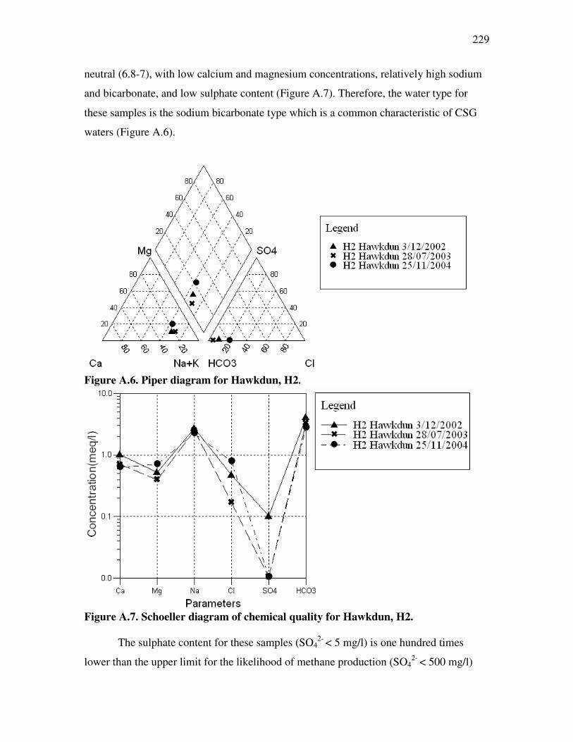
229
neutral (6.8-7), with low calcium and magnesium concentrations, relatively high sodium
and bicarbonate, and low sulphate content (Figure A.7). Therefore, the water type for
these samples is the sodium bicarbonate type which is a common characteristic of CSG
waters (Figure A.6).
Figure A.6. Piper diagram for Hawkdun, H2.
Figure A.7. Schoeller diagram of chemical quality for Hawkdun, H2.
The sulphate content for these samples (SO42- < 5 mg/l) is one hundred times
lower than the upper limit for the likelihood of methane production (SO42- < 500 mg/l)

230
presented by Van Voast (2003). This, along with the relatively high bicarbonate
concentrations (250 mg/l, 202 mg/l, and 170 mg/l) suggests sulphate reduction is taking
place. The methane bearing potential of the Hawkdun lignites was confirmed with CSG
desorption results of core canisters which produced significant quantities of methane gas.
This confirms the assumption that sulphate reduction is taking place within the coal
seams. Alkalinity and bicarbonate levels decrease at about the same rate across the three
samples. This suggests initial bicarbonate concentrations could have been higher for the
first sample because some of this bicarbonate could have originated from the
carbonaceous mudstones overlapping the coal seams within the Manuherikia group. This
could be observed as foam like bubbles when this groundwater first flowed to the surface
(Figure A.8). As vertical flow continued, the mudstones along the edge of the borehole
could have been washed away leaving just the coal seams exposed within the borehole.
The coal seams could have then subsided one on top of the other thus restricting the flow
of water from the carbonaceous units. Therefore, subsequent samples might better
resemble what could be expected from pure CSG waters. The same analysis holds true for
the dissolved carbon dioxide in water samples.
For this borehole, dissolved metals concentrations (arsenic, iron, manganese,
chromium, mercury, and zinc) are low in comparison to what could be expected from an
acid mine drainage situation. This is because there is no oxidation taking place and the
water pH is fairly neutral. Total iron and manganese concentrations are just over the
maximum acceptable values specified in the NZ drinking water standards (0.02 mg/l for
iron and 0.05 mg/l for manganese), but these values are still fairly low in comparison to
waters arising from other operations (i.e. AMD).

231
Figure A.8. Bubbly flow from the H2 borehole on 2/12/2002 (3:30pm).
The three H2 samples plotted in Figure A.6 represent the percentage of major ions
in each of the water samples being analysed. Sample points in this figure do not coincide;
this shows the extent of variations in major ion composition. However, in a situation like
the one in borehole H2, these variations could be expected mainly because the hole is not
cased. Consequently, the hole is subjected to changes in water flow from unconfined
units; therefore, this hole may be subjected to seasonal variations and changes in water
quality.

232
Table A.5. Hawkdun H2 samples Sample date 3/12/2002 28/07/2003 25/11/2004 pH pH units 6.8 7 6.9 Specific Conductance (T=25ºC) µS/cm� 386 342 401 TDS mg/l 309 262 336 Hardness mg/l as CaCO3 76.5 (a) 54.7 (a) 67 Alkalinity mg/l as CaCO3 205 166 140 Bicarbonate (HCO3 -) mg/l 250 (b) 202 (b) 170 (b) Carbonate (CO3
2-) mg/l 0.09 (b) 0.12 (b) 0.08 (b) Carbon dioxide (CO2 (aq)) mg/l 141 (b) 73 (b) 77 (b) Calcium (Ca2+) mg/l 20.2 14 12.8 Magnesium (Mg2+) mg/l 6.32 4.8 8.5 (c) Sodium (Na+) mg/l 62.2 57.3 51.7 (d) Potassium (K+) mg/l 10.4 6 NA Chloride (Cl-) mg/l 16.6 6 28 Sulphate (SO4
2-) mg/l 4.9 <0.5 <2 Zinc (Zn2+) mg/l <0.001 0.04 NA Fluoride (F) mg/l NA 0.38 NA Boron (B) mg/l NA 0.3 NA Silica (SiO2) mg/l NA 58.9 NA Dissolved Organic Carbon mg/l NA 8.8 NA Total Iron (Fe) mg/l NA 3.7 NA Manganese (Mn) mg/l NA 0.29 NA Arsenic (As) mg/l NA <0.02 NA Barium (Ba2+) mg/l NA <0.002 NA Chromium (Cr2+) mg/l NA <0.01 NA Mercury (Hg) mg/l NA <0.002 NA Selenium (Se) mg/l NA <0.02 NA Notes: NA= Not Available. 3/12/2002 sample analysed through Hill Laboratories. 28/07/2003 sample analysed through CRL Energy and Hill laboratories. 25/11/2004 sample analysed at the EEL (University of Canterbury). (a) Calculated from calcium and magnesium concentrations (b) Calculated from carbonate equilibrium using known alkalinity and pH (c) Calculated from known hardness and calcium concentrations (d) Calculated assuming zero electro neutrality and neglecting minor ions. This value also includes K+ ions.

233
A.3 Sample collection methods
Background information
In 2002 CRL Energy Ltd and L&M Mining Ltd applied for research funds for a
PhD, through The University of Canterbury, to the New Zealand Foundation for Research
Science and Technology (FRST). These funds were granted taking the form of a
Technology for Industry Fellowship (TIF) to fund living expenses, enrolment costs, and
some study-related costs associated with this PhD work. Although it was intended that
CRL Energy and L&M Mining would pay all drilling, sampling, and analysis costs of the
research, no funds were made explicitly available to fund the work itself. Instead,
contractual provisions were made by these companies, to meet all programme expenses
for the successful completion of the work. In the long run, this proved to be a
considerable problem. The CRL Energy Ltd manager who devised the project left to
work for a CSG competitor, and L&M Mining Ltd took much longer than anticipated to
choose sites for drilling work investigations. In addition, L&M Mining Ltd were more
interested in assessing the CSG resource than in sampling CSG water, so they
concentrated their efforts on drilling as many holes as possible to assess the quality of
coal and CSG potential, and gave low priority to the collection of CSG water samples.
Consequently, these companies were reluctant to spend money to properly case wells and
acquire high water quality pumps to sample CSG waters from the wells they were drilling.
In addition, they decided they were not going to fund a sampling programme to regularly
collect samples, and they were not going to spend money ensuring high quality data were
collected from field investigations. Instead, they were going to supply these data
themselves when the opportunity presented itself. They did, however, commit to
procuring small funds for simple laboratory analyses, and eventually purchased a multi-
metre to use in site investigations.
At this stage, there was little that could be done from the point of view of
designing a proper sampling collection programme, and the methodology adopted in
carrying out this work had to take into account a considerable degree of uncertainty and
lack of control.

234
Methods
The methods for collecting water samples varied depending on different site
conditions, equipment available, and the person collecting the samples. As mentioned
earlier (background information) there was little control over how this was done, but
some basic provisions were taken to try to ensure good quality samples were collected.
For example, clean sample bottles were ordered from certified laboratories (CRL Energy
Ltd and Hill Laboratories) and, in some instances, specific measurements like pH and
Specific Conductance were monitored to ensure that they remained constant prior to
taking the sample. This was to try to make sure that actual aquifer water (and not stagnant
water) was sampled.
The EEL (University of Canterbury) had limited equipment to analyse water
samples. The basic equipment at this laboratory included pH and conductivity meters,
ovens, HACH spectrophotometers, basic reagents, and laboratory equipment. An ICP or
Atomic Absorption machine was not available at the EEL, so it was not possible to
achieve a high degree of accuracy when analysing water samples. Eventually, a sodium
selective electrode was purchased for the purposes of measuring this ion’s concentration
in CSG water, and provisions were made to analyse some of the samples using Atomic
Absorption equipment at the Chemistry Department (University of Canterbury). It was
not straight forward to use the Chemistry Department each time - university policy forces
its different departments to operate as entirely different entities, thus charging money for
services rendered.
The inadequacies of the methods discussed here are clearly evident to the author
and include: the lack of good quality samples from cased boreholes at different sites,
inadequate well purging prior to sample collection, the lack of sample field blanks to
validate the sampling, and not being able to analyse all of the samples through certified
laboratories. Whenever samples were analysed at the EEL (University of Canterbury),
accuracy was compromised due to lack of resources. For example, chloride and sulphate
were measured using HACH methods (see section A.1), and sodium was measured with a
sodium ion electrode; when this instrument was not available, it was necessary to assume
zero electroneutrality to estimate sodium concentrations. These methods are generally not

235
considered accurate methods for estimating analyte concentrations, but they were used
here due to lack of resources.
Ashers-Waituna, Reefton, and Kaitangata
As described by on-site personnel, water from these boreholes was collected when
“artesian conditions” where encountered while the drilling was taking place. These
“artesian conditions” could have been due to air pumped into the borehole by the drillers
to clear the hole and push water out of the well. It was unfortunate that no further
descriptions accompanied the origin of these samples, so these samples were always
treated with caution as to their origins and future use. In any case, these samples were
analysed to provide a future point of comparison, and to present a case for carrying out
good quality sampling to the mining companies doing the exploration work.
Samples were collected in 1000ml clean plastic bottles supplied by the CRL
Energy Ltd laboratory. The samples were completely filled with water taking care there
were no air gaps when closing their lids; no on-site measurements were taken in this case,
but the samples were sent (via courier or delivered by personnel) in containers packed
with ice. These samples were received at the CRL Energy Ltd offices in Christchurch to
analyse at the EEL within 48 hours of collection, where they were analysed for major
ions composition following the methods specified in section A.1
Hawkdun
In this case, true artesian conditions were encountered when the drill bit penetrated
into the lignite seams of the Manuherikia group on 2/12/2002 (section A.2.4). The well
was left opened with water flowing right to the surface for 24 hours before samples were
collected personally on 3/12/2002. At the time of collection, pH and specific conductance
were measured using a calibrated meter, and these data are presented in Table A.6. The
samples were collected in 1000ml bottles (untreated), 250ml bottles (treated with HNO3),
and 750ml glass bottles to preserve different constituents before analyses were carried out.
Once again, samples were collected whilst taking care not to leave any air gaps inside the
bottle and, in case of bottles containing HNO3, taking care not to spill any of the
treatment solutions. After the drilling investigation was completed, the well was capped
with a closed tap to stop the water flow. On 28/07/2003 this tap was opened to collect a

236
second sample. Groundwater started flowing to the surface after a few minutes of
opening the tap, and it was left running for 45min before collecting the sample. In
addition, while water was flowing to the surface, pH and specific conductance were
monitored approximately every 15min, and these data are presented in Table A.6.
Samples were collected in plastic bottles using the same procedure used on the previous
sampling collection event (3/12/2002). A final sample was collected from this borehole
on 25/11/2004. In this instance, a sample was collected by CRL Energy Ltd personnel in
a 1000ml plastic bottle, but without monitoring pH or specific conductance. The sample
was then couriered to Christchurch where it was analysed at the EEL (University of
Canterbury).
Table A.6. Monitoring of pH and Specific Conductance prior to sample collection. Sample Time pH Specific Conductance(µS/cm) 3/12/2002 13:00 6.96 383 28/7/2003 13:13 6.62 361 28/7/2003 13:30 6.88 357 28/7/2003 13:48 6.94 358 28/7/2003 13:59 6.94 360
Maramarua
When C-1 was first drilled in Maramarua, the uncased borehole was sampled
using a subcontractor (DJ Phelps & Co Ltd) with the aid of a special submersible pump.
This subcontractor collected the samples only after the solution chemistry of the
groundwater being pumped had stabilised using temperature, pH, and conductivity as
indicators. Table A.7 presents the field parameters being monitored at the time of
collecting this first sample on 18/09/2003. The sample was collected in a 500ml untreated
bottle for Organics, a 250ml bottle treated with HNO3 for dissolved metals, a 250ml glass
bottle to test for TPH, a 250ml bottle (sulphuric acid preserved), and a 100ml glass bottle
for TOC. Once this sample was collected it was packed in an ice-box and sent to Hill
Laboratories, where it was analysed.

237
Table A.7. Groundwater sampling record for sample collected on 18/9/2003 (9am) Water level Volume pumped Temperature pH Specific Conductance cm litres °C µS/cm 25 0 NA NA NA NA 20 15.2 7.2 950 NA 20 15.1 7.5 970 NA 40 15.1 7.5 960 NA 20 15.1 7.5 970 NA 40 15.1 7.5 970 NA 40 15.1 7.5 960 NA 20 15.1 7.5 960 NA 40 15.1 7.5 960 NA 20 15.1 7.5 970 NA 40 15.1 7.5 960 NA 40 15.1 7.5 960 1698 40 15.1 7.5 970
After C-1 was re-drilled and cased in 2004, subsequent samples were collected
from this well. Samples were collected in 1000ml (unpreserved) plastic bottles supplied
by the CRL Energy Ltd Laboratory. In a few instances, the samples were collected
personally and on-site measurements were carried out on these occasions (Table A.8).
However, for the most part, the samples were collected by an on-site operator, who
followed basic sample collection methods. Samples were collected after the pump had
been dewatering the well for some time, and care was taken not to leave any air gaps in
the sample bottles. Samples were then packed in containers with ice, and couriered to the
CRL Energy Ltd offices in Christchurch for analyses at the EEL (University of
Canterbury).
Table A.8. Groundwater monitoring prior to sample collection Date and time Water level Temperature Specific
Conductance pH
m °C µS/cm 12/9/2004, 17:22 64.8 19.2 1471 7.72 13/9/2004, 14:16 90.6 19.6 1462 7.79 14/9/2004, 9:30 100 18.3 1478 7.85 Note: These measurements were taken only while monitoring pumped water (after 15 minutes) to ensure that these properties remained constant.

238
On 19/8/2004 a sample was collected by the field operator in 1000ml bottles (untreated),
250ml bottles (treated with HNO3), and 750ml glass bottles. The sample was then packed
in an ice-box and sent to Hill Laboratories for a full analysis.
A.4 References
American Public Health Association., American Water Works Association., and Water
Environment Federation., 1999, Standard methods for the examination of water
and wastewater: Washington, D.C., American Public Health Association, 1
computer optical disc p.
Hach Company., 2003, Water analysis handbook : drinking water, wastewater, seawater,
boiler/cooling water, ultrapure water: Loveland, Colo., Hach, 1268 p.
LFTB Study Group., 1986, South Island Phase II Lignite Site Selection Studies
Programme. Resource definition, geotechnical, hydrology, and mine planning
studies. Hawkdun deposit.: Wellington, N.Z., Liquid Fuels Trust Board.
Nielsen, D., 1990, Practical handbook of ground-water monitoring: Chelsea, MI, Lewis
Publishers, x, 717 p.
Pope, S., 2004a, 2004 Coal Seam Gas Exploration Results: Ashers-Waituna Lignite
Deposit, PEP 38-217, Southland.: Christchurch, CRL Energy Ltd, p. 41.
—, 2004b, Coal Seam Gas Exploration Results: Hawkdun Coalfield, Central Otago,
2002-2004.: Christchurch, CRL Energy Ltd, p. 42.
Russell, L.L., 1976, Chemical aspects of groundwater recharge with wastewaters:
Berkeley, University of California.
Snoeyink, V.L., and Jenkins, D., 1980, Water chemistry: New York, Wiley, xiii, 463 p.
Stumm, W., and Morgan, J.J., 1996, Aquatic chemistry : chemical equilibria and rates in
natural waters: New York, Wiley, xvi, 1022 p.
Van Voast, W.A., 2003, Geochemical signature of formation waters associated with
coalbed methane: Aapg Bulletin, v. 87, p. 667-676.
239
B. Appendix B
B.1 Sodium calculations and corrections
Sodium concentrations were measured through the chemistry department
(University of Canterbury). The analytical method used at this laboratory, was APHA
3500 Na-B which uses an atomic absorption spectrophotometer in the flame emission
mode. Unfortunately, due to budget constraints, not all of the samples were measured like
this. Therefore, the rest of the sodium concentrations, in the rest of the samples, were
measured using a sodium probe or determined from zero electroneutrality. The sodium
probe used at the EEL was a Cole-Parmer Sodium Ion Electrode which, if properly
calibrated, is capable of achieving a ±2% reproducibility. The probe manufacturer
recommends calibrating the probe using standards of similar composition and ionic
strength. Therefore, this probe was calibrated against sample values of known sodium
concentrations (previously determined using method 3500 Na-B).
The atomic absorption method and the sodium probe were not available from the
start of the project, therefore some samples were consumed before they could be analysed.
For these samples, the method of zero electroneutrality was used to calculate sodium
concentrations. In this method, the difference between anions and cations (in meq/l) is
calculated for the samples for which sodium concentrations are known from APHA 3500
Na-B (Eq B.1). The differences should be zero (or close to zero) but, because of
accumulated systematic errors, there is a sizeable difference (��= 52.84 mg/l on average).
The next step is to calculate the difference between anions and cations in the samples for
which sodium concentrations are unknown. These differences include the unknown (the
sodium cation) plus a value associated with the accumulated systematic errors.
Consequently, to obtain an estimate of their sodium concentrations, the previously
calculated difference (52.84 mg/l) is added to their final value (Eq B.2). An example of
this calculation procedure is presented in Table B.1.
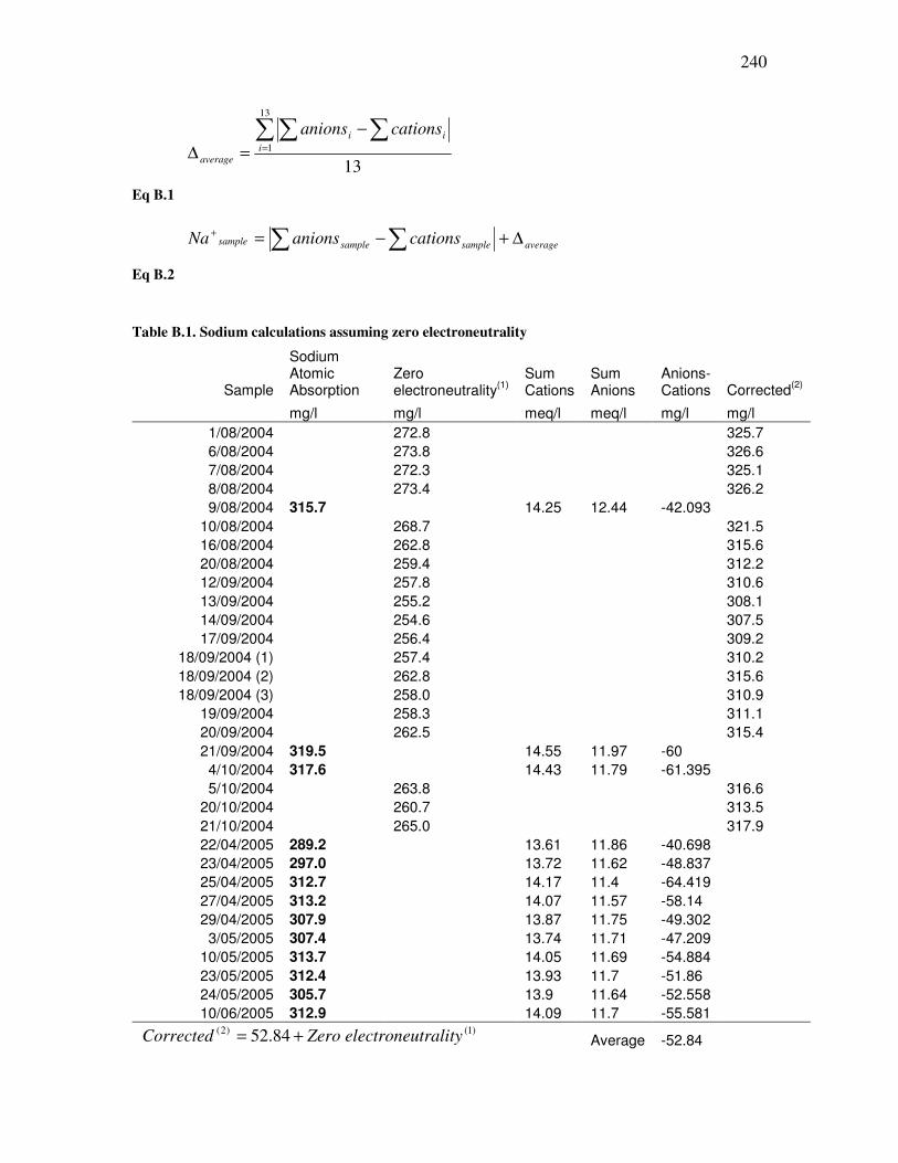
240
13
13
1�� �
=
−=∆ i
ii
average
cationsanions
Eq B.1
averagesamplesamplesample cationsanionsNa ∆+−= � �+
Eq B.2 Table B.1. Sodium calculations assuming zero electroneutrality
Sample
Sodium Atomic Absorption
Zero electroneutrality(1)
Sum Cations
Sum Anions
Anions-Cations Corrected(2)
mg/l mg/l meq/l meq/l mg/l mg/l 1/08/2004 272.8 325.7 6/08/2004 273.8 326.6 7/08/2004 272.3 325.1 8/08/2004 273.4 326.2 9/08/2004 315.7 14.25 12.44 -42.093
10/08/2004 268.7 321.5 16/08/2004 262.8 315.6 20/08/2004 259.4 312.2 12/09/2004 257.8 310.6 13/09/2004 255.2 308.1 14/09/2004 254.6 307.5 17/09/2004 256.4 309.2
18/09/2004 (1) 257.4 310.2 18/09/2004 (2) 262.8 315.6 18/09/2004 (3) 258.0 310.9
19/09/2004 258.3 311.1 20/09/2004 262.5 315.4 21/09/2004 319.5 14.55 11.97 -60 4/10/2004 317.6 14.43 11.79 -61.395 5/10/2004 263.8 316.6
20/10/2004 260.7 313.5 21/10/2004 265.0 317.9 22/04/2005 289.2 13.61 11.86 -40.698 23/04/2005 297.0 13.72 11.62 -48.837 25/04/2005 312.7 14.17 11.4 -64.419 27/04/2005 313.2 14.07 11.57 -58.14 29/04/2005 307.9 13.87 11.75 -49.302 3/05/2005 307.4 13.74 11.71 -47.209
10/05/2005 313.7 14.05 11.69 -54.884 23/05/2005 312.4 13.93 11.7 -51.86 24/05/2005 305.7 13.9 11.64 -52.558 10/06/2005 312.9 14.09 11.7 -55.581
)1()2( 84.52 tralityelectroneuZeroCorrected += Average -52.84

241
B.2 Precision and accuracy
Whenever possible, repetitions were carried out to obtain a true value
(approximated by the average) for the population of measurements being carried out. This
procedure also yields an implicit error (relative standard deviation, standard deviation of
the mean, and relative error) associated with each measured value. Unfortunately, it is not
always possible to carry out many repetitions when sample volumes are limited (see
Appendix G), and CSG waters undergo changes when exposed to normal atmospheric
conditions. Nevertheless, these errors should already be low if the APHA standards are
followed carefully.
pH and Specific Conductance. Meters were calibrated on a regular basis and two
sets of meters were used from time to time to verify their accuracy. In the case of specific
conductance it was found that there is some discrepancy between terminologies that
sometimes leads to confusion among meter users. The term “conductivity” refers to the
ability of a solution to conduct an electric current. This value is measured in µS/cm or
µmho/cm and varies with temperature; it is necessary to define a standard temperature as
a baseline to carry out comparisons. Therefore, the term “specific conductance” has been
defined as the conductivity of a sample measured at 25°C. This value is often expressed
in mS/m, but it can be expressed in any units as long as the property being measured is
adequately specified (in terms of name or temperature). The pH meter used at the EEL
was an EDT Instruments meter model number RE 357, and its accuracy was ±0.02 pH
units (±0.05 with just one significant figure). For specific conductance measurements, a
WTW LF325 Tetracon meter was used, and its accuracy was ±0.5% of the measured
value with a variation of ±1 digit. �
Total Dissolved Solids (TDS). There are three ways of carrying out TDS
measurements. The first one involves drying a sample in an oven at a designated
temperature, and the second one consists of measuring all of the dissolved ions and
calculating the TDS value analytically. The third method, which is an estimate, involves
taking these measurements with a calibrated Specific conductance meter.
Measuring TDS with a meter is not a precise way of determining this parameter
because meters use a basic estimation of TDS based on specific conductance

242
measurements. Eq B.3 presents the relationship relating TDS and specific conductance.
The value of A ranges from 0.54 to 0.96, but usually assumes values between 0.55 and
0.76 depending on the water being analysed (Hounslow, 1995). For the particular case of
the Maramarua CSG samples, A ranged from 0.51 to 0.63.
TDS (mg/l) = A · Specific Conductance (µS/cm) �
Eq B.3 (Hounslow, 1995)
If the value of A is unknown, measuring TDS using a meter would lead to a
considerable degree of uncertainty. Therefore, the TDS values measured at the EEL were
determined by drying a known volume of sample water in an oven following APHA
standards. Again, there seems to be some confusion to the correct application of APHA
standards. APHA specifies different measuring procedures for total solids, total
suspended solids, and total dissolved solids (TDS). It specifies drying temperatures of
103°-105° C for total solids and total suspended solids, but 180°C for TDS. This is
because when the sample is dried up, CO2 and H2O are lost and bicarbonates are
converted to carbonates (Eq B.4). However, at temperatures below 180°C Eq B.4 may
not go to completion, hence APHA specifies a drying temperature of 180°C. This is
particularly important when analysing CSG waters because of the high bicarbonate
content present in these waters. APHA reports on the precision of this procedure by
single-laboratory analyses of 77 samples of a known 293 mg/l TDS concentration which
yielded a standard deviation of differences of 21.20 mg/l.
2HCO3
- � CO32- + CO2 + H2O
Eq B.4 (Hounslow, 1995)
It was discovered that most laboratories around the world are relaxed about the
drying temperature for TDS and often use 103°-105° C instead of 180°C. The EEL is no
exception. This generally would pose no problems in low bicarbonate waters but with
CSG waters overestimation of TDS is definitely a possibility. Therefore, the preferred
temperature used for drying the samples at the EEL was 180° C. Getting the oven to a
temperature of 180° C sometimes was a problem as this lab is shared with other users.
Under these circumstances the samples were originally dried at 103°-105° C; later, when

243
the oven was available, the TDS analyses were repeated but at a temperature of 180°C. It
was discovered that TDS values decreased in 14 out of 19 Maramarua C-1 samples when
using 180°C. The relative differences in the 14 samples which yielded lower results were
about 6% on average and up to 10% in some cases. The remaining 5 samples yielded
higher results possibly due to random errors, but the relative differences were low
anyway (-1.4% on average). Therefore, this comparison provided an important lesson in
terms of determining TDS values in CSG waters.
Another way of determining TDS is by conducting a full ion analysis and then
calculating TDS analytically by adding all the ions plus the silica while taking care of
subtracting the amount of water and carbon dioxide that would be lost in the evaporation
process. Applying stochiometry to Eq B.4, the amount of H2O and CO2 that is lost due to
evaporation is 0.5082· HCO3-. Therefore, this amount needs to be deducted from the sum
of all the ions (including bicarbonate) plus silica contained in solution. In this way, Eq
B.5 presents the relationship for calculating TDS in this fashion. All of these ions and the
silica (SiO2) are expressed in mg/l, so the end result (TDS) also has these units. It was
not possible to calculate TDS values in this way at the EEL because this would have
required a complete ion determination. However, it is important to keep in mind this
calculation procedure as some laboratories do not follow this convention, not
compensating for the amount of carbon dioxide and water that would be lost due to
evaporation (Van Voast, 2003).
TDS (mg/l) = Σ ions (mg/l) + SiO2 (mg/l) – [HCO3- (mg/l)·�0.5082]
�
Eq B.5 (Hounslow, 1995)
Alkalinity. According to APHA, when the alkalinity is due entirely to bicarbonate
and carbonate (10-500 mg/l), a standard deviation of 1 mgCaCO3/L can be achieved, but
an experimental value of 5 mgCaCO3/L is normally obtained (American Public Health
Association. et al., 1999). For the Maramarua analysis, the chosen sample volume was
100ml, and 2-3 repetitions were carried out in 10 of samples. The relative standard
deviation (RSD) for these samples ranged from 0.45% to 3.17%, which is a good
indication of the precision of these results.

244
Hardness. To apply the APHA 2340 C method, a 25ml sample was diluted with
deionised water to 50ml. It was later discovered that this water was not as deionised as
originally thought so these measurements were corrected to take this effect into account;
the analysis was then onwards carried out with 50ml but with no dilution. Consequently,
2-4 repetitions were carried out in 23 of the Maramarua C-1 samples, which produced an
average RSD of 13.46%. This high error percentage is attributed to the difficulties in
measuring low hardness concentration in CSG waters (<33 mgCaCO3/L), and to possible
variations due to calcium carbonate precipitation after the sample is exposed to normal
atmospheric conditions.
Coal Seam Gas waters are subjected to high pressures while in the coal aquifer. At
these pressures the partial pressure of CO2 gas is significantly high (about 0.1 atm),
which allows CO2 gas to stay dissolved in the aquifer water. Once water is pumped up to
the surface, the lower atmospheric pressure causes a lower CO2 partial pressure (about
0.0003 atm). At a lower partial pressure, the dissolved CO2 gas will slowly start to
abandon its dissolved form and will form part of air under normal atmospheric
conditions. This process is not instantaneous and may require anywhere from a few hours
to a few days depending on the degree of agitation and aeration to which the sample is
subjected. As CO2 gas leaves the water samples, the carbonate equilibrium changes in the
samples. Bicarbonate (HCO3-) concentrations decrease in the sample, while carbonate
(CO32-) and pH values increase. As this takes place Ca2+ precipitates as CaCO3, Mg2+
precipitates as dolomite CaMg(CO3)2, and zinc precipitates as smithsonite (ZnCO3) or
hydrozinite Zn5(CO3)2(OH)6. This has direct consequences in the analytical
determination of calcium, magnesium, and zinc ions dissolved in the water sample. If
samples are left for too long they will degas and their chemistry will change. In addition,
there can be a significant differences between repetitions from the same sample
depending on the amount of time that has elapsed between measurements and the degree
of agitation to which each sample has been exposed. However, if precautions are taken,
these effects can be minimized and their importance is only relevant to the time elapsed
since the CSG water has been abstracted from the aquifer and the time of sample
collection. If care is taken not to leave any air gaps in the sample bottle, degassing will be
minimum. However, once the sample bottle is opened, degassing can take place again,

245
but at a very slow rate because the surface tension of the water prevents CO2 gas from
leaving the bottle at once. This process explains the high averaged RSD values (13.46%)
in repetitions taken from hardness measurements of Maramarua samples. A good
approach for solving this problem would be to wait until the sample has been degassed
(or to aerate the sample to accelerate this process) and then measure the dissolved
constituents (after precipitation). This method would produce more stable results but
would ignore the actual concentrations present in the sample before sparging.
Calcium. The precision for this methodology (APHA 3500-Ca A) reported by
APHA yields a RSD of 9.2% and a relative error of 1.9%. As for hardness, calcium
determinations had a similar approach, with some errors being made at the beginning
because 25ml of sample was diluted with 25ml of not-so-deionised water. However, as
with hardness, these measurements were corrected and 50ml of sample volume with no
dilutions were used instead. In this way, 2-5 repetitions were carried out in 23 of the
samples producing an average RSD of 17.32%. Again, this apparently large error is
attributed to the difficulties in measuring small calcium concentrations (<8mg/l) and
CaCO3 precipitation once the sample bottle is opened exposing it to the atmosphere.
Chloride. HACH method 8225 was used to measure chloride. This involves
titrating the sample until there is a colour change from yellow to red-brown. However,
this endpoint is not very clear because while titrating the sample the colour change goes
from yellow to dark orange and finally to red-brown. During this colour sequence, yellow
clusters are present and, as the sample is being stirred, the sample colour seems lighter
than it truly is. Hence, a biased is introduced and a larger amount of titrant than necessary
is added to the sample. However, this error is systematic which means that measurements
carried out using this method can be compared against each other. The HACH manual
does not mention how to correct for this bias or how to calibrate the measuring method
against other systematic errors. Consequently, original chloride measurements where
about 23% greater than the chloride concentration from the sample analysed through the
CRL Energy laboratory (19/8/2004). Therefore, HACH method 8225 was calibrated
against known chloride concentrations. The result of this produced a linear regression
formula (Figure B.1) with an excellent coefficient of determination (R2=0.9957). In this

246
way, chloride measurements where corrected using the linear regression equation
presented in Figure B.1.
Chloride calibration for HACH 8225
y = 0.8844x - 8.5073R2 = 0.9957
0
50
100
150
200
250
0 50 100 150 200 250 300
Measured
Theo
retic
al (a
ctua
l val
ues)
Figure B.1. Calibration of HACH method 8225
On average, chloride concentrations analysed at the EEL were 144 mg/l, while the
value measured at the CRL Energy laboratory (19/8/2004 sample) was 146 mg/l. Since
CRL Energy uses an ion chromatography (APHA 4110 B) this value should be more
precise than the HACH titration method (with calibration). Consequently, the relative
error using HACH is 1.44%. To determine an associated error, 2-5 repetitions were
carried out in 18 on the Maramarua samples being analysed. The average RSD obtained
using this methodology was 1.41%.
HACH method 8225 does not include an estimate of its precision, but it does
provide guidelines to test the accuracy of the additions and solutions. For example, the
standard 0.0141N silver nitrate solution decomposes with light, so it was tested regularly
using a sodium chloride standard solution of 1000mg/l as Cl-.
Sulphate. The HACH 8051 method used for measuring sulphate, works only for
the range of values from 2 to 70 mg/l and uses a digital spectrophotometer device to carry
out the sulphate determination. Its sensitivity is reported within a 1 mg/l of SO42- range
(Hach Company., 2003), and the methodology leaves little room for random errors. In 31
out of the 33 Maramarua C-1 samples analysed using this procedure, sulphate
concentrations were below the detectable range of values (<2 mg/l). This was confirmed

247
with the 19/8/2004 sample analysed at the CRL Energy laboratory which uses ion
chromatography (APHA 4110 B) and which reported a value of 0.7 mg/l.
Carbonate equilibrium. The uncertainty associated with the different carbonate
species was calculated using error propagation techniques as described in Meyer (1975).
For the bicarbonate concentrations of the Maramarua C-1 samples, the average relative
standard deviation (RSD) is 20.4% (9.2% min and 23.8% max); for carbonate, the
average RSD is 18.4% (8.3% min and 21.6% max); for dissolved carbon dioxide the
average RSD was 25.5% (11.5% min and 29.4% max).
Precision and accuracy - discussion
The values for New Zealand CSG water presented in this document correspond to
the average of measurement repetitions performed on collected samples. It was possible
to store some of these samples in sealed bottles to avoid CaCO3 precipitation. However,
after a period of approximately 4 weeks, a white sediment was observed in some of these
bottles. This could have been CaCO3 precipitation which could have been produced if
CO2 gas came out of solution under lower partial pressure conditions (this gas could have
left the bottle through the cap or could have remained trap in an air gap inside the bottle).
Another possibility is that this CaCO3 could have precipitated through a slow diffusion
process. Therefore, it was decided not to use these samples to produce more repetitions
on the measured parameters. This is a valid objection because the error of the mean is
directly proportional to the error of a single observation. Thus, “a reduction by a factor of
10 in the average error of individual measurements produces the same improvement in
the precision of the mean as do 100 repetitions” (Meyer, 1975). Consequently, a calcium
titration performed on a sample in which CaCO3 was allowed to precipitate would
introduce a bias when averaging this value along previous titrations performed on the
sample with no CaCO3 precipitation.
Because there is uncertainty in the analytical methods used, it is necessary to
clarify a few points. First of all, sulphate concentrations for most of the Maramarua (C-1)
2004/2005 samples analysed at the EEL (University of Canterbury) are unknown, but
lower than 2 mg/l (<0.0420 meq/l). Therefore, in order to plot these values in the Piper
and Schoeller diagrams (Chapter 3 - figures 3.6, 3.7, and 3.8), a nominal value of 0.02

248
meq/l was chosen for these samples. Secondly, the methods for calculating magnesium in
these samples could give way to error generation. This is because magnesium is
calculated by measuring hardness and calcium, and then subtracting calcium from
hardness. However, hardness is not only given entirely by magnesium and calcium
because other elements like strontium, barium, and some heavy metals can add to the
hardness of samples (Hounslow, 1995). This can be observed with the full analysis (CRL
Energy laboratory) from the 19/8/2004 which indicated the presence of some heavy
metals and barium; its Schoeller diagram (Chapter 3 – figure 3.8) shows the magnesium
concentration for this sample below the calculated concentrations for 2004 and 2005
samples. However, the main source of errors is given by the combination of errors when
determining both hardness and calcium, which translates into error amplification. For
example, some random errors could have been made when measuring hardness (errors in
judgement, ambient fluctuations, etc.), thereby producing a result which already contains
an associated error. When measuring calcium, a different set of random errors associated
with the calcium values is generated and, when combined with the hardness values, these
yield even wider fluctuations. It is possible to observe graphically (Chapter 3 – figure 3.8)
this phenomenon by inspecting the variations of the 2004/2005 samples measured at the
EEL (University of Canterbury). Here, the variations for these samples are lower for
calcium than for magnesium. The same analysis holds true for sodium values, which have
been calculated in the 2004/2005 samples by assuming zero electro neutrality in the water
samples analysed at the EEL. However, in this case because sodium values are much
higher than calcium or magnesium values, these differences are not noticeable when
taking their logarithm. Hence sodium values appear with practically no variation.

249
B.3 Time plots for parameters
Time plot for Magnesium
0.01.02.03.04.05.06.0
0.00 50.00 100.00 150.00 200.00 250.00 300.00 350.00
days
Mag
nesi
um (m
g/l)
First round Second round
Time plot for pH
7.0
7.2
7.4
7.6
7.8
8.0
0.00 50.00 100.00 150.00 200.00 250.00 300.00 350.00
days
pH
First round Second round
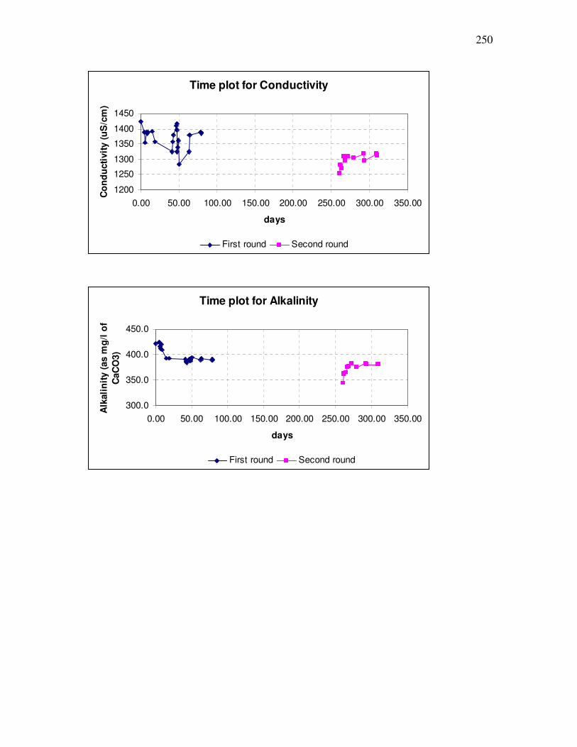
250
Time plot for Conductivity
1200
1250
1300
1350
1400
1450
0.00 50.00 100.00 150.00 200.00 250.00 300.00 350.00
days
Con
duct
ivity
(uS
/cm
)
First round Second round
Time plot for Alkalinity
300.0
350.0
400.0
450.0
0.00 50.00 100.00 150.00 200.00 250.00 300.00 350.00
days
Alk
alin
ity (a
s m
g/l o
f C
aCO
3)
First round Second round

251
Time plot for Hardness
0.010.020.030.040.050.060.0
0.00 50.00 100.00 150.00 200.00 250.00 300.00 350.00
days
Har
dnes
s (a
s m
g/l o
f C
aCO
3)
First round Second round
Time plot for Carbonate
0.00
1.00
2.00
3.00
4.00
0.00 50.00 100.00 150.00 200.00 250.00 300.00 350.00
days
Car
bona
te (m
g/l)
First round Second round
Time plot for H2CO3*
0.0
20.0
40.060.0
80.0
100.0
0.00 50.00 100.00 150.00 200.00 250.00 300.00 350.00
days
H2C
O3* (m
g/l)
First round Second round
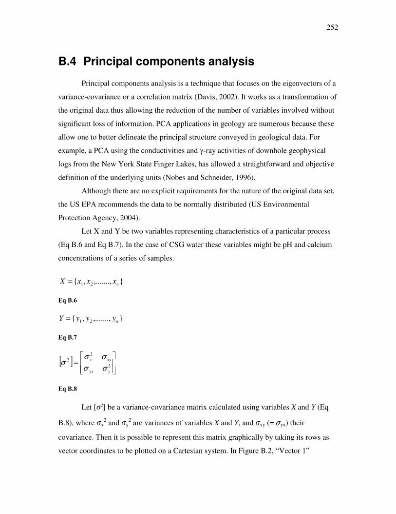
252
B.4 Principal components analysis
Principal components analysis is a technique that focuses on the eigenvectors of a
variance-covariance or a correlation matrix (Davis, 2002). It works as a transformation of
the original data thus allowing the reduction of the number of variables involved without
significant loss of information. PCA applications in geology are numerous because these
allow one to better delineate the principal structure conveyed in geological data. For
example, a PCA using the conductivities and �-ray activities of downhole geophysical
logs from the New York State Finger Lakes, has allowed a straightforward and objective
definition of the underlying units (Nobes and Schneider, 1996).�
Although there are no explicit requirements for the nature of the original data set,
the US EPA recommends the data to be normally distributed (US Environmental
Protection Agency, 2004).
Let X and Y be two variables representing characteristics of a particular process
(Eq B.6 and Eq B.7). In the case of CSG water these variables might be pH and calcium
concentrations of a series of samples.
},.......,,{ 21 nxxxX =
Eq B.6
},.......,,{ 21 nyyyY =
Eq B.7
[ ]���
�
���
�= 2
22
yyx
xyx
σσσσ
σ
Eq B.8
Let [�2] be a variance-covariance matrix calculated using variables X and Y (Eq
B.8), where �x2 and �y
2 are variances of variables X and Y, and �xy (= �yx) their
covariance. Then it is possible to represent this matrix graphically by taking its rows as
vector coordinates to be plotted on a Cartesian system. In Figure B.2, “Vector 1”

253
represents the first row of matrix [�2], while “Vector 2” represents its second row. The
eigenvectors of [�2] will have the same slope as the principal axes (I and II) of the ellipse
in Figure B.2; the eigenvalues (�I and �II) represent the length of its principal semi axes. It
is important to note that the eigenvectors of [�2] are mutually orthogonal, and the sum of
its eigenvalues is equal to the sum of the elements in its diagonal (�x2 + �y
2) with each
variable making its own contribution to the total variance.
The sum of the principal semi axes’ length represent the total variance associated
with [�2], but their individual lengths correspond to the calculated eigenvalues and not to
the individual variances. Therefore, each eigenvalue contributes to the total variance,
however the proportion at which this takes place is different to the contribution of
individual variances. This time the major principal semi axis (I) will be responsible for
most of the variance, while the secondary principal semi axis (II) will only account for a
small contribution.
Figure B.2. Graphic representation of a variance-covariance matrix.

254
It is possible to project the original set of data on to the principal semi axis (I and
II) through a transformation defined by a linear combination of eigenvalues. Let A be the
matrix of eigenvalues of [�2], and AI and AII matrix vectors of A (Eq B.9). If �1 and �2 are
the components of AI, and �1 and �2 are the components of AII, then the transformation of
the original data set, X and Y, into the principal component space, XZ and YZ, will be of
the form presented in Eq B.10. This transformation is presented in matrix notation in Eq
B.11.��
[ ] ��
���
���
���
���
���
�==
2
1
2
1
ββ
αα
III AAA
Eq B.9
21111 αα ⋅+⋅= yxXZ 21111 ββ ⋅+⋅= yxYZ
22122 αα ⋅+⋅= yxXZ 22122 ββ ⋅+⋅= yxYZ . . . . . .
21 αα ⋅+⋅= nnn yxXZ 21 ββ ⋅+⋅= nnn yxYZ Eq B.10. Principal components space transformations
[ ] [ ] [ ][ ] AYX
yx
yx
yx
YZXZZ
nn
⋅=��
���
�⋅
��������
�
�
��������
�
�
⋅⋅⋅⋅⋅⋅
==22
11
22
11
βαβα
Eq B.11
The new data set, Z, is referred to as the “principal components scores” or simply
“scores”, whereas the matrix of eigenvalues, A, is referred to as the “principal
components loadings” or “loadings”(Davis, 2002). The scores, XZ and YZ, will be
uncorrelated because the principal semi axes on to which these are projected are mutually
orthogonal. What's more, the variance of the first new data set, XZ, will be equal to the
first eigenvalue, and the variance of the second new data set, YZ, will be equal to the
second one. Thus, the new data sets will contain the same total variance as the original

255
data set, but the partial distribution of variance will fall on each separate data set, XZ or
YZ, which will be equal to their corresponding eigenvalues.
The analysis can be extended to more than just two sets of variables, so a large
number of properties or characteristics can be included; plotting the scores on principal
components space becomes complicated and sometimes impossible but the validity of the
analysis still holds. In theory, there is no restriction regarding the minimum number of
observations to carry out a principal components analysis. However, variances and
covariances need a large sample size before stabilising, and for 2 or less observations (n ��
2) it is not possible to calculate these values. To deal with incommensurate units, it is
possible to standardize the original data by subtracting the average and dividing by the
standard deviation for each data point. In this case, the variance-covariance matrix
becomes the correlation matrix, [R], and the PCA is carried out using the latter. A straight
forward way of computing the correlation matrix is by transposing the original data set
and multiplying it by itself, the result is then divided by n-1 to avoid bias (Eq B.12). In
this case, the diagonal of [R] will contain ones, and the sum of these will be equal to the
number of vector columns (properties or characteristics). �
][][1
1][ GG
nR t ⋅
−=
where [G] is a matrix containing the original data set in vector columns n is the total number of samples or observations Eq B.12
The analysis of principal components usually focuses on analysing the effect that
each variable (property or characteristic) has on the total variation. In addition, the
analysis can solely focus on those eigenvectors whose eigenvalues account for the
majority of the variance, which simplifies the problem. By concentrating on analysing the
loadings it is possible to determine which characteristics are relevant within each
eigenvector. This process sometimes is referred to as “reification”(Davis, 2002). If the
studied phenomenon has several characteristics (in the case of CSG water these could be
pH, calcium concentration, alkalinity, etc.) then a PCA could determine which of these
characteristics is responsible for the most variation in the data set. Furthermore, a closer

256
examination of the loadings responsible for the highest contribution of variance can
provide important information about the processes involved in shaping this variation.
PCA is a powerful technique; however it is not straightforward because it works by
interpreting the transformed data and its components, and not the actual data set. Also, in
PCA the number of principal components (eigenvalues of A) is always equal to the
number of variables, which can complicate the scrutiny of results if there are too many
variables or if their eigenvalues are similar in magnitude. A different variation of PCA,
factor analysis, deals with these issues and proves quite effective in describing the
processes involved.
B.5 Factor analysis
Given a [G]nxm data matrix, the objective of factor analysis is to select p-variates
from a total of m-variates, and to express the data matrix of p-variates into common
factors (common to all the p variables) and unique factors (unique to each of the p
variables) (Haan, 1977). This decomposition can be expressed using algebraic notation
for each of the n rows of matrix [G]nxm , in the following way:
mp
mjfaG j
p
rrjrj
<
=+⋅=�=
.....11
ε
Eq B.13 (Davis, 2002).
In Eq B.13, ajr are the factor loading coefficients, fr, are the common factors, and
�j are the unique factors representing the random variation unique to Gj. Common
applications of factor analysis in hydrology, however, are normally carried out by
ignoring the unique factors, �j (Matalas and Reiher, 1967; Wallis, 1967).
To simplify the analysis, it is possible to express the factor loading coefficients
and the common factors in matrix notation. In this way, [AR] will be an mxp matrix of
factor loadings and [F] will be an nxp matrix of common factors. The different values of
Gj are assumed to be multivariate and normally distributed. Therefore the
variance/covariance matrix can be calculated by multiplying [AR] by its transpose and

257
then adding the independent variations (Eq B.14) (Davis, 2002). If the unique factors are
ignored, Eq B.14 can be further simplified. Also, if the data are standardised using Eq
B.12, then the variance/covariance matrix becomes the correlation coefficient matrix, [R].
[ ] [ ] [ ] [ ]jj
tRR AA εσ var2 +⋅= Eq B.14 (Davis, 2002).
The analysis then focuses not on calculating the actual factor decomposition of Gj,
but rather on calculating the loading matrix, [AR], and the matrix of factor scores, [SR]. As
in the case of PCA, the analysis of the factor loading matrix can provide insight in
determining the most relevant processes involved in shaping a particular data set.
However, this time the analysis focuses on analysing the loadings of an actual factor
decomposition rather than a factor transformation.
Before outlining the Factor Analysis procedure, it is necessary to consider the
number of factors to be extracted. Originally, there are m number of variates, and the
challenge is to extract a fewer number (p) of these without significant loss of information.
Determining the number of factors to be extracted is not straight forward and requires
some subjectivity. The simplest strategy for selecting the number of factors to be
extracted, is to decide on the value of p before carrying out the analysis (Davis, 2002).
This can be done if there is some hint on the number of possible factors for a particular
problem. Some researchers recommend extracting only two or three factors because this
is the maximum number of factors that can be displayed on a diagram (Davis, 2002).
Another approach in selecting the number of factors to be extracted is to select only those
factors that are responsible for most of the variance, which is reflected by the
corresponding eigenvalues. For example, an “elbow” in a scree plot (a plot of the
eigenvalues against their corresponding factor numbers) shows the maximum number of
factors to extract (UCLA Academic Technology Services). Figure B.3 shows an example
of such an elbow configuration in a scree plot - in this case only 8 factors should be
extracted.
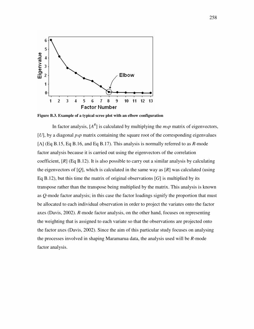
258
Figure B.3. Example of a typical scree plot with an elbow configuration
In factor analysis, [AR] is calculated by multiplying the mxp matrix of eigenvectors,
[U], by a diagonal pxp matrix containing the square root of the corresponding eigenvalues
[Λ] (Eq B.15, Eq B.16, and Eq B.17). This analysis is normally referred to as R-mode
factor analysis because it is carried out using the eigenvectors of the correlation
coefficient, [R] (Eq B.12). It is also possible to carry out a similar analysis by calculating
the eigenvectors of [Q], which is calculated in the same way as [R] was calculated (using
Eq B.12), but this time the matrix of original observations [G] is multiplied by its
transpose rather than the transpose being multiplied by the matrix. This analysis is known
as Q-mode factor analysis; in this case the factor loadings signify the proportion that must
be allocated to each individual observation in order to project the variates onto the factor
axes (Davis, 2002). R-mode factor analysis, on the other hand, focuses on representing
the weighting that is assigned to each variate so that the observations are projected onto
the factor axes (Davis, 2002). Since the aim of this particular study focuses on analysing
the processes involved in shaping Maramarua data, the analysis used will be R-mode
factor analysis. �
�

259
mxpmmm
U
������
�
�
������
�
�
⋅⋅⋅⋅⋅⋅⋅⋅⋅⋅⋅⋅⋅⋅⋅⋅⋅
⋅⋅
=
ψβα
ψβα 111
][
where, the columns of [U] are the eigenvectors of [�2] or [R]
Eq B.15
[ ] [ ] [ ]t
p
I λ
λ
λλ
⋅=
������
�
�
������
�
�
⋅⋅=Λ
00000000000000000000
2
1
where, ��= p eigenvalues of [�2] or [R] [I] = pxp identity matrix�
Eq B.16
[ ] [ ] [ ]
������
�
�
������
�
�
⋅⋅⋅⋅⋅⋅⋅⋅⋅⋅⋅⋅⋅⋅⋅⋅⋅⋅⋅⋅⋅
⋅⋅⋅
=Λ⋅=
mpm
p
R
aa
a
aaa
UA
1
21
11211
Eq B.17 The factor loadings in Eq B.17 have the same direction as the eigenvectors and
their magnitudes are given by the square roots of their eigenvalues. For example, if just
the first two factors are selected (first two columns of matrix [AR] in Eq B.17) and m=2
then the two factors can be represented in a two dimensional coordinate system (Figure
B.4). Here, the first two factors are orthogonal and their coordinates are given by their
corresponding factor loadings (in vector columns); their magnitudes are in fact the square
roots of their eigenvectors. In this way, the eigenvalues represent the proportion of the
total variance accounted for by the eigenvectors. The sums of the squared factor loading
coefficients for each row of the matrix in Eq B.17 are referred to as “communalities”, and
these represent the amount of each variable’s variance retained throughout the factors. If
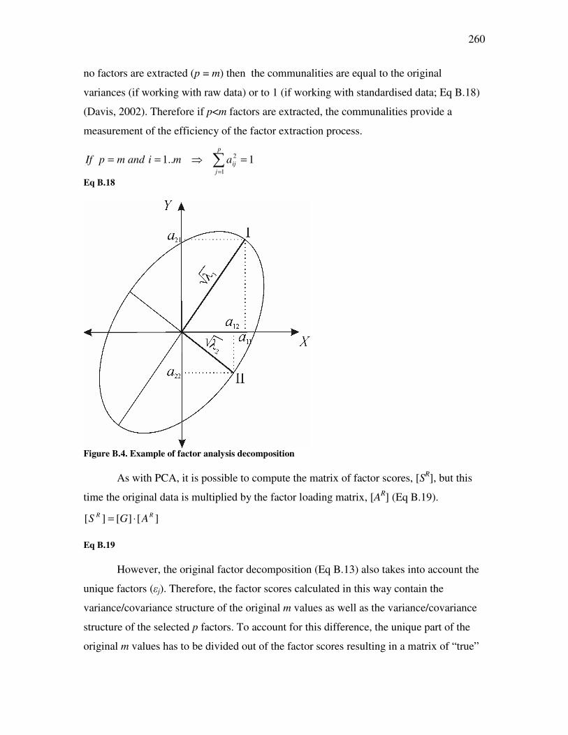
260
no factors are extracted (p = m) then the communalities are equal to the original
variances (if working with raw data) or to 1 (if working with standardised data; Eq B.18)
(Davis, 2002). Therefore if p<m factors are extracted, the communalities provide a
measurement of the efficiency of the factor extraction process.
1..11
2 =�== �=
p
jijamiandmpIf
Eq B.18
Figure B.4. Example of factor analysis decomposition
As with PCA, it is possible to compute the matrix of factor scores, [SR], but this
time the original data is multiplied by the factor loading matrix, [AR] (Eq B.19).
][][][ RR AGS ⋅= Eq B.19
However, the original factor decomposition (Eq B.13) also takes into account the
unique factors (�j). Therefore, the factor scores calculated in this way contain the
variance/covariance structure of the original m values as well as the variance/covariance
structure of the selected p factors. To account for this difference, the unique part of the
original m values has to be divided out of the factor scores resulting in a matrix of “true”

261
factor scores (Davis, 2002). This is done by pre multiplying the factor loadings by the
inverse of the variance/covariance matrix [�2] or correlation matrix [R] (Eq B.20). The
matrix of factor score coefficients, [B], is defined by Eq B.21 further simplifying Eq B.20
into Eq B.22.
][][][][ 1 RRTrue ARGS ⋅⋅= −
Eq B.20
][][][ 1 RARB ⋅= − Eq B.21
][][][ BGS RTrue ⋅=
Eq B.22
In this way, the analysis of the matrix of factor score coefficients, [B], allows
determining the variates with the highest influence, and the possible interrelationships or
processes involved in shaping the data. In addition, a plot of the scores could provide
insight into the influence of selected factors on selected properties inherent to the original
data set. Consequently, a factor analysis transformation can be a powerful tool when
determining which processes have the highest impact on a final outcome shaping a
particular data set. Sometimes, however, it is not possible to determine which factors
have the highest or lowest impacts as these appear to have very similar weights. In these
instances, it is possible to force the analysis into exaggerating these differences thus
making it easier to interpret factor analyses results.
The factor loading matrix contains the correlations between the loadings and the
original variables. Therefore, the factors plot in axes that are orthogonal to each other in p
space. There are, however, m-p axes that have been removed, and it is possible to further
rotate the remaining p axes. Such a procedure is normally referred to as “factor rotation”.
There are several rotation techniques, but the most popular one is the “varimax” scheme
first defined by Kaiser (1958). In this technique, the factor axes are rotated so that the
projection of each loading onto the axes is either near the origin or far away from it.
Therefore, the factor loading matrix is rotated by multiplying it to an orthogonal matrix,
[T] (Eq B.23), so that the correlations between the loadings and the original variables is
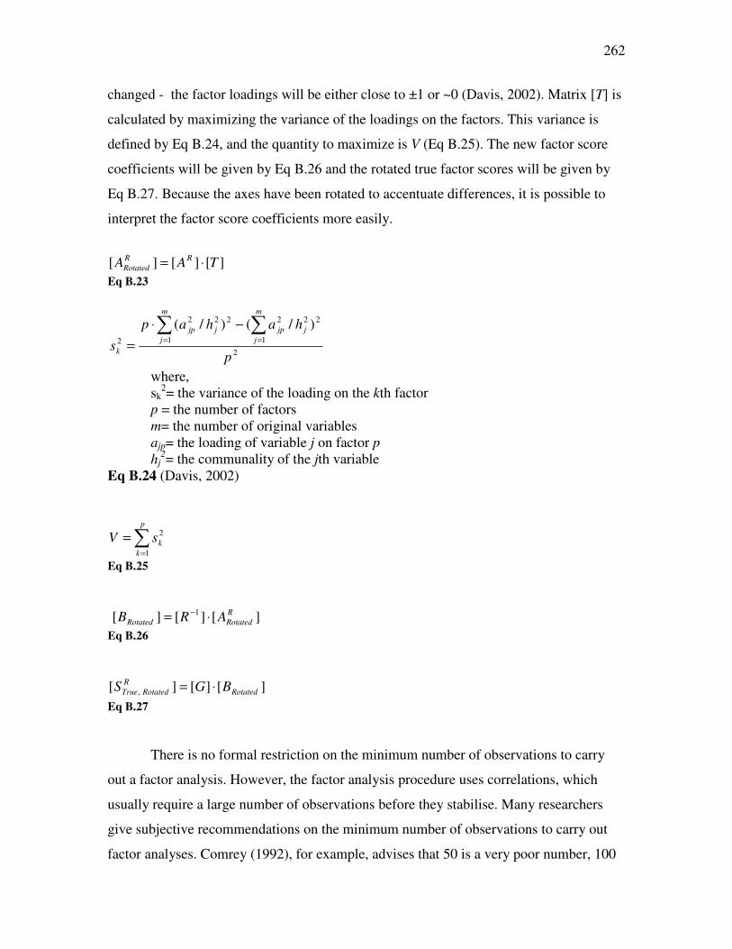
262
changed - the factor loadings will be either close to ±1 or ~0 (Davis, 2002). Matrix [T] is
calculated by maximizing the variance of the loadings on the factors. This variance is
defined by Eq B.24, and the quantity to maximize is V (Eq B.25). The new factor score
coefficients will be given by Eq B.26 and the rotated true factor scores will be given by
Eq B.27. Because the axes have been rotated to accentuate differences, it is possible to
interpret the factor score coefficients more easily.�
][][][ TAA RR
Rotated ⋅= Eq B.23
2
1 1
222222
2
)/()/(
p
hahaps
m
j
m
jjjpjjp
k
� �= =
−⋅=
where, sk
2= the variance of the loading on the kth factor p = the number of factors m= the number of original variables ajp= the loading of variable j on factor p hj
2= the communality of the jth variable Eq B.24 (Davis, 2002)
�=
=p
kksV
1
2
Eq B.25 ][][][ 1 R
RotatedRotated ARB ⋅= − Eq B.26
][][][ , RotatedR
RotatedTrue BGS ⋅= Eq B.27
There is no formal restriction on the minimum number of observations to carry
out a factor analysis. However, the factor analysis procedure uses correlations, which
usually require a large number of observations before they stabilise. Many researchers
give subjective recommendations on the minimum number of observations to carry out
factor analyses. Comrey (1992), for example, advises that 50 is a very poor number, 100

263
is poor, 200 is fair, 300 is good, 500 is very good, and 1000 or more is excellent. Hatcher
(1994) recommends that the number of observations should be either five times the
number of variables or 100, whichever is larger. On the other hand, Bryant and Yarnold
(1995) recommend that the ratio between number of observations and variables should be
5 or larger. During CSG exploration, these recommendations are hard to implement
simply because the number of samples is always limited. Therefore additional
precautions have to be taken when dealing with a small number of observations. For
example, the data can be checked for outliers and tested for normality prior to carrying
out the analysis. Also, once the factor analysis is carried out, it should be checked that the
communalities are close to 1.
B.6 Implementing Factor Analysis using MINITAB
MINITAB is a computer program designed to carry out advanced statistical
calculations. It was originally developed in 1972 by faculty members of The
Pennsylvania State University to aid in the teaching of statistics at university level. The
main feature in MINITAB is its user-friendliness and versatility- this program is now
established as a bench mark program in statistical analysis, and is used in a variety of
applications including research, industry, and science. The latest release is version 14,
and its features include regression analysis, analysis of variance, reliability/survival
analysis, time-series and forecasting, and multivariate analysis to mention a few
(MINITAB Inc, 2005). The multivariate analysis techniques in MINITAB include PCA
and Factor Analysis. However, the calculation procedure is not explained in the software
manuals, and the technical language is verbal rather than mathematical which can become
confusing at times. For example, the terms “scores” and “coefficients” are loosely used in
MINITAB indistinctly on whether the analysis being carried out is PCA or Factor
Analysis. The correct terminology would be to use the terms “principal component
scores” and “principal component loadings” when carrying out PCA, and to use the terms
“factor scores” and “factor score coefficients” when performing a factor analysis.
However, once the user gets used to this terminology PCA and Factor Analyses are easy
to implement and the user can focus his or her attention in interpreting results rather than

264
on performing tedious calculations. Therefore, the analysis of Maramarua CSG water
quality data was carried out using MINITAB v14. Prior to carrying out the analysis it was
necessary to test the data for normality and, in cases where the data did not follow a
normal distribution, transformations were duly applied. MINITAB does not require a
predefined number of observations to carry out factor analyses. However, it does require
more observations than variables to carry out the calculations.
B.7 Data transformation for factor analysis
The test of normality used in this analysis was the W test developed by Shapiro
and Wilk(1965). This procedure tests the H0 null hypothesis “the population has a normal
distribution” versus the HA hypothesis “the population does not have a normal
distribution”. To do this, the two most extreme values are subtracted and multiplied by a
constant (this constant reflects the tendency of extreme values in normal distributions
(Milke and Huitric, 1993)). This process is carried out with subsequent extreme values,
and the final result (W) is then summed, squared, and divided by the sum of the squared
deviations of the original data set. The W value is then compared against a known W�
value which has been developed by Shapiro and Wilk(1965) using Monte Carlo
simulations. If W<W� ,the null hypothesis (H0) is rejected and HA is accepted. In this test,
the significance level (�) reflects the probability of inadvertently rejecting the null
hypothesis when it is in fact true. Therefore, small values of � are more conservative than
larger ones; for this analysis, a 1% significance level (99% confidence) was employed to
select a W� value for testing the null hypothesis. If the null hypothesis was false using this
significance level (HA), then a transformation was applied to the data set so that the
hypothesis was not false anymore (H0). The transformations used for this purpose were
selected using the MINITAB software which is able to calculate the optimal
transformation to normalise data that do not follow a normal distribution. Table B.2
shows the normalised parameters and their selected transformations (if any) passing the
W test, and the original data vs. the transformed data are plotted in figures 5-7.

265
Table B.2. Normalised parameters and their selected transformations (if any) after W test (�=0.1%) Parameter Transformation Mean/transformed
mean Std. dev./ transformed std. dev.
pH NTR 7.7 0.18 TDS NTR 773 24.13 Alkalinity x
½� 19.8 0.37
Hardness NTR 26.7 4.03 Calcium NTR 5.6 1.03
Chloride ��
���
�
−−⋅+
xx
Log63.159
48.13918.18.1 1.04 0.42
Carbonate NTR 1.72 0.66 Carbon dioxide ��
���
� −⋅+−75.5
90.23asinh03.118.1
x -0.03 1.08
Sodium NTR 314.1 5.71 Water column NTR 101.86 42.65 NTR = No transformation required
330.0340.0350.0360.0370.0380.0390.0400.0410.0420.0430.0
1 2 3 4 5 6 7 8 9 10 11 12 13 14 15 16 17 18 19 20 21 22 23 24 25 26 27 28 29 30 31
samples
Alk
alin
ity
18.0
18.5
19.0
19.5
20.0
20.5
21.0
Tran
sfor
med
alk
alin
ity
Alkalinity Transformed Alkalinity
Figure B.5. Original alkalinity data plotted against transformed alkalinity data

266
134136138140142144146148150152
1 2 3 4 5 6 7 8 9 10 11 12 13 14 15 16 17 18 19 20 21 22 23 24 25 26 27 28 29 30 31
samples
Chl
orid
e
0.0
0.5
1.0
1.5
2.0
2.5
Tran
sfor
med
chl
orid
e
Chloride Transformed Chloride
Figure B.6. Original chloride data plotted against transformed chloride data
0.010.020.030.040.050.060.070.080.090.0
100.0
1 2 3 4 5 6 7 8 9 1011 12 1314 15 1617 1819 20 2122 23 2425 26 2728 29 3031
Car
bon
diox
ide
-2.5-2.0-1.5-1.0-0.50.00.51.01.52.02.5
Tran
sfor
med
car
bon
diox
ide
Carbon dioxide Transformed carbon dioxide
Figure B.7. Original carbon dioxide data plotted against transformed carbon dioxide data.
267
B.8 References
American Public Health Association., American Water Works Association., and Water
Environment Federation., 1999, Standard methods for the examination of water
and wastewater: [Washington, D.C.], American Public Health Association, 1
computer optical disc p.
Bryant, F.B., and Yarnold, P.R., 1995, Principal components analysis: Thousand Oaks,
CA, Sage Publications.
Comrey, A.L., and Lee, H.B., 1992, A first course in factor analysis: Hillsdale, N.J., L.
Erlbaum Associates, xii, 430 p.
Davis, J.C., 2002, Statistics and data analysis in geology: New York, J. Wiley, xvi, 638 p.
Haan, C.T., 1977, Statistical methods in hydrology: Ames, Iowa State University Press,
xv, 378 p.
Hach Company., 2003, Water analysis handbook : drinking water, wastewater, seawater,
boiler/cooling water, ultrapure water: Loveland, Colo., Hach, 1268 p.
Hatcher, L., 1994, A step-by-step approach to using the SAS system for factor analysis
and structural equation modeling: Cary, N.C., SAS Institute, xiv, 588 p.
Hounslow, A., 1995, Water quality data : analysis and interpretation: Boca Raton, Lewis
Publishers, 397 p.
Kaiser, H.F., 1958, The Varimax Criterion for Analytic Rotation in Factor-Analysis:
Psychometrika, v. 23, p. 187-200.
Matalas, N.C., and Reiher, B.J., 1967, Some Comments on Use of Factor Analyses:
Water Resources Research, v. 3, p. 213-&.
Meyer, S.L., 1975, Data analysis for scientists and engineers: N.Y., Wiley, 513 illus. p.

268
Milke, M.W., and Huitric, R.L., 1993, Simulating Errors in Statistical Tests of Leachate-
Impacted Groundwater Quality: Ground Water, v. 31, p. 645-653.
MINITAB Inc, 2005, MINITAB, Volume 2005: Pennsylvania.
Nobes, D.C., and Schneider, G.W., 1996, Results of downhole geophysical measurements
and vertical seismic profile from the Canandaigua borehole of New York State
Finger Lakes: Special Paper - Geological Society of America, v. 311, p. 51-63.
Shapiro, S.S., and Wilk, M.B., 1965, An Analysis of Variance Test for Normality
(Complete Samples): Biometrika, v. 52, p. 591-&.
US Environmental Protection Agency, 2004, Statistical Primer, Volume 2005, p. web
page.
UCLA Academic Technology Services, Factor Analysis Using SAS PROC FACTOR, in
Services, U.A.T., ed., Volume 2005: Los Angeles, p. Web page.
Van Voast, W.A., 2003, Geochemical signature of formation waters associated with
coalbed methane: Aapg Bulletin, v. 87, p. 667-676.
Wallis, J.R., 1967, When Is It Safe to Extend a Prediction Equation - an Answer Based
Upon Factor and Discriminant Function Analysis: Water Resources Research, v. 3,
p. 375-&.
269
C. Appendix C
C.1 Infiltration risk model
Introduction
Discharge of high-SAR water, such as CSG water, on to the land can result in soil
infiltration problems resulting from soil dispersion and loss of aggregation. The
parameters that influence the chemical dispersion phenomenon are: soil salinity, sodicity
(ESP), clay content, organic matter content, cation exchange capacity (CEC), and soil
drainage.
Materials and Methods
A GIS study using ArcMap was carried out using the Fundamental Soil Data
Layer (FSDL) obtained from Landcare Research New Zealand Ltd (Landcare Research
New Zealand Ltd, 2000). This database contains information on CEC, soiltype, salinity,
organic matter, and drainage for New Zealand soils. The soiltype included references to
the soils’ main texture type, but this information had to be summarized into broader
categories (clay, sand, loam, sand, silt, and gravels) to determine clay percentage (which
plays an important role in assessing soil dispersion).
CEC and clay content were considered to be properties which contribute to soil
dispersion potential, while salinity, organic matter, and drainage were assumed to be
attenuating properties. All of these properties, but soiltype, were already subdivided into
5 categories in the FSDL, however some of these had to be reclassified so that the scoring
system was consistent throughout (1-5 with 1 the best score and 5 the worst). As
previously mentioned, soiltype was rearranged into main texture format, and a scoring
system which reflected the clay percentage was developed - a score of 3 was assigned to
clay, 2 to loam, 1 to silt, -2 to peat, and 0 to everything else. These scores, along with the
class scores for the rest of the properties being analysed, were added or subtracted to

270
produce an Infiltration Problem Potential (IPP) index (Table C.1 and Eq C.1). This results
in a model for assessing infiltration potential problems from the soil point of view. That
is, this model aims at assessing soil response to prolonged leaching with high SAR water,
for example, but assuming that this exposure will take place in the long term. Therefore,
rainfall or potential evapotranspiration will not influence the final result, which is
unavoidable in the long-term.
Table C.1. Salinity categories used in IPP model CEC class Salinity Texture (Clay %) Organic
matter C Drainage
1: very low 1: very low -2: peat 1: very low 1: very poor 2: low 2: low 0: sand and gravels 2: low 2: poor 3: medium 3: medium 1 silt (up to 25%
clay) 3: medium 3: imperfect
4: high 4: high 2: loam 4: high 4: moderately well 5: very high 5: very high 3: clay 5: very high 5: well
5.145.0 +⋅−−−+= DrainagematterOrganicclassSalinityclassTextureclassCECIPPEq C.1
All of the scores, which are added or subtracted in Eq C.1, are weighted in the
same manner except for drainage. Drainage was assigned a weight of 0.5 because this
value was derived from in situ visual interpretations of the soil profile, while the rest of
the values were obtained using analytical techniques. It is important to note that some
terms (salinity, organic matter, and drainage) in Eq C.1 are being subtracted from the IPP.
This is because these properties can actually enhance soil permeability. For example,
salinity can provide aggregation and soil stability (Oster, 1979), and adequate drainage
helps maintain good soil stability. Similarly, organic matter can provide bonding agents
which helps maintain good soil structure (Cameron, 2003). A value of 14.5 is added to
the final IPP value to avoid negative values which could arise when dealing with soils
with low CEC, low clay percentage, high peat content, high salinity, high organic matter,
and high drainage. The final model was calibrated assuming Central Otago (Allen et al.,
1998) soils would have serious infiltration problems (alkali soils), and soils from

271
Clandeboye (Cameron et al., 2003) would have moderate infiltration problems when
irrigated with high-SAR water.
Results
All of the properties affecting soil infiltration under high-SAR irrigation regimes
were plotted in various graphs with their different categories. CEC class and Organic
Matter content have already been presented in Chapter 3 (Ch. 3: Figures 1 and 2), and
salinity class, texture class, and drainage class plots are presented in Figures 1, 2, and 3 in
this appendix. However, the main result of this analysis is the IPP index classification as
presented in Figure 3 (Chapter 3). This figures’ analysis has been presented in Chapter 3.
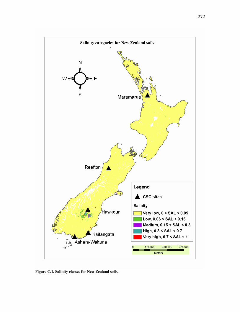
272
Figure C.1. Salinity classes for New Zealand soils.

273
Figure C.2. Main soil texture distribution for New Zealand soils.

274
Figure C.3. Drainage classes for New Zealand soils.

275
C.2 Soil Salinity calculations
Soil salinity assessment calculations were carried out in accordance to the salinity
model presented in the ANZECC guidelines. Water quality (EC, SAR) and soil properties
(clay%, CEC, and ESP) were considered along with rainfall and irrigation to calculate the
relevant leaching fraction. Once this was done, an average root zone salinity was
calculated, and this gave an indication of the crop tolerance and plant response for a
given salinity. The model is presented as follows:
Leaching fraction under rain fed conditions The leaching fraction (LF) is the proportion of water leaching below the root zone, and
this is an essential parameter used for the estimation of salinity and infiltration problems.
The basis of this approach is a salt mass balance approach after equilibrium conditions
are reached. Consequently, the LF can be estimated by calculating the ratio between input
salinity (rainfall) and output salinity (drainage).
%)100/(
)100/(Clay
gmmolcCECgmmolcCCR =
Eq C.2. From ANZECC (2000) where,
CCR = Clay mineralogy which is expressed in mmolc/100g
CEC = Cation exchange capacity expressed in mmolc/100g
Clay % = number from 1-100 expressing the percentage of clay in relation to sand and loam materials
Note: 1 mmolc/100g is equivalent to 1 meq/100g, but mmolc is used here to be consistent with ANZECC
guidelines notation.
The electrical conductivity of the soil saturation extract (ECSE) is then calculated using
the rainfall depth, soil ESP, and parameters depending on the soil CCR.
��
� ⋅⋅+
= ESPDEC
ba
SE
rr
EClog
10 Eq C.3 (Shaw, 1996, as cited in ANZECC and ARMCANZ 2000) .

276
where,
ECr = the electrical conductivity of rain which is assumed to be 0.03 dS/m
Dr = rainfall depth in mm/year for the area being analysed.
ESP is the Exchangeable sodium percentage of the soil calculated using Eq C.4 where
both Na and CEC are in meq/100g
Parameters a and b are obtained from Table 9.2.8 in the ANZECC guidelines(2000) using
soil CCR and Clay %
100][ ×=
CECNa
ESP
Eq C.4 It is now possible to calculate the leaching fraction (LFr) under rain-fed conditions:
SE
rr EC
ECLF
⋅=
2.2
Eq C.5 (Shaw, 1996, as cited in ANZECC and ARMCANZ 2000). where 2.2*ECSE is an estimative value for the electrical conductivity of the drainage
water below the root zone (ANZECC, 2000).
This LFr is the amount of water draining below the root zone under rain-fed conditions,
and it is an indication of soil infiltration as affected by salinity. However, in this case
rainfall has low salinity. In the next section a similar analysis is explained, but this time
the water used in this assessment has high salinity.
Land application (irrigation) of CSG waters When irrigating with high-SAR values, over prolonged periods of time, ESP values will
increase and thus need to be adjusted. This adjustment uses the SAR of the water and a
relationship between ESP and SAR, which was developed from soil samples taken from
9 western states in the US (US Salinity Laboratory Staff, 1954).
)01475.00126.0(1)01475.00126.0(100
d
d
SARSAR
ESP⋅+−+⋅+−⋅
=
Eq C.6 (US Salinity Laboratory Staff, 1954)

277
Where the SARd value is the adjusted SAR value which accounts for calcium carbonate
precipitation. The SARd value is calculated using the RNa procedure formulated by
Suarez (Suarez, 1981, as cited in Ayers and Westcot 1985).
To assess the salinity hazard prior to irrigating with CSG waters of known quality,
it is necessary to calculate the leaching fraction with the corrected ESP values. For this
purpose, the electrical conductivity (ECi) of the irrigation water needs to be calculated
while considering rain or other sources (surface waters for example).
���
�
���
�−⋅⋅= 35.165.2
r
irf EC
ECLFLF
Eq C.7 (ANZECC and ARMCANZ, 2000) where,
LFr = leaching fraction under rain-fed conditions (Eq C.5)
ECi = Weighted EC of input water from irritation and rainfall in dS/m
Eq C.7 must be applied with care. In the case of leaching under rain-fed
conditions (with no ESP correction) this value often exceeds 100%. However, by
definition, the leaching fraction cannot exceed 100%, so when calculation of LFr
produces a result larger 100% the leaching fraction would correspond to the maximum
(100%).
The average root zone leaching fraction is then calculated using the following
relationship:
( ) 625.0022.0976.0 +⋅= fav LFLF
Eq C.8 (Rhoades, 1982 and Shaw et al., 1987, as cited in ANZECC and ARMCANZ 2000) The predicted root zone salinity is then calculated using the following relationship:
av
iSE LF
ECEC
⋅=
2.2
Eq C.9 (Shaw, 1996, as cited in ANZECC and ARMCANZ 2000).
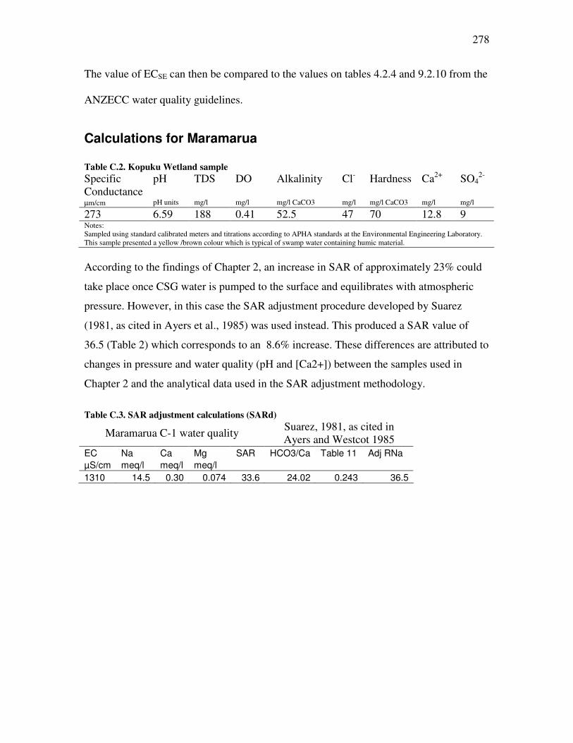
278
The value of ECSE can then be compared to the values on tables 4.2.4 and 9.2.10 from the
ANZECC water quality guidelines.
Calculations for Maramarua Table C.2. Kopuku Wetland sample Specific Conductance
pH TDS DO Alkalinity Cl- Hardness Ca2+ SO42-
µm/cm� pH units mg/l mg/l mg/l CaCO3 mg/l mg/l CaCO3 mg/l mg/l
273 6.59 188 0.41 52.5 47 70 12.8 9 Notes: Sampled using standard calibrated meters and titrations according to APHA standards at the Environmental Engineering Laboratory. This sample presented a yellow /brown colour which is typical of swamp water containing humic material. According to the findings of Chapter 2, an increase in SAR of approximately 23% could
take place once CSG water is pumped to the surface and equilibrates with atmospheric
pressure. However, in this case the SAR adjustment procedure developed by Suarez
(1981, as cited in Ayers et al., 1985) was used instead. This produced a SAR value of
36.5 (Table 2) which corresponds to an 8.6% increase. These differences are attributed to
changes in pressure and water quality (pH and [Ca2+]) between the samples used in
Chapter 2 and the analytical data used in the SAR adjustment methodology.
Table C.3. SAR adjustment calculations (SARd)
Maramarua C-1 water quality Suarez, 1981, as cited in Ayers and Westcot 1985
EC Na Ca Mg SAR HCO3/Ca Table 11 Adj RNa µS/cm meq/l meq/l meq/l 1310 14.5 0.30 0.074 33.6 24.02 0.243 36.5

279
Table C.4. Clay %, CCR, and a and b parameters calculations
Sample Pit Depth pH Specific Conductance CEC Na ESP Clay CCR
Table 9.2.8 ANZECC guid.
# mm µS/cm meq/100g meq/100g % % meq/100g a b 1 1 0-150 5.5 79.9 10 0.12 1.20% 16 0.63 0.44 -0.934 2 1 150-450 5.1 76 10 0.14 1.40% 24 0.42 0.33 -0.857 3 2 0-150 5.6 34 13 0.17 1.31% 13 1.00 -0.559 -0.067 4 2 150-450 5.1 57.7 11 0.21 1.91% 28 0.39 0.411 -0.936 5 3 0-150 6.1 41.9 14 0.08 0.57% 27 0.52 0.411 -0.936 6 3 150-450 5.1 36.6 7 0.025 0.36% 32 0.22 0.147 -0.672 Note: Rainfall from closest weather station (Maramarua Forest, 1947-1980) is 1263 mm/year
Table C.5. Land disposal with 100% CSG water Long term effects Without ESP correction Long term effects with ESP correction
leaching under irrigation Leaching under rain fed conditions
leaching under rain-fed
Prediction Long-term
Long term effects with ESP correction rain
irrig water sa
mpl
e
Pit ECSE LFr ECi LFf LFav ECSE SAR ESP ECSE LFr ECi LFf LFav ECSE # # dS/m % dS/m dS/m % dS/m % dS/m % % dS/m 1 1 0.110 12.4% 1.31 100% 99.9% 0.60 36.5 34.5% 2.5 0.5% 1.31 9% 24.8% 2.4 2 1 0.127 10.8% 1.31 100% 99.9% 0.60 36.5 34.5% 2.0 0.7% 1.31 11% 28.1% 2.1 3 2 0.220 6.2% 1.31 100% 99.9% 0.60 36.5 34.5% 0.3 5.0% 1.31 80% 87.4% 0.7 4 2 0.157 8.7% 1.31 100% 99.9% 0.60 36.5 34.5% 2.4 0.6% 1.31 9% 25.6% 2.3 5 3 0.051 26.8% 1.31 100% 99.9% 0.60 36.5 34.5% 2.4 0.6% 1.31 9% 25.6% 2.3 6 3 0.061 22.3% 1.31 100% 99.9% 0.60 36.5 34.5% 1.3 1.0% 1.31 17% 34.9% 1.7

280
Table C.6. Crop salinity assessment with 100% CSG water
Plant salt tolerance groupings. Criteria based on ECSE and Table 4.2.4 from ANZECC (2000) EXAMPLES
Ayers and Westcot (1985)
Sam
ple
Pit Sensitive crops
Moderately sensitive crops
Moderately tolerant crops
Tolerant crops
Very tolerant crops
Generally too saline
White Clover (NZ) Sensitive
Barley, forage Very tolerant
Salinity assessed on the basis of EC of irrigation water
# # Very low Low Medium High Very High Extreme Yield Yield Degree of restriction on use
1 1 Low yield Low yield 100% yield 100% yield 100% yield 100% yield 86% 100% Slight to moderate 2 1 Low yield Low yield 100% yield 100% yield 100% yield 100% yield 89% 100% Slight to moderate 3 2 100% yield 100% yield 100% yield 100% yield 100% yield 100% yield 100% 100% Slight to moderate 4 2 Low yield Low yield 100% yield 100% yield 100% yield 100% yield 87% 100% Slight to moderate 5 3 Low yield Low yield 100% yield 100% yield 100% yield 100% yield 87% 100% Slight to moderate 6 3 Low yield 100% yield 100% yield 100% yield 100% yield 100% yield 93% 100% Slight to moderate Table C.7. Land disposal with 70% CSG water and 30% rain water
Long term effects without ESP correction Long term effects with ESP correction Leaching under rain-fed leaching under irrigation Leaching under rain fed conditions
Prediction Long-term
Long term effects with ESP correction rain
irrig water
Sam
ple
Pit ECSE LFr ECi LFf LFav ECSE SAR ESP ECSE LFr ECi LFf LFav ECSE # # dS/m % dS/m dS/m % dS/m % dS/m % % dS/m 1 1 0.110 12.4% 0.93 99.9% 100% 0.42 25.5 26.7% 2.0 0.7% 0.93 9% 25.4% 1.7 2 1 0.127 10.8% 0.93 99.9% 100% 0.42 25.5 26.7% 1.6 0.9% 0.93 12% 28.5% 1.5 3 2 0.220 6.2% 0.93 83% 89% 0.47 25.5 26.7% 0.3 5.1% 0.93 68% 78.7% 0.5 4 2 0.157 8.7% 0.93 99.9% 100% 0.42 25.5 26.7% 1.9 0.7% 0.93 10% 26.3% 1.6 5 3 0.051 26.8% 0.93 99.9% 100% 0.42 25.5 26.7% 1.9 0.7% 0.93 10% 26.3% 1.6 6 3 0.061 22.3% 0.93 99.9% 100% 0.42 25.5 26.7% 1.1 1.2% 0.93 16% 34.5% 1.2
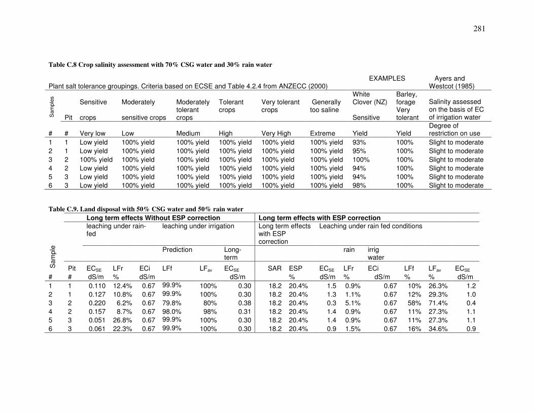
281
Table C.8 Crop salinity assessment with 70% CSG water and 30% rain water
Table C.9. Land disposal with 50% CSG water and 50% rain water
Long term effects Without ESP correction Long term effects with ESP correction
leaching under rain-fed
leaching under irrigation Long term effects with ESP correction
Leaching under rain fed conditions
Prediction Long-
term rain irrig
water
Sam
ple
Pit ECSE LFr ECi LFf LFav ECSE SAR ESP ECSE LFr ECi LFf LFav ECSE # # dS/m % dS/m dS/m % dS/m % dS/m % % dS/m 1 1 0.110 12.4% 0.67 99.9% 100% 0.30 18.2 20.4% 1.5 0.9% 0.67 10% 26.3% 1.2 2 1 0.127 10.8% 0.67 99.9% 100% 0.30 18.2 20.4% 1.3 1.1% 0.67 12% 29.3% 1.0 3 2 0.220 6.2% 0.67 79.8% 80% 0.38 18.2 20.4% 0.3 5.1% 0.67 58% 71.4% 0.4 4 2 0.157 8.7% 0.67 98.0% 98% 0.31 18.2 20.4% 1.4 0.9% 0.67 11% 27.3% 1.1 5 3 0.051 26.8% 0.67 99.9% 100% 0.30 18.2 20.4% 1.4 0.9% 0.67 11% 27.3% 1.1 6 3 0.061 22.3% 0.67 99.9% 100% 0.30 18.2 20.4% 0.9 1.5% 0.67 16% 34.6% 0.9
Plant salt tolerance groupings. Criteria based on ECSE and Table 4.2.4 from ANZECC (2000) EXAMPLES
Ayers and Westcot (1985)
Sensitive Moderately Moderately Tolerant Very tolerant Generally White Clover (NZ)
Barley, forage
Sam
ples
Pit crops sensitive crops tolerant crops
crops
crops
too saline Sensitive
Very tolerant
Salinity assessed on the basis of EC of irrigation water
# # Very low Low Medium High Very High Extreme Yield Yield Degree of restriction on use
1 1 Low yield 100% yield 100% yield 100% yield 100% yield 100% yield 93% 100% Slight to moderate 2 1 Low yield 100% yield 100% yield 100% yield 100% yield 100% yield 95% 100% Slight to moderate 3 2 100% yield 100% yield 100% yield 100% yield 100% yield 100% yield 100% 100% Slight to moderate 4 2 Low yield 100% yield 100% yield 100% yield 100% yield 100% yield 94% 100% Slight to moderate 5 3 Low yield 100% yield 100% yield 100% yield 100% yield 100% yield 94% 100% Slight to moderate 6 3 Low yield 100% yield 100% yield 100% yield 100% yield 100% yield 98% 100% Slight to moderate

282
Table C.10. Crop salinity assessment with 50% CSG water and 50% rain water
Plant salt tolerance groupings. Criteria based on ECSE and Table 4.2.4 from ANZECC (2000)
EXAMPLES
Ayers and Westcot (1985)
White Clover (NZ)
Barley, forage
Sam
ple
Pit
Sensitive crops
Moderately sensitive crops
Moderately tolerant crops
Tolerant crops
Very tolerant crops
Generally too saline Sensitive Very
tolerant
Salinity assessed on the basis of EC of irrigation water
# # Very low Low Medium High Very High Extreme Yield Yield Degree of restriction on use
1 1 Low yield 100% yield 100% yield 100% yield 100% yield 100% yield 98% 100% None 2 1 Low yield 100% yield 100% yield 100% yield 100% yield 100% yield 100% 100% None 3 2 100% yield 100% yield 100% yield 100% yield 100% yield 100% yield 100% 100% None 4 2 Low yield 100% yield 100% yield 100% yield 100% yield 100% yield 99% 100% None 5 3 Low yield 100% yield 100% yield 100% yield 100% yield 100% yield 99% 100% None 6 3 100% yield 100% yield 100% yield 100% yield 100% yield 100% yield 100% 100% None

283
Table C.11. Comparison of leaching fractions with or without ESP correction.
No ESP correction With ESP correction
Sample Pit LFr LFav LF Increase LFr LFav LF Increase # # % % % % % 1 1 12.4% 99.9% 87.4% 0.5% 24.8% 24.2% 2 1 10.8% 99.9% 89.1% 0.7% 28.1% 27.4% 3 2 6.2% 99.9% 93.7% 5.0% 87.4% 82.4% 4 2 8.7% 99.9% 91.2% 0.6% 25.6% 25.1% 5 3 26.8% 99.9% 73.0% 0.6% 25.6% 25.1% 6 3 22.3% 99.9% 77.5% 1.0% 34.9% 33.8% 1 1 12.4% 99.9% 87.4% 0.7% 25.4% 24.7% 2 1 10.8% 99.9% 89.1% 0.9% 28.5% 27.7% 3 2 6.2% 89.0% 82.8% 5.1% 78.7% 73.7% 4 2 8.7% 99.9% 91.2% 0.7% 26.3% 25.5% 5 3 26.8% 99.9% 73.0% 0.7% 26.3% 25.5% 6 3 22.3% 99.9% 77.5% 1.2% 34.5% 33.3% 1 1 12.4% 99.9% 87.4% 0.9% 26.3% 25.4% 2 1 10.8% 99.9% 89.1% 1.1% 29.3% 28.2% 3 2 6.2% 79.8% 73.6% 5.1% 71.4% 66.3% 4 2 8.7% 98.0% 89.3% 0.9% 27.3% 26.3% 5 3 26.8% 99.9% 73.0% 0.9% 27.3% 26.3% 6 3 22.3% 99.9% 77.5% 1.5% 34.6% 33.1%
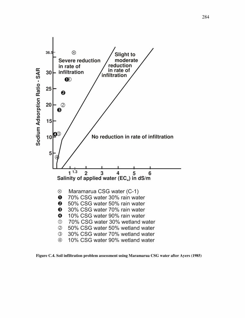
284
�
�
��
��
�
1 2 3 4 5 6
5
10
15
20
25
30
36.5
Salinity of applied water (EC ) in dS/mw
Sod
ium
Ads
orpt
ion
Rat
io -
SA
R
No reduction in rate of infiltration
Slight to moderate
reductionin rate of
infiltration
Severe reductionin rate ofinfiltration
1.3
⊗
Figure C.4. Soil infiltration problem assessment using Maramarua CSG water after Ayers (1985)

285
Table C.12. Crop tolerance to sodium and chloride toxicity associated with Maramarua CSG water Ion CSG Water
mg/l Sensitive Moderately
sensitive Moderately tolerant
Tolerant
Chloride 146 OK OK OK OK Sodium 334 Not OK Not OK May be OK OK
Notes: CSG water from Maramarua C-1 (19/8/2004 sample, see Chapter 1) Sensitive crops: almond, apricot, citrus, plum, grape Moderately sensitive: pepper, potato, tomato Moderately tolerant: barley, maize, cucumber, lucerne, safflower, sesame, sorghum Tolerant: cauliflower, cotton, sugar beet, sunflower

286
C.3 References
Allen, R.B., McIntosh, P.D., and Wilson, J.B., 1998, The distribution of plants in relation
to pH and salinity on inland saline/alkaline soils in Central Otago, New Zealand.
(vol 35, pg 517, 1997): New Zealand Journal of Botany, v. 36, p. 153-153.
ANZECC, and ARMCANZ, 2000, Australian and New Zealand Guidelines for Fresh and
Marine Water Quality, ACT: Australian and New Zealand Environmental and
Conservation Council (ANZECC),
Agricultural and Resource Management Council of Australia and New Zealand
(ARMCANZ): Canberra.
Ayers, R.S., Westcot, D.W., and Food and Agriculture Organization of the United
Nations., 1985, Water quality for agriculture: Rome, Food and Agriculture
Organization of the United Nations, xii, 174 p.
Cameron, K.C., Di, H.J., Anwar, M.R., Russell, J.M., and Barnett, J.W., 2003, The
"critical" ESP value: does it change with land application of dairy factory
effluent?: New Zealand Journal of Agricultural Research, v. 46, p. 147-154.
Landcare Research New Zealand Ltd, 2000, The New Zealand National Soils Database
Spatial Extension, Soil Fundamental Data Layers: Lincoln, Landcare Research
New Zealand Ltd.
Rhoades, J.D., 1982, Reclamation and management of salt-affected soils after drainage.
In Rationalisation of water
and soil research and management, Proceedings of the First Annual Western Provincial
Conference: Lethbridge, Canada, p. 123–197.
Shaw, R.J., 1996, A unified soil property and sodicity model of salt leaching and water
movement [PhD thesis], University of Queensland.
Shaw, R.J., Thorburn, P.J., and Dowling, A.J., 1987, Principles of landscape, soil and
water salinity: Processes and management options, Proceedings of Brisbane
Region Salinity
Workshop: Part A, in Landscape, soil and water salinity: Brisbane, Queensland
Department of Primary Industries.

287
Suarez, D.L., 1981, Relationship between pHc and sodium adsorption ratio (SAR) and an
alternative method of
estimating SAR of soil or drainage waters: Soil Science Society of America Journal, v. 45,
p. 469-475.
US Salinity Laboratory Staff, 1954, Diagnosis and improvement of saline and alkali soils:
[Washington,, US Govt. Print. Off.], vii, 160 p. p.

288
D. Appendix D
D.1 Description and calculation of separation factor
The reaction between the zeolite material and a concentrated solution (i.e. Na+) can be described using the following relationship(Amphlett, 1964):
ions) containing material zeolite the(i.e. exchange after the phase solid theis
)or ,, containingsolution the(i.e. place taken has exchange after the phase liquid theis
s)experiment through flowin solution feed (i.e.solution edconcentrat orginalor phase liquid theis
)or , , (i.e. cations occluded contains which material zeoliteor material phase solid theis
,
22
22
++
++++
++
++++
++++ +⇔+
NaB
CaMgKA
NaB
KMgCaA
Where
BABA
Then, the equilibrium constant governing this ion exchange reaction can be defined as:
{ } { }{ } { }
[ ] [ ][ ] [ ] B
A
A
B
BABA
BABA
Kγγ
×ΓΓ
×⋅⋅=
⋅⋅= ++
++
++
++
(Amphlett, 1964)
where the symbols { } denote activity, [ ] concentration, Γs are the individual ion activity coefficients in the solid phase, and γs are the activity coefficients for the liquid phase. Then it is possible to define the separation factor r as:
[ ] [ ][ ] [ ]
[ ] [ ][ ] [ ]
zeolitesinionstotalQsolutioninionconcentratoriginalc
BqBc
ycc
xAqAc
Where
xyyx
yxyx
cc
cc
cqqc
BABA
r
o
AB
AA
o
AAAA
AA
AA
AB
BA
A
o
B
B
o
A
BA
BA
====
====
−⋅−⋅=
⋅⋅=
⋅
⋅=
⋅⋅=
⋅⋅=
++
++
++
++
,
)1()1(
(Perry et al., 1973)

289
It is possible to work with one section of the isotherm (fractional) and define the separation factor in terms of the fractional isotherm:
zeolite e within thions ofquantity final solutionin ion concentrat final
zeolite e within thions ofquantity initial solutionin ion concentrat initial the'
,''''''''
===
=
−−=
−−=
q''
c''
q'
c
Whereqqqq
Y
cccc
X
Then the separation factor for the fractional isotherm is defined as:
)1()1(
AA
AA
XYYX
R−⋅−⋅
=
(Perry et al., 1973)

290
D.2 Batch absortion experiment results Phase I. Table D.1. Effect of particle size on ion exchange processes using Ngakuru zeolites (first experiment)
Wwet Wdry Moisture
Zeolite weight
NaCl 1M pH
Spec. Cond. (T=25°C) Calcium Calcium Hardness
g g % g ml mS/cm mg/l as CaCO3 mg/l
mg/l as CaCO3
Passing 150 µm 3.7 3.6 3.1% 1.0074 50 5.5 85.9 235 94 NA 150 µm 3.5 3.3 4.4% 1.0026 50 5.6 85.3 224 89.6 300 300 µm 7.8 7.5 4.0% 1.0016 50 5.4 84.2 196 78 250 600 µm 13.4 12.8 4.5% 1.0019 50 5.1 85.4 196 78 275 1180 µm 25.3 24.3 3.9% 1.0048 50 5.4 86 248 99 320 2360 µm 1.3 1.3 3.4% 1.0013 50 5.3 85.7 248 99 330 Kitty litter 27.1 25.6 5.3% 1.0051 50 4.5 85.9 115 46 NA Notes: Original solution concentration : NaCl 1M Original pH = 7.2 Original specific conductance = 85.7 mS/cm Shanking time: 1 hour 45 min Table D.2. Effect of particle size on ion exchange processes using Ngakuru zeolites (second experiment)
Zeolite weight NaCl 1M pH
Cond (T=25°C) Calcium Calcium Hardness Mg
g ml mS/cm mg/l as CaCO3 mg/l mg/l as CaCO3 mg/l
Passing 150 µm 1.0032 53 5.1 75 248 99.2 315 16 150 µm 1.0019 53 5.4 76.2 244 97.6 320 19 300 µm 1.0026 53 5.4 76.4 236 94 295 14 600 µm 1.0013 53 5.4 76.5 248 99 315 16 1180 µm 1.0034 53 5.4 76.4 264 106 340 19 2360 µm 1.0009 53 5.7 76.7 309 124 NA Notes: Original solution concentration : NaCl 1M Original pH = 6.3 Original specific conductance = 75.4 mS/cm Shanking time: 8 hours

291
Phase II. Table D.3. Experiments to determine dissolution potential of Ngakuru zeolites
Zeolite mass
Vol. pHi pHf SPi SPf Ca Ca Hardness Mg
g ml �S/cm �S/cm mg/l CaCO3 mg/l mg/l CaCO3 mg/l NaCl 0.005M
2.0059 100 6.2 5.5 538 546 20 8 32 3
Deionised Water
1.0031 53 ~7 6.4 1.9 41.8 8 3.2 4.17 NA
Notes: 9.5 hours shaking time Zeolite particle size: 1180 µm pHi = initial pH pHf = final pH Spi =initial Specific Conductance @ T=25°C Spf = final Specific Conductance @ T=25°C
Phase III. Table D.4. Effect on solution characteristics on ion exchange processes using Ngakuru zeolites Solution type
concentration weight zeolites
initial pH
final pH
calcium magnesium absorbed sodium
M g meq/g meq/g meq/g NaCl 1 2.0018 7.20 5.51 0.21 0.79 0.915 NaCl 0.1 2.0018 7.65 6.46 0.14 0.38 0.267 NaCl 0.01 2.0045 7.30 6.39 0.03 0.18 0.096 NaOH 0.01 2.0006 11.52 10.81 0.00 0.00 0.227 Notes:
1) Selected volume was 0.12 litres in all cases 2) Zeolite particle size was 600 µm
Phase IV. Experiment n°2
After 4 service/regeneration cycles the zeolites were still absorbing sodium ions
(21.6 meq/100g in n°9), however there was a 65.4% reduction in mass. In this case, the
first service run showed that the cations originally contained within the zeolite are
calcium, magnesium, and potassium. Hydrogen ions, however, were absorbed during this
first service run (pH increase from 6.34 to 7.47), but in subsequent runs these ions were
released. The first service run yielded a natural sodium exchange capacity of 10.4
meq/100g, but this value tended to increase after each regeneration run, reaching a
292
maximum of 21.6 meq/100g in the last service run. Overall, the exchange process took
place with very small charge balance differences (~0 meq/100g; Table D.5).
Throughout the course of this experiment, the zeolites kept releasing occluded
calcium, magnesium, and potassium cations. Runs n°1-n°3 show calcium cations being
released, but it is not possible to determine where the calcium cations are coming from in
subsequent runs because of regeneration with a strong CaCl2 solution in run n°4.
Similarly, magnesium cations kept being released throughout, but sometimes their release
was undetected (n° 5, 7, and 9).
Due to budget constraints, it was not possible to measure potassium throughout.
However, run n°1 indicated 0.6 meq/l of potassium cations originally in the zeolites, and
potassium was released in run n° 5 (0.07 meq/l). The last run (n°9) resulted in high
potassium levels, but this is due to previous regeneration with KCl.

293
Table D.5. Experiment n°2. Batch sorption experiments with 600µm zeolites
n° Reaction type
zeolite weight
sample volume
Sol. type
initial pH
final pH
final Na+
final Ca2+
final Mg2+
final K+
trapped cations
released cations
charge balance
main cation exchange
g litres meq/l meq/l meq/l meq/l meq/l meq/l meq/l meq/100g 1 Service 4.02 0.225 0.01M
NaCl 6.34 7.47 8.1 0.52 0.28 0.60 1.9 1.4 0.5 10.4
2 Regeneration 2.72 0.125 1M HCl
0.25 0.25 7.7 2.4 0.40 NA 10.5 10.5 0.0 35.4
3 Service 2.08 0.125 0.01M NaCl
6.34 2.81 6.5 0.16 0.08 NA 3.5 1.96 1.5 21.1
4 Regeneration 1.88 0.125 0.09M CaCl2
5.32 5.32 0.7 173.7 6.00 0.00 2.0 6.8 4.8 4.9
5 Service 1.76 0.125 0.01M NaCl
6.34 3.13 8.0 0.32 0.00 0.07 2.0 1.21 0.8 14.1
6 Regeneration 1.66 0.125 0.01M CaCl2
6.62 4.60 0.4 17.9 0.28 NA 2.1 0.67 1.5 2.7
7 Service 1.56 0.125 0.01M NaCl
6.34 3.53 8.6 0.30 0.00 NA 1.4 0.63 0.7 11.0
8 Regeneration 1.45 0.125 0.1M KCl
6.76 3.32 3.5 0.40 0.20 NA NA 4.80 4.8 30.4
9 Service 1.39 0.125 0.01M NaCl
6.34 5.67 7.6 0.20 0.00 2.23 2.4 2.43 0.0 21.6
Notes: 1. NA = not available 2. main cation exchange = meq of main cation intervening in the exchange reaction per 100g of zeolites

294
Experiment n°3 – 5
Table D.6. Batch absorption experiments with 1180µm zeolites n° Reaction
type zeolite weight
sample volume
Sol. type
initial pH
final pH
final Na+
final Ca2+
final Mg2+
final K+
TC RC CB main cation exchange
g litres meq/l meq/l meq/l meq/l meq/l meq/l meq/l meq/100g 1 Service 2.04 0.125 0.01M
NaCl 6.34 6.48 7.3 0.56 0.3 0.51 2.7 1.39 1.3 16.7
2 Regeneration 1.21 0.125 0.09M CaCl2
5.32 5.61 3.2 175.6 0.0 NA NA 3.2 NA 33.0
3 Service 0.96 0.125 0.01M NaCl
6.34 6.91 7.7 0.8 0.0 0.28 2.3 1.07 1.2 29.7
4 Regeneration 0.79 0.125 0.01M CaCl2
6.62 6.45 0.6 17.8 0.0 NA 2.0 0.6 NA 9.3
5 Service 0.65 0.125 0.01M NaCl
6.34 6.27 8.2 0.54 0.0 NA 1.8 0.54 NA 34.3
6 Regeneration 0.55 0.125 0.1M KCl
6.76 6.67 2.1 1.7 0.1 NA 0.0 2.2 NA 47.1
Notes: 1. NA = not available 2. main cation exchange = meq of main cation intervening in the exchange reaction per 100g of zeolites 3. TC = trapped cations; RC = released cations; CB = charge balance

295
Table D.7. Batch absorption experiments with 1180µm zeolites
n° Reaction type
zeolite weight
sample volume
Sol. type
initial pH
final pH
final Na+
final Ca2+
final Mg2+
final K+
TC RC CB main cation exchange
g litres meq/l meq/l meq/l meq/l meq/l meq/l meq/l meq/100g 1 Service 2.00 0.125 0.01M
NaCl 6.34 6.55 7.8 0.7 0.2 0.48 2.2 1.38 0.8 13.8
2 Regeneration 0.99 0.125 0.01M CaCl2
6.62 6.48 0.9 17.1 0.5 NA 3.0 1.4 NA 11.0
3 Service 0.83 0.125 0.01M NaCl
6.34 6.28 8.0 0.6 0.0 0.26 2.0 0.86 1.1 30.0
4 Regeneration 0.69 0.125 0.1M KCl
6.76 5.74 2.3 1.8 0.3 NA NA 2.6 NA 41.7
Notes: 1) NA = not available 2) main cation exchange = meq of main cation intervening in the exchange reaction per 100g of zeolites 3) TC = trapped cations; RC = released cations; CB = charge balance
Table D.8. Batch absorption experiments with 1180µm zeolites
n° Reaction type
zeolite weight
sample volume
Sol. type
initial pH
final pH
final Na+
final Ca2+
final Mg2+
final K+
TC RC CB main cation exchange
g litres meq/l meq/l meq/l meq/l meq/l meq/l meq/l meq/100g 1 Service 2.14 0.125 0.01M
NaCl 6.34 6.39 7.7 0.6 0.2 0.52 2.3 1.32 0.9 13.2
2 Regeneration 1.16 0.125 0.1M KCl
6.76 5.87 3.6 2.8 2.4 NA NA 4.0 NA 39.0
Notes: 1) NA = not available 2) main cation exchange = meq of main cation intervening in the exchange reaction per 100g of zeolites 3) TC = trapped cations; RC = released cations; CB = charge balance

D.3 Experimental results for flow-through tests
Experiment n°1 Experiment n°1 showed that zeolites were able to absorb sodium cations under
flow-through conditions; aliquot concentrations increased in an almost logarithmic
fashion starting at 98 mg/l and finishing at 180 mg/l after 10.1 litres of 0.01 M NaCl (223
mg/l) feed solution had gone through the column (Table D.9 and Figure D.1). It was not
possible to directly calculate the total sodium absortion taking place in experiment n°1
because only 7 out of 21 samples were analysed for sodium. However, it was possible to
calculate a theoretical value by analysing the trendline characterising the 7 sample points.
As a result, the calculated theoretical sodium absorption in this experiment was 12.8
meq/100g.
Experiment n°2 Experiment n°2 indicated that Ngakuru zeolites were able to absorb sodium
cations from a 0.1 M (about 2299 mg/l) NaCl feed solution in a logarithmic fashion.
Initial sodium concentrations in aliquots started at 1582 mg/l and finished at 2072 mg/l,
while pH values consistently stayed below the 6.03 original value at an average pH of
about 3.98 (Table D.10 and Figure D.2). The total sodium exchange capacity measured in
this experiment was 17.6 meq/100g. In addition, calcium and hardness concentrations
were measured for three of the aliquots. The first sample (taken after 100 ml of feed
solution) had calcium concentrations of 259 mg/l and magnesium concentrations of 81
mg/l. Calcium concentrations seemed to remain the same for the 4th sample (after 400 ml
through the column) with 236 mg/l, but magnesium concentrations almost doubled
(157mg/l). However, after 1700 ml of feed solution had gone through the column (sample
17), calcium concentrations decreased to 136 mg/l and magnesium decreased to 34 mg/l.

297
Table D.9. Absortion results for experiment n°1 Sample n° volume through column Na+ concentration in sample (litres) (mg/l) 1 0.1 98 3 1.1 103 5 2.1 123 9 4.1 145 15 7.1 160 20 170.5 171 21 10.1 180 Notes:
1) Na+ concentrations were measured with Cole-Parmer sodium probe 2) Aliquot volume is 100 ml 3) For further information about experiment setup refer to Table 5.3 in Chapter 5
y = 0.34x + 4.41R2 = 0.960
123456789
10
0 2 4 6 8 10Volume through column (litres)
Sod
ium
(meq
/l)
Sodium concentrations
Original Concentration
Linear (Sodiumconcentrations)
Figure D.1. Plot of experimental results for experiment n°1

298
Table D.10. Absortion results for experiment n°2 Sample n° volume through column Na+ concentration in sample pH
(ml) (mg/l) pH units 1 100 1582 4.08 2 200 1682 3.88 3 300 1767 3.89 4 400 1811 3.94 5 500 1886 3.91 6 600 1933 3.89 7 700 1997 4.03 8 800 1910 3.92 9 900 1933 3.95 10 1000 2006 4.04 11 1100 2047 3.97 12 1200 2081 3.96 13 1300 2115 3.98 14 1400 2106 3.97 15 1500 2141 4.14 16 1600 2124 4.01 17 1700 2132 4.02 18 1800 2072 3.99
Notes: 1) Na+ concentrations were measured with Cole-Parmer sodium probe 2) Aliquot volume is 100 ml 3) For further information about experiment setup refer to Table 5.3 in Chapter
5
Service run
Na = 200.61Ln(x) + 633.03x = vol. throuth col. ; R2 = 0.95
1500160017001800190020002100220023002400
0 100 200 300 400 500 600 700 800 900 1000 1100 1200 1300 1400 1500 1600 1700 1800 1900
100 ml aliquots
Sod
ium
(mg/
l)
Original Concentration Sodium Log. (Sodium)
Figure D.2. Plot of experimental results for experiment n°2

299
Experiment n°3
Sodium concentrations in Figure D.3 increase in a linear fashion until
approximately 1100 ml of feed solution had run through the column, and it then increases
logarithmically to approximately 1500 mg/l. Eq 1 provides the best fit for this set of
points with R2 =0.97.
Calcium and hardness concentrations were measured for samples n°1, 10, and 15.
From these values, magnesium concentrations were calculated. Sample n°1 (first 100ml)
presented calcium and magnesium concentrations of 32 mg/l and 16 mg/l respectively.
After 1000ml of feed solution had gone through (sample n°10), calcium concentrations
increased to 58 mg/l and magnesium decreased to 10 mg/l. On the other hand, sample
n°15 presents lower calcium and magnesium concentrations (36 mg/l and 4 mg/l) than
sample n°10, which shows that the cation exchange rate is decreasing as volume flows
through the column.
pH values (Table 7) through out this column test were consistently lower than the
original pH value of 5.8, which shows that hydrogen ions are also being exchanged for
sodium ions. Sample n°1 had the highest pH but, as mentioned earlier, it is possible that
this sample was contaminated with deionised water. For the rest of this experiment,
values for pH were as low as 4.38 reaching a maximum of 4.96 at the end of the test (last
sample).

300
Table D.11. Results for experiment n°3 Sample vol. through pH Na+ Ca2+ Mg2+ n° ml pH units mg/l mg/l mg/l 1 100* 5.02 8 32 16 2 200 4.53 60 NA NA
3 300 4.38 191 NA NA
4 400 4.41 364 NA NA
5 500 4.44 504 NA NA
6 600 4.42 653 NA NA
7 700 4.48 733 NA NA
8 800 4.63 671 NA NA
9 900 4.46 981 NA NA
10 1000 4.53 1093 58 10 11 1100 4.5 1174 NA NA
12 1200 4.51 1247 NA NA
13 1300 4.52 1319 NA NA
14 1400 4.54 1389 NA NA
15 1500 4.58 1434 36 4 16 1600 4.58 1481 NA NA
17 1700 4.6 1516 NA NA
18 1780 4.96 1529 NA NA
Notes 1) Feed solution is a 0.1 M NaCl solution with pH= 5.8 2) Na+ concentrations were measured with Cole-Parmer sodium probe 3) Aliquot volume is 100 ml 4) For further information about experiment setup refer to Table 5.3 in
Chapter 5 5) NA = no data available 6) * this aliquot might have been contaminated with
deionised water
litresin column through volume (meq/l)aliquot samplein ion concentrat sodium [Na]
where,
08.47)ln(32.44 [Na]
==
+⋅=
v
v
Eq D.1

301
Flow through experiment n°3
0200400600800
100012001400160018002000220024002600
0 100 200 300 400 500 600 700 800 900 1000 1100 1200 1300 1400 1500 1600 1700 1800 1900
volume through column (100 ml fractions)
So
diu
m (
mg/
l)
[Na] Original Concentration
Figure D.3. Plot of sodium concentration vs. feed solution flow through column test in experiment n°3 Experiment n°4
Table D.12. Results for experiment n°4 Sample vol. through pH Na+ Ca2+ Mg2+ n° ml pH units mg/l mg/l mg/l 1 100* 6.3 25 12 15 2 200 5.38 220 NA NA 3 300 4.49 642 824 302 4 400 4.13 880 NA NA 5 500 4.07 1108 NA NA 6 600 4.09 1302 NA NA 7 700 4.08 1476 NA NA 8 800 4.13 1607 NA NA 9 900 4.11 1707 NA NA 10 1000 4.16 1814 376 49 11 1100 4.13 1927 NA NA 12 1200 4.17 2056 NA NA 13 1300 4.13 2184 NA NA 14 1400 4.16 2311 NA NA 15 1500 4.26 2387 292 41 Notes
1) Feed solution is a 0.1 M NaCl solution with pH= 5.85 2) Solution entered column at ~ 40°C 3) Na+ concentrations were measured with Cole-Parmer sodium probe 4) Aliquot volume is 100 ml 5) For further information about experiment setup refer to Table 5.3 in
Chapter 5 6) NA = no data available 7) * this aliquot might have been contaminated with
deionised water

302
Experiment n°4
y = 1059.7Ln(x) - 5447.7R2 = 0.9941
0
500
1000
1500
2000
2500
0 100 200 300 400 500 600 700 800 900 1000 1100 1200 1300 1400 1500 1600 1700 1800
Volume through column (ml)
Sod
ium
(mg/
l)
[Na] Original Concentration Log. ([Na])
Figure D.4. Plot of sodium concentration vs. feed solution flow (40°C) through column test in experiment n°4
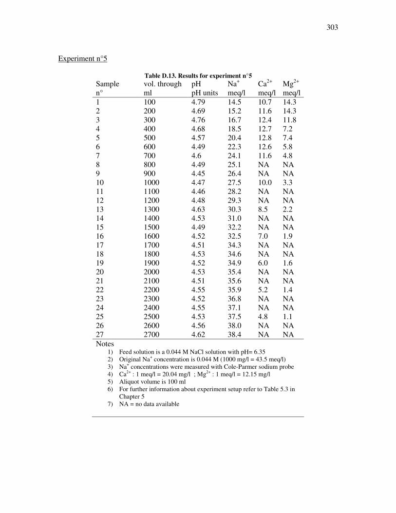
303
Experiment n°5
Table D.13. Results for experiment n°5 Sample vol. through pH Na+ Ca2+ Mg2+ n° ml pH units meq/l meq/l meq/l 1 100 4.79 14.5 10.7 14.3 2 200 4.69 15.2 11.6 14.3 3 300 4.76 16.7 12.4 11.8 4 400 4.68 18.5 12.7 7.2 5 500 4.57 20.4 12.8 7.4 6 600 4.49 22.3 12.6 5.8 7 700 4.6 24.1 11.6 4.8 8 800 4.49 25.1 NA NA 9 900 4.45 26.4 NA NA 10 1000 4.47 27.5 10.0 3.3 11 1100 4.46 28.2 NA NA 12 1200 4.48 29.3 NA NA 13 1300 4.63 30.3 8.5 2.2 14 1400 4.53 31.0 NA NA 15 1500 4.49 32.2 NA NA 16 1600 4.52 32.5 7.0 1.9 17 1700 4.51 34.3 NA NA 18 1800 4.53 34.6 NA NA 19 1900 4.52 34.9 6.0 1.6 20 2000 4.53 35.4 NA NA 21 2100 4.51 35.6 NA NA 22 2200 4.55 35.9 5.2 1.4 23 2300 4.52 36.8 NA NA 24 2400 4.55 37.1 NA NA 25 2500 4.53 37.5 4.8 1.1 26 2600 4.56 38.0 NA NA 27 2700 4.62 38.4 NA NA Notes
1) Feed solution is a 0.044 M NaCl solution with pH= 6.35 2) Original Na+ concentration is 0.044 M (1000 mg/l = 43.5 meq/l) 3) Na+ concentrations were measured with Cole-Parmer sodium probe 4) Ca2+ : 1 meq/l = 20.04 mg/l ; Mg2+ : 1 meq/l = 12.15 mg/l 5) Aliquot volume is 100 ml 6) For further information about experiment setup refer to Table 5.3 in
Chapter 5 7) NA = no data available

304
Sodium absortion using Ngakuru zeolites and a 44 meq/l Na+ solution
05
1015202530354045
0 0.1 0.2 0.3 0.4 0.5 0.6 0.7 0.8 0.9 1 1.1 1.2 1.3 1.4 1.5 1.6 1.7 1.8 1.9 2 2.1 2.2 2.3 2.4 2.5 2.6 2.7
Volume through zeolite column (litres)
meq
/l
[Na] Origina sodium concentration Calcium Magnesium
Figure D.5. Experiment #5: sodium absorption and cation release using Ngakuru zeolites
0.95R
litresin column through volume (meq/l)aliquot samplein ion concentrat sodium [Na]
where,
6.28)ln(8.7 [Na]
2 ==
=
+⋅=
v
v
Eq D.2 Experiment n°6
Table D.14. Fractional isotherm and separation factor for experiment n°6 Solution Solid Separation factor
(c-c')/(c''-c') (q-q')/(q''-q') X Y R 0.00 0.09 0.19 0.17 1.116 0.24 0.25 0.982 0.33 0.32 1.074 0.41 0.38 1.148 0.48 0.50 0.919 0.65 0.60 1.238 0.73 0.69 1.229 0.83 0.77 1.508 0.84 0.84 1.050 0.93 0.90 1.434 0.97 0.95 1.449 1.00 1.00

305
Experiment n°7
Table D.15. Fractional isotherm and separation factor for Experiment n°7 Solution Solid Separation factor
(c-c')/(c''-c') (q-q')/(q''-q') X Y R
0.0 0.0 0.1 0.1 0.978 0.1 0.2 0.884 0.2 0.2 1.139 0.3 0.3 1.135 0.4 0.4 1.117 0.4 0.4 0.888 0.6 0.5 1.528 0.7 0.5 2.103 0.7 0.6 1.976 0.7 0.6 1.308 0.8 0.6 1.807 0.8 0.7 2.523 0.9 0.7 2.242 0.7 0.8 0.738 0.9 0.8 1.534 0.9 0.8 1.758 0.9 0.9 1.122 1.0 0.9 4.696 0.9 0.9 1.227 0.9 1.0 0.278 1.0 1.0
D.4 References
Amphlett, C.B., 1964, Inorganic ion exchangers: Amsterdam, New York,, Elsevier Pub.
Co., x, 141 p. p.
Perry, R.H., Chilton, C.H., and Perry, J.H., 1973, Chemical engineers' handbook: Tokyo,
McGraw-Hill Kogakusha, 1 v. (various pagings) p.

306
E. Appendix E X-ray diffraction results provided by the Geology Department, University of Canterbury

307

308

309

310

311
F. Appendix F
Glossary of Terms Absorption. The “process whereby a chemical is incorporated into the interior of a solid”
(Reddi and Inyang, 2000). A broader definition of absorption is “the process of taking up
and internalizing of a substance by another substance through chemical or molecular
action (e.g. a gas absorbed by a liquid)” (Dooley JJ , 1999).
Accuracy, A measure of the degree of systematic errors being carried out when
conducting a measurement. In this way, small systematic errors produce results of high
accuracy.
Adsorption. The “process of attraction of chemicals to the surface of a solid” (Reddi and
Inyang, 2000). It has also been defined as the accumulation of a chemical at the interface
(Adamson, 1990) of a solid.
Aerobic respiration. A process by which microorganisms consume the electrons
generated by an oxidation reduction reaction in the presence of oxygen. The process is
controlled by the reaction (Snoeyink and Jenkins, 1980):
O2(g) + 4H+ + 4e- � 2H2O

312
Anaerobic respiration. An anoxic process by which microorganisms consume the
electrons generated as reduction reactions take place. Some of the common anaerobic
reactions controlling this process are (Snoeyink and Jenkins, 1980):
Denitrification 2NO3- + 12H+ + 10e- � N2(g) + 6H2O
Nitrate reduction NO3- + 10H+ + 8e- � NH4
+ + 3H2O
Fermentation CH2O + 2H+ + 2e- � CH3OH
Sulphate reduction SO42- + 9H+ + 8e- � HS- + 4H2O
Methane fermentation CO2(g) + 8H+ + 8e- � CH4(g) + 2H2O
Cation Exchange Capacity (CEC). The CEC of a soil (or material) is “defined by the
amount of a cation (such as NH4+, Ba2+) that a soil can hold when a buffered or
unbuffered salt solution is leached through the soil” (Blakemore, 1987).
Cleat. Natural fracture occurring in coal which defines the basic matrix structure of coal.
Cleats form an orthogonal system in coal and are divided into face cleats (dominant cleats
parallel to the maximum compressive stress) and butt cleats (parallel to the fold axis).
Conductivity (electrical conductivity). This is the ability of a solution to conduct an
electrical current. An electrical current is conducted through a solution by the movement
of ions in solution. The higher the dissolved ions concentrations, the higher the
conductivity. It is temperature dependent (see specific conductance) and measured in
mhos/cm or µS/cm (Snoeyink and Jenkins, 1980).

313
Darcy’s Law. An empirical law discovered by Henry Darcy in 1856 which describes
flow through a porous media (Freeze and Cherry, 1979). Darcy’s law can be defined by
the following equation:
lh
Kv∆∆⋅−=
where ∆h = h2 - h1 or the difference in hydraulic head between two given points
∆l = l2 - l1 or the distance between two given points
-K = constant inherent to the porous media and know as hydraulic conductivity (L/T)
v = the speed of liquid flow through the porous media (L/T)
Desorption. The reverse process of Sorption (Reddi and Inyang, 2000).
Diffusion. “The process whereby ionic or molecular constituents move under the
influence of their kinetic activity in the direction of their concentration gradient” (Freeze
and Cherry, 1979).
Exchangeable Sodium Percentage (ESP). This is the ratio (%) of sodium cations to the
total CEC in a given soil. It can be calculated using the following equation:
CECNa
ESP100⋅=
where Na and CEC are the sodium content and cation exchange capacity of the soil both
generally expressed in meq/100g.

314
Fick’s Law (or Fick’s first Law). The law governing the diffusion process: “the mass of
diffusing substance passing through a given cross section per unit time is proportional to
the concentration gradient” (Freeze and Cherry, 1979). This law is generally expressed by:
dxdC
DF ⋅−=
where F = the mass flux (M/L2T)
D = the diffusion coefficient (L2/T)
C = the solute concentration (M/L3)
dC/dx = concentration gradient (negative quantity in the direction of diffusion)
Gas flow test. A pilot operation for CSG well desorption. This involves pumping water
out of a selected well for an extended period of time (months) to obtain relevant data (i.e.
pressure for gas flow, water quality data, and aquifer properties) for CSG extraction.
Hydraulic conductivity (K). As defined in Darcy’s Law definition, K is a measure of the
rate at which a liquid can flow through a porous media. K has “high values for sand and
gravel and low values for clay and most rocks” (Freeze and Cherry, 1979).
Hydraulic gradient. The differential form of ∆h/∆l (= dh /dl) as defined in Darcy’s Law
definition.
Ion exchange. The process of cation substitution in solids, therefore it is often considered
a special case of absorption (Reddi and Inyang, 2000).
Precision. A measure of the extent of random errors being committed. For example, high
precision relates to small random errors.
Random errors. Random fluctuations in measurements that are of a non-deterministic
nature. These fluctuations could originate due to errors of judgment, ambient fluctuations,
mechanical vibrations, and intrinsical random processes to mention a few (Meyer, 1975).

315
Relative error. A measurement of the deviation generated when measuring a property
which has a true value which is known or inferred.
Relative error = δx = ∆x/x
∆x = xo-x
where,
x = true value
xo = measured value
∆x = absolute error�
Relative Standard Deviation (RSD). This is also known as the fractional standard
deviation and is the standard deviation sample population divided by its average. Often
expressed in percentage units.
Salinity. Is the total salt concentration found in water. It can be measured using TDS
(mg/l) or specific conductance (dS/m).
SAR. This is the Sodium Adsortion Ratio and can be calculated for the irrigation water or
for the soil-water solution itself. General guidelines, however, are based on the SAR of
the irrigation water. The SAR value can be calculated using the following equation with
concentrations in meq/l:
2][][
][
MgCa
NaSAR
+=
The SAR value needs to be adjusted for calcium precipitation specially in the presence of
bicarbonate (Ayers, 1985).

316
Sorption. The term commonly used to include all the processes responsible for mass
transfer: absorption, adsorption, and ion exchange (Reddi and Inyang, 2000). The word
“sorbed” can be used to describe how CSG is held in the micropores of coal. That is,
CSG is sorbed when it is contained within the coal micropores, and it is said to be
“desorbed”when it is released by lowering of the piezometric pressure.
Specific conductance (specific conductivity or conductance). Is the conductivity of a
solution measured at a reference temperature of 25°C. This value is usually expressed in
mS/m (Hounslow, 1995).
Systematic errors. Errors of deterministic nature such as calibration errors, biased errors
of judgment, varying efficiencies in observations and experimental conditions (Meyer,
1975).
References Adamson, A.W., 1990, Physical chemistry of surfaces: New York, Wiley, xxi, 777 p.
Ayers, R.S., Westcot, D.W., and Food and Agriculture Organization of the United
Nations., 1985, Water quality for agriculture: Rome, Food and Agriculture
Organization of the United Nations, xii, 174 p.
Blakemore, L.C., Searle, P.L., Daly, B.K., and New Zealand. Soil Bureau., 1987,
Methods for chemical analysis of soils: Lower Hutt, N.Z., NZ Soil Bureau Dept.
of Scientific and Industrial Research, 103 p.
Dooley JJ , and http://energytrends.pnl.gov/index.htm, E.T.s., 1999, Glossary - Energy
R&D, Global Trends in Policy and Investment., Volume 2005.
Freeze, R.A., and Cherry, J.A., 1979, Groundwater: Englewood Cliffs, N.J., Prentice-Hall,
xvi, 604 p.
Hounslow, A., 1995, Water quality data : analysis and interpretation: Boca Raton, Lewis
Publishers, 397 p.
Meyer, S.L., 1975, Data analysis for scientists and engineers: N.Y., Wiley, 513 illus. p.

317
Reddi, L.N., and Inyang, H.I., 2000, Geoenvironmental engineering : principles and
applications: New York, Marcel Dekker, xii, 494 p.
Snoeyink, V.L., and Jenkins, D., 1980, Water chemistry: New York, Wiley, xiii, 463 p.

318
7. Bibliography Adamson, A.W., 1990, Physical chemistry of surfaces: New York, Wiley, xxi, 777 p.
Alabama State Oil and Gas Board (AOGB), 2003, Coalbed Methane Resources of
Alabama http://www.ogb.state.al.us, Volume 2005.
Alabaster, J.S., Lloyd, R., European Inland Fisheries Advisory Commission. Working
Party on Water Quality Criteria for European Freshwater Fish., and European
Inland Fisheries Advisory Commission. Working Party on Toxicity Testing
Procedures., 1980, Water quality criteria for freshwater fish: London,
Butterworths by arrangement with the Food and Agriculture Organization of the
United Nations, xviii, 297 p.
ALL-Consulting, 2003, Handbook on Coal Bed Methane Produced Water: Management
and Beneficial Use Alternatives.: Tulsa, Oklahoma, Ground Water Protection
Research Foundation, US Department of Energy, National Petroleum Technology
Office, Bureau of Land Management.
ALL-Consulting, and Montana Board of Oil and Gas Conservation, 2004, Coal Bed
Methane primer. New Source of Natural Gas–Environmental Implications.
Background and Development in the Rocky Mountain West: Tulsa, Oklahoma,
US Department of Energy, National Petroleum Technology Office.
Allen, R.B., McIntosh, P.D., and Wilson, J.B., 1998, The distribution of plants in relation
to pH and salinity on inland saline/alkaline soils in Central Otago, New Zealand.
(vol 35, pg 517, 1997): New Zealand Journal of Botany, v. 36, p. 153-153.
American Public Health Association., American Water Works Association., and Water
Environment Federation., 1999, Standard methods for the examination of water
and wastewater: Washington, D.C., American Public Health Association, 1
computer optical disc p.
Amphlett, C.B., 1964, Inorganic ion exchangers: Amsterdam, New York,, Elsevier Pub.
Co., x, 141 p. p.
ANZECC, and ARMCANZ, 2000, Australian and New Zealand Guidelines for Fresh and
Marine Water Quality, ACT: Australian and New Zealand Environmental and
Conservation Council (ANZECC), Agricultural and Resource Management

319
Council of Australia and New Zealand (ARMCANZ): Canberra.
Ayers, R.S., Westcot, D.W., and Food and Agriculture Organization of the United
Nations., 1985, Water quality for agriculture: Rome, Food and Agriculture
Organization of the United Nations, xii, 174 p.
Bartos, T.T., Ogle, K.M., Wyoming. State Engineer's Office., United States. Bureau of
Land Management., and Geological Survey (US), 2002, Water quality and
environmental isotopic analyses of ground-water samples collected from the
Wasatch and Fort Union formations in areas of coalbead methane development :
implications to recharge and ground-water flow, eastern Powder River Basin,
Wyoming, Water-resources investigations report ; 02-4045: Cheyenne, Wyo;
Denver, CO, US Dept. of the Interior US Geological Survey, Branch of
Information Services distributor, p. vi, 88 , (4 folded).
Bauder, J., 2001, Quality and Characteristics of Saline and Sodic Water Affect Irrigation
Suitability: MSU, Bozeman, MT, p. http://waterquality.montana.edu.
Blakemore, L.C., Searle, P.L., Daly, B.K., and New Zealand. Soil Bureau., 1987,
Methods for chemical analysis of soils: Lower Hutt, N.Z., NZ Soil Bureau Dept.
of Scientific and Industrial Research, 103 p.
Bodger, F., 2005, The use of coal seam gas waters in New Zealand to treat acid mine
drainage, Civil Engineering: Christchurch, University of Canterbury, p. 44.
Boelter, A.M., Lamming, F.N., Farag, A.M., and Bergman, H.L., 1992, Environmental
effects of saline oil-field discharges on surface waters: Environmental Toxicology
and Chemistry, v. 11, p. 1187-1195.
Bolan, N.S., and Mowat, C., 2000, Potential value of zeolite in the removal of
contaminants from wastewater stream, Water 2000, Water Conference and Expo,
"Guarding the Global Resource": Auckland, NZWWA, p. 430-443.
Bresler, E., McLean, B.L., and Carter, D.L., 1982, Saline and sodic soils: Principles-
dynamics-modeling., Advanced series in agricultural sciences., Volume 10: New
York, NY, Springer-Verlag.
Bryant, F.B., and Yarnold, P.R., 1995, Principal components analysis: Thousand Oaks,
CA, Sage Publications.
Burkett, W.C., McDaniel, R., and Hall, W.L., 1991, The Evaluation and Implementation

320
of a Comprehensive Production Water Management Plan, Coalbed Methane
Symposium: Tuscaloosa, Alabama.
Cameron, K.C., Di, H.J., Anwar, M.R., Russell, J.M., and Barnett, J.W., 2003, The
"critical" ESP value: does it change with land application of dairy factory
effluent?: New Zealand Journal of Agricultural Research, v. 46, p. 147-154.
Carothers, W.W., and Kharaka, Y.K., 1980, Stable carbon isotopes of HCO3- in oil-field
waters--implications for the origin of CO2: Geochimica et Cosmochimica Acta, v.
44, p. 323-332.
Cavanagh, J., and Coakley, J., 2005, An introduction to policy on metal contaminants, in
Moore, T.A., Black, A., Centeno, J.A., Harding, J.S., and Trumm, D.A., eds.,
Metal Contaminants in New Zealand, Volume In Press, Corrected Proof:
Christchurch, resolutionz press, p. 5-23.
Cave, M., 2002, Turning a coalbed methane project into a co-producing hydrocarbon
project, 2002 New Zealand Petroleum Conference proceedings: Wellington, N.Z.,
New Zealand Crown Minerals, p. 13.
Cave, M., and Syme, A., 2002, Impact of Operational and Environmental Issues on the
development of Coalseam Gas in New Zealand, 2004 New Zealand Petroleum
Conference proceedings: Wellington, N.Z., New Zealand Crown Minerals, p. 11.
Chapelle, F., 2001, Ground-water microbiology and geochemistry: New York, N.Y.,
Wiley, xvii, 477 p.
Chatfield, C., 1996, The analysis of time series : an introduction: London, Chapman &
Hall, xii, 283 p.
Christie, T., Brathwaite, B., and Thomson, B., 2002, Mineral Commodity Report 23 -
Zeolites, New Zealand Mining, Volume 31.
Clark, I.D., and Fritz, P., 1997, Environmental isotopes in hydrogeology: Boca Raton, FL,
CRC Press/Lewis Publishers, 328 p. p.
Claypool, G.E., and Kaplan, I.R., 1974, The origin and distribution of methane in marine
sediments: Marine Science, v. 3, p. 99-139.
Collier, K.J., Ball, O.J., Graesser, A.K., Main, M.R., and Winterbourn, M.J., 1990, Do
organic and anthropogenic acidity have similar effects on aquatic fauna?: Oikos, v.
59, p. 33-38.

321
Colorado Oil and Gas Conservation Comission, 2001, Webpage database for production.
Comrey, A.L., and Lee, H.B., 1992, A first course in factor analysis: Hillsdale, N.J., L.
Erlbaum Associates, xii, 430 p.
Coombs, D.S., 1959, Zeolite uses and New Zealand deposits, Fourth Triennial Mineral
Conference, Volume 6, Paper 162: School of Mines and Metallurgy, Dunedin,
University of Otago, p. 6.
Curtin, D., Steppuhn, H., and Selles, F., 1994, Structural Stability of Chernozemic Soils
as Affected by Exchangeable Sodium and Electrolyte Concentration: Canadian
Journal of Soil Science, v. 74, p. 157-164.
Davies-McConchie, F., McConchie, D., Clark, M., Lin, C., Pope, S., and Ryffel, T., 2002,
A new approach to the treatment and management of sulphidic mine tailings,
waste rock and acid mine drainage: New Zealand Mining, v. 31, p. 7-15.
Davis, H.A., Simpson, T.E., Lawrence, A.W., Miller, J.A., and Anonymous, 1993,
Coalbed methane produced water management strategies in the Black Warrior
Basin of Alabama: Proceedings - International Coalbed Methane Symposium, v.
1993, p. 317-338.
Davis, J.C., 2002, Statistics and data analysis in geology: New York, J. Wiley, xvi, 638 p.
p.
Davis, W.N., Bramblett, R.G., and Zale, A.V., 2006, The effects of coalbed natural gas
activities on fish assemblages: a review of the literature: Bozeman, Montana State
University, p. 48.
—, 2006, Effects of coalbed natural gas activities on fish assemblages in the Powder
River Basin, 2005, in Montana Cooperative Fishery Research Unit, ed.: Bozeman,
Montana State University, p. 3.
Decker, A.D., Klusman, R., Horner, D.M., and Anonymous, 1987, Geochemical
techniques applied to the identification and disposal of connate coal water:
Proceedings - International Coalbed Methane Symposium, v. 1987, p. 229-242.
Deffeyes, K.S., 1965, The Deffeyes diagram for 25°C: Limnology and Oceanography, v.
10, p. 412.
Deidre B. Boysen, J.E.B., Jessica A. Boysen, 2002, Strategic produced water
management and disposal economics in the Rocky Mountain Region, Ground
322
water protection council.
Department of Conservation, 2006, New Zealand map service, DOCgis GeoSpatial
Information Platform, p. http://extranet.doc.govt.nz/bip/.
—, 2006, New Zealand's Wetlands of International Significance: Whangamarino,
http://www.doc.govt.nz/Conservation/Wetlands/.
Detmer, E., 2005, Zeolite water conditioning system: Sheridan, p. Personal conversation.
Dooley JJ , and http://energytrends.pnl.gov/index.htm, E.T.s., 1999, Glossary - Energy
R&D, Global Trends in Policy and Investment., Volume 2005.
Edbrooke, S.W., Sykes, R., and Pocknall, D.T., 1994, Geology of the Waikato Coal
Measures, Waikato Coal Region, New Zealand., Institute of Geological &
Nuclear Sciences Monograph, p. 236.
Eisler, R., 1991, Cyanide Hazards to Fish, Wildlife, and Ivertebrates, US Fish and
Wildlife Service.
Energy Information Administration, 2004, Advance Summary: US Crude Oil, Natural
Gas, and Natural Gas Liquids Reserves 2003 Annual Report: Washington, DC
20585, Office of Oil and Gas, US Department of Energy, p. 18.
Environment Waikato, 2002, Waikato Regional Plan - Proposed plan and maps on CD-
ROM as amended by decisions (appeals version), in Waikato Regional Council,
ed.: Hamilton, Waikato Regional Council,.
Environment Waikato, 2006, River Levels and Rainfall. Whangamarino Wetland. Levels
at Ropeway on Island Block Road, Meremere, Volume 2006: Hamilton,
Environment Waikato, p. web page and online database system.
Eser, P., and Rosen, M.R., 2000, Effects of artificially controlling levels of Lake Taupo,
North Island, New Zealand, on the Stump Bay wetland: New Zealand Journal of
Marine and Freshwater Research, v. 34, p. 217-230.
Freeze, R.A., and Cherry, J.A., 1979, Groundwater: Englewood Cliffs, N.J., Prentice-Hall,
xvi, 604 p.
Gamson, P.D., Beamish, B.B., and Johnson, D.P., 1993, Coal Microstructure and
Micropermeability and Their Effects on Natural-Gas Recovery: Fuel, v. 72, p. 87-
99.
—, 1996, Coal Microstructure and Micropermeability and Their Effects on Natural-Gas

323
Recovery, in Gayer, R.A., and Harris, I.H., eds., Coalbed methane and coal
geology: London, Geological Society, p. 165-179.
Gas Technology Institute, 2002, http://www.gastechnology.org/.
Gayer, R.A., and Harris, I.H., 1996, Coalbed methane and coal geology: London,
Geological Society, viii, 344 p.
Gilbert, R.O., 1987, Statistical methods for environmental pollution monitoring: New
York, Van Nostrand Reinhold Co., x, 320 p.
Gillard, G., Trumm, D., Manhire, D., Taulis, M., and Muckle, F., 2003, Final Report
Exploration Permit 40 396 Hawkdun: Christchurch, CRL Energy Ltd, p. 51.
GRI (Gas Research Institute), 2000, Coalbed Methane Potential of the US Rocky
Mountain Region, p. 3pp.
Haan, C.T., 1977, Statistical methods in hydrology: Ames, Iowa State University Press,
xv, 378 p.
Hach Company, 2003, Water analysis handbook : drinking water, wastewater, seawater,
boiler/cooling water, ultrapure water: Loveland, Colo., Hach, 1268 p.
Hagmaier, J.L., 1971, Groundwater flow, hydrogeochemistry, and uranium deposition in
the Powder River Basin, Wyoming [Ph.D thesis]: Grand Forks, University of
North Dakota, Department of Geology.
Hamilton, T.M., 1970, Groundwater flow in part of the Little Missouri River Basin,
North Dakota [Ph.D thesis]: Grand Forks, University of North Dakota,
Department of Geology.
Hatcher, L., 1994, A step-by-step approach to using the SAS system for factor analysis
and structural equation modeling: Cary, N.C., SAS Institute, xiv, 588 p.
Hem, J.D., 1985, Study and interpretation of the chemical characteristics of natural water,
U. S. Geological Survey Water-Supply Paper, p. 263.
Higgins, C.L., and Wilde, G.R., 2005, The role of salinity in structuring fish assemblages
in a prairie stream system: Hydrobiologia, v. 549, p. 197-203.
Hoffman, R.D., and Animated Software Company., 2004, Internet glossary of pumps:
[California], Animated Software Co.
Hounslow, A., 1995, Water quality data : analysis and interpretation: Boca Raton, Lewis
Publishers, 397 p.

324
IEA Coal Industry Advisory Board., 1994, Global methane and the coal industry : a two-
part report on methane emissions from the coal industry and coalbed methane
recovery and use: Paris.Washington, D.C., OECD; OECD Publications and
Information Centre distributor, 67 p.
Jenden, P.D., and Kaplan, I.R., 1986, Comparison of microbial gases from the Middle
America Trench and Scripps Submarine Canyon: implications for the origin of
natural gas: Applied Geochemistry, v. 1, p. 631-646.
Jensen, M.E., 1983, Design and operation of farm irrigation systems: St. Joseph, Mich.,
American Society of Agricultural Engineers, xi, 829 p. p.
Ji, Z.-G., 2005, Water quality models: chemical principles: Hoboken, New Jersey., John
Wiley and Sons, Inc.
Johnson, K.C., 2004, The New Zealand coal seam gas scene, 2004 New Zealand
Petroleum Conference proceedings: Wellington, N.Z., New Zealand Crown
Minerals, p. 7.
Kaiser, H.F., 1958, The Varimax Criterion for Analytic Rotation in Factor-Analysis:
Psychometrika, v. 23, p. 187-200.
Karassik, I.J., 1986, Pump handbook: New York, McGraw-Hill, 1 v. (various pagings) p.
Kirkpatrick, A., Pearson, K., and Bauder, J., 2003, The Use of Coal Bed Methane Product
Water to Enhance Wetland Function: MSU, Bozeman, MT, p. 11.
Kirkpatrick, A.D., 2005, Assessing constructed wetlands for beneficial use of saline-sodic
water: Bozeman, Montana State University,.
Kjeldsen, P., Barlaz, M.A., Rooker, A.P., Baun, A., Ledin, A., and Christensen, T.H.,
2002, Present and Long-Term Composition of MSW Landfill Leachate: A Review:
Critical Reviews in Environmental Science and Technology, v. 32, p. 297-336.
Knight, R.L., 1997, Wildlife habitat and public use benefits of treatment wetlands: Water
Science and Technology, v. 35, p. 35-43.
Krevelen, D.W.v., 1961, Coal: typology, chemistry, physics, constitution: Amsterdam,
New York,, Elsevier Pub. Co., xviii, 514 p.
Kristin, K., Bauder, J., and Wheaton, J.R., 2006,
http://waterquality.montana.edu/docs/methane/cbmfaq.shtml, Water quality and
Irrigation Management, Volume 2006: Bozeman, Montana State University.
325
Kuuskraa, V.A., 1989, Coalbed Methane Sparks a New Energy Industry: Oil & Gas
Journal, v. 87, p. 49-&.
Landcare Research New Zealand Ltd, 2000, The New Zealand National Soils Database
Spatial Extension, Soil Fundamental Data Layers: Lincoln, Landcare Research
New Zealand Ltd.
—, 2000, New Zealand Land Resource Inventory (NZLRI): Lincoln, Landcare Research
New Zealand Ltd.
Law, B.E., and Rice, D.D., 1993, Hydrocarbons from coal: Tulsa, Okla., USA, American
Association of Petroleum Geologists, viii, 400 p.
Lee, R.W., 1981, Geochemistry of water in the Fort Union Formation of the northern
Powder River Basin, southeastern Montana, U. S. Geological Survey Water-
Supply Paper.
Lee-Ryan, P.B., Fillo, J.P., Tallon, J.T., and Evans, J.M., 1991, Evaluation of
management options for coalbed methane produced water, Coalbed methane
symposium: Tuscaloosa, Alabama, The University of Alabama,, p. 31-41.
LFTB Study Group., 1986, South Island Phase II Lignite Site Selection Studies
Programme. Resource definition, geotechnical, hydrology, and mine planning
studies. Hawkdun deposit.: Wellington, N.Z., Liquid Fuels Trust Board.
Main, M.R., 1988, Factors influencing the distribution of kokopu and koaro (Pisces:
Galaxiidae) : a thesis submitted in partial fulfilment of the requirements for the
degree of Master of Science in Zoology in the University of Canterbury, 127
leaves, [36] leaves of plates p.
Maloszewski, P., and Zuber, A., 1982, Determining the Turnover Time of Groundwater
Systems with the Aid of Environmental Tracers .1. Models and Their
Applicability: Journal of Hydrology, v. 57, p. 207-231.
Matalas, N.C., and Reiher, B.J., 1967, Some Comments on Use of Factor Analyses:
Water Resources Research, v. 3, p. 213-&.
McBeth, I., Reddy, K.J., and Skinner, Q.D., 2003, Chemistry of trace elements in coalbed
methane product water: Water Research, v. 37, p. 884-890.
McBeth, I.H., Reddy, K.J., and Skinner, Q.D., 2003, Coalbed methane product water
chemistry in three Wyoming watersheds: Journal of the American Water

326
Resources Association, v. 39, p. 575-585.
McIntosh, A., and McDowall, R., 2004, Fish Communities in rivers and streams, in
Harding, J.S., New Zealand Hydrological Society., and New Zealand
Limnological Society., eds., Freshwaters of New Zealand: [Wellington, N.Z.],
New Zealand Hydrological Society ; New Zealand Limnological Society, p. 17.1-
17.9.
McLaren, R.G., and Cameron, K.C., 1990, Soil science : an introduction to the properties
and management of New Zealand soils: Auckland, N.Z., Oxford University Press,
viii, 294 , 8 of plates p.
Menneer, J.C., McLay, C.D.A., and Lee, R., 2001, Effects of sodium-contaminated
wastewater on soil permeability of two New Zealand soils: Australian Journal of
Soil Research, v. 39, p. 877-891.
Meyer, S.L., 1975, Data analysis for scientists and engineers: N.Y., Wiley, 513 illus. p.
Milke, M.W., and Huitric, R.L., 1993, Simulating Errors in Statistical Tests of Leachate-
Impacted Groundwater Quality: Ground Water, v. 31, p. 645-653.
MINITAB Inc, 2005, MINITAB, Volume 2005: Pennsylvania.
Montana Board of Oil and Gas Conservation, 2005, On-Line Data,
http://bogc.dnrc.state.mt.us.
Montana State University, 2006, Frequently Asked Questions Coal Bed Methane (CBM),
Volume 2006: Bozeman, Montana State University, p. Web page
http://waterquality.montana.edu/docs/methane/cbmfaq.shtml.
—, 2006, Coal Bed Methane Water Treatment System,
http://waterquality.montana.edu/docs/methane/cbm-wts.shtml, Montana State
University., p. Drake Engineering Inc. Water Treatment System.
Montgomery, S.L., 1999, Powder River Basin, Wyoming: An expanding coalbed
methane (CBM) play: Aapg Bulletin-American Association of Petroleum
Geologists, v. 83, p. 1207-1222.
Montgomery, S.L., Tabet, D.E., and Barker, C.E., 2001, Upper Cretaceous Ferron
Sandstone: Major Coalbed Methane Play in Central Utah: AAPG Bulletin, v. 85,
p. 199-219.

327
Moore, T.A., Manhire D.A., Flores R.M., 2002, Coalbed Methane opportunities in New
Zealand: Similarities with the Powder River Basin coalbed methane paradigm,
AusIMM Conference: Auckland, New Zealand.
Moore, T.A., and Shearer, J.C., 2003, Peat/coal type and depositional environment - Are
they related?: International Journal of Coal Geology, v. 56, p. 233-252.
Mount, D.R., Drottar, K.R., Gulley, D.D., and Fillo, J.P., 1993, Use of Laboratory
Toxicity Data for Evaluating the Environmental Acceptability of Produced Water
Discharge to Surface Waters, v. 46, p. 175.
Mount, D.R., O'Neil, P.E., and Evans, J.M., 1993, Discharge of coalbed product water to
surface waters: assessing, predicting, and preventing ecological effects: Quarterly
Review of Methane from Coal Seams Technology, v. 11, p. 18-25.
Mowatt, C., 2000, Preliminary investigations into the characteristics and potential uses
for Ngakuru zeolites, 2000 New Zealand Minerals & Mining Conference
Proceedings.
Nelson, C.R., 2005, Geologic assessment of the natural gas resources in the Powder River
Basin Fort Union Formation coal seams, Proceedings - International Coalbed
Methane Symposium, Volume 2005, p. 14.
New Mexico Oil Conservasion Division, New Mexico Energy, Minerals and Natural
Resources Department - OCD Webpage, Development RBDMS.
New Zealand. Mines Division., Longworth McKenzie Cole., and Worley Consultants
Ltd., 1983, New Zealand coal resources survey : preliminary mining and
environmental constraints assessment pilot study : Maramarua coalfield:
[Wellington, N.Z.], Mines Division Ministry of Energy, 2 v. p.
New Zealand. Ministry of Health., and New Zealand. National Drinking-Water Standards
Review Expert Working Group., 2000, Drinking-water standards for New
Zealand, 2000: Wellington, N.Z., Ministry of Health, xiii, 130 p.
Nguyen, M.L., and Tanner, C.C., 1998, Ammonium removal from wastewaters using
natural New Zealand zeolites: New Zealand Journal of Agricultural Research, v.
41, p. 427-446.
Nielsen, D., 1990, Practical handbook of ground-water monitoring: Chelsea, MI, Lewis
Publishers, x, 717 p.

328
NIWA, 2006, NIWA Atlas of New Zealand Freshwater Fishes, Common smelt
(Retropinna retropinna),
http://www.niwascience.co.nz/rc/freshwater/fishatlas/species/common_smelt,
Volume 2006, NIWA.
—, 2006, NZFFD, New Zealand Freshwater Fish Database, NIWA, p.
http://fwdb.niwa.co.nz/.
Nobes, D.C., and Schneider, G.W., 1996, Results of downhole geophysical measurements
and vertical seismic profile from the Canandaigua borehole of New York State
Finger Lakes: Special Paper - Geological Society of America, v. 311, p. 51-63.
Nuccio, V.F., 2002, Coalbed Methane- What is it? Where is it? And why all the fuss?,
Coalbed methane of North America, II Rocky Mountain Association of
Geologists, 2002: Denver, Colo., The Rocky Mountain Association of Geologists,
p. 6.
NZ Natural Zeolite, 2006, What is Zeolite?, www.zeolite.co.nz.
O'Neil, P.E., Harris, S.C., and Mettee, M.F., 1989, Stream Monitoring of Coalbed
Methane Produced Water from the Cedar Cove Degasification Field, Alabama,
The 1989 Coalbed Methane Symposium: Tuscaloosa, Alabama, The University of
Alabama,.
O'Neil, P.E., Harris, S.C., Mettee, M.F., McGregor, S.W., and Shepard, T.E., 1991,
Long-term biomonitoring of a product water discharge from the Cedar Cove
degasification field, Alabama, Geological Survey of Alabama (Bulletin),
Tuscaloosa, Volume 141.
Oremland, R.S., Marsh, L.M., and Polcin, S., 1982, Methane Production and
Simultaneous Sulfate Reduction in Anoxic, Salt-Marsh Sediments: Nature, v. 296,
p. 143-145.
Oster, J.D., and Schroer, F.W., 1979, Infiltration as Influenced by Irrigation Water-
Quality: Soil Science Society of America Journal, v. 43, p. 444-447.
Perry, R.H., Chilton, C.H., and Perry, J.H., 1973, Chemical engineers' handbook: Tokyo,
McGraw-Hill Kogakusha, 1 v. (various pagings) p.
Pope, S., 2004, Coal Seam Gas Exploration Results: Hawkdun Coalfield, Central Otago,
2002-2004.: Christchurch, CRL Energy Ltd, p. 42.

329
—, 2004, 2004 Coal Seam Gas Exploration Results: Ashers-Waituna Lignite Deposit,
PEP 38-217, Southland.: Christchurch, CRL Energy Ltd, p. 41.
Pope, S., and Trumm, D., 2004, Coal Seam Gas Desorption Results: Drill Holes C1, K1
and K3, Maramarua Coalfield, Waikato, 2003.: Christchurch, CRL Energy Ltd, p.
27.
PTTC, 2000, Coal bed methane strategraphic traps in the ferron coals of east-central Utah,
PTTC Rocky Mountain Newsletter, Volume September.
Ralph J. Haefner, and US Geological Survey, 2002, Water Quality at an Abandoned Coal
Mine Reclaimed with PFBC By-Products: Columbus, Ohio, US Geological
Survey, p. 37.
Reddi, L.N., and Inyang, H.I., 2000, Geoenvironmental engineering : principles and
applications: New York, Marcel Dekker, xii, 494 p.
Rhoades, J.D., 1982, Reclamation and management of salt-affected soils after drainage.
In Rationalisation of water
and soil research and management, Proceedings of the First Annual Western Provincial
Conference: Lethbridge, Canada, p. 123–197.
Rice, C.A., and Anonymous, 1999, Waters co-produced with coalbed methane from the
Ferron Sandstone in east-central Utah; chemical and isotopic composition,
volumes, and impacts of disposal: Abstracts with Programs - Geological Society
of America, v. 31, p. 385.
Rice, C.A., and Bartos, T.T., 2001, Nature and Characteristics of Water Co-Produced
with Coalbed Methane with emphasis on the Powder River Basin, USGS Coalbed
Methane Field conference May 9-10, 2001., Volume Open File Report 01-235:
Casper, Wyoming., USGS.
Rice, C.A., Breit, G.N., Hills, F.A., and Anonymous, 1993, Variations of Mg, Sr, and K
in sulfate minerals from the Paradox Formation, Utah; clues to the composition of
depositional and diagenetic brines: Abstracts with Programs - Geological Society
of America, v. 25, p. 253.
Rice, C.A., Ellis, M.S., and Bullock, J.H., Jr., 2000, Water co-produced with coalbed
methane in the Powder River Basin, Wyoming: preliminary compositional data:
Open-File Report - U. S. Geological Survey.

330
Rice, D.D., 1992, Controls, habitat, and resource potential of ancient bacterial gas, in
Vially, R., ed., Bacterial gas : proceedings of the conference held in Milan,
September 25-26, 1989: Paris, Editions Technip, p. 91-118.
—, 1993, Composition and origin of coalbed gas, in Law, B.E., and Rice, D.D., eds.,
Hydrocarbons from coal, Volume AAPG Studies in Geology, American
Association of Petroleum Geologists, p. 159-184.
Rice, D.D., and Claypool, G.E., 1981, Generation, accumulation, and resource potential
of biogenic gas: AAPG Bulletin, v. 65, p. 5-25.
Robb, M.R., 2000, Information on water allocation in New Zealand, Lincoln
Environmental Client Report 4375/1, Ministry for the Environment, p. 180.
Robinson, K.M., 2003, Effects of saline-sodic water on EC, SAR, and water retention:
Bozeman, Montana State University.
Rosen, M.R., 2001, Hydrochemistry of New Zealand's Aquifers, in Rosen, M.R., and
White, P.A., eds., Groundwaters of New Zealand: Wellington, New Zealand, New
Zealand Hydrological Society, p. 77-110.
Rosen, M.R., and White, P.A., 2001, Groundwaters of New Zealand: Wellington, N.Z.,
New Zealand Hydrological Society, xiii, 498 p.
Russell, L.L., 1976, Chemical aspects of groundwater recharge with wastewaters:
Berkeley, University of California.
Salmon, J.E., and Hale, D.K., 1959, Ion exchange; a laboratory manual: London,,
Butterworths Scientific Publications, 136 p. p.
Sanders, F., Gustin, S., and Pucel, P., 2001, Natural treatment of CBM produced water:
field observations., CBM Associates Inc.,, Funded by Marathon Oil Company.
Scarsbrook, M.R., and National Institute of Water and Atmospheric Research (N.Z.),
2003, A guide to the groundwater invertebrates of New Zealand: Wellington
[N.Z.], Niwa, 59 p.
Schoell, M., 1980, The hydrogen and carbon isotopic composition of methane from
natural gases of various origins: Geochimica et Cosmochimica Acta, v. 44, p.
649-661.
Schwochow, S.D., Nuccio, V.F., Rocky Mountain Association of Geologists., Gas
Research Institute., and Petroleum Technology Transfer Council (US), 2002,

331
Coalbed methane of North America, II Rocky Mountain Association of
Geologists, 2002: Denver, Colo., The Association, vi, 108 p.
Settle, T., Mollock, G.N., Hinchman, R.R., and Negri, M.C., 1998, Engineering the use of
green plants to reduce produced water disposal volume., Society of Petroleum
Engineers: Inc. Devon Energy Corporation, Oklahoma City, OK. Argonne
National Laboratory, Argonne IL.
Shainberg, I., and Letey, J., 1984, Response of Soils to Sodic and Saline Conditions:
Hilgardia, v. 52, p. 1-57.
Shapiro, S.S., and Wilk, M.B., 1965, An Analysis of Variance Test for Normality
(Complete Samples): Biometrika, v. 52, p. 591-&.
Shaw, R.J., 1996, A unified soil property and sodicity model of salt leaching and water
movement [PhD thesis], University of Queensland.
Shaw, R.J., Thorburn, P.J., and Dowling, A.J., 1987, Principles of landscape, soil and
water salinity: Processes and management options, Proceedings of Brisbane
Region Salinity
Workshop: Part A, in Landscape, soil and water salinity: Brisbane, Queensland
Department of Primary Industries.
Skaar, D., Farag, A., and Harper, D., 2005, National pollution discharge elimination
system. Toxicity of the major salt (sodium bicarbonate) from coalbed methane
production to fish in the Tongue and Powder river drainages in Montana, Semi-
annual progress report prepared for US Environmental Protection Agency: Helena.
Skaar, D., Morris, B., and Farag, A., 2004, National pollution discharge elimination
system. Toxicity of the major salt (sodium bicarbonate) from coalbed methane
production to fish in the Tongue and Powder river drainages in Montana, Progress
report prepared for US Environmental Protection Agency: Helena.
Slater, M.J., 1991, Principles of ion exchange technology: Oxford [England] ; Boston,
Butterworth Heinemann, xiii, 182 p.
Snoeyink, V.L., and Jenkins, D., 1980, Water chemistry: New York, Wiley, xiii, 463 p.
Soil Improvement Committee, 1995, Western fertilizer handbook: Danville, Ill., Interstate
Publishers, xiii, 338 p., [12] p. of plates p.
Stach, E., 1982, Stach's textbook of coal petrology: Berlin, Borntraeger, 535 p.

332
Stumm, W., and Morgan, J.J., 1996, Aquatic chemistry : chemical equilibria and rates in
natural waters: New York, Wiley, xvi, 1022 p.
Suarez, D.L., 1981, Relationship between pHc and sodium adsorption ratio (SAR) and an
alternative method of
estimating SAR of soil or drainage waters: Soil Science Society of America Journal, v. 45,
p. 469-475.
Sumner, M.E., 1992, The electrical double layer and clay dispersion, in Sumner, M.E.,
and Stewart, B.A., eds., Soil crusting: chemical and physical processes, Volume
Adv. Soil Sci.: Boca Raton, FL, Lewis Publishers.
Tabachnick, B.G., and Fidell, L.S., 2001, Using multivariate statistics: Boston, Allyn and
Bacon, xxvi, 966 p.
Taulis, M., Milke, M., Trumm, D., O'Sullivan, A., Nobes, D., and Manhire, D., 2005,
Characterisation of Coal Seam Gas waters in New Zealand, 2005 New Zealand
Minerals Conference: Auckland, New Zealand.
The Seacreast Group, 2003, Water quality data collected from water wells in the Raton
basin, Colorado: Denver, Colorado, Colorado Oil and Gas State Conservation
Comission.
Todd, D.K., 1980, Groundwater hydrology: New York, Wiley, xiii,535 p.
Trumm, D., Black, A., Gordon, K., Cavanagh, J., O’Halloran, K., and de Joux, A., 2005,
Acid mine drainage assessment and remediation at an abandoned West Coast coal
mine, Metal Contaminants in New Zealand: Christchurch, resolutionz.
US Environmental Protection Agency, 2004, Evaluation of Impacts to Underground
Sources of Drinking Water by Hydraulic Fracturing of Coalbed Methane
Reservoirs, US Environmental Protection Agency.
US Environmental Protection Agency, 2004, Statistical Primer, Volume 2005, p. web
page.
US Environmental Protection Agency, 2004, 2005, Exposure Assessment Models, US
Environmental Protection Agency, p. web page.
US Environmental Protection Agency, and Advanced Resources International, 2002,
Enhanced CBM Recovery, US Environmental Protection Agency.
US Geological Survey, 2000, Coal bed methane: potential and concerns, USGS Fact

333
Sheet FS-123-00.
—, 2000, Water Produced with Coal-Bed Methane, USGS Fact Sheet FS-156-00.
US Salinity Laboratory Staff, 1954, Diagnosis and improvement of saline and alkali soils:
[Washington,, US Govt. Print. Off.], vii, 160 p. p.
UCLA Academic Technology Services, Factor Analysis Using SAS PROC FACTOR, in
Services, U.A.T., ed., Volume 2005: Los Angeles, p. Web page.
Van Voast, W.A., 2003, Geochemical signature of formation waters associated with
coalbed methane: Aapg Bulletin, v. 87, p. 667-676.
Van Voast, W.A., and Anonymous, 1991, Hydrogeologic aspects of coal-bed methane
occurrence, Powder River Basin: AAPG Bulletin, v. 75, p. 1142-1143.
Van Voast, W.A., and Hedges, R.B., 1975, Hydrogeologic aspects of existing and
proposed strip coal mines near Decker, Southeastern Montana.: Bulletin -
Montana Bureau of Mines and Geology, v. 97, p. 31.
Vially, R., Azienda generale italiana petroli., International Union of Geological Sciences.,
and Institut franðcais du pâetrole., 1992, Bacterial gas : proceedings of the
conference held in Milan, September 25-26, 1989: Paris, Editions Technip, x, 242
p.
Wachinski, A.M., and Etzel, J.E., 1997, Environmental ion exchange : principles and
design: Boca Raton, CRC/Lewis Publishers, 136 p. p.
Wallis, J.R., 1967, When Is It Safe to Extend a Prediction Equation - an Answer Based
Upon Factor and Discriminant Function Analysis: Water Resources Research, v. 3,
p. 375-&.
Wesolowski, D.J., 1992, Aluminum speciation and equilibria in aqueous solution: I. The
solubility of gibbsite in the system Na-K-Cl-OH-Al(OH)4 from 0 to 100[deg]C:
Geochimica et Cosmochimica Acta, v. 56, p. 1065-1091.
West, D.W., Boubée, J.A.T., and Barrier, R.F.G., 1997, Responses to pH of nine fishes
and one shrimp native to New Zealand freshwaters: New Zealand Journal of
Marine and Freshwater Research, v. 31, p. 461-468.
Wheaton, J.R., Bobst, A.L., Donato, T.A., and Anonymous, 2004, Ground-water
monitoring in the Powder River Basin, southeastern Montana: Abstracts with
Programs - Geological Society of America, v. 36, p. 187.

334
Wheaton, J.R., and Donato, T.A., 2004, COALBED-METHANE BASICS: Powder River
Basin, Montana: Butte, Montana Bureau of Mines and Geology, p. 20.
Whiticar, M.J., Faber, E., and Schoell, M., 1986, Biogenic methane formation in marine
and freshwater environments: CO2 reduction vs. acetate fermentation--Isotope
evidence: Geochimica et Cosmochimica Acta, v. 50, p. 693-709.
Williams, W.D., 2001, Anthropogenic salinization of inland waters: Hydrobiologia, v.
466, p. 329-337.
Williams. B, 2001, Personal communication between Mr. Williams/ V.P., Redstone and
Dr. Langhus/ALL-LLC. March 23, 2001.
Woltemate, I., Whiticar, M.J., and Schoell, M., 1984, Carbon and hydrogen isotopic
composition of bacterial methane in a shallow freshwater lake: Limnology and
Oceanography, v. 29, p. 985-992.
Wyoming State Engineers Office, and Wyoming State Geological Survey, 2005, The
Coal Section.