harvesting energy from decelerating vehicles - web.wpi.edu · 2.5 speed bumps 9 chapter 3. design...
TRANSCRIPT

1
Harvesting Energy from Decelerating Vehicles
A Major Qualifying Project
Submitted to the Faculty of
WORCESTER POLYTECHNIC INSTITUTE
In partial fulfillment of the requirements for the
Degree of Bachelor Science
In Mechanical Engineer and Electrical and Computer Engineering
By:
Kurt J Bilis
Mary Ellen B Osler
Samuel N Smith
Date: 3/23/2018
Approved by:
___________________________________________________
John Sullivan
___________________________________________________
Alexander Emanuel

i
Abstract
In this project we designed and created a prototype capable of harvesting kinetic energy
normally converted to heat by vehicles during braking and converted it to electrical energy to be
used to power nearby streetlights. A slider crank mechanism converted linear motion to radial
motion and a permanent magnet generator that we designed and prototyped created a system to
accomplish this energy harvest. The system was designed to have minimal impact on vehicle
operators and/or passengers.

ii
Acknowledgements
We would like to thank our advisor, Professor Sullivan for his guidance and advice
throughout our design process. We would also like to thank our co-advisor, Professor Emanuel
for his advice on the electrical component of this project. We express gratitude towards the
Mechanical Engineering and Electrical and Computer Engineering departments of WPI for
allowing us to use their facilities and for ordering parts for the prototype.

iii
List of Tables
Table 1: Inertia study for full-scale ramp ..................................................................................... 40
Table 2: Inertia study for the prototype model ramp .................................................................... 43

iv
List of Figures
Figure 1: Completed prototype ....................................................................................................... 1
Figure 2: Piezoelectric device ......................................................................................................... 4
Figure 3: Map of daily traffic through Worcester County [5] ........................................................ 5
Figure 4: Comparison of power efficiency between HPS and LED street lights [2] ...................... 7
Figure 5: Current generated by an armature from two angles [20] ................................................. 8
Figure 6: Diagram of a PMG [12]................................................................................................... 9
Figure 7: Speed bump vs. speed hump [6] .................................................................................... 10
Figure 8: Springboard design ........................................................................................................ 11
Figure 9: Rack and pinion ............................................................................................................. 12
Figure 10: Before the ramp ........................................................................................................... 13
Figure 11: Beginning of ramp ....................................................................................................... 13
Figure 12: Just before the end of the ramp ................................................................................... 13
Figure 13: Static ramp design ....................................................................................................... 14
Figure 14: Conservation of energy equation ................................................................................. 14
Figure 15: Behavior alongside a static ramp................................................................................. 15
Figure 16: Ramp with a spring on the end .................................................................................... 15
Figure 17: FBD of ramp treated a cantilever beam ....................................................................... 16
Figure 18: Theta approximation justification ............................................................................... 16
Figure 19: New reaction at the spring ........................................................................................... 16
Figure 20: Equation B, solving for db .......................................................................................... 17
Figure 21: Equation solved in terms of dθ .................................................................................... 17
Figure 22: Instantaneous angle vs. instantaneous position ........................................................... 17
Figure 23: Behavior along a dynamic ramp .................................................................................. 18
Figure 24: Torque ......................................................................................................................... 18
Figure 25: Derivation for inertia ................................................................................................... 19
Figure 26: Angular velocity equation ........................................................................................... 20
Figure 27: Faraday's law for voltage induced in a coil ................................................................. 21
Figure 28: Dimensions of a multilayer coil [20] ........................................................................... 22
Figure 29: RPM equation .............................................................................................................. 23

v
Figure 30: First generation coil ..................................................................................................... 23
Figure 31: Second generation coil ................................................................................................ 24
Figure 32: Formula for intersection between two circles ............................................................. 25
Figure 33: Intersecting circles' connecting area ............................................................................ 26
Figure 34: Formulas to calculate x and y ...................................................................................... 26
Figure 35: Results of code ran at 60 RPM .................................................................................... 27
Figure 36: Saturated steel (left) vs. unsaturated steel (right) ........................................................ 28
Figure 37: Diagram of generator design (measurements in inches) ............................................. 29
Figure 38: Coil test, core vs coreless ............................................................................................ 30
Figure 39: Multisim circuit ........................................................................................................... 31
Figure 40: Multisim circuit LED voltage...................................................................................... 32
Figure 41: Schematic for prototype generator (coreless) output .................................................. 32
Figure 42: Generator wheel design ............................................................................................... 33
Figure 43: Esprit code for the generator wheel ............................................................................. 34
Figure 44: Esprit file for stationary generator wheel .................................................................... 35
Figure 45: Stationary generator wheel .......................................................................................... 35
Figure 46: Ramp location.............................................................................................................. 36
Figure 47: Full length crankshaft requirement.............................................................................. 37
Figure 48: Torque limiter .............................................................................................................. 38
Figure 49: One-way clutch mechanism ........................................................................................ 38
Figure 50: Simplified early CAD model (left) Final CAD model (right) ..................................... 41
Figure 51: Acrylic ramp with vinyl logo ...................................................................................... 42
Figure 52: Output voltage of 4 coils in series ............................................................................... 46
Figure 53: Completed prototype ................................................................................................... 47
Figure 54: Connecting arm ........................................................................................................... 48
Figure 55: New slider crank .......................................................................................................... 48
Figure 56: Output from generator powered by hand .................................................................... 50
Figure 57: Voltage across resistor when drill powered ................................................................ 51
Figure 58: Output circuit of generator .......................................................................................... 52

vi
Table of Contents
Acknowledgements ii
List of Tables iii
List of Figures iv
Table of Contents vi
Chapter 1. Introduction 2
Chapter 2. Background 3
2.1 Green devices 3
2.2 Traffic patterns 4
2.3 Street lights 6
2.4 Generator 7
2.4.1 Alternator 7
2.5 Speed bumps 9
Chapter 3. Design model 11
Chapter 4. Methodology 21
4.1 Coil Design 21
4.1.1 Coil dimensions 21
4.2 Intersection area 25
4.3 Steel Saturation 27
4.4 Generator Design 28
4.5 Drill test 29
4.6 Output Circuit Design 31
4.7 Machining 33
4.8 Inertia calculations 36

vii
4.9 Torque Estimation 44
4.9.1 Finding Torque Experimentally 45
4.9.2 Removing Steel Cores 46
4.10 Ramp prototype construction 47
Chapter 5. Results 50
Chapter 6. Conclusions 53
References 54
Appendix A: Car Weights 57
Appendix B: MATLAB Code 58
Appendix C: Pendulum test results 61
Appendix D: Intersection calculator code 63
Appendix E: Single Coil Drill Test 66
Appendix F: Four Coil Drill Test 67

1
Executive Summary
The premise for our design is a mechanism that aids in the deceleration of a vehicle,
creating useful energy which ultimately lessens the wasted heat that is generated by the brakes.
Using a series of cranks, gears, and springs our mechanism slows the car down, minimizing wear
on the brakes while at the same time powering a generator which produces electrical energy.
This electrical energy is used to power a series of LED streetlights, which run on less energy
than traditional metal-halide lights and increase road safety by providing brighter light for
drivers to see by.
After reviewing the mechanisms which were available for completing this task we
decided to create a ramp which actuates a slider crank mechanism in order to turn a magnet disc
for a generator. This selection is beneficial due to it having a low number of moving parts in
order for the mechanism to provide simple and consistent output to power nearby streetlights.
The use of one way clutches in our system also allows for one actuation of the ramp to provide
several rotations of the output shaft resulting in more power overall.
We created models of the physical situation that takes place as a vehicle passes over the
system and with the research we conducted parameters were selected that allow for the system to
be non-intrusive to passengers in the vehicles.
Our research and prototyping of a system capable of accomplishing this task resulted in a
ramp that is capable of illuminating an array of LEDs when a load is applied to the ramp. The
generator produced 4.2 volts AC for a magnet disc that rotates around 100 RPM. Pictured below
in Figure 1 is the final prototype.
Figure 1: Completed prototype

2
Chapter 1. Introduction
Everyday thousands of Americans use freeways as their main thoroughfares to get to
their final destinations due to their high travel speeds and convenience. However, in order to
reach the exact address, drivers also need to use secondary roads. Off-ramps connect the high-
speed freeways to the more relaxed secondary roads. As the car slows down on the off-ramp, the
brakes heat up due to the friction force that is applied by the brake pads onto the calipers. This
friction generates waste heat which is not usable by the vehicle and is ultimately lost to the
atmosphere.
The premise for our design is a mechanism that aids in the deceleration of a vehicle,
creating useful energy which ultimately lessens the waste heat that is generated. Using a series of
cranks, gears, and springs our mechanism slows the car down reducing wear on the brakes while
at the same time powering a generator which produces electrical energy. The electrical energy
produced would be used to power a series of LED streetlights, which run on less energy than
traditional metal-halide lights and provide brighter light for drivers’ visibility. The new LED
lights would improve the safety of the freeways and off-ramps for drivers and drivers will have
to change their brakes less frequently due to less wear.

3
Chapter 2. Background
To create develop our mechanism, the team researched technologies already in use,
traffic on off-ramps, and street light power consumption.
2.1 Green devices
To understand the market space for our device we searched for competitors who had
created similar products. From our research we found two similar designs which are the Electro-
Kinetic Road Ramp made by Highway Energy Services Ltd. and a patent for an Electric Power
Generating Speed Bump by Victor Dmitriev.
The electro-kinetic ramp uses a flywheel that spins when cars drive over it. The inertia of
the spinning flywheel rotates a generator which produces electrical power [27]. The system
would store this energy in batteries and feeds the excess energy back into the power grid. This
energy can be used to power street or traffic lights which improves safety by increasing visibility
and making intersections safer for drivers. The company estimates that the ramp can produce
between 5 and 50 kWh of power under normal traffic conditions. However, the estimated cost of
building and installing one of these systems is $23,000 [27]. Some other downsides to the high
entry cost of this design include the fact that it is built on a flat roadway, which means cars need
to expend extra energy, and therefore gas, to get over it. Consequently, the energy that is
produced by this design is not free due to the drivers needing to use more gas to make it over the
mechanism.
The next design is a patent by Victor Dmitriev. This patent modeled a device shaped like
a normal speed bump that would compress when cars drove over the top. This compression
would drive a linear electric generator inside of the speed bump to generate electricity [9].
However, this design had the same flaw as the above design of the electro-kinetic ramp because
it still required cars to put in extra energy into moving over the device.
Another green technology that harvests energy from roads ditches the mechanical
components in favor of piezoelectrics as a means for generating electricity. Piezoelectrics work
by applying stress, strain, or pressure to crystalline materials in order to get an output as seen
below in Figure 2 [18]:

4
Figure 2: Piezoelectric device
Two researches, Kour and Charif, write an article on the application of piezoelectric devices in
roadways to harvest energy. They found their results were satisfactory in providing 0.3 kW per
car that travels one kilometer on a single lane piezoelectric roadway [18]. However piezoelectric
materials are fairly new and difficult to implement into current roadways since there are no
regulations in their production.
These competitors showed us a goal that we wanted to achieve which was to be able to
create a device that was able to create a steady and renewable source of energy. These
competitors illuminated the possibility of powering the immediate surroundings as well as a
possible way to feed power back to the communities our device is installed in. They also
illuminated shortcomings of these devices which included that their placement on flat surfaces
requires greater energy output by a car instead of lessening brake wear and waste heat.
2.2 Traffic patterns
It was important for our group to note the volume of traffic on freeways to see if a device
placed on an off-ramp would be a feasible location to gather energy. In Massachusetts
specifically, we can observe the average daily traffic numbers with an online tool provided by
the Central Transportation Planning Staff (CTPS) along with Figure 3.

5
Figure 3: Map of daily traffic through Worcester County [5]
Variations occur at different locations in the state, but interstate 395 near Worcester,
Massachusetts sees over 30,000 cars daily. The Massachusetts Turnpike sees over 90,000 cars
passing through Worcester County daily [3]. Interstate 290 is also among these roads seeing high
traffic volumes daily, 100,000 vehicles according to the CTPS tool. Since there are ten exits off
of interstate 290 that pass through Worcester, our group assumed that a typical off-ramp could
see around 3,000 vehicles per day, with the possibility of up to 10,000. This data gave our group
a good indication for the traffic that could be anticipated if our system was installed on these off
ramps.
It is also important to observe what kinds of cars are actually using the freeways in
Massachusetts. There are different classes of vehicles based on the wheelbase and weight they
have. We broke the many different classes of vehicles into three different classes for simplicity:
two-wheeled vehicles, four-wheeled vehicles, and more than four-wheeled vehicles [23]. Four-
wheeled vehicles are the biggest class due to the fact that they are the majority of automobiles
that use freeways. In fact, this class makes up about 71% the total amount of vehicles [25]. There

6
is also the greatest variation on weights for this four-wheeled class. Weights can range from as
low as 1,800 pounds to over 5,000 pounds [23]. A list of common vehicles and their weights is in
Appendix A. The average weights for two-wheeled and more than four-wheeled vehicles are 450
and 3300 lbs respectively. However, semi-trailer trucks can weigh greater than 30,000 lbs [23].
Understanding the weights of different vehicles is vital to having the ability to predict the
amount of energy available for harvesting. The weight of a vehicle determines how quickly and
with how much force it will depress our device. Our generator has a desired rate of rotation and
knowing the range of weights was important for us to create a device that ensures that no matter
what vehicle is using the device, we are still spinning our generator at the proper rate.
2.3 Street lights
Drivers are less likely to cause accidents at night when a street is well lit. However, street
lights require power, which means they cannot be used if they are placed in a location without
access to the power grid. Our device would enable streetlights to be placed next to any section of
road without needing a connection to the grid.
There are an estimated 496,000 street lights in Massachusetts alone. These lights
collectively use approximately 305 GWh/yr [10]. Assuming the cost of electricity is $0.14/kWh
running these lights alone cost Massachusetts over $42,000,000 a year.

7
Figure 4: Comparison of power efficiency between HPS and LED street lights [2]
Many of the street lights are older model high pressure sodium (HPS) and metal halide
(MH) street lights which draw 97W each. In recent years these older models of street lights have
been phased out in favor of more efficient LED street lights. A 3-array LED only draws 72W,
while a 2-array light uses 48W [13]. Figure 4 above shows some other statistics regarding LED
vs. HPS lights. Some LEDs use as little as 20W [1].
2.4 Generator
2.4.1 Alternator
The ability to use the mechanical energy of the ramp to power streetlights requires a
conversion to electrical energy. The team decided that the simplest way to convert the rotational
mechanical energy into electrical energy would be to use an alternator.
Alternators use mechanical energy to generate electrical energy in the form of an
alternating current. They operate based on the principles of Faraday’s law which states that an
electric field is created in a conductor when it experiences changing magnetic fields. Changing
magnetic fields can be the result of a conductor moving through a magnetic field or magnetic
fields moving around a stationary conductor. The electric field that is created causes current in

8
the conductor. This current can then be harnessed as electrical energy. Figure 5 shows how
moving a coil of conductive material through a magnetic field causes current to flow.
Figure 5: Current generated by an armature from two angles [20]
To create current using a conductor and a magnetic field, generators use a magnetic field
and a conductive armature. One of these needs to remain stationary and is referred to as the stator
of the generator. The other needs to move and is referred to as the rotor. There are many methods
used to create the magnetic field. The simplest way to create a magnetic field is to use permanent
magnets. Permanent magnets create their own magnetic field, so they can be used to generate the
field for the generator.
Generators that use permanent magnets for their magnetic field are called permanent
magnet generators (PMG), permanent magnet alternators (PMA), or magnetos. Figure 6 shows a
PMG which uses magnets to generate a magnetic field in the rotor and a winding of conductive
material to act as the static armature.

9
Figure 6: Diagram of a PMG [12]
Rotating the magnet causes the direction of the current to repeatedly alternate which
causes the output electrical energy to be in alternating current (AC). The frequency of the output
is governed by the equation , where P is the number of poles in the rotor and N is the
rotor speed in RPM.
2.5 Speed bumps
Speed bumps and speed humps (shown below in Figure 7) are two different in-road
obstructions that are used to check the speed of passing drivers. Speed bumps tend to be a more
jarring experience because they are a tall, but relatively narrow raised section of pavement.
Speed bumps tend to be “between three and six inches [tall and] only one to three feet long” [6]
The dangers of speed bumps are due to the fact that because of their design, they can be
uncomfortable for drivers and cause damage to a vehicle’s suspension. Also, if taken at high
speeds, a speed bump can lead to a driver losing control of their vehicle. Speed humps, on the
other hand, are gently raised sections of asphalt that extend over the entire roadway surface.
Speed humps are at a max of “three to four inches [tall]… and a max length [of] 12 feet” [6].
Speed humps are designed to “create a gentle rocking motion at low speeds,” but are still capable
of causing a jolt to the vehicle at higher speeds which alerts the user that they are going too fast
[6]. A speed hump is designed to reduce a vehicle’s speed to around 15 miles per hour [6].

10
Figure 7: Speed bump vs. speed hump [6]
This all amounts to the G-forces experienced by the passengers operating the vehicle. It is
key to a successful system to not impede on the drivers roadway experience. In a study where the
average G-forces were measured from GPS systems on the vehicles, drivers were asked to
accelerate and then brake as quickly as they felt comfortable. The study found that drivers do not
feel comfortable with negative accelerations greater than 1.6m/s2 [21]. So, our device will avoid
making drivers decelerate faster than 1.6m/s2 to prevent this discomfort.
Our project looks to take advantage of the fact that all of these vehicles decelerate every
day on off ramps and with the mechanisms we have researched we decided we wanted to create a
better green device that is simple and effective at harvesting wasted kinetic energy of vehicles
exiting highways. The next chapter discusses some initial concepts and ideas to create such a
system.

11
Chapter 3. Design model
There were a few initial models created to have a system that will both decelerate cars
and generate power. We first began by brainstorming a number of simple solutions to the
problem of slowing vehicles down on off-ramps. For this played around with the idea of using
painted lines on the road surface that got wider apart which is a visual cue to the driver and
makes them unconsciously slow down. We also played around with the idea of doing some sort
of a grated surface which would cue the driver they were on an off-ramp and cause them to
reduce their speed. In changing the road surface, we also thought about creating a “sticky”
surface which would have a higher coefficient of friction than asphalt or concrete and cause the
car to slow down naturally without effort from the brakes. These ideas, had an obvious flaw of
they only addressed the portion of the project which was assisting drivers in slowing down. Also,
even though the idea of lines is simple and cost efficient, the other two ideas would cause
increased wear on the tires and would become ineffective once the surface wore down.
From here we then brainstormed other ideas for generating electricity from a car driving
on an off-ramp. Cars, with frames being made primarily out of ferrous steel, are inherently
magnetic. If we were able to mount magnets to cars on a road, then we would be able to harvest
the energy by imposing a change in flux in coils imbedded in the road surface which would
create a voltage, therefore creating energy. However, this system would be impractical because
we would have to put strong magnets on all of the cars on the road.
The next idea was a simple ramp and springboard concept. This simple concept
transferred the car's kinetic energy into potential by going up an incline and then driving onto a
springboard that can harvest the downward linear motion as pictured below in Figure 8.
Figure 8: Springboard design

12
This design was not selected since it only harvests the vehicle's downward force. Much
more of the cars energy is in the direction it is traveling so it was decided that a better design
could harvest both directions of energy to be more efficient. This led us to the design we
selected, a ramp but one which is hinged at the beginning so that a vehicle forward momentum
and its weight combined work to depress the ramp. The next consideration for the design of this
ramp was how to go about converting linear downward motion to rotational motion for power
generation. Initially the design was to use a rack and pinion to drive the generator like pictured
below in Figure 9.
Figure 9: Rack and pinion
Here the rack would have the linear motion of the ramp depressing to spin the pinion and
rotate a generator. However, it was decided to instead use a slider crank since parts were less
complex and easier to produce and they both have the same end result of converting linear
motion to radial motion. Creating a pivoting ramp does still require a method of returning the
system to its initial position after actuation so we decided springs at the end of the ramp was the
best way to achieve this.
Since the system we are creating aims to aid the deceleration of vehicles on an off-ramp it
lessens the wear on a vehicle’s brakes while harvesting the waste energy because a stopping
vehicle converts its kinetic energy to heat energy through friction losses in the brakes. In order to
create estimates for the power generation of our system we modeled and described the behavior
of a vehicle as it traveled over our system. From these models we were able to derive our
original mathematical model for movement through our system.

13
Figure 10: Before the ramp
Figure 11: Beginning of ramp
Figure 12: Just before the end of the ramp
The three images shown above give an idea into how our system operates. Figure 10
shows the vehicle approaching. Figure 11 is the moment a vehicle makes contact with the ramp
and Figure 12 is when a vehicle has almost reached the end of the ramp. A vehicle will approach
at a given velocity and mass and begin to travel up the ramp. The portion of the ramp with the
spring, along with the coefficient of friction of the ramp itself, are the mechanisms our system
uses to absorb energy from the car. By absorbing this energy, our mechanism is slowing the
vehicle down.

14
When we first began to develop a model we delved into the physics of traveling up a
static ramp to determine a baseline for equations and graphs that we could reference when we
began to model our dynamic ramp.
Figure 13: Static ramp design
By applying the conservation of energy equation to Figure 13 we were able to derive an
equation which gave us the final velocity of a car at the top of the ramp. The conservation of
energy equation states that the total initial kinetic and potential energy (KE and PE) will be equal
to the final KE and PE of a system minus losses due to friction. In the equations in Figure 14
below, we used m to equal mass, v to equal velocity, g to equal the acceleration due to gravity, h
to equal the height, μ to equal the coefficient of friction of the tire on asphalt, and N to equal the
normal force of the car driving up the ramp.
Figure 14: Conservation of energy equation

15
With the equation “A” we came up with we were able to calculate the final velocity when
given the initial velocity and the distance traveled along the ramp L (shown in Figure 13 above).
If we took L to be infinitely small and used software to iteratively solve for final velocity we
could develop graphs of position vs time and acceleration vs time of the static ramp as see below
in Figure 15.
Figure 15: Behavior alongside a static ramp
Once we had the graphs performing the way we thought they should, we had the basic
way to express the behavior of a car on a static ramp we were able to further refine the model to
be more accurate. Figure 16 below describes what our actual device will look like. From this
figure we were able to create a few more expressions to describe the system.
Figure 16: Ramp with a spring on the end
In order to calculate the spring force, we took the ramp and made it a cantilever beam. On
that, shown in Figure 17 below, we drew a free body diagram (FBD) which showed all of the
forces acting on this portion of our system.

16
Figure 17: FBD of ramp treated a cantilever beam
In Figure 17 we defined C to be the total length of the ramp, dc to be the instantaneous
position along the ramp relative to the origin, dθ to be the instantaneous angle, db to be the
instantaneous height of the ramp, and the upward force at end of the ramp to be the reaction
force due to the spring. The force on the spring has two components to it due to the constantly
changing angle of the ramp. However, for our system we chose a small initial angle in order to
make the assumption that the ramp can be treated as quasi static.
Figure 18: Theta approximation justification
We were able to make this assumption of a quasi-static ramp as long our θ is below 10º
(0.174533 rad). Based on Figure 18 above we approximated that the cosine of θ is always
between 0.97 and 1, which averages out to 0.985. This means for any θ in between 10º and 0º the
maximum error will be 1.5%. Since we made this assumption the reaction spring force is as
shown below in Figure 19.
Figure 19: New reaction at the spring

17
Using the FBD of the ramp in Figure 17, we took moments about the base which gave us
an equation relating instantaneous position and instantaneous height at the end of the ramp as
shown in Figure 20 below.
Figure 20: Equation B, solving for db
We solved the equation “B” (Figure 20) for db. We used the geometry for a right triangle
which relates dθ and dc to db to substitute in equation “B” for db to solve for dθ (Figure 21).
Figure 21: Equation solved in terms of dθ
The equation for dθ in Figure 21 can be expressed by the graph in Figure 22 which shows
the curve of how dθ changes with respect to its instantaneous position.
Figure 22: Instantaneous angle vs. instantaneous position

18
We also performed a translation to instantaneous position to solve for time by using the
equation:
V0t + (1/2)cos(dθ)at2 - dc = 0
In this equation, acceleration (a) is the component of gravity in the direction of motion of
the car, which can be described as deceleration due to gravity. After making this translation we
are able to plot the following graphs shown in Figure 23.
Figure 23: Behavior along a dynamic ramp
Once we developed some governing equations of motion we began to calculate the
potential output of the system.
T = Fr
Figure 24: Torque
Given the equation for torque is as shown above in Figure 24 we calculated the
downward force of the system as follows:

19
Designing the diameter of the wheel being torqued to be equal to the stroke of the system
will result in one half of a revolution. This would lead the wheel to be designed with a diameter
equal to the distance the ramp compresses b:
Manipulating another equation for torque in Figure 25 below can aid in solving for the
speed at which our system produces this torque. In this equation I is inertia of the output shaft
and α is the angular acceleration.
T = Iα
Figure 25: Derivation for inertia
In this derivation the first line is the inertia for a solid cylinder as in the case for the
system, the output shaft. After substituting mass in terms of volume and density we end up with
an equation for inertia of the output shaft that depends on the radius we choose, in this case r=b.
Substituting this back into the other torque equation gives as follows:
Now there is an equation for the torque and angular acceleration of the output shaft. Since
angular acceleration is angular velocity per unit time and time was previously modeled in
MATLAB (see Appendix B for code), angular velocity can be solved for shown in Figure 26
below.

20
Figure 26: Angular velocity equation
The unit for ω is rad/s which can be converted with a factor of 60 seconds over 2π to
result in rotations per minute. With the models and equations developed the system’s mechanical
output torque and speed can be calculated with the following equation:
P = Tω

21
Chapter 4. Methodology
Our group moved on to creating a working model and building the individual parts that
were combined into our prototype.
4.1 Coil Design
Once we decided on the generator, we needed to design the coils that would be used in
the generator. The design of the coils followed an iterative process, where a single coil was
made, tested, and improved in the next version.
4.1.1 Coil dimensions
The next objective was to determine the optimal dimensions of the coils that we would
use with the generator. The team decided to use multilayer coils because they would be easiest to
construct. Multilayer coils consist of winding an insulated wire around an open air gap.
When constructing a multilayer coil, it is important to consider a few parameters. The
primary considerations are the number of windings on the coils and the size of the central air
gap. The more windings in a coil, the greater the output voltage of the system, as shown in
Faraday’s law in Figure 27 below [15].
Figure 27: Faraday's law for voltage induced in a coil
In this equation, N is the number of windings in a coil, and it is directly proportional to
the output voltage of the system. It was important to choose enough windings to induce enough
voltage without making the coils too large or using too much wire. The second major
consideration is the size of the air gap. The air gap in the center needs to be large enough to
capture the magnetic flux from the generator’s magnets, but small enough to remain space-
efficient. To get the proper size, the air gap needs to be slightly larger than the magnets in the
generator. This was easy to determine once the team found the magnets that we would use on the
generator.
A third consideration when creating a multilayer coil are its dimensions. The coil will
always consist of a cylindrical air gap with wire wound around it. However, the coil could be

22
wound in different dimensions. These dimensions are the height of the coil (c below), the depth
of the coil (b below), and the radius of the coil (a below). A diagram showing these dimensions
is shown in Figure 28 below.
Figure 28: Dimensions of a multilayer coil [20]
These dimensions need to be chosen to maximize the inductance of the coil. Greater
inductance leads to greater flux through the coil, increasing the induced voltage. The optimum
dimensions for a coil that create the highest inductance for a given length of wire was discovered
by Morgan Brooks. Brooks found that the maximum inductance is created when the ratio of a:b:c
is 1.5:1:1 [4]. This means that the coils the team produced would need to be close to these
dimensions, with an equal length and depth and a radius of 1.5 times the length or depth [7].
To summarize, we needed to construct coils that would have enough turns to produce the
correct voltage, an air gap that was larger than the magnets that our generator used, and
dimensions such that the ratio of a:b:c is 1.5:1:1.
We decided that 3D printing spools to wind the coils onto would be the most efficient and
aesthetically pleasing way to make the generator coils. The plastic involved in 3D printing is
PLA which is not conductive, so it will not influence the performance of the coils. Having a solid
base to wind the coils around would also make production more efficient and simplify coil
mounting.
The voltage output of the coils was tested with a “pendulum test”. This test consisted of
swinging a 0.125” steel pendulum with a magnet attached in front of our coil and measuring the
output voltage. This allowed us to control the speed of the magnet to some degree and test the
coil a range of low speeds. The speed was measured by measuring the distance that a magnet

23
passed by our coil and comparing it to the speed of the resulting waveform on the oscilloscope.
The speed was converted to an RPM for a 6” diameter wheel with the following equation (Figure
29).
Figure 29: RPM equation
Where “u” is the velocity of the magnets in m/s and “C” is the circumference of a 6”
diameter wheel in meters. With this, the pendulum test estimated the peak voltage that a given
coil would produce under a range of RPM values.
The first spool (Figure 30) had flanges that were 0.125” thick. The spool was 0.75” tall,
so the coil would have length c = 0.5”. The inner diameter of the coil was 1.25”, which was
enough to accommodate our 1” diameter magnets. We started with 100 turns around the spool,
wound by hand. After winding, the depth “b” of the coil was 0.25”. The results of the tests can
be seen in Appendix C. The first coils gave a maximum value of 0.536 peak voltage at 93 RPM.
Figure 30: First generation coil
The first coil illuminated many places for improvement. The flange thickness could be
reduced, allowing the magnets to get closer to the coil. The a:b:c dimensions were 0.75:0.25:0.5,
a ratio of 3:1:2, but a brooks coil has a ratio of 3:2:2 [4]. The coil had a low voltage, which could
be improved by adding more turns. Finally, the group realized that adding a hole for a steel core

24
to the center of the coil would improve the flux through the coil and the efficiency of the
generator. With these improvements in mind, a second spool was designed.
The second spool (Figure 31) had flanges that were 1/16” thick. The spool was 0.625”
tall, giving length c = 0.5”. The inner diameter was left at 1.25” to fit the magnets. A hole was
left in the center of the spool with radius 0.75”. To improve the voltage, this spool was wound
for 200 turns. This also increased the depth to b = 0.4” and the radius to a = 0.825”. The ratios
for this coil were 2.06:1:1.25. Although the “a” value is a little large, the ratios are close the
brooks coil values of 1.5:1:1. The peak voltage of the new coil were improved, with a maximum
of 1.42v peak at 104 RPM.
Figure 31: Second generation coil
Overall, the voltages were about twice as large as the previous values, which was
expected because the turns in this coil was doubled. This coil was better, but still had room for
improvement. The hole for the steel core could be expanded to 1” without risking the strength of
the spool, and a larger core would improve the flux. At this stage in production, we also found
that slightly reducing the outer diameter of the spool flanges would allow us to fit 4 coils on
either side of the magnet wheel. So next iteration featured a coil with a larger core hole and a
lower flange diameter to accommodate 4 coils.
The final coil design featured spools with a 2.1 inch flange diameter. The spools are
0.625’’ tall and feature a 1’’ diameter center hole for the steel cores. Each coil has 200 turns of
wire around the inside with a starting diameter of 1.25’’. The final spools have dimensions that

25
are close to a brooks coil and a large center hole for a steel core. The spools also have flanges
that are large enough to cover the wire and small enough to fit 4 coils on a 6’’ diameter steel
wheel. Half of the coils were fit with 1’’ diameter steel rounds, and the other half were left
without. Testing was later performed on both sets of coils to determine if the prototype would be
finished with or without steel cores in the spools.
4.2 Intersection area
When analyzing the results of our coils, it was important to know all of the parameters of
them. The relevant parameters when solving for voltage are defined by Faraday’s law. “N” the
number of turns, was known because we made the coils ourselves. “B” the magnetic flux density,
is difficult to estimate and is easiest to find by solving backwards when the other parameters are
found. The last parameter is the change in area related to the intersection between the air gap of
the coil and the area of the magnet, dA/dt. This area could be found by solving for the
intersection between 2 circles over time. To solve this, we created a “C” function that calculates
the area intersected between 2 circles over a given time, giving the derivative dA/dt. The code
for the function can be seen in Appendix D. The calculation that the code performs is shown in
Figure 32 below.
Figure 32: Formula for intersection between two circles
In this equation, areas,1 and areas,2 are the areas of the arcs seen in the next figure. The arcs in
Figure 33 are the arcs of each circle that span the intersection points between the two circles. If
the two arcs are summed, and the area of their triangular portions, areat,1 and areat,2, are removed,
only the area of the intersection remains [10].

26
Figure 33: Intersecting circles' connecting area
In the formula, Ar and Br refer to the radius of the circles A (blue) and B (green). “y” refers to
the y-coordinate of the intersection point (- y would give the y-coordinate of the lower
intersection point). “x” refers to the x-coordinate location of the two intersection points (given
that the origin is the center of circle A). The equations used to calculate x and y are shown in
Figure 34 below.
Figure 34: Formulas to calculate x and y
In the equations shown above, Ax and Bx are the x-coordinates of the center of circles A
and B, and Ay and By are their y-coordinates. d is the distance between the centers of the two
circles, calculated as an intermediate term to make the formula for x more readable. Once we had
these formulae, we created the “c” function to run the numbers and calculate the area of
intersection. Then move one circle, calculate the difference in area between the last intersection
and the current one, and save the value of change in area/ change in time to get the derivative.
The function saved these values to a .csv file named output.csv. With the output, we were able to
enter the values into excel and compare them to our system. The C code is shown in Appendix

27
D. The code was run on a system that models our prototype system. The system had 2 circles of
radius 1.25” and 1” and the 1” circle moved past the 1.25” circle at a speed corresponding to a 6”
diameter wheel moving at 60 RPM. The resulting graph can be seen in Figure 35.
Figure 35: Results of code ran at 60 RPM
The maximum change experienced by the system was 0.013764 m^2/s. We compared the
equation of Faraday’s law using N = 200 turns and dA/dt = 0.013764 to the peak output we
measured on our coil at 60 RPM, v = 0.96 volts. Solving for B gave us a magnetic flux density of
0.349 T. Because our system is not fully efficient, we now knew that the magnetic flux density of
our system was at least 0.3487 tesla.
4.3 Steel Saturation
With the design of the coils fleshed out, we had to consider the width of the steel wheel
that held the magnets. The wheel did not have to be very wide to prevent warping. However, the
steel had to be wide enough to prevent the magnets from saturating the steel. Saturation occurs
when a metal can no longer contain the magnetic field generated by a magnet. In this condition,
the path of the flux is weakened, and the magnets do not work at their maximum strength [17]. A
28
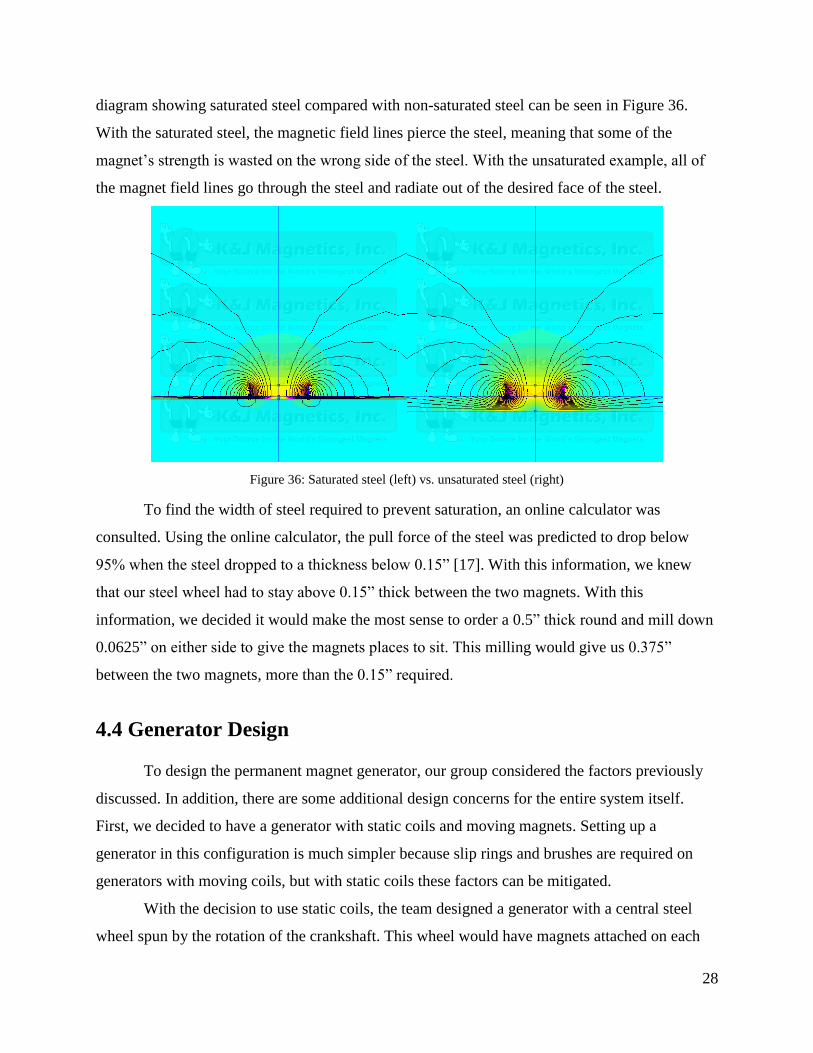
diagram showing saturated steel compared with non-saturated steel can be seen in Figure 36.
With the saturated steel, the magnetic field lines pierce the steel, meaning that some of the
magnet’s strength is wasted on the wrong side of the steel. With the unsaturated example, all of
the magnet field lines go through the steel and radiate out of the desired face of the steel.
Figure 36: Saturated steel (left) vs. unsaturated steel (right)
To find the width of steel required to prevent saturation, an online calculator was
consulted. Using the online calculator, the pull force of the steel was predicted to drop below
95% when the steel dropped to a thickness below 0.15” [17]. With this information, we knew
that our steel wheel had to stay above 0.15” thick between the two magnets. With this
information, we decided it would make the most sense to order a 0.5” thick round and mill down
0.0625” on either side to give the magnets places to sit. This milling would give us 0.375”
between the two magnets, more than the 0.15” required.
4.4 Generator Design
To design the permanent magnet generator, our group considered the factors previously
discussed. In addition, there are some additional design concerns for the entire system itself.
First, we decided to have a generator with static coils and moving magnets. Setting up a
generator in this configuration is much simpler because slip rings and brushes are required on
generators with moving coils, but with static coils these factors can be mitigated.
With the decision to use static coils, the team designed a generator with a central steel
wheel spun by the rotation of the crankshaft. This wheel would have magnets attached on each

29
side and coils suspended as close as possible next to the magnets. With this configuration, the
compression of the ramp would rotate the wheel containing the magnets. This movement induces
voltage in the coils, creating electrical power.
For a full-size version of the project, we would have a disk with 10 magnets on each side
of the wheel and two stationary wheels with 6 coils each. For the prototype, we scaled this down
to 5 magnets on each side of the wheel with 4 stationary coils on either side. A diagram of the
final design is shown in Figure 37. Initially, the group decided on 3 coils on either side of the
magnets, but while optimizing the coils we found that we would be able to fit 4 with slight
modifications to the flange diameters.
Figure 37: Diagram of generator design (measurements in inches)
4.5 Drill test
Once we finished the final set of coils, we tested the coils at higher RPM values. To test
the higher RPMs, we used the steel wheels that holds the magnets and the coils. We attached the
magnet wheel via press fit to the shaft that would turn it and attached the coil wheel with a
bearing. This meant that the magnets would spin with the shaft while the coils could be held still.
With the wheels in place, we put a single magnet on the magnet wheel and a single coil on the
coil wheel. Afterwards, we attached a drill to the end of the shaft and used the drill to rotate the
shaft at high speeds. The output voltage of the coil was measured with an oscilloscope. The

30
speed of the shaft could be solved for by measuring the time in between peaks of the
oscilloscope output. The speed was recorded as the RPM of a 6’’ diameter wheel at that speed.
The results of the testing are in Appendix E: Single Coil Drill Test.
The first tests were done with a coil that contained a steel core. The test was repeated
once with a different distance between the coil and magnet. The first test had a distance of
0.125’’. During the test it became apparent that turning the coils this close to the magnet would
be very difficult. A second test was performed with the coil and magnet 0.25’’ apart. The group
performed a third test on a coil without a steel core. The results can be seen below in Figure 38.
Figure 38: Coil test, core vs coreless
The coreless coil was much easier to spin, so we only tested it at a distance of 0.125’’ because
we were certain that the system would be able to spin 8 coreless coils.
The first test had a range of voltage values from 0.44 V at 50 RPM to 2.36 V at 384
RPM. The closest measurement to our expected 120 RPM value was 0.72 V at 116 RPM, so we
would expect 8 * 0.72 = 5.76 V from the coils at this distance with steel cores. The second test
had a range from 0.92 V at 80 RPM to 3.56 V at 379 RPM. The closest to 120 RPM was 1.52 V
at 130 RPM, leading to an expected output of 12.48 V. For the third test the range was 0.14 V at
31 RPM to 1.4 V at 375 RPM. The closest to 120 RPM was 0.472 V at 128 RPM, leading to an
expected output of 3.776 volts. The data can be seen in Appendix E: Single Coil Drill Test. The
best results were the tests with the steel cores, as expected. However, the group noticed that

31
during tests with the cores 0.125’’ from the magnet, the magnet was moving on its wheel and the
coil was getting ripped away from its wheel. In both tests with the steel cores, the system moved
irregularly because torque became much greater when the core was directly across from the
magnet. The group decided to design output circuits for the ideal steel case in case we resolved
these issues as well as for the coreless case in case these issues could not be resolved. While the
circuits were being designed, we also worked to test how much torque would be required to
move each case and which would be more reasonable to use on our final design.
4.6 Output Circuit Design
With the expected values calculated, the group designed two output circuits for the
system. Both circuits assumed the output voltage would be AC with a frequency of 8 Hz because
the both cases assumed the system would rotate at 120 RPM and RPM determines frequency.
The steel core circuit assumed a peak voltage of 12.16 volts, while the coreless circuit assumed
peak voltage of 3.776 volts.
The steel core circuit included a full wave rectifier to convert the output to a lower DC
voltage. Because the objective was to light LEDs, the lower voltage would still be high enough
to light the LEDs, while the DC waveform would keep the LEDs lit constantly. The rectifier
included a smoothing capacitor to keep the output more constant, keeping the LEDs lit. The
output of the rectifier leads directly to some LEDs connected in parallel. This configuration
allows the LEDs to share the lower voltage and be lit simultaneously. The circuit was tested in
multisim and can be seen below in Figure 39. The voltage delivered to the LEDs is shown in
Figure 40.
Figure 39: Multisim circuit

32
Figure 40: Multisim circuit LED voltage
The output changes slightly, with a peak of 2.9 V and a minimum value of 1.95 V. The
minimum value is a little below the forward voltage drop of the LEDs of 2.1 V, so for a brief
period the LEDs would dim when the system was moving. Outside of this period the LEDs
would be brightly lit.
The coreless case was much simpler. Because the voltage was not high enough to support
a full wave rectifier and still light LEDs, the LEDs were hooked directly to the output in parallel.
Half of the LEDs ran from power to ground, while the other half ran backwards, from ground to
power as seem below in Figure 41.
Figure 41: Schematic for prototype generator (coreless) output

33
The parallel alignment allowed many LEDs to share a voltage high enough to drive them.
Because they only require 10 mA of current, having many LEDs in parallel did not draw much
current from the system and the output could power them all. However, the AC output meant that
only half of the LEDs would be lit at once, with the circuit alternating between those hooked up
from power to ground and those hooked up from ground to power. Because this circuit was so
simple it was not tested in multisim.
4.7 Machining
For our generator, we are using a steel rotating wheel that has magnets mounted on both
sides which rotates within an additional two other steel wheels on either side that contain four
spools of copper wire each. The wheel with the magnets on it is 0.375” thick with 0.0625” deep
pockets for the magnets to sit in (Figure 42). The magnets are 1” in diameter, but when we
measured them the diameter was actually 1.05” so the pockets are 1.10” in diameter to allow for
removal of the magnets and to account for the slight variation in the size. The through hole in the
center is 0.5” for the rod, which is press fit to the rod which rotates, conferring torque to the
wheel.
Figure 42: Generator wheel design

34
The raw steel we are using is 1045 high strength steel that starts out 6” in diameter and is
0.5” thick. To create the final part we needed, we had to machine down the part using a VM-2
Haas machine. To create the code for the computer numerically controlled (CNC) machine, we
used Esprit to model the facing and pocketing operations that are required (Figure 43).
Figure 43: Esprit code for the generator wheel
This design, which is duplicated on both sides, uses a 0.5” ferrous end mill tool to do a
facing operation that took off 0.0625” of steel from the top, creating a flat face for the rest of the
pockets to be milled into the part. The next operation that is performed is the milling of the
recessed pockets that the magnets sit into and the through hole, which both use the same tool as
the facing operation. By taking 0.0625” off of each side of the part, the piece is milled down to
0.375” thickness. When the pocketing operation is complete, the steel between the magnets will
be 0.25” thick, which is well above the 0.1 saturation limit.
As you can from Figure 42, our original plan was to maximize the number of magnets on
the steel wheel by having 5 per side. However, as our team was mounting everything to create
the finished generator we realized that this original plan was not going to work. With five
magnets there would be a repeating pattern of n,s,n,s,n which would lead to two magnets being
the same polarity adjacent to each other which would cancel out the voltage they would each
generate. So, we modified our design to only use 4 magnets and put them at 90 degrees from
each other at the same radius as the coils so they passed directly through the center of the coils.

35
For the stationary wheels, we used the same 1045 high strength steel stock to create a
0.5” thick wheel that has four pockets. The operations are similar (Figure 44), using the 0.5”
ferrous end mill, we create the pockets for this new part.
Figure 44: Esprit file for stationary generator wheel
The wheel has only four pockets, which are 2.1” in diameter, to allow for super glue and
slight variation in the 2” diameter 3D printed part (Figure 44). The facing operation for the part
will be taking off 0.03125”, which is enough to create a smooth, finished surface, but not too
much to change the overall size of the part.
Figure 45: Stationary generator wheel

36
The pockets are 0.0625” deep, which is the depth of the flange on the coil. The coils will
then be set into these pockets. The through hole in the center is larger than the rotating generator
wheel to press fit a 1” bearing, which will allow for the rod to rotate freely.
4.8 Inertia calculations
The concept of this ramp is to be placed onto highway off ramps is that some of the
kinetic energy which is lost to heat by the brakes is recollected. Since this is the case the ramp
will be as wide as the off-ramp lane itself as seen in the following image (Figure 46).
Figure 46: Ramp location
One of the main constraints behind designing a ramp like this is the high variance in
vehicle weights. From our research we found cars could weigh anywhere from four hundred
pounds to eighty thousand pounds. Because of this high vehicle weight variance the ramp must
be able to handle the extremely high torques created by semi-trucks but also be gentle enough to
allow for a motorcyclist to pass with no discomfort.
The first thing considered in the ramp design were the springs that hold the ramp up.
Using Solidworks to create a model ramp with weight estimates we were able to calculate the
spring force required to return the one-meter long ramp to the desired ten-degree angle. The
ramp itself weighs in at about three hundred kilograms. Adding in a safety factor of 1.2 to
compensate for any extra weight give the following equations:
F=x*k
350kg*1.2*9.81m/s2=1(sin(theta))m*k

37
k=23732.9 N/m
This means that the sum of all the springs required to maintain the ramps position is
about 24,000 N/m. These springs will isolate the weight of the ramp from the calculations since
any additional load will cause the ramp to depress and the weight of the car is the only force
being added to the system.
Dividing this spring constant evenly along the ramp will ensure a sturdy result when
manufactured. Another design concern for a system such as this is being certain that a
concentrated load on only one are of the ramp will cause the entirety of it to depress. Not all
loads will be distributed evenly along the ramp so it is critical to design it such that a point force
anywhere on the ramp will cause complete depression. In order to satisfy this concern the
crankshaft must stretch along the entirety of the ramp (Figure 47).
Figure 47: Full length crankshaft requirement
In the image above one can observe the ramp in a depressed state with three separate
cranks attached to the main shaft below. Three cranks will create an even ramp depression since
the crankshaft will pull the ramp down with it even if the load is not directly above it.
Semi-trucks are another concern for a system like this. As previously stated the range of
weights traveling over this ramp is extremely large. In order to have a system that can
accommodate both extremes of this spectrum of weights there needs to be a cut off point for
maximum torque. This means we needed a component to the drive train that limits the torque
transferred to the generator. In order to protect the system from damage due to high torques we
added a torque limiter to the drivetrain similar to the one pictured in Figure 48 below.

38
Figure 48: Torque limiter
Once the torque limit is reached the device will disengage the crankshaft from the system
so that the other components are not damaged. To allow for any vehicle to pass comfortably over
this system it must also be designed with the lightest vehicles in mind. Since the springs of the
system are only enough to maintain the ramp’s height all of the resistance in the system will be a
result of the inertia of the rotating components. For this reason we had to conduct an inertia study
of the system to determine the amount of mass required for peak output via a flywheel.
To find the inertia of each individual component we first need to lay out how the
drivetrain will look on the completed system. After the torque limiter there is a flywheel and a
gearbox. The flywheel will contain an important component to the design of this ramp, a one
way-clutch. A one-way clutch allows for the output shaft to continue to rotate after the initial
input is no longer there as seen in Figure 49 below.
Figure 49: One-way clutch mechanism

39
This additional component paired with a flywheel will use the inertia of the flywheel to
keep the system spinning after a car has passed. The inertia of the flywheel will make it keep
rotating and the clutch will allow the wheel to rotate freely in order that one car passing will
create several rotations of the generator.
Having several rotations of the main shaft is critical since it will be attached to a gearbox.
A gearbox will increase the RPMs so we can spin the magnets of our generator more times to
produce more energy. For this ramp design we decided to design it with a standard off the shelf
1:10 gear ratio reduction gearbox. Table 1 lists the equipment in order of the drivetrain from the
ramp to the generator.

40
Table 1: Inertia study for full-scale ramp
Inertia
Equipment
Unit
Ratio
Unit Inertia
(kg-m2)
Ratio to
Generator
Ratio to
Ramp
at Generator
(kg-m2)
at Ramp (kg-
m2)
Ramp Iramp 1 1 10 1 0.01 1
Torque
Limiter ITL 1 0.5 10 1 0.005 0.5
Flywheel Ifw 1 100.123 10 1 1.00123 100.123
Reducer Ired 10 3.5 1 1 3.5 3.5
Generator Igen 1 0.256 1 0.1 0.256 0.00256
System
Inertia 4.77223 105.12556
Max
Acceptable 183.0050785
Difference
(%) 42.56
Torque
limiter 4000 nm s.f 1.740823816
Car Weight 2348.122521 kg 5200 lb
Smallest car 300 kg
Min Torque 511.0465869 Nm
time 0.75 s
alpha 2.792526803 rad/s2
This table shows calculations for the inertias experienced at each different components of
the system. Changing these values experimentally resulted in finding that a 100 kg-m2 flywheel
will allow for a 300kg motorcycle to pass given the g-force requirements of our background
research and still provide a 1.7 factor of safety. The governing equation for this table is as
follows:
Inertia at generator = Inertia at crankshaft / (Ratio to generator)2
The inertia for the commercial parts like the torque converter and gearbox were taken
from catalogs available on different manufacturer's websites. Components that we designed were
calculated using Solidworks. The crankshaft was designed with enough material to ensure it will

41
be strong enough to handle the max torques that are generated from semi-trucks. Below is the
information used for shaft design.
Max torque was based on an 80,000-pound vehicle traveling with a 1.2 safety factor. For
a basic low carbon steel shaft we used 167 MPa as the shear modulus which was confirmed on a
few different material property websites. Using the equation:
τ=Tc/J
In this equation, “τ” is the maximum shear stress, “T” is the applied torque, “c” is the
shaft radius, and “J” is the polar moment of inertia of the shaft. Solving with these safety factors
as constrains the minimum radius of the crankshaft should be 60cm.
The entirety of the ramp has been laid out and components have been calculated. To test
the concept we constructed a scaled prototype to test these calculations (Figure 50). This process
began with the development of a CAD model to guide us through the manufacturing process.
Below is a screenshot of a simplified CAD model for the scaled ramp model.
Figure 50: Simplified early CAD model (left) Final CAD model (right)
These three tiers are to house the entirety of the system and will be cut from acrylic.
Since the generator discs are steel and relatively heavy to be held up by acrylic we added cross
members on the sides for addition structural integrity. The picture below (Figure 51) shows the
acrylic cut for the ramp itself.

42
Figure 51: Acrylic ramp with vinyl logo
For the ramp to function correctly an additional inertia study was conducted for this size
ramp. Table 2 on the next page shows these results that we obtained from our inertia study.

43
Table 2: Inertia study for the prototype model ramp
Inertia
Equipment
Unit
Ratio
Unit Inertia
(kg-m2)
Ratio to
Generator
Ratio to
Ramp
at Generator
(kg-m2)
at Ramp (kg-
m2)
Ramp Iramp 1 0.037 10 1 0.00037 0.037
Flywheel Ifw 1 0.01 10 1 0.0001 0.01
Reducer Ired 10 0.01 1 1 0.01 0.01
Generator Igen 1 0.256 1 0.1 0.256 0.00256
System
Inertia 0.26647 0.05956
Max
Acceptable 0.2711186348
Difference
(%) 78.03
s.f 4.552025434
Smallest
car 1 kg
Min
Torque 1.703488623 Nm
time 0.5 s
alpha 6.283185307 rad/s2
In the scaled prototype, the flywheel will have an inertia of about 0.01 kg-m2 to allow for
easy operation of the ramp with just a light motion of a wrist. This gives a very large factor of
safety which results in less power out but allows for easy operation. The scaled prototype also
uses the gear for its flywheel since the gear selected has the desired inertia and the location of the
clutches allows for it to act as one.

44
4.9 Torque Estimation
Before finishing the design, it was important to estimate the torque required to turn the
wheel. The first step in estimating the required torque was to estimate the torque required to spin
the magnet wheel. The formula for mechanical torque is:
Where T is the torque, I is the inertia of the object rotating, and alpha is the angular acceleration.
Another version of this equation is:
Where omega is the final angular velocity and t is the time to reach this velocity. Because we
wanted to reach 120 RPM with a push or two, we found the final velocity of a 6-inch wheel
rotating at 120 RPM as 0.95 m/s. The time to reach this speed was estimated to be 0.5 seconds.
We calculated the inertia of our steel wheel to be 0.1 kgm2. With these numbers, the estimated
torque required to move the wheel alone was 0.019 Nm.
Next, we needed to estimate the torque required to move a ferromagnetic material inside
the magnetic field created by the magnets. To accurately calculate this force we would need to
solve Maxwell’s equations. These equations involve time consuming calculations and would
give us higher accuracy than we required. To save time, we estimated the force using a simpler
equation. The equation:
Estimates the force on a ferromagnetic material in a constant magnetic field. In this equation A is
the surface area of the object, B is the magnetic flux density acting on the object, and µ0 is the
vacuum permeability constant, equal to 4π*10^-7 H/m. The surface area of the steel cores is
.00228 m2. We found the strength of the magnetic field from the spec sheet of the magnet at ½’’
away from the magnet to be 0.0857 T. For the purpose of estimation, we assumed that the
strength of the field would be constant on the entire steel core. We used the distance of ½’’
because with steel cores we would have the surface of the core ¼’’ from the magnet and the core
was ⅝’’ high, so the middle would be about ½’’ from the magnet. Given these parameters, the
force calculated to move one of the cores through the field would be 6.656 N. For 8 coils that is
53.25 N. The centers of the cores would be 2’’ or 0.0508 m from the shaft, so we would need

45
53.25 * 0.04318 = 2.705 Nm to get the coils to move if they had steel cores and were 0.25’’ from
the magnets. The attractive force between the coil wheel and the magnets was left as 0 because
the wheel was far enough from the magnet that B became very low and the force was nearly 0.
This estimate would be larger than an experimental value because we assumed that the field
strength was constant and that each face of the cores was perpendicular to the direction of the
magnetic field. The calculated value is the total torque required to start moving the coils. This
value would be much larger than the torque required to keep it moving, so this value was the
most important to find.
These estimates showed that the main torque to overcome in our system would be caused
by the magnets. If we had no steel cores, the only torques would be the torque required to move
the coil wheel in the magnetic field and the torque to overcome the inertia of the magnet wheel.
Moreover, the fact that the torque on the cores was much higher raised concerns that our wheel
would stop spinning as soon as we stopped pushing the ramp. If we had no cores, the system
would only spin against friction, which would allow the system to get more turns from one push
on the ramp.
4.9.1 Finding Torque Experimentally
From the estimates on torque, our group saw that the steel cores and magnets may have
been too difficult for our ramp to move. Our group decided it best to test the actual torque values
of the system. To test this, our group put the shaft with the magnet wheel on two pillow blocks.
A coil wheel was put on the shaft with 4 coils attached and held in place. The coils were ¼’’
from the magnets. We cut a slot into the end of the shaft and used a torque wrench with a
flathead bit to rotate the system. Originally, we planned to measure torque with the torque
wrench, but the wrench did not get to values below 2 Nm, which was too high. To measure the
torque, we attached a spring scale to the wrench and pulled on the scale until the system turned.
Knowing the distance between the scale and the shaft gave us the distance, and the scale reading
showed us the force required to move the system. The test was run twice with a set of coils with
steel cores and one set of 4 without cores. With the steel cores, we required 5.5 N acting on a
spring scale 24 cm from the shaft, giving us 1.327 Nm of torque. Without the cores, we used 5 N
acting 12 cm from the shaft, giving us 0.6 Nm of torque. So, the experimental values showed us
that we would need 2.654 Nm to move 8 steel core coils and 1.2 Nm to move 8 coreless coils.

46
4.9.2 Removing Steel Cores
After gathering torque values, we ran another set of drill tests on the coils. The tests were
run on coil wheels with 4 coils. One wheel had the steel core coils, the other wheel had coreless
coils. The magnet wheel had 4 magnets 90º with alternating polarity. The cored coils were tested
at 0.25’’ distance from the magnets. The coreless coils were put as close as they could be without
any coils touching the magnets, a distance of about 0.0625’’. The full results are shown in
Appendix F: Four Coil Drill Test. The test closest to 120 RPM for the cored coils gave a voltage
of 4.24 V from 4 coils rotating at 195 RPM. The closest test for the coreless coils gave 2.88 V at
187.5 RPM. The output voltage of the coils connected in series did not show perfect sine waves.
The output showed 2 positive and 2 negative peaks for each full rotation. An image can be seen
in Figure 52, shown below.
Figure 52: Output voltage of 4 coils in series
The tests showed that we could expect 68% of the voltage from cored coils from coreless
coils at a closer distance. The torque required from the coreless coils was only 45.2% of the
torque required from cored coils. Additionally, the coreless coils could spin freely for a time
after a single impulse from the ramp, but coils with cores would stop after one quarter-turn if the
ramp only gave one impulse. These data showed that removing the cores would be more
effective for our push-driven prototype. For a model designed to be powered by cars, it would

47
make more sense to use a generator with steel cores and coils closer to the magnets because the
cars would provide enough force to keep the generator running smoothly from a single impulse.
After reaching this conclusion, the group removed the steel cores from the 4 coils used for
testing and began constructing the output circuit designed for the coreless coils.
4.10 Ramp prototype construction
For the non-generator components, sheets of acrylic were cut on a band saw to the
dimensions set from out CAD models and the three sheets were connected with threaded rod and
nuts. We then added our steel crossmember for additional stability and strength by cutting the
angle iron and steel flats with an angle grinder in a vice. After force fitting our magnet disc to
our shaft and sliding the coil wheels in place everything was ready for testing. Figure 53 below
shows the construction completed for testing.
Figure 53: Completed prototype
As discussed in our design selection section, a slider crank was selected for converting
the linear motion of the depressing ramp to radial motion for our generator. The components of
this crank mechanism were 3D printed due to the accessibility of the printers as well as the how
quickly we could create them. Since parts were so easy and quick to create we were able to
tweak the design of the parts for improvements. In order to translate the motion a slider crank
requires a connecting rod between the crank and slider pointed to below by the red arrow in
Figure 54.

48
Figure 54: Connecting arm
This allows for the linear motion to continue even though the crank arm moves on a
radius. However, after printing and constructing this initial design we found there were too many
losses in our design and the tolerances were not tight enough for a solid slider crank. To remedy
this we decided to get rid of the connecting rod and slot our crank arm. At this point we also
realized that the losses were not properly accounted for in our torque calculations so the torque
arm would also need to be lengthened to accommodate. Another change that had to be made was
with the springs. Since the torque required increased we decided to change the slider to have
poles pass through cup underneath to avoid any buckling as seen below.
Figure 55: New slider crank

49
In Figure 55 one can see the now increased and slotted torque arm which will still allow
for the mechanism to work as well as the anti-buckling poles for the springs. Another
improvement made to the initial construction was to add bushings for these spring poles. The 3D
printed parts had a lot of friction so adding some brass bushings to the design helped reduce this
and also allowed for more control over the tolerances which resulted in a sturdier mechanism.

50
Chapter 5. Results
Once the improvements to the ramp were finished, we assembled the generator, attached
it to the ramp, and tested the output of the full prototype. To test the output, we pushed the ramp
repeatedly to spin the wheel for a few seconds. The output from the generator was connected to
an oscilloscope and measured. Two pictures of the output from the oscilloscope is shown below
in Figure 56. The pictures are of the same waveform, with the right photograph on a shorter time
scale to show the output in greater detail.
Figure 56: Output from generator powered by hand
The output consists of sine waves of varying frequency. The frequency changing is due to
the way the generator is spun. After someone pushes the ramp, the generator spins for about 0.5
seconds. As generator slows, the frequency of the output slows. The next push speeds up the
generator again, creating a varying frequency. The peak voltages ranged from a maximum of 6.2
V to a minimum of 2.1 V. Most waveforms tended to have peaks from 4.2 V to 3 V. The root
mean squared (RMS) voltage for sine waves with these peaks is from 2.97 V to 2.12 V.
Our prototype behaved closely to our expectations. The peak voltage values within 4.2 V
and 3 V were close to our estimate of 3.776 peak voltage out for the circuit. Our group measured
the rotation of the generator using a tachometer, and the generator spun at a peak of 150 RPM
right after the ramp was pushed; above our estimate of 120 RPM. On weaker pushes, the ramp
spun at speeds ranging from 90 RPM to 131 RPM.
After we made sure the prototype was behaving properly, we assembled the output circuit
and attached it to the output of the generator. For the circuit we used the schematic described in

51
section 4.7 with 21 LEDs rather than 4. The system powered half of the LEDs at a time, with
each half alternating with the other as the ramp was pushed. Very weak pushes failed to power
the LEDs, and single pushes only powered the LEDs as long as the generator spun, about 0.5
seconds. This behavior was normal, because the LEDs were set up such that half of the LEDs
were powered by the positive portion of the AC output, and the other half were powered by the
negative portion. The LEDs did not stay on after the generator stopped spinning because a
charging capacitor cannot be used with an AC waveform.
To test the efficiency of the system, we connected the output of the generator to a 51 Ω
resistor. We ran the system with a drill and measured the power used by the drill with a plug
power meter. The drill used 43 W to run when it was running on its own at around 480 RPM.
When connected to our system, the drill used 47 W while running at the same speed. This means
that the power into our system was roughly 4 W. To calculate the output power, we measured the
voltage across the resistor as the drill was running. The output waveform can be seen below, in
Figure 57.
Figure 57: Voltage across resistor when drill powered
These measurements were taken with a different oscilloscope than previous tests. The
output showed a normal sine wave without the irregular peaks from previous tests. The output
showed peak voltages of 6.25 V. Converting from peak to RMS for sine waves is simply Vrms =
Vpk/2, giving us an RMS voltage to the resistor of 4.42 V. The output power is the total voltage
Vt. To find the total voltage, we need to account for the voltage lost in the wiring for the coils.

52
The resistance of the 8 coils was measured with a multimeter to be 11.1 Ω. With this we can find
the total voltage by treating the system as a voltage divider:
Vt = Vr(RrRr+Rc)
Where Vt is the total RMS voltage, Vr is the RMS voltage of the resistor, Rr is the resistance of
the resistor, and Rc is the resistance of the coils. With the given parameters, we measured an
output voltage of 5.38 V. The current is this total voltage divided by the total resistance, giving
us 86.7 mA. The output power is this current times the total voltage, resulting in 0.466 W.
Dividing this value by the input power of 4 W gives us an efficiency of 11.66%. The low
efficiency of the generator is mostly because the coils in the generator were coreless. If the
generators had cores, the majority of the force we put on the system would be used to overcome
the magnetic forces acting on the cores and overcoming the inertia of the steel wheel holding the
magnets would be a small portion of the force. Because we have no cores, most of the force on
our system is used to overcome the inertia of the steel wheel, and the magnetic forces between
the magnets and the wheels are only a small portion of the total energy used. This reduces our
efficiency, because most of our input power is going to inertia, rather than to the coils.
Once we finished testing the output circuit on a breadboard, we soldered the circuit on
perfboard and soldered the generator to it. The circuit can be seen below in Figure 58.
Figure 58: Output circuit of generator

53
Chapter 6. Conclusions
We created a working prototype to demonstrate our idea for a system that can both
harvest energy from braking vehicles and reduce the vehicle’s need to brake. Using a slider crank
mechanism with one-way clutches produced a ramp that always returns to its initial position and
can be actuated once and allow for several turns of the output shaft. Our generator provided
enough power for an array of LEDs to be illuminated however, the overall output of the system
is low. Since this scaled prototype required us to remove the steel cores from our coils the output
was severely reduced. One possibility to improve the output is to have a larger gear ratio since
the torque required is lower after knocking the cores out.
The next step for this project would be to build and test a full scaled prototype. Having
vehicles actuate the system will provide increased torque which will allow for the steel cores to
remain in the coils resulting in better results than our coreless coils in the scaled version.
If this project were to be continued some aspects that could be reviewed further would be
adding a transmission to the system. One of the major drawbacks of this ramp is that you must
design the loads for the lightest weight vehicle classes, motorcycles. If there were a mechanism
for detecting the weight of the oncoming vehicle and could engage/disengage a series of
flywheels one could yield far better outputs on average. This would also allow for the removal of
the torque limiter, which makes the current design act as if every vehicle that passes over it is
just a lightweight vehicle.
One other consideration that must be made is the materials selected for the ramp’s surface
itself. We would recommend in the future to have a civil engineer to review material selections
to ensure minimal wear to the system itself and the rubber of car tires.

54
References
1. Allain, Rhett. (2015). Tested: How Bright LEDs Are Compared to Other Lights. Retrieved
on October 3, 2017, from https://www.wired.com/2015/06/tested-bright-leds-compared-
lights/
2. Bartholomew, Edward. Powelka, Aimee. (2013). LED Street Lights, What is Your Plan?.
Retrieved on October 4, 2017, from http://www.mass.gov/eea/docs/doer/green-
communities/pubs-reports/led-street-lighting-slides-09-11-13.pdf
3. Boston Region Metropolitan Planning Organization. (n.d.). Average Daily Traffic on
Massachusetts Roads. Retrieved on September 28, 2017, from
http://www.ctps.org/geoserver/www/apps/adtApp/index.html
4. Brooks M., Turner H.M., Inductance of coils, University of Illinois Engineering Experiment
Station Bulletin, no. 53, 1912.
5. Central Massachusetts Regional Planning Commision. (2014). Central Massachusetts
Regional Traffic Flow. Retrieved September 28, 2017, from
http://cmrpc.org/sites/default/files/Documents/Trans/Maps/2012RegionalTrafficFlow8.5x11.
6. City of Des Moines Engineering. (n.d.). Why Can’t Speed Bumps Be Used On All Streets to
Slow Traffic? Retrieved August 30, 2017, from
http://www.dmgov.org/departments/engineering/pdf/faq9_speed_bumps_and_humps.pdf
7. Clarke R. (2010). An Introduction to the air cored coil. Retrieved on December 1, 2017 from
http://info.ee.surrey.ac.uk/Workshop/advice/coils/air_coils.html
8. Digi-Key European Editors (2012). Energy-Efficient LED Street Lights Improve Visibility,
Safety. Retrieved on October 4, 2017, from
https://www.digikey.com/en/articles/techzone/2012/may/energyefficient-led-street-lights-
improve-visibility-safety
9. Dmitriev, Victor. Electric Power Generating Speed Bump. Victor Dmitriev, assignee. Patent
US 2013/0193692 A1. 1 Aug. 2013. Print.
10. Eisele R. (2017). Calculate the intersection area of two circles. Retrieved on December 2,
2017 from https://www.xarg.org/2016/07/calculate-the-intersection-area-of-two-circles/

55
11. ElectricRate. (2017). Massachusetts Residential Electric Rates. Retrieved on October 4,
2017, from http://www.electricrate.com/residential-rates-massachusetts/
12. Empowering Pumps. (2017). AC Induction Motors vs. Permanent Magnet Synchronous
Motors. Retrieved on October 4, 2017, from http://empoweringpumps.com/ac-induction-
motors-versus-permanent-magnet-synchronous-motors-fuji/
13. Grotton, Jacob., Schramm, Christopher., Poss, Kaitlin., Evangelakos, William. (2016).
Harvesting Wasted Vehicular Kinetic Energy from Transportation Infrastructure. Retrieved
on August 15, 2017, from https://web.wpi.edu/Pubs/E-project/Available/E-project-042816-
111324/
14. Hanson, Peter. (2017). Why You Need To Know “How Much Does A Motorcycle Weigh?”
Retrieved on September 29, 2017, from http://letsridemotorbike.com/how-much-does-a-
motorcycle-weigh/
15. Hyperphysics. (n.d.) Faraday’s Law. Retrieved on September 27, 2017 from
http://hyperphysics.phy-astr.gsu.edu/hbase/electric/farlaw.html
16. Juang, Yi., Li, Shuo. (2001). Measuring and Analyzing Vehicle Position and Speed Data at
Work Zones Using Global Positioning System. Retrieved September 20, 2017, from
https://www.workzonesafety.org/files/documents/database_documents/00587.pdf
17. K&J Magnetics (n.d.). Steel Thickness Calculator. Retrieved on November 28, 2017, from
https://www.kjmagnetics.com/thickness.calculator.asp
18. Kour R, Charif A (2016). Piezoelectric Roads: Energy Harvesting Method Using
Piezoelectric Technology. Innov Ener Res 5:132. Retrieved August 29, 2017, from
https://www.omicsonline.org/open-access/piezoelectric-roads-energy-harvesting-method-
using-piezoelectrictechnology-ier-1000132.php?aid=73891
19. Kuphaldt T. (n.d.). Permeability and Saturation. Retrieved on November 28, 2017, from
https://www.allaboutcircuits.com/textbook/direct-current/chpt-14/permeability-and-
saturation/
20. Lean Engineering. (n.d.). How Does an Alternator Work? Retrieved on October 2, 2017,
from http://www.learnengineering.org/2014/04/working-of-alternator.html
21. Maurya, Akhilesh., Bokare, Prashant. (2012). Study of Deceleration Behaviour of Different
Vehicle Types. Retrieved September 15, 2017, from http://ijtte.com/uploads/2012-10-
01/5ebd8343-9b9c-b1d4IJTTE%20vol2%20no3%20(7).pdf

56
22. Meyboudi S. (2013). The Feasibility of Communication Among Pumps in a District Heating
System. Retrieved on December 12, 2017, from
https://www.researchgate.net/figure/260658571_fig11_Fig-12-Dimensions-of-a-multilayer-
coil-with-rectangular-cross-section
23. Miller-Wilson, Kate. (2014). List of Car Weights. Retrieved August 22, 2017, from
http://cars.lovetoknow.com/List_of_Car_Weights
24. MIT Science Writing and New Media. (2010). Final Report on Jerkling an Energy-saving
Speed Bump. Retrieved August 30, 2017, from https://ocw.mit.edu/courses/comparative-
media-studies-writing/21w-732-science-writing-and-new-media-fall-
2010/projects/MIT21W_732F10_jerklingrep.pdf
25. North Central Texas Council of Governments. (2014). Vehicle Types - Descriptions and
Photos. Retrieved September 20 2017, from
http://www.nctcog.org/trans/air/programs/fleet/policy/calculator/type.asp
26. U.S. Department of Transportation. (2013). Annual Vehicle Distance Traveled in Miles and
Related Data. Retrieved on September 28, 2017, from
https://www.fhwa.dot.gov/policyinformation/statistics/2013/vm1.cfm
27. Zyga, Lisa. (June 2009). Passing cars to generate energy for new UK supermarket. Retrieved
on September 26, 2017, from https://phys.org/news/2009-06-cars-energy-uk-
supermarket.html

57
Appendix A: Car Weights
Model Curb Weight
2012 Toyota Camry 3,190 pounds
2012 Toyota Prius 3,042 pounds
2012 Toyota Avalon 3,572 pounds
2013 Toyota Matrix 2,888 pounds
2013 Chevrolet Equinox
LS
3,777 pounds
2013 Chevrolet Corvette 3,208 pounds
2013 Chevrolet Malibu 3,393 pounds
2012 Chrysler Town and
Country
4,652 pounds
2012 Subaru Outback 3,495 pounds
2014 Subaru Impreza 3,208 pounds
2013 BMW 740i Sedan 4,344 pounds
2012 Honda Civic LX
Coupe
2,617 pounds
2012 Cadillac Escalade
EXT
5,949 pounds
2012 MINI Cooper
Hatchback
2.535 pounds
2013 Dodge Durango 4,756 pounds
2013 Hyundai Accent 2,396 pounds
2013 Hyundai Elantra 2,701 pounds
2012 Scion xB 3,084 pounds
2012 Scion TC 3,102 pounds
2013 Buick Regal 3,600 pounds
2014 Buick LaCrosse 3,756 pounds
2014 Buick Verano 3,300 pounds
2013 Kia Optima Hybrid 3,496 pounds
2014 Kia Cadenza 3,668 pounds
2012 Lexus IS-F 3,780 pounds
2013 Audi A6 3,682 pounds
2014 BMW 5-Series 3,814 pounds
2012 Nissan Cube 2,768 pounds
2012 Nissan Maxima 3,540 pounds
2014 Nissan Versa 2,354 pounds
2013 Ford Focus 2,935 pounds
2013 Ford Taurus 4,037 pounds
2012 Smart Fortwo 1,808 pounds
2013 Mazda MAZDA6 3,323 pounds
2014 Porsche Panamera 3,968 pounds

58
Appendix B: MATLAB Code
function [] = dynamic_ramp_remake(c, theta, m, vin, mu, k)
% c is length of ramp, theta is angle of ramp in degrees
% m is mass in kg, vin is initial velocity in m/s
% mu is ramp friction, k is the spring constant of the ramp's spring
b = c*sind(theta); % b is height of the ramp
g = 9.81; % g is acceleration due to gravity
db = b; % db is instantaneous height of ramp (this is the initial value)
dTheta = theta; %dTheta is instantaneous theta (this is inital)
dh = 0; % instantaneous height of car
% dc is the instantaneous position along the ramp
for dc = .01:.01:c
db2 = b - ((m*g*dc)./(k*c*.985)); % calculate db at this point
% check for cases where db is negative
if db2 < 0
db2 = 0;
end
dTheta2 = asind(db2./c); % calculate dTheta at this point
dh2 = dc*sind(dTheta2);
db = [db db2];
dTheta = [dTheta dTheta2];
dh = [dh dh2];
end
% loop through dh to get velocity values

59
length_dh = length(dh);
dc = 0:.01:c;
disp(length(dc))
disp(length(dh))
dv = vin; % dv is instantaneous velocity
for x = 2:1:length_dh
if dTheta(x) == 0
dv2 = ((dv(x-1).^2)+(2*g*dh(x))-(2*g*mu*.01)).^.5;
else
dv2 = ((vin.^2)+(2*g*dh(x))-((2*g*mu*dh(x))./tand(dTheta(x)))).^.5;
end
dv = [dv dv2];
end
time = [0]; % set time array, inital is 0
% Find time based on position along c
for dc=.01:.01:c;
n = int16(dc*100);
aTerm = (g./2)*sin(dTheta(n));
bTerm = dv(n);
cTerm = -dc;
poly = [aTerm bTerm cTerm];
if min(roots(poly)) < time(n)
time2 = max(roots(poly));
else
time2 = min(roots(poly));
end
time = [time time2];
end

60
dc = 0:.01:c; % define dc to allow graphing
plot(time, dv)
xlabel('Time in s')
ylabel('Velocity in m/s')
figure()
plot(time, dc)
xlabel('Time in s')
ylabel('Position along ramp in m')
figure()
plot(time, dh)
xlabel('Time in s')
ylabel('Height of car in m')
figure()
plot(time, db)
xlabel('Time in s')
ylabel('Height of end of ramp in m')
end

61
Appendix C: Pendulum test results
Test I
Trial Vmax (volts) t (ms) Speed (m/s) RPM
0 0.228 126 0.261 32.7
1 0.268 100 0.33 41
2 0.6 52 0.635 79.2
3 0.64 48 0.688 86.2
4 0.328 109 0.303 37.95
5 0.244 127 0.26 32.57
6 0.3 110 0.3 37.58
7 0.7 50 0.66 82.67
8 0.536 57 0.579 72.53
9 0.56 56 0.589 73.78
10 0.312 109 0.303 37.95
11 0.336 90 0.367 45.97
12 0.324 88 0.375 46.97
13 0.576 58 0.567 71.02
14 0.55 63 0.524 65.64
15 0.352 69 0.478 59.87
16 0.328 80 0.413 51.73
17 0.5 44 0.75 93.95
18 0.536 44 0.75 93.95
19 0.456 53 0.623 78.04

62
Test II
Trial Vmax (volts) t (ms) Speed (m/s) RPM
0 1.1 51.2 0.645 80.79
1 0.624 88 0.375 46.97
2 0.96 55 0.6 75.16
3 1.42 39.6 0.833 104.34
4 0.88 63.6 0.519 65.01
5 0.96 71 0.465 58.25
6 1.2 51 0.647 81.04
7 1.08 53 0.623 78.04
8 0.76 79 0.418 52.36
9 0.608 94 0.351 43.97

63
Appendix D: Intersection calculator code
#include <stdlib.h>
#include <stdio.h>
#include <getopt.h>
#include <string.h>
#include <unistd.h>
#include <math.h>
#define M_PI 3.14159265358979323846
#define MIN(x, y) (((x) < (y)) ? (x) : (y)) #define MAX(x, y) (((x) > (y)) ? (x) : (y))
int main(int argc, char **argv) {
double getArea(double Ar, double Ax, double Ay, double Br, double Bx, double By) { // do intersection calculation math
double d = hypot(Bx - Ax, By - Ay); // only do this math if they are intersecting
if (d < Ar + Br) { double a = Ar*Ar; double b = Br*Br; double c = sqrt((Ax-Bx)*(Ax-Bx) + (Ay-By)*(Ay-By)); double phi = (acos((b+(c*c)-a) / (2*Br*c)))*2; double theta = (acos((a+(c*c)-b) / (2*Ar*c)))*2; double area1 = 0.5*theta*a - 0.5*a*sin(theta); double area2 = 0.5*phi*b - 0.5*b*sin(phi);
if (d < fabs(Ar - Br)) { // handle cases where one circle is within the other double area = M_PI * MIN(a, b); return area; }
return area1 + area2; } return 0; }
// get input from command line
double Ar, Ax, Ay, Br, Bx, By; char x; while((x = getopt(argc, argv, "Y:y:R:r:X:x:")) != -1) // get input switch(x) {

64
case 'Y': Ay = atof(optarg); break; case 'y': By = atof(optarg); break; case 'R': Ar = atof(optarg); break; case 'r': Br = atof(optarg); break; case 'X': Ax = atof(optarg); break; case 'x': Bx = atof(optarg); break; } // open an output file for the csv
FILE *file; file = fopen("output.csv", "w"); // open file
if (file == NULL) { printf("Error, file not made properly"); return 1; } // loop through distance between circles' centers (start at max, end at 0) double distance; double division = .000542; double timePerDivision = .001; double lastArea = 0; double diffArea; double area = 0; double time = 0; Ax = 0; // make one circle stay at 0, edit other circle; Ay = 0; By = 0; // assume same height for (distance = Ar + Br; distance >= -(Ar + Br + division); distance -= division) { Bx = distance; // update 2nd circle
area = getArea(Ar, Ax, Ay, Br, Bx, By); diffArea = (area - lastArea) / timePerDivision; //if (diffArea != 0) { fprintf(file, "%f, %f, %f \n", time, area, diffArea); //}

65
// update variables
time += timePerDivision; lastArea = area; // if (By == 0) { // By+= division;/ // } else { // By-= division; // } } if (!(file == NULL)) { fclose(file); }
printf("Diff: %f\n", fabs(Ar-Br)); printf("TEST: %f\n", Ar+Br); printf("Output written to output.csv \n"); return 0; }

66
Appendix E: Single Coil Drill Test
Steel Core
1/4'' Test
Steel Core
1/8'' Test
Coreless
1/8'' Test
RPM
Peak
Voltage (V) RPM
Peak
Voltage (V) RPM
Peak
Voltage (V)
280 1.92 80 0.92 31 0.14
96 0.56 130 1.52 75 0.3
116 0.72 170 1.84 128 0.472
50 0.44 258 2.6 194 0.728
167 1 379 3.56 238 0.88
220 1.36 375 1.4
384 2.36

67
Appendix F: Four Coil Drill Test
4 Steel Core
Coils Drill Test
4 Coreless Coils
Drill Test
RPM
Peak Voltage
(V) RPM
Peak Voltage
(V)
195 4.24 187.5 2.88
329 6.16 268 4.32
681 11.6 435 7.2