Heat Transfer Effects Arising During the Linear Friction

Welding of Ti-6Al-4V

Richard Turner Roger Reed

Department of Metallurgy & Materials, University of Birmingham, UK Copyright © 2008 ITA ABSTRACT Ti-6Al-4V is the most common titanium alloy used in the aero-engine industry. In particular, it is an important material for the production of rotor blades and discs, and blisks (integrally bladed-discs). Blisks have benefits over conventional rotors, but a method of joining the two together is necessary, with linear friction welding (LFW) being one possible route. This paper considers the temperature profiles caused by frictional heating and the heat dissipation during this welding process. Thermal cycles experienced by Ti-6Al-4V were measured, by placing thermocouples close to the welded joint. The experimental results are compared with the predictions of a numerical model for the linear friction welding process. Comparison between the experimental data and the modelling is shown to be reasonable. INTRODUCTION Linear friction welding (LFW) is an important process within the aero-engine industry, particularly as it is needed to manufacture integrally joined blisks (or integrally bladed rotors) [1]. Blisks offer a significant weight reduction compared to conventional rotors, as they remove the need for heavy blade-root fixings [1]. This makes linear friction welding of blisks a desirable production method to the aero-engine industry. LFW uses linear reciprocating motion, whereby one component is rubbed across the face of a rigidly clamped mating component. This linear reciprocating motion generates a frictional heating of the two mating faces of the components, causing the material here to soften, thus providing a weld interface [2]. Axial loading applied across the weld interface causes some material to be extruded out of the weld. This is referred to as the flash. Under controlled conditions, the frictional heating can be used to join materials of an appropriate standard for structural purpose [3]. Linear friction welding is a solid-state welding process, meaning that even at the hottest section of the weld interface, the testpiece remains below its melting temperature. This adds controllability to the

process; however, knowledge of the thermal profiles of the component during production of linear friction welding would provide much greater insight into the process. It is known that only a small region of the joint, close to the weld line, will experience significant heating. In this paper, a process model for the linear friction welding of Ti-6Al-4V is described, and is used to predict factors such as thermal profiles, flash formation, stresses, strains & strain rates experienced within the joint. The experimental data gained from the thermocouples are used to validate the process model. Whilst other work has been undertaken on linear friction welding in general [4,5] and its microstructural effects [6], only very little modelling of this process has been carried out so far [7]. EXPERIMENTAL PROCEDURE Ti-6Al-4V testpieces measuring 35mm (height) x 13mm x 26 mm (mating surface) were cut from blade and disc forgings, with the same welding orientation as would have been employed when attaching a full-sized blade to the disc (Figure 1). A channel measuring 15mm deep x 12mm wide was cut through the top surface, allowing the thermocouple wires to emerge out of the fixturing surrounding the Ti-6Al-4V testpieces during processing (Figure 2). Sixteen holes were spark-eroded axially into each testpiece, with anticipated depths of 1mm, 2mm, 4mm & 8mm from the mating surface (with 4 holes cut to each depth value). The axial holes were cut into the testpiece in a 4 x 4 grid system, with columns 1, 2, 3 & 4 and with rows A, B, C & D (Figure 3). This approach allowed 4 thermocouples for each hole depth. Given the difficulties involved in producing the holes and attaching the thermocouples, 4 thermocouples set at each depth within the testpiece were considered to be enough to record the data, whilst eliminating any systematic errors and discarding outlying data from badly located thermocouples.

Figure 1: Example of a Ti-6Al-4V forged block, prior to machining and welding. The dimensions are 35mm x 26mm x 13 mm.

Figure 2: As Fig. 1, but with a 12mm deep channel machined for thermocouple wires.

Figure 3: 16 holes cut axially in to testpiece, in 4 rows and 4 columns. Holes cut to varying depths. The thermocouples were fixed into position in these holes with a chemical-set thermal cement, consistent with common practice [8]. Whilst the cement was setting, a small load was applied to the thermocouple wires to ensure that contact between wires and base of the hole was preserved. The friction-welding machine used for the experimentation joined the two testpieces one on top of the other. The top testpiece is clamped stationary, whilst the bottom one is fixed into an oscillating tooling. Once the machine has been set up correctly, the welding parameter set is entered in to the operating terminal, and the welding process takes place, with the specified oscillation frequency & amplitude and axial load applied, producing a linear friction weld (Figure 4).

Figure 4: Ti-6Al-4V welded joints with thermocouple wires attached. Different materials used to locate and attach the thermocouples, thermal cement (left) and epoxy (right). As the LFW process occurs, material is extruded into the flash from the weld line, producing an axial shortening of the testpieces. Hence, the thermocouple wires approach the weld line as the process continues. The welds considered here had an axial shortening sufficient so that the thermocouples starting closest to the weld line finished level with it. PROCESS MODELLING Process modelling has become an important tool within engineering industries as the development of computer hardware and software has improved. Nowadays, software packages are commercially available to simulate many types of metal forming processes. Linear friction welding, however, is still relatively unstudied in process modelling terms. Movement in both axial and oscillating axes (axial for the forging load, and perpendicular to this for the linearly oscillating motion – see Figure 5) make it a relatively complex process to model [7]. Any realistic model needs to be thermo-mechanical, meaning that the forces applied to the model and the temperatures being generated depend upon one another [9]. The software package Forge2007, produced by Transvalor [9], was used. Like any metal forming model, several components need to be determined to give the process model meaning, including a material model. A constitutive law is required for every deformable object within a process model. For many models including this one, the tooling (the machine parts which are in contact with the testpiece to apply the forces) are considered to be rigid bodies, and therefore do not require a constitutive law [10]. However, the testpiece itself needs to be assigned a constitutive law, which determines its deformation under the forces applied. In this work, to describe the flow behaviour of Ti-6Al-4V, a Norton-Hoff equation is used [11, 12, 13].

( TK mnmβεεσ −=

+exp3

)1(& ) ………... Equation (1)

Work previously done has established coefficients m, n, β and K used in the above equation to best represent Ti-6Al-4V. The equation for flow stress as a

function of strain, strain rate and temperature is the most accurate method of simulating the flow of the titanium alloy, however, for simplification, the model can be assumed to be independent of strain (ie: one sets the coefficient n = 0), as strain has only a small effect upon flow stress. Temperature & strain rate have been found to be the most influential factors. Boundary conditions are an important input into this process model. These are used to characterise the heat transfer coefficient of Ti-6Al-4V with the environment and the tooling. Material properties such as specific heat capacity, density and thermal expansion are defined. This model assumes an adiabatic process (no heat loss to or from the Ti-6Al-4V testpiece). The boundary conditions will also be used for mechanical boundaries to be set: - applying the load, holding the testpiece between the tooling, and to drive the oscillating motion. The LFW process model is created by producing a series of nodes, which discretize the simulation of the Ti-6Al-4V testpiece by forming a mesh. The mesh needs to be as fine as is necessary to capture the small deformations of material, and to accurately display the gradients of heat, strain & strain rate, close to the weld line. The model was created with nodes spaced apart by 0.15mm along the weld line (giving 100 nodes across the width of the testpiece) and within a window 2mm above and below the weld line. The nodes were then spaced 0.5mm apart (giving 30 nodes across the width of the testpiece) in all other regions of the testpiece. This produced a testpiece consisting of approximately 4000 elements, made up from 2000 nodes. The calculations were performed on a single CPU processor PC with 2Gb of RAM, with a run-time of approximately 50 hours.

oscillating Figure 5: Temperature fields produced by a two-dimensional linear friction weld process model.

In the work reported here, all model calculations have been performed in two dimensions. The 2D model has been assumed to be sufficient to capture the essence of the heat transfer effects occurring. Figure 5 displays an output from a 2D model, illustrating temperature profiles generated during linear friction welding.

A three-dimensional process model is more computationally expensive, with increased run-times. Work has been undertaken to produce a three-dimensional linear friction weld model. However, this model has not been used in relation to this paper. Figure 6 illustrates temperature profiles experienced in a typical three-dimensional model.

Figure 6: Temperature fields produced by a three-dimensilinear friction weld process model.

forging

Out-

RESULTS & DISCUSSION WELD PARAMETERS Three process variables relevant to linearwelding are: frequency of oscillation, amploscillation & axial forging load. These variablparameterised using a standard design of expapproach. Typical ranges of the paraconsistent with standard practice for LFW, are

• Frequency between 5 – 125 Hz • Amplitude between 0mm and the wid

testpiece (13mm in this case) • Applied forge load between 5kN –

[14]. Five values have been considered for each vwith evenly spaced increments. For the variables: (i) frequency, (ii) amplitude and (iii)forging load, the values are specified in this plow, medium-low, medium, medium-high & hithe frequency measured in Hz, amplitude min mm, and applied forge load measured in kN

forging

A full 5x5x5 matrix, including every possible parameter combination is beyond the scopeproject, so a selection of 7 parameter sechosen for the thermocouple experiments. was a control experiment, using an epoxy resthan the thermally conductive chemical set cefix the thermocouples. This parameter set wrepeated in weld 2, using the thermal cementhe thermocouples. A test matrix and subthermocouple traces from each weld can be Figures 7 to 13.

oscillating

onal

of-plane

friction itude of es were eriment meters,

:

th of the

150kN

ariable, process applied aper as gh (with easured ).

welding of this ts were Weld 1

in rather ment to as then t, to fix

sequent seen, in

Table 1: test matrix used.

Weld. no Filler material Frequency Amplitude Applied forge load

1 Epoxy Resin low medium-low medium 2 Thermal cement low medium-low medium 3 Thermal cement low medium-high high 4 Thermal cement medium-low medium-high high 5 Thermal cement medium-low high medium-low 6 Thermal cement medium low medium-high 7 Thermal cement medium medium-low medium-high

Note: Lines A1 – D4 in each of the Figures 7 to 13 represent the data (thermal cycles) recorded by the individual thermocouples, located in axial holes A1 – D4 respectively (see Figure 3), over a time period of 25 seconds, during which the testpieces were linear friction welded. Lines A1, B1, C4 and D4 correspond to thermocouples located 8mm away from the weld interface prior to welding.

Lines A2, B2, C3 and D3 correspond to thermocouples located 4mm away from the weld interface prior to welding. Lines A3, B3, C2 and D2 correspond to thermocouples located 2mm away from the weld interface prior to welding. Lines A4, B4, C1 and D1 correspond to thermocouples located 1mm away from the weld interface prior to welding.

Figure 7: Weld 1 - Temperature traces for a (low, medium-low, medium) welding parameter set. This was the control experiment, as a simple epoxy resin was used as the filler material & to locate the thermocouples.

Figure 8: Weld 2 - Temperature traces for a (low, medium-low, medium) welding parameter set using thermal cement as the filler material & to locate the thermocouples.

Figure 9: Weld 3 - Temperature traces for a (low, medium-high, high) welding parameter set, using the thermal cement.

Figure 10: Weld 4 - Temperature traces for a (medium-low, medium-high, high) welding parameter set, using the thermal cement.

Figure 11: Weld 5 - Temperature traces for a (medium-low, high, medium-low) welding parameter set, using the thermal cement.

Figure 12: Weld 6 - Temperature traces for a (medium, low, medium-high) welding parameter set, using the thermal cement.

Figure 13: Weld 7 - Temperature traces for a (medium, medium-low, medium-high) welding parameter set, using the thermal cement.

FILLER MATERIAL COMPARISON Welds 1 & 2 used the same welding parameter set, although they used differing filler materials. Weld 1 used the Omegabond ® thermal cement, whilst weld 2 used an epoxy resin, as a control experiment. The thermocouple wires located at 1mm initially from the weld interface in the epoxy resin attached experiment recorded thermal peaks of 778, 722, 753 & 710ºC (Figure 7) showing reasonable repeatability. Whereas the thermocouples located in the thermal cement attached thermocouple experiment recorded thermal peaks of 1001, 1067, 1058 & 839ºC (Figure 8). Whilst the repeatability of this trial was slightly disappointing with the one low value, this could have occurred as result of slightly incorrect hole depth, or by wire pull-out during setting of the cement. From inspection of linear friction welds carried out previously, it is apparent from the presence of certain microstructural features that material extruded as

flash from the weld line reached significantly higher temperatures than those recorded within the epoxy resin experiment, similar to those recorded by the thermal cement experiment. The reason for these low values is believed to be caused by softening of the epoxy resin at relatively low temperatures (90 - 150ºC) allowing wire pull-out during process. Further evidence of the unsuitability of the epoxy resin over the thermal cement is that the thermal conductivity of the thermal cement is 17.3 – 12.8 Wm-1K-1, whereas for a typical thermal epoxy resin, it is 1 - 4Wm-1K-1. For these reasons, the thermal cement was used as filler for the remaining five thermocouple experiments. REPEATABILITY OF EXPERIMENT The repeatability of thermocouple readings located at the same depth from the weld line in a testpiece is dependent upon accurate hole depth measurements and upon correct thermocouple location & attaching. Two examples of poorly located thermocouples can

be seen, in Weld 2 thermocouple C2, & in Weld 7 thermocouple C3. These should have been located at 2mm & 4mm from the weld interface respectively, however, the recorded values indicate that both were further than 8mm from the weld interface. Results that were significantly different from the others located at a given depth were discarded, as were assumed to be as result of poor thermocouple location. Other selected results, which displayed good repeatability of peak temperatures, are:

• Weld 3 thermocouples located 8mm from weld line (157, 147, 131, 131ºC – see Figure 9).

• Weld 3 thermocouples located 4mm from weld line (356, 328, 308, 301ºC – see Figure 9).

• Weld 5 thermocouples located 8mm from weld line (121, 129, 133ºC – see Figure 11).

• Weld 6 thermocouples located 4mm from weld line (435, 447, 486, 491ºC – see Figure 12).

• Weld 7 thermocouples located 2mm from weld line (614, 607, 604ºC – see Figure 13)

Given the far steeper thermal gradients experienced at regions close to the weld line, even small errors in

the axial hole depth or the location of the thermocouple for the wires located at 1mm and 2mm from the weld line will have a dramatic effect upon results. The results for the thermocouples located at 4mm and at 8mm from the weld line were relatively repeatable within all welds. PROCESS MODEL VALIDATION The same welding parameter sets were investigated in the Forge2007 process model, and the thermal values predicted by the model were then compared to the thermocouple readings from the experiment. Figures 14 to 19 illustrate a direct comparison of the thermal profiles seen for every weld performed using the thermal cement as the thermocouple locating material, against its modelled prediction. Figures 20 and 21 provide a three-dimensional surface, illustrating the temperatures reached as a function of their distance from the weld line and the energy input rate of the welding parameter set. Table 2 illustrates peak temperatures recorded in the thermocouple experiment and the model.

recorded peak temperature (& modelled peak temperature)

Frequency Amplitude Load 1mm T/C 2mm T/C 4mm T/C 8mm T/C Low (With epoxy)

Medium-low Medium 784ºC (1012ºC)

604ºC (701ºC)

506ºC (404ºC)

213ºC (150ºC)

Low Medium-low Medium 1036 ºC (1012ºC)

865 ºC (701ºC)

609 ºC (404ºC)

280 ºC (150ºC)

Low Medium-high

High 998ºC (1039ºC)

610ºC (718ºC)

356ºC (370ºC)

158ºC (155ºC)

Medium-low Medium High 1108ºC (1088ºC)

985ºC (875ºC)

688ºC (630ºC)

235ºC (202ºC)

Medium-low High Medium-low 1105ºC (1045ºC)

706ºC (725ºC)

364ºC (379ºC)

163ºC (175ºC)

Medium Low Medium-high

986 ºC (1026ºC)

801 ºC 707ºC)

500 ºC (403ºC)

235 ºC (160ºC)

Medium Medium-low Medium-high

1005ºC (1045 ºC)

752ºC (730 ºC)

420ºC (395 ºC)

197ºC (190 ºC)

Table 2: Comparison of thermocouple readings and model predictions. Thermocouple data has been averaged out over the 4 thermocouples at each depth, and the mean peak value recorded for each hole depth.

Figure 14: Thermal profile of weld 2, from both thermocouple data & process model.

Figure 15: Thermal profile of weld 3, from both thermocouple data & process model.

Figure 16: Thermal profile of weld 4, from both thermocouple data & process model.

Figure 17: Thermal profile of weld 5, from both thermocouple data & process model.

Figure 18: Thermal profile of weld 6, from both thermocouple data & process model.

Figure 19: Thermal profile of weld 7, from both thermocouple data & process model.

There appears to be good correlation between all thermocouple data and the modelled predictions, for every welding parameter set considered. Notably, Figure 17 illustrates a very close correlation for weld 5, and Figure 19 illustrates a very close correlation for weld 7. These experiments both had an intermediate energy input rate to the weld. THERMOCOUPLE READINGS Thermal gradients predicted by the process model for welds 2 to 7 are given in Table 3. Weld Thermo-

couple 1mm away

Thermo-couple 2mm away

Thermo-couple 4mm away

Thermo-couple 8mm away

2 320°C/mm 155°C/mm 70°C/mm 35°C/mm 3 345°C/mm 130°C/mm 55°C/mm 30°C/mm 4 205°C/mm 130°C/mm 110°C/mm 60°C/mm 5 365°C/mm 180°C/mm 50°C/mm 30°C/mm 6 295°C/mm 150°C/mm 65°C/mm 35°C/mm 7 305°C/mm 165°C/mm 50°C/mm 35°C/mm Table 3: Thermal gradients predicted in the model

Since the thermocouples record data at a fixed number of discrete points, it is difficult to draw conclusions over thermal gradients from the

experimental data. However, reasonable correlation of the temperatures at these points would imply a reasonable correlation between thermal gradients too. The highest temperatures experienced during welding will occur at the interface of the two mating surfaces, which form the weld line. The heat generated at this interface is dependent upon the mechanical energy input to the weld line via the oscillating motion. It is apparent that the work done on the mating surfaces is directly proportional to the distance that they have travelled, and to the force applied. Now, considering the distance travelled, the amplitude of oscillation (A) multiplied by 4 yields the distance travelled per oscillation. Multiplying by the frequency (f) gives the total distance travelled within one second of the process. Given that the applied load (L), frequency of oscillation (f) and amplitude of oscillation (A) are independent of one another (they are chosen as desired for the welding parameter set required) then it can be assumed that:

LAf4 Distance x Force unit time)(per doneWork ==Hence, work done (per unit time) is proportional to the product of applied load, amplitude & frequency, producing an energy input rate in units of: mm x kN x s-1 = Js-1.

To a first approximation and assuming a constant forging load, one expects the energy input to be proportional to the quantity (A x f). However, A will affect how the flash is formed, and so peak weld line temperature will not be proportional to (A x f), as the amount of input energy used to produce the flash varies. Once the affects of applied forging load are

also considered, then peak weld line temperature is definitely not proportional to amplitude x frequency. Contour plots shown in Figures 20 and 21 illustrate the relationship that the thermocouple temperatures recorded and the modelled temperatures predicted have with the energy input rate and with the distance from the weld line.

Figure 20: Three-dimensional surface, showing peak thermocouple readings as a function of distance from the weld line and effective energy input rate.

Figure 21: Three-dimensional surface, showing model prediction peak temperatures as a function of distance from the weld line and effective energy input rate.

Clearly, the results demonstrate that heat dissipation into the testpiece is dependent upon the energy input in to the weld line, the rate at which the heat is being removed via extruded material and upon the heat capacity and heat transfer coefficient of Ti-6Al-4V. Although the relationship for heat dissipation is complex, some simple rules can be derived from consideration of Figures 20 and 21. CONCLUSIONS The following conclusions can be drawn from this work: • It has proved possible to measure the thermal

profiles during the linear friction welding process. The reasonable consistency in the experimental results convinces us that the data provides a reasonable characterisation of the temperature field, for any given welding parameter set.

• Analysis of the experimental data indicates that

peak temperatures achieved during the welding process at locations close to the weld line may exceed 1100°C. Thermal gradients peaked at approximately 350°C/mm closest to the weld line.

• A process model for linear friction welding was

produced to rationalise the experimental thermocouple data. This model was based upon a Norton-Hoff constitutive equation and associated boundary conditions.

• Comparison of the experimental data and the

process model predictions indicates that the modelling is able to capture many physical aspects of the process. The thermal profiles showed good correlation with the experimental data.

ACKNOWLEDGMENTS The authors acknowledge Rolls-Royce, UK for the use of their equipment, and give thanks to Mike Rowlson, Richard March, Stan Nikov and Richard Whittaker (Rolls-Royce plc, Derby, DE24 8BJ, UK) for their expertise in the fields of linear friction welding, process modelling and titanium alloy metallurgy. The authors would like to thank Chris Bennett (University of Nottingham, UK) for the use of the data logger and for advice and technical support with thermocouple instrumentation and Dr Jean-Christophe Gebelin (University of Birmingham, UK) for help with statistical software and displaying of the results.

REFERENCES [1] S. Miller, Advanced materials mean advanced engines, Materials World Vol. 4, p446-9, (1996)

[2] A. Vairis, M. Frost, High frequency linear friction welding of a titanium alloy, WEAR Vol217, p117 - 131 (1998) [3] A. Vairis, M. Frost, On the extrusion stage of linear friction welding of Ti-6Al-4V, Materials Science & Engineering Vol.271, p477 - 484 (1998) [4] M. Karadge, M. Preuss, C. Lovell, P.J. Withers, S. Bray, Texture development in Ti–6Al–4V linear friction welds, Materials Science and Engineering: A, Volume 459, Issues 1-2, p 182-191 (2007) [5] W. Li, T.J. Ma, S.Q. Yang, Q. Xu, Y, Zhang, J.L. Li & H. Liao, Effect of friction time on flash shape and axial shortening of linear friction welded 45 steel, Materials letters Vol.62 p293 - 296 (2008) [6] C. Mary & M. Jahazi, Linear Friction welding IN718. Process Optimisation & Microstructure Evolution, Advanced Materials Research, Vol.15-17 p357-362 (2007) [7] A. Vairis, M. Frost, Modelling the linear friction welding of titanium testpieces, Materials Sci. & Engineering Vol292, p 8-17 (2000) [8] Signal Conditioning & PC-based data acquisition handbook (Chapter 6 – Temperature Measurement) – IOTech, (2008) [9] Forge2005® Training Manual – Transvalor , 2004 [10] C.C Chen & S. Kobayashi, Rigid-Plastic Finite Element Analysis of Plane-Strain Closed Die Forging, Process Modelling Fundamentals & its Applications - American Society for Metals p167-184 (1980) [11] P. Bariani, S. Bruschi & T. Dal Negro, A New Constitutive Model for Hot Forging of Steels taking into account the Thermal & Mechanical History, Annals of the CIRP, Vol.49 p195 - 198 (2000) [12] M. Vanderhasten, L. Rabet & B. Verlinden, Ti-6Al-4V: Deformation Map and modelisation of tensile behaviour, – Materials & Design, Vol. 29 p1090 -1098 (2008) [13] T. Wanheim, M. Schreiber, J. Gronbaeck, J. Danckert, Physical Modelling of Metal Forming Processes –– Process Modelling Fundamentals and Applications – American Society for Metals p145-166 (1980) [14] P. Threadgill - TWI Ltd, TWI Knowledge Summary – Linear Friction Welding (2006)

CONTACT MAIN AUTHOR Richard Turner EngD Research Student Address: Department of Metallurgy & Materials, University of Birmingham, Birmingham, UK, B15 2TT. Email: rpt988@bham.ac.uk CO AUTHOR Professor Roger Reed Director of PRISM2 Research Group Address: Department of Metallurgy & Materials, University of Birmingham, Birmingham, UK, B15 2TT. Email: r.reed@bham.ac.uk

Measuring temperature profiles during linear friction welding of Ti-during linear friction welding of Ti-

6Al-4VRichard Turner

Engineering Doctorate Research StudentDepartment of Metallurgy & MaterialsDepartment of Metallurgy & Materials

University of Birmingham, UK

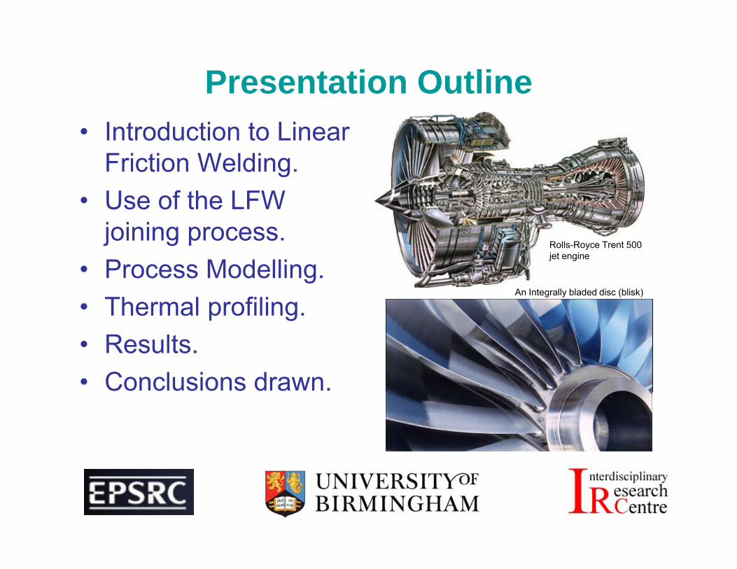
Presentation Outline• Introduction to Linear

Friction Welding.g• Use of the LFW

joining process.Rolls-Royce Trent 500

• Process Modelling.• Thermal profiling.

yjet engine

An Integrally bladed disc (blisk)

p g• Results.• Conclusions drawn.

Introduction to Linear Friction Weldingg• Solid-state process, joining similar & dissimilar materials.• Oscillating motion between parts generates frictional heating.• Minimal component distortion & high weld integrity.• Three phases of the process :

– Conditioning (Ramp-up).– Burn-off.– Forge.

• Hot layer of material extruded as “flash”.

• Axial loading applied• Axial loading applied throughout the process.

LFW Process Variables• Linear friction welding is controlled by three main variables:

– Frequency of linear oscillation (Hz).– Amplitude of linear oscillation (mm)– Amplitude of linear oscillation (mm).– Applied load (kN).

• These will govern the strength & integrity of the welded joint.• Applied load and frequency are constant throughout

process.• Amplitude is• Amplitude is

ramped up & down from

t itzero to its maximum.

Commercial Use of the Process• Blisk component within gas

turbine engines.g– LFW is one method used to

produce the Blisk.

• Weight reduction of enginesWeight reduction of engines is driving new designs:– Materials.

Blisk rather than slotted disc– Blisk rather than slotted disc.

• Blisk component can offer weight-saving of 30% over slotted disc.

Conventional Bladed Disc Integrally Bladed Disc (Blisk)

Process Modelling of LFW• Why produce an LFW process model ?

– Reduces dependence on welding trials.Eff t f i di id l t id tifi d– Effects of individual parameters identified.

– Visualise the through-process result.– However, a validation of the model is required (thermocouple data)

• Thermo-mechanical model, predicting deformation (axial shortening and flash formation) & thermal effects.

• Constitutive equation needed to represent Ti-6Al-4V flow Co s u e equa o eeded o ep ese 6 obehaviour:– :

Bo ndar conditions to define the model• Boundary conditions to define the model:– Rigid body, fixed with tooling.– Thermal properties of the material.

Modelling Animation

Flash Formation• Rippling & bifurcation can be seen in certain welds, and are

replicated within the corresponding model.

Experimental Procedurep• Ti-6Al-4V testpieces cut to 35 x 26 x 13mm blocks.• Channel cut in top surface & holes spark-eroded axially

into testpiece, to 4 varying distances:– 1mm, 2mm, 4mm and 8mm away

from weld interface• 4 thermocouples at every height –

mean values taken, ignoring any systematic errors producing outlyingsystematic errors producing outlying data.

• 7 welds performed with the thermocouples – 6 with thermal cement, 1 with epoxy filler.

Comparing thermocouple traces with modelled predictionswith modelled predictions

• A plot of temperatures recorded / predicted against welding parameters and distance from the weld.p

6000 6000

1000 1000

• Experimental data.• Modelled prediction.

1000 1000

Interpreting Results• Energy input rate α frequency x amplitude x applied load.

• Weld parameter sets with highest energy input rateWeld parameter sets with highest energy input rate predicted to have hottest weld line.

• Two conflicting mechanisms: high applied load produces g g pp phigh energy input rate, but also extrudes this hot material in to the flash faster.

• Thermocouple data accuracy sensitive to location accuracy.

• Thermocouple data showing same trend for thermal di t d l di t dgradients as model predicted.

Conclusions• It has proven possible to record LFW thermal profiles using

thermocouples with reasonable consistency.

• Thermocouple data indicates weld line temperatures exceeding 1100°C is plausible for some welding parameters.

• Thermal gradients will have an affect upon microstructure.

• Computer model to validate the thermal process also proved p p ppossible, using a relevant flow stress equation

• Comparison of thermal prediction with experimental data indicates that the model is capable of capturing the physical aspects of the process.

Acknowledgements• Many thanks to the project sponsors:

– University of Birmingham, United Kingdom.– Engineering & Physical Sciences Research Council.g g y– Armourers and Braziers, United Kingdom.– Rolls-Royce plc, United Kingdom.

• Thanks to supervisors:a s to supe so s– Professor Roger Reed (University of Birmingham).– Richard March, Stan Nikov, Mike Rowlson (Rolls-Royce).

• Thanks to colleagues for technical advice:Thanks to colleagues for technical advice:– Chris Bennett (University of Nottingham, UK).– Dr. Jean-Christophe Gebelin (University of Birmingham).

• Thanks to the ITA for this opportunity to present my workThanks to the ITA for this opportunity to present my work.

Possible future work• Process modelling:

– 3D modellingDi i il i l j i i– Dissimilar material joining

• Welding validation experiments:Welding validation experiments:– Residual Stresses (by hole drilling)– Strains (by strain gauge measurements)