heavy-duty fleet electrification
TRANSCRIPT

Page | 1
California
Heavy-Duty Fleet Electrification
Summary Report
March 2021
Prepared by

California Heavy-Duty Fleet Electrification
Summary Report
Page | 2
Authorship and Uses This report was prepared by the professional environmental consulting firm of Gladstein, Neandross & Associates (Santa Monica, CA, Irvine CA and New York City). The opinions expressed herein are those of the authors and do not necessarily reflect the polic ies and views of the project sponsor. Reference herein to any specific commercial product, process, or service by trade name, trademark, manufacturer, or otherwise, does not necessarily constitute or imply its endorsement, recommendation, or favoring by sponsoring organizations or Gladstein, Neandross & Associates. Questions regarding this report may be directed to its authors, Michael Hamilton and Patrick Couch at Gladstein, Neandross & Associates. No part of this work shall be used or reproduced by any means, electronic or mechanical, without first receiving the express written permission of Gladstein, Neandross & Associates (GNA).
Acknowledgements Preparation of this report was performed under funding by Environmental Defense Fund (EDF). GNA gratefully acknowledges the essential support of, and content contributions from, EDF. GNA gratefully acknowledges the contributions Timothy O’Connor and Pamela MacDougall at EDF. GNA also gratefully acknowledges the participation and support of NFI Industries and Schneider National, without whose participation this report would not be possible.

California Heavy-Duty Fleet Electrification
Summary Report
Page | 3
Contents 1 Executive Summary ............................................................................................................................... 5
2 Introduction .......................................................................................................................................... 8
2.1 Objective ....................................................................................................................................... 9
3 Underlying Data for Analysis ................................................................................................................. 9
3.1 NFI Chino Fleet Data Set ............................................................................................................. 10
3.2 Schneider .................................................................................................................................... 10
4 Methodology ....................................................................................................................................... 11
4.1 Parsing of Fleet Data Sets ........................................................................................................... 11
4.2 Analytical Process ....................................................................................................................... 11
4.3 Charge-Discharge Model ............................................................................................................. 11
4.3.1 Charging and Discharging Assumptions .............................................................................. 12
4.3.2 Charging Strategy ................................................................................................................ 13
4.3.3 Charger Power Rating ......................................................................................................... 13
4.3.4 Traction Battery Capacity .................................................................................................... 14
4.3.5 Modeling Scenarios ............................................................................................................. 14
4.3.6 Bad Data Handling ............................................................................................................... 14
4.4 Calculate Charge-Discharge Output Statistics............................................................................. 14
4.5 Select Baseline Scenarios ............................................................................................................ 14
4.6 Calculate Costs and Revenues .................................................................................................... 14
4.6.1 Electricity Cost Calculations ................................................................................................ 15
4.6.2 EVSE (Electric Vehicle Supply Equipment) Infrastructure Cost ........................................... 16
4.6.3 LCFS Revenue Calculation ................................................................................................... 17
4.7 Apply Optimized DER Project ...................................................................................................... 18
4.7.1 Solar PV Parameters ............................................................................................................ 18
4.7.2 Energy Storage Systems (ESS) Parameters ......................................................................... 19
4.7.3 DER Incentives ..................................................................................................................... 19
4.7.4 DER Optimization Matrix .................................................................................................... 19
4.7.5 Select Optimized DER Project Based on Net Present Value ............................................... 20
4.7.6 Rate Switch Evaluation ........................................................................................................ 20
4.8 Calculate Combined NPV ............................................................................................................ 21
4.9 Other Analysis ............................................................................................................................. 21
4.9.1 Highway vs Surface Streets Route Characterization ........................................................... 21
4.9.2 Emissions Modeling Methodology ...................................................................................... 21
5 Results ................................................................................................................................................. 22
5.1 NFI Chino ..................................................................................................................................... 22
5.1.1 Fleet Data Set Summary and Route Characterization Results ............................................ 22
5.1.2 Charge-Discharge Model Results ........................................................................................ 23
5.1.3 Selection of Baseline Scenarios ........................................................................................... 24
5.1.4 Apply Optimized DER Project .............................................................................................. 29
5.1.5 Electrification Project Combined NPV ................................................................................ 30
5.1.6 Other Analysis ..................................................................................................................... 31
5.1.7 Corridor maps ..................................................................................................................... 35
5.2 Schneider Stockton ..................................................................................................................... 36

California Heavy-Duty Fleet Electrification
Summary Report
Page | 4
5.2.1 Fleet Data Set Summary and Route Characterization Results ............................................ 36
5.2.2 Charge-Discharge Model Results ........................................................................................ 37
5.2.3 Selection of Baseline Scenarios ........................................................................................... 39
5.2.4 Calculate Baseline Costs and Revenues .............................................................................. 40
5.2.5 Apply Optimized DER Project .............................................................................................. 42
5.2.6 Electrification Project Combined NPV ................................................................................ 43
5.2.7 Other Analysis ..................................................................................................................... 44
5.2.8 Corridor maps ..................................................................................................................... 48
5.3 Results Summary and Comparison ............................................................................................. 49
5.3.1 Impact of Distributed Energy Resources ............................................................................. 49
5.3.2 Conclusions on 20 Year Combined Economics ................................................................... 50
5.3.3 Comparison to Diesel Fleet Costs ....................................................................................... 52
5.3.4 Conclusions on Capital Expenditure and Financing ............................................................ 53
6 Conclusions for Fleets and Utilities ..................................................................................................... 54
6.1 Charging Design and Management ............................................................................................. 55
6.2 Rate Options and Charging Costs ................................................................................................ 55
6.3 Conclusions on the Significance of LCFS Programs or Similar Incentives ................................... 56
6.4 Distributed Energy Resources (DERs) ......................................................................................... 56
6.5 Shared charging .......................................................................................................................... 57
7 Appendix 1 .......................................................................................................................................... 58
7.1 Trip Parsing ................................................................................................................................. 58
7.2 Charge-Discharge Model Full Statistics ....................................................................................... 59
7.2.1 Statistics Defined ................................................................................................................ 59
7.2.2 NFI Full Charge-Discharge Model Results ........................................................................... 61
7.2.3 Schneider Full Charge-Discharge Model Results ................................................................. 64

California Heavy-Duty Fleet Electrification
Summary Report
Page | 5
1 Executive Summary Deployment of medium- and heavy-duty (MD/HD) battery electric vehicles (BEVs) for commercial fleets
is accelerating. Commercial offerings of MD/HD battery-electric vehicles have increased, and medium to
large scale vehicle purchases are beginning to occur in leading fleets. At the same time, local, state and
federal policy and goal setting for zero emissions vehicle adoption is expanding.
Within the medium and heavy-duty vehicle sector, Class 8 trucks present one of the most significant
sources of emissions and have been one of the most difficult applications to electrify. These big rigs
typically have fleet specific driving schedules, long driving ranges and heavy loads. Given these challenges,
it has been unclear from a public perspective whether and how fleets that depend on these vehicles will
be able meet charging and operational demands with existing electric vehicle technology. The factors
leading to this uncertainty have involved lack of access to fleet operations data that can be used to
quantify needs, costs and operational conditions involving vehicle charging.
This study seeks to use real fleet data to evaluate the costs and capabilities of charging systems, and the
impact of electric rate design and infrastructure policy on the ability of fleets to deploy electric vehicles in
the heavy duty market segment. In doing so, the analysis seeks to enhance the body of public knowledge
on the needs and implications associated with charging systems and utility rates - as evaluated through
the lens of two separate 40 to 50 Class 8 semi-tractors deployment projects at two locations in California.
At the outset of the analysis, four issue areas were presented for analysis.
1. Fleet needs: How effective will electrification be at meeting fleet operational needs without
modification of routes and timetables?
2. Electric load: What is the aggregate and peak facility electrical load for a combination of charging
strategies, charger sizes, and traction battery capacities needed to accommodate a 40-50 heavy-
duty battery electric truck deployment project?
3. Charging rates and scenarios: Under what charging scenarios can a target facility maximize the
fraction of trips successfully charged while minimizing power demands and expected
infrastructure costs? Also, how are the costs of charging and peak load impacted by managed
charging under different electric rate variants?
4. Distributed energy resources: What role do distributed energy resources (DERs) have, including
on-site solar photovoltaic (PV) generation and battery energy storage systems (BESS), on the
charging infrastructure costs and emissions reductions profiles of each deployment? Also, how
do DER scenarios affect the aggregate facility load profile under various utility rates?
Two leading fleets in California were selected for evaluation. NFI which operates approximately 50 million
square feet of warehouse and distribution space, and its company-owned fleet consists of over 3,000
tractors and 12,500 trailers, and Schneider, a publicly-traded transportation and logistics services
company with annual revenues of nearly $5 billion, using over 9,000 tractors and 58,000 trailers and
containers. In collaboration with the fleet operators, data from daily fleet operations of 50 NFI trucks
based out of their complex of warehouses in Chino, California and 42 Schneider trucks based out of
Stockton, California were evaluated.
Using a series of sixteen separate theoretical combinations of charging power and traction battery
capacity, both the NFI and Schneider fleets were first evaluated to determine how many trips would have
been able to be successfully completed using current or advanced (announced) electric truck technology.

California Heavy-Duty Fleet Electrification
Summary Report
Page | 6
The sixteen scenarios varied traction battery capacities between 300 and 1000 kWh and charging station
power from 50 to 800 kW. Combinations of these technologies indicated that 88% of the trips performed
by Schneider’s 42 trucks and 93% of trips done by NFI’s 50 trucks over the period analyzed could
theoretically have been completed using electric trucks without modifying fleet operations. While both
scenarios rely on a not-yet-commercially-available “advanced” battery pack capacity of 1000 kWh, it is
also possible to accomplish 71% of the analyzed NFI trips using current technology on the market today.
Table 1. Summary Results for Baseline Scenarios.1
Fleet Schneider NFI NFI
Scenario Name Baseline Current Technology
Advanced Technology
DCFC Power Level (kW) 150 150 800
Truck Battery Capacity (kWh) 1,000 500 1,000
% of Successful Trips 88% 71% 93%
Maximum Number of Chargers In Use 25 40 40
Upon investigating trips which could not be completed using the traction battery and charger power
combination for each baseline scenario (failed trips), but yet were theoretically possible based on battery
capacity, it was found that most failed trips for NFI need about 70 minutes and Schneider 30 minutes or
less of additional charging (on-route) to complete successfully. This result shows that a higher charging
rate or longer charging window would significantly increase the success rate of electrified fleet trips.
Moreover, on-route charging (for example at common truck destinations such as the Ports of LA and Long
Beach) could be another way to improve successful trip coverage without the need of higher battery pack
size and charging rates. The NFI results include 5,203 failed trips compared to just 57 trips for Schnieder
that could be improved in this manner, showing that these strategies may be more impactful for certain
fleets than others, due to core operations differences between fleets.
For each of the sixteen defined charger and battery pack scenarios, the 20-year net present value of
infrastructure and electricity costs under a transition to electric trucks were evaluated. The analysis also
evaluated the impact significant of the Low Carbon Fuel Standard (LCFS) program revenues currently
offered in California. The results showed a clear positive NPV improvement using electrification when
compared to diesel fuel operations; however absent money supplied by external sources such as through
an LCFS program or government subsidy, the positive NPV improvement nearly disappears, and net costs
from charging infrastructure would not produce economically favorable electrification projects for fleets.
Programs that provide support to reduce infrastructure costs are still needed.
Furthermore, when evaluating only the annual diesel versus electricity fueling costs, excluding
infrastructure and DERs, the “fueling” costs for electric fleet are lower both in the first year as well as over
20 years showing between $4.6 and $5.8 million dollars in increased NPV compared to diesel fleet
operation. These results are shown here as Table 34.
1 For NFI, a baseline scenario with currently available technology ratings for charging and battery capacity was selected for comparison alongside an “Advanced Technology” baseline scenario with possible future technology ratings.

California Heavy-Duty Fleet Electrification
Summary Report
Page | 7
The cost of energy to charge the NFI and Schneider fleets, without the use of DERs, was evaluated using
three existing rate structures presently available in California for heavy-duty electric vehicles. The rate
structures evaluated include a commercial electric vehicle rate with a five-year demand holiday, a time of
use (TOU) rate, and an electric vehicle demand “subscription” rate. For all rates evaluated, managed
charging by the fleets is forecasted to result in significant energy cost savings over unmanaged charging.
However, due to the fleet’s operations, it was found that without DERs there was limited potential to
significantly reduce grid power demands that occurred coincident with on-peak grid periods.
Additionally, it is observed that the demand charge holiday evaluated offers significant savings in the first
5 years after deployment and becomes less economically beneficial that the standard TOU rate once the
full demand charge is reintroduced (46% of the energy costs stem from demand charges at full
imposition).
Table 2. Annual Charging Bill Calculations for Baseline Scenarios
Scenario Name Energy Demand Total Bill Rate Type
NFI Current Technology $636,364 $0 $639,424 Demand Holiday Year 1-5
NFI Current Technology $525,505 $437,338 $965,904 Demand Holiday Year 11
NFI Current Technology $350,796 $883,764 $1,237,621 TOU
NFI Current Technology $725,817 $70,964 $796,781 Demand Subscription
NFI Advanced Technology $894,433 $0 $897,493 Demand Holiday Year 1-5
NFI Advanced Technology $750,901 $973,847 $1,727,809 Demand Holiday Year 11
NFI Advanced Technology $455,963 $2,133,105 $2,592,129 TOU
NFI Advanced Technology $997,883 $158,020 $1,155,903 Demand Subscription
Schneider Baseline $912,566 $69,277 $981,843 Demand Subscription
Schneider Baseline $719,299 $977,482 $1,697,323 TOU
Schneider Baseline $797,129 $0 $800,190 Demand Holiday Year 1-5
Schneider Baseline $633,773 $426,938 $1,063,772 Demand Holiday Year 11
After application of an optimized DER project for the baseline scenarios, bill savings were calculated using
the applicable EV rate and available TOU rates for each fleet. For NFI, the demand charge holiday rate was
again found to be less advantageous than the special DER TOU rate once demand charges began phasing
in. Further, with large energy storage capabilities deployed onsite, the special DER TOU rate resulted in
the lowest energy costs, and a rate switch from the demand holiday rate to the special DER TOU rate was
recommended. For Schneider, the EV subscription rate was preferable for the life of the project including
DERs. For both Schneider and NFI, it is found that if these fleets were able to accommodate solar PV and
behind the meter BESS in their transition plans, , the savings regardless of rate subscription would make
an upfront investment of the DER resource worthwhile.
In addition to reducing charging costs for the fleets analyzed, behind the meter DER was also found to
provide a significant reduction in peak energy demand from the grid, resulting in avoided grid impacts and
savings for ratepayers if incorporated into utility grid planning. For these two fleets alone, the use of DERs
reduced the combined peak load by the order of up to 6 MW for a fleet of a little under 50 trucks. If scaled
this can result in significant savings to utilities through avoided grid buildout costs if infrastructure projects
are paired with DERs.

California Heavy-Duty Fleet Electrification
Summary Report
Page | 8
Table 3. Peak Load Reductions for Baseline Scenarios
Scenario Peak Load
Reduction (kW)
NFI Current Technology w/DER 1278
NFI Advanced Technology w/DER 4151
Schneider Baseline w/DER 611
2 Introduction Building on more than two decades of development and growth of electrification in the light-duty
passenger car market, electrification of medium- and heavy-duty (MD/HD) battery electric vehicles (BEVs)
for commercial fleets is accelerating. The number of BEVs deployed or in the process of deployment in
MD/HD fleets in the US is estimated at over 2,000 vehicles. That number is expected to double in the next
two years based on large orders placed by transit fleets as well as commercial trucking fleets, including
Amazon, PepsiCo, and FedEx. Additionally, regulations like the Advanced Clean Trucks regulation
approved by the California Air Resources Board in July of 2020 will require manufacturers to sell increasing
numbers of zero-emission commercial vehicles. A broad range of incentive programs and zero-emissions
targets set at local and regional levels across the country further incentivize the deployment of MD/HD
battery-electric vehicles.
Against this backdrop, commercial offerings of battery-electric vehicles have increased. Today, at least 21
manufactures offer more than 90 MD and HD BEV models, a substantial increase over the estimated 14
manufacturers and 50 models available for commercial sale in 2018. While most of these offerings are
currently designed for transport of people (transit, shuttle, and school buses), both new manufactures
and major manufacturers in the goods movement sector are actively developing and deploying pre-
commercial and early commercial BEVs in partnership with fleets. For example, most major Class 7/8 truck
manufacturers, including Daimler, Volvo, Peterbilt, and Kenworth, are working on heavy-heavy-duty
battery-electric trucks for near-term commercialization. These manufacturers have partnered with fleets,
such as Penske, JB Hunt, Schneider, and Dependable Highway Express, to test the integration of multiple
battery-electric trucks in real-world operations. New entrants to the Class 7/8 vehicle market include BYD,
Lion Electric, and Tesla. All are in the early stages of developing heavy-duty BEVs, while claiming to make
significant technological and/or cost breakthroughs.
With the exception of transit fleets, current deployments of MD/HD BEVs have largely been limited to a
relatively small number of vehicles at any single location. As fleets increasingly scale electrification of their
operations, concerns exist regarding the implications of increased electricity demand on both the fleet
and the electric grid. This whitepaper seeks to enhance the body of public knowledge on the needs and
implications associated with charging facilities supporting concentrations of MD/HD battery-electric
vehicle deployments at regional goods movement facilities. Specifically, this study considers the
electrification of 40 to 50 Class 8 semi-tractors at two locations in California. While facilities of this size
are common amongst major fleets, no goods movement fleet has yet deployed this many Class 8 BEVs in
a single location.

California Heavy-Duty Fleet Electrification
Summary Report
Page | 9
2.1 Objective At the outset of the analysis, four issue areas were presented for analysis.
1. Fleet needs: How effective will electrification be at meeting fleet operational needs without
modification of routes and timetables?
2. Electric load: What is the aggregate and peak facility electrical load for a combination of charging
strategies, charger sizes, and traction battery capacities needed to accommodate a 40-50 heavy-
duty battery electric truck deployment project?
3. Charging rates and scenarios: Under what charging scenarios can a target facility maximize the
fraction of trips successfully charged while minimizing power demands and expected
infrastructure costs? Also, how are the costs of charging and peak load impacted by managed
charging under different electric rate variants?
4. Distributed energy resources: What role do distributed energy resources (DER) have, including
on-site solar photovoltaic (PV) generation and battery energy storage systems (BESS), on the
charging infrastructure costs and emissions reductions profiles of each deployment? Also, how
do DER scenarios affect the aggregate facility load profile under various utility rates?
Question 1 seeks to quantify what percent of annual truck trips can be successfully met by electrification.
This requires historical analysis of current diesel fleet operations data in the context of possible electric
vehicle and charging technologies. While future electric fleet operations will surely be changed by actual
experience on the limitations of electric vehicles and charging infrastructure, this question is a
fundamental precursor to a commercial fleet’s initial decision-making to go electric. This answer speaks
to the critical issues of both range limitation as well as charging time.
Questions 2 and 3 seeks to quantify the costs and electrical impacts of charging, and how managed
charging changes these costs and electrical impacts under several typical rate variations. Unmanaged
charging will be used as a baseline for comparison representing what is expected to be the worst-scenario
outcome for charging cost and peak electrical load. Managed charging is expected to, by design, change
the electric load profiles to reduce charging cost and peak electrical load, and will be compared to the
unmanaged charging baseline. By looking at several typical rate variations both specific to EVs and non-
EV commercial/industrial rates, a range of potential charging costs can be determined.
Question 3 seeks to characterize the impacts of DERs on charging costs and peak electrical load. Solar PV
is expected to offset electrical load during daytime hours and energy storage is expected to store any
excess PV to reduce peak loads and offset any remaining on-peak charging energy. Optimizing the size of
solar PV and energy storage can yield cost-effective reductions to charging costs and peak load. These
results for charging costs and peak load for optimized DER combinations will be evaluated under different
rate variations.
3 Underlying Data for Analysis The datasets forming the basis of this white paper reflect twelve months of real-world truck activity data
provided by two leading for-hire/logistics fleets, NFI and Schneider. These companies are two of the
largest for-hire motor carriers in the US, operating a combined 13,000+ Class 7 and Class 8 semi-tractors

California Heavy-Duty Fleet Electrification
Summary Report
Page | 10
nationally. Over 1.4 million Class 7-8 trucks like those in the current study operate in California, travelling
44 million miles per day on California roads.2
NFI is a fully integrated third-party supply chain solutions provider headquartered in Camden, New Jersey.
NFI business lines include dedicated transportation, warehousing, intermodal, brokerage, transportation
management, global, and real estate services. Privately held by the Brown family since its inception in
1932, NFI generates more than $2 billion in annual revenue and employs more than 13,100 associates.
NFI operates approximately 50 million square feet of warehouse and distribution space, and its company-
owned fleet consists of over 3,000 tractors and 12,500 trailers. 3
Schneider is a publicly-traded transportation and logistics services company headquartered in Green Bay,
Wisconsin. Schneider offers tailored dry van truckload, intermodal, bulk and dedicated trucking solutions.
Schneider has annual revenues of nearly $5 billion, employs or contracts with over 15,000 people, using
over 9,000 tractors and 58,000 trailers and containers.
The two California fleets both represent return-to-base operations, which allow for a central charging
depot operations design. Both fleets operate nationally covering a wide range of good movement
activities from major hubs such as ports and rail terminals, to intermediate destinations such as
warehousing, storage, and distribution facilities, and finally to end customers.
3.1 NFI Chino Fleet Data Set NFI’s provided a data set for their drayage trucking fleet based out of their complex of warehouses in
Chino, California. The primary activity of this fleet is shipping container movement to and from the San
Pedro Bay Ports (the combined Port of Los Angeles and Port of Long Beach) as well as between Chino and
various NFI customer destinations in Southern California. Additionally, there are some long-distance and
out-of-state destinations included, but these occur infrequently. There are plans for future electrification
of the Chino fleet, thus adding practical importance to the results of this analysis.
The data set includes raw GPS telematics data and driver performance system data covering the 2019
calendar year. This included about 1 million GPS records and 500,000 records from the driver
performance system. In its raw form, it included data on 57 vehicles, but after removing vehicles that did
not have complete data or were not representative of normal operations, 50 vehicles remained. These
trucks are assumed to be equipped with emissions control equipment that is typical of their vintage per
minimum California requirements. No near-zero-emissions (NZE) vehicles are known to be part of this
fleet.
3.2 Schneider Schneider provided a data set for their trucking fleet based out of Stockton, California. The primary
activity of this fleet is shipping container drayage movement to and from the BNSF Stockton railyard as
well as between various Schneider customer destinations in Northern and Central California. Additionally,
there are some long-distance and out-of-state destinations included, but these occur infrequently.
The data set includes trip dispatch data and fueling data from September 2019 to September 2020. This
included about 80,000 trip records and about 23,000 fueling records. A total of 42 vehicles used in local
2 California Air Resources Board, 2019 Annual Enforcement Report, Table I-7, https://ww2.arb.ca.gov/sites/default/files/2020-06/2019_Annual_Enforcement_Report.pdf 3 NFI Website About Us. https://www.nfiindustries.com/about-nfi/

California Heavy-Duty Fleet Electrification
Summary Report
Page | 11
goods movement activities were included in this analysis. These trucks are assumed to be equipped with
emissions control equipment that is typical of their vintage per minimum California requirements. No
near zero emissions (NZE) vehicles are known to be part of this fleet.
4 Methodology
4.1 Parsing of Fleet Data Sets Data sets were developed for each fleet using the GPS and operational source data to characterize both
the round trips and charging windows (times when the truck is at the home depot and available for
charging) for each truck over a complete one-year period. These data sets form the basis for the
subsequent analysis of charging loads, utility costs, and infrastructure requirements.
4.2 Analytical Process These fleet data sets are then analyzed under a multistep process:
1. Apply the charge-discharge model to determine the aggregate facility electrical load profile for
each input scenario of charging strategy, charger rating, and traction battery capacity.
2. Calculate statistics for electrical load and successful trip coverage
3. Select baseline charging scenarios for further analysis based on inspection of successful trip
coverage, electrical loads, and technology availability
4. Calculate baseline costs and revenues including electricity costs under various utility rates, and
estimates of charging infrastructure costs and LCFS revenues
5. Size an optimized DER project for each selected scenario including on-site solar photovoltaic (PV)
generation and battery energy storage systems (BESS) to minimizing charging costs and peak
electrical loads
6. Calculate combined net present value (NPV) including DER project, electricity costs, infrastructure
costs, and LCFS revenues
The process is presented visually in Figure 1.
Figure 1. Analytical Process
Additionally, several other analyses were also performed including emissions calculations, highway vs. on-
street route characterization, as well as freight corridor analysis.
4.3 Charge-Discharge Model A charge-discharge model was developed to convert the one year set of fleet trips and charging windows
into an aggregate electric load profile for each fleet. At a high level, the round trip distance determines
the energy discharge and ending state of charge (SOC) of each round trip. Upon arrival at the depot, the
EV charging demand is determined by this SOC and the available charging window between vehicle arrival
at the depot and the next time of departure from the depot. The truck charges, then leaves on the next
round trip, and the cycle continues for the entire one-year period.

California Heavy-Duty Fleet Electrification
Summary Report
Page | 12
This charging model treats every truck and charger independently, and thus the aggregate facility results
are the sum of each truck’s independent charging profile. This study does not explore optimization of
charger sharing or multi-plug charger cascading.
The following inputs to the model were selected using a range of scenarios to explore a range of
technologies and charging assumptions:
• Charging strategy
• Charger power rating
• Traction battery capacity
4.3.1 Charging and Discharging Assumptions Several assumptions are made as part of the charge-discharge model.
Energy Economy: Energy economy, defined in units of kWh per mile, is assumed to be constant for all
trips within a given fleet. Energy economy is multiplied by the round trip distance to determine the total
energy consumed and therefore discharged by the battery during the round trip. This allows calculation
of the corresponding SOC percent.
Each fleet provided estimated energy economy based on field experience and discussions with
manufacturers. NFI estimates energy economy at 2.0 kWh/mi while Schneider suggested a value of 2.4
kWh/mi. These values can vary widely based on vehicle loading, driver patterns, and the type of routes
being travelled.
Charging Efficiency: Efficiency from the utility meter to the DC charging plug is assumed to be 95%. Battery
charging efficiency is assumed to be 92.5%, resulting in a combined net charging efficiency of 87.88% from
the Alternating Current (AC) grid supply to stored Direct Current (DC) energy in the battery pack. Actual
values may vary based on charger, charge rate, battery type, and battery management system design.
However, the assumed overall charging efficiency is similar to the range of efficiencies reported by the
California Air Resources Board.4
Charge Rate Limiting: To protect the battery, the charging rate for EV batteries must be tapered down as
the battery reaches a high state of charge. To characterize this behavior, a simple battery C-Rate limit
model was applied5. This model limits the charge rating to be less than or equal the C Rate Limit when
the state of charge (SOC) is between certain threshold values.
4 California Air Resources Board, “Appendix H: Analysis Supporting the Addition or Revision of Energy Economy Ratio Values for the Proposed LCFS Amendments,” March 6, 2018. https://ww3.arb.ca.gov/regact/2018/lcfs18/apph.pdf. 5 The assumed charge tapering profile in this study is consistent with at least one powertrain manufacturer's approach known to GNA. Other manufacturers may implement more or less aggressive tapering schedules, which will impact total charging time.

California Heavy-Duty Fleet Electrification
Summary Report
Page | 13
Table 4. C Rate Limit as a function of SOC Threshold
SOC Threshold C Rate Limit
0% 1
90% 1
92% 0.5
94% 0.25
96% 0.125
98% 0.0625
100% 0.03125
4.3.2 Charging Strategy Charging strategies were defined for unmanaged and managed charging. Each strategy defines the core
algorithm logic about how fast and at what times the vehicle charges during each available charging
window.
4.3.2.1 Unmanaged Charging
This strategy assumes full speed charging, subject to the charging assumptions described below, at any
time, with no attempt to manage charging by time of use (TOU) period or minimize peak power demands.
The trucks will charge as fast as possible, immediately, anytime.
4.3.2.2 Managed Charging
This strategy assumes both (1) the charge timing can be adjusted to avoid peak TOU periods, provided
this adjustment does not prevent the truck from fully charging before departure and (2) charging power
is reduced to the minimum required to fully charge the battery within the available depot charging
window.
Charge Timing: The algorithm initially scans the electricity rate definition to extract information about the
timing of the peak TOU periods. Next, the available depot charging window is compared to this peak TOU
period information. If there is an opportunity to charge before or after the TOU window, while still
allowing a full charge, an adjustment to the charging schedule is made. If adjusting the charge would
result in only a partial charge possibility, then this algorithm will force charging in the peak TOU window.
Charging Power: If reducing the charge power would prevent the truck from fully charging before
departure, then this algorithm will force charging at full power as needed. This algorithm actively solves
for the optimal charging power based on the available charge window, so the vehicle will complete
charging just before needing to depart on the next round trip.
This managed charging approach achieves the goal of both minimizing peak power demand as well as
shifting charge times to avoid peak TOU periods.
4.3.3 Charger Power Rating For this study, the vehicle charger selection is based on direct current (DC) fast charging technology.
Scenarios for charger power ratings were defined to represent current and future technology options.
This scenario range includes 50 kW, 150 kW, 350 kW, and 800 kW6. The 50kW and 150 kW options are
widely available products today. The 350 kW product has some commercial availability using liquid-cooled
6 all DC ratings

California Heavy-Duty Fleet Electrification
Summary Report
Page | 14
cables or an overhead pantograph connection. The 800 kW charger is a speculative product representing
a rating implied by claims made by Tesla regarding the recharging times for its Semi.
4.3.4 Traction Battery Capacity Scenarios were defined to include four different traction battery pack sizes of 300, 500, 750, and 1000
kWh. This rating is modeled as usable DC capacity, intended for 0 to 100% SOC operation. The 500 kWh
rating is similar to several early commercial truck options, and the 1000 kWh rating is a speculative rating
representing the 500-mile range Tesla Semi. The 300 kWh and 750 kWh ratings are included for
comparison of a wider range of vehicle battery capacities.
4.3.5 Modeling Scenarios In total for each fleet, 32 scenarios were modeled, which represent all possible combinations of the two
charging strategies, four DC fast charger ratings, and four battery pack ratings.
• Charging Strategy: Unmanaged and Managed
• Charger Power Rating: 50 kW, 150 kW, 350 kW, and 800 kW
• Traction Battery Capacity: 300, 500, 750, and 1000 kWh
4.3.6 Bad Data Handling The charge-discharge model inspects for “bad data” and excludes these data points from inclusion in the
analysis. This bad data originates from errors in the source data set that such as incorrect timestamps
and ECM odometer values. The errors were flagged so any affected trips or charging windows would be
skipped in the charge-discharge model. Examples of such errors were:
• negative values for charge window time
• negative values for trip distance
• unrealistically high average speeds
• charging window stop time misalignment with round-trip start time
• round trip stop time misalignment with charging window start time
4.4 Calculate Charge-Discharge Output Statistics In addition to generating the aggregate charging load profile of 15-minute data, several statistics were
calculated for each model scenario. This included core electrical statistics regarding the maximum
number of chargers utilized, electricity consumption, and peak load. Additionally, statistics were
calculated to characterize the percent of total trips that were successfully completed, excluding the trips
that were skipped. Full definitions of these statistics are provided in the Appendix Section 7.2.1.
4.5 Select Baseline Scenarios Baseline scenarios were selected for further analysis based on inspection of a variety of factors including
successful trip coverage, electrical loads, and technology availability. This flexible approach was used to
allow focus on the most relevant scenarios for both NFI and Schneider fleets for the remaining analysis.
4.6 Calculate Costs and Revenues For the selected baseline scenarios, several costs and revenue calculations were made including
electricity costs, infrastructure costs, and LCFS credit revenues.

California Heavy-Duty Fleet Electrification
Summary Report
Page | 15
4.6.1 Electricity Cost Calculations Four different rate categories were utilized in this calculation to represent a range of options relevant to
commercial EV fleets.7
1. Demand Holiday – This rate is an EV incentive rate that has no demand charges to lower total
costs for early EV adopters. The rate contains Time of Use (TOU) energy charges, and though
demand charges are re-introduced over time, they remain low compared to the TOU Commercial
rate.
• Demand Subscription – This rate is an EV-specific rate that has demand charges billed in pre-
selected subscription blocks, to reduce uncertainty about demand charges for early EV adopters.
The rate has higher energy charges, and though demand charges are present, they remain low
compared to the TOU rate. Overages on demand above the pre-paid demand blocks are charged
at a higher rate.
2. TOU Commercial– This rate is the typical commercial/industrial time of use rate that would
normally apply had the customer not sought a demand holiday or subscription EV rate. The TOU
rate typically has high demand charges and lower energy charges compared to the demand
holiday and subscription EV rates, as well as compared to the Special DER rate.
3. Special DER – This rate is only available for sites with DER projects including PV or energy storage,
and typically has low demand charges and high energy charges, which can allow for lower total
bills when using DERs.
An electricity billing calculation engine was created to accurately estimate electric bills for these rate
categories. Note these are all assuming medium voltage or transformer “primary” metering, which will
be typical for installs larger than ~2 MW in total charger rating that exceed typical secondary service
standards.
For NFI, the following rates were evaluated:
• Demand Holiday – SCE TOU-EV-9 for 2 to 50kV – This is the actual EV rate available for a potential
NFI electrification project. Both the initial rate with no demand charge and the final rate with full
demand charge will be evaluated.89
• TOU – SCE TOU-8-D for 2 to 50kV – This is the typical commercial rate for SCE customers in this
size range with peak periods of 4 to 9pm.10
• Demand Subscription - BEV-2-P for Primary Voltage – While not actually available for NFI, this rate
is useful for comparison. For this modeling, the demand subscription blocks are approximated as
7 More information can be found in the EDF “SMART PRICING PRINCIPLES FOR CHARGING ELECTRIC TRUCKS AND BUSES” at http://blogs.edf.org/energyexchange/files/2020/10/ChargingFactSheet.pdf 8 Southern California Edison, https://library.sce.com/content/dam/sce-doclib/public/regulatory/tariff/electric/schedules/general-service-&-industrial-rates/ELECTRIC_SCHEDULES_TOU-EV-9.pdf, Accessed September 2020 and active on June 1, 2020. 9 SCE EV-9 demand charge re-introduction schedule from year 6 to 11 was provided from SCE by email correspondence on July 31st, 2020 10 Southern California Edison, https://library.sce.com/content/dam/sce-doclib/public/regulatory/tariff/electric/schedules/general-service-&-industrial-rates/ELECTRIC_SCHEDULES_TOU-8.pdf . Accessed on September 2020 and active on June 1, 2020.

California Heavy-Duty Fleet Electrification
Summary Report
Page | 16
a simple monthly per kW demand charge, which is a reasonable approximation of future bills
when assuming no demand overages.11
• Special DER – SCE TOU-8-E for 2 to 50kV – This is the DER rate for SCE customers in this size range
with peak periods of 4 to 9pm. This rate will be evaluated during the DER project analysis section.10
For Schneider, the following rates were evaluated:
• Demand Subscription – PG&E BEV-2-P for Primary Voltage – For this modeling, the demand
subscription blocks are approximated as a simple monthly per kW demand charge, which is a
reasonable approximation of future bills when assuming no demand overages.11
• TOU - PG&E B-20 for Primary Voltage – This is the typical commercial rate for customers in this
size range. This is a high demand charge and lower energy charge TOU rate with peak periods of
4 to 9pm. This rate is opt-in only today, but will become default over the next two years, so is
considered the best assumption for a typical commercial rate on this project.12
• Demand Holiday – SCE TOU-EV-9 for 2 to 50kV – While this is not available for a potential
Schneider electrification project in PG&E territory, this rate is useful for comparison. Both the
initial rate with no demand charge and the final rate with full demand charge will be evaluated.89
• Special DER - PG&E B-20 Option R for Primary Voltage – This is a special rate available only to
customers with DERs such as PV or energy storage. This rate has high energy charges, and lower
demand charges, which can make it favorable for DER projects.12
For each rate, the non-bypassible energy charges13 are separated to allow accurate assessment of solar
PV generation with net energy metering (NEM) successor rate rules.
For each rate, a manual assessment of which TOU periods should be considered “Peak” for purposes of
the charging algorithm was applied. For example, if mid-peak naming is used for the 4-9pm peak in the
winter, this is considered “peak” for purposes of the charging algorithm.
4.6.2 EVSE (Electric Vehicle Supply Equipment) Infrastructure Cost EVSE Infrastructure costs were estimated including chargers and associated electrical infrastructure for
each baseline scenario. These estimates were created using GNA’s best estimates of current costs for the
California market according to actual project experience in 2019 and 2020. Purchase costs for the EVSE
are based on publicly available cost information from a recent state procurement process.14
Site work costs, including switchboard and transformer upgrades, are estimated for the total number of
chargers in each Scenario and then levelized on a per-charger basis. The combination of the Total Installed
Cost per Charger and the Site Work Cost per Charger can then be approximated as a Total Scenario Cost
per Charger.
11 Pacific Gas and Electric, https://www.pge.com/tariffs/assets/pdf/tariffbook/ELEC_SCHEDS_BEV.pdf. Accessed September 2020, and active on May 1, 2020 12 Pacific Gas and Electric, https://www.pge.com/tariffs/assets/pdf/tariffbook/ELEC_SCHEDS_B-20.pdf. Accessed September 2020, and active on May 1, 2020 13 These are charges defined by the CA CPUC that must be paid, despite excess PV being allowed to reduce the remaining energy charges via NEM. 14 State of Ohio Department of Administrative Services, “Invitation to Bid: Electric Vehicle Chargers and Equipment”, Bid #: RS900320, September 2019.

California Heavy-Duty Fleet Electrification
Summary Report
Page | 17
Additionally, a value for estimated charger system operation and maintenance (O&M) has been estimated
in terms of $/year. A 3% per year escalator is applied for this O&M estimate when extended for use in
the 20-year project financial model.
4.6.3 LCFS Revenue Calculation Both sites are in California and can generate credits under California’s Low Carbon Fuel Standard (LCFS)
program. The credits can be sold to generate significant revenues that can be used to offset electricity
costs and infrastructure investments. LCFS revenue calculations were made using the following
assumptions:
• A fixed $200/credit price over the 20-year modeling period, consistent with current market
pricing.15 Note that the LCFS program recently implemented a cap on credit prices, limiting the
sale price of credits to $200, adjusted by the consumer price index with a baseline year of 2016.
Currently, the effective cap on credit prices is approximately $218.
• Diesel fuel carbon intensities (CIs), energy economy ratios, and benchmark CIs for heavy-duty
vehicles reflect values in the currently adopted LCFS Regulation.
• Carbon intensities (CIs):
o Grid-supplied electricity: Values are projected based on 2020 grid carbon intensity as
reported by the LCFS program. Year-over-year percentage reductions in GHG emissions
expected from Senate Bill 35016 are then applied to the baseline 2020 grid carbon
intensity to forecast grid carbon intensities through 2030, with the results shown below
as Table 5. The grid CI for years 11 to 20 use the same value as 2030.
o On-site solar PV generation: Electricity supplied by on-site solar PV generation is
assigned a carbon intensity of zero.
o Smart charging pathway: The CIs listed in
o Table 6 are utilized to calculate the aggregate CI based on the actual time of charging 17.
These CIs represent GHG emissions by hour of day and by calendar quarter for California
grid-average electricity.
Any electrical demands not met by on-site solar PV generation are assumed to be served by grid-average
electricity.
Table 5. Grid Carbon Intensity (gCO2e/MJ) Assumptions
Year 2020 2021 2022 2023 2024 2025 2026 2027 2028 2029 2030+
Grid CI 82.92 81.63 78.67 74.19 66.88 59.95 55.91 51.28 46.23 40.96 34.02
15 Pricing may increase or decrease in future due to a wide variety of factors. While the program becomes more stringent over time, providing upward pressure on prices, a number of new fuel production facilities are proposed or in development that could provide new credit supplies that would place downward pressure on prices. We do not attempt to forecast prices in this study. 16 California Energy Commission, 2018 IEPR Update, Volume II. https://ww2.energy.ca.gov/2018publications/CEC-100-2018-001/CEC-100-2018-001-V2-CMF.pdf 17 California Air Resources Board, “2020 CARB LOW CARBON FUEL STANDARD ANNUAL UPDATES TO LOOKUP TABLE PATHWAYS: California Average Grid Electricity Used as a Transportation Fuel in California and Electricity Supplied under the Smart Charging or Smart Electrolysis Provision”, January 8, 2020.

California Heavy-Duty Fleet Electrification
Summary Report
Page | 18
Table 6. Smart Charging Carbon Intensities (g CO2e/MJ) for 2020
Hour Starting Q1 Q2 Q3 Q4
12:00 AM 80.41 80.41 81.33 83.96
1:00 AM 80.41 80.28 80.19 81.82
2:00 AM 80.41 79.35 80.14 80.99
3:00 AM 80.41 80.55 80.12 80.84
4:00 AM 80.41 80.38 80.09 81.8
5:00 AM 82 84.17 80.29 89.17
6:00 AM 98.41 96.98 87.77 109.9
7:00 AM 104.82 67.86 84.52 107.45
8:00 AM 76.88 2.24 81.5 88.44
9:00 AM 53.96 1.63 56.55 83.29
10:00 AM 53.17 2.43 58.89 55.67
11:00 AM 51.95 46.3 64.8 58.91
12:00 PM 27.3 49.1 72.69 60.26
1:00 PM 27.3 50.8 83.29 84.98
2:00 PM 52.06 54.05 90.27 86.4
3:00 PM 53.27 58.5 106.12 93.52
4:00 PM 65.1 24.38 112.3 115.8
5:00 PM 106.97 29.38 120.4 138.98
6:00 PM 124.44 98.7 134 140.88
7:00 PM 120.98 139.24 143.4 134.74
8:00 PM 110.01 138.55 128.41 124.81
9:00 PM 92.22 112.15 108.21 110.57
10:00 PM 81.84 85.84 91.66 97.45
11:00 PM 80.41 81.22 83.62 86.71
4.7 Apply Optimized DER Project A procedure for determining an optimized DER project for a given vehicle load profile can be used here
to estimate a cost-effective DER project for each baseline scenario. There are many ways to size DER
projects, and this method is only one way to determine an optimum combination of solar PV and energy
storage.
4.7.1 Solar PV Parameters The maximum size for solar PV was estimated as the solar array size generating approximately 80% of
annual energy consumption. This is a best practice for sales engineering in the combined solar PV and
storage industry.18 as solar PV sizes approaching higher than 80% of annual consumption tend to reduce
the relative value of energy storage, by eliminating the chance for significant TOU energy arbitrage using
the battery, which is due to CA NEM rules. For example, start with an arbitrary annual energy
consumption of 6,750,000 kWh. Using 80% of this value, and assuming 1500 kWh annual generation per
18 These assumptions for solar PV and energy storage sizing are “rule of thumb” approximations from GNA professional experience in the commercial energy storage and solar PV business.

California Heavy-Duty Fleet Electrification
Summary Report
Page | 19
kW DC of Solar PV, this yields a solar PV size of about 6,750,000 kWh * 80% / (1500 kWh/kW) = 3600 kW
DC for the maximum PV sizing. A second size of about half this amount and a scenario with no solar PV
were also evaluated for comparison
For solar PV installed pricing, both a “low-cost PV” scenario at $2/W scenario and “high-cost PV” scenario
at $5/kW was used18. The low-cost PV is representative of a moderately priced rooftop PV installation,
and the latter of dedicated, canopy-supported PV system installation. These prices are representative of
the current market for solar PV technology, but actual site installed costs will vary widely. Since there are
no actual sites for electrification selected by either fleet, no site-specific solar PV analysis was performed
in this study.
Maintenance costs for solar PV use a rough approximation of 1.5 cents per watt DC per year is used. This
is a common O&M allocation for commercial PV project development. Annual degradation of PV
generation performance is assumed to be 0.5% per year, not compounded. Inverter replacement costs
are applied in year 11, assumed as 6.5 cents per watt DC PV rating.18
4.7.2 Energy Storage Systems (ESS) Parameters Energy storage system (ESS) sizing was based on kW ratings less than or equal to the size range of the PV
DC nameplate rating, for 2-hour and 4-hour durations, which are the most common available products
today.18 Following the same example above with a PV rating of 3600 kW PV, an ESS Power rating of 2500
or 3000 kW was selected as the maximum size considered. Using 2500 kW gives 2500 kW / 5000 kWh
and 2500 kW / 10000 kWh for the 2-hour and 4-hour options, respectively. Two additional ESS system
sizes based on half of the maximum power rating for 2-hour and 4-hour durations were evaluated for
comparison. The scenario of no ESS was also evaluated.
For ESS installed pricing and annual O&M, linear regression models were developed using real 2019
California installed price estimates from a major commercial DER developer. Annual performance
degradation of ESS is assumed to be 2% per year, not compounded. A battery augmentation cost
allocation of $200/kWh for 20% of capacity, and inverter replacement cost allocation of $100/kW are
applied in year 11 based on typical industry practice for maintenance of ESS performance.18
4.7.3 DER Incentives For “Solar PV Only” or “Solar PV and ESS” projects, the Federal Investment Tax Credit (ITC) is available and
is currently in 2020 crediting 26% of eligible project capital costs, which includes the entire PV and storage
capital costs as basis. Note the solar PV ITC incentive declines each year and will become much less
valuable after 2023 when it declines to 10% permanently.
Since these are California locations, the Self Generation Incentive Program (SGIP) is available for
commercial energy storage projects, and this incentive is included in the DER modeling using Step 3
program assumptions valid in September 2020 for both PG&E and SCE territory. This total incentive is
adjusted lower when present on a solar PV and ESS project that is taking Federal ITC as well.
4.7.4 DER Optimization Matrix An initial search matrix was generated based on combinations of solar PV, ESS, and utility rate
assumptions for each location, as summarized in Table 7. In total 90 scenarios per charging scenario and
location were evaluated: 3 PV sizes x 2 PV Prices x 5 ESS sizes x 3 rates. ESS prices were not varied as part

California Heavy-Duty Fleet Electrification
Summary Report
Page | 20
of the matrix of scenarios since they do not widely vary based on site situation in the way that solar does
for rooftop vs. carport.
Table 7. Parameters used to develop the DER Optimization Matrix
Location PV Array Sizes PV Price ESS Sizes Utility Rates
NFI None 1,250 kW 2,500 kW
$2 per watt $5 per watt
None 1,250 kW / 2,500 kWh 1,250 kW / 5,000 kWh 2,500 kW / 5,000 kWh 2,500 kW / 10,000 kWh
EV-9 TOU-8-D TOU-8-E
Schneider None 1,800 kW 3,600 kW
$2 per watt $5 per watt
None 1,000 kW / 2,000 kWh 1,000 kW / 4,000 kWh 2,000 kW / 4,000 kWh 2,000 kW / 8,000 kWh
BEV-2-P B-20 B-20 R
4.7.5 Select Optimized DER Project Based on Net Present Value The main criterion used to compare different DER project combinations from the search matrix is the DER
net present value. The DER net present value is the present value of all the costs the system incurs
initially, less any incentives and depreciation, including any operation or augmentation costs over the
project lifetime and all the revenues it earns over its lifetime.
If DER NPV is similar between DERs scenarios, other factors are considered to select the preferred size.
Other factors include DER project NPV, DER project capex, internal rate of return (IRR), and payback
period.
The DER NPV calculation relies on a typical post-tax capital finance model based on the DER costs
estimated above, and revenues derived from DER bill savings calculations19. Assumptions include 8%
discount rate, annual utility rate escalation of 3%, a corporate federal income tax rate of 21%, state
income tax rate of 8.84%, and a sum-of-years-digits depreciation schedule. Residual value is assumed at
5% of total capital expenditure in year 2018.
4.7.6 Rate Switch Evaluation Due to the presence in both SCE and PG&E of special electric vehicle rates, an evaluation of future site
rate switch potential was performed on the final DER project scenarios, to understand what additional
cost savings might be had from switching rates from an EV rate to a typical TOU or special DER rate later
in the life of the project. These rates were described above in Section 4.6.1.
If it is determined a rate switch is justified over the 20-year project, the electricity costs calculations are
adjusted accordingly for each year in the 20-year period, which impacts the total electricity costs over the
project life, as well as the final DER project NPV, which calculates savings based on the 20-year schedule
of electricity costs. All final results and NPVs presented have been adjusted in this manner based on the
final rate switch determination.
19 This model is based on best practices from GNA professional experience in the commercial DER business.

California Heavy-Duty Fleet Electrification
Summary Report
Page | 21
4.8 Calculate Combined NPV For each baseline scenario, the electricity costs, infrastructure costs, and LCFS revenues are added with
the optimized DER project NPV to calculate the combined net present value of electrification for each
scenario. This represents only the values for infrastructure and energy to service the electrified fleet,
exclusive of the costs of the trucks themselves.
4.9 Other Analysis
4.9.1 Highway vs Surface Streets Route Characterization A route characterization analysis was performed to estimate the relative portion of freeway/highway
miles vs. off-highway/street miles for each round trip. This is done by pre-calculating routes for all known
combinations of known destinations. Routing was conducted using the Bing Maps Truck Routing API which
allows for granular detail on the type of road in each segment of the round trip. The pre-calculated trips
are then joined to the final round trip list and summary statistics are calculated as percentages of time on
highways and surface streets. For this analysis, all highways and freeways are classified as “highway”, and
all other streets are classified as “surface streets.”
Routing information developed for the highway vs surface streets analysis was subsequently mapped to
indicate the geographic distribution of trips out of each facility and to highlight the most frequently
traveled routes. This information is useful for identifying key travel corridors and frequent destinations
that might serve as strategic locations for additional charging infrastructure.
4.9.2 Emissions Modeling Methodology
4.9.2.1 NOx and PM
Emissions of NOx and PM2.5 are calculated on a direct, tailpipe emissions basis. Baseline fleet emissions
factors are modeled using per-mile emissions factors for Class 8 diesel trucks as reported in CARB’s EMFAC
2017 model for 2021 calendar year. NFI operates a small number of compressed natural gas (CNG) trucks.
Because EMFAC does not provide CNG-specific emissions factors for Class 8 semi-tractors, diesel
emissions factors were used to represent the CNG units. These units are not near-zero-emissions (NZE)
natural gas trucks certified to the optional Low NOx standard in California. Battery-electric trucks are
assumed to have zero direct vehicle emissions. The final emissions factors are shown in Table 8.
Table 8. Baseline diesel emissions factors
Model Year NOx (g/mi) PM2.5 (g/mi)
2010 8.21 0.0691
2011 5.46 0.0739
2012 4.72 0.0411
2013 4.42 0.0393
2014 2.88 0.0304
2015 2.50 0.0277
2016 2.42 0.0268
2017 2.33 0.0257
2018 2.22 0.0245
2019 2.11 0.0229
2020 1.99 0.0211
2021 1.87 0.0192

California Heavy-Duty Fleet Electrification
Summary Report
Page | 22
4.9.2.2 Greenhouse Gases
Greenhouse gas (GHG) emissions are modeled on a full fuel cycle basis, using CARB’s LCFS program
methodology and carbon intensity factors. GHG emissions have been calculated for the following
scenarios:
1. Baseline diesel fleet
2. Electric fleet with unmanaged charging
3. Electric fleet with managed TOU shifting and smoothing charging
4. Electric fleet with managed charging with DER Project including Solar and Energy Storage
Diesel vehicle GHG emissions are calculated from annual fuel consumption data assuming a carbon
intensity of 100.45 g CO2/MJ and an energy density of 134.47 MJ/diesel gallon. GHG emissions for battery
electric vehicles are calculated using the modeled EV charging load profiles for the facility by the time of
day, applied to the LCFS smart charging pathway carbon intensity (CI) table, as presented in Section 4.6.3.
The final carbon emissions estimates are calculated by using the kW interval data set to determine the
kWh totals by quarter and by hour, which are then converted to carbon emissions using the above table
and the energy density of electricity of 3.6 MJ/kWh.
5 Results
5.1 NFI Chino
5.1.1 Fleet Data Set Summary and Route Characterization Results The provided GPS data were parsed into 20,452 total round trips for 51 trucks, or 401 average round trips
per truck annually. The trips were 162 miles average, 115 miles median, with the average being skewed
higher by some very long trips. 42% of round trips included a destination to the San Pedro Bay Ports.
Figure 2 shows a histogram of the round trip distances for the NFI data set.
The corresponding Chino charging windows are average 10.5 hours in length, with a median of 2.0 hours,
showing that very long charging windows of more than 20 hours skew this average higher. Figure 3 shows
a histogram of the charging window durations for the NFI data set.
The average percent of round trip mileage on surface streets is 24% versus 76% on highways for the NFI
fleet.
All results are calculated excluding bad records, as described in Section 4.3.6.

California Heavy-Duty Fleet Electrification
Summary Report
Page | 23
Figure 2. NFI Histogram of Round Trip Distances
Figure 3. NFI Histogram of Charging Window Durations
5.1.2 Charge-Discharge Model Results
5.1.2.1 Full Results Discussion
The full statistics for unmanaged charging for the sixteen unmanaged charging scenarios are shown in the
Appendix as Table 37 and results for managed charging scenarios are shown in the Appendix as Table 38.
The differences for all between managed and unmanaged charging are shown in Appendix Table 39.
Accompanying these full results is Appendix Section 7.2.2 including an analysis of these results to allow
the main body of this report to remain more focused.

California Heavy-Duty Fleet Electrification
Summary Report
Page | 24
5.1.2.2 Failed Trips Characterization
The charge-discharge model evaluated trips that were not able to be completed for a given scenario due
to their overall distance - these trips were identified as “failed”. Such a classification is useful to
characterize whether and to what extent vehicle electrification stands as an option to meet the
operational needs of the facilities identified. These failed trips can be further subdivided into those that
were “possible” and those that were “impossible”, with impossible meaning trips that outstrip possible
battery range for a given scenario. Those that are possible could theoretically be successful with
additional charging time.
Based on the failed trips that were possible for the 150 kW charger rating and 500 kWh battery capacity
scenario, Figure 4 shows that most failed trips need about 70 minutes or less of additional charging time
to be successfully completed. These results also shed some light on how higher charging rates can
increase the percent success significantly. On-route charging (for example at some public charging station
located at the Ports of LA and Long Beach) could be another way to improve successful trip coverage for
the same battery size and charger rating combination by capturing dwell time midway along the round
trip for additional charging.
Figure 4. Minutes of additional charge needed at previous charge window to make next trip successful based on 150 kW charger power and 500 kWh traction battery capacity
5.1.3 Selection of Baseline Scenarios Upon inspection of the output statistics for unmanaged charging as presented in Appendix Section 7.2.2,
one or two baseline scenarios can be selected for further analysis.
The percent of successful trips seeks to answer how effective an electrification scenario would be with no
change to fleet operations. Generally, the percent of successful trips increases both with traction battery
capacity as well as charger rating.
The four 300 kWh traction battery scenarios show less than 60% successful trips, which leaves many trips
uncovered by electrification without significant operational changes. The 150 kW charger power, 500
California Heavy-Duty Fleet Electrification
Summary Report
Page | 25
kWh traction battery scenario is reasonably aligned with current commercially available DC fast charger
products and pre-commercial electric traction battery capacities. As the battery sizes and charger ratings
increase, this same scenario is also notable for showing higher than 70% success, which is more than 2/3
of all trips so perhaps and a useful benchmark for further comparison.
Scenarios with higher charger power ratings and/or larger traction battery capacities exceed this
performance but would require charging rates or battery capacities that are not yet commercially
available, thus the 150 kW charger power, 500 kWh traction battery scenario was selected for further
analysis. From this point forward, this scenario will be referred to as “current technology” (abbreviated
as CT) since it roughly aligned with available current technology offerings.
Additionally, the 800 kW charger power, 1,000 kWh traction battery scenario was also selected for further
review since it represents an aggressive future technology combination that is useful for comparison. This
scenario increases trip coverage rates to 93%, which is nearly perfect coverage of the NFI Chino fleet’s
core operational characteristics as a drayage fleet. These ratings are assumed to be generally aligned with
announced products from Tesla and would reflect the upper-end capabilities of products expected in the
near future. From this point forward, this scenario will be referred to as “advanced technology”
(abbreviated as AT) since it describes performance with advanced future technology offerings.
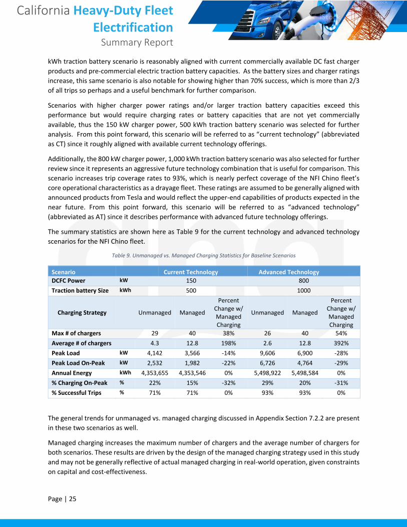
The summary statistics are shown here as Table 9 for the current technology and advanced technology
scenarios for the NFI Chino fleet.
Table 9. Unmanaged vs. Managed Charging Statistics for Baseline Scenarios
Scenario Current Technology Advanced Technology
DCFC Power kW 150 800
Traction battery Size kWh 500 1000
Charging Strategy Unmanaged Managed
Percent Change w/ Managed Charging
Unmanaged Managed
Percent Change w/ Managed Charging
Max # of chargers 29 40 38% 26 40 54%
Average # of chargers 4.3 12.8 198% 2.6 12.8 392%
Peak Load kW 4,142 3,566 -14% 9,606 6,900 -28%
Peak Load On-Peak kW 2,532 1,982 -22% 6,726 4,764 -29%
Annual Energy kWh 4,353,655 4,353,546 0% 5,498,922 5,498,584 0%
% Charging On-Peak % 22% 15% -32% 29% 20% -31%
% Successful Trips % 71% 71% 0% 93% 93% 0%
The general trends for unmanaged vs. managed charging discussed in Appendix Section 7.2.2 are present
in these two scenarios as well.
Managed charging increases the maximum number of chargers and the average number of chargers for
both scenarios. These results are driven by the design of the managed charging strategy used in this study
and may not be generally reflective of actual managed charging in real-world operation, given constraints
on capital and cost-effectiveness.

California Heavy-Duty Fleet Electrification
Summary Report
Page | 26
Managed charging decreases the overall peak load and the on-peak peak load for both scenarios.
Additionally, the percent of charging on-peak is reduced by almost a third in each scenario. These results
are the core goal of managed charging, and together they underscore the importance of charging
management in managing electricity costs and reducing grid impacts.
There is approximately no change in total charging energy, which is expected since the total fleet
operations in terms of vehicle miles traveled (VMT) is the same in both unmanaged and managed
charging.
A comparison of the managed charging baseline CT and AT scenarios is shown as
Table 10 for the NFI Chino fleet. These managed charging baseline scenarios will be used throughout the
remainder of the report.
Table 10. Comparison of Managed Charging for Baseline Scenarios
Scenario
Current Technology
Advanced Technology Difference
DCFC Power kW 150 800 --
Traction battery Size kWh 500 1000 --
Max # of chargers 40 40 0%
Average # of chargers 12.8 12.8 0%
% Successful Trips % 71% 93% 31%
Peak Load kW 3,566 6,900 93%
Peak Load On-Peak kW 1,982 4,764 140%
Annual Energy kWh 4,353,546 5,498,584 26%
% Charging On-Peak % 15% 20% 33%
The AT scenarios represents the highest power charging and largest battery capacity analyzed in this
report. As expected then, the overall peak load and on-peak peak load for the AT scenario are significantly
higher than the CT scenario, with 93% and 140% increases from CT to AT scenarios, respectively.
There is a perhaps non-intuitive result that the overall annual energy consumption is so much higher in
the AT scenario vs. the CT scenario. Upon further inspection, this is a result of the charge-discharge
model including more trips in the CT scenario than the AT scenario. The much larger battery size allows
more successful trips, which in turn results in fewer skipped trips since a skipped trip is required after each
failed trip to reset the charge-discharge algorithm. Including these additional trips results in more overall
energy consumption and is directly related to the higher percentage of successful tripsCalculate Baseline
Costs and Revenues
Following the process outlined at the beginning of Section 4, the next step is to calculate the electricity
costs, infrastructure costs, and LCFS revenues for the baseline scenarios.
5.1.3.1 Baseline Scenario Electricity Costs
Electricity costs are calculated through bill calculations in Table 11 for both managed and unmanaged
charging strategies and for three representative rate types including two Demand Holiday rates (SCE TOU
EV 9) for both Year 1-5 with no demand charge and Year 11 with full demand charge, a Time of Use rate
(SCE TOU 8 D), and Demand Subscription rate (PG&E BEV-2-P).

California Heavy-Duty Fleet Electrification
Summary Report
Page | 27
Table 11. Baseline Scenario Annual Bill Calculations for EV Charging
Scenario Name Rate Name Energy Demand Fixed Total Bill Rate Type
CT Unmanaged SCE TOU EV 9 2 to 50
kV Year 1-5 $636,364 $0 $3,061 $639,424 Demand Holiday
CT Managed SCE TOU EV 9 2 to 50
kV Year 1-5 $578,549 $0 $3,061 $581,609 Demand Holiday
AT Unmanaged SCE TOU EV 9 2 to 50
kV Year 1-5 $894,433 $0 $3,061 $897,493 Demand Holiday
AT Managed SCE TOU EV 9 2 to 50
kV Year 1-5 $789,922 $0 $3,061 $792,983 Demand Holiday
CT Unmanaged SCE TOU EV 9 2 to 50
kV Year 11 $525,505 $437,338 $3,061 $965,904 Demand Holiday
CT Managed SCE TOU EV 9 2 to 50
kV Year 11 $470,269 $400,565 $3,061 $873,895 Demand Holiday
AT Unmanaged SCE TOU EV 9 2 to 50
kV Year 11 $750,901 $973,847 $3,061 $1,727,809 Demand Holiday
AT Managed SCE TOU EV 9 2 to 50
kV Year 11 $651,123 $725,250 $3,061 $1,379,434 Demand Holiday
CT Unmanaged SCE TOU 8 D 2 to 50 kV $350,796 $883,764 $3,061 $1,237,621 TOU
CT Managed SCE TOU 8 D 2 to 50 kV $342,364 $760,266 $3,061 $1,105,691 TOU
AT Unmanaged SCE TOU 8 D 2 to 50 kV $455,963 $2,133,105 $3,061 $2,592,129 TOU
AT Managed SCE TOU 8 D 2 to 50 kV $439,128 $1,595,106 $3,061 $2,037,295 TOU
CT Unmanaged PG&E BEV-2-P $725,817 $70,964 $0 $796,781 Demand
Subscription
CT Managed PG&E BEV-2-P $685,175 $64,997 $0 $750,173 Demand
Subscription
AT Unmanaged PG&E BEV-2-P $997,883 $158,020 $0 $1,155,903 Demand
Subscription
AT Managed PG&E BEV-2-P $929,160 $117,682 $0 $1,046,842 Demand
Subscription
Several conclusions can be drawn from this table.
• Managed charging reduces the bill in all scenarios as compared to unmanaged charging.
• The demand holiday rate SCE EV-9 Year 1-5 shows the lowest bills, and the TOU rate SCE TOU-8-
D shows the highest cost.
• The demand holiday rate SCE EV-9 Year 11, with the demand charge is fully reintroduced, shows
a much higher portion of demand charges comprising the total bill, with nearly 46% of the total
bill for Scenario 2 Managed being demand charges on this rate in Year 11, compared to 0% in Year
1-5.
• The demand subscription rate PG&E BEV-2-P shows modest demand charges and total bills that
are somewhat higher than the SCE EV-9 Year 1 to 5 rate.
5.1.3.2 Baseline Scenario Infrastructure Costs
Estimated infrastructure costs for the NFI baseline scenarios, including installation and the electrical
infrastructure to support them, are described in the following Table 12.

California Heavy-Duty Fleet Electrification
Summary Report
Page | 28
Table 12. Infrastructure cost results
Scenario
Current Technology Managed
Advanced Technology Managed
Advanced Technology Unmanaged
Charger Rating 150 kW 800 kW 800 kW
Illustrative Make/Model ABB Terra 175 HP TBD TBD
Number of Chargers 40 40 26
Peak Power (kW) 6,000 32,000 20,800
EVSE Capital Costs
Power Cabinet + Dispenser $107,000 $375,000 $375,000
Warranty (Increase from 2-5 years) $15,500 $65,250 $65,250
Cable Management $1,500 $1,500 $1,500
Sales Tax (8.5%) $10,540 $37,549 $37,549
Commissioning/Activation Fees $2,000 $2,000 $2,000
Equipment Subtotal $136,540 $481,299 $481,299
EVSE Installation $35,000 $175,000 $175,000
Total Installed Cost (per Charger) $171,540 $656,299 $656,299
Site Work
Utility XFMR and TTM Upgrades Assumed to be covered by utility
Transformers/Switchgears 3 12 8
Switch gear (4000A/480V) $300,000 $1,200,000 $800,000
Secondary Conductors $7,500 $30,000 $20,000
XFMR to Switchgear Connection $37,500 $150,000 $100,000
Circuit Breakers $72,000 $72,000 $46,800
Feeders (assumed 25') $70,000 $70,000 $45,500
Bollards (2 per charger) $64,000 $64,000 $41,600
Total Site Work Cost $551,000 $1,586,000 $1,053,900
Levelized Site Work Cost per Charger $13,775 $39,650 $40,535
Subtotal Scenario Cost $7,412,600 $27,837,950 $18,117,668
Design, Permitting, Management Fees $2,223,780 $8,351,385 $5,435,300
Contingency $741,260 $2,783,795 $1,811,767
Total Scenario Cost $10,377,640 $38,973,130 $25,364,735
EVSE Maintenance ($/year/charger) $3,200 $14,750 $14,750
NPV 20 Year Infrastructure Costs ($10,416,840) ($39,153,818) ($25,545,423)
As described in Section 4.6.2, these infrastructure cost estimates are based on real project estimate data
for similar charger ratings, except for the NFI advanced technology scenario estimates which are scaled
estimates for speculative future products, which contributes some additional uncertainty to these
estimates.
“Total Scenario Costs” is the total capital requirement assumed for year zero in the NPV model. EVSE
maintenance costs (escalated at 3% per year) are included to provide a total 20-year NPV of infrastructure
costs. This NPV is negative since it is a cost, whereas LCFS revenues and DER project revenues NPVs will

California Heavy-Duty Fleet Electrification
Summary Report
Page | 29
be positive. As a reminder, the NPV is method of discounting future costs and/or revenues to make
different project complex economics comparable on an apples-to-apples basis.
The NFI advanced technology scenario requires 40 chargers for managed charging compared to 26
chargers for unmanaged charging, which is a cost difference of about $13 million. For real-world projects,
saving $13 million may justify some scrutiny on the necessity of an additional 14 chargers and if further
optimizations such as charger sharing would make this feasible. This is useful when considering the overall
capital expense on these advanced technology scenarios.
5.1.3.3 Baseline Scenario LCFS Revenues
The electric charging for each baseline scenario qualifies for LCFS credit generation, and the revenues
from selling these LCFS credit on the open market can be a major revenue source for fleet vehicle
electrification projects. Table 13 is showing the annual revenue calculations for three potential charging
pathways, as described in Section 4.6.3.
Table 13. Annual LCFS Revenue Calculations for Baseline Scenarios
EV Carbon Intensity Basis Smart
Charging Grid
Average Renewable/
Zero CI
Current Technology $1,198,583 $1,196,396 $1,495,495
Advanced Technology $1,502,603 $1,511,064 $1,888,829
5.1.4 Apply Optimized DER Project Following the procedure outlined in Section 4.7, the different combinations of PV and energy storage,
including scenarios with PV-only and storage-only, were evaluated using Energy Toolbase. The output
from Energy Toolbase included load profiles of the after-PV and after-PV+Storage performance, using
appropriate settings based on rate (energy-heavy rates get different treatment than demand heavy rates)
and export possibility (PV projects allow for NEM export, and storage-only projects typically do not). The
load profiles were saved for all the modeled DER scenarios.
It should be noted that for the advanced technology scenario, interim results suggested that the original
PV and storage matrix did not consider sufficiently large battery sizes, so several additional battery sizes
were evaluated up to 6 MW / 12 MWh in size.
A rate engine was then applied to the baseline, after-PV, and after-PV-and-Storage load profiles using the
rates required to characterize the project over a 20-year project life. For the SCE TOU-8-D and TOU-8-E
rates (the otherwise applicable commercial rate and the available DER-specific rate), these rates were
assumed fixed as currently published, with a 3% annual rate escalator applied over the 20-year periods.
For the SCE EV-9 rate, which changes over the years 5 to 11 due to the re-introduction of demand charges,
years 1-5, 6, 7, 8, 9, 10, and 11-20 were calculated independently, also with the 3% escalator, which allows
for the complete characterization of the 20-year performance.
Next, the financial model was added to allow calculation of NPV of each DER project scenario.
Next, each PV and Storage size combination was evaluated for rate switch possibility, where it is assumed
the project starts on EV-9, and can change to either TOU-8-D or TOU-8-E in any year if the combined NPV
indicates the rate switch improves the NPV.

California Heavy-Duty Fleet Electrification
Summary Report
Page | 30
Finally, once the rate switch was considered, the best total combined NPV scenario was selected. This
was evaluated for four scenarios for NFI, including for a low PV price and high PV price for both the current
technology and advanced technology baseline scenarios. These summary results are shown in Table 14.
The best DER project overall is the advanced technology, low-price PV scenario with 2500 kW DC PV array
and 5MW / 10MWh energy storage system. This scenario shows a combined positive NPV of $1.7 million
relative to the baseline No-DER project.
The advanced technology low-PV-price scenario has the largest battery of the four scenarios, sized at 5
MW/10 MWh, which represents a $5.5M investment. The rate switch to TOU-8-E occurs immediately in
Year 1, skipping the EV-9 rate for the life of the project. This rate switch result was not expected but is
due to the more favorable TOU-8-E rate characteristics for such large PV and storage DER projects. This
implies the demand holiday EV-9 rate may not be useful for large fleet electrification projects with high
charging power/high battery capacity future technology as well as sufficient space and capital for DER
investments. However, the model assumes that the fleet is electrified to the extent allowed by the charger
and traction battery capacity assumptions in Year 1. This results in high energy throughput in Year 1. Real
fleets are likely to transition the deployment of their fleet to battery-electric vehicles over several years.
Hence, in the early years of the transition, energy throughput will be low, and the EV-9 rate may prove to
be the preferred rate until a sufficient fraction of the fleet is transitioned to battery-electric vehicles.
Out of the two optimal projects for the current technology scenario, the best project is the low PV price
option with 2500 kW DC PV and a 2000 kW / 4000 kWh battery. This battery has a cost of approximately
$2.3 million, substantially less than the advanced technology scenario. This scenario shows a combined
positive NPV of $671,000. The rate switch to TOU-8-E occurs in year 7, which is during the period of
increasing demand charges for the EV-9 rate.
It should be noted that in no scenario was a rate switch to TOU-8-D justified. The higher bill costs on this
rate cannot be sufficiently offset by DER value. PV-only and storage-only scenarios were evaluated, but in
no scenario did they result in better combined NPV than the combined PV and storage scenarios.
Table 14. DER Optimization Results for NFI
Scenario PV Price
DC Power Rating (kW DC)
Power (kW)
Capacity (kWh)
Switch Year
Rate Switch
NPV Charging Costs
NPV DER Project
Combined NPV
CT $2/W 2500 2000 4000 7 TOU 8 E (1,891,499) $2,563,436 $671,936
CT $5/W 1250 1000 4000 9 TOU 8 E (3,696,171) $508,268 ($3,187,903)
AT $2/W 2500 5000 10000 1 TOU 8 E (3,877,778) $5,648,418 $1,770,640
AT $5/W 2500 5000 10000 1 TOU 8 E (3,877,778) $1,689,103 ($2,188,676)
5.1.5 Electrification Project Combined NPV Combining the results of Section 0 and 5.1.4, Table 15 shows the project's combined net present values
layering in the DER project with the LCFS benefits and the electricity and infrastructure costs, to give the
most complete view of project costs. As a reminder, the NPV is method of discounting future costs and/or
revenues to make different project complex economics comparable on an apples-to-apples basis. The
results are presented alongside their respective no-DER baseline scenario for comparison. Note that the
Utility Costs for the DERs project are equal to the no-DERs project because the value of utility bill cost

California Heavy-Duty Fleet Electrification
Summary Report
Page | 31
reductions is reflected in the NPV of the DER Project Cost. The DER Project substantially reduces utility bill
costs, resulting in a net positive NPV for the DER Project Cost line.
Only the current technology scenario is forecasted to result in a positive NPV for the project, with LCFS
revenue and DER project value providing a significant part of the financial value of the project.
Table 15. Combined NPV for baseline grid only versus DER options
Sce
nari
o
PV
Pri
ce
DC
Po
we
r R
ati
ng
(kW
DC
)
Po
we
r (k
W)
Cap
acit
y (
kW
h)
Rate
Sw
itc
h Y
ear
Sta
rt
Rate
Sw
itc
h T
o
NP
V E
lectr
icit
y
Co
st
NP
V D
ER
Pro
ject
NP
V L
CF
S
Rev
en
ue
NP
V
Infr
as
tru
ctu
re
Co
st
NP
V T
ota
l
CT Baseline EV-9, Grid-Only, no DER ($8,969,725) $14,293,294 ($10,416,840) ($5,093,272)
AT Baseline EV-9 Grid-Only, no DER ($13,415,907) $18,052,611 ($39,153,818) ($34,517,114)
CT $2/W 2500 2000 4000 7 TOU 8 E ($8,969,725) $2,563,436 $13,331,803 ($10,416,840) ($3,491,326)
CT $5/W 1250 1000 4000 9 TOU 8 E ($8,969,725) $508,268 $13,812,548 ($10,416,840) ($5,065,749)
AT $2/W 2500 5000 10000 1 TOU 8 E ($13,415,907) $5,648,418 $17,091,120 ($39,153,818) ($29,830,187)
AT $5/W 2500 5000 10000 1 TOU 8 E ($13,415,907) $1,689,103 $17,091,120 ($39,153,818) ($33,789,502)
5.1.6 Other Analysis This section contains other relevant analysis of the modeling results that were not covered by the core
methodology framework outlined in Section 4.2.
5.1.6.1 Load Profile Assessment
The following sample load profiles have been provided for the NFI current technology scenario comparing
the unmanaged versus managed charging algorithms, with 4pm to 9pm on-peak TOU periods highlighted.
To allow for comparison across seasons, a sample week in January and a sample week in July have been
selected. Figure 5 shows the sample load profiles for January for both unmanaged and managed charging
strategy.

California Heavy-Duty Fleet Electrification
Summary Report
Page | 32
Figure 5. Load profile comparison for a week in January for current technology scenario
Evaluation and comparison of unmanaged and managed charging scenarios from the same week
demonstrate that maximum daily peak load can be reduced, on-peak peak load and charging energy can
be reduced, and the base load of the site can be increased from use of a charge management strategy.
These are the expected effects of the managed charging algorithm. Additionally, each day shows both a
primary peak from about 6 AM to 12 PM for unmanaged and 3 to 9AM for managed, and a secondary
peak in the 6 PM-12AM range. This indicates the presence of two-shift operations, common amongst
drayage fleets operating at the Ports of Los Angeles and Long Beach.
The following Figure 6 shows the sample load profiles for July for both unmanaged and managed charging
for the NFI current technology scenario.
Figure 6. Load profile comparison for a week in July for current technology scenario
In this one-week period, a reduction in overall peak load from charge management is present but minimal,
but the reduction in charging peak load and charging energy during the on-peak period is significant, and
the base load has increased. Compared to the January plots which show one clear primary peak from
Tuesday to Friday, July data in the unmanaged scenario shows an early, higher, and almost equivalent
double peak characteristic that may be indicative of higher volume two-shift operation in that season.
5.1.6.2 Impact of DERs on Peak Load
Adding solar PV and energy storage modifies the electric load profile of the charging depot, allowing for
reductions in peak load. Solar PV will sometimes contribute to peak load reduction, although its impact
is variable and hard to predict due to impacts of weather. However, energy storage can be controlled
specifically with goal of “peak shaving” or demand charge management (DCM), which would be the
default on projects using TOU rates or other rates with demand charge components, such as SCE TOU 8
and PG&E E20, or even rates with minor demand charges such as the PG&E BEV-2-P rate or the SCE EV-9
rate once demand charges are reintroduced. The energy storage controls will also seek TOU energy
arbitrage (EA) opportunities to reduce energy costs through NEM, which would apply for all rates including

California Heavy-Duty Fleet Electrification
Summary Report
Page | 33
SCE EV-9. Table 16 shows the peak load reductions that result from optimal DER sizing applied to both
baseline scenarios.
Table 16. Annual Peak Load Reduction from DERs
Scenario ESS Dispatch
Goal Peak Load
(kW) Peak Load
Reduction (kW)
Current Technology DER $2/W EA and DCM 2288 1278
Current Technology DER $5/W EA and DCM 2762 804
Advanced Technology DER EA and DCM 2749 4151
The following Figure 7 shows a sample of three days load profiles for the Current Technology baseline
comparing unmanaged charging, managed charging, and with DER $2/W scenario added. There are three
main energy savings mechanisms that can be distinguished on the load profile plot: (1) peak shaving (2)
TOU energy arbitrage and (3) solar energy savings.
Peak shaving and TOU energy arbitrage are results of the BESS dispatch control and can occur at any time
of day using stored solar energy. Peak shaving can be visually detected by flat horizontal features in the
after-DER curve. TOU energy arbitrage can be visually detected by large negative power exports during
the 4-9pm peak TOU periods.
This contrasts with the solar energy savings as the direct reductions of charging load in mid-day
corresponding to when the sun is shining. Solar energy savings can be visually detected by a significant
reduction in load during the middle of the day, sometimes resulting in export.
Figure 7. Sample Three Days Load Profile DER Comparison
5.1.6.3 Impact of DERs on Electricity Cost
DER modifications to the electric load profile result in electricity cost savings. These savings are the core
part of the investment decision in a DER project since they are the primary driver of return on investment
(ROI). Table 17 shows the Year 1 electricity cost savings after applying the optimized DER project to each
baseline scenario.
Peak Shaving
TOU Energy
Arbitrage
Solar Energy
Savings
Arbitrage

California Heavy-Duty Fleet Electrification
Summary Report
Page | 34
Table 17. Annual Electricity Cost Reduction from DERs20
Scenario Rate Energy
Charges Demand Charges
Fixed Charges Total Bill
Total DER Savings
Current Technology DER $2/W EV-9 $42,521 $0 $3,061 $45,582 $418,631
Current Technology DER $2/W TOU-8-E $42,521 $174,190 $3,061 $219,771 $433,648
Current Technology DER $5/W EV-9 $182,679 $0 $3,061 $185,740 $532,738
Current Technology DER $5/W TOU-8-E $167,902 $239,441 $3,061 $410,404 $624,281
Advanced Technology DER $2/W EV-9 $57,286 $0 $3,061 $60,346 $726,352
Advanced Technology DER $2/W TOU-8-E $57,286 $256,206 $3,061 $316,552 $1,016,746
5.1.6.4 Capital Expenditure and Incentives Analysis
An important consideration outside of the financial value and ROI of a project is the capital required to
undertake a vehicle electrification project in California, which can be offset by incentives such as the
Investment Tax Credit (ITC) and Self Generation Incentive Program (SGIP) and as well as by revenues from
the LCFS program. Table 18 shows a summary of these values. Capital expenditure (Capex) generally
occurs at the beginning of the project, and incentives like ITC also come at the beginning, but SGIP is
staged over five years, and LCFS revenues are ongoing and arrive quarterly.
Most importantly, the capex of the AT scenario is nearly 3 x compared to the two CT scenarios, thus
showing another barrier to making the AT scenario a reality. For the two CT scenarios, even though the
Total Incentive + LCFS NPV is larger than the Capex in both cases, the timing of the SGIP payments and the
long stream of ongoing LCFS payments do not directly affect the need for large capital investments at the
beginning of the project.
Table 18. Capex, Incentives, and LCFS Revenue (In Millions of $)
Scenario Infrastructure
Capex DER Capex Total Capex
ITC + SGIP
Incentive LCFS NPV
Total Incentive + LCFS NPV
Current Technology DER $2/W
$10.4 $7.3 $17.7 $1.8 $13.3 $15.1
Current Technology DER $5/W
$10.4 $8.2 $18.6 $2.4 $13.3 $15.7
Advanced Technology DER
$2/W $39.0 $10.5 $49.5 $3.6 $17.1 $20.7
5.1.6.5 Emissions Reductions
Tailpipe emissions from the baseline diesel fleet are estimated at 6,078 kg NOx and 65.8 kg PM2.5
annually. It is assumed that fleet electrification has the potential to eliminate 100% of these emissions
once full fleet electrification is achieved. However, because this study shows less than 100% successful
trip coverage for all electrification scenarios, the final estimate of emissions reductions is limited by the
fraction of trips successfully electrified.
20 These cost savings figures are based on a Year 1, unescalated savings calculations.

California Heavy-Duty Fleet Electrification
Summary Report
Page | 35
Table 19 summarizes the GHG emissions associated with the baseline fleet and the final electrification
scenarios, under the unmanaged and managed charging strategies, and finally with managed charging
with DERs.
Table 19. Tailpipe carbon dioxide emissions summary (annual emissions from the theoretical fleet transition)
Scenario CT CT AT
PV Price Assumption $2/W PV $5/W PV Both
Total Number of Trucks 50
Annual VMT 2,578,473
Baseline diesel fleet 4782 4782 4782
Electric fleet with unmanaged charging 1377 1377 1870
Electric fleet with managed charging 1289 1289 1684
Electric fleet with managed charging and DERs 304 723 660
All Values metric tons CO2 equivalent
As expected, conversion from diesel to an electric fleet with unmanaged charging achieves significant GHG
reductions. Applying managed charging helps to reduce emissions further. Adding DERs yields additional
emissions reductions, which are proportional to the solar PV size.
5.1.7 Corridor maps The round trip data developed for the NFI Chino fleet was mapped to visualize the primary travel corridors
for the fleet. As shown in Figure 8, the NFI Chino fleet has a broad geographic reach but operates primarily
between the Chino facility and the Ports of Los Angeles and Long Beach. The most traveled roads are the
71, 91, and 710 freeways between Chino and the Ports.
Figure 8. Travel Density Map for NFI Chino Fleet

California Heavy-Duty Fleet Electrification
Summary Report
Page | 36
5.2 Schneider Stockton
5.2.1 Fleet Data Set Summary and Route Characterization Results The provided trip data were parsed into 9515 total round trips for 42 trucks, or 227 average round trips
per truck annually. The trips were 267 miles average, 269 miles median, indicating a normal distribution.
Figure 9 shows a histogram of the round trip distances for the Schneider data set.
By comparison to the NFI data set, the Schneider Stockton fleet has an average trip distance 65% higher
than NFI Chino, and a median trip distance 134% higher than NFI Chino. One contributing factor for this
difference is that Stockton, California is a city within a very rural central valley, meaning everything is more
spread out relative to the urban and suburban characteristics of Southern California.
The corresponding Stockton charging windows are average 22 hours in length, with a median of 13 hours,
showing that very long charging windows of more than 72 hours skew this average higher.21 Figure 10
shows a histogram of the round trip distances for the Schneider data set.
By comparison to the NFI data set, the Schneider Stockton fleet has an average charging window of 110%
longer than NFI Chino, and a median trip charging window of 550% higher than NFI Chino. Given the
charging windows are generally longer and trip distances longer for Schneider Stockton compared to NFI,
we can guess that the Schneider results will be less sensitive to charger rating and more sensitive to
traction battery capacity.
The average percent of round trip mileage on surface streets is 21% versus 79% on highways for the
Schneider fleet.
All results are calculated excluding bad records, as described in Section 4.3.6.
21 Schneider indicated that three of the 42 trucks in the data set do not domicile at the Stockton Intermodal Yard, but rather these trucks stay with their driver who is domiciled elsewhere. This likely explains most of the very long trips before returning to depot. These trips would not be feasible to electrify based on the overnight domicile location but would likely be eliminated in a future electrification scenario where trucks are required to domicile at a fleet facility.

California Heavy-Duty Fleet Electrification
Summary Report
Page | 37
Figure 9. Histogram of Round Trip Distances
Figure 10. Histogram charge window durations for Schneider
5.2.2 Charge-Discharge Model Results
5.2.2.1 Statistics for Unmanaged Charging
The full statistics for unmanaged charging for the sixteen unmanaged charging scenarios are shown in
the Appendix as Table 40 and results for managed charging scenarios are shown in the Appendix as
. The differences for all between managed and unmanaged charging are shown in Appendix Table 42.
Accompanying these full results is Appendix Section 7.2.3 including an analysis of these results to allow
the main body of this report to remain more focused.
5.2.2.2 Failed Trips Characterization
Trips that were not covered successfully are considered “failed”, and it is useful to characterize the failed
trips with some further analysis. First, the large number of “impossible” trips where distance outstrips
the battery capacity in many scenarios is the most significant factor for the Schneider fleet, as discussed
above in Section 5.2.2.1. For example, in the scenario with 150 kW charger rating and 1000 kWh battery
capacity, there are only 57 trips that were both possible and failed, which is quite small compared to the
total number of 9,475 trips, a ratio of 0.6%; this compares to the NFI result for the same scenario where
the possible and failed trips ratio was much higher at 14.3%. This indicates for the Schneider fleet that
there is little room for improvement from slight operational changes such as increasing the time at the
depot for charging.
The following Figure 11 characterizes these 57 failed trips for the selected baseline scenario, and shows
that most failed trips need 30 minutes or less of additional charging time to be successfully completed.

California Heavy-Duty Fleet Electrification
Summary Report
Page | 38
Figure 11. Minutes of additional charge window needed to make failed trip successful for the 150 kW charger power and 1000 kWh battery capacity scenario
Several observations are drawn from the comparison of managed charging with unmanaged charging.
Similar to NFI, managed charging requires both more installed chargers (between 6% and 100% increase)
and increases the average number of chargers utilized (between 6% and 308% increase) as compared to
unmanaged charging. Again, this is largely a result of the assumption that there is no limit in the model
for the maximum number of chargers together with the fact that managed charging strategy was defined
to reducing the charge power to the minimum required to charge the truck over the available charging
window. For scenarios with very high-power chargers, this approach results in the chargers typically
operating at only a small fraction of their power rating. Because the current analysis does not model the
“charger sharing” approach of rotating trucks through a single charging stall (similar to a diesel fueling
station operation), the required number of chargers for scenarios with high-power chargers (350 kW and
800 kW) is likely overstated.
Second, and also similar to NFI, managed charging reduces peak load (both on-peak and all day) as well
as the energy consumption during on-peak periods. This result was expected since the charging algorithm
was designed to achieve this type of result. Noteworthy are the scenarios where managed charging almost
eliminates on-peak charging with reductions up to 92%. The largest reduction in on-peak peak load was
69% for the scenario with 350 kW charger power and 500 kWh traction battery rating, corresponding to
a drop of 1.28 MW when using managed charging. These results speak to the high potential impact for
managed charging in mitigating grid impacts and electricity costs.
Also similar to NFI, the scenarios with high-power chargers (350 kW and 800 kW) show a greater percent
reduction in peak load and on-peak peak load compared to the lower-power chargers, which indicates the
greater potential for impact of managed charging strategy when using high-power chargers. Also, the
percent reduction in on-peak energy consumption remains more uniform across the scenarios.
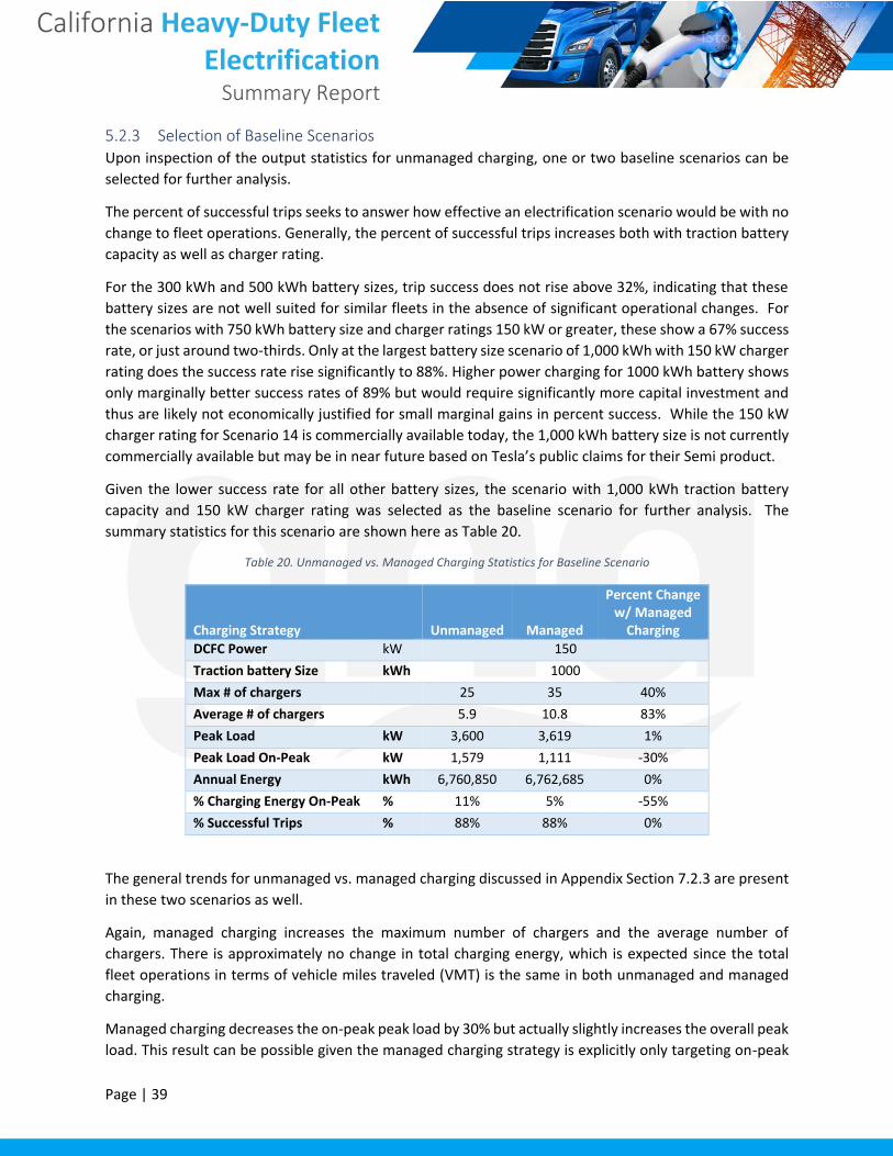
California Heavy-Duty Fleet Electrification
Summary Report
Page | 39
5.2.3 Selection of Baseline Scenarios Upon inspection of the output statistics for unmanaged charging, one or two baseline scenarios can be
selected for further analysis.
The percent of successful trips seeks to answer how effective an electrification scenario would be with no
change to fleet operations. Generally, the percent of successful trips increases both with traction battery
capacity as well as charger rating.
For the 300 kWh and 500 kWh battery sizes, trip success does not rise above 32%, indicating that these
battery sizes are not well suited for similar fleets in the absence of significant operational changes. For
the scenarios with 750 kWh battery size and charger ratings 150 kW or greater, these show a 67% success
rate, or just around two-thirds. Only at the largest battery size scenario of 1,000 kWh with 150 kW charger
rating does the success rate rise significantly to 88%. Higher power charging for 1000 kWh battery shows
only marginally better success rates of 89% but would require significantly more capital investment and
thus are likely not economically justified for small marginal gains in percent success. While the 150 kW
charger rating for Scenario 14 is commercially available today, the 1,000 kWh battery size is not currently
commercially available but may be in near future based on Tesla’s public claims for their Semi product.
Given the lower success rate for all other battery sizes, the scenario with 1,000 kWh traction battery
capacity and 150 kW charger rating was selected as the baseline scenario for further analysis. The
summary statistics for this scenario are shown here as Table 20.
Table 20. Unmanaged vs. Managed Charging Statistics for Baseline Scenario
Charging Strategy Unmanaged Managed
Percent Change w/ Managed
Charging
DCFC Power kW 150
Traction battery Size kWh 1000
Max # of chargers 25 35 40%
Average # of chargers 5.9 10.8 83%
Peak Load kW 3,600 3,619 1%
Peak Load On-Peak kW 1,579 1,111 -30%
Annual Energy kWh 6,760,850 6,762,685 0%
% Charging Energy On-Peak % 11% 5% -55%
% Successful Trips % 88% 88% 0%
The general trends for unmanaged vs. managed charging discussed in Appendix Section 7.2.3 are present
in these two scenarios as well.
Again, managed charging increases the maximum number of chargers and the average number of
chargers. There is approximately no change in total charging energy, which is expected since the total
fleet operations in terms of vehicle miles traveled (VMT) is the same in both unmanaged and managed
charging.
Managed charging decreases the on-peak peak load by 30% but actually slightly increases the overall peak
load. This result can be possible given the managed charging strategy is explicitly only targeting on-peak

California Heavy-Duty Fleet Electrification
Summary Report
Page | 40
peak load as the goal. Additionally, the percent of charging on-peak is reduced by 55%, representing a
significant reduction. These results are the core goal of managed charging, and together they underscore
the importance of charging management in managing electricity costs and reducing grid impacts.
5.2.4 Calculate Baseline Costs and Revenues Following the process outlined at the beginning of Section 4, the next step is to calculate the electricity
costs, infrastructure costs, and LCFS revenues for the baseline scenarios.
5.2.4.1 Baseline Scenario Electricity Costs
Bill calculations for the Schneider core charging-only results are given in Table 21.
for both managed and unmanaged and for three representative rate types including a Demand
Subscription rate (PG&E BEV-2-P), a Time of Use (TOU) rate (PG&E B-20), and two Demand Holiday rates
(SCE TOU EV 9) for both Year 1-5 with no demand charge and for Year 11 with full demand charge.
Table 21. Baseline Annual Bill Calculations for EV Charging
Charging Strategy Rate Name Energy Demand Fixed Total Bill Rate Type
Unmanaged PG&E BEV-2-P $912,566 $69,277 $0 $981,843 Demand Subscription
Managed PG&E BEV-2-P $896,881 $63,125 $0 $960,006 Demand Subscription
Unmanaged PG&E B-20 Primary $719,299 $977,482 $542 $1,697,323 TOU
Managed PG&E B-20 Primary $701,562 $874,834 $542 $1,576,937 TOU
Unmanaged SCE TOU EV 9 2 to 50 kV Year 1-5 $797,129 $0 $3,061 $800,190 Demand Holiday
Managed SCE TOU EV 9 2 to 50 kV Year 1-5 $711,439 $0 $3,061 $714,499 Demand Holiday
Unmanaged SCE TOU EV 9 2 to 50 kV Year 11 $633,773 $426,938 $3,061 $1,063,772 Demand Holiday
Managed SCE TOU EV 9 2 to 50 kV Year 11 $552,590 $389,024 $3,061 $944,675 Demand Holiday
Several conclusions can be drawn from this table.
• The managed charging clearly reduces the bill in all scenarios compared to unmanaged charging.
• Southern California Edison (SCE) EV-9 rate with a demand charge holiday during Year 1-5 shows
the lowest bills, and the PG&E TOU rate B-20 rate shows the highest.
• The demand subscription PG&E rate shows modest demand charges and total bills that are higher
than the SCE EV-9 Year 1 to 5 rate but reaching a similar value on the Year 11 version of SCE EV-
9.

California Heavy-Duty Fleet Electrification
Summary Report
Page | 41
5.2.4.2 Baseline Scenario Infrastructure Costs
Estimated infrastructure costs for Schneider, including installation and the electrical infrastructure to
support them, are described in Table 22.
Table 22. Infrastructure costs results
Category Value
Charger Rating 150 kW
Illustrative Make/Model ABB Terra 175 HP
Number of Chargers 35
Peak Power (kW) 5250
EVSE
Power Cabinet + Dispenser $107,000
Warranty (Increase from 2-5 years) $15,500
Cable Management $1,500
Sales Tax (8.5%) $10,540
Commissioning/Activation Fees $2,000
Equipment Subtotal $136,540
EVSE Installation $35,000
Total Installed Cost (per Charger) $171,540
Site Work
Utility XFMR and TTM Upgrades Assumed by utility
Transformers/Switchgears 2
Switch gear (4000A/480V) $200,000
Secondary Conductors $5,000
XFMR to Switchgear Connection $25,000
Circuit Breakers $63,000
Feeders (assumed 25') $61,250
Bollards (2 per charger) $56,000
Total Site Work Cost $410,250
Levelized Site Work Cost per Charger $11,721
Subtotal Scenario Cost $6,414,150
Design, Permitting, Management Fees
$1,924,245
Contingency $641,415
Total Scenario Cost $8,979,810
EVSE Maintenance ($/year/charger) $3,200
NPV 20 Year Infrastructure Costs ($9,019,010)
As described in Section 4.6.2, these estimates are based on recent project experience for similarly sized
chargers. “Total Scenario Costs” is the total capital requirement assumed for year zero in the NPV model.
EVSE maintenance costs (escalated at 3% per year) are included to provide a total 20-year NPV of
infrastructure costs. This NPV is negative since it is a cost, whereas LCFS revenues and DER project
revenues NPVs will be positive. As a reminder, the NPV is method of discounting future costs and/or
revenues to make different project complex economics comparable on an apples-to-apples basis.

California Heavy-Duty Fleet Electrification
Summary Report
Page | 42
5.2.4.3 Baseline Scenario LCFS Revenues
The electric charging for each baseline scenario qualifies for LCFS credit generation, and the revenues
from selling these LCFS credit on the open market can be a major revenue source for fleet vehicle
electrification projects. Table 23 is showing the annual revenue calculations for three potential charging
pathways, as described in Section 4.6.3.
Table 23. Annual LCFS Revenue Calculations for Baseline Scenarios
EV Carbon Intensity Basis Smart
Charging Grid Average Renewable/
Zero CI
LCFS Revenue $1,922,126 $1,858,451 $2,323,063
5.2.5 Apply Optimized DER Project Following the procedure outline in Section 4.7, the different combinations of PV and energy storage,
including scenarios with PV-only and storage-only, were evaluated using Energy Toolbase. The output
from Energy Toolbase included load profiles of the after-PV and after-PV+Storage performance, using
appropriate settings based on rate (energy-heavy rates get different treatment than demand heavy rates)
and export possibility (PV projects allow for NEM export, and storage-only projects typically do not). The
load profiles were saved for all the modeled DER scenarios.
A rate engine was then applied to the baseline, after-PV, and after-PV-and-Storage load profiles using the
rates required to characterize the project over a 20-year project life. Since Schneider is in PG&E’s service
territory, the baseline rate was BEV-2-P, with additional calculations for rates PG&E rates B-20 Primary
and B-20 R Primary (the otherwise applicable commercial rate, and the available DER-specific rate). These
rates were assumed fixed as currently published, with a 3% annual rate escalator applied over the 20-year
periods.
Next, the financial model was added to allow the calculation of NPV of each DER project scenario.
Next, each PV and Storage size combination was evaluated for rate switch possibility, where it is assumed
the project starts on BEV-2-P, and can change to either B-20 or to B-20 R in any year if the combined NPV
indicates the rate switch improves the NPV.
Finally, once the rate switch was considered, the best total combined NPV scenario was selected. This
was evaluated for two scenarios for Schneider, including for a low PV price and high PV price. The
summary results are shown in Table 24.
The low PV price scenario of $2/W has a positive DER project result, with this scenario showing a combined
positive NPV of $2.6 million relative to the baseline No-DER project.
Note that the rate switch is not favorable for any year over the life of the project, hence the baseline rate
of BEV-2-P continues to apply for all 20 years. This implies the demand subscription BEV-2-P rate is the
best currently available rate for large fleet electrification projects with currently available charger ratings,
and for future high EV battery capacity ratings when combined with sufficient space and capital for DER
investments.

California Heavy-Duty Fleet Electrification
Summary Report
Page | 43
The high PV price scenarios resulted only in negative NPV projects, so this is excluded from further
analysis. It should be noted that for the high PV price scenario of $5/W, no DER project resulted in a
positive combined NPV, even considering PV only and storage only options.
Table 24. DER optimization results for Schneider
Scenario PV Price
DC Power Rating
(kW DC) Power (kW)
Capacity (kWh)
NPV Charging
Costs NPV DER Project
Combined NPV
w/ DER $2/W 3600 2500 5000 ($1,509,761) $4,113,692 $2,603,930
5.2.6 Electrification Project Combined NPV Combining the results of Section 5.2.4 and 5.2.5,
Table 25 shows the project's combined net present values layering in the DER project with the LCFS
benefits and the electricity and infrastructure costs, to give a more complete view of project costs. As a
reminder, the NPV is method of discounting future costs and/or revenues to make different project
complex economics comparable on an apples-to-apples basis. The results are presented alongside their
respective no-DER baseline scenario for comparison. The electrification project is forecasted to result in
a positive NPV for the project, with LCFS revenue and DER project value providing a significant part of the
financial value of the project.
Table 25. Combined NPV for baseline grid only versus DER options
Sce
nar
io
PV
Pri
ce
DC
Po
we
r R
atin
g
(kW
DC
)
Po
we
r (k
W)
Cap
acit
y (k
Wh
)
NP
V C
har
gin
g
Co
sts
NP
V D
ER P
roje
ct
NP
V L
CFS
Re
ven
ue
NP
V
Infr
astr
uct
ure
Co
st
NP
V T
ota
l
Baseline Baseline BEV-2-P, Grid-Only, no DER ($11,760,115)
$22,202,830 ($9,019,010) $1,423,705
w/ DER $2/W 3600 2500 5000
($1,509,761) $4,113,692 $20,814,259 ($9,019,010) $14,399,179
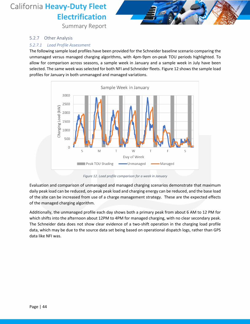
California Heavy-Duty Fleet Electrification
Summary Report
Page | 44
5.2.7 Other Analysis
5.2.7.1 Load Profile Assessment
The following sample load profiles have been provided for the Schneider baseline scenario comparing the
unmanaged versus managed charging algorithms, with 4pm-9pm on-peak TOU periods highlighted. To
allow for comparison across seasons, a sample week in January and a sample week in July have been
selected. The same week was selected for both NFI and Schneider fleets. Figure 12 shows the sample load
profiles for January in both unmanaged and managed variations.
Figure 12. Load profile comparison for a week in January
Evaluation and comparison of unmanaged and managed charging scenarios demonstrate that maximum
daily peak load can be reduced, on-peak peak load and charging energy can be reduced, and the base load
of the site can be increased from use of a charge management strategy. These are the expected effects
of the managed charging algorithm.
Additionally, the unmanaged profile each day shows both a primary peak from about 6 AM to 12 PM for
which shifts into the afternoon about 12PM to 4PM for managed charging, with no clear secondary peak.
The Schneider data does not show clear evidence of a two-shift operation in the charging load profile
data, which may be due to the source data set being based on operational dispatch logs, rather than GPS
data like NFI was.

California Heavy-Duty Fleet Electrification
Summary Report
Page | 45
The following Figure 13 shows the sample load profiles for July for both unmanaged and managed
charging.
Figure 13. Load profile comparison for a week in July
Again, the late morning to mid-day peak is shown here, but the operations appear to be shifted by one to
two days, with the peaks running from Saturday to Wednesday. Peak loads are only slightly reduced,
except for a clear reduction on Tuesday. However, on-peak peak loads and on-peak charging energy are
reduced by managed charging, especially on Sunday.
5.2.7.2 Impact of DERs on Peak Load
Adding solar PV and energy storage modifies the electric load profile of the charging depot, allowing for
reductions in peak load. Solar PV will sometimes contribute to peak load reduction, although its impact
is variable and hard to predict due to the impacts of weather. However, energy storage can be controlled
specifically with the goal of “peak shaving” or demand charge management (DCM), which would be the
default on projects using TOU rates or other rates with demand charge components, such as SCE TOU 8
and PG&E E20, or even rates with minor demand charges such as the PG&E BEV-2-P rate or the SCE EV-9
rate once demand charges are reintroduced. The energy storage controls will also seek TOU energy
arbitrage (EA) opportunities to reduce energy costs through NEM, which would apply for all rates including
SCE EV-9.
Table 26 shows the peak load reductions that result from optimal DER sizing applied to both baseline
scenarios.
Table 26. Annual Peak Load Reduction from DERs
Scenario ESS Dispatch
Goal Peak Load
(kW) Peak Load
Reduction (kW)
Baseline w DER EA and DCM 3008 611
The following Figure 14 shows a sample of three days load profiles for the baseline scenario comparing
unmanaged charging, managed charging, and with DER added. There are three main energy savings

California Heavy-Duty Fleet Electrification
Summary Report
Page | 46
mechanisms that can be distinguished on the load profile plot: (1) peak shaving (2) TOU energy arbitrage
and (3) solar energy savings.
Peak shaving and TOU energy arbitrage are results of the BESS dispatch control and can occur at any
time of day using stored solar energy. Peak shaving can be visually detected by flat horizontal features
in the after-DER curve, although this can sometimes occur due to co-incident solar generation and result
in non-flat features. TOU energy arbitrage can be visually detected by energy reductions during the 4-
9pm peak TOU periods, but this activity is less present for the Schneider results than for NFI.
This contrasts with the solar energy savings as the direct reductions of charging load in mid-day
corresponding to when the sun is shining. Solar energy savings can be visually detected by a significant
reduction in load during the middle of the day, sometimes resulting in export. This characteristic is very
significant here due to the large loads from managed charging that occur during the middle of the day.
Figure 14. Sample Three Days Load Profile DER Comparison
Peak Shaving TOU Energy
Arbitrage
Solar Energy Savings

California Heavy-Duty Fleet Electrification
Summary Report
Page | 47
5.2.7.3 Impact of DERs on Electricity Cost
DER modifications to the electric load profile result in electricity cost savings. These savings are the core
part of the investment decision in a DER project since they are the primary driver of return on investment
(ROI). Table 27 shows the electricity cost savings after applying the optimized DER project to each
scenario.
Table 27. Annual Electricity Cost Reduction from DERs22
Scenario Rate Energy
Charges Demand Charges
Fixed Charges Total Bill
Total DER Savings
Baseline with DER BEV-2-P $78,087 $45,158 $0 $123,245 $836,761
5.2.7.4 Capital Expenditure and Incentives Analysis
An important consideration outside of the financial value and ROI of a project is the capital required to
undertake a vehicle electrification project in California, which can be offset by incentives such as the
Investment Tax Credit (ITC) and Self Generation Incentive Program (SGIP) and as well as by revenues from
the LCFS program. Table 28 shows a summary of these values.
Again, even though the Total Incentive + LCFS NPV is actually larger than the Total Capex, the timing of
the SGIP payments and the long stream of ongoing LCFS payments do not directly affect the need for large
capital investments at the beginning of the project.
Table 28. Capex, Incentives, and LCFS Revenue (In Millions of $)
Scenario Infrastructure
Capex DER Capex Total Capex
ITC + SGIP
Incentive LCFS NPV
Total Incentive + LCFS NPV
Baseline with DER $9.0 $10.0 $19.0 $3.4 $22.2 $25.6
5.2.7.5 Emissions Reductions
Tailpipe emissions from the baseline diesel fleet are estimated at 6,240 kg NOx and 69 kg PM2.5 annually.
It is assumed that fleet electrification has the potential to eliminate 100% of these emissions once full
fleet electrification is achieved. However, because this study shows less than 100% successful trip
coverage for all electrification scenarios, the final estimate of emissions reductions is limited by the
fraction of trips successfully electrified.
Table 29 summarizes the GHG emissions associated with the baseline fleet and the final electrification
scenarios, under the unmanaged and managed charging strategies, and finally with managed charging
with DERs.
Like the NFI scenario, conversion from diesel to an electric fleet with unmanaged charging achieves
significant GHG reductions. Applying managed charging helps to reduce emissions further. Adding DERs
yields additional emissions reductions, proportional to the solar PV size.
Table 29. Carbon dioxide emissions reductions summary for Schneider
22 These cost savings figures are based on a Year 1, unescalated savings calculations.

California Heavy-Duty Fleet Electrification
Summary Report
Page | 48
Scenario Baseline
Number of Trucks 42
Annual VMT 2,821,738
Baseline diesel fleet (MT CO2e/year) 5295
Electric fleet with unmanaged charging (MT CO2e/year) 1831
Electric fleet with managed charging (MT CO2e/year) 1700
Electric fleet with managed charging and DERs (MT CO2e/year) 320
5.2.8 Corridor maps The round trip data developed for the Schneider Stockton fleet was mapped to visualize the primary travel
corridors for the fleet. As shown in Figure 8, the Schneider Stockton fleet has a broad geographic reach.
The most significant corridor is along Highway 99 between Stockton and Fresno, but operations are less
concentrated on this corridor as a fraction of total trips than the concentrations seen in the NFI Chino
fleet trips to the Ports of Los Angeles and Long Beach. This is most likely because the Schneider fleet
facility is located adjacent to the BNSF Stockton railyard, a primary origin/destination for trips operating
out of the Schneider facility.
Figure 15. Travel Density Map for Schneider Stockton Fleet

California Heavy-Duty Fleet Electrification
Summary Report
Page | 49
5.3 Results Summary and Comparison This section summarized and compares the results for the Schneider and NFI fleets.
These fleets are similar in several ways. Both fleets are regional goods movement fleets operating Class 8
semi-tractors in California. Additionally, they operate primarily on a return-to-base basis and serve a major
intermodal cargo facility. However, the details of their operations drive substantially different results with
respect to traction battery capacities and recommendations for DER sizing. These differences also result
in significantly different average costs of delivered energy for EV charging.
Baseline scenarios of traction battery capacity and charging power were selected, with two scenarios for
the NFI fleet and one for the Schneider fleet, based on the fraction of trips that could be electrified and
anticipated costs for each combination. These baseline scenarios were selected from a cost analysis of 16
combinations of traction battery capacity and charging rate for each fleet, under two charge management
strategies. Table 30 summarizes key statistics of the three baseline scenarios.
Table 30. Summary of Managed Charging Baseline Scenarios
Fleet Schneider NFI NFI Scenario Baseline Current Technology Advanced Technology
DCFC Power Level (kW) 150 150 800
Traction battery Capacity (kWh) 1,000 500 1,000
% of Successful Trips 88% 71% 93%
Annual Charging Energy (kWh) 6,762,685 4,353,546 5,498,584
Peak Load (kW) 3,619 3,566 6,902
Reduction in Peak Load (kW) -19 576 2,704
On-Peak Load (kW) 1,111 1,982 4,764
Reduction in Peak Load On-Peak (kW) 468 693 2,475
Reduction in Charging On-Peak (%) -55% -32% -31%
Maximum Number of Chargers in Use 35 40 40
% of Successful Trips 88% 71% 93%
5.3.1 Impact of Distributed Energy Resources A DER sizing and optimization analysis was then performed for each of the three scenarios and the
configurations producing the lowest cost on a 20-year Net Present Value (NPV) basis were identified.
Rate switching was evaluated to determine if other rates besides the special EV rates would help the
project economics. The results of the DER sizing optimization are shown in Table 31.

California Heavy-Duty Fleet Electrification
Summary Report
Page | 50
Table 31. Optimized DER Sizing for Baseline Scenarios
Fleet Schneider NFI NFI
Scenario Baseline CT AT
Assumed Installed PV Cost ($/kW) $2.00 $2.00 $2.00
PV Array Size (kW DC) 3,600 2,500 2,500
Energy Storage System (ESS) Power (kW) 2,500 2,000 5,000
ESS Capacity (kWh) 5,000 4,000 10,000
NPV DER Project $4,113,692 $2,563,436 $5,648,418
Reduction in Peak Load (kW) 611 1,278 4,151
Rate Switch Stay on PG&E BEV-2-P Switch in Year 7 to SCE TOU-8-E
Switch Immediately to SCE TOU-8-E
5.3.2 Conclusions on 20 Year Combined Economics The results of the cost analysis are shown in Table 32 and Figure 16. The results shown in Table 32 compare
the 20-year NPV of utility costs, DER Project Costs, LCFS Revenues, and Charging Infrastructure costs for
each selected scenario, with and without the implementation of DERs. Note that the Utility Costs for the
DERs project are equal to the no-DERs project because the value of utility bill cost reductions is reflected
in the NPV of the DER Project Cost. The DER Project substantially reduces utility bill costs, resulting in a
net positive NPV for the DER Project Cost line.
The Schneider scenario shows a positive total NPV, which must be considered in the context that it
includes a traction battery of 1000 kWh that does not exist commercially as this report was published in
2020. The NFI current technology scenario shows a moderate negative NPV using commercially available
technology, which relies heavily on the LCFS contribution with a smaller contribution from DERs. The NFI
advanced technology scenario shows a large negative NPV, which is driven by the extreme EVSE
infrastructure costs from a larger number of very high power chargers and supporting infrastructure. This
future 800 kW charger does not exist commercially, and there is surely uncertainly in the infrastructure
cost estimate, but this result underscores the difficultly today with considering these advanced EV
technologies.
Table 32. 20-Year Total NPV Comparison
Fleet Schneider NFI NFI Scenario Baseline Current Technology Advanced Technology
DER Used Yes No Yes No Yes No
NPV Electricity
($11,760,115) ($11,760,115) ($8,969,725) ($8,969,725) ($13,415,907) ($13,415,907)
NPV DER $4,113,692 $0 $2,563,436 $0 $5,648,418 $0
NPV LCFS Revenue
$20,814,259 $22,202,830 $13,331,803 $14,293,294 $17,091,120 $18,052,611
NPV EVSE Infrastructure
($9,019,010) ($9,019,010) ($10,416,840) ($10,416,840) ($39,153,818) ($39,153,818)
20-Year Total NPV
$4,148,826 $1,423,705 ($3,491,326) ($5,093,271) ($29,830,187) ($34,517,114)

California Heavy-Duty Fleet Electrification
Summary Report
Page | 51
In the following Table 33, the baseline electricity costs NPV ranges from -$0.087 to -$0.122 per kWh
delivered to the EV (net of charging efficiency losses) for each scenario. Implementation of DER improves
the NPV of delivered energy ranging from $0.029 to $0.051 per kWh. LCFS revenues are the most
significant contributor of positive NPV with a range of $0.153 to $0.164 cents per kWh. EVSE infrastructure
cost NPV varies widely, with the Schneider fleet estimated at -$0.067 per kWh, and the NFI fleet estimated
at -$0.12 to -$0.356 per kWh. Schneider’s lower infrastructure cost NPV per kWh are a result of fewer
chargers required (25 vs 40) and higher annual energy throughput relative to the NFI scenarios. NFI’s
infrastructure costs for the AT scenario are very high owing to the large number of chargers and the very
high-power levels assumed. Given these high costs and limitations of the charge management model
discussed later in this section, it is unlikely that a fleet would pursue a solution like the AT scenario, despite
the scenario maximizing the percentage of trips successfully electrified.
Table 33. 20-Year NPV Per Delivered kWh Energy
Fleet Schneider NFI NFI Scenario Baseline Current Technology Advanced Technology
DER Used Yes No Yes No Yes No
Annual Delivered Energy (kWh)
6,760,850 6,760,850 4,353,541 4,353,541 5,498,604 5,498,604
20-year NPV Per Delivered kWh ($/kWh)
$0.031 $0.011 ($0.040) ($0.058) ($0.271) ($0.314)
NPV Electricity ($0.087) ($0.087) ($0.103) ($0.103) ($0.122) ($0.122)
NPV DER $0.030 $0.000 $0.029 $0.000 $0.051 $0.000
NPV LCFS Revenue $0.154 $0.164 $0.153 $0.164 $0.155 $0.164
NPV EVSE Infrastructure
($0.067) ($0.067) ($0.120) ($0.120) ($0.356) ($0.356)
Figure 16 summarizes the net present value buildup per charging kWh for each scenario with DER
implemented. As shown, the NPV per delivered kWh to Schneider on a 20-year NPV basis is approximately
+$0.03 cents per kWh, meaning that LCFS revenues and DER benefits more than offset the cost of
electricity and charging infrastructure. For the NFI current technology scenario, the NPV per delivered
kWh is -$0.04 per kWh, owning to higher infrastructure and electricity costs that are not fully offset by
LCFS revenues and DER benefits.
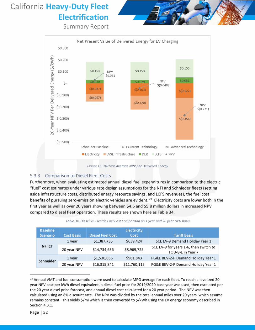
California Heavy-Duty Fleet Electrification
Summary Report
Page | 52
Figure 16. 20-Year Average NPV per Delivered Energy
5.3.3 Comparison to Diesel Fleet Costs Furthermore, when evaluating estimated annual diesel fuel expenditures in comparison to the electric
“fuel” cost estimates under various rate design assumptions for the NFI and Schnieder fleets (setting
aside infrastructure costs, distributed energy resource savings, and LCFS revenues), the fuel cost
benefits of pursuing zero-emission electric vehicles are evident. 23 Electricity costs are lower both in the
first year as well as over 20 years showing between $4.6 and $5.8 million dollars in increased NPV
compared to diesel fleet operation. These results are shown here as Table 34.
Table 34. Diesel vs. Electric Fuel Cost Comparison on 1 year and 20 year NPV basis
Baseline Scenario Cost Basis Diesel Fuel Cost
Electricity Cost Tariff Basis
NFI CT 1 year $1,387,735 $639,424 SCE EV-9 Demand Holiday Year 1
20 year NPV $14,734,636 $8,969,725 SCE EV-9 for years 1-6, then switch to
TOU-8-E in Year 7
Schneider 1 year $1,536,656 $981,843 PG&E BEV-2-P Demand Holiday Year 1
20 year NPV $16,315,841 $11,760,115 PG&E BEV-2-P Demand Holiday Year 1
23 Annual VMT and fuel consumption were used to calculate MPG average for each fleet. To reach a levelized 20 year NPV cost per kWh diesel equivalent, a diesel fuel price for 2019/2020 base year was used, then escalated per the 20 year diesel price forecast, and annual diesel cost calculated for a 20 year period. The NPV was then calculated using an 8% discount rate. The NPV was divided by the total annual miles over 20 years, which assume remains constant. This yields $/mi which is then converted to $/kWh using the EV energy economy described in Section 4.3.1.

California Heavy-Duty Fleet Electrification
Summary Report
Page | 53
The final NPV breakdown shown above for the Schneider and NFI CT scenarios are supportive of
electrification when compared to diesel fuel costs on an equivalent basis as shown below in Table 35.23
By calculating a diesel NPV over 20 years and converting to an equivalent $/kWh, a baseline electrification
case for both fleets is calculated and results in net savings in terms of positive NPV difference of
$0.15/kWh and $0.02/kWh respectively for Schneider and NFI. This means that net of real infrastructure
and electricity costs estimates, as well as support from LCFS and DER revenues, electrification can provide
real value over diesel in terms of fuel cost today.
Table 35. Comparison of Diesel vs Electric fuel costs on per kWh basis
Scenario 20-yr NPV per Mile Diesel24,25
EV Energy Economy (kWh/mi)
20-yr NPV per kWh Diesel equivalent
20-yr NPV per Delivered kWh
Positive NPV Difference per kWh
Schneider ($0.289) 2.4 ($0.120) $0.031 $0.151
NFI CT ($0.289) 2.1 ($0.057) ($0.040) $0.013
However, this also highlights the dependence of heavy-duty electric transportation economics on LCFS
revenues. Absent LCFS revenues of about $0.15/kWh from Table 33, the positive results compared to
diesel are erased. In the absence of LCFS revenues, this leaves no cost reduction to offset the higher capital
costs of the electric trucks themselves. Improvements in infrastructure cost and electricity costs through
charging management or improvements in DER project value would need to make up for this potential
loss in LCFS revenue.
5.3.4 Conclusions on Capital Expenditure and Financing Table 36 shows a summary of the capital expenditures for the charging infrastructure and DER project.
This is included to help underscore the significant capital requirements for EVSE infrastructure as well as
DER projects, which of course are in addition to the capital requirements for the electric trucks themselves
which are not considered in this study. These large capital requirements make fleet electrification
decisions more feasible for companies with large balance sheets and sufficient cash reserves, otherwise,
financing mechanisms will need to be considered, which contribute to increased costs to access the
required capital. Additionally, while DER provides a net cost reduction on a 20-year basis, the DER projects
substantially more capital intensive, requiring up to twice the capital expenditures in Year 0 compared to
their non-DER alternatives. A 20-year payback is typical of utility and industrial-scale energy projects but
is an uncommonly long analysis period for most truck fleets, which is typically 10 years or less. Hence,
mechanisms to move capital expenditures to entities with appetites for 20-year returns may increase the
willingness of fleets to invest in DER projects.
Also provided are the total incentives and the NPV of LCFS revenues over the 20-year period for
comparison to the capital expenditures. This shows the significance of public policy support for fleet
electrification projects.
24 Baseline diesel price estimated for base year 2019/2020 and escalated over 20 years. US EIA, Weekly Retail Gasoline and Diesel Prices. https://www.eia.gov/dnav/pet/pet_pri_gnd_dcus_sca_a.htm 25 US EIA, Annual Energy Outlook 2020, Data A3. https://www.eia.gov/outlooks/aeo/

California Heavy-Duty Fleet Electrification
Summary Report
Page | 54
Table 36. CapEx Summary (In Millions of $)
Fleet Schneider NFI NFI Scenario Baseline Current Technology Advanced Technology
DER Used Yes No Yes No Yes No
Year 0 Capex (DER)
($10.9) $0 ($7.3) $0 ($10.5) $0
Year 0 Capex (Infrastructure)
($9.0) ($9.0) ($10.4) ($10.4) ($39.0) ($39.0)
Year 0 Total Capex
($19.8) ($9.0) ($17.7) ($10.4) ($49.5) ($39.0)
ITC + SGIP Incentive
$3.4 $0 $1.8 $0 $3.6 $0
LCFS NPV $20.8 $22.2 $13.3 $14.3 $17.1 $18.1
Total Incentive + LCSF NPV
$23.2 $22.2 $15.1 $14.3 $20.7 $18.1
6 Conclusions for Fleets and Utilities The analysis of the NFI Chino and Schneider Stockton fleets indicates that current or near-term EV
technologies can support 70 to 88 percent of local goods movement trips without significant operational
changes at these facilities. Some operational adjustments to increase charging windows by 30 to 70
minutes, or through the use of offsite en-route charging, could significantly increase the number of trips
that may be electrified if these operational adjustments are not significantly disruptive to the fleet.
Very high-power charging (350 kW and greater) does not appear to be necessary to support the majority
of these fleets’ operations. In fact, increasing battery capacities (or more specifically, range) are equally
or more important than increasing charging power for these return-to-base fleets to increase the
percentage of successfully electrified trips. While commercially demonstrated semi-tractors with battery
capacities of 500+ kWh would enable NFI to achieve trip electrification rates of roughly 70 percent at 150
kW charge power, increasing the vehicle battery capacity to 1,000 kWh would allow the successfully
electrified trip percentage to increase significantly, a 13% increase for NFI and a 56% increase for
Schneider at that same 150 kW charger power.
Further, managed charging is capable of significantly reducing the amount of energy delivered during on-
peak periods; to less than 20% of total energy for the NFI scenarios and 5% for the Schneider scenario.
Maximum on-peak grid demand can also be substantially reduced via managed charging, while the ability
for managed charging to reduce maximum facility grid demand varies by facility.
Properly sized DER, paired with the right utility rate structures, generally improves electrification NPV over
the 20-year analysis period. However, this timeframe is longer than many fleets consider for ROI. The
capital-intensive nature of DER projects and long timeframes for return on investment may be more suited
to utilities and other infrastructure-based companies that routinely invest in projects with 20-year
operational lifetimes.

California Heavy-Duty Fleet Electrification
Summary Report
Page | 55
6.1 Charging Design and Management Managed charging increases the number of installed chargers required for the project. While managed charging provides clear benefits on lowering the total costs of charging electricity, the increased infrastructure costs of additional chargers must be balanced with these benefits. Some optimum combination of total charger and charging management scheme that will yield the best operational performance per capital outlay theoretically exist for each fleet, and fleet electrification projects can be designed with this goal in mind. From the utility perspective, there are clear benefits to managed charging in terms of both reduced peak load and reduced on-peak energy consumption. For the NFI CT and AT scenarios, the peak load over the year was reduced by 576 kW and 2,704 kW respectively when applying managed charging. However, the Schneider baseline scenario showed a negligible increase in charging peak load of 19 kW. Together the results demonstrate that overall peak load will generally be reduced by managed charging, but not in all scenarios. Perhaps more important than general peak load reduction is the reduction in peak load during the on-peak TOU period. For all scenarios, the peak load on-peak over the year was reduced by 693 kW and 2,475 kW for the NFI CT and AT scenarios and by 468 kW for the Schneider baseline scenario when applying managed charging. In terms of annual energy consumption during the on-peak TOU period, energy consumption was reduced by 452,186 kWh and 701,164 kWh respectively for the NFI CT and AT scenarios, and by 375,437 kWh for the Schneider baseline scenario when applying managed charging. The strong impacts to peak load and charging energy during the on-peak TOU period speak to the significant impact that charge management will have on electrification costs and grid impacts. Note that operational considerations of charging system downtime and redundancy are not considered here, but the managed charging recommendation of additional chargers would help to alleviate these if possible, in real-world system designs. A final fleet electrification design should consider worst-scenario operational scenarios for charger downtime and potential impacts on operational uptime of the electric fleet.
6.2 Rate Options and Charging Costs The new demand holiday EV-9 rate from SCE as well as the BEV-2-P subscription rate from PG&E represent
two early commercial EV incentive rates that seek to shield early EV adopters from the large potential
demand charges of the typical commercial rates such as SCE TOU 8 D or PG&E B 20 respectively. The
electricity costs comparisons of different rates clearly demonstrate this, and fleets should seek to utilize
these rates for their electric vehicles, with one exception.
An exception exists for sites where a significant DER project is possible and economically justified. Results
for NFI CT and AT scenarios both show that a rate switch from the EV-specific rate to the DER-specific rate
is the best option for minimizing the total project cost.
For the SCE EV-9 rate with a re-introduction of demand charges from years 6 to 11, the demand charges
do play a significant role in the total bill and will strongly impact sites with high on-peak loads. This implies
that the role of energy storage and DERs on these sites will become even more important over time for
SCE customers, especially for projects with higher DC fast charger ratings and a larger number of chargers.
For the PG&E BEV subscription rate, it should be noted that overage charges were not considered in the
rate calculations since the demand subscription block requirements can be perfectly estimated for this

California Heavy-Duty Fleet Electrification
Summary Report
Page | 56
study. However, this demand overage aspect is a significant operational consideration for sites using this
rate, and there is likely some optimum over-subscription block amount that will be justified as a “buffer”
to protect against real demand spikes beyond what is seen in theoretical modeling.
6.3 Conclusions on the Significance of LCFS Programs or Similar Incentives Within this study, LCFS credit generation and associated revenues provided the single largest source of
electricity purchase cost and amortized infrastructure cost reductions. Other mechanisms of cost
reduction such as directed utility grants and incentives, or additional payments to fleets based on charge
/ discharge patterns were not modelled, though such programs would be as impactful as the level of their
ambition. This highlights the near term importance of financial and non-financial support mechanisms
that can reduce the purchase and installation price of charging equipment and incentivize high utilization
of the equipment itself. Without such mechanisms, electrification projects may be much less
economically favorable for fleets.
While the analysis in this study assumes only a portion of the electricity supplied for EV charging is
produced by on-site solar PV generation, using renewable (zero CI) electricity for all EV charging emerged
as the best option within the LCFS to maximize revenue. There are three pathway options to enable the
renewable electricity supply for charging. The first is via on-site solar PV, such as was analyzed in this
study’s DER modeling section. The second is by acquiring and retiring RECs to effectively convert typical
grid electricity into renewable electricity. The third option is to use a certified green rate option from a
utility to source this renewable energy directly from the grid. Typically, the incremental costs of
purchasing renewable electricity are lower than the incremental LCFS revenue generated using electricity.
Given the importance of the LCFS, grants, incentives other financial support mechanisms, approaches to
maximize revenues from these programs should be a focus for fleets considering electrification. In regions
where LCFS programs are not available, incentives, grants and other policy mechanisms will plan an active
role in balancing project economics.
6.4 Distributed Energy Resources (DERs) The optimized DER sizing results show that not only can right-sized DER projects be justified on their own
NPV and ROI terms to save money via bill savings, but they are effective at both lowering the cost of
charging in general and lowering overall peak and on-peak electrical load. Net-net fleets can achieve the
lowest total costs of charging when using right-sized and economically designed solar PV and energy
storage, while also benefitting the utility via reduced peak load on the grid.
The most cost-effective DER projects include those with low-priced solar PV. In all scenarios, the
availability of lower price PV of $2/W drove significantly more value from the DER projects and led to
larger sizing recommendations for both solar PV and energy storage. Finding cost-effective solar PV
options (typically rooftop solar or ground mount solar) close in proximity to prospective fleet
electrification sites will be a significant long-term benefit in minimizing overall costs for the fleet charging
project.
Of course, site realities may disallow for any solar PV except for carport designs. Carport solar PV of about
$5/W could be justified in some scenarios but comes with a significant reduction in the total DER project
value over time, as seen in NFI high-price PV scenarios. For Schneider Scenario 14 results, no DER project
is justified in the scenario of the more expensive $5/W carport solar PV. This is largely due to the favorable

California Heavy-Duty Fleet Electrification
Summary Report
Page | 57
low demand charges of the BEV-2-P staying constant over time (compared to the rising over time on the
SCE EV-9 rate), thereby minimizing the economic justification for energy storage in the absence of PV.
Peak load can be significantly reduced by DERs, primarily due to the action of the ESS when operated using
a simultaneous demand charge management (DCM) and energy arbitrage (EA) control algorithm. For the
Schneider scenario, the peak load reduction from the selected DER project was 1909 kW, and for the NFI
scenarios, the peak load was reduced under 1278 kW for the low-price solar CT scenario and 804 kW for
the high-price solar CT scenario and was reduced by 4151 kW for the NFI CT scenario. The peak load
reduction from DERs was 611 kW from the Schneider baseline scenario. Standing out among these results
is the 4151 kW reduction for the NFI Advanced Technology scenario, clearly showing the significant impact
of an ESS in the management of peak site loads. Both the fleet operator and the utility will benefit from
these peak load reductions.
6.5 Shared charging The potential value of shared charging will differ between NFI and Schneider- having the dominant
origin/destination close to Schneider’s facility reduces the potential for additional charging infrastructure
sited at another common destination to serve a significant portion of Schneider’s trips. For NFI, the main
origin/destination point is the Ports of Los Angeles and Long Beach and is a significant distance from the
Chino depot. In this scenario, most trips that travel to or near to the Ports increases the number of trips
that could benefit from shared charging infrastructure at the Ports of Los Angeles and Long Beach to be
used for opportunity charging or “topping up” as needed during port visits.

California Heavy-Duty Fleet Electrification
Summary Report
Page | 58
7 Appendix 1
7.1 Trip Parsing Operating data provided by each fleet were analyzed and parsed to construct round trip records that
begin and end at the fleet’s depot where the vehicle is expected to be charged. Round trip records
consist of one or more stops at customer locations, port, or railyard facilities. For each round trip record,
the following data items were recorded:
• Activity ID
• Activity Type
• Activity Description
• Record ID
• Truck Number
• Date-Time Activity Start
• Date-Time Activity End
• Starting Latitude and Longitude
• Stopping Latitude and Longitude
• Distance of Round Trip or Trip Leg or Distance Travelled within Charging Window
• Percent Idle Time
• Percent Parked Time
• Fuel Consumption
• Time at Depot
Fuel consumption, Percent Idle Time, and Percent Parked Time are determined differently for the two
data sets. NFI’s data set provided periodic reports of vehicle speed, location, engine speed, fuel
consumption, and total idle time, as estimated by the engine control unit. This allowed for a direct
estimate of Fuel consumption, Percent Idle Time, and Percent Parked Time for the NFI data set.
The Schneider data set included separate records of fueling events for each truck. Fuel consumption was
mapped to the activity records using information about the time of the fueling event and comparing this
to the known trip start and end times. Averages for Percent Idle Time and Percent Time Parked were
provided by Schneider on a by-truck, by-month basis and used to develop fixed assumptions applied
across all round trips in the data set.

California Heavy-Duty Fleet Electrification
Summary Report
Page | 59
7.2 Charge-Discharge Model Full Statistics
7.2.1 Statistics Defined Max number of simultaneous chargers: a count of the maximum number of chargers active at any time
over the year period
Average number of chargers: the average number of chargers active over the year period
Peak Load: The peak electric kW load over the year period
Peak Load On-Peak: The peak electric kW load over the year period during the peak hours of 4 to 9pm.
Annual Energy: Total energy consumed through charging over the year period
Annual Energy On-Peak: Total energy consumed through charging during the peak hours of 4 to 9pm
over the year period
% Annual Energy On-Peak: Annual Energy On-Peak divided by Annual Energy
Average Daily Energy: Annual Energy divided by 365 days per year
# of Total Trips: The total number of round trips in the data set
# of Successful Trips: The number of round trips that were successfully completed by the charge-
discharge model
# of Failed Trips (possible): The number of round trips that were not successfully completed by the
electric using the charge-discharge model, which also had a distance that was potentially successful
based on the traction battery capacity
# of Failed Trips (impossible): The number of round trips that were not successfully completed by the
electric using the charge-discharge model, which had a distance that was longer than what would be
possible with the traction battery capacity
# of Skipped Trips (bad data): The number of round trips that were skipped from processing in the
charge-discharge model due to known bad data
# of Skipped Trips (algorithm reset): The number of round trips that were skipped from processing in
the charge-discharge model due to a reset from a previous bad data record
% Success excluding skipped: [# of Successful Trips minus # of Skipped Trips (bad data) minus # of
Skipped Trips (algorithm reset) ] divided by # of Total Trips
# of Total Charge Windows: The number of total charge windows available in between round trips
# of Full Charges: The number of full charges, meaning the truck leaves for next round trip with 100%
battery SOC
# of Partial Charges: The number of patrial charges, meaning the truck leaves for next round trip with
less than 100% battery SOC

California Heavy-Duty Fleet Electrification
Summary Report
Page | 60
# of Missed Charges: The number of charge windows that were too short to complete any charging,
implying the SOC was unmodified
% Full Charge: # of Full Charges divided by the # of Total Charge Windows
% Full or Partial Charge: [# of Full Charges plus # of Partial Charges] divided by the # of Total Charge
Windows

California Heavy-Duty Fleet Electrification
Summary Report
Page | 61
7.2.2 NFI Full Charge-Discharge Model Results
7.2.2.1 Statistics for Unmanaged Charging
The full statistics for unmanaged charging for the sixteen unmanaged charging scenarios are shown in Table 37.
Table 37. Unmanaged charging results for NFI
The results indicate that more chargers are needed when using a smaller charger rating since more chargers will be occupied to meet the fleet
operational need as compared to higher power chargers. The effect of higher charger rating in reducing the number of chargers diminishes for power
levels greater than 150 kW as other factors begin limiting the effective benefits of the higher power levels. Further, as charging power increases in
the unmanaged charging model, charger utilization decreases because charging occurs immediately and at maximum power. This forces many charging
sessions to complete well before the available charging window closes, resulting in increased charger idle time.
For peak load, the charger power rating is the main contributor to peak load. Higher power charging typically leads to higher peak loads, all else being
equal. Both peak load and on-peak load increase as charger power rating increases, until charging rates are constrained by the battery size and C-rate
limits (as in the scenario with 800 kW charger rating and 300 kWh battery capacity).
Case 1 2 3 4 5 6 7 8 9 10 11 12 13 14 15 16
DCFC Power kW 50 150 350 800 50 150 350 800 50 150 350 800 50 150 350 800
Truck Battery Size kWh 500 500 500 500 300 300 300 300 750 750 750 750 1,000 1,000 1,000 1,000
Max number of simultaneous chargers 36 29 27 27 30 29 29 29 37 29 27 26 37 29 27 26
Average number of chargers 8.2 4.3 3.1 2.8 6.5 3.9 3.1 3.1 9.0 4.5 3.1 2.6 9.7 4.6 3.1 2.6
Peak Load kW 1,745 4,142 6,831 7,672 1,575 3,952 5,470 5,470 1,863 4,165 7,106 9,617 1,875 4,187 7,106 9,606
Peak Load On-Peak kW 1,344 2,675 4,626 5,781 1,344 2,483 4,055 4,055 1,474 2,921 4,622 6,974 1,474 2,941 4,632 7,239
Annual Energy kWh 3,409,390 4,353,655 4,794,595 4,909,954 2,566,250 3,443,007 3,891,727 3,891,727 3,868,552 4,731,019 5,084,740 5,296,469 4,213,718 4,972,968 5,270,857 5,498,922
Annual Energy On-Peak kWh 514,743 1,051,763 1,400,959 1,497,917 469,233 957,213 1,203,849 1,203,849 586,968 1,092,874 1,461,986 1,655,052 635,773 1,107,958 1,492,027 1,710,491
% Annual Energy On-Peak % 15% 24% 29% 31% 18% 28% 31% 31% 15% 23% 29% 31% 15% 22% 28% 31%
Average Daily Energy kWh 9,341 11,928 13,136 13,452 7,031 9,433 10,662 10,662 10,599 12,962 13,931 14,511 11,544 13,625 14,441 15,066
# of Total Trips 21,164 21,164 21,164 21,164 21,164 21,164 21,164 21,164 21,164 21,164 21,164 21,164 21,164 21,164 21,164 21,164
# of Successful Trips 10,142 14,240 16,473 17,032 6,033 9,161 11,163 11,163 12,195 15,987 17,463 18,205 13,649 16,801 17,845 18,577
# of Failed Trips (possible) 9,301 5,203 2,970 2,411 12,514 9,386 7,384 7,384 7,437 3,645 2,169 1,427 6,193 3,041 1,997 1,265
# of Failed Trips (impossible) 490 490 490 490 1,386 1,386 1,386 1,386 301 301 301 301 91 91 91 91
# of Skipped Trips (bad data) 1,053 1,053 1,053 1,053 1,053 1,053 1,053 1,053 1,053 1,053 1,053 1,053 1,053 1,053 1,053 1,053
# of Skipped Trips (algorithm reset) 178 178 178 178 178 178 178 178 178 178 178 178 178 178 178 178
% Success excluding skipped % 51% 71% 83% 85% 30% 46% 56% 56% 61% 80% 88% 91% 68% 84% 90% 93%
# of Total Chino Depot Activities 20,771 20,771 20,771 20,771 20,771 20,771 20,771 20,771 20,771 20,771 20,771 20,771 20,771 20,771 20,771 20,771
# of Full Charges 5,079 6,474 8,004 8,491 5,639 6,988 8,057 8,057 4,122 6,392 7,960 8,754 3,963 6,412 7,998 8,872
# of Partial Charges 10,474 9,080 7,550 7,063 9,915 8,566 7,497 7,497 11,431 9,162 7,594 6,800 11,590 9,142 7,556 6,682
# of Missed Charges 4,826 4,825 4,825 4,825 4,825 4,825 4,825 4,825 4,826 4,825 4,825 4,825 4,826 4,825 4,825 4,825
% Full Charge % 24% 31% 39% 41% 27% 34% 39% 39% 20% 31% 38% 42% 19% 31% 39% 43%
% Full or Partial Charge % 75% 75% 75% 75% 75% 75% 75% 75% 75% 75% 75% 75% 75% 75% 75% 75%
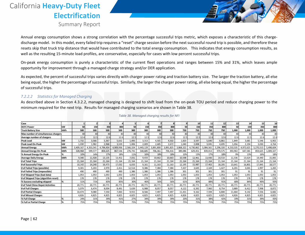
California Heavy-Duty Fleet Electrification
Summary Report
Page | 62
Annual energy consumption shows a strong correlation with the percentage successful trips metric, which exposes a characteristic of this charge-
discharge model. In this model, every failed trip requires a “reset” charge session before the next successful round trip is possible, and therefore these
resets skip that truck trip distance that would have contributed to the total energy consumption. This indicates that energy consumption results, as
well as the resulting 15-minute load profiles, are conservative, especially for cases with low percent successful trips.
On-peak energy consumption is purely a characteristic of the current fleet operations and ranges between 15% and 31%, which leaves ample
opportunity for improvement through a managed charge strategy and/or DER application.
As expected, the percent of successful trips varies directly with charger power rating and traction battery size. The larger the traction battery, all else
being equal, the higher the percentage of successful trips. Similarly, the larger the charger power rating, all else being equal, the higher the percentage
of successful trips.
7.2.2.2 Statistics for Managed Charging
As described above in Section 4.3.2.2, managed charging is designed to shift load from the on-peak TOU period and reduce charging power to the
minimum required for the next trip. Results for managed charging scenarios are shown in Table 38.
Table 38. Managed charging results for NFI
Case 1 2 3 4 5 6 7 8 9 10 11 12 13 14 15 16
DCFC Power kW 50 150 350 800 50 150 350 800 50 150 350 800 50 150 350 800
Truck Battery Size kWh 500 500 500 500 300 300 300 300 750 750 750 750 1,000 1,000 1,000 1,000
Max number of simultaneous chargers 40 40 40 40 40 40 40 40 40 40 40 40 40 40 40 40
Average number of chargers 12.4 12.5 12.6 12.6 12.5 12.5 12.6 12.6 12.5 12.5 12.6 12.6 12.6 12.5 12.6 12.6
Peak Load kW 1,732 3,566 5,367 5,632 1,495 3,313 4,501 4,502 1,820 3,597 5,640 6,861 1,849 3,681 5,546 6,902
Peak Load On-Peak kW 1,030 1,982 2,968 3,539 1,006 2,009 2,685 2,672 1,040 2,008 3,045 4,695 1,056 2,194 3,030 4,764
Annual Energy kWh 3,409,167 4,353,541 4,794,454 4,909,936 2,566,324 3,443,129 3,891,800 3,891,825 3,868,322 4,730,862 5,084,561 5,296,320 4,210,535 4,972,621 5,270,513 5,498,604
Annual Energy On-Peak kWh 328,968 599,577 804,625 867,536 276,741 540,685 706,361 706,416 389,086 629,451 839,013 970,575 393,963 647,581 859,625 1,009,327
% Annual Energy On-Peak % 10% 14% 17% 18% 11% 16% 18% 18% 10% 13% 17% 18% 9% 13% 16% 18%
Average Daily Energy kWh 9,340 11,928 13,135 13,452 7,031 9,433 10,662 10,663 10,598 12,961 13,930 14,510 11,536 13,624 14,440 15,065
# of Total Trips 21,164 21,164 21,164 21,164 21,164 21,164 21,164 21,164 21,164 21,164 21,164 21,164 21,164 21,164 21,164 21,164
# of Successful Trips 10,142 14,240 16,473 17,032 6,033 9,161 11,163 11,163 12,195 15,987 17,463 18,205 13,641 16,801 17,845 18,577
# of Failed Trips (possible) 9,301 5,203 2,970 2,411 12,514 9,386 7,384 7,384 7,437 3,645 2,169 1,427 6,201 3,041 1,997 1,265
# of Failed Trips (impossible) 490 490 490 490 1,386 1,386 1,386 1,386 301 301 301 301 91 91 91 91
# of Skipped Trips (bad data) 1,053 1,053 1,053 1,053 1,053 1,053 1,053 1,053 1,053 1,053 1,053 1,053 1,053 1,053 1,053 1,053
# of Skipped Trips (algorithm reset) 178 178 178 178 178 178 178 178 178 178 178 178 178 178 178 178
% Success excluding skipped % 51% 71% 83% 85% 30% 46% 56% 56% 61% 80% 88% 91% 68% 84% 90% 93%
# of Total Chino Depot Activities 20,771 20,771 20,771 20,771 20,771 20,771 20,771 20,771 20,771 20,771 20,771 20,771 20,771 20,771 20,771 20,771
# of Full Charges 5,079 6,474 8,004 8,491 5,639 6,988 8,057 8,057 4,122 6,392 7,960 8,754 3,889 6,412 7,998 8,872
# of Partial Charges 10,474 9,080 7,550 7,063 9,915 8,566 7,497 7,497 11,431 9,162 7,594 6,800 11,664 9,142 7,556 6,682
# of Missed Charges 4,826 4,825 4,825 4,825 4,825 4,825 4,825 4,825 4,826 4,825 4,825 4,825 4,826 4,825 4,825 4,825
% Full Charge % 24% 31% 39% 41% 27% 34% 39% 39% 20% 31% 38% 42% 19% 31% 39% 43%
% Full or Partial Charge % 75% 75% 75% 75% 75% 75% 75% 75% 75% 75% 75% 75% 75% 75% 75% 75%

California Heavy-Duty Fleet Electrification
Summary Report
Page | 63
These managed charging results include the same performance metrics as the unmanaged scenario but differ regarding energy and power
consumption, as well as the maximum number of chargers required in each scenario.
7.2.2.3 Comparison between Managed and Unmanaged Charging
The differences for all between managed and unmanaged charging are shown in Table 39.
Table 39. Comparison of managed versus unmanaged charging results for NFI
Several observations are apparent from the comparison of managed charging with unmanaged charging. First, managed charging requires both more
installed chargers (between 8% and 54% increase) and increases the average number of chargers utilized (between 31% and 392% increase) as
compared to unmanaged charging. This is largely a result of the assumption that there is no limit in the model for the maximum number of chargers
together with the fact that managed charging strategy was defined to reducing the charge power to the minimum required to charge the truck over
the available charging window. For scenarios with very high-power chargers, this approach results in the chargers typically operating at only a small
fraction of their power rating. Because the current analysis does not model the “charger sharing” approach of rotating trucks through a single charging
stall (similar to a diesel fueling station operation), the required number of chargers for scenarios with high-power chargers (350 kW and 800 kW) is
likely overstated.
Second, as expected, managed charging reduces peak load (both on-peak and all day) as well as the energy consumption during on-peak periods. This
result was expected since the charging algorithm was designed to achieve this type of result. The largest reduction in on-peak peak load was 39% for
the scenario with 800 kW charger power and 500 kWh traction battery rating, corresponding to a drop of 2.24 MW when using managed charging.
This result speaks to the high potential impact for managed charging in mitigating grid impacts and electricity costs.
It is interesting however that the scenarios with high-power chargers (350 kW and 800 kW) show a greater percent reduction in peak load and on-
peak peak load compared to the lower-power chargers, which indicates the greater potential for impact of managed charging strategy when using
high-power chargers. This is a different result than what is shown for the percent reduction in on-peak energy consumption, however, which is
more uniform across the scenarios.
Case 1 2 3 4 5 6 7 8 9 10 11 12 13 14 15 16
DCFC Power kW 50 150 350 800 50 150 350 800 50 150 350 800 50 150 350 800
Truck Battery Size kWh 500 500 500 500 300 300 300 300 750 750 750 750 1,000 1,000 1,000 1,000
Max number of simultaneous chargers 11% 38% 48% 48% 33% 38% 38% 38% 8% 38% 48% 54% 8% 38% 48% 54%
Average number of chargers 52% 189% 305% 347% 93% 226% 311% 311% 39% 178% 304% 385% 31% 173% 304% 392%
Peak Load kW -1% -14% -21% -27% -5% -16% -18% -18% -2% -14% -21% -29% -1% -12% -22% -28%
Peak Load On-Peak kW -23% -26% -36% -39% -25% -19% -34% -34% -29% -31% -34% -33% -28% -25% -35% -34%
Annual Energy kWh 0% 0% 0% 0% 0% 0% 0% 0% 0% 0% 0% 0% 0% 0% 0% 0%
Annual Energy On-Peak kWh -36% -43% -43% -42% -41% -44% -41% -41% -34% -42% -43% -41% -38% -42% -42% -41%
% Annual Energy On-Peak % -36% -43% -43% -42% -41% -44% -41% -41% -34% -42% -43% -41% -38% -42% -42% -41%
Average Daily Energy kWh 0% 0% 0% 0% 0% 0% 0% 0% 0% 0% 0% 0% 0% 0% 0% 0%

California Heavy-Duty Fleet Electrification
Summary Report
Page | 64
7.2.3 Schneider Full Charge-Discharge Model Results
7.2.3.1 Statistics for Unmanaged Charging
The full statistics for unmanaged charging for the sixteen unmanaged charging scenarios are shown in Table 40.
Table 40. Unmanaged charging results for Schneider
Similar to the NFI case, these results indicate that more chargers are needed when using a smaller charger rating since more chargers will be occupied
to meet the fleet operational need as compared to higher power chargers. The effect of a higher charger rating in reducing the number of chargers
diminishes at the greater 350 kW charger rating, compared to diminishing after the 150 kW charger rating for NFI. This may be due to the longer
average trip length for Schneider, which brings more charging windows with deeply depleted batteries that can take advantage of the higher power
charging capability compared to NFI.
Similar to NFI, peak load is consistently directly related to DCFC power rating, except when battery size is limiting (as in the scenario with 800 kW
charger rating and 300 kWh battery capacity). On-peak load generally follows this pattern as well apart from the increases from 50 kW to 150 kW
charger ratings, where on-peak loads actually decrease with increasing charger ratings. This suggests that the higher power chargers can complete
charging before on-peak periods start, whereas the 50 kW chargers continue to charge into the on-peak period.
Case 1 2 3 4 5 6 7 8 9 10 11 12 13 14 15 16
DCFC Power kW 50 150 350 800 50 150 350 800 50 150 350 800 50 150 350 800
Truck Battery Size kWh 500 500 500 500 300 300 300 300 750 750 750 750 1,000 1,000 1,000 1,000
Max number of simultaneous chargers 32 24 18 17 28 22 18 18 33 25 20 17 33 25 21 17
Average number of chargers 10.6 4.7 2.9 2.5 7.6 3.6 2.6 2.6 12.0 5.6 3.3 2.4 12.8 5.9 3.4 2.4
Peak Load kW 1,632 3,161 4,504 5,485 1,467 2,480 3,489 3,489 1,709 3,524 5,472 7,650 1,706 3,600 5,696 8,093
Peak Load On-Peak kW 1,507 993 1,842 2,105 696 800 1,263 1,263 1,604 1,263 1,867 3,053 1,632 1,579 1,846 3,144
Annual Energy kWh 4,601,380 4,758,298 4,769,590 4,771,743 3,026,678 3,052,430 3,058,989 3,058,989 5,383,515 6,164,940 6,179,089 6,184,477 5,821,282 6,760,850 6,773,706 6,778,601
Annual Energy On-Peak kWh 824,220 478,198 498,465 505,768 351,561 319,595 331,440 331,440 1,157,923 637,008 630,088 648,425 1,227,941 743,588 685,543 702,610
% Annual Energy On-Peak % 18% 10% 10% 11% 12% 10% 11% 11% 22% 10% 10% 10% 21% 11% 10% 10%
Average Daily Energy kWh 12,607 13,036 13,067 13,073 8,292 8,363 8,381 8,381 14,749 16,890 16,929 16,944 15,949 18,523 18,558 18,572
# of Total Trips 9,475 9,475 9,475 9,475 9,475 9,475 9,475 9,475 9,475 9,475 9,475 9,475 9,475 9,475 9,475 9,475
# of Successful Trips 2,750 3,044 3,068 3,074 1,022 1,070 1,089 1,089 4,458 6,313 6,344 6,359 5,717 8,358 8,390 8,398
# of Failed Trips (possible) 345 51 27 21 88 40 21 21 1,921 66 35 20 2,698 57 25 17
# of Failed Trips (impossible) 6,378 6,378 6,378 6,378 8,363 8,363 8,363 8,363 3,094 3,094 3,094 3,094 1,058 1,058 1,058 1,058
# of Skipped Trips (bad data) - - - - - - - - - - - - - - - -
# of Skipped Trips (algorithm reset) 2 2 2 2 2 2 2 2 2 2 2 2 2 2 2 2
% Success excluding skipped % 29% 32% 32% 32% 11% 11% 11% 11% 47% 67% 67% 67% 60% 88% 89% 89%
# of Total Chino Depot Activities 9,514 9,514 9,514 9,514 9,514 9,514 9,514 9,514 9,514 9,514 9,514 9,514 9,514 9,514 9,514 9,514
# of Full Charges 6,085 9,252 9,324 9,331 8,921 9,295 9,328 9,328 3,430 9,176 9,315 9,336 3,198 9,123 9,308 9,337
# of Partial Charges 3,429 262 190 183 593 219 186 186 6,084 338 199 178 6,316 391 206 177
# of Missed Charges - - - - - - - - - - - - - - - -
% Full Charge % 64% 97% 98% 98% 94% 98% 98% 98% 36% 96% 98% 98% 34% 96% 98% 98%
% Full or Partial Charge % 100% 100% 100% 100% 100% 100% 100% 100% 100% 100% 100% 100% 100% 100% 100% 100%

California Heavy-Duty Fleet Electrification
Summary Report
Page | 65
Similar to NFI, annual energy consumption shows a strong correlation with the percentage successful trips metric, a reminder of the skipped trips
characteristic of this charge-discharge model and the resulting effect on energy consumption.
On-peak energy consumption is purely a characteristic of the current fleet operations and ranges between 10% and 22%, which leaves ample
opportunity for improvement through a managed charge strategy and/or DER application. This is a lower percentage of on-peak charging compared
to NFI and perhaps indicates that the Schneider fleet has generally less dwell time at the depot and thus less charging during on-peak TOU periods.
As expected, the percent of successful trips varies directly with charger power rating and traction battery size. Similar to NFI, the larger the traction
battery, all else being equal, the higher the percentage of successful trips. Different from NFI, increasing charger power rating, while holding battery
size equal, only increases percent success when going from 50kW to 150 kW charger rating. For higher charger ratings, the effect tails off, and
increasing charger rating barely impacts the percent success; this characteristic appears across traction battery sizes. The explanation is likely related
to the longer charging windows for the Schneider fleet, making the results fairly insensitive to increased charging power. In other words, higher power
charging is more important when there are limits on the time available for charging.
7.2.3.2 Statistics for Managed Charging
As described above in Section 4.3.2.2, managed charging is designed to shift load from the on-peak TOU period and reduce charging power to the
minimum required for the next trip. Results for managed charging scenarios are shown as
.

California Heavy-Duty Fleet Electrification
Summary Report
Page | 66
Table 41. Managed Charging Results for Schneider
These managed charging results include the same performance metrics as the unmanaged scenario but differ regarding energy and power
consumption, as well as the maximum number of chargers required in each scenario.
7.2.3.3 Comparison between Managed and Unmanaged Charging
The differences for all between managed and unmanaged charging are shown in Table 42.
Table 42. Comparison of Managed and Unmanaged Charging for Schneider
Case 1 2 3 4 5 6 7 8 9 10 11 12 13 14 15 16
DCFC Power kW 50 150 350 800 50 150 350 800 50 150 350 800 50 150 350 800
Truck Battery Size kWh 500 500 500 500 300 300 300 300 750 750 750 750 1,000 1,000 1,000 1,000
Max number of simultaneous chargers 36 35 35 34 35 35 34 34 35 35 35 34 35 35 35 34
Average number of chargers 13.3 10.3 9.9 9.8 11.5 10.0 9.8 9.8 13.4 10.6 10.0 9.8 13.5 10.8 10.0 9.8
Peak Load kW 1,726 2,814 3,573 3,843 1,453 2,035 2,344 2,338 1,905 3,380 4,130 4,920 2,066 3,619 4,464 5,244
Peak Load On-Peak kW 1,359 452 563 716 421 274 430 428 1,531 611 654 1,075 1,544 1,111 656 1,129
Annual Energy kWh 4,635,927 4,763,873 4,770,510 4,772,482 3,035,989 3,056,406 3,060,295 3,060,297 5,388,352 6,169,241 6,180,271 6,184,325 5,821,237 6,762,685 6,775,168 6,778,176
Annual Energy On-Peak kWh 659,425 100,922 49,992 42,349 228,704 41,607 28,591 28,595 796,139 233,522 72,763 52,413 815,018 368,151 87,062 57,167
% Annual Energy On-Peak % 14% 2% 1% 1% 8% 1% 1% 1% 15% 4% 1% 1% 14% 5% 1% 1%
Average Daily Energy kWh 12,701 13,052 13,070 13,075 8,318 8,374 8,384 8,384 14,763 16,902 16,932 16,943 15,949 18,528 18,562 18,570
# of Total Trips 9,475 9,475 9,475 9,475 9,475 9,475 9,475 9,475 9,475 9,475 9,475 9,475 9,475 9,475 9,475 9,475
# of Successful Trips 2,810 3,063 3,076 3,077 1,049 1,086 1,094 1,094 4,479 6,334 6,352 6,362 5,731 8,374 8,398 8,402
# of Failed Trips (possible) 285 32 19 18 61 24 16 16 1,900 45 27 17 2,684 41 17 13
# of Failed Trips (impossible) 6,378 6,378 6,378 6,378 8,363 8,363 8,363 8,363 3,094 3,094 3,094 3,094 1,058 1,058 1,058 1,058
# of Skipped Trips (bad data) - - - - - - - - - - - - - - - -
# of Skipped Trips (algorithm reset) 2 2 2 2 2 2 2 2 2 2 2 2 2 2 2 2
% Success excluding skipped % 30% 32% 32% 32% 11% 11% 12% 12% 47% 67% 67% 67% 60% 88% 89% 89%
# of Total Chino Depot Activities 9,514 9,514 9,514 9,514 9,514 9,514 9,514 9,514 9,514 9,514 9,514 9,514 9,514 9,514 9,514 9,514
# of Full Charges 6,914 9,359 9,412 9,418 9,106 9,392 9,414 9,414 3,579 9,302 9,410 9,425 3,248 9,269 9,410 9,425
# of Partial Charges 2,600 155 102 96 408 122 100 100 5,935 212 104 89 6,266 245 104 89
# of Missed Charges - - - - - - - - - - - - - - - -
% Full Charge % 73% 98% 99% 99% 96% 99% 99% 99% 38% 98% 99% 99% 34% 97% 99% 99%
% Full or Partial Charge % 100% 100% 100% 100% 100% 100% 100% 100% 100% 100% 100% 100% 100% 100% 100% 100%
Case 1 2 3 4 5 6 7 8 9 10 11 12 13 14 15 16
DCFC Power kW 50 150 350 800 50 150 350 800 50 150 350 800 50 150 350 800
Truck Battery Size kWh 500 500 500 500 300 300 300 300 750 750 750 750 1,000 1,000 1,000 1,000
Max number of simultaneous chargers 13% 46% 94% 100% 25% 59% 89% 89% 6% 40% 75% 100% 6% 40% 67% 100%
Average number of chargers 25% 118% 241% 293% 51% 178% 278% 278% 12% 90% 202% 308% 6% 84% 193% 308%
Peak Load kW 6% -11% -21% -30% -1% -18% -33% -33% 11% -4% -25% -36% 21% 1% -22% -35%
Peak Load On-Peak kW -10% -54% -69% -66% -40% -66% -66% -66% -5% -52% -65% -65% -5% -30% -64% -64%
Annual Energy kWh 1% 0% 0% 0% 0% 0% 0% 0% 0% 0% 0% 0% 0% 0% 0% 0%
Annual Energy On-Peak kWh -20% -79% -90% -92% -35% -87% -91% -91% -31% -63% -88% -92% -34% -50% -87% -92%
% Annual Energy On-Peak % -21% -79% -90% -92% -37% -86% -92% -92% -33% -62% -88% -92% -33% -51% -87% -92%
Average Daily Energy kWh 1% 0% 0% 0% 0% 0% 0% 0% 0% 0% 0% 0% 0% 0% 0% 0%

California Heavy-Duty Fleet Electrification
Summary Report
Page | 67
Several observations are drawn from the comparison of managed charging with unmanaged charging. Similar to NFI, managed charging requires both
more installed chargers (between 6% and 100% increase) and increases the average number of chargers utilized (between 6% and 308% increase) as
compared to unmanaged charging. Again, this is largely a result of the assumption that there is no limit in the model for the maximum number of
chargers together with the fact that managed charging strategy was defined to reducing the charge power to the minimum required to charge the
truck over the available charging window. For scenarios with very high-power chargers, this approach results in the chargers typically operating at only
a small fraction of their power rating. Because the current analysis does not model the “charger sharing” approach of rotating trucks through a single
charging stall (similar to a diesel fueling station operation), the required number of chargers for scenarios with high-power chargers (350 kW and 800
kW) is likely overstated.
Second, and also similar to NFI, managed charging reduces peak load (both on-peak and all day) as well as the energy consumption during on-peak
periods. This result was expected since the charging algorithm was designed to achieve this type of result. Noteworthy are the scenarios where
managed charging almost eliminates on-peak charging with reductions up to 92%. The largest reduction in on-peak peak load was 69% for the
scenario with 350 kW charger power and 500 kWh traction battery rating, corresponding to a drop of 1.28 MW when using managed charging. These
results speak to the high potential impact for managed charging in mitigating grid impacts and electricity costs.
Also similar to NFI, the scenarios with high-power chargers (350 kW and 800 kW) show a greater percent reduction in peak load and on-peak peak
load compared to the lower-power chargers, which indicates the greater potential for impact of managed charging strategy when using high-power
chargers. Also, the percent reduction in on-peak energy consumption remains more uniform across the scenarios.