homological algebra - reed collegepeople.reed.edu/~iswanson/homologicalalgebra.pdf · homological...
TRANSCRIPT
Homological Algebra
Irena Swanson, Rome, Spring 2010
This is work in progress. I am still adding, subtracting, modifying. Any comments
are welcome.
These lecture notes were delivered at University Roma Tre between March and May
2010. I was invited by Professor Stefania Gabelli and funded by INDAM. I am grateful to
Stefania, to INDAM, and to the students.
The goal of these lectures is to introduce homological algebra to the students whose
commutative algebra background consists mostly of the material in Atiyah-MacDonald [1].
Homological algebra is a rich area and can be studied quite generally; in the first few lectures
I tried to be quite general, using groups or left modules over not necessarily commutative
rings, but in these notes and also in most of the lectures, the subject matter was mostly
modules over commutative rings. Much in these notes is from the course I took from Craig
Huneke in 1989.
Table of contents:
Section 1: Overview, background, and definitions 2
Section 2: Projective modules 12
Section 3: Projective, flat, free resolutions 16
Section 4: General manipulations of complexes 20
Section 5: More on Koszul complexes 23
Section 6: General manipulations applied to projective resolutions 25
Section 7: Tor 27
Section 8: Regular rings, part I 31
Section 9: Review of Krull dimension 32
Section 10: Regular sequences 37
Section 11: Regular sequences and Tor 41
Section 12: Cohen–Macaulay rings and modules 44
Section 13: Regular rings, part II 46
Section 14: Injective and divisible modules 50
Section 15: Injective resolutions 54
Section 16: A definition of Ext using injective resolutions 57
Section 17: A definition of Ext using projective resolutions 58
Section 18: The two definitions of Ext are isomorphic 60
Section 19: Ext and extensions 61
Section 20: Essential extensions 65
1
Section 21: Structure of injective modules 69
Section 22: Duality and injective hulls 71
Section 23: More on injective resolutions 74
Section 24: Gorenstein rings 79
Section 25: Bass numbers 82
Section 26: Criteria for exactness 83
Bibliography 88
1 Overview, background, and definitions
1. What is a complex? A complex is a collection of groups (or left modules) and ho-
momorphisms, usually written in the following way:
· · · →Mi+1di+1−→ Mi
di−→ Mi−1 → · · · ,
where the Mi are groups (or left modules), the di are group (or left module) homomor-
phisms, and for all i, di ◦ di+1 = 0. Rather than write out the whole complex, we will
typically abbreviate it as C•, M• or (M•, d•), et cetera, where the dot differentiates the
complex from a module, and d• denotes the collection of all the di.
A complex is bounded below if Mi = 0 for all sufficiently small (negative) i; a
complex is bounded above if Mi = 0 for all sufficiently large (positive) i; a complex is
bounded if Mi = 0 for all sufficiently large |i|.A complex is exact at the ith place if ker(di) = im(di+1). A complex is exact if it
is exact at all places.
A complex is free (resp. flat, projective, injective) if all the Mi are free (resp. flat,
projective, injective).
A complex is called a short exact sequence if it is an exact complex of the form
0 →M ′i−→ M
p−→ M ′′ → 0.
A long exact sequence is simply an exact complex that may be longer but is not nec-
essarily longer; typically long exact sequences arise in some natural way from short exact
sequences (see Theorem 4.4).
2
Remark 1.1 Note that every long exact sequence
· · · →Mi+1di+1−→ Mi
di−→ Mi−1 → · · ·
decomposes into short exact sequences
0 → ker di−1 → Mi−1 → im di−1 → 0||
0 → ker di → Mi → imdi → 0||
0 → ker di+1 →Mi+1 → im di+1 → 0,
et cetera.
We will often write only parts of complexes, such as for exampleM3 →M2 →M1 → 0,
and we will say that such a (fragment of a) complex is exact if there is exactness at a module
that has both an incoming and an outgoing map.
2. Homology of a complex C•. The nth homology group (or module) is
Hn(C•) =ker dnim dn+1
.
3. Cocomplexes. A complex might be naturally numbered in the opposite order:
C• : · · · →M i−1 di−1
−→ M i di
−→ M i+1 → · · · ,
in which case we index the groups (or modules) and the homomorphisms with superscripts
rather than the subscripts, and we call it a cocomplex. The nth cohomology module
of such a cocomplex C• is
Hn(C•) =ker dn
im dn−1.
4. Free and projective resolutions. LetM be an R-module. A free (resp. projective)
resolution of M is a complex
· · · → Fi+1di+1−→ Fi
di−→ Fi−1 → · · · → F1d1−→ F0 → 0,
where the Fi are free (resp. projective) modules over R (definition of projective modules is
in Section 2) and where
· · · → Fi+1di+1−→ Fi
di−→ Fi−1 → · · · −→ F1d1−→ F0 →M → 0
is exact. Free, projective, flat resolutions are not uniquely determined, in the sense that
the free modules and the homomorphisms are not uniquely defined, not even up to iso-
morphisms. Namely, to construct a free resolution, we use the fact that every module is a
3
homomorphic image of a free module. Thus we may take F0 to be a free module that maps
onto M , and we have non-isomorphic choices there; we then take F1 to be a free module
that maps onto the kernel of F0 → M , giving an exact complex F1 → F0 →M → 0; after
which we may take F2 to be a free module that maps onto the kernel of F1 → F0, et cetera.
Note: sometimes, mostly in order to save writing time, · · · → Fi+1 → Fi → Fi−1 →· · · → F1 → F0 →M → 0 is also called a free (resp. projective) resolution of M .
5. Injective resolutions. Let M be an R-module. An injective resolution of M is a
cocomplex
0 → I0 → I1 → I2 → I3 → · · · ,
where the In are injective modules over R (definition of injective modules is in Section 21)
and where
0 →M → I0 → I1 → I2 → I3 → · · ·
is exact. Also injective resolutions are not uniquely determined, and we sometimes call the
latter exact cocomplex an injective resolution.
6. Other ways to make complexes. Let C• = · · · → Cndn−→ Cn−1
dn−1−→ Cn−2 → · · · bea complex of R-modules.
(1) Homology complex: We can immediately form the trivial complexH(C•), wherethe nth module is Hn(C•), and all the complex maps are zero (which we may want
to think of as the maps induced by the original complex maps).
If M is an R-module, we can form the following natural complexes:
(2) Tensor product:
C• ⊗R M : · · · → Cn ⊗R Mdn⊗id−−−→ Cn−1 ⊗R M
dn−1⊗id−−−→ Cn−2 ⊗R M → · · · .
It is straightforward to verify that this is still a complex.
(3) Hom from M, denoted HomR(M,C•), is:
· · · → Hom(M,Cn)Hom(M,dn)−−−→ HomR(M,Cn−1)
Hom(M,dn−1)−−−−−−→ HomR(M,Cn−2) → · · · ,
where Hom(M, dn) = dn ◦ . It is straightforward to verify that this is still a
complex.
(4) Hom into M, denoted HomR(C•,M), is:
· · · → Hom(Cn+1,M)Hom(dn,M)−−−→ HomR(Cn,M)
Hom(dn+1,M)−−−−−−→ HomR(Cn+1,M) → · · · ,
where Hom(dn,M) = ◦ dn. It is straightforward to verify that this is now a
cocomplex.
4
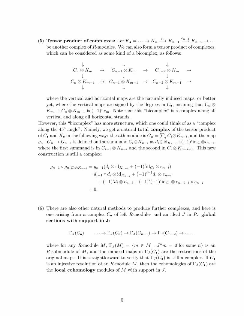
(5) Tensor product of complexes: LetK• = · · · → Knen−→ Kn−1
en−1−→ Kn−2 → · · ·be another complex of R-modules. We can also form a tensor product of complexes,
which can be considered as some kind of a bicomplex, as follows:
↓ ↓ ↓Cn ⊗Km → Cn−1 ⊗Km → Cn−2 ⊗Km →
↓ ↓ ↓Cn ⊗Km−1 → Cn−1 ⊗Km−1 → Cn−2 ⊗Km−1 →
↓ ↓ ↓
where the vertical and horizontal maps are the naturally induced maps, or better
yet, where the vertical maps are signed by the degrees in C•, meaning that Cn ⊗Km → Cn ⊗Km−1 is (−1)nem. Note that this “bicomplex” is a complex along all
vertical and along all horizontal strands.
However, this “bicomplex” has more structure, which one could think of as a “complex
along the 45◦ angle”. Namely, we get a natural total complex of the tensor product
of C• andK• in the following way: the nth module is Gn =∑
i Ci⊗Kn−i, and the map
gn : Gn → Gn−1 is defined on the summand Ci⊗Kn−i as di⊗idKn−i+(−1)iidCi
⊗en−i,where the first summand is in Ci−1 ⊗Kn−i and the second in Ci ⊗Kn−i−1. This newconstruction is still a complex:
gn−1 ◦ gn|Ci⊗Kn−i= gn−1(di ⊗ idKn−i
+ (−1)iidCi⊗ en−i)
= di−1 ◦ di ⊗ idKn−i+ (−1)i−1di ⊗ en−i
+ (−1)idi ⊗ en−i + (−1)i(−1)iidCi⊗ en−i−1 ◦ en−i
= 0.
(6) There are also other natural methods to produce further complexes, and here is
one arising from a complex C• of left R-modules and an ideal J in R: global
sections with support in J:
ΓJ (C•) · · · → ΓJ (Cn) → ΓJ (Cn−1) → ΓJ(Cn−2) → · · · ,
where for any R-module M , ΓJ(M) = {m ∈ M : Jnm = 0 for some n} is an
R-submodule of M , and the induced maps in ΓJ(C•) are the restrictions of the
original maps. It is straightforward to verify that ΓJ(C•) is still a complex. If C•is an injective resolution of an R-module M , then the cohomologies of ΓJ(C•) arethe local cohomology modules of M with support in J .
5
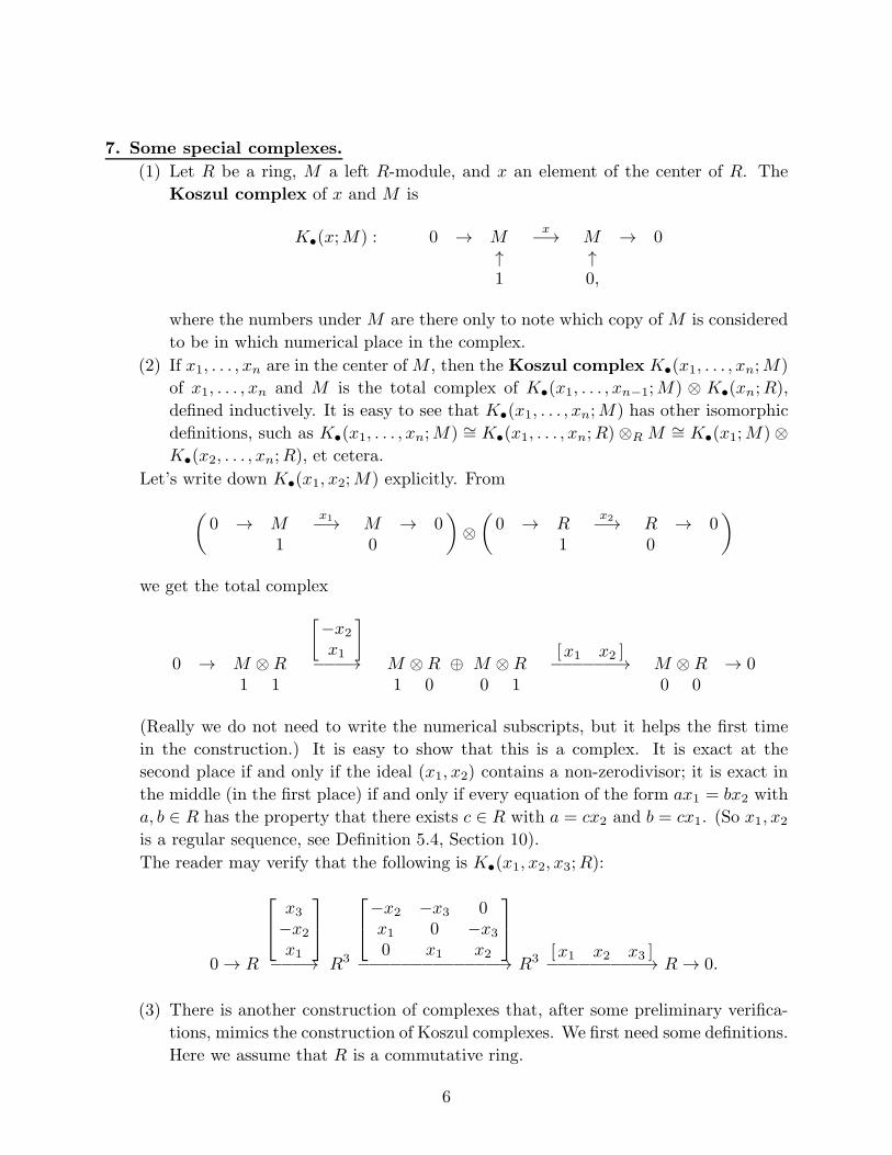
7. Some special complexes.
(1) Let R be a ring, M a left R-module, and x an element of the center of R. The
Koszul complex of x and M is
K•(x;M) : 0 → Mx−→ M → 0
↑ ↑1 0,
where the numbers under M are there only to note which copy of M is considered
to be in which numerical place in the complex.
(2) If x1, . . . , xn are in the center ofM , then the Koszul complex K•(x1, . . . , xn;M)
of x1, . . . , xn and M is the total complex of K•(x1, . . . , xn−1;M) ⊗ K•(xn;R),defined inductively. It is easy to see that K•(x1, . . . , xn;M) has other isomorphic
definitions, such as K•(x1, . . . , xn;M) ∼= K•(x1, . . . , xn;R)⊗R M ∼= K•(x1;M)⊗K•(x2, . . . , xn;R), et cetera.
Let’s write down K•(x1, x2;M) explicitly. From
(0 → M
x1−→ M → 01 0
)⊗(0 → R
x2−→ R → 01 0
)
we get the total complex
0 → M ⊗ R
[−x2x1
]
−−−→ M ⊗R ⊕ M ⊗ R[x1 x2 ]−−−−−−→ M ⊗ R → 0
1 1 1 0 0 1 0 0
(Really we do not need to write the numerical subscripts, but it helps the first time
in the construction.) It is easy to show that this is a complex. It is exact at the
second place if and only if the ideal (x1, x2) contains a non-zerodivisor; it is exact in
the middle (in the first place) if and only if every equation of the form ax1 = bx2 with
a, b ∈ R has the property that there exists c ∈ R with a = cx2 and b = cx1. (So x1, x2is a regular sequence, see Definition 5.4, Section 10).
The reader may verify that the following is K•(x1, x2, x3;R):
0 → R
x3−x2x1
−−−→ R3
−x2 −x3 0x1 0 −x30 x1 x2
−−−−−−−−−−−−−→ R3 [x1 x2 x3 ]−−−−−−−−−→ R → 0.
(3) There is another construction of complexes that, after some preliminary verifica-
tions, mimics the construction of Koszul complexes. We first need some definitions.
Here we assume that R is a commutative ring.
6
If M is an R-module, we define the n-fold tensor product of M to be denoted
M⊗n: M⊗1 = M , M⊗2 = M ⊗M , and in general for n ≥ 1, M⊗(n+1) = M⊗n ⊗M .
It is sensible to define M⊗0 = R.
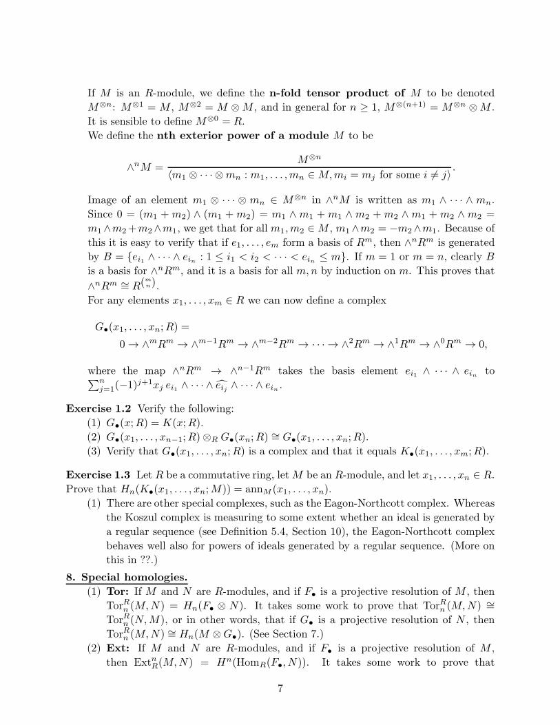
We define the nth exterior power of a module M to be
∧nM =M⊗n
〈m1 ⊗ · · · ⊗mn : m1, . . . , mn ∈M,mi = mj for some i 6= j〉 .
Image of an element m1 ⊗ · · · ⊗ mn ∈ M⊗n in ∧nM is written as m1 ∧ · · · ∧ mn.
Since 0 = (m1 +m2) ∧ (m1 +m2) = m1 ∧m1 +m1 ∧m2 +m2 ∧m1 +m2 ∧m2 =
m1∧m2+m2∧m1, we get that for all m1, m2 ∈M , m1∧m2 = −m2∧m1. Because of
this it is easy to verify that if e1, . . . , em form a basis of Rm, then ∧nRm is generated
by B = {ei1 ∧ · · · ∧ ein : 1 ≤ i1 < i2 < · · · < ein ≤ m}. If m = 1 or m = n, clearly B
is a basis for ∧nRm, and it is a basis for all m,n by induction on m. This proves that
∧nRm ∼= R(m
n).
For any elements x1, . . . , xm ∈ R we can now define a complex
G•(x1, . . . , xn;R) =
0 → ∧mRm → ∧m−1Rm → ∧m−2Rm → · · · → ∧2Rm → ∧1Rm → ∧0Rm → 0,
where the map ∧nRm → ∧n−1Rm takes the basis element ei1 ∧ · · · ∧ ein to∑nj=1(−1)j+1xj ei1 ∧ · · · ∧ eij ∧ · · · ∧ ein .
Exercise 1.2 Verify the following:
(1) G•(x;R) = K(x;R).
(2) G•(x1, . . . , xn−1;R)⊗R G•(xn;R) ∼= G•(x1, . . . , xn;R).(3) Verify that G•(x1, . . . , xn;R) is a complex and that it equals K•(x1, . . . , xm;R).
Exercise 1.3 Let R be a commutative ring, letM be an R-module, and let x1, . . . , xn ∈ R.Prove that Hn(K•(x1, . . . , xn;M)) = annM (x1, . . . , xn).
(1) There are other special complexes, such as the Eagon-Northcott complex. Whereas
the Koszul complex is measuring to some extent whether an ideal is generated by
a regular sequence (see Definition 5.4, Section 10), the Eagon-Northcott complex
behaves well also for powers of ideals generated by a regular sequence. (More on
this in ??.)
8. Special homologies.
(1) Tor: If M and N are R-modules, and if F• is a projective resolution of M , then
TorRn (M,N) = Hn(F• ⊗ N). It takes some work to prove that TorRn (M,N) ∼=TorRn (N,M), or in other words, that if G• is a projective resolution of N , then
TorRn (M,N) ∼= Hn(M ⊗G•). (See Section 7.)
(2) Ext: If M and N are R-modules, and if F• is a projective resolution of M ,
then ExtnR(M,N) = Hn(HomR(F•, N)). It takes some work to prove that
7
ExtnR(M,N) ∼= Hn(HomR(M, I•)), where I• is an injective resolution of N . (See
Section 17.)
(3) Local cohomology: If M is an R-module and J is an ideal in R, then the nth
local cohomology of M with respect to J is HnJ (M) = Hn(ΓJ(I)), where I• is an
injective resolution of M . (See ??? Time?)
9. Why study homological algebra? This is very brief, as I hope that the rest of the
course justifies the study of this material. Exactness and non-exactness of certain complexes
yields information on whether a ring in question is regular, Cohen–Macaulay, Gorenstein,
what its dimensions (Krull, projective, injective, etc.) are, and so on. While one has
other tools to determine such non-singularity properties, homological algebra is often an
excellent, convenient, and sometimes the best tool.
10. How does one determine exactness of a (part of a) complex? We list here a
few answers, starting with fairly vague ones:
(1) From theoretical aspects as above;
(2) after a concrete computation;
(3) Buchsbaum-Eisenbud criterion (see ??);
(4) knowledge of special complexes, such as Koszul complexes, the Hilbert-Burch com-
plex (see Exercise 1.10)...;
(5) and a more concrete tool/answer: the Snake Lemma. We state below two versions.
Proofs require some diagram chasing, and we leave it to the reader.
Lemma 1.4 (Snake Lemma, version I) Assume that the rows in the following com-
mutative diagram are exact and that β and δ are isomorphisms:
Aa→ B
b→ Cc→ D
d→ E↓α ↓β ↓γ ↓δ ↓ǫA′
a′
→ B′b′→ C ′
c′→ D′d′
→ E′.
Then if ǫ is injective, γ is surjective; and if ǫ is surjective, γ is injective.
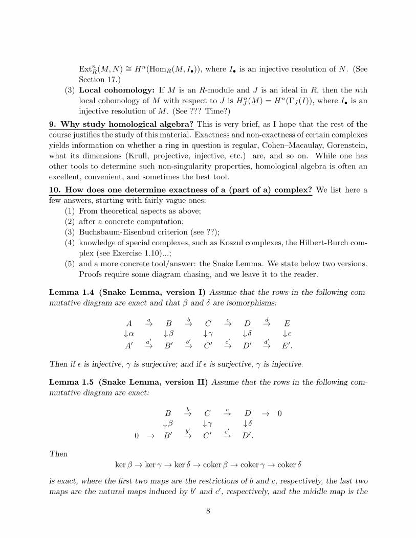
Lemma 1.5 (Snake Lemma, version II) Assume that the rows in the following com-
mutative diagram are exact:
Bb→ C
c→ D → 0↓β ↓γ ↓δ
0 → B′b′→ C ′
c′→ D′.
Then
ker β → ker γ → ker δ → cokerβ → coker γ → coker δ
is exact, where the first two maps are the restrictions of b and c, respectively, the last two
maps are the natural maps induced by b′ and c′, respectively, and the middle map is the
8
so-called connecting homomorphism. We describe this homomorphism here explicitly:
let x ∈ ker δ. Since c is surjective, there exists y ∈ C such that x = c(y). Since the diagram
commutes, c′γy = δcy = δx = 0, so that γy ∈ ker c′ = im b′. Thus γy = b′(z) for some
z ∈ B′. Then the connecting homomorphism takes x to the image of z in cokerβ. A reader
should verify that this is a well-defined map. But this version of the Snake Lemma says
even more: If b is injective, so is ker β → ker γ; and if c′ is surjective, so is coker γ → coker δ.
11. Minimal free resolutions In certain contexts one can talk about a free resolution
with certain minimal conditions. Namely, while constructing the free resolution (see 4.
above), we may want to choose at each step a free module with a minimal number of
generators. If at each step we choose a minimal such generating set, we get a resolution of
the form
· · · → Rb2 → Rb1 → Rb0 →M → 0.
The number bi is called the ith Betti number of M . (See Exercise 3.7 to see that these
are well-defined.)
If R is a polynomial ring k[x1, . . . , xn] in variables x1, . . . , xn over a field k, and if
M is a finitely generated R-module generated by homogeneous elements, we may even
choose all the generators of all the kernels in the construction of a free resolution to be
homogeneous as well. In this case, we may make a finer partition of each bi, as follows. We
already know that M is minimally generated by b0 homogeneous elements, but these b0elements can be the union of sets of b0j elements of degree j. So we write Rb0 more finely
as ⊕jRb0j [−j], where [−j] indicates a shift in the grading. Thus with this shift, the natural
map ⊕jRb0j [−j] → M even has degree 0, i.e., the chosen homogeneous basis elements of
a certain degree map to a homogeneous element of M of the same degree. Once we have
rewritten Rbi with the finer grading, then a minimal homogeneous generating set of the
kernel can be also partitioned into its degrees, so that we can rewrite eachRbi as⊕jRbij [−j].
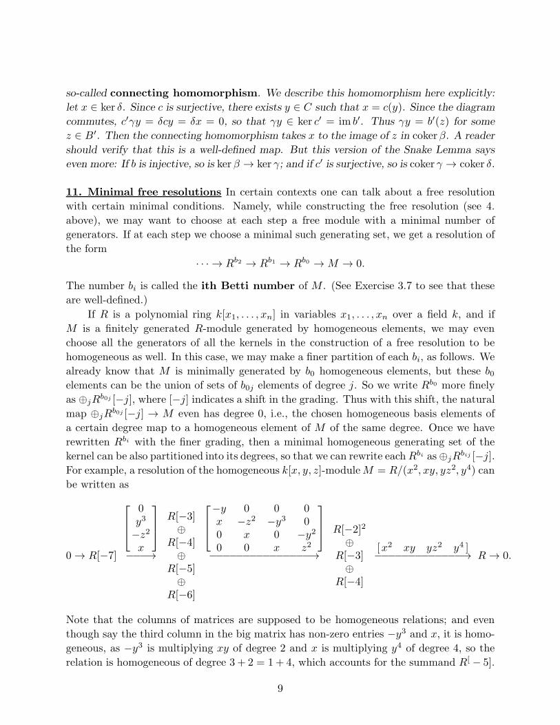
For example, a resolution of the homogeneous k[x, y, z]-moduleM = R/(x2, xy, yz2, y4) can
be written as
0 → R[−7]
0y3
−z2x
−−−→
R[−3]⊕
R[−4]⊕
R[−5]⊕
R[−6]
−y 0 0 0x −z2 −y3 00 x 0 −y20 0 x z2
−−−−−−−−−−−−−−−→
R[−2]2
⊕R[−3]⊕
R[−4]
[x2 xy yz2 y4 ]−−−−−−−−−−−−−→ R→ 0.
Note that the columns of matrices are supposed to be homogeneous relations; and even
though say the third column in the big matrix has non-zero entries −y3 and x, it is homo-
geneous, as −y3 is multiplying xy of degree 2 and x is multiplying y4 of degree 4, so the
relation is homogeneous of degree 3 + 2 = 1 + 4, which accounts for the summand R[ − 5].
9
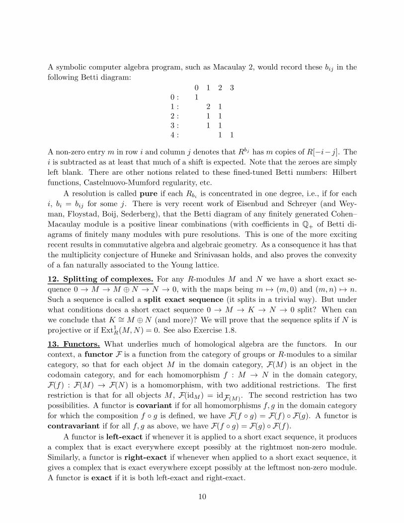
A symbolic computer algebra program, such as Macaulay 2, would record these bij in the
following Betti diagram:
0 1 2 30 : 11 : 2 12 : 1 13 : 1 14 : 1 1
A non-zero entry m in row i and column j denotes that Rbj has m copies of R[−i− j]. Thei is subtracted as at least that much of a shift is expected. Note that the zeroes are simply
left blank. There are other notions related to these fined-tuned Betti numbers: Hilbert
functions, Castelnuovo-Mumford regularity, etc.
A resolution is called pure if each Rbi is concentrated in one degree, i.e., if for each
i, bi = bij for some j. There is very recent work of Eisenbud and Schreyer (and Wey-
man, Floystad, Boij, Sederberg), that the Betti diagram of any finitely generated Cohen–
Macaulay module is a positive linear combinations (with coefficients in Q+ of Betti di-
agrams of finitely many modules with pure resolutions. This is one of the more exciting
recent results in commutative algebra and algebraic geometry. As a consequence it has that
the multiplicity conjecture of Huneke and Srinivasan holds, and also proves the convexity
of a fan naturally associated to the Young lattice.
12. Splitting of complexes. For any R-modules M and N we have a short exact se-
quence 0 → M → M ⊕ N → N → 0, with the maps being m 7→ (m, 0) and (m,n) 7→ n.
Such a sequence is called a split exact sequence (it splits in a trivial way). But under
what conditions does a short exact sequence 0 → M → K → N → 0 split? When can
we conclude that K ∼= M ⊕N (and more)? We will prove that the sequence splits if N is
projective or if Ext1R(M,N) = 0. See also Exercise 1.8.
13. Functors. What underlies much of homological algebra are the functors. In our
context, a functor F is a function from the category of groups or R-modules to a similar
category, so that for each object M in the domain category, F(M) is an object in the
codomain category, and for each homomorphism f : M → N in the domain category,
F(f) : F(M) → F(N) is a homomorphism, with two additional restrictions. The first
restriction is that for all objects M , F(idM ) = idF(M). The second restriction has two
possibilities. A functor is covariant if for all homomorphisms f, g in the domain category
for which the composition f ◦ g is defined, we have F(f ◦ g) = F(f) ◦ F(g). A functor is
contravariant if for all f, g as above, we have F(f ◦ g) = F(g) ◦ F(f).A functor is left-exact if whenever it is applied to a short exact sequence, it produces
a complex that is exact everywhere except possibly at the rightmost non-zero module.
Similarly, a functor is right-exact if whenever when applied to a short exact sequence, it
gives a complex that is exact everywhere except possibly at the leftmost non-zero module.
A functor is exact if it is both left-exact and right-exact.
10
It is easy to verify that a covariant functor F is left-exact if and only if 0 → F(A) →F(B) → F(C) is exact for every exact complex 0 → A → B → C. A covariant functor Fis right-exact if and only if F(A) → F(B) → F(C) → 0 is exact for every exact complex
A → B → C → 0. A contravariant functor F is left-exact if and only if 0 → F(C) →F(B) → F(A) is exact for every exact complex A → B → C → 0. A contravariant
functor F is right-exact if and only if F(C) → F(B) → F(A) → 0 is exact for every exact
complex 0 → A→ B → C.
We have seen some functors: HomR(M, ), HomR( ,M),M⊗R , ΓJ( ), ∧n( ). Verify
that these are functors, determine which ones are covariant, and determine their exactness
properties (see Exercise 1.7).
Definition 1.6 An R-module M is flat if M ⊗R is exact.
Thus by Exercise 1.7 below, M is flat if and only if f ⊗ idM is injective whenever f is
injective.
Exercise 1.7 Let R be a ring and M a left R-module.
(1) Prove that HomR(M, ) and HomR( ,M) are left-exact.
(2) Prove that M ⊗R is right-exact.
(3) Determine the exactness properties of ΓJ( ).
Exercise 1.8 Let 0 → M1g→ M2
h→ M3 → 0 be a short exact sequence of R-modules.
Under what conditions are any of these equivalent?
(1) There exists f :M3 →M2 such that hf = 1M3.
(2) There exists e :M2 →M1 such that eg = 1M1.
(3) M2∼=M3 ⊕M1.
Exercise 1.9 Let R be a domain and I a non-zero ideal such that for some n,m ∈ N,
Rn ∼= Rm ⊕ I . The goal is to prove that I is free. By localization we know that m+1 = n.
(1) Let 0 → Rn−1 A→ Rn → I → 0 be a short exact sequence. (Why does it exist?)
Let dj be (−1)j times the determinant of the submatrix of A obtained by deleting
the jth row. Let d be the transpose of the vector [d1, . . . , dn]. Prove that Ad = 0.
(2) Define a map g from I to the ideal generated by all the di sending the image of a
basis vector of Rn to dj. Prove that g is a well-defined homomorphism.
(3) Prove that I ∼= (d1, . . . , dn).
(4) Prove that (d1, . . . , dn) = R. (Hint: tensor the short exact sequence withRmodulo
some maximal ideal of R.)
Exercise 1.10 The Hilbert–Burch Theorem. Let R be a commutative Noetherian
ring. Let A be an n× (n− 1) matrix with entries in R and let dj be the determinant of the
matrix obtained from A by deleting the jth row. Suppose that the ideal (d1, . . . , dn) con-
tains a non-zerodivisor. Let I be the cokernel of the matrix A. Prove that I = t(d1, . . . , dn)
for some non-zerodivisor t ∈ R.
11
Exercise 1.11 Let R be a commutative ring, x1, . . . , xn ∈ R, and let M be an R-module.
Prove thatH0(K•(x1, . . . , xn;M)) =M/(x1, . . . , xn)M and thatHn(K•(x1, . . . , xn;M)) =
annM (x1, . . . , xn).
2 Projective modules
A motivation behind projective modules are certain good properties of free modules.
Even though we typically construct (simpler) free resolutions when we are speaking of more
general projective resolutions, we cannot restrict our attention to free modules only, as we
cannot guarantee that all direct summands of free modules are free.
Definition 2.1 A (left) R-module F is free if it is a direct sum of copies of R. If F =
⊕i∈IRai and Rai ∼= R for all i, then we call the set {ai : i ∈ I} a basis of F .
Facts 2.2
(1) If X is a basis of F and M is a (left) R-module, then for any function f : X →M
there exists a unique R-module homomorphism f : F →M that extends f .
(2) Every R-module is a homomorphic image of a free module.
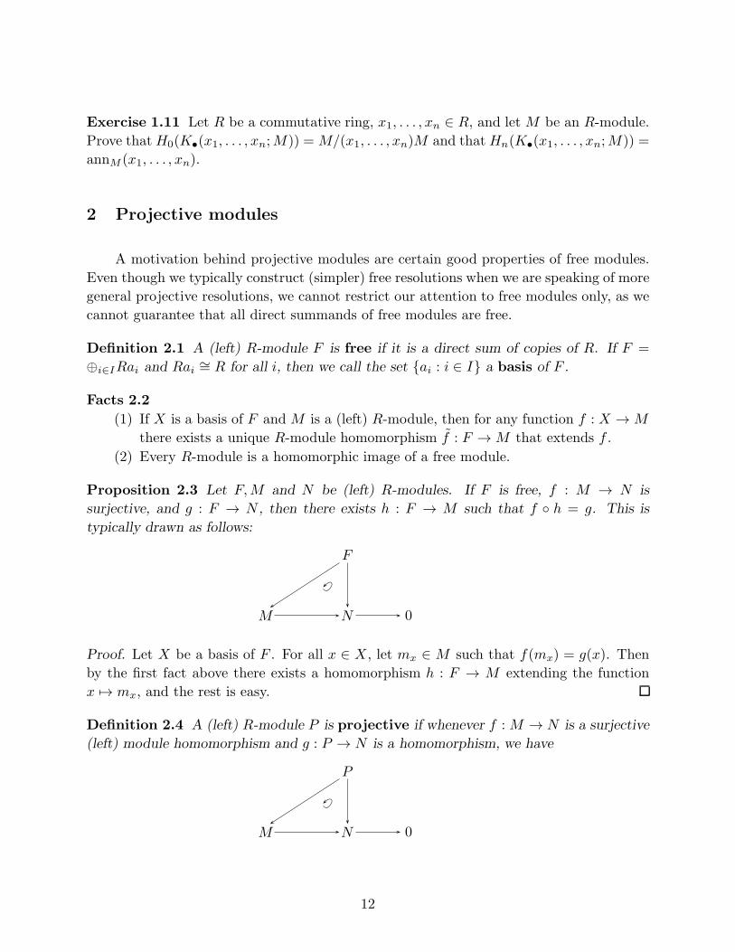
Proposition 2.3 Let F,M and N be (left) R-modules. If F is free, f : M → N is
surjective, and g : F → N , then there exists h : F → M such that f ◦ h = g. This is
typically drawn as follows:
F
M N 0
Proof. Let X be a basis of F . For all x ∈ X, let mx ∈ M such that f(mx) = g(x). Then
by the first fact above there exists a homomorphism h : F → M extending the function
x 7→ mx, and the rest is easy.
Definition 2.4 A (left) R-module P is projective if whenever f :M → N is a surjective
(left) module homomorphism and g : P → N is a homomorphism, we have
P
M N 0
12
Theorem 2.5 The following are equivalent for a left R-module P :
(1) P is projective.
(2) HomR(P, ) is exact.
(3) If Mf→→ P , then there exists h : P →M such that f ◦ h = idP .
(4) If Mf→→ P , then M ∼= P ⊕ ker f .
(5) There exists a free R-module F such that F ∼= P ⊕Q for some left R-module Q.
(Note that by the equivalences, this Q is necessarily projective.)
(6) Given a single free R-module F with Ff→→ P , there is h : P → F such that
f ◦ h = idP .
(7) Given a single free R-module F with Ff→→ P , HomR(P, F )
f◦−−→→ HomR(P, P ) is
onto.
Proof. By Exercise 1.7, HomR(P, ) is left-exact. So condition (2) is equivalent to say-
ing that HomR(P,M)◦f−−→→ HomR(P,N) is onto whenever M
f→→ N is onto. But this is
equivalent to P being projective. Thus (1) ⇔ (2).
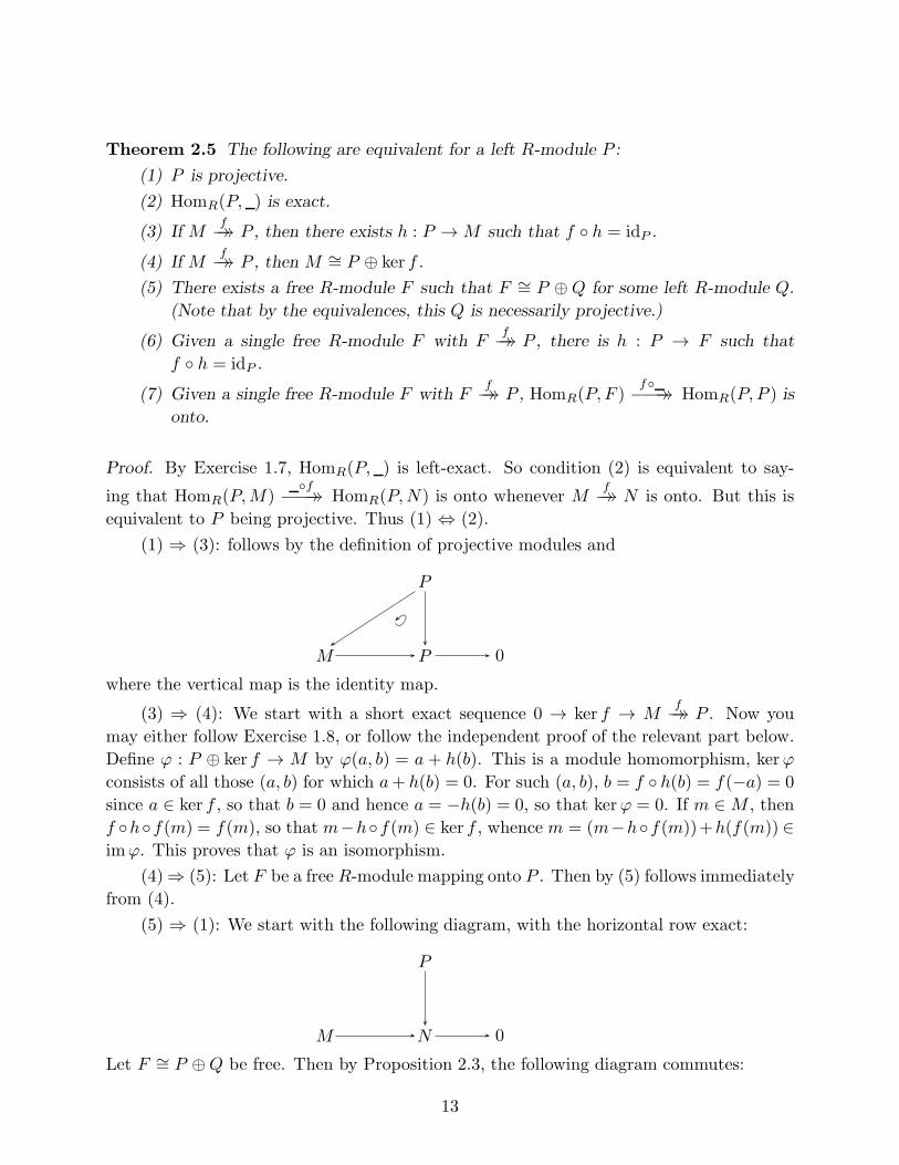
(1) ⇒ (3): follows by the definition of projective modules and
P
M P 0
where the vertical map is the identity map.
(3) ⇒ (4): We start with a short exact sequence 0 → ker f → Mf→→ P . Now you
may either follow Exercise 1.8, or follow the independent proof of the relevant part below.
Define ϕ : P ⊕ ker f → M by ϕ(a, b) = a + h(b). This is a module homomorphism, kerϕ
consists of all those (a, b) for which a+ h(b) = 0. For such (a, b), b = f ◦ h(b) = f(−a) = 0
since a ∈ ker f , so that b = 0 and hence a = −h(b) = 0, so that kerϕ = 0. If m ∈M , then
f ◦h◦f(m) = f(m), so that m−h◦f(m) ∈ ker f , whence m = (m−h◦f(m))+h(f(m)) ∈imϕ. This proves that ϕ is an isomorphism.
(4)⇒ (5): Let F be a free R-module mapping onto P . Then by (5) follows immediately
from (4).
(5) ⇒ (1): We start with the following diagram, with the horizontal row exact:
P
M N 0
Let F ∼= P ⊕Q be free. Then by Proposition 2.3, the following diagram commutes:
13
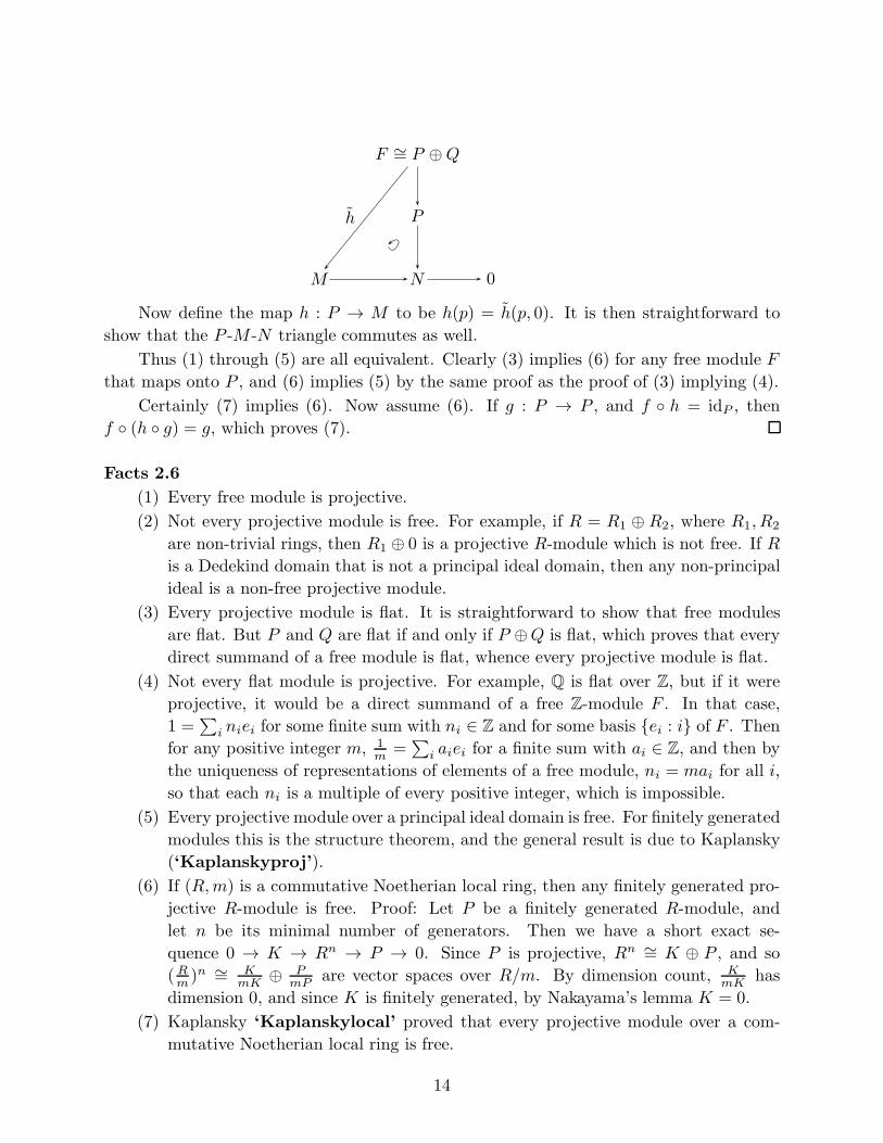
F ∼= P ⊕Q
P
M N 0
h
Now define the map h : P → M to be h(p) = h(p, 0). It is then straightforward to
show that the P -M -N triangle commutes as well.
Thus (1) through (5) are all equivalent. Clearly (3) implies (6) for any free module F
that maps onto P , and (6) implies (5) by the same proof as the proof of (3) implying (4).
Certainly (7) implies (6). Now assume (6). If g : P → P , and f ◦ h = idP , then
f ◦ (h ◦ g) = g, which proves (7).
Facts 2.6
(1) Every free module is projective.
(2) Not every projective module is free. For example, if R = R1 ⊕ R2, where R1, R2
are non-trivial rings, then R1 ⊕ 0 is a projective R-module which is not free. If R
is a Dedekind domain that is not a principal ideal domain, then any non-principal
ideal is a non-free projective module.
(3) Every projective module is flat. It is straightforward to show that free modules
are flat. But P and Q are flat if and only if P ⊕Q is flat, which proves that every
direct summand of a free module is flat, whence every projective module is flat.
(4) Not every flat module is projective. For example, Q is flat over Z, but if it were
projective, it would be a direct summand of a free Z-module F . In that case,
1 =∑
i niei for some finite sum with ni ∈ Z and for some basis {ei : i} of F . Then
for any positive integer m, 1m
=∑
i aiei for a finite sum with ai ∈ Z, and then by
the uniqueness of representations of elements of a free module, ni = mai for all i,
so that each ni is a multiple of every positive integer, which is impossible.
(5) Every projective module over a principal ideal domain is free. For finitely generated
modules this is the structure theorem, and the general result is due to Kaplansky
(‘Kaplanskyproj’).
(6) If (R,m) is a commutative Noetherian local ring, then any finitely generated pro-
jective R-module is free. Proof: Let P be a finitely generated R-module, and
let n be its minimal number of generators. Then we have a short exact se-
quence 0 → K → Rn → P → 0. Since P is projective, Rn ∼= K ⊕ P , and so
(Rm )n ∼= K
mK ⊕ PmP are vector spaces over R/m. By dimension count, K
mK has
dimension 0, and since K is finitely generated, by Nakayama’s lemma K = 0.
(7) Kaplansky ‘Kaplanskylocal’ proved that every projective module over a com-
mutative Noetherian local ring is free.
14
(8) Quillen and Suslin ‘Quillen’, ‘Suslin’ proved that every projective module over
a polynomial ring over a field is free.
Definition 2.7 Let R be a commutative ring. A vector [a1, . . . , an] ∈ Rn is unimodular
if (a1, . . . , an)R = R.
Every unimodular vector v gives rise to a projective module: Let P be the cokernel P
of the map vT : R → Rn. By Exercise 1.8, P is a direct summand of Rn, hence projective.
In fact, in this case, the P ⊕ R ∼= Rn.
Definition 2.8 An R-module P is stably free if there exist free R-modules F1 and F2
such that P ⊕ F1∼= F2.
Clearly every stably free module is projective, but the converse is not true. (Example?)
Serre proved ‘Serrestablyfree’ that every stably free module over a polynomial ring over
a field is free. We proved above that every unimodular vector gives rise to a stably free
module.
Proposition 2.9 Let R be a commutative domain. Let I be an ideal in R such that
Rm ⊕ I ∼= Rn for some m,n. Then I is free and isomorphic to Rn−m.
Proof. If I = 0, necessarily n = m, and Rn−m = 0. Now assume that I is non-zero. The
proof of this case is already worked out step by step in Exercise 1.9. For fun we give here
another proof, which is shorter but involves more machinery. By localization at R \ {0} we
know that n−m = 1. We apply ∧n.
R ∼= ∧nRn ∼= ∧n(Rn−1 ⊕ I)
∼=n∑
i=0
((∧iRn−1)⊗ (∧n−iI)) (verify)
∼= ((∧n−1Rn−1)⊗ (∧1I))⊕ ((∧nRn−1)⊗ (∧0I))
(since I has rank 1 and higher exterior powers vanish)
∼= (R⊗ I)⊕ (0⊗R) ∼= I.
Definition 2.10 An R-module P is finitely presented if it is finitely generated and the
kernel of the surjection of some finitely generated free module ontoM is finitely generated.
15
Proposition 2.11 Let R be a commutative ring and let P be a finitely presented R-
module. Then P is projective if and only if PQ is projective for all Q ∈ SpecR, and this
holds if and only if PM is projective for all M ∈ MaxR.
Proof. Let 0 → K → Rn → P → 0 be a short exact sequence with K finitely generated.
By Theorem 2.5, P is projective if and only if HomR(P,Rn) → HomR(P, P ) is onto. But
this map is onto if and only if it is onto after localization either at all prime ideals or at all
maximal ideals. But for a finitely presented module P , and for any multiplicatively closed
set W in R, W−1(HomR(P, )) ∼= HomW−1R(W−1P,W−1( )). (Verify in Exercise 2.13.)
Exercise 2.12 (Base change) Let R be a ring, S an R-algebra, and P a projective R-
module. Prove that P ⊗R S is a projective R-module.
Exercise 2.13 Let P be a finitely presented module over a commutative ring R.
Let W be a multiplicatively closed set in R. Prove that W−1(HomR(P, )) ∼=HomW−1R(W
−1P,W−1( )).
Exercise 2.14 Let r, n be positive integers and let r divide n. Prove that the (Z/nZ)-
module r(Z/nZ) is projective if and only if gcd(r, n/r) = 1. Prove that 2(Z/4Z) is not a
projective module over Z/4Z. Prove that 2(Z/6Z) is projective over Z/6Z but not free.
Exercise 2.15 Let D be a Dedekind domain. Prove that every ideal in D is a projective
D-module.
Exercise 2.16 Let R be a commutative Noetherian domain in which every ideal is a
projective R-module. Prove that R is a Dedekind domain.
Exercise 2.17 Find a Dedekind domain that is not a principal ideal domain. Give another
example of a projective module that is not free.
Exercise 2.18 If P is a finitely generated projective module over a ring R, show that
HomR(P,R) is also a projective R-module. If Q is a projective R-module, prove that
P ⊗R Q is also a projective R-module.
3 Projective, flat, free resolutions
Now that we know what free, flat, and projective modules are, the definition of free
and projective resolutions given on page 3 makes sense. It is easy to make up also the
definition of flat resolutions: in that case the relevant modules have to be flat.
16
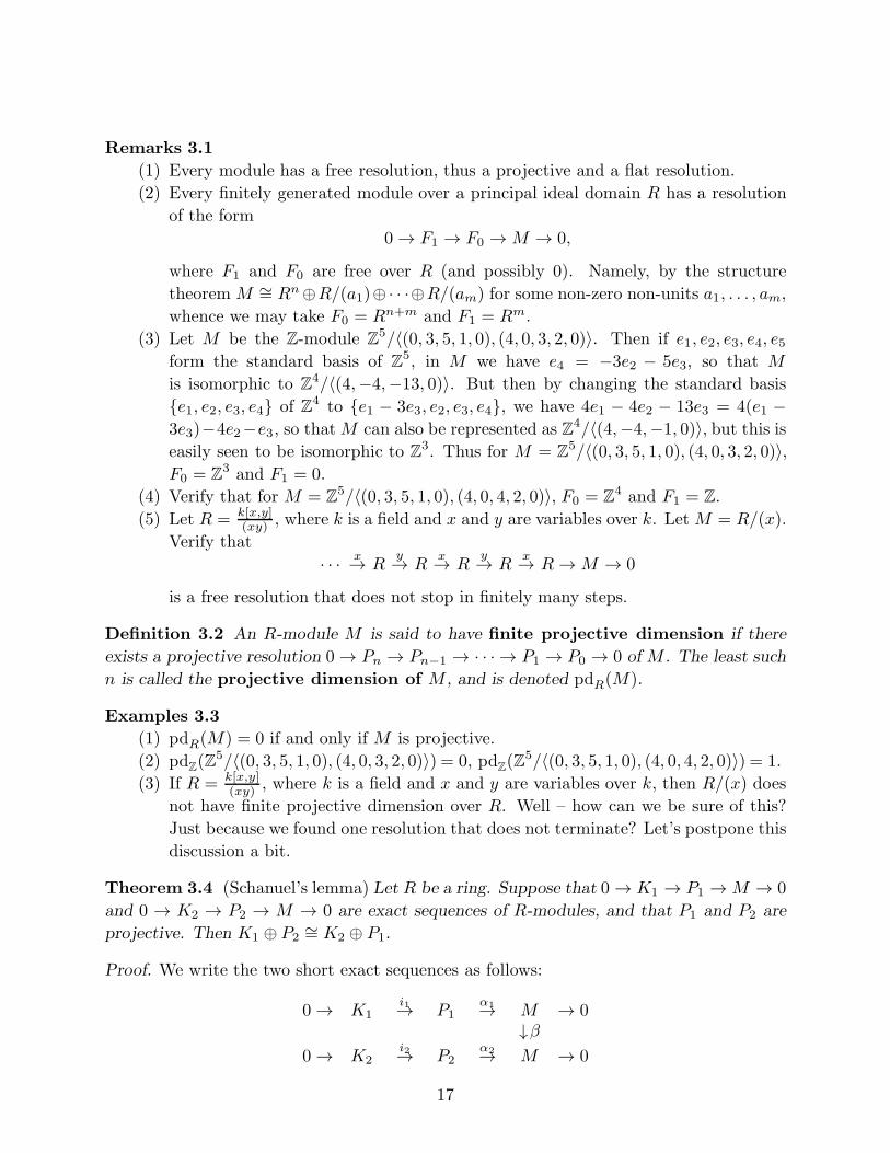
Remarks 3.1
(1) Every module has a free resolution, thus a projective and a flat resolution.
(2) Every finitely generated module over a principal ideal domain R has a resolution
of the form
0 → F1 → F0 →M → 0,
where F1 and F0 are free over R (and possibly 0). Namely, by the structure
theoremM ∼= Rn⊕R/(a1)⊕· · ·⊕R/(am) for some non-zero non-units a1, . . . , am,
whence we may take F0 = Rn+m and F1 = Rm.
(3) Let M be the Z-module Z5/〈(0, 3, 5, 1, 0), (4, 0, 3, 2, 0)〉. Then if e1, e2, e3, e4, e5form the standard basis of Z5, in M we have e4 = −3e2 − 5e3, so that M
is isomorphic to Z4/〈(4,−4,−13, 0)〉. But then by changing the standard basis
{e1, e2, e3, e4} of Z4 to {e1 − 3e3, e2, e3, e4}, we have 4e1 − 4e2 − 13e3 = 4(e1 −3e3)−4e2−e3, so thatM can also be represented as Z4/〈(4,−4,−1, 0)〉, but this iseasily seen to be isomorphic to Z3. Thus for M = Z5/〈(0, 3, 5, 1, 0), (4, 0, 3, 2, 0)〉,F0 = Z3 and F1 = 0.
(4) Verify that for M = Z5/〈(0, 3, 5, 1, 0), (4, 0, 4, 2, 0)〉, F0 = Z4 and F1 = Z.
(5) Let R = k[x,y](xy) , where k is a field and x and y are variables over k. LetM = R/(x).
Verify that
· · · x→ Ry→ R
x→ Ry→ R
x→ R→M → 0
is a free resolution that does not stop in finitely many steps.
Definition 3.2 An R-module M is said to have finite projective dimension if there
exists a projective resolution 0 → Pn → Pn−1 → · · · → P1 → P0 → 0 of M . The least such
n is called the projective dimension of M , and is denoted pdR(M).
Examples 3.3
(1) pdR(M) = 0 if and only if M is projective.
(2) pdZ(Z5/〈(0, 3, 5, 1, 0), (4, 0, 3, 2, 0)〉) = 0, pd
Z(Z5/〈(0, 3, 5, 1, 0), (4, 0, 4, 2, 0)〉) = 1.
(3) If R = k[x,y](xy)
, where k is a field and x and y are variables over k, then R/(x) does
not have finite projective dimension over R. Well – how can we be sure of this?
Just because we found one resolution that does not terminate? Let’s postpone this
discussion a bit.
Theorem 3.4 (Schanuel’s lemma) Let R be a ring. Suppose that 0 → K1 → P1 →M → 0
and 0 → K2 → P2 → M → 0 are exact sequences of R-modules, and that P1 and P2 are
projective. Then K1 ⊕ P2∼= K2 ⊕ P1.
Proof. We write the two short exact sequences as follows:
0 → K1i1→ P1
α1→ M → 0↓β
0 → K2i2→ P2
α2→ M → 0
17
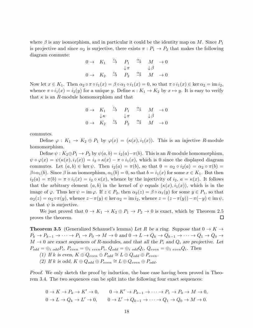
where β is any isomorphism, and in particular it could be the identity map onM . Since P1
is projective and since α2 is surjective, there exists π : P1 → P2 that makes the following
diagram commute:
0 → K1i1→ P1
α1→ M → 0↓π ↓β
0 → K2i2→ P2
α2→ M → 0
Now let x ∈ K1. Then α2 ◦ π ◦ i1(x) = β ◦α1 ◦ i1(x) = 0, so that π ◦ i1(x) ∈ kerα2 = im i2,
whence π ◦ i1(x) = i2(y) for a unique y. Define κ : K1 → K2 by x 7→ y. It is easy to verify
that κ is an R-module homomorphism and that
0 → K1i1→ P1
α1→ M → 0↓κ ↓π ↓β
0 → K2i2→ P2
α2→ M → 0
commutes.
Define ϕ : K1 → K2 ⊕ P1 by ϕ(x) = (κ(x), i1(x)). This is an injective R-module
homomorphism.
Define ψ : K2⊕P1 → P2 by ψ(a, b) = i2(a)−π(b). This is anR-module homomorphism,
ψ ◦ ϕ(x) = ψ(κ(x), i1(x)) = i2 ◦ κ(x) − π ◦ i1(x), which is 0 since the displayed diagram
commutes. Let (a, b) ∈ kerψ. Then i2(a) = π(b), so that 0 = α2 ◦ i2(a) = α2 ◦ π(b) =
β◦α1(b). Since β is an isomorphism, α1(b) = 0, so that b = i1(x) for some x ∈ K1. But then
i2(a) = π(b) = π ◦ i1(x) = i2 ◦ κ(x), whence by the injectivity of i2, a = κ(x). It follows
that the arbitrary element (a, b) in the kernel of ψ equals (κ(x), i1(x)), which is in the
image of ϕ. Thus kerψ = imϕ. If z ∈ P2, then α2(z) = β ◦ α1(y) for some y ∈ P1, so that
α2(z) = α2 ◦π(y), whence z−π(y) ∈ kerα2 = im i2, whence z = (z−π(y))−π(−y) ∈ imψ,
so that ψ is surjective.
We just proved that 0 → K1 → K2 ⊕ P1 → P2 → 0 is exact, which by Theorem 2.5
proves the theorem.
Theorem 3.5 (Generalized Schanuel’s lemma) Let R be a ring. Suppose that 0 → K →Pk → Pk−1 → · · · → P1 → P0 → M → 0 and 0 → L → Qk → Qk−1 → · · · → Q1 → Q0 →M → 0 are exact sequences of R-modules, and that all the Pi and Qi are projective. Let
Podd = ⊕i oddPi, Peven = ⊕i evenPi, Qodd = ⊕i oddQi, Qeven = ⊕i evenQi. Then
(1) If k is even, K ⊕Qeven ⊕ Podd∼= L⊕Qodd ⊕ Peven.
(2) If k is odd, K ⊕Qodd ⊕ Peven∼= L⊕Qeven ⊕ Podd.
Proof. We only sketch the proof by induction, the base case having been proved in Theo-
rem 3.4. The two sequences can be split into the following four exact sequences:
0 → K → Pk → K′ → 0, 0 → K′ → Pk−1 → · · · → P1 → P0 →M → 0,
0 → L→ Qk → L′ → 0, 0 → L′ → Qk−1 → · · · → Q1 → Q0 →M → 0.
18
By induction, K′ direct sum with some projective module A is isomorphic to L′ direct sumwith some projective module B. Then the two short exact sequences above yield the short
exact sequences below:
0 → K → Pk ⊕A→ K′ ⊕A→ 0,
0 → L→ Qk ⊕B → L′ ⊕B → 0.
Then by the first version of Schanuel’s lemma Theorem 3.4, at least by the proof in which
we allow the extreme right modules to not necessarily be identical but only isomorphic,
K ⊕Qk ⊕B ∼= L⊕Pk ⊕A. Now it remains to prove that the forms for odd and even k are
as given.
Theorem 3.6 (Minimal resolutions over Noetherian local rings) Let (R,m) be a Noethe-
rian local ring, and let M be a finitely generated R-module with finite projective dimen-
sion n. Define b0 = µ(M), so that we have a part of a free resolution of M over R:
Rb0 → M → 0. Then recursively, after b0, . . . , bi have been defined and Rbi → Rbi−1 →· · · → Rb1 → Rb0 → M → 0 is exact, let bi+1 be the number of generators of the kernel
of Rbi → Rbi−1 , so that we can extend the beginning of the resolution by one step. Then
bn 6= 0 and bn+1 = 0. In other words, a projective resolution of minimal length may be ob-
tained by constructing a free resolution in which at each step we take the minimal possible
number of generators of the free modules.
Proof. By assumption there exists a projective resolution 0 → Pn → Pn−1 → · · · → P1 →P0 → M → 0. Let K be the kernel of Rbn → Rbn−1 in our construction. Then by the
generalized Schanuel’s lemma Theorem 3.5, the direct sum of K and some projective R-
module is isomorphic to another projective R-module, whence it follows quickly from the
definitions of projective modules that K is also projective. Since K is a submodule of a
finitely generated R-module and R is Noetherian, K is also finitely generated, so that by
Facts 2.6 (6), K is free. This means that our minimal resolution construction is at most as
long as the minimal projective resolution, and so by minimality bn 6= 0 and bn+1 = 0.
Exercise 3.7 Let R be a polynomial ring in finitely many variables over a field. Let M
be a graded finitely generated R-module. We will prove later (see Theorem 8.6) initely
generated R-module has finite projective dimension. Let n be the projective dimension
of M . Let · · · → Rbi → Rbi−1 → · · · → Rb1 → Rb0 → M → 0 be exact, with all
maps homogeneous, and with b0 chosen smallest possible, after which b1 is chosen smallest
possible, etc. Prove that all the entries of the matrices of the maps Rbi → Rbi−1 have
positive degree and may be chosen to be homogeneous. Prove that bn+1 = 0 and bn 6= 0.
Exercise 3.8 Prove that pdR(M1 ⊕M2) = sup {pdR(M1), pdR(M2)}.
19
Exercise 3.9 Let R be either a Noetherian local ring or a polynomial ring over a field. Let
M be a finitely generated R-module that is graded in case R is a polynomial ring. Let F•be a free resolution of M , and let G• be a minimal free resolution of M . Prove that there
exists an exact complex H• such that F• ∼= G• ⊕H• (isomorphism of maps of complexes).
In particular, if G• is minimal, this proves that F• ∼= G•.
4 General manipulations of complexes
We need to develop more general tools that will be applicable to projective and free
resolutions, and also to injective resolutions and other complexes.
Let C• = · · ·Cn+1dn+1→ Cn
dn→ Cn−1 → · · · be a complex. We introduce the com-
mon terminology that the elements of ker dn are called the nth cycles, and that the
elements of im dn+1 are also referred to as the nth boundaries. For this reason we alsotry to
avoid
mul-
tiple
words
sometimes write Bn = imdn+1, Zn = ker dn. These are simply names that do not change
anything, and I try not to use too many words when one will do, but the following point
of view can be useful, and often notationally shorter: the complex C• can be thought of as
a differential module (⊕nCn, d•), where d• : ⊕nCn → ⊕nCn, with d•|Cn= dn, is called
the differential and has degree −1 as the image of Cn under d• is in Cn−1. The word
differential also connotes that d•2 = 0, which is on the complex side the same thing as
saying that C• is a complex. Another example of a differential module is (⊕nHn(C•), 0).
Definition 4.1 A map of complexes is a function f• : C• → C•′, where (C•, d) and
(C•′, d′) are complexes, where f• restricted to Cn is denoted fn, where fn maps to C ′n, and
such that for all n, d′n ◦ fn = fn−1 ◦ dn. In the differential graded modules terminology,
this says that f• has degree 0, and we can also write this as d′ ◦ f• = f• ◦ d. We can also
draw this as a commutative diagram:
· · · → Cn+1dn+1→ Cn
dn→ Cn−1 → · · ·↓fn+1 ↓fn ↓fn−1
· · · → C ′n+1
dn+1→ C ′ndn→ C ′n−1 → · · ·
It is clear that the kernel and the image of a map of complexes are naturally complexes.
Thus we can even talk about exact complexes of complexes, and in particular about
short exact sequences of complexes, and the following is straightforward:
Definition 4.2 Let f• : C• → C•′ be a map of complexes. Then we get the induced map
f∗ : H(C•) → H(C•′) of complexes.
An example of a short exact sequence of complexes is constructed in Proposition 5.1
in the next section, and in Proposition 6.5 later on, etc.
20
Lemma 4.3 Let 0 → C•′ → C• → C•
′′ → 0 be a short exact sequence of complexes. If all
modules in C•′ and C•
′′ are projective, so are all the modules in C•.
Proof. Since C ′′n is projective, we know that Cn ⊕ C ′n ⊕ C ′′n . Since both C ′n and C ′′n are
projective, so is Cn.
Theorem 4.4 (Short exact sequence of complexes yields a long exact sequence on homol-
ogy) Let 0 → C•′ f•−→ C
g•−→ C ′′ → 0 be a short exact sequence of complexes. Then we
have a long exact sequence on homology:
· · · → Hn+1(C•′′)
∆n+1−−−→ Hn(C•′)
f→ Hn(C•)g→ Hn(C•
′′)∆n−→ Hn−1(C•
′)f→ Hn−1(C•) → · · ·
where the arrows denoted by f and g are only induced by f and g, and the ∆ maps are
the connecting homomorphisms as in Lemma 1.5.
Proof. By assumption we have the following commutative diagram with exact rows:
0 → C ′nfn→ Cn
gn→ C ′′n → 0↓d′n ↓dn ↓d′′n
0 → C ′n−1fn−1−→ Cn−1
gn−1−→ C ′′n−1 → 0.
By the Snake Lemma Lemma 1.5, we get the following exact sequences for all n:
0 → ker d′nfn−→ ker dn
gn−→ ker d′′n,
coker d′nfn−→ coker dn
gn−→ coker d′′n → 0,
where the actual maps are only those naturally induced by the marked maps. We even
have the following commutative diagram with exact rows:
coker d′nfn−→ coker dn
gn−→ coker d′′n → 0↓d′n ↓dn ↓d′′n
0 → ker d′n−1fn−1−→ ker dn−1
gn−1−→ ker d′′n−1.
Now another application of Lemma 1.5 yields exactly the desired sequence.
The following is now immediate:
Corollary 4.5 Let 0 → C•′ → C• → C•
′′ → 0 be a short exact sequence of complexes. If
C•′ and C•
′′ have zero homology, so does C•.
Definition 4.6 A map f• : C• → C•′ (of degree 0) of complexes is null-homotopic if
there exist maps sn : Cn → C ′n+1 such that for all n, fn = d′n+1 ◦ sn + sn−1 ◦ dn. Maps
f•, g• : C• → C•′ are homotopic if f• − g• is null-homotopic.
21
Proposition 4.7 If f• and g• are homotopic, then f∗ = g∗ (recall Definition 4.2).
Proof. By assumption there exist maps sn : Cn → C ′n+1 such that for all n, fn − gn =
d′n+1 ◦ sn + sn−1 ◦ dn. If z ∈ ker dn, then fn(z)− gn(z) = d′n+1 ◦ sn(z) is zero in Hn(C•′).
The following is straightforward from the definitions (and no proof is provided here):
Proposition 4.8 If f• and g• are homotopic, so are
(1) f• ⊗ idM and g• ⊗ idM ;
(2) HomR(M, f•) and HomR(M, g•);(3) HomR(f•,M) and HomR(g•,M);
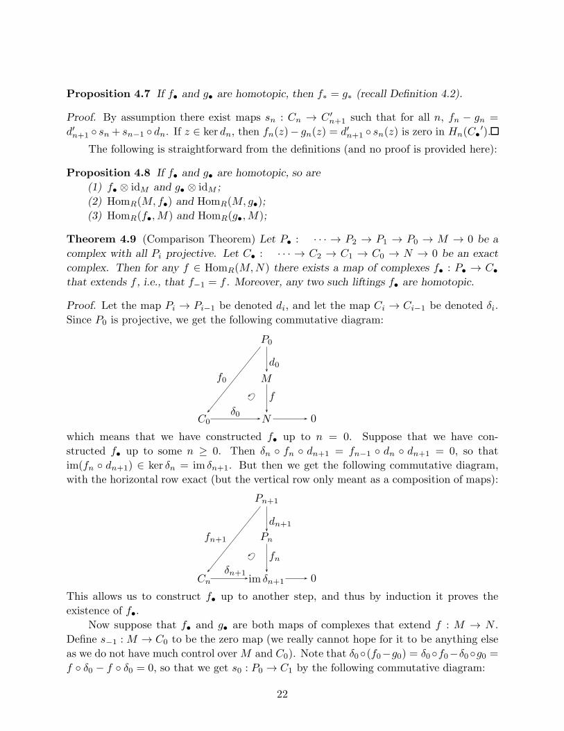
Theorem 4.9 (Comparison Theorem) Let P• : · · · → P2 → P1 → P0 → M → 0 be a
complex with all Pi projective. Let C• : · · · → C2 → C1 → C0 → N → 0 be an exact
complex. Then for any f ∈ HomR(M,N) there exists a map of complexes f• : P• → C•that extends f , i.e., that f−1 = f . Moreover, any two such liftings f• are homotopic.
Proof. Let the map Pi → Pi−1 be denoted di, and let the map Ci → Ci−1 be denoted δi.
Since P0 is projective, we get the following commutative diagram:
P0
M
C0 N 0
f0
d0
f
δ0
which means that we have constructed f• up to n = 0. Suppose that we have con-
structed f• up to some n ≥ 0. Then δn ◦ fn ◦ dn+1 = fn−1 ◦ dn ◦ dn+1 = 0, so that
im(fn ◦ dn+1) ∈ ker δn = im δn+1. But then we get the following commutative diagram,
with the horizontal row exact (but the vertical row only meant as a composition of maps):
Pn+1
Pn
Cn im δn+1 0
fn+1
dn+1
fnδn+1
This allows us to construct f• up to another step, and thus by induction it proves the
existence of f•.Now suppose that f• and g• are both maps of complexes that extend f : M → N .
Define s−1 :M → C0 to be the zero map (we really cannot hope for it to be anything else
as we do not have much control overM and C0). Note that δ0◦(f0−g0) = δ0◦f0−δ0◦g0 =
f ◦ δ0 − f ◦ δ0 = 0, so that we get s0 : P0 → C1 by the following commutative diagram:
22
P0
C1 im δ1 0
s0f0 − g0
δ1
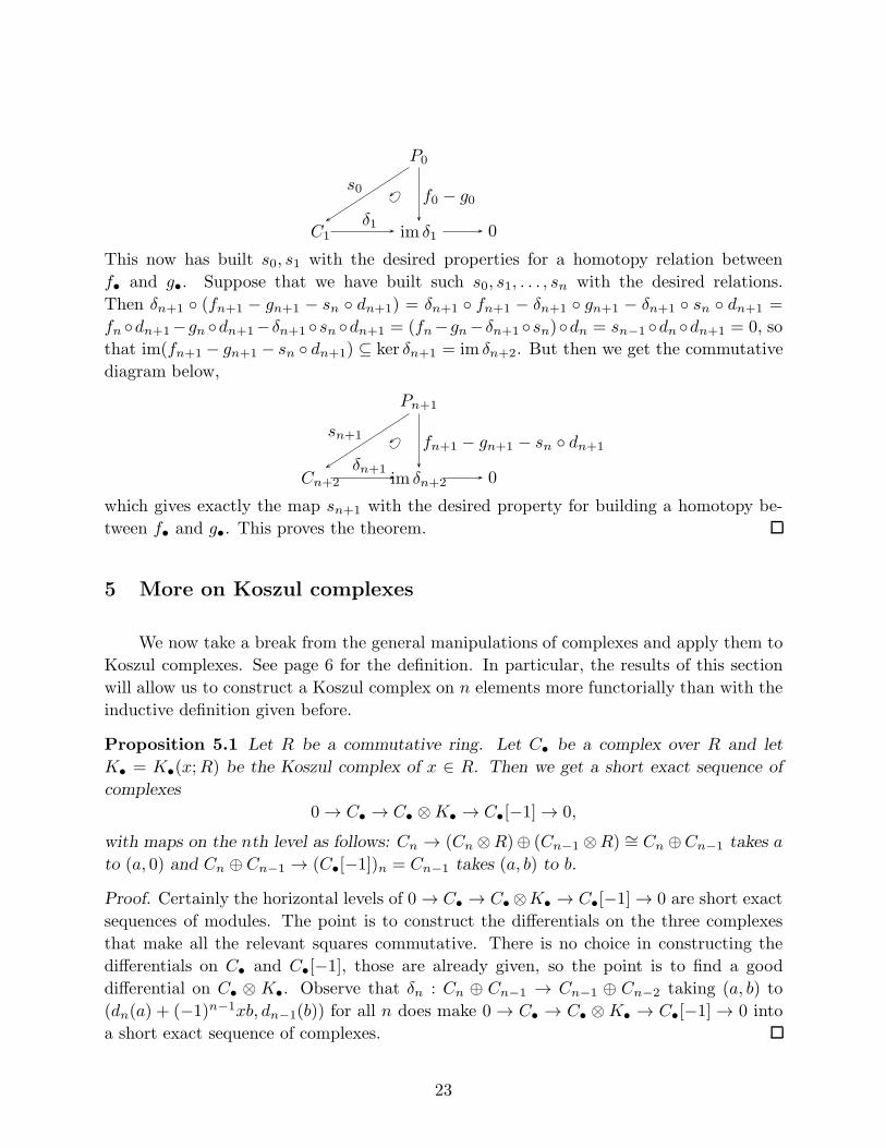
This now has built s0, s1 with the desired properties for a homotopy relation between
f• and g•. Suppose that we have built such s0, s1, . . . , sn with the desired relations.
Then δn+1 ◦ (fn+1 − gn+1 − sn ◦ dn+1) = δn+1 ◦ fn+1 − δn+1 ◦ gn+1 − δn+1 ◦ sn ◦ dn+1 =
fn ◦dn+1−gn ◦dn+1−δn+1 ◦sn ◦dn+1 = (fn−gn−δn+1 ◦sn)◦dn = sn−1 ◦dn ◦dn+1 = 0, so
that im(fn+1 − gn+1 − sn ◦ dn+1) ⊆ ker δn+1 = im δn+2. But then we get the commutative
diagram below,
Pn+1
Cn+2 im δn+2 0
sn+1 fn+1 − gn+1 − sn ◦ dn+1
δn+1
which gives exactly the map sn+1 with the desired property for building a homotopy be-
tween f• and g•. This proves the theorem.
5 More on Koszul complexes
We now take a break from the general manipulations of complexes and apply them to
Koszul complexes. See page 6 for the definition. In particular, the results of this section
will allow us to construct a Koszul complex on n elements more functorially than with the
inductive definition given before.
Proposition 5.1 Let R be a commutative ring. Let C• be a complex over R and let
K• = K•(x;R) be the Koszul complex of x ∈ R. Then we get a short exact sequence of
complexes
0 → C• → C• ⊗K• → C•[−1] → 0,
with maps on the nth level as follows: Cn → (Cn ⊗R)⊕ (Cn−1 ⊗R) ∼= Cn ⊕Cn−1 takes a
to (a, 0) and Cn ⊕ Cn−1 → (C•[−1])n = Cn−1 takes (a, b) to b.
Proof. Certainly the horizontal levels of 0 → C• → C•⊗K• → C•[−1] → 0 are short exact
sequences of modules. The point is to construct the differentials on the three complexes
that make all the relevant squares commutative. There is no choice in constructing the
differentials on C• and C•[−1], those are already given, so the point is to find a good
differential on C• ⊗ K•. Observe that δn : Cn ⊕ Cn−1 → Cn−1 ⊕ Cn−2 taking (a, b) to
(dn(a) + (−1)n−1xb, dn−1(b)) for all n does make 0 → C• → C• ⊗K• → C•[−1] → 0 into
a short exact sequence of complexes.
23
Corollary 5.2 With hypotheses as above, we get a long exact sequence
· · · x→ Hn(C•) → Hn(C• ⊗K•) → Hn−1(C•)x→ Hn−1(C•) → Hn−1(C• ⊗K•) → · · ·
Proof. First of all, Hn−1(C•) = Hn(C•[−1]), so that the long exact sequence above is a
consequence of the previous proposition and of Theorem 4.4. Furthermore, we need to go
through the proof of the previous proposition, of Theorem 4.4, and of the Snake Lemma
Lemma 1.5, to verify that the connecting homomorphisms are indeed just multiplications
by x.
The long exact sequence in the corollary breaks into short exact sequences:
0 → Hn(C•)
xHn(C•)→ Hn(C• ⊗K•) → annHn−1(C•)(x) → 0 (5.3)
for all n, where annM (N) denotes the set of all elements of M that annihilate N .
Definition 5.4 We say that x1, . . . , xn ∈ R is a regular sequence on a module M , or
a M-regular sequence if (x1, . . . , xn)M 6= M and if for all i = 1, . . . , n, xi is a non-
zerodivisor on M/(x1, . . . , xi−1)M . We say that x1, . . . , xn ∈ R is a regular sequence if
it is a regular sequence on the R-module R.
Corollary 5.5 Let x1, . . . , xn be a regular sequence on a commutative ring R. Then
Hi(K•(x1, . . . , xn;R)) =
{0 if i > 0;
R(x1,...,xn)
if i = 0.
Thus K•(x1, . . . , xn;R) is a free resolution of R(x1,...,xn)
.
Proof. This is trivially verified if n = 1. Now let n > 1. Let C• = K•(x1, . . . , xn−1;R),K• = K•(xn;R). By the short exact sequences above, by induction on n,Hi(K•(x1, . . . , xn;R)) =Hi(C• ⊗K•) = 0 if i > 1 (as Hi(C•) and Hi−1(C•) are both 0). If i = 1, we get
0 → 0 =H1(C•)
xnH1(C•)→ H1(C• ⊗K•) → annH0(C•)(xn) → 0,
so that H1(C• ⊗ K•) ∼= annH0(C•)(xn), and by induction this is annR/(x1,...,xn−1)(xn).
Since xn is a non-zerodivisor on R/(x1, . . . , xn−1), we get that H1(K•(x1, . . . , xn;R)) =
H1(C•⊗K•) = 0. Finally, for i = 0, the short exact sequence gives H0(C•)xnH0(C•)
∼= H0(C•⊗K•),and again by induction on n this says that H0(K•(x1, . . . , xn;R)) = H0(C• ⊗ K•) ∼=H0(C•)xH0(C•)
∼= R/(x1, . . . , xn).
Exercise 5.6 (Depth sensitivity of Koszul complexes) Let R be a commutative ring
and M an R-module. Let x1, . . . , xn ∈ R. Assume that x1, . . . , xl is a regular sequence on
M for some l ≤ n. Prove that Hi(K•(x1, . . . , xn;M)) = 0 for i = n, n− 1, . . . , n− l + 1.
24
Exercise 5.7 Let R be a commutative ring, x1, . . . , xn ∈ R, and M an R-module. Prove
that (x1, . . . , xn) annihilates each Hn(K•(x1, . . . , xn;M)).
Exercise 5.8 Let I = (x1, . . . , xn) = (y1, . . . , ym) be an ideal contained in the Ja-
cobson radical of a commutative ring R. Let M be a finitely generated R-module.
Suppose that Hi(K•(x1, . . . , xn;M)) = 0 for i = n, n − 1, . . . , n − l + 1. Prove that
Hi(K•(y1, . . . , ym;M)) = 0 for i = m,m− 1, . . . , m− l + 1.
6 General manipulations applied to projective resolutions
Proposition 6.1 Let P• be a projective resolution of M , let Q• be a projective resolution
of N , and let f ∈ HomR(M,N). Then there exists a map of complexes f• : P• → Q• suchthat
P• → M → 0↓f• ↓fQ• → N → 0
commutes. Furthermore, any two such f• are homotopic.
Proof. This is just an application of the Comparison Theorem Theorem 4.9.
Corollary 6.2 Let P• and Q• be projective resolutions of M . Then there exists a map of
complexes f• : P• → Q• such that
P• → M → 0↓f• ↓ idMQ• → N → 0
commutes. Furthermore, any two such f• are homotopic.
Corollary 6.3 Let P• and Q• be projective resolutions of M . Then for any additive
functor F, the homologies of F(P•) and of F(Q•) are isomorphic.
Proof. By Corollary 6.2 there exists f• : P• → Q• that extends idM , and there exists
g• : Q• → P• that extends idM . Thus f• ◦ g• : Q• → Q• extends idM , but so does
the identity map on Q•. Thus by the Comparison Theorem Theorem 4.9, f• ◦ g• and id
are homotopic, whence so are F(f• ◦ g•) and F(id). Thus by Proposition 4.7, the map
(F(f• ◦ g•))∗ induced on the homology of F(Q•) is the identity map. If F is covariant,
this says that (F(f•))∗ ◦ (F(g•))∗ is identity, whence (F(f•))∗ is surjective and (F(g•))∗ isinjective. Similarly, by looking at the other composition, we get that (F(g•))∗ is surjectiveand (F(f•))∗ is injective. Thus (F(f•))∗ is an isomorphism, which proves the corollary in
case F is covariant. The argument for contravariant functors is similar.
25
Lemma 6.4 Suppose that
0 → C•′ → C• → C•
′′ → 0↓ ↓ ↓
0 → M ′ → M → M ′′ → 0
is a commutative diagram, in which the bottom row is a short exact sequence of modules
and the top row is a short exact sequence of complexes. If C•′ is a projective resolution of
M ′ and C•′′ is a projective resolution of M ′′, then C• is a projective resolution of M .
Proof. By Corollary 4.5 we know that C• → M → 0 has no homology, and by Lemma 4.3
we know that all the modules in C• are projective. This proves the lemma.
Proposition 6.5 Let C•′ be a projective resolution of M ′ and let C•
′′ be a projective
resolution of M ′′. Suppose that 0 →M ′ →M →M ′′ → 0 is a short exact sequence. Then
there exists a projective resolution C• such that
0 → C•′ → C• → C•
′′ → 0↓ ↓ ↓
0 → M ′ → M → M ′′ → 0
is a commutative diagram, in which the top row is a short exact sequence of complexes.
Proof. Define Cn = C ′n ⊕ C ′′n , giving the modules of C•, with the horizontal maps in the
short exact sequence 0 → C ′nin→ Cn
πn→ C ′′n → 0 the obvious maps. We have to work harder
to construct the differential maps on C•.Consider the following set-up with exact rows:
· · · → C ′′2 → C ′′1 → C ′′0 → M ′′ → 0||
· · · → C ′1 → C ′0 → M → M ′′ → 0
By the Comparison Theorem (Theorem 4.9), there exist maps t0 : C ′′0 →M and tn : C ′′n →C ′n−1 for n ≥ 1 that make the filled-in displayed diagram above commute.
Now define d0 : C0 → M as d0(a, b) = i ◦ d′0(a) + t0(b), and dn : Cn → Cn−1 as
dn(a, b) = (d′n(a) + (−1)ntn(b), d′′n(b)) for n ≥ 1. The reader should verify the rest.
Exercise 6.6 Let 0 → M ′ → M → M ′′ → 0 be a short exact sequence of R-modules.
Prove that pdR(M) ≤ sup {pdR(M ′), pdR(M ′′)}. If pdR(M) < sup {pdR(M ′), pdR(M ′′)},prove that pdR(M
′′) = pdR(M′) + 1.
Exercise 6.7 Let 0 → M ′ → M → M ′′ → 0 be a short exact sequence of R-modules.
Prove that if any two of the modules have finite projective dimension, so does the third.
26
Exercise 6.8 Let R be a commutative ring. Let 0 → Mn → Pn−1 → · · · → P1 →P0 → M → 0 be an exact sequence of R-modules, where all Pi are projective. Prove
that pdR(M) ≤ n if and only if Mn is projective. Prove that if pdR(M) ≥ n, then
pdR(M) = pd(Mn)− n.
Exercise 6.9 Let R be a Noetherian ring and M a finitely generated R-module Prove
that pdR(M) = sup {pdRp(Mp) : p ∈ SpecR}.
7 Tor
Let M,N be R-modules, and let P• : · · ·P2 → P1 → P0 → 0 be a projective
resolution of M . We define
TorRn (M,N) = Hn(P• ⊗R N).
With all the general manipulations of complexes we can fairly quickly develop some
main properties of Tor:
1. Independence of the resolution. The definition of TorRn (M, ) is independent of the
projective resolution P• of M . This follows from Corollary 6.3.
2. Tor has no terms of negative degree. TorRn (M, ) = 0 if n < 0. This follows as P•has only zero modules in negative positions.
3. Tor0. TorR0 (M,N) ∼=M ⊗RN . Proof: By assumption P1 → P0 →M → 0 is exact, and
as ⊗R N is right-exact, P1 ⊗R N → P0 ⊗R N → M ⊗R N → 0 is exact as well. Thus
TorR0 (M,N) = H0(P• ⊗R N) = (P0 ⊗R N)/ im(P1 ⊗R N) ∼=M ⊗R N .
4. What if M is projective? If M is projective, then TorRn (M,N) = 0 for all n ≥ 1.
This is clear as in that case we may take P0 =M and all other Pn to be 0.
5. What if N is flat? If N is flat, then TorRn (M,N) = 0 for all n ≥ 1. This follows as
Pn+1 → Pn → Pn−1 is exact, and so as N is flat, Pn+1 ⊗ N → Pn ⊗ N → Pn−1 ⊗ N is
exact as well, giving that the nth homology of P• ⊗N is 0 if n > 0.
6. Tor on short exact sequences. If 0 → M ′ → M → M ′′ → 0 is a short exact se-
quence of modules, then for any module N , there is a long exact sequence
· · · → TorRn+1(M′′, N) → TorRn (M
′, N) → TorRn (M,N) → TorRn (M′′, N) → TorRn−1(M
′, N) → · · · .
The proof goes as follows. Let P•′ be a projective resolution of M ′, and let P•
′′ be a
projective resolution of M ′′. Then by Proposition 6.5 there exists a projective resolution
P• of M such that0 → P•
′ → P• → P•′′ → 0
↓ ↓ ↓0 → M ′ → M → M ′′ → 0
27
is a commutative diagram in which the rows are exact. In particular, we have a short exact
sequence 0 → P•′ → P• → P•
′′ → 0, and since this is a split exact sequence, it follows that
0 → P•′ ⊗N → P• ⊗N → P•
′′ ⊗N → 0 is still a short exact sequence of complexes. The
rest follows from Theorem 4.4.
7. Tor and annihilators. For any M,N and n, annM + annN ⊆ ann TorRn (M,N).
Proof: Since TorRn (M,N) is a quotient of a submodule of Pn × N , it is clear that annN
annihilates all Tors. Now let x ∈ annM . Then multiplication by x on M , which is the
same as multiplication by 0 on M , has two lifts µx and µ0 on P•, and by the Comparison
Theorem Theorem 4.9, the two maps are homotopic. Thus µx ⊗ idN and 0 are homotopic
on P• × N , whence by Proposition 4.7, (µx ⊗ idN )∗ = 0. But (µx ⊗ idN )∗ is simply
multiplication by x, which says that multiplication by x on TorRn (M,N) is 0. This proves
that indeed annM + annN ⊆ ann TorRn (M,N).
8. Tor on syzygies. Let 0 → Mn → Pn−1 → · · · → P1 → P0 → M → 0 be an exact
sequence (with Pi part of the projective resolution P• of M). Such Mn is called an nth
syzygy of M . Then for all i ≥ 1, TorRi (Mn, N) ∼= TorRi+n(M,N). This follows from the
definition of Tor (and from the independence on the projective resolution).
9. Tor for finitely generated modules over Noetherian rings. If R is Noetherian
and M and N are finitely generated R-modules, then TorRn (M,N) is a finitely generated
R-module for all n. To prove this, we may choose P• such that all Pn are finitely generated
(since submodules of finitely generated modules are finitely generated). Then Pn ⊗ N is
finitely generated, whence so is TorRn (M,N).
Note that we do not quite have symmetric results for M and N in TorRn (M,N).
Theorem 7.1 Let R be a commutative ring and let M and N be R-modules. Then for
all n, TorRn (M,N) ∼= TorRn (N,M).
Proof. Let P• be a projective resolution of M and let Q• be a projective resolution of
N . We temporarily introduce another construction: TorR
n (M,N) = Hn(M ⊗R Q•). The
goal is to actually prove that TorRn (M,N) ∼= TorR
n (M,N) (for which we do not need a
commutative ring).
It is clear that the properties 1.–9. listed above hold in the symmetric version for Tor.
In particular, it follows that TorRn (M,N) ∼= TorR
n (M,N) for all n ≤ 0.
Let M1, N1 be defined so that 0 → M1 → P0 → M → 0 and 0 → N1 → Q0 → N → 0
28
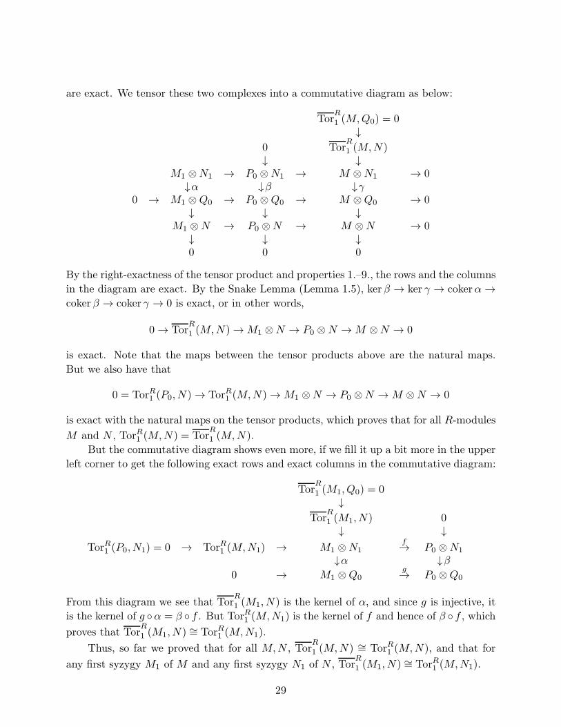
are exact. We tensor these two complexes into a commutative diagram as below:
TorR
1 (M,Q0) = 0↓
0 TorR
1 (M,N)↓ ↓
M1 ⊗N1 → P0 ⊗N1 → M ⊗N1 → 0↓α ↓β ↓γ
0 → M1 ⊗Q0 → P0 ⊗Q0 → M ⊗Q0 → 0↓ ↓ ↓
M1 ⊗N → P0 ⊗N → M ⊗N → 0↓ ↓ ↓0 0 0
By the right-exactness of the tensor product and properties 1.–9., the rows and the columns
in the diagram are exact. By the Snake Lemma (Lemma 1.5), ker β → ker γ → cokerα →coker β → coker γ → 0 is exact, or in other words,
0 → TorR
1 (M,N) →M1 ⊗N → P0 ⊗N →M ⊗N → 0
is exact. Note that the maps between the tensor products above are the natural maps.
But we also have that
0 = TorR1 (P0, N) → TorR1 (M,N) →M1 ⊗N → P0 ⊗N →M ⊗N → 0
is exact with the natural maps on the tensor products, which proves that for all R-modules
M and N , TorR1 (M,N) = TorR
1 (M,N).
But the commutative diagram shows even more, if we fill it up a bit more in the upper
left corner to get the following exact rows and exact columns in the commutative diagram:
TorR
1 (M1, Q0) = 0↓
TorR
1 (M1, N) 0↓ ↓
TorR1 (P0, N1) = 0 → TorR1 (M,N1) → M1 ⊗N1f→ P0 ⊗N1
↓α ↓β0 → M1 ⊗Q0
g→ P0 ⊗Q0
From this diagram we see that TorR
1 (M1, N) is the kernel of α, and since g is injective, it
is the kernel of g ◦α = β ◦ f . But TorR1 (M,N1) is the kernel of f and hence of β ◦ f , whichproves that Tor
R
1 (M1, N) ∼= TorR1 (M,N1).
Thus, so far we proved that for all M,N , TorR
1 (M,N) ∼= TorR1 (M,N), and that for
any first syzygy M1 of M and any first syzygy N1 of N , TorR
1 (M1, N) ∼= TorR1 (M,N1).
29
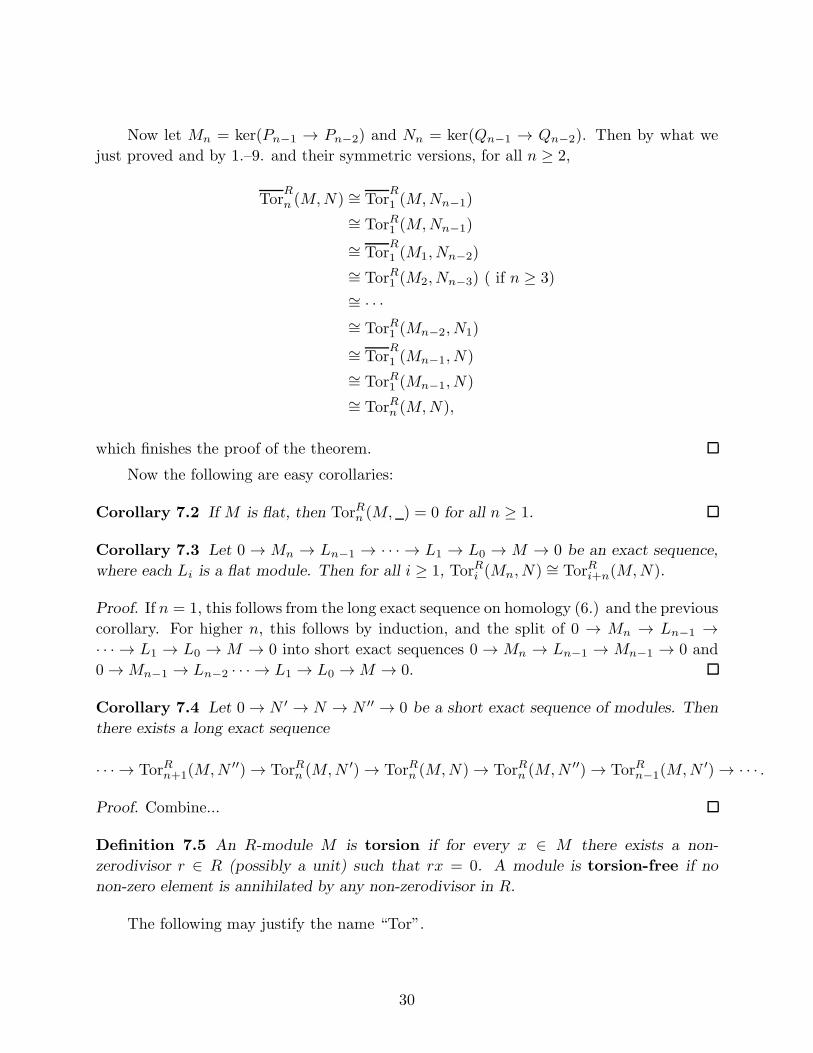
Now let Mn = ker(Pn−1 → Pn−2) and Nn = ker(Qn−1 → Qn−2). Then by what we
just proved and by 1.–9. and their symmetric versions, for all n ≥ 2,
TorR
n (M,N) ∼= TorR
1 (M,Nn−1)
∼= TorR1 (M,Nn−1)
∼= TorR
1 (M1, Nn−2)
∼= TorR1 (M2, Nn−3) ( if n ≥ 3)
∼= · · ·∼= TorR1 (Mn−2, N1)
∼= TorR
1 (Mn−1, N)
∼= TorR1 (Mn−1, N)
∼= TorRn (M,N),
which finishes the proof of the theorem.
Now the following are easy corollaries:
Corollary 7.2 If M is flat, then TorRn (M, ) = 0 for all n ≥ 1.
Corollary 7.3 Let 0 → Mn → Ln−1 → · · · → L1 → L0 → M → 0 be an exact sequence,
where each Li is a flat module. Then for all i ≥ 1, TorRi (Mn, N) ∼= TorRi+n(M,N).
Proof. If n = 1, this follows from the long exact sequence on homology (6.) and the previous
corollary. For higher n, this follows by induction, and the split of 0 → Mn → Ln−1 →· · · → L1 → L0 → M → 0 into short exact sequences 0 → Mn → Ln−1 → Mn−1 → 0 and
0 →Mn−1 → Ln−2 · · · → L1 → L0 →M → 0.
Corollary 7.4 Let 0 → N ′ → N → N ′′ → 0 be a short exact sequence of modules. Then
there exists a long exact sequence
· · · → TorRn+1(M,N ′′) → TorRn (M,N ′) → TorRn (M,N) → TorRn (M,N ′′) → TorRn−1(M,N ′) → · · · .
Proof. Combine...
Definition 7.5 An R-module M is torsion if for every x ∈ M there exists a non-
zerodivisor r ∈ R (possibly a unit) such that rx = 0. A module is torsion-free if no
non-zero element is annihilated by any non-zerodivisor in R.
The following may justify the name “Tor”.
30
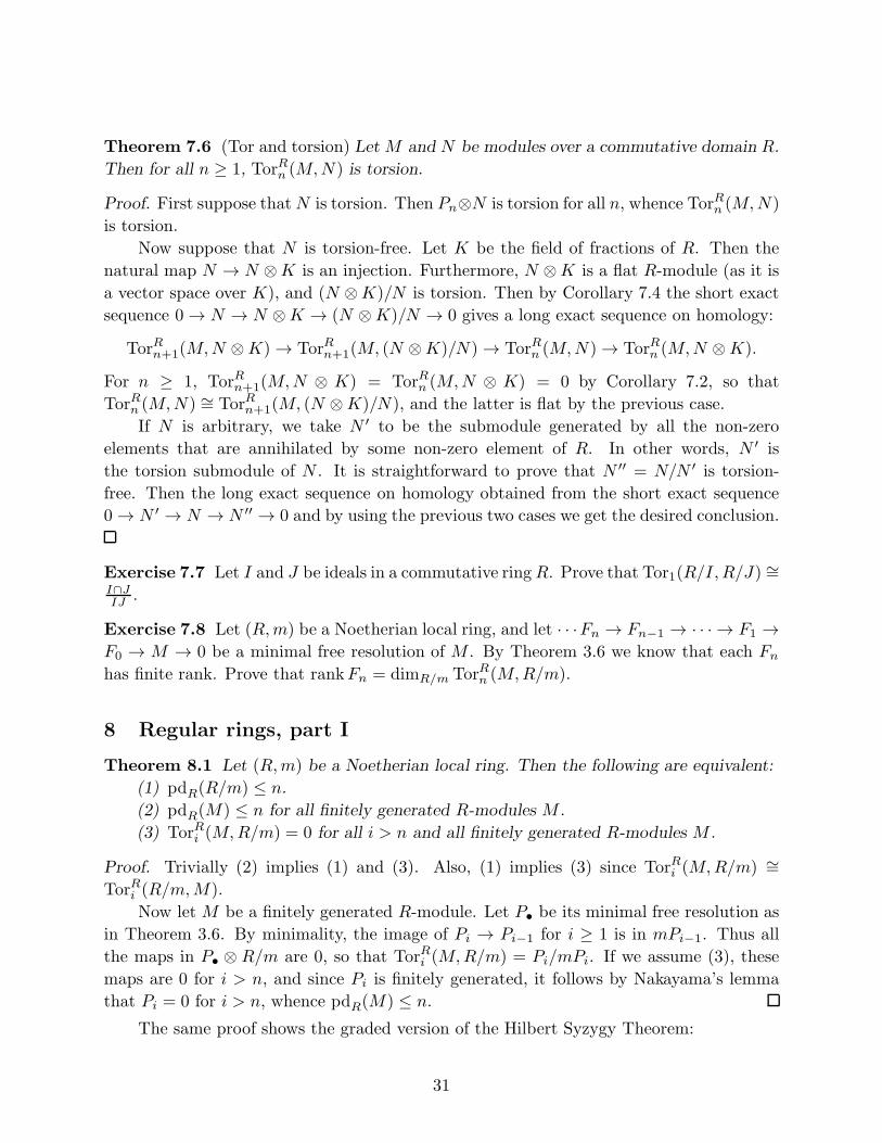
Theorem 7.6 (Tor and torsion) LetM and N be modules over a commutative domain R.
Then for all n ≥ 1, TorRn (M,N) is torsion.
Proof. First suppose thatN is torsion. Then Pn⊗N is torsion for all n, whence TorRn (M,N)
is torsion.
Now suppose that N is torsion-free. Let K be the field of fractions of R. Then the
natural map N → N ⊗K is an injection. Furthermore, N ⊗K is a flat R-module (as it is
a vector space over K), and (N ⊗K)/N is torsion. Then by Corollary 7.4 the short exact
sequence 0 → N → N ⊗K → (N ⊗K)/N → 0 gives a long exact sequence on homology:
TorRn+1(M,N ⊗K) → TorRn+1(M, (N ⊗K)/N) → TorRn (M,N) → TorRn (M,N ⊗K).
For n ≥ 1, TorRn+1(M,N ⊗ K) = TorRn (M,N ⊗ K) = 0 by Corollary 7.2, so that
TorRn (M,N) ∼= TorRn+1(M, (N ⊗K)/N), and the latter is flat by the previous case.
If N is arbitrary, we take N ′ to be the submodule generated by all the non-zero
elements that are annihilated by some non-zero element of R. In other words, N ′ isthe torsion submodule of N . It is straightforward to prove that N ′′ = N/N ′ is torsion-
free. Then the long exact sequence on homology obtained from the short exact sequence
0 → N ′ → N → N ′′ → 0 and by using the previous two cases we get the desired conclusion.
Exercise 7.7 Let I and J be ideals in a commutative ringR. Prove that Tor1(R/I, R/J) ∼=I∩JIJ .
Exercise 7.8 Let (R,m) be a Noetherian local ring, and let · · ·Fn → Fn−1 → · · · → F1 →F0 → M → 0 be a minimal free resolution of M . By Theorem 3.6 we know that each Fn
has finite rank. Prove that rankFn = dimR/m TorRn (M,R/m).
8 Regular rings, part I
Theorem 8.1 Let (R,m) be a Noetherian local ring. Then the following are equivalent:
(1) pdR(R/m) ≤ n.
(2) pdR(M) ≤ n for all finitely generated R-modules M .
(3) TorRi (M,R/m) = 0 for all i > n and all finitely generated R-modules M .
Proof. Trivially (2) implies (1) and (3). Also, (1) implies (3) since TorRi (M,R/m) ∼=TorRi (R/m,M).
Now let M be a finitely generated R-module. Let P• be its minimal free resolution as
in Theorem 3.6. By minimality, the image of Pi → Pi−1 for i ≥ 1 is in mPi−1. Thus all
the maps in P• ⊗ R/m are 0, so that TorRi (M,R/m) = Pi/mPi. If we assume (3), these
maps are 0 for i > n, and since Pi is finitely generated, it follows by Nakayama’s lemma
that Pi = 0 for i > n, whence pdR(M) ≤ n.
The same proof shows the graded version of the Hilbert Syzygy Theorem:
31
Theorem 8.2 Let R be a polynomial ring in n variables over a field. Then every graded
finitely generated R-module has finite projective dimension at most n.
Definition 8.3 A Noetherian local ring (R,m) is regular if pdR(R/m) <∞.
Definition 8.4 A Noetherian local ring (R,m) is regular if the minimal number of gen-
erators of m is the same as the Krull dimension of R.
It turns out that the two definitions of regularity coincide. We will prove this later
in Section 13. Naturally, the homological definition came on the scene much later. It is
difficult (or even impossible) to prove that a localization of a regular local ring at a prime
ideal is regular if we do not use the homological definition. But here is an easy proof of
this fact using the homological definition:
Theorem 8.5 Let (R,m) be a regular local ring, using Definition 8.3. Then for any prime
ideal P in R, RP is regular (under the same definition).
Proof. By Theorem 8.1, R/P has a finite projective resolution. Since a localization of a
projective module is projective and localization is flat, we get a finite projective resolution
of (R/P )P = RP /PRP . Hence by Theorem 8.1, since PRP is the unique maximal ideal of
RP , RP is regular.
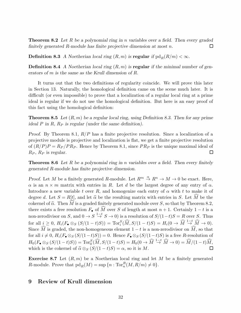
Theorem 8.6 Let R be a polynomial ring in n variables over a field. Then every finitely
generated R-module has finite projective dimension.
Proof. Let M be a finitely generated R-module. Let Rm α→ Rn →M → 0 be exact. Here,
α is an n × m matrix with entries in R. Let d be the largest degree of any entry of α.
Introduce a new variable t over R, and homogenize each entry of α with t to make it of
degree d. Let S = R[t], and let α be the resulting matrix with entries in S. Let M be the
cokernel of α. Then M is a graded finitely generated module over S, so that by Theorem 8.2,
there exists a free resolution F• of M over S of length at most n+ 1. Certainly 1 − t is a
non-zerodivisor on S, and 0 → S1−t→ S → 0) is a resolution of S/(1−t)S = R over S. Thus
for all i ≥ 0, Hi(F• ⊗S (S/(1 − t)S)) = TorSi (M, S/(1 − t)S) = Hi(0 → M1−t→ M → 0).
Since M is graded, the non-homogeneous element 1− t is a non-zerodivisor on M , so that
for all i 6= 0, Hi(F•⊗S (S/(1− t)S)) = 0. Hence F•⊗S (S/(1− t)S) is a free R-resolution of
H0(F• ⊗S (S/(1− t)S)) = TorS0 (M, S/(1− t)S) = H0(0 → M1−t→ M → 0) = M/(1− t)M ,
which is the cokernel of α⊗S (S/(1− t)S) = α, so it is M .
Exercise 8.7 Let (R,m) be a Noetherian local ring and let M be a finitely generated
R-module. Prove that pdR(M) = sup {n : TorRn (M,R/m) 6= 0}.
9 Review of Krull dimension
32
Definition 9.1 We say that P0 ( P1 ( · · ·( Pn is a chain of prime ideals if P0, . . . , Pn
are prime ideals. We also say that this chain has length n, and that the chain starts with
P0 and ends with Pn. This chain is saturated if for all i = 1, . . . , n there is no prime
ideal strictly between Pi−1 and Pi.
An example of a saturated chain of prime ideals is (0) ( (X1) ( (X1, X2) ( · · · ((X1, . . . , Xn) in k[X1, . . . , Xn], where k is a field and X1, . . . , Xn are variables. It is clear
that this is a chain of prime ideals, and to see that it is saturated between (X1, . . . , Xi−1)and (X1, . . . , Xi), we may pass to the quotient ring modulo (X1, . . . , Xi−1) and localize at
(X1, . . . , Xi), so that we are verifying whether a localization of k(Xi+1, . . . , Xn)[Xi] has
any prime ideals between (0) and (Xi). But since this ring is a principal ideal domain, we
know that there is no intermediate prime ideal.
In rings arising in algebraic geometry and number theory, namely in commutative
rings that are finitely generated as algebras over fields or over the ring of integers, whenever
P ⊆ Q are prime ideals, the length of any two saturated chains of prime ideals that start
with P and end with Q are the same. Rings with this property are called catenary. It
takes some work to prove that indeed these rings are catenary, and typically it is proved
via a strengthened form of the Noether normalization lemma in the case of fields or via
formal equidimensionality. We will not present a proof in class, but a reader may consult
Appendix B in [3].
Definition 9.2 The height (or codimension) of a prime ideal P is the supremum of all
the lengths of chains of prime ideals that end with P . The height (or codimension) of
an arbitrary ideal I is the infimum of all the heights of prime ideals that contain I . The
height of an ideal I is denoted as ht(I), and is either a nonnegative integer or ∞. The
(Krull) dimension of a ring R, denoted dimR, is the supremum of all the heights of
prime ideals in R.
The Krull dimension of a field is 0, the Krull dimension of a principal ideal domain
is 1. It is proved in Atiyah-MacDonald [1] that if R is commutative Noetherian, then for
any variable X over R, dimR[X] = dimR + 1. In particular, dim k[X1, . . . , Xn] = n, if k
is a field and X1, . . . , Xn are variables over k. Note that the Krull dimension of k[X]/(X2)
is 0, but that the k-vector space dimension is 2.
Theorem 9.3 (Krull Principal Ideal Theorem, or Krull’s Height Theorem) Let R be
a Noetherian ring, let x1, . . . , xn ∈ R, and let P be a prime ideal in R minimal over
(x1, . . . , xn). Then htP ≤ n.
Proof. Height of a prime ideal does not change after localization at it, so we may assume
without loss of generality that P is the unique maximal ideal in R.
The case n = 0 is trivial, then P is minimal over the ideal generated by the empty
set, i.e., P is minimal over (0), so P is a minimal prime ideal, no prime ideal is strictly
contained in it, so that htP = 0.
33
Next we prove the case n = 1. Suppose that there exist prime ideals P0(Q(P . Since
P is minimal over (x1), It follows that R/(x1) has only one prime ideal, so that R/(x1) is
Artinian. It follows that the descending sequence
Q+ (x1) ⊇ Q2RQ ∩R+ (x1) ⊇ Q3RQ ∩R+ (x1) ⊇ · · ·
stabilizes somewhere, so there exists n such that Qn+1RQ ∩R+ (x1) = QnRQ ∩R+ (x1).
Thus QnRQ∩R ⊆ (Qn+1RQ∩R+(x1))∩QnRQ∩R = Qn+1RQ∩R+(x1)∩QnRQ∩R. SinceQnRQ is primary in RQ,* it follows that QnRQ ∩R is primary in R. Since x1 is not in Q,
x1 is a non-zerodivisor modulo the Q-primary ideal QnRQ ∩R, so that (x1)∩QnRQ ∩R =
x1(QnRQ∩R). Hence QnRQ∩R ⊆ Qn+1RQ∩R+x1(Q
nRQ∩R), and even equality holds.
Thus by Nakayama’s lemma, QnRQ ∩ R = Qn+1RQ ∩ R, so that QnRQ = Qn+1RQ, and
so by Nakayama’s lemma again, QnRQ = 0. This says that in the Noetherian local ring
RQ the maximal ideal is nilpotent, so that RQ is Artinian and QRQ has height 0, which
contradicts the existence of P0.
Now let n ≥ 2. Let P0 ( P1 ( P2 ( · · · ( Pn ( P be a chain of prime ideals. If
x1 ∈ P0, then P/P0 is minimal over the ideal (x2, . . . , xn)(R/P0), so that by induction on n,
ht(P/P0) ≤ n−1, which contradicts the existence of the chain above. So x1 6∈ P0. Let i be
the smallest integer such that x1 ∈ Pi+1 \ Pi. We just proved that i ∈ {0, . . . , n}. Supposethat i > 1. Then by denoting P as Pn+1, in the Noetherian local domain RPi+1
/Pi−1RPi+1,
the maximal ideal has height at least 2 and it contains the non-zero image of x1. By primary
decomposition there exists a prime ideal Q in this domain that is minimal over the image
of (x1), and by the case n = 1, the height of that prime ideal is at most 1, and since Q
cannot be the minimal prime ideal as it contains a non-zero element, it follows that the
height of Q is 1. Note that Q lifts to R to a prime ideal strictly between Pi−1 and Pi+1
that contains x1. So by possibly replacing Pi with Q, we may assume that x1 ∈ Pi, and
by repetition of this argument, we may assume that x1 ∈ P1. The prime ideal P/P1 is
minimal over (x2, . . . , xn)(R/P1), so that by induction on n, ht(P/P1) ≤ n−1, which gives
a contradiction to the existence of the long chain of prime ideals.
Corollary 9.4 Every prime ideal in a Noetherian ring has finite height.
Proof. Since every ideal is finitely generated, by Theorem 9.3 its height is at most the
(finite) number of generators.
Thus every Noetherian local ring is finite-dimensional, but there exist Noetherian rings
that are not finite-dimensional.
For a converse of the Krull Principal Ideal Theorem we will need a form of the Prime
Avoidance Theorem, see Exercise 9.12.
* A review of primary modules is in Section 10.
34
Theorem 9.5 (A converse of the Krull Principal Ideal Theorem) Let R be a Noetherian
ring, and let P be a prime ideal in R of height n. Then there exist x1, . . . , xn ∈ P such
that P is minimal over (x1, . . . , xn).
Proof. By localizing without loss of generality we may assume that R is a Noetherian local
ring in which P is the only maximal ideal.
If the height of P is 0, there is nothing to do, as P is minimal over the ideal generated
by the empty set.
Now suppose that n > 0. By primary decomposition results we know that R has only
finitely many minimal primes. By Prime Avoidance there exists x1 ∈ P that avoids all
these finitely many minimal primes. If P has height 1, it is the only prime ideal in addition
to the minimal prime ideals, so that P is minimal over (x1), as desired. So suppose that
P has height n > 1. By primary decomposition there exist finitely many prime ideals
in R that are minimal over (x1). Let x2 ∈ P avoid all these finitely many primes. If
n = 2, P is the only prime ideal in R that contains (x1, x2), so that P is minimal over the
two-generated ideal (x1, x2), as desired. If n > 2, continue by finding x3 ∈ P that avoids
all the prime ideals in R that are minimal over (x1, x2), etc. We stop after we construct
x1, . . . , xn ∈ P such that P is minimal over (x1, . . . , xn).
Note that a modified form of the Krull Principal Ideal Theorem says that if a prime
ideal in a Noetherian ring is minimal over an ideal generated by a regular sequence of
length n, then the height of that prime ideal is exactly n.
Definition 9.6 Let R be a commutative ring and let M be an R-module. The Krull
dimension of M is dim(R/ann(M)).
Proposition 9.7 Let (R,m) be a Noetherian local ring and let M be a finitely generated
R-module. Then M has finite Krull dimension, and dimM is the smallest number n of
elements x1, . . . , xn inm such that (x1, . . . , xn)+annM ism-primary. Or equivalently, htm
is the smallest number n of elements x1, . . . , xn ∈ m such that (x1, . . . , xn) is m-primary.
Proof. We only prove the second part, but that follows from the Krull Principal Ideal
Theorem and its converse.
Proposition 9.8 Let (R,m) be a Noetherian local ring and let M be a finitely generated
R-module of positive dimension. Let x ∈ m not be in any prime ideal minimal over ann(M).
Then dim(M/xM) = dimM − 1.
Proof. Left to the reader.
35
Proposition 9.9 Let (R,m) be a Noetherian local ring and let 0 →M ′ →M →M ′′ → 0
be a short exact sequence of finitely generated R-modules. Then
(1) dimM ≤ max {dimM ′, dimM ′′},(2) dimM ′, dimM ′′ ≤ dimM .
Proof. Let x1, . . . , xn ∈ m. By the right-exactness of the tensor product, tensoring with
R/(x1, . . . , xn) yields the following exact complex:
M ′/(x1, . . . , xn)M′ →M/(x1, . . . , xn)M →M ′′/(x1, . . . , xn)M
′′ → 0.
By the proof (!) of the converse of the Krull Principal Ideal Theorem, we may choose
x1, . . . , xn such that n = max {dimM ′, dimM ′′} so that (x1, . . . , xn) + annM ′ and
(x1, . . . , xn) + annM are m-primary. This means that the modules M ′/(x1, . . . , xn)M ′
and M ′′/(x1, . . . , xn)M ′′ have dimension 0, i.e., that they have finite length. But then the
middle module M/(x1, . . . , xn)M also has finite length, so that (x1, . . . , xn) + annM is
m-primary, whence dimM ≤ n. This proves (1).
Now suppose that x1, . . . , xn are chosen so that n = dimM and (x1, . . . , xn) +
annM is m-primary. Then M/(x1, . . . , xn)M has finite length, and so necessarily
M ′′/(x1, . . . , xn)M ′′ has finite length, which proves that dimM ′′ ≤ dimM . But with our
homological algebra, we can extend the displayed exact complex above further:
TorR1 (M′′, R/(x)) →M ′/(x)M ′ →M/(x)M →M ′′/(x)M ′′ → 0.
Since (x) + annM ′′ ⊆ ann TorR1 (M′′, R/(x)) by Property 7. of Tor, we have that
TorR1 (M′′, R/(x)) has finite length, so that M ′/(x)M ′ has finite length, whence
dimM ′ ≤ n. This finishes the proof of (2).
Definition 9.10 We have seen that in a Noetherian local ring (R,m), m is minimal over
an ideal generated by dimR elements. Note that such an ideal is m-primary. Any sequence
of dimR elements that generate an m-primary ideal is called a system of parameters.
Obviously, every system of parameters in a Noetherian local ring has the same length.
Exercise 9.11 Let P ′′ ⊆ P ′ be prime ideals in a Noetherian ring with at least one in-
termediate prime ideal. Prove that there exist infinitely many prime ideals between P ′′
and P ′. (Hint: adapt the proof of Theorem 9.3.)
Exercise 9.12 (Prime Avoidance) Let I be an ideal contained in the union ∪ni=1Pn, where
P1, . . . , Pn are ideals, at most two of which are not prime. Prove that I is contained in one
of the Pi. Strengthened form: if I is contained in the Jacobson radical of I and all the Pi
except possibly one are prime ideals, then there exists a minimal generator y of I that is
not contained in any Pi.
36
Exercise 9.13 Find an example of a Noetherian ring of infinite Krull dimension.
Exercise 9.14 Let (R,m) be a Noetherian local ring, and let M be a finitely generated
R-module of dimension d. Let x1, . . . , xn ∈ m. Then M/(x1, . . . , xn)M has dimension at
least n− k.
Exercise 9.15 Let (R,m) be a Noetherian local ring, of dimension d. Suppose that
m = (x1, . . . , xd).
(1) Prove that R is a field if d = 0.
(2) Prove that R is a principal ideal domain if d = 1.
10 Regular sequences
Recall Definition 5.4: x1, . . . , xn ∈ R is a regular sequence on a module M if
(x1, . . . , xn)M 6=M and if for all i = 1, . . . , n, xi is a non-zerodivisor onM/(x1, . . . , xi−1)M .
We say that this regular sequence has length n.
It is not clear that x1, . . . , xn being a regular sequence forces these elements to form
a regular sequence in any order. In fact, it is not true in general. The standard example
is the regular sequence x, (x− 1)y, (x− 1)z in the polynomial ring k[x, y, z] over a field k;
the permutation (x− 1)y, (x− 1)z, x is not a regular sequence.
Definition 10.1 Let R be a commutative ring, M an R-module and I an ideal in R. The
I-depth of M or the grade of M with respect to I , is the supremum of the lengths of
sequences of elements in I that form regular sequences on M . We denote it by depthI(M).
If (R,m) is local, the depth of M is the m-depth of M .
The following are some straightforward facts:
(1) If x1, x2, . . . ∈ I is a regular sequence on M , then for all n, (x1, . . . , xn)M (
(x1, . . . , xn+1)M .
(2) If M is Noetherian, then depthI(M) <∞.
(3) For any Noetherian ring R, for any proper ideal I , and any finitely generated
R-module M , depthI M ≤ dimM, ht I .
We would like a parallel to Theorem 9.5 for sequences giving correct height. It is
not enough to simply avoid all the minimal primes, we need to avoid zerodivisors. To
understand the structure of zerodivisors, we first need a quick detour into primary decom-
positions.
Here is a quick review of the theory in case R is Noetherian and M is a finitely
generated module over R.
(4) A submodule N of M is said to be primary if N 6= M and whenever r ∈ R,
m ∈M \N , and rm ∈ N , then there exists a positive integer n such that rnM ⊆
37
N . In other words, N is primary in M if and only if for any r ∈ R, whenever
multiplication by r on M/N is not injective, then it is nilpotent as a function.
(5) If N ⊆ M is a primary submodule, then√N :R M is a prime ideal. In this case
we call N is also called P -primary, where P =√N :R M . Then also N :R M is
a P -primary ideal.
(6) The intersection of any finite set of P -primary submodules of M is P -primary.
(7) If N ⊆M is a P -primary submodule, then for any r ∈ R,
N :M r =
N, if r 6∈ P ;M, if r ∈ N :R M ;a P -primary submodule of M strictly containing N, if r ∈ P \ (N :R M),
and for any m ∈M ,
N :R m =
{R, if m ∈ N ;a P -primary ideal containing N :R M, if m 6∈ N.
Moreover, there exists m ∈M such that N : m = P .
(8) If is U a multiplicatively closed subset of R, and N ⊆ M is P -primary, such that
U ∩ P = ∅, then U−1N is U−1P -primary in U−1M .
(9) Every submodule N of M can be written as a finite intersection of primary sub-
modules. If we remove redundancies, the set of prime ideals P such that a P -
primary submodule appears in the decomposition is uniquely determined. Such
prime ideals are called associated primes of N , and their set is usually denoted
Ass(M/N).
(10) If N = ∩iNi is a (minimal) primary decomposition of N inM , then 0 = ∩i(Ni/N)
is a (minimal) primary decomposition of 0 in M/N , and of course the set of
associated primes of N in M is the set of associated primes of 0 in M/N .
(11) The prime ideals that are minimal over ann(M) are called minimal prime ideals
of M , and the set of all such is denoted Min(M). This set is always contained in
Ass(M).
(12) For any P ∈ MinM , the P -primary component of 0 in M is ker(M →MP ). This
is uniquely determined. The embedded components are not uniquely determined.
(13) The set of zero divisors on M/N equals⋃
P∈Ass(M/N)
P .
38
Proposition 10.2 (How to construct a regular sequence) Let R be a Noetherian ring, let
I be an ideal in R, and let M be a finitely generated R-module. Then a regular sequence
x1, . . . , xn ∈ I on M can be constructed as follows: If I is contained in some prime ideal
associated to annM (i.e., to M), then all regular sequences in I on M have length 0, and
we are done. Othewise, we first choose x1 ∈ I that is not in any prime ideal associated to
annM (i.e., to M). We can do this by Prime Avoidance. If I is contained in some prime
ideal associated toM/(x1)M , i.e., to (x1)+annM , then we stop at x1, otherwise we may by
Prime Avoidance choose x2 ∈ I that is not contained in any prime ideal associated to (x1).
If I is contained in some prime ideal associated to M/(x1, x2)M , i.e., to (x1, x2) + annM ,
then we stop at x1, x2, otherwise we may by Prime Avoidance choose x3 ∈ I that is not
contained in any prime ideal associated to (x1, x2). And we continue in this way.
Clearly this procedure constructs some regular sequence, and it must terminate. What
is not clear that all choices of x1, . . . , xn of maximal length have the same length. We give
an elementary proof of this fact in Proposition 10.7.
We can detect the existence of some regular sequences via Koszul complexes:
Proposition 10.3 Let R be a Noetherian ring, let M be a finitely generated R-module,
and let x1, . . . , xn be contained in the Jacobson radical of R. If Hi(K•(x1, . . . , xn;M) = 0
for i = n, n − 1, . . . , n − l + 1, then there exists y1, . . . , yn ∈ R such that (x1, . . . , xn) =
(y1, . . . , yn) and y1, . . . , yl is a regular sequence on M .
Proof. If l = 0, there is nothing to prove. So we may assume that l > 0. We will use
Exercise 1.3 that says that Hn(K•(x1, . . . , xn;M)) = annM (x1, . . . , xn) for all x1, . . . , xnand M . By assumption, annM (x1, . . . , xn) = 0, so that (x1, . . . , xn) is not contained
in any prime ideal that is associated to M . Thus by the strengthened form of Prime
Avoidance, there exists y1 ∈ (x1, . . . , xn) that is a minimal generator of the ideal such that
annM (y1) = 0. In other words, y1 is a non-zerodivisor on M . By Exercise 5.7 we may
assume that y1 = x1: all the hypotheses are still satisfied. If l = 1, we are done. Otherwise,
Equation (5.3) implies that for all Hi(K•(x2, . . . , xn;M))/x1Hi(K•(x2, . . . , xn;M)) = 0.
Thus by Nakayama’s lemma, Hi(K•(x2, . . . , xn;M)) = 0 for i = n, n−1, . . . , n−l+1. Since
Hn(K•(x2, . . . , xn;M)) = 0 trivially as n is strictly larger than the number of elements in
{x2, . . . , xn}, this really simply says that Hi(K•(x2, . . . , xn;M)) = 0 for i = n− 1, . . . , n−l + 1. Then by induction on n the conclusion follows.
Proposition 10.4 Let x1, . . . , xn be in the Jacobson radical of a Noetherian ring. Suppose
that x1, . . . , xn is a regular sequence on a finitely generated R-module M . Then for any
permutation π ∈ Sn and for any positive integers m1, . . . , mn, xm1
π(1), . . . , xmn
π(n) is a regular
sequence on M .
Proof. There are two issues here: we may permute the elements x1, . . . , xn, and we may
take them to different powers. To prove that the permutation works, it suffices to prove
the case when we permute two consecutive elements, i.e., it suffices to prove that if a, b is a
39
regular sequence onM , so is b, a. If ax = by for some x, y ∈M , then by assumption y = az
for some z ∈ M , so that a(x − bz) = 0, and since a is a non-zerodivisor on M , x = bz.
Thus a is a non-zerodivisor on M/bM . If bx = 0 for some x ∈ M , then bx ∈ aM , so by
assumption x ∈ aM . Write x = ax1 for some x1 ∈M . Then 0 = bx = bax1, and since a is
a non-zerodivisor on M , bx1 = 0. By repeating this process, we get that x1 ∈ aM , whence
x ∈ a2M , so that x ∈ ∩akM = 0. This proves that b, a is a regular sequence on M , and so
more generally, that xπ(1), . . . , xπ(n) is a regular sequence on M .
It remains to prove that xm1
1 , . . . , xmnn is a regular sequence on M . If xn is a non-
zerodivisor on M/(x1, . . . , xn−1)M , so is xmnn , so that x1, . . . , xn−1, xmn
n is a regular se-
quence on M . Hence by the previous paragraph, xmnn , x1, . . . , xn−1 is a regular sequence,
and by induction we may raise x1, . . . , xn−1 to various powers and still preserve the regular
sequence property, whence by the previous paragraph x1, . . . , xn with imposed arbitrary
powers form a regular sequence on M .
Note that the proof above shows more:
Corollary 10.5 Whenever a, b is a regular sequence onM and b is a non-zerodivisor onM ,
then b, a is a regular sequence on M .
Proposition 10.6 Let R be a Noetherian ring, let I be an ideal in R, and let M be a
finitely generated R-module of depth k. If x1, . . . , xk ∈ I is a maximal regular sequence,
there exists w ∈M \ (x1, . . . , xk)M such that wI ⊆ (x1, . . . , xk)M .
Proof. It suffices to prove that if M has I-depth zero, then there exists a non-zero element
w ∈ M such that Iw = 0. The assumption on I-depth zero implies that I is contained in
an associated prime ideal P of M , so that there exists w ∈ M such that P = (0M) : w.
Hence Iw ⊆ Pw = 0.
Proposition 10.7 Let I be an ideal in a Noetherian ring R. LetM be a finitely generated
R-module. Let x1, . . . , xn ∈ I be a maximal regular sequence on M . Then every maximal
regular sequence on M of elements in I has length n.
Proof. Let y1, . . . , ym ∈ I be another regular sequence on M . Without loss of generality
n ≤ m. If n = 0, this says that I consists of zerodivisors on M , so that m = 0 as well.
Suppose that n = 1. Then I consists of zerodivisors on M/x1M . By Proposition 10.6
there exists w ∈ M \ x1M such that Iw ⊆ x1M . Thus y1w = x1w′ for some w′ ∈ M .
If w′ ∈ y1M , then w ∈ x1M , which is not the case, so necessarily w′ 6∈ y1M . Also,
Ix1w′ = y1Iw ⊆ y1x1M , so that Iw′ ⊆ y1M , so that I consists of zerodivisors on M/y1M .
Thus m = 1 as well.
Now suppose that n > 0 and that m > n. Then there exists c ∈ I that is not con-
tained in any associated primes of M , M/(x1)M , M/(x1, x2)M , . . ., M/(x1, . . . , xn−1)M ,
M/(y1)M , M/(y1, y2)M , . . ., M/(y1, . . . , yn)M . Then x1, . . . , xn−1, c and y1, . . . , yn, c areregular sequences on M . Since x1, . . . , xn is a maximal M -regular sequence in I , by pos-
sibly first passing to M/(x1, . . . , xn−1)M , the case n = 1 says that that x1, . . . , xn−1, c
40
is also a maximal M -regular sequence in I . Thus by Corollary 10.5, c, x1, . . . , xn−1 and
c, y1, . . . , yn are regular sequences on M , and necessarily c, x1, . . . , xn−1 is a maximal M -
regular sequence in I . It follows that x1, . . . , xn−1 and y1, . . . , yn are regular sequences on
M/cM , with the first sequence maximal, and so by induction on n, n ≤ n− 1, which gives
a contradiction. Thus m ≤ n, and by the minimality of n, m = n.
We can make Proposition 10.6 more precise:
Proposition 10.8 Let (R,m) be a Noetherian local ring and letM be a finitely generated
R-module of depth k. Let x1, . . . , xk ∈ m form a regular sequence on M . Then
(1) m is associated to M/(x1, . . . , xk)M ,
(2) there exists w ∈M/(x1, . . . , xk)M such that m = ann(w),
(3) and there exists an injection R/m→M/(x1, . . . , xk)M (taking 1 to w).
Proof. If the (finite) set of associated primes ofM/(x1, . . . , xk)M does not include m, then
by Prime Avoidance we can find xk+1 ∈ m which is a non-zerodivisor onM/(x1, . . . , xk)M ,
which contradicts the definition of depth of M being k. Thus m is associated to M/(x)M ,
i.e., to (x) + annM . This means that m = ((x) + annM) : y. Then ymM ⊆ ((x) +
annM)M = (x)M . If yM ⊆ (x)M , then y ∈ (x) + annM , which contradicts that m =
((x) + annM) : y.
Then zm ∈ (x)M , so that m ⊆ ((x)M : z) ( R, so that m = ((x)M : z). Now set w
to be the image of z in M/(x)M . The rest is easy.
Exercise 10.9 Prove that if x ∈ I is a non-zerodivisor on M , then depthI(M/xM) =
depthI(M)− 1.
Exercise 10.10 Prove that depthI(M ⊕N) = min {depthI(M), depthI(N)}.
Exercise 10.11 Prove that depthI(M) = depth√I(M).
Exercise 10.12 Let R be a Noetherian commutative ring and let I be a proper ideal in R.
Suppose that I is generated by a regular sequence. Prove that I/I2 is a free (R/I)-module
and that R/I has finite projective dimension over R. (See also Exercise 13.13.) (Hint:
Koszul complex for the last part.)
11 Regular sequences and Tor
41
Proposition 11.1 Let M and N be finitely generated modules over a Noetherian local
ring (R,m), and suppose that M has finite projective dimension n and that m ∈ AssN .
Then TorRn (M,N) 6= 0.
Proof. Since m ∈ AssN , there exists a short exact sequence 0 → R/m → N → L → 0.
Then we get the induced long exact sequence on Tor, with the relevant part being
TorRn+1(M,L) → TorRn (M,R/m) → TorRn (M,N).
SinceM has projective dimension n, TorRn+1(M,L) = 0, and by Exercise 8.7, TorRn (M,R/m) 6=0. Hence by the exactness of the complex above, TorRn (M,N) 6= 0.
Corollary 11.2 Let (R,m) be a Noetherian local ring, let M and N be finitely gener-
ated R-modules of finite projective dimension such that m is associated to both. Then
pdR(M) = pdR(N).
Proof. Let n = pdM and let n′ = pdN . By Proposition 11.1, TorRn (M,N) 6= 0, so that
n′ ≥ n. By symmetry, n ≥ n′.
In general the depth of a Noetherian local ring can be strictly smaller than the depth
of some finitely generated module. For example, Let R = k[[x, y]]/(x2, xy) andM = R/(x).
Then R is a Noetherian local ring of depth 0, but y ∈ R is a non-zerodivisor on M , so that
depthM ≥ 1. See the contrast with the proposition below:
Proposition 11.3 Let (R,m) be a Noetherian local ring and letM be a finitely generated
R-module of finite projective dimension. Then depthM ≤ depthR.
Proof. Suppose that d = min {depthR, depthM} = depthR. By Proposition 10.2, there
exists a sequence x1, . . . , xd ∈ m that is regular on R and on M . By Exercise 5.6,
K•(x1, . . . , xd;R) is a free resolution of R/(x1, . . . , xd), and K•(x1, . . . , xd;M) is a free
resolution of M/(x1, . . . , xd)M .
Let n = pdR(M). By Proposition 10.8, m is associated to R/(x1, . . . , xd), and so by
Proposition 11.1,
Hn(K•(x1, . . . , xd;M)) = Hn(M ⊗K•(x1, . . . , xd;R)) = TorRn (M,R/(x1, . . . , xd))
is non-zero. Thus n = 0. But then M is a projective R-module, and hence free, whence
depthM = depthR.
42
Proposition 11.4 Let (R,m) be a Noetherian local ring, let M be a finitely generated
R-module of projective dimension n, and let x ∈ R be a non-zerodivisor on R.
(1) If x is a non-zerodivisor onM , thenM/xM has projective dimension n over R/xR.
(2) In general, if K = ker(Rµ(M) → M) then K/xK has projective dimension n − 1
over R/xR.
Proof. Let 0 → Fn → Fn−1 → · · · α→ F1 → F0 →M → 0 be exact, where all Fi are finitely
generated projective and hence free over R, and where for all i ≥ 0, the map Fi+1 → Fi
has image in mFi. If we tensor this with R/(x), we get the complex
0 → Fn
xFn→ Fn−1
xFn−1→ · · · α→ F1
xF1→ F0
xF0→ 0.
Its homology at the ith place for i > 0 is TorRi (M,R/(x)). Since R/(x) has projective
dimension 1, the displayed complex has zero homology at places i ≥ 2. Also,
TorR0 (M,R/(x)) = H0(M ⊗ (0 → Rx→ R → 0)) = H0(0 →M
x→ M → 0) =M/xM,
and
TorR1 (M,R/(x)) = H1(M ⊗ (0 → Rx→ R → 0)) = H1(0 →M
x→ M → 0) = (0 :M x).
If x is a non-zerodivisor on M , then TorR1 (M,R/(x)) = 0, so that
0 → Fn
xFn→ Fn−1
xFn−1→ · · · α→ F1
xF1→ F0
xF0→ M
xM→ 0,
is exact (the last part by right exactness by tensoring with R/(x)). So we got a finite free
resolution of M/xM over R/(x) and since the original resolution of M was minimal, so is
this one, which means that the projective dimension of M/xM over R/xR is n.
In general,
0 → Fn
xFn→ Fn−1
xFn−1→ · · · α→ F1
xF1→ F1
xF1 + imα→ 0
is exact, giving a minimal finite free resolution of F1
xF1+imα over R/(x). However, by
construction of resolutions, F1
imα∼= K, so that F1
xF1+imα∼= K
xK. This proves that the
projective dimension of K/xK over R/xR is n− 1.
43
Theorem 11.5 (Auslander-Buchsbaum formula) Let (R,m) be a Noetherian local ring,
and letM be a finitely generated R-module of finite projective dimension. Then pdR(M)+
depthM = depthR.
Proof. First suppose that depthM = 0. Then by Proposition 10.8, m is associated to M .
Let d = depthR. There exists x1, . . . , xd ∈ m that form a regular sequence on R. Then
again by Proposition 10.8, m is associated to R/(x1, . . . , xd). Since R/(x1, . . . , xd) also
has a minimal finite free resolution via the Koszul complex of length d, so its projective
dimension is d. By Corollary 11.2, depthR = d = pdM = pdM + depthM .
Now suppose that depthM > 0. By Proposition 11.3 depthR > 0. Thus by Propo-
sition 10.2 there exists x ∈ m that is a non-zerodivisor on M and on R. By Proposi-
tion 11.4,M/xM has finite projective dimension over R/xR, and this projective dimension
equals pdM . Also, M/xM has depth exactly one less than depthM , and depthR/(x) =
depthR− 1, whence by induction on depthR we get the desired equality.
Exercise 11.6 Go through this section and remove the finitely generated assumption
wherever possible.
12 Cohen–Macaulay rings and modules
Definition 12.1 A Noetherian local ring (R,m) is Cohen–Macaulay if m contains a
regular sequence of length equal to the dimension of R. More generally, a finitely generated
R-module M is Cohen–Macaulay if depthM = dimM .
A Noetherian ring R is Cohen–Macaulay if all of its localizations at maximal ideals
are Cohen–Macaulay. A finitely generated R-moduleM over a Noetherian ring is Cohen–
Macaulay if for all maximal ideals m in R, Mm is a Cohen–Macaulay Rm-module.
The following are again easy facts:
(1) Z, principal ideal domains, and fields are Cohen–Macaulay.
(2) Every 0-dimensional Noetherian ring is Cohen–Macaulay.
(3) Every 1-dimensional Noetherian domain is Cohen–Macaulay.
(4) Let (R,m) be a Noetherian local ring, let M be a Cohen–Macaulay R-module,
and let x1, . . . , xn ∈ m form a regular sequence on M . Then M/(x1, . . . , xn)M is
Cohen–Macaulay.
(5) In a Cohen–Macaulay local ring, some system of parameters forms a regular se-
quence. Also, every maximal regular sequence in m is a system of parameters.
44
Theorem 12.2 The following are equivalent for a Noetherian local ring (R,m):
(1) R is Cohen–Macaulay.
(2) Some system of parameters in R forms a regular sequence.
(3) Every system of parameters in R forms a regular sequence.
Proof. Clearly (1) is equivalent to (2), and (3) implies both (1) and (2). Now suppose
that (1) and (2) hold. Let d = dimR and let y1, . . . , yd be a system of parameters. We
need to prove that y1, . . . , yd is a regular sequence. If d = 0, there is nothing to prove.
If d = 1, then R has only finitely many primes: all the minimal primes and m. Since
by (2) m contains a non-zerodivisor, all zerodivisors live in the union of the set of all
minimal primes. Since y1 is a parameter in a one-dimensional ring, it is not in any minimal
prime, but then it is not a zerodivisor. This proves the case d = 1. Now let d > 1.
Let x1, . . . , xd be a system of parameters that is a regular sequence. By construction of
non-zerodivisors and parameters, since it is a matter of avoiding finitely many primes that
do not contain m, there exists c ∈ m such that x1, . . . , xd−1, c is a regular sequence and
such that y1, . . . , yd−1, c is a system of parameters. By Proposition 10.4, c, x1, . . . , xd−1is a regular sequence, and certainly c, y1, . . . , yd−1 is a system of parameters. Since c is a
non-zerodivisor, dim(R/(c)) = dimR−1 and depth(R/(c)) = depthR−1. Thus R/(c) is a
Cohen–Macaulay ring. By induction on d, then y1, . . . , yd1is a regular sequence on R/(c),
so that c, y1, . . . , yd−1 is a regular sequence in R. Again by Proposition 10.4, y1, . . . , yd−1, cis a regular sequence, and then by passing to R/(y1, . . . , yd−1) and the case d = 1, y1, . . . , ydis a regular sequence.
Corollary 12.3 Let (R,m) be a Cohen–Macaulay local ring and let P be a prime ideal
in R. Then RP is a Cohen–Macaulay local ring, and htP + dim(R/P ) = dimR.
Furthemore, if x1, . . . , xd is any regular sequence, than any prime ideal associated to
(x1, . . . , xd) is minimal over the ideal.
Proof. Certainly by the definition of dimension, we always have htP + dim(R/P ) ≤dimR = d.
By Theorem 9.5, actually by its proof, there exists a part of a system of parameters
x1, . . . , xn ∈ P such that P is minimal over (x1, . . . , xn) and n = htP . These can be
extended to a system of parameters x1, . . . , xd. By Theorem 12.2, x1, . . . , xd is a regular
sequence. Thus P is minimal over the ideal generated by a regular sequence x1, . . . , xn,
whence PRP is minimal over an ideal generated by a regular sequence, so that by the
theorem, RP is Cohen–Macaulay. It remains to prove the dimension/height equality.
We will prove more generally that if P ∈ Ass(R/(x1, . . . , xn)), where x1, . . . , xd is a
regular sequence, then dim(R/P ) = d − n. If we prove that, then since htP ≥ n, by the
inequality in the first part, htP = n.
If n = d, there is nothing to prove. So suppose that n < d. Let J = ((x1, . . . , xn) :
P ) ⊆ J ′ = ((x1, . . . , xn, xn+1) : P ). By Proposition 10.6 J is properly contains (x1, . . . , xn).
Suppose that J ′ = (x1, . . . , xn+1). Then for all w ∈ J(⊆ J ′), w =∑n−1
i=1 xizi for some
45
zi ∈ R, whence Pw ⊆ (x1, . . . , xn) means that Pzn+1 ⊆ (x1, . . . , xn), so that zn+1 ∈ J
and w ∈ (x1, . . . , xn) + xn+1J . Thus by Nakayama’s lemma, J = (x1, . . . , xn), which is a
contradiction. Thus J ′ properly contains (x1, . . . , xn+1). So P consists of zerodivisors on
R/(x1, . . . , xn+1). Let Q be a prime ideal associated to R/(x1, . . . , xn+1) that contains P .
But xn+1 is in Q and not in P , so that P 6= Q. Also, Q is associated to (x1, . . . , xn+1), so
that by induction on d − n, dim(R/Q) = d − n − 1. But then dim(R/P ) ≥ dim(R/Q) +
1 = d − n, but always dim(R/P ) + htP ≤ dimR = d, from which we conclude that
dim(R/P = d− n = dimR− htP .
Exercise 12.4 Prove that Q[[x2, x3]] is Cohen–Macaulay but is not regular either by
Definition 8.3 or by Definition 8.4.
Exercise 12.5 Prove that Q[x, y, u, v]/(x, y)(u, v) is not Cohen–Macaulay.
Exercise 12.6 Prove that a localization of a Cohen–Macaulay module is Cohen–Macaulay.
Exercise 12.7 Let R be a Cohen–Macaulay local ring. Prove that for any system of
parameters x1, . . . , xd, R/(x1, . . . , xd) has finite projective dimension.
Exercise 12.8 Let R be a Cohen–Macaulay ring. Prove that for any variables X1, . . . , Xn
over R, R[X1, . . . , Xn] is Cohen–Macaulay. (If you get stuck, look at Examples 13.4.)
13 Regular rings, part II
Here we tie some loose ends from Section 8.
Proposition 13.1 Let R be a Noetherian ring. Suppose that P = (x1, . . . , xd) is a prime
ideal of height d that lies in the Jacobson radical. Then (x1, . . . , xd−1) is a prime ideal.
Proof. Let q be a prime ideal minimal over J contained in P . By the generalized Krull
principal ideal theorem, q 6= P . Suppose that q 6= J . Let a ∈ q \ J . Since q ⊆ P , we can
write a = j1 + a1xd for some j1 ∈ J and some a1 in R. Then a1xd ∈ q, and since xd 6∈ q,
it follows that a1 ∈ q. Then we can write a1 in a similar way as a, and an iteration of this
gives that for all n ≥ 1, a = jn + anxnd for some jn ∈ J and some an in R. But then since
R is local, a ∈ J , which is a contradiction. This proves that J is a prime ideal, strictly
contained in P .
46
Theorem 13.2 Let (R,m) be a Noetherian local ring. Then the following are equivalent:
(1) pdR(R/m) = dimR.
(2) pdR(M) ≤ dimR for all finitely generated R-modules M .
(3) TorRi (M,R/m) = 0 for all i > dimR and all finitely generated R-modules M .
(4) pdR(R/m) ≤ n for some integer n.
(5) pdR(M) ≤ n for all finitely generated R-modules M for some integer n.
(6) There exists an integer n such that TorRi (M,R/m) = 0 for all i > n and all finitely
generated R-modules M .
(7) Every minimal generating set of m is a regular sequence.
(8) m is generated by a regular sequence.
(9) The minimal number of generators of m equals the dimension of R.
Proof. We have established in Theorem 8.1 that (1) implies (2), that (2) implies (3), and
that (3) implies that pdR(R/m) ≤ dimR. Thus (3) implies (4), and Theorem 8.1 then
establishes that (4) implies (5) and that (5) implies (6). Certainly (7) implies (8). If m
is generated by a regular sequence, then the number of generators of m is at most dimR,
but by the Krull Principal Ideal Theorem (Theorem 9.3), m must be generated by exactly
dimR elements. Then the previous corollary proves that (8) implies (1).
Now assume (6). Then R/m has finite projective dimension over R. By the
Auslander-Buchsbaum formula, depthR = pdR(R/m) + depth(R/m). If depthR = 0,
then pdR(R/m) = 0, so R/m is a projective hence free R-module, whence R = R/m is a
field, so that (4) holds. Now let depthR > 0. Let x ∈ m avoid all non-zerodivisors and
m2. This is possible by Prime Avoidance. Since x 6∈ m2, it is part of a minimal generating
set of m. Let x, x2, . . . , xn be a minimal generating set of m. Let J = (x2, . . . , xn). Note
that (x) ∩ J = xm. Thus
m
xm=
(x) + J
xm=
(x) + J + xm
xm=
(x)
xm+J + xm
xm
is even a direct sum of R/(x)-modules: mxm
∼= (x)xm
⊕ J+xmxm
. Thus by taking isomorphic
copies we get that mxm
∼= Rm ⊕ J
J∩xm . As x is a non-zerodivisor on R and hence on m, by
Proposition 11.4 (1), the R/(x)-module m/xm has finite projective dimension. Thus its
direct summand, the R/(x)-module Rm , also has finite projective dimension. But then by
induction on the number of generators of m, every minimal generating set of the R/(x)-
ideal m(x) is a regular sequence. What this proves is that x, x2, . . . , xn is a regular sequence
in R. As a regular sequence can have at most dimR elements, but a minimal generating
set of m has to have at least dimR elements, it follows that n = dimR. So a system of
parameters is a regular sequence. But every minimal generating set of m is a system of
parameters, so by Theorem 12.2, every minimal generating set of m is a regular sequence.
Thus (6) implies (7).
Thus we have proved that (1) through (8) are equivalent. Certainly (8) implies (9).
Now assume (9). We may choose y1 ∈ m to avoid m2 and all the minimal prime ideals,
47
then we choose y2 ∈ m to avoid m2 and all the prime ideals minimal over (y1), after which
we choose y3 ∈ m but not in m2 and not in any prime ideals minimal over (y1, y2), etc.,
as long as Prime Avoidance allows us to construct these yi. In other words, we construct
yi+1 as long as i < dimR (as all primes minimal over (y1, . . . , yi) in our construction have
height equal to i) and as long as i is strictly less than the minimal number of a generating
set, or in short, we construct y1, . . . , yd, where d = dimR, (y1, . . . , yd) = m, and for all
i ≤ d, ht(y1, . . . , yi) = i. By Proposition 13.1, for all i = 0, . . . , d, (y1, . . . , yi) is a prime
ideal, which proves that y1, y2, . . . , yd is a regular sequence. Thus (9) implies (8), and we
have completed the proof of the theorem.
With this theorem we can now see that the Definitions 8.3 and 8.4 of regularity describe
identical rings. More generally, we have a new definition:
Definition 13.3 A Noetherian ring R is regular if for all maximal ideals m in R, Rm is
regular (by either of the definitions 8.3 and/or 8.4). By the previous theorem, R is regular
if and only if for all prime ideals P in R, RP is regular.
Examples 13.4
(1) Every field is a regular ring.
(2) Every principal ideal domain and every Dedekind domain is regular. Every Noethe-
rian valuation domain is regular.
(3) Every polynomial ring k[x1, . . . , xn] over a field is regular. Every power series ring
k[[x1, . . . , xn]] in indeterminates over a field is regular.
(4) Every regular ring is Cohen–Macaulay.
(5) Let R be a regular ring. Let X be a variable over R. Then R[X] is regular.
Proof: Let M be a maximal ideal in R[X]. It suffices to prove that R[X]M is
regular. Let m = M ∩ R. Then R[X]M is a localization of Rm, so without loss
of generality we may assume that R is a regular local ring, and that M contracts
to the maximal ideal m in R. Then, since (R/m)[X] is a principal ideal domain,
M is either mR[X] or mR[X] + (f) for some monic polynomial in X of positive
degree. In the first case, R[X]M has dimension equal to R and the maximal ideal
is generated by the generators of m, so that R[X]M is regular if R is regular. In
the second case, R[X]M has dimension strictly bigger than R, in fact, bigger by 1,
and MR[X]M is generated by one more element than m, which again proves that
R[X]M is regular.
Theorem 13.2 proves that if a prime ideal of a Noetherian ring is generated by d
elements, where d is the height of that prime ideal, the localization at that prime ideal is
a very special ring. We can say more about those generators even globally, albeit only in
Noetherian local rings to start with:
We can extend Proposition 13.1 now:
48
Proposition 13.5 Let R be a Noetherian ring. Suppose that P = (x1, . . . , xd) is a prime
ideal of height d that lies in the Jacobson radical. Then x1, . . . , xd is a regular sequence in
R, and for any i ∈ {0, . . . , d} (x1, . . . , xi) is a prime ideal of height i.
Proof. By Proposition 13.1, J = (x1, . . . , xd−1) is a prime ideal. To prove that J has height
d− 1, it suffices to prove that JRP has height d− 1. But by Theorem 13.2 RP is a regular
local ring, so x1, . . . , xd is a regular sequence in RP , so JRP and J have height d− 1.
Thus similarly by induction each (x1, . . . , xi) is a prime ideal of height i.
Question 13.6 Let R be a regular ring of finite (Krull) dimension. Is it true that every
finitely generated R-module over R has finite projective dimension? Is it true that for any
finitely generated R-module M , pdR(M) ≤ dimR.
Theorem 13.7 Let R = k[X1, . . . , Xn] and letM be a finitely generated gradedR-module.
Then pdR(M) ≤ dimR.
Proof. Let F• be a minimal free resolution of M , minimal in the sense that at every
step in the construction a minimal number of homogeneous generators is taken. If m =
(X1, . . . , Xn), then (F•)m is a minimal free resolution of Mm, so Fn+1 = 0.
Remark 13.8 There is a very useful criterion, called the Jacobian criterion, for
determining the regularity of localizations of affine domains. Namely, let R =
k[X1, . . . , Xn]/(f1, . . . , fm) be a finitely generated equidimensional ring over a field k.
Say that its dimension is d. We first form the Jacobian matrix of R over k as the
m× n matrix whose (i, j) entry is ∂fi∂Xj
(where the derivatives of polynomials are taken as
expected, even when k is not R or C). Certainly this matrix depends on the presentation
of R over k. The Jacobian ideal JR/k of R over k is the ideal in R generated by all the
(n − d) × (n − d) minors of the Jacobian matrix. It takes some effort to prove that JR/k
is independent of the presentation. The Jacobian criterion says that at least when k is
perfect (say when k has characteristic 0 or if k is a finite field), for a prime ideal P in R,
the Noetherian local ring RP is regular if and only if JR/k 6⊆ P . The proof of this fact
would take us too far away from homological algebra, so we won’t go through it in class.
If you are interested in seeing a proof, read for example Section 4 of Chapter 4 in [3] (and
you will need to know the basics on integral closure that this section refers to from earlier
in the book).
We apply this criterion to the domain R = C[x, y, z]/(xy− z2). The Jacobian matrix
is a 1 × 3 matrix [y x − 2z], so that JR/k = (x, y, z)R. Hence by the Jacobian criterion
R(x,y,z) is not regular, but all other proper localizations of R are regular.
Note that the criterion proves that for every finitely generated affine equidimensional
reduced ring over a perfect field, the set of all prime ideals at which the ring is not regular
is a Zariski-closed set.
49
Proposition 13.9 (Hironaka) Let (R,m) ⊆ (S, n) be Noetherian local rings. Suppose
that R is regular and that S is module-finite over R. Then S is Cohen–Macaulay if and
only if S is a free R-module.
Proof. Let d = dimR and (x1, . . . , xd) = m. Recall from [1] that dimR = dimS and that
n ∩R = m.
If S is free, then as an R-module, depthm S = depthmR, and even x1, . . . , xd is a
regular sequence on the R-module S. But then x1, . . . , xd is a regular sequence on the
S-module S, so that depthS ≥ d. However, d ≤ depthS ≤ dimS = dimR = d, so S is
Cohen–Macaulay.
Now assume that depthS = dimS = d. Then x1, . . . , xd is a system of parameters
for R and hence also for S, so that by Theorem 12.2, x1, . . . , xd is a regular sequence
on S. Thus depthm S ≥ d. But the Auslander–Buchsbaum formula says that pdR(S) +
depthR(S) = depthR(R) = d, whence pdR(S) = 0, so S is a projective R-module. But
since R is Noetherian local and S is finitely generated, S is a free R-module.
This theorem is very useful for determining when an affine domain S (or other rings)
is Cohen–Macaulay. Namely, we can first find a Noether normalization R of the given
domain, and then apply the Theorem.
Exercise 13.10 Give examples of Cohen–Macaulay rings that are not Cohen–Macaulay.
Exercise 13.11 Prove that every regular local ring is a domain. Give examples of regular
rings that are not domains.
Exercise 13.12 Let (R,m) be a Noetherian local ring. Let x ∈ m be a non-zerodivisor
on R such that R/(x) is a regular local ring. Prove that R is regular.
Exercise 13.13 (Ferrand, Vasconcelos) Let R be a Noetherian local commutative ring
and let I be a proper ideal in R. Suppose that R is local, that I/I2 is a free (R/I)-module
and that R/I has finite projective dimension over R. Prove that I is generated by a regular
sequence. (Confer with Exercise 10.12.)
Exercise 13.14 Let R = C[x3, x2y, xy2, y3]. Determine all the prime ideals P for which
RP is regular. (Hint: first rewrite R as a quotient of a polynomial ring over C, then use
the Jacobian criterion.)
14 Injective and divisible modules
50
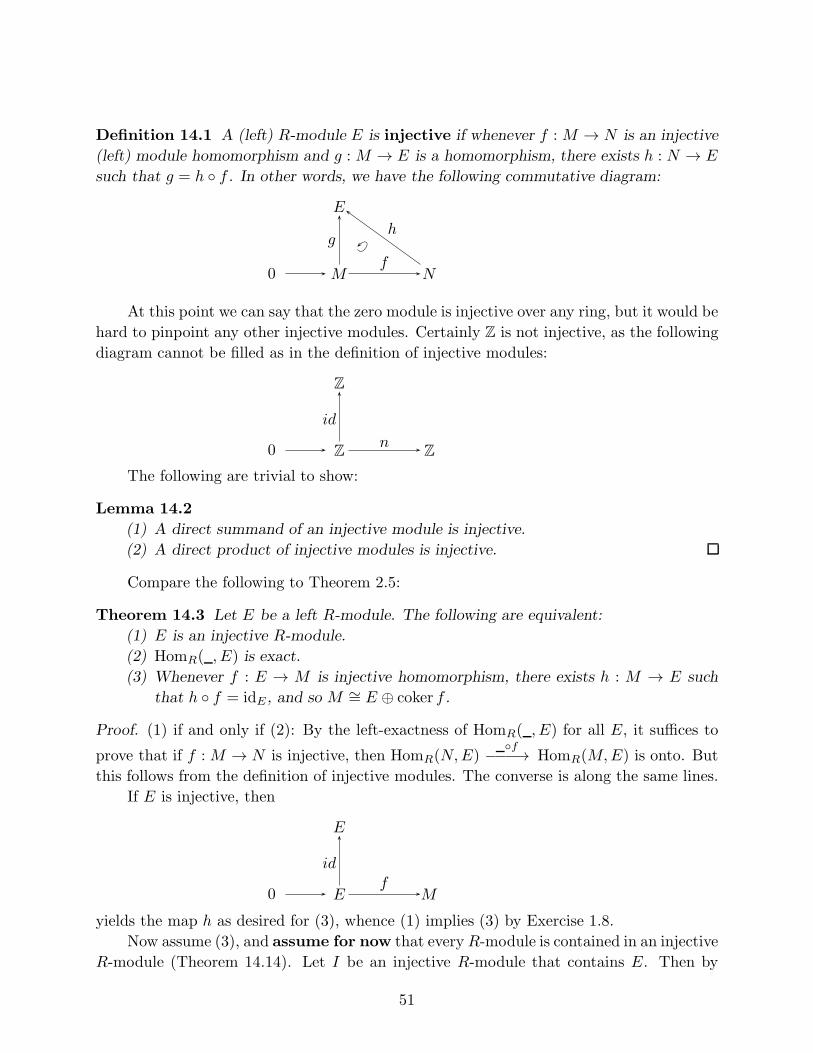
Definition 14.1 A (left) R-module E is injective if whenever f :M → N is an injective
(left) module homomorphism and g :M → E is a homomorphism, there exists h : N → E
such that g = h ◦ f . In other words, we have the following commutative diagram:
E
M N0f
gh
At this point we can say that the zero module is injective over any ring, but it would be
hard to pinpoint any other injective modules. Certainly Z is not injective, as the following
diagram cannot be filled as in the definition of injective modules:
Z
Z Z0n
id
The following are trivial to show:
Lemma 14.2
(1) A direct summand of an injective module is injective.
(2) A direct product of injective modules is injective.
Compare the following to Theorem 2.5:
Theorem 14.3 Let E be a left R-module. The following are equivalent:
(1) E is an injective R-module.
(2) HomR( , E) is exact.
(3) Whenever f : E → M is injective homomorphism, there exists h : M → E such
that h ◦ f = idE , and so M ∼= E ⊕ coker f .
Proof. (1) if and only if (2): By the left-exactness of HomR( , E) for all E, it suffices to
prove that if f :M → N is injective, then HomR(N,E)◦f−−−→ HomR(M,E) is onto. But
this follows from the definition of injective modules. The converse is along the same lines.
If E is injective, then
E
E M0f
id
yields the map h as desired for (3), whence (1) implies (3) by Exercise 1.8.
Now assume (3), and assume for now that every R-module is contained in an injective
R-module (Theorem 14.14). Let I be an injective R-module that contains E. Then by
51
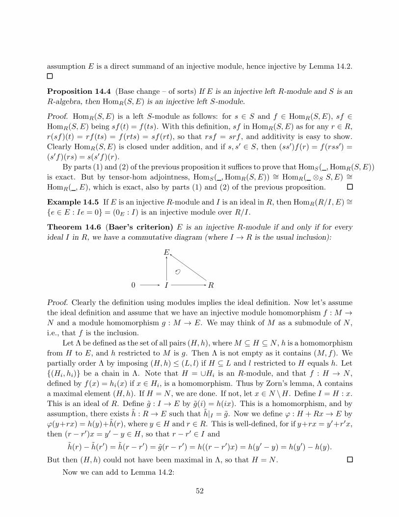
assumption E is a direct summand of an injective module, hence injective by Lemma 14.2.
Proposition 14.4 (Base change – of sorts) If E is an injective left R-module and S is an
R-algebra, then HomR(S,E) is an injective left S-module.
Proof. HomR(S,E) is a left S-module as follows: for s ∈ S and f ∈ HomR(S,E), sf ∈HomR(S,E) being sf(t) = f(ts). With this definition, sf in HomR(S,E) as for any r ∈ R,r(sf)(t) = rf(ts) = f(rts) = sf(rt), so that rsf = srf , and additivity is easy to show.
Clearly HomR(S,E) is closed under addition, and if s, s′ ∈ S, then (ss′)f(r) = f(rss′) =(s′f)(rs) = s(s′f)(r).
By parts (1) and (2) of the previous proposition it suffices to prove that HomS( ,HomR(S,E))
is exact. But by tensor-hom adjointness, HomS( ,HomR(S,E)) ∼= HomR( ⊗S S,E) ∼=HomR( , E), which is exact, also by parts (1) and (2) of the previous proposition.
Example 14.5 If E is an injective R-module and I is an ideal in R, then HomR(R/I, E) ∼={e ∈ E : Ie = 0} = (0E : I) is an injective module over R/I .
Theorem 14.6 (Baer’s criterion) E is an injective R-module if and only if for every
ideal I in R, we have a commutative diagram (where I → R is the usual inclusion):
E
I R0
Proof. Clearly the definition using modules implies the ideal definition. Now let’s assume
the ideal definition and assume that we have an injective module homomorphism f :M →N and a module homomorphism g : M → E. We may think of M as a submodule of N ,
i.e., that f is the inclusion.
Let Λ be defined as the set of all pairs (H, h), whereM ⊆ H ⊆ N , h is a homomorphism
from H to E, and h restricted to M is g. Then Λ is not empty as it contains (M, f). We
partially order Λ by imposing (H, h) ≤ (L, l) if H ⊆ L and l restricted to H equals h. Let
{(Hi, hi)} be a chain in Λ. Note that H = ∪Hi is an R-module, and that f : H → N ,
defined by f(x) = hi(x) if x ∈ Hi, is a homomorphism. Thus by Zorn’s lemma, Λ contains
a maximal element (H, h). If H = N , we are done. If not, let x ∈ N \H. Define I = H : x.
This is an ideal of R. Define g : I → E by g(i) = h(ix). This is a homomorphism, and by
assumption, there exists h : R → E such that h|I = g. Now we define ϕ : H +Rx→ E by
ϕ(y+rx) = h(y)+h(r), where y ∈ H and r ∈ R. This is well-defined, for if y+rx = y′+r′x,then (r − r′)x = y′ − y ∈ H, so that r − r′ ∈ I and
h(r)− h(r′) = h(r − r′) = g(r − r′) = h((r − r′)x) = h(y′ − y) = h(y′)− h(y).
But then (H, h) could not have been maximal in Λ, so that H = N .
Now we can add to Lemma 14.2:
52
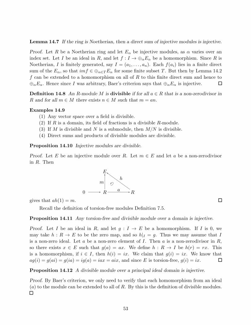
Lemma 14.7 If the ring is Noetherian, then a direct sum of injective modules is injective.
Proof. Let R be a Noetherian ring and let Eα be injective modules, as α varies over an
index set. Let I be an ideal in R, and let f : I → ⊕αEα be a homomorphism. Since R is
Noetherian, I is finitely generated, say I = (a1, . . . , an). Each f(ai) lies in a finite direct
sum of the Eα, so that imf ∈ ⊕α∈TEα for some finite subset T . But then by Lemma 14.2
f can be extended to a homomorphism on all of R to this finite direct sum and hence to
⊕αEα. Hence since I was arbitrary, Baer’s criterion says that ⊕αEα is injective.
Definition 14.8 An R-module M is divisible if for all a ∈ R that is a non-zerodivisor in
R and for all m ∈M there exists n ∈M such that m = an.
Examples 14.9
(1) Any vector space over a field is divisible.
(2) If R is a domain, its field of fractions is a divisible R-module.
(3) If M is divisible and N is a submodule, then M/N is divisible.
(4) Direct sums and products of divisible modules are divisible.
Proposition 14.10 Injective modules are divisible.
Proof. Let E be an injective module over R. Let m ∈ E and let a be a non-zerodivisor
in R. Then
E
R R0a
mh
gives that ah(1) = m.
Recall the definition of torsion-free modules Definition 7.5.
Proposition 14.11 Any torsion-free and divisible module over a domain is injective.
Proof. Let I be an ideal in R, and let g : I → E be a homomorphism. If I is 0, we
may take h : R → E to be the zero map, and so h|I = g. Thus we may assume that I
is a non-zero ideal. Let a be a non-zero element of I . Then a is a non-zerodivisor in R,
so there exists x ∈ E such that g(a) = ax. We define h : R → I be h(r) = rx. This
is a homomorphism, if i ∈ I , then h(i) = ix. We claim that g(i) = ix. We know that
ag(i) = g(ai) = g(ia) = ig(a) = iax = aix, and since E is torsion-free, g(i) = ix.
Proposition 14.12 A divisible module over a principal ideal domain is injective.
Proof. By Baer’s criterion, we only need to verify that each homomorphism from an ideal
(a) to the module can be extended to all of R. By this is the definition of divisible modules.
53
Examples 14.13
(1) Every field is an injective module over itself.
(2) If R is a principal ideal domain, then its field of fractions is an injective R-module.
Theorem 14.14 Every (left) module over a ring (with identity) embeds in an injective
module.
Proof. Let R be a ring and M an R-module.
First let R = Z. We can write M ∼= (⊕αZ)/H for some index set of α and for some
submodule H of ⊕αZ. Then M ⊆ (⊕αQ)/H, and the latter is divisible, hence injective.
Now let R be any ring. We have a canonical map Z → R. Then M can be also
considered as a Z-module, and as such it is embedded in an injective Z-module EZ . By
Proposition 14.4, E = HomZ(R,EZ) is a left injective R-module. Define f : M → E
as multiplication µm by m, i.e., by f(m)(r) = µm(r) = rm (here, we use that M is a
subset of EZ). Then f is certainly additive, and it is an R-module homomorphism (refer
to Proposition 14.4 for the R-module structure of E), as for any s ∈ R and any m ∈ M ,
f(sm)(r) = µsm(r) = rsm = (sµm)(r) = (sf)(r). Furthermore, f is injective, because if
rm = 0 for all r ∈ R, then m = 0. Thus M embeds in E as an R-module.
Note that this finishes the proof of Theorem 14.3.
15 Injective resolutions
Theorem 14.14 that we just proved shows that every module has an injective resolution,
where the definition is as follows:
Definition 15.1 An injective resolution of an R-module M is a cocomplex of injective
modules
0 → I0 → I1 → I2 → · · ·
such that 0 → M → I0 → I1 → I2 → · · · is exact. As noted before, and analogously
with the projective resolutions, for expediency in writing, when no confusion can arise,
0 →M → I0 → I1 → I2 → · · · is also sometimes called an injective resolution of M .
Example 15.2 Let R be a principal ideal domain, and let K be its field of fractions. Then
0 → R → K → K/R→ 0 is a finite injective resolution of R.
54
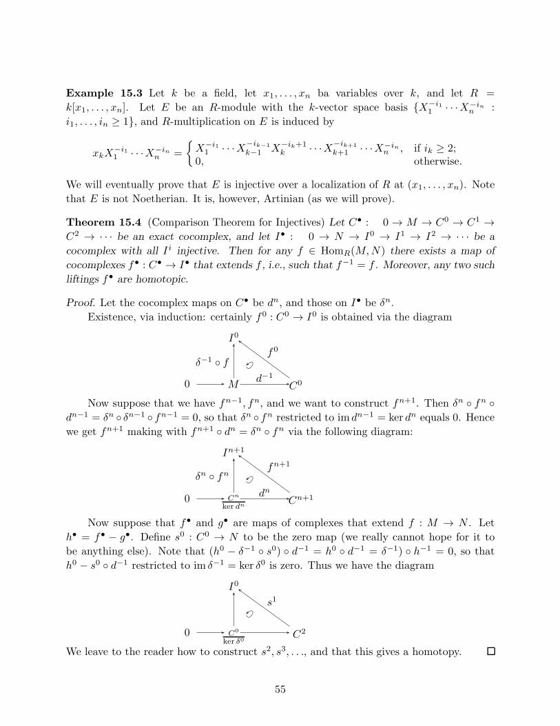
Example 15.3 Let k be a field, let x1, . . . , xn ba variables over k, and let R =
k[x1, . . . , xn]. Let E be an R-module with the k-vector space basis {X−i11 · · ·X−inn :
i1, . . . , in ≥ 1}, and R-multiplication on E is induced by
xkX−i11 · · ·X−inn =
{X−i11 · · ·X−ik−1
k−1 X−ik+1k · · ·X−ik+1
k+1 · · ·X−inn , if ik ≥ 2;0, otherwise.
We will eventually prove that E is injective over a localization of R at (x1, . . . , xn). Note
that E is not Noetherian. It is, however, Artinian (as we will prove).
Theorem 15.4 (Comparison Theorem for Injectives) Let C• : 0 → M → C0 → C1 →C2 → · · · be an exact cocomplex, and let I• : 0 → N → I0 → I1 → I2 → · · · be a
cocomplex with all I i injective. Then for any f ∈ HomR(M,N) there exists a map of
cocomplexes f• : C• → I• that extends f , i.e., such that f−1 = f . Moreover, any two such
liftings f• are homotopic.
Proof. Let the cocomplex maps on C• be dn, and those on I• be δn.Existence, via induction: certainly f0 : C0 → I0 is obtained via the diagram
I0
M C00d−1
δ−1 ◦ ff0
Now suppose that we have fn−1, fn, and we want to construct fn+1. Then δn ◦ fn ◦dn−1 = δn ◦ δn−1 ◦ fn−1 = 0, so that δn ◦ fn restricted to im dn−1 = ker dn equals 0. Hence
we get fn+1 making with fn+1 ◦ dn = δn ◦ fn via the following diagram:
In+1
Cn
ker dnCn+10
dnδn ◦ fn
fn+1
Now suppose that f• and g• are maps of complexes that extend f : M → N . Let
h• = f• − g•. Define s0 : C0 → N to be the zero map (we really cannot hope for it to
be anything else). Note that (h0 − δ−1 ◦ s0) ◦ d−1 = h0 ◦ d−1 = δ−1) ◦ h−1 = 0, so that
h0 − s0 ◦ d−1 restricted to im δ−1 = ker δ0 is zero. Thus we have the diagram
I0
C0
ker δ0C20
s1
We leave to the reader how to construct s2, s3, . . ., and that this gives a homotopy.
55
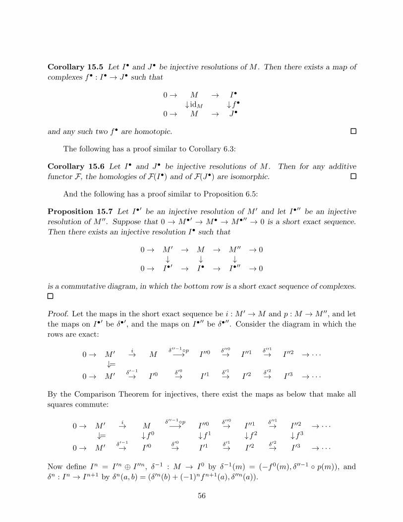
Corollary 15.5 Let I• and J• be injective resolutions of M . Then there exists a map of
complexes f• : I• → J• such that
0 → M → I•
↓ idM ↓f•0 → M → J•
and any such two f• are homotopic.
The following has a proof similar to Corollary 6.3:
Corollary 15.6 Let I• and J• be injective resolutions of M . Then for any additive
functor F, the homologies of F(I•) and of F(J•) are isomorphic.
And the following has a proof similar to Proposition 6.5:
Proposition 15.7 Let I•′ be an injective resolution of M ′ and let I•′′ be an injective
resolution of M ′′. Suppose that 0 → M•′ → M• → M•′′ → 0 is a short exact sequence.
Then there exists an injective resolution I• such that
0 → M ′ → M → M ′′ → 0↓ ↓ ↓
0 → I•′ → I• → I•′′ → 0
is a commutative diagram, in which the bottom row is a short exact sequence of complexes.
Proof. Let the maps in the short exact sequence be i :M ′ →M and p :M →M ′′, and let
the maps on I•′ be δ•′, and the maps on I•′′ be δ•′′. Consider the diagram in which the
rows are exact:
0 → M ′i→ M
δ′′−1◦p−→ I ′′0δ′′0→ I ′′1
δ′′1→ I ′′2 → · · ·↓=
0 → M ′δ′−1
→ I ′0δ′0→ I ′1
δ′1→ I ′2δ′2→ I ′3 → · · ·
By the Comparison Theorem for injectives, there exist the maps as below that make all
squares commute:
0 → M ′i→ M
δ′′−1◦p−→ I ′′0δ′′0→ I ′′1
δ′′1→ I ′′2 → · · ·↓= ↓f0 ↓f1 ↓f2 ↓f3
0 → M ′δ′−1
→ I ′0δ′0→ I ′1
δ′1→ I ′2δ′2→ I ′3 → · · ·
Now define In = I ′n ⊕ I ′′n, δ−1 : M → I0 by δ−1(m) = (−f0(m), δ′′−1 ◦ p(m)), and
δn : In → In+1 by δn(a, b) = (δ′n(b) + (−1)nfn+1(a), δ′′n(a)).
56
This works. Namely, let m ∈ ker δ−1. Then δ′′−1◦p(m) = 0, so that p(m) = 0, whence
m = i(m′) for some m′ ∈ M ′. Also, 0 = f0(m) = f0 ◦ i(m′) = δ′−1(m′), so that m′ = 0
and so m = i(m′) = 0. So δ−1 is injective.
Exactness at I0: δ0 ◦ δ−1(m) = δ0(−f0(m), δ′′−1 ◦ p(m)) = (−δ′0 ◦ f0(m)+ f1 ◦ δ′′−1 ◦p(m), δ′′0 ◦ δ′′−1 ◦ p(m)) = 0, so that im δ−1 ⊆ ker δ0. If (a, b) ∈ ker δ0, then δ′′0(b) = 0
and δ′0(a) + f1(b) = 0. Thus b = δ′′−1(m′′) for some m ∈ M ′′, and even b = δ′′−1 ◦ p(m)
for some m ∈ M , and δ′0(a) = −f1(b) = −f1 ◦ δ′′−1 ◦ p(m) = −δ′0 ◦ f0(m), whence
a + f0(m) ∈ ker δ′0 = δ′−1M ′, so that a + f0(m) = δ′−1m′ for some m′ ∈ M . Then
δ−1(m − i(m′)) = (−f0(m − i(m′)), δ′′−1 ◦ p(m + i(m′))) = (−f0(m) + f0 ◦ i(m′), δ′′−1 ◦p(m)) = (−δ′−1m′ + a+ δ′−1(m′), b) = (a, b), which proves that im δ−1 = ker δ0.
For n ≥ 0, δn+1 ◦ δn(a, b) = δn+1(δ′n(b) + (−1)nfn+1(a), δ′′n(a)) = (δ′n+1 ◦(δ′n(b) + (−1)nfn+1(a) + (−1)n+1fn+2 ◦ δ′′n(a), δ′′n+1 ◦ δ′′n(a))) = 0. This proves
that im δn ⊆ ker δn+1. Now let (a, b) ∈ ker δn+1. Then δ′′n+1(b) = 0 and δ′n+1(a) +
(−1)n+1fn+2(b) = 0. It follows that b = δ′′n(c) for some c ∈ I ′′n. Then δ′n+1(a) =
(−1)nfn+2 ◦ δ′′n(c) = (−1)nδ′n+1 ◦ fn+1(c), so that a− (−1)nfn+1(c) ∈ ker δ′n+1 = im δ′n,whence a− (−1)nfn+1(c) = δ′n(d) for some d ∈ I ′n. Thus
δn(d, c) = (δ′n(d)+(−1)nfn+1(c), δ′′n(c)) = (a− (−1)nfn+1(c)+(−1)nfn+1(c), b) = (a, b),
which proves that ker δn+1 = im δn for all n ≥ 0.
We leave it to the reader to verify that this makes a short exact sequence of injective
resolutions.
16 A definition of Ext using injective resolutions
LetM,N be R-modules, and let I• : 0 → I0 → I1 → I2 · · · be an injective resolution
of M . We define
Extn
R(M,N) = Hn(HomR(M, I•)).
With the manipulations of injective resolutions in the previous section we can fairly
quickly develop some main properties of Ext:
1. Independence of the resolution. The definition of Extn
R( , N) is independent of the
injective resolution I• of N . This follows from Corollary 15.6.
2. Ext has no terms of negative degree. Extn
R( , N) = 0 if n < 0. This follows as I•
has only zero modules in negative positions.
3. Ext0. Ext
0
R(M,N) ∼= HomR(M,N). Proof: By assumption 0 → N → I0 → I1 is exact,
and as Hom(M, ) is left-exact, 0 → HomR(M,N) → HomR(I0, N) → HomR(I
1, N)
is exact as well. Thus Ext0
R(M,N) = H0(HomR(M, I•)) = ker(HomR(I0, N) →
HomR(I1, N)) = HomR(M,N).
57
4. What if M is projective? If M is projective, then Extn
R(M,N) = 0 for all n ≥ 1.
This follows as In−1 → In → In+1 is exact, and so as M is projective, HomR(M,Pn−1) →HomR(M,Pn) → HomR(M,Pn+1) is exact as well, giving that the nth cohomology of
HomR(M, I•) is 0 if n > 0.
5. What if N is injective? If N is injective, then Extn
R(M,N) = 0 for all n ≥ 1. This
is clear as in that case we may take I0 = N and all other In to be 0.
6. Ext on short exact sequences. If 0 → N ′ → N → N ′′ → 0 is a short exact sequence
of modules, then for any module M , there is a long exact sequence
· · · → Extn−1R (M,N ′′) → ExtnR(M,N ′) → ExtnR(M,N) → ExtnR(M,N ′′) → Extn+1R (M,N ′) → · · · .
The proof goes as follows. Let I•′ be an injective resolution of N ′, and let I•′′ be an
injective resolution of N ′′. Then by Proposition 15.7 there exists an injective resolution I•
of N such that0 → N ′ → N → N ′′ → 0
↓ ↓ ↓0 → I•′ → I• → I•′′ → 0
is a commutative diagram in which the rows are exact. In particular, we have a short exact
sequence 0 → I•′ → I• → I•′′ → 0, and since this is a split exact sequence, it follows that
0 → HomR(M, I•′′) → HomR(M, I•) → HomR(M, I•′) → 0 is still a short exact sequence
of complexes. The rest follows from Theorem 4.4.
Exercise 16.1 Let x ∈ R and suppose that 0 → Nx→ N → N/xN → 0 is a short exact
sequence. Prove that the maps ExtnR(M,N) → ExtnR(M,N) in the long exact sequence
above are also multiplications by x.
Exercise 16.2 Prove that for anyR-modulesM andN , annM+annN ⊆ ann Extn
R(M,N).
Exercise 16.3 Let 0 → N → I0 → I1 → · · · → In−1 → Nn → 0 be exact, where all Ij
are injective. Prove that for all i ≥ 1, Exti
R(M,Nn) ∼= Exti+n
R (M,N).
17 A definition of Ext using projective resolutions
Let M,N be R-modules, and let P• : · · · → P2 → P1 → P0 → 0 be a projective
resolution of M . We define
ExtnR(M,N) = Hn(HomR(P•, N)).
With all the general manipulations of complexes we can fairly quickly develop some
main properties of Ext:
1. Independence of the resolution. The definition of ExtnR(M, ) is independent of the
projective resolution P• of M . This follows from Corollary 6.3.
58
2. Ext has no terms of negative degree. ExtnR(M, ) = 0 if n < 0. This follows as P•has only zero modules in negative positions.
3. Ext0. Ext0R(M,N) ∼= HomR(M,N). Proof: By assumption P1 → P0 → M → 0 is ex-
act, and as Hom( , N) is left-exact, 0 → HomR(M,N) → HomR(P0, N) → HomR(P1, N)
is exact as well. Thus Ext0R(M,N) = H0(HomR(P•, N)) = ker(HomR(P0, N) →HomR(P1, N)) = HomR(M,N).
4. What if M is projective? If M is projective, then ExtnR(M,N) = 0 for all n ≥ 1.
This is clear as in that case we may take P0 =M and all other Pn to be 0.
5. What if N is injective? If N is injective, then ExtnR(M,N) = 0 for all n ≥ 1. This
follows as Pn+1 → Pn → Pn−1 is exact, and so as N is injective, HomR(Pn−1, N) →HomR(Pn, N) → HomR(Pn+1, N) is exact as well, giving that the nth cohomology of
HomR(P•, N) is 0 if n > 0.
6. Ext on short exact sequences. If 0 → M ′ → M → M ′′ → 0 is a short exact se-
quence of modules, then for any module N , there is a long exact sequence
· · · → Extn−1R (M ′, N) → ExtnR(M′′, N) → ExtnR(M,N) → ExtnR(M
′, N) → Extn+1R (M ′′, N) → · · · .
The proof goes as follows. Let P•′ be a projective resolution of M ′, and let P•
′′ be a
projective resolution of M ′′. Then by Proposition 6.5 there exists a projective resolution
P• of M such that0 → P•
′ → P• → P•′′ → 0
↓ ↓ ↓0 → M ′ → M → M ′′ → 0
is a commutative diagram in which the rows are exact. In particular, we have a short exact
sequence 0 → P•′ → P• → P•
′′ → 0, and since this is a split exact sequence, it follows that
0 → HomR(P•′′, N) → HomR(P•, N) → HomR(P•
′, N) → 0 is still a short exact sequence
of complexes. The rest follows from Theorem 4.4.
7. Ext and annihilators. For any M,N and n, annM + annN ⊆ ann ExtnR(M,N).
Proof: Since ExtnR(M,N) is a quotient of a submodule of HomR(Pn, N), it is clear that
annN annihilates all Exts. Now let x ∈ annM . Then multiplication by x on M , which
is the same as multiplication by 0 on M , has two lifts µx and µ0 on P•, and by the
Comparison Theorem Theorem 4.9, the two maps are homotopic. Thus HomR(µx, N) and
0 are homotopic on HomR(P•, N), whence by Proposition 4.7, HomR(µx, N)∗ = 0. In other
words, multiplication by x on HomR(P•, N) is zero.
8. Ext on syzygies. LetMn be an nth syzygy ofM , i.e., 0 →Mn → Pn−1 → · · · → P1 →P0 →M → 0 is exact for some projective modules Pi. Then for all i ≥ 1, ExtiR(Mn, N) ∼=Exti+n
R (M,N). This follows from the definition of Ext (and from the independence on the
projective resolution).
9. Ext for finitely generated modules over Noetherian rings. If R is Noetherian
and M and N are finitely generated R-modules, then ExtnR(M,N) is a finitely generated
59
R-module for all n. To prove this, we may choose P• such that all Pn are finitely generated
(since submodules of finitely generated modules are finitely generated). Then HomR(Pn, N)
is finitely generated, whence so is ExtnR(M,N).
Exercise 17.1 Let x ∈ R and suppose that 0 →Mx→ M →M/xM → 0 is a short exact
sequence. Prove that the maps ExtnR(M,N) → ExtnR(M,N) in the long exact sequence are
also multiplications by x.
18 The two definitions of Ext are isomorphic
Theorem 18.1 Let R be a commutative ring and let M and N be R-modules. Then for
all n, ExtRn (M,N) ∼= ExtR
n (M,N).
Proof. Let P• be a projective resolution of M and let I• be an injective resolution of N .
Let M1, N1 be defined so that 0 → M1 → P0 → M → 0 and 0 → N → I0 → N1 → 0
are exact. By applying HomR we get the following commutative diagram whose rows and
columns are exact:
0 0 0↓ ↓ ↓
0 → Hom(M,N) → Hom(P0, N) → Hom(M1, N)↓ ↓ ↓
0 → Hom(M, I0) → Hom(P0, I0) → Hom(M1, I
0) → 0↓α ↓β ↓γ
0 → Hom(M,N1) → Hom(P0, N1) → Hom(M1, N1)↓ ↓
Ext1
R(M,N) 0↓
Ext1
R(M, I0) = 0
By the Snake Lemma (Lemma 1.5), 0 → kerα → ker β → ker γ → cokerα → cokerβ is
exact, or in other words,
0 → HomR(M,N) → HomR(P0, N) → HomR(M1, N) → Ext1
R(M,N) → 0
is exact. Note that the maps between the Hom modules above are the natural maps. But
we also have that
0 → HomR(M,N) → HomR(P0, N) → HomR(M1, N) → Ext1R(M,N) → Ext1R(P0, N) = 0
is exact with the natural maps on the Hom modules, which proves that for all R-modules
M and N , Ext1R(M,N) = Ext1
R(M,N).
60
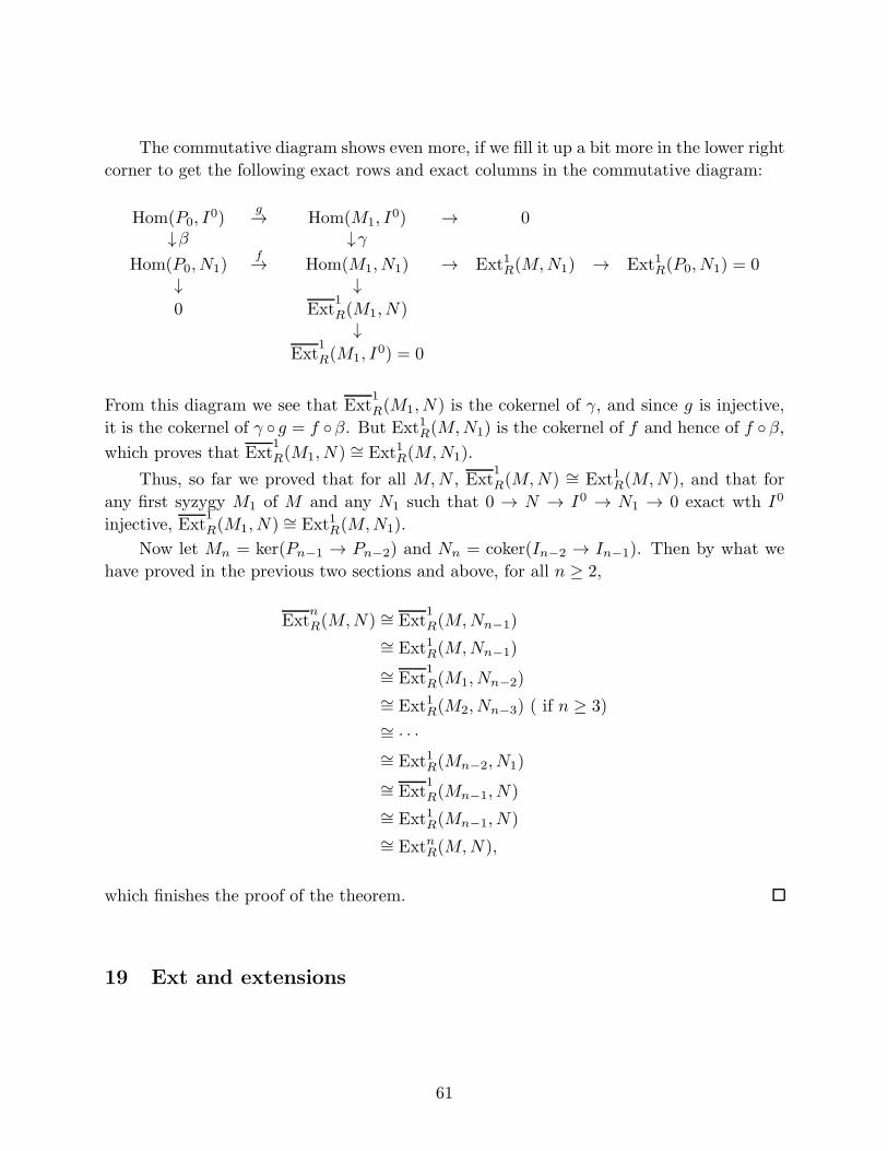
The commutative diagram shows even more, if we fill it up a bit more in the lower right
corner to get the following exact rows and exact columns in the commutative diagram:
Hom(P0, I0)
g→ Hom(M1, I0) → 0
↓β ↓γHom(P0, N1)
f→ Hom(M1, N1) → Ext1R(M,N1) → Ext1R(P0, N1) = 0↓ ↓0 Ext
1
R(M1, N)↓
Ext1
R(M1, I0) = 0
From this diagram we see that Ext1
R(M1, N) is the cokernel of γ, and since g is injective,
it is the cokernel of γ ◦ g = f ◦β. But Ext1R(M,N1) is the cokernel of f and hence of f ◦β,which proves that Ext
1
R(M1, N) ∼= Ext1R(M,N1).
Thus, so far we proved that for all M,N , Ext1
R(M,N) ∼= Ext1R(M,N), and that for
any first syzygy M1 of M and any N1 such that 0 → N → I0 → N1 → 0 exact wth I0
injective, Ext1
R(M1, N) ∼= Ext1R(M,N1).
Now let Mn = ker(Pn−1 → Pn−2) and Nn = coker(In−2 → In−1). Then by what we
have proved in the previous two sections and above, for all n ≥ 2,
Extn
R(M,N) ∼= Ext1
R(M,Nn−1)
∼= Ext1R(M,Nn−1)
∼= Ext1
R(M1, Nn−2)
∼= Ext1R(M2, Nn−3) ( if n ≥ 3)
∼= · · ·∼= Ext1R(Mn−2, N1)
∼= Ext1
R(Mn−1, N)
∼= Ext1R(Mn−1, N)
∼= ExtnR(M,N),
which finishes the proof of the theorem.
19 Ext and extensions
61
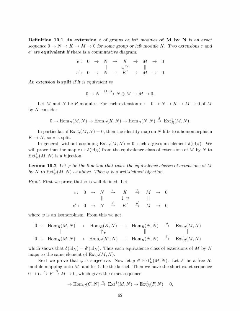
Definition 19.1 An extension e of groups or left modules of M by N is an exact
sequence 0 → N → K → M → 0 for some group or left module K. Two extensions e and
e′ are equivalent if there is a commutative diagram:
e : 0 → N → K → M → 0|| ↓ ∼= ||
e′ : 0 → N → K′ → M → 0
An extension is split if it is equivalent to
0 → N(1,0)−−−→ N ⊕M →M → 0.
Let M and N be R-modules. For each extension e : 0 → N → K → M → 0 of M
by N consider
0 → HomR(M,N) → HomR(K,N) → HomR(N,N)δ→ Ext1R(M,N).
In particular, if Ext1R(M,N) = 0, then the identity map on N lifts to a homomorphism
K → N , so e is split.
In general, without assuming Ext1R(M,N) = 0, each e gives an element δ(idN ). We
will prove that the map e 7→ δ(idN ) from the equivalence class of extensions of M by N to
Ext1R(M,N) is a bijection.
Lemma 19.2 Let ϕ be the function that takes the equivalence classes of extensions of M
by N to Ext1R(M,N) as above. Then ϕ is a well-defined bijection.
Proof. First we prove that ϕ is well-defined. Let
e : 0 → Ni→ K
p→ M → 0|| ↓ ϕ ||
e′ : 0 → Ni′→ K′
p′
→ M → 0
where ϕ is an isomorphism. From this we get
0 → HomR(M,N) → HomR(K,N) → HomR(N,N)δ→ Ext1R(M,N)
|| ↑ϕ || ||0 → HomR(M,N) → HomR(K
′, N) → HomR(N,N)δ′→ Ext1R(M,N)
which shows that δ(idN ) = δ′(idN ). Thus each equivalence class of extensions of M by N
maps to the same element of Ext1R(M,N).
Next we prove that ϕ is surjective. Now let g ∈ Ext1R(M,N). Let F be a free R-
module mapping onto M , and let C be the kernel. Then we have the short exact sequence
0 → Cα→ F
β→ M → 0, which gives the exact sequence
→ HomR(C,N)γ→ Ext1(M,N) → Ext1R(F,N) = 0,
62
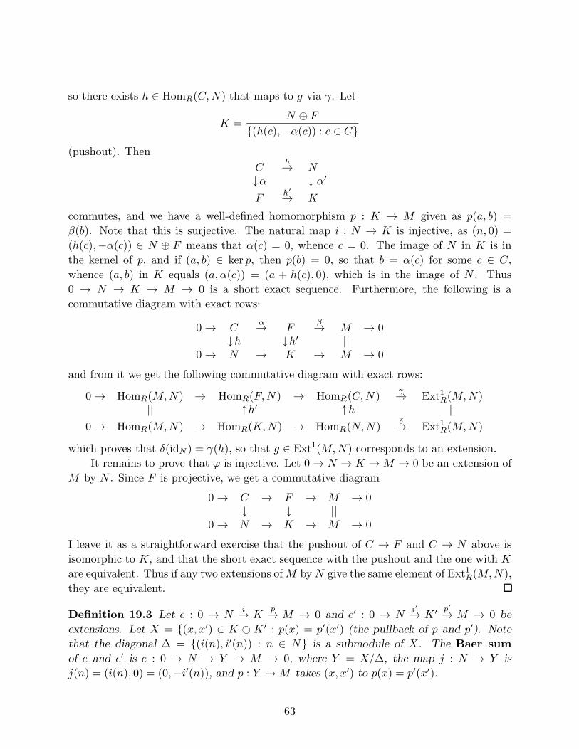
so there exists h ∈ HomR(C,N) that maps to g via γ. Let
K =N ⊕ F
{(h(c),−α(c)) : c ∈ C}(pushout). Then
Ch→ N
↓α ↓ α′F
h′
→ K
commutes, and we have a well-defined homomorphism p : K → M given as p(a, b) =
β(b). Note that this is surjective. The natural map i : N → K is injective, as (n, 0) =
(h(c),−α(c)) ∈ N ⊕ F means that α(c) = 0, whence c = 0. The image of N in K is in
the kernel of p, and if (a, b) ∈ ker p, then p(b) = 0, so that b = α(c) for some c ∈ C,
whence (a, b) in K equals (a, α(c)) = (a + h(c), 0), which is in the image of N . Thus
0 → N → K → M → 0 is a short exact sequence. Furthermore, the following is a
commutative diagram with exact rows:
0 → Cα→ F
β→ M → 0↓h ↓h′ ||
0 → N → K → M → 0
and from it we get the following commutative diagram with exact rows:
0 → HomR(M,N) → HomR(F,N) → HomR(C,N)γ→ Ext1R(M,N)
|| ↑h′ ↑h ||0 → HomR(M,N) → HomR(K,N) → HomR(N,N)
δ→ Ext1R(M,N)
which proves that δ(idN ) = γ(h), so that g ∈ Ext1(M,N) corresponds to an extension.
It remains to prove that ϕ is injective. Let 0 → N → K →M → 0 be an extension of
M by N . Since F is projective, we get a commutative diagram
0 → C → F → M → 0↓ ↓ ||
0 → N → K → M → 0
I leave it as a straightforward exercise that the pushout of C → F and C → N above is
isomorphic to K, and that the short exact sequence with the pushout and the one with K
are equivalent. Thus if any two extensions ofM byN give the same element of Ext1R(M,N),
they are equivalent.
Definition 19.3 Let e : 0 → Ni→ K
p→ M → 0 and e′ : 0 → Ni′→ K′
p′
→ M → 0 be
extensions. Let X = {(x, x′) ∈ K ⊕ K′ : p(x) = p′(x′) (the pullback of p and p′). Note
that the diagonal ∆ = {(i(n), i′(n)) : n ∈ N} is a submodule of X. The Baer sum
of e and e′ is e : 0 → N → Y → M → 0, where Y = X/∆, the map j : N → Y is
j(n) = (i(n), 0) = (0,−i′(n)), and p : Y →M takes (x, x′) to p(x) = p′(x′).
63
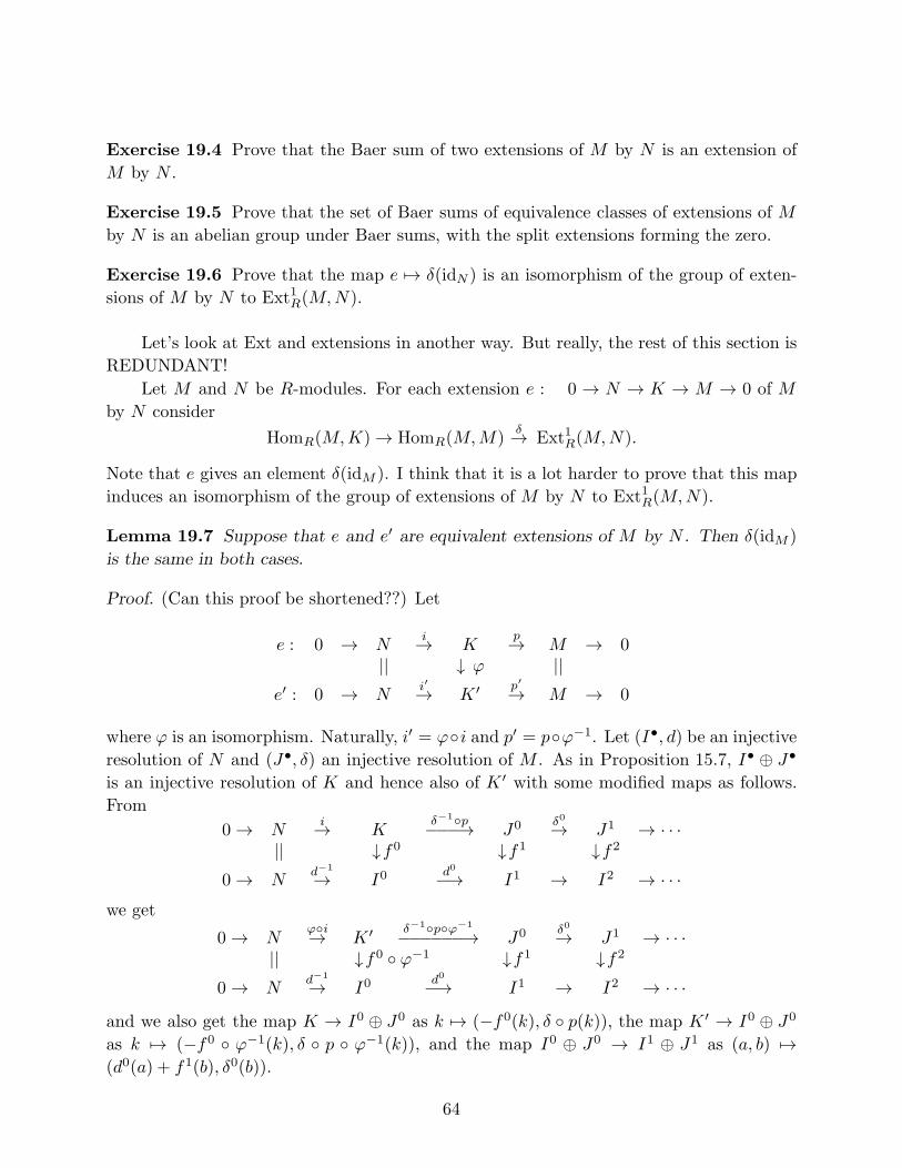
Exercise 19.4 Prove that the Baer sum of two extensions of M by N is an extension of
M by N .
Exercise 19.5 Prove that the set of Baer sums of equivalence classes of extensions of M
by N is an abelian group under Baer sums, with the split extensions forming the zero.
Exercise 19.6 Prove that the map e 7→ δ(idN ) is an isomorphism of the group of exten-
sions of M by N to Ext1R(M,N).
Let’s look at Ext and extensions in another way. But really, the rest of this section is
REDUNDANT!
Let M and N be R-modules. For each extension e : 0 → N → K → M → 0 of M
by N consider
HomR(M,K) → HomR(M,M)δ→ Ext1R(M,N).
Note that e gives an element δ(idM ). I think that it is a lot harder to prove that this map
induces an isomorphism of the group of extensions of M by N to Ext1R(M,N).
Lemma 19.7 Suppose that e and e′ are equivalent extensions of M by N . Then δ(idM )
is the same in both cases.
Proof. (Can this proof be shortened??) Let
e : 0 → Ni→ K
p→ M → 0|| ↓ ϕ ||
e′ : 0 → Ni′→ K′
p′
→ M → 0
where ϕ is an isomorphism. Naturally, i′ = ϕ◦i and p′ = p◦ϕ−1. Let (I•, d) be an injective
resolution of N and (J•, δ) an injective resolution of M . As in Proposition 15.7, I• ⊕ J•
is an injective resolution of K and hence also of K′ with some modified maps as follows.
From
0 → Ni→ K
δ−1◦p−−−→ J0 δ0→ J1 → · · ·|| ↓f0 ↓f1 ↓f2
0 → Nd−1
→ I0d0
−→ I1 → I2 → · · ·we get
0 → Nϕ◦i→ K′
δ−1◦p◦ϕ−1
−−−−−−→ J0 δ0→ J1 → · · ·|| ↓f0 ◦ ϕ−1 ↓f1 ↓f2
0 → Nd−1
→ I0d0
−→ I1 → I2 → · · ·and we also get the map K → I0 ⊕ J0 as k 7→ (−f0(k), δ ◦ p(k)), the map K′ → I0 ⊕ J0
as k 7→ (−f0 ◦ ϕ−1(k), δ ◦ p ◦ ϕ−1(k)), and the map I0 ⊕ J0 → I1 ⊕ J1 as (a, b) 7→(d0(a) + f1(b), δ0(b)).
64
We get exact rows and columns in the following:
0 0 0↓ ↓ ↓
0 → HomR(M,N) → HomR(M,K) → HomR(M,M)↓ ↓ ↓
0 → HomR(M, I0) → HomR(M, I0 ⊕ J0) → HomR(M,J0) → 0↓ α ↓ β ↓ γ
0 → HomR(M, I1) → HomR(M, I1 ⊕ J1) → HomR(M,J1) → 0
We apply the Snake Lemma (on α, β, γ). Here idM ∈ HomR(M,M) ⊆ HomR(M,J0) is
in the kernel of γ, or more precisely, δ−1 ∈ HomR(M,J0) is in the kernel, and so maps
to cokerα as follows. First of all, δ−1 ∈ HomR(M,J0) is the image of (0, δ−1) : M →I0 ⊕ J0. The image of (0, δ−1) in HomR(M, I1 ⊕ J1) is (f1 ◦ δ−1, 0), and its preimage
in HomR(M, I1) is f1 ◦ δ−1. Let m ∈ M . Write m = p(k) for some k ∈ K. Then
d1 ◦ f1 ◦ δ−1(m) = d1 ◦ d0 ◦ f0(m) = 0, so that f1 ◦ δ−1 is in the kernel of the map
HomR(M, I1) → HomR(M, I2), or in other words, idM maps to the image of f1 ◦ δ−1 in
Ext1(M,N).
We have all the information to say what happens with the extension e′: idM maps to
the same element f1 ◦ δ−1 as the idM arising from the extension e.
Exercise 19.8 (Which I am not able to solve right now.) Now letM and N be R-modules,
let g ∈ Ext1R(M,N). Let F be a free R-module mapping onto M , and let C be the kernel.
Then the short exact sequence 0 → Cα→ F
β→ M → 0 gives the exact sequence
→ HomR(C,N)γ→ Ext1(M,N) → Ext1R(F,N) = 0,
so there exists h ∈ HomR(C,N) that maps onto g via γ. Let
K =N ⊕ F
{(h(c),−α(c)) : c ∈ C}
(pushout). Then
Ch→ N
↓α ↓ α′F
h′
→ K
commutes, and we have a well-defined homomorphism p : K → M given as p(a, b) =
β(b). Note that this is surjective. The natural map i : N → K is injective, as (n, 0) =
(h(c),−α(c)) ∈ N ⊕ F means that α(c) = 0, whence c = 0. The image of N in K is in
the kernel of p, and if (a, b) ∈ ker p, then p(b) = 0, so that b = α(c) for some c ∈ C,
whence (a, b) in K equals (a, α(c)) = (a + h(c), 0), which is in the image of N . Thus
0 → N → K → M → 0 is a short exact sequence. Show that this extension yields the
original g ∈ Ext1R(M,N).
65
20 Essential extensions
In this section we look more closely at the structure of injective modules.
Definition 20.1 An extension M ⊆ N of R-modules is said to be essential (over R) if
for every non-zero submodule K of N , K ∩M is non-zero.
Remark 20.2
(1) If R is a domain and K its field of fractions, then R ⊆ K is essential.
(2) If M ⊆ L and L ⊆ N are essential extensions of R-modules, then so is M ⊆ N .
(3) M ⊆ N is essential if and only if for all non-zero x ∈ N there exists r ∈ R such
that rx is a non-zero element of M .
(4) Let M ⊆ Lα ⊆ N be R-modules as α varies over some index set. If M ⊆ Lα is
essential for all α, then M ⊆ ∪Lα is essential (whenever the union is a module).
(Proof: previous part.)
(5) If M ⊆ N is essential and S is a multiplicatively closed subset of R such that
S−1M 6= 0, then S−1M ⊆ S−1N is essential over S−1R.
Lemma 20.3 Let M ⊆ N be an inclusion of R-modules. Then there exists a module L
between M and N such that M ⊆ L is essential, and L is a maximal submodule of N with
this property.
Proof. Zornify the set of all intermediate modules that are essential over M . The set is
non-empty as it contains M . By the last part of Remark 20.2, every chain has an upper
bound. Thus by Zorn’s lemma the existence conclusion follows.
Proposition 20.4 An R-module E is injective if and only if there does not exist a proper
essential extension of E.
Proof. Suppose that E is injective and that E ( N is an essential extension. By Theo-
rem 14.3, N ∼= E ⊕M for some non-zero module M , whence no non-zero multiple of a
non-zero element of M is in E, which gives a contradiction.
Now suppose that E has no proper essential extension. By Theorem 14.3 it suffices to
prove that any injective homomorphism f : E → M splits. Without loss of generality M
is different from E. By assumption for every x ∈ M \ E, Rx ∩E = 0. Let Λ be the set of
all submodules K of M such that K ∩E = 0. We just proved that Λ is not empty. We can
Zornify Λ, and (verify details) there exists a maximal element K in Λ. Since K ∩ E = 0,
we have that K +E = K ⊕E ⊆M , and that E injects into M/K.
We claim that E → M/K is essential: otherwise there exists a non-zero submodule
L/K of M/K such that E ∩ (L/K) = 0. But then E ∩ L ⊆ E ∩ K = 0, whence by
maximality of K, we have L = K.
But then by assumption E = M/K, i.e., (E +K)/K = M/K, so that E +K = M ,
so that E ⊕K =M , so E is a direct summand of M via inclusion.
66
Now we can make Lemma 20.3 more precise under an additional assumption:
Lemma 20.5 Let M ⊆ N be an inclusion of R-modules and suppose that N is injective.
Then there exists a submodule L of N that is maximal with respect to the property that
it is essential over M , and any such L is injective.
Proof. By Lemma 20.3 there exists a submodule L of N that is maximal among all
essential extensions of M in N . Suppose for contradiction that L is not injective. Then by
Proposition 20.4, L has a proper essential extension E (which is not necessarily a submodule
of N). Since N is injective, by definition we have
N
L E0
h
If ker h 6= 0, then since L → E is essential, there exists a non-zero element x ∈ L ∩ ker h,
which gives a contradiction to the commutative diagram since L embeds in N . Thus h is
injective. Hence M ⊆ L ⊆ E ⊆ N . By transitivity of essential extensions (Remark 20.2),
E is an essential extension of M . Thus by the maximality of L in E, L = E. So L has no
proper essential extensions, so by Proposition 20.4, L is injective.
Theorem 20.6 LetM be an R-module. Then there exists an overmodule that is injective
and essential over M . Any two such overmodules are isomorphic.
Proof. By Theorem 14.14 there exists an injective R-module N containing M , and
Lemma 20.5 finishes the proof of existence.
Suppose that E and E′ are injective modules that are essential over M . Then
E′
M E0
h
and h has to be injective as E is essential over M and M embeds in E′. Since h and E
are injective, it E must be a direct summand of E′, and since E′ is essential over M , the
complementary direct summand must be 0, so that E′ ∼= E.
Definition 20.7 The module constructed in the previous theorem (unique up to isomor-
phism) is called the injective hull or the injective envelope ofM . It is denoted ER(M).
67
Theorem 20.8 Let M ⊆ E be R-modules. The following are equivalent:
(1) E is a maximal essential extension of M .
(2) E is injective, M ⊆ E is essential.
(3) E ∼= ER(M).
(4) E is injective, and if M ⊆ E′ ⊆ E with E′ injective, then E′ = E.
Proof. Assume (1). Clearly M ⊆ E is essential. Let F be an essential extension of E.
Then by one of the remarks, F is an essential extension of M , and by the maximality
assumption in (1), E = F , so by Proposition 20.4, E is injective. This proves (2).
(2) and (3) are equivalent by definition.
Assume (2). Let E′ be an injective module such thatM ⊆ E′ ⊆ E. By Theorem 14.3,
E ∼= E′ ⊕ E′′ for some submodule E′′ of E. Then E′′ ∩M = 0, so by assumption (2),
E′′ = 0. This proves (4).
Assume (4). By Lemma 20.5 there exists a maximal essential extension E′ of M that
is contained in E, and such that E′ is injective. Hence by assumption (4), E′ = E, so E is
essential over M . Any essential extension of M that contains E would have to have E as
a direct summand as E is injective, but then by the essential property the complementary
direct summand would have to be 0. Thus (1) follows.
The following is now clear:
Corollary 20.9 If E is an injective R-module, then ER(E) = E.
Proposition 20.10 If M ⊆ N , then ER(M) embeds in ER(N).
Proof. In the diagram
ER(N)
M ER(M)0
h
the homomorphism h must be injective, for otherwise since M → ER(M) is essential, a
non-zero element of M maps to 0 in N ⊆ ER(N), which is a contradiction. This gives the
desired imbedding.
Definition 20.11 Note that in this section we proved that every R-module M has an
injective resolution 0 → I0 → I1 → I2 → · · ·, where I0 is an essential extension of M , I1 is
an essential extension of I0/M , and for all i ≥ 2, I i is an essential extension of the cokernel
of I i−2 → I i−1. Such an injective resolution is called a minimal injective resolution.
68
Proposition 20.12 Let (R,m) be a Noetherian ring and let M be an R-module. Prove
that HomR(R/m,M) ∼= HomR(R/m, ER(M)).
Proof. Define ϕ : HomR(R/m,M) → HomR(R/m, ER(M)) via the standard inclusion
M ⊆ ER(M). Clearly ϕ is injective. Now let f ∈ HomR(R/m, ER(M)). This f is
uniquely determined by f(1) ∈ ER(M). Since M → ER(M) is essential, if f(1) 6= 0 there
exists r ∈ R such that rf(1) is non-zero in M . If r ∈ m, then 0 = f(0) = f(r) = rf(1), so
necessarily r is a unit in R. But then the image of f is inM , so that HomR(R/m, ER(M)) ⊆HomR(R/m,M).
Theorem 20.13 Let I• be a minimal injective resolution of an R-module M . Then for
all P ∈ Spec (R) and all i ≥ 0, HomRP(RP /PRP , (I
i)P ) → HomRP(RP /PRP , (I
i+1)P ) is
the zero map.
Proof. By Exercise 20.14, (I•)P is an injective resolution of MP , and by Remark 20.2, it
is a minimal injective resolution of MP .
Let Qi be the kernel of I i → I i+1 (i.e., the cokernel of I i−2 → Ii−1). Then 0 →Qi → I i → I i+1 → I i+2 → · · · is exact. Since localization and Hom are left-exact (see
Exercise 1.7), it follows that
0 → HomRP(RP /PRP , Q
i)f→ HomRP
(RP /PRP , Ii)
g→ HomRP(RP /PRP , I
i+1)
is exact. Since I• is minimal, I i is an essential extension of Qi, so that by Proposition 20.12,
HomRP(RP /PRP , Q
i)f→ HomRP
(RP /PRP , Ii) is an isomorphism. Thus g is zero.
Exercise 20.14 Let M → L be an essential extension, let L → K be a homomorphism
such that the composition M → L→ K is injective. Prove that L→ K is injective.
Exercise 20.15 Prove that a localization of an injective module over a Noetherian ring is
injective.
Exercise 20.16 Let P and Q be prime ideals in a Noetherian ring R with Q 6⊆ P . Prove
that (ER(R/Q))P = 0.
Exercise 20.17 Let P and Q be distinct prime ideals in a Noetherian ring R. Prove that
ER(R/P ) 6∼= ER(R/Q).
Exercise 20.18 Let R be a Noetherian ring and let P ∈ SpecR. Prove that ER(R/P ) ∼=ERP
(RP /PRP ) as RP -modules. Conclude that for any prime ideal Q containing P ,
ER(R/P ) ∼= ERQ(RQ/PRQ) as RP -modules.
Exercise 20.19 Let P ( Q be distinct prime ideals in a Noetherian ring R. Prove that
HomR(ER(R/P ), ER(R/Q)) 6= 0, and that HomR(ER(R/Q), ER(R/P )) = 0.
69

Exercise 20.20 Let E be an injective R-module, and let I1, . . . , In be ideals in R. Prove
that
annE(I1 ∩ · · · ∩ In) =∑
i
annE(Ii).
(Hint: consider the injection R/(I1 ∩ I2) → (R/I1)⊕ (R/I2).)
Exercise 20.21 Let E be an injective module over a Noetherian ring R. Let f be a
non-zerodivisor on R. Prove that the natural map E → Ef is surjective.
Exercise 20.22 Prove that any two minimal injective resolutions of a module are isomor-
phic.
21 Structure of injective modules
Theorem 21.1 Let R be a Noetherian ring. Then every injective R-module is a direct
sum of injective modules of the form ER(R/P ) as P varies over the prime ideals.
Proof. Let E be any non-zero injective R-module. Let N be any non-zero finitely generated
R-submodule of E. Let P ∈ AssN . Then R/P injects in N and hence in E. Hence by
Lemma 20.5, there exists an injective submodule E′ of E that is essential over R/P . By
Theorem 20.8, E′ ∼= ER(R/P ), and by Theorem 14.3, ER(R/P ) is a direct summand of E.
Consider the submodules
Λ ={∑
α∈SER(R/Pα) = ⊕α∈SER(R/Pα) : S
}.
Then Λ 6= 0 by the previous paragraph. Order Λ by inclusion, etc – Zornify. Let I =∑ER(R/Pα) = ⊕ER(R/Pα) be a maximal element. Since R is Noetherian, I is injective,
and since I ⊆ E, E ∼= I ⊕ I ′ for some necessarily injective module I ′. By repeating the
work of the previous argument, and by maximality of I , necessarily I ′ = 0.
Theorem 21.2 If P is a prime ideal in a commutative ring R, then ER(R/P ) is an
indecomposable R-module. If R is Noetherian, then any non-zero indecomposable injective
R-modules is of the form ER(R/P ) for some prime ideal P , and every injective R-modules
is a direct sum of indecomposable R-modules.
Proof. First we show that ER(R/P ) is indecomposable. Assume that there are proper
R-submodules E1 and E2 such that E1∩E2 = 0 and E1+E2 = ER(R/P ). Since ER(R/P )
is essential over R/P , for i = 1, 2 there exists a non-zero xi in Ei ∩ (R/P ). But then x1x2is non-zero in E1 ∩E2 ∩ (R/P ), which gives a contradiction.
The previous theorem shows the rest.
70
Proposition 21.3 Let (R,m) be a Noetherian local ring. Then every element of ER(R/m)
is annihilated by a power of the maximal ideal.
Proof. Let x be a non-zero element of ER(R/m). If P ∈ Ass(Rx), then R/P ⊆ Rx ⊆ER(R/m), and by Proposition 20.10, ER(R/P ) ⊆ ER(ER(R/m)) = ER(R/m), and by
indecomposability established in Theorem 21.2, ER(R/P ) = ER(R/m). Then by Exer-
cise 20.17, P = m.
It follows that m is the only associated prime of the finitely generated module Rx, so
that some power of m annihilates x.
Definition 21.4 Let (R,m) be a Noetherian local ring and let M be an R-module. The
socle of M is soc (M) = 0M :M m = annM (m).
Proposition 21.5 Let (R,m) be a Noetherian local ring. For any R-module M , soc (M)
is a vector space over R/m.
(1) If M is Artinian, then socM ⊆M is essential.
(2) If M is finitely generated, then soc (M) is a finite dimensional vector space.
(3) soc (ER(R/m)) is a one-dimensional vector space.
Proof. We only prove the last part. We know that R/m is a submodule of ER(R/m).
Let x ∈ ER(R/m) be the image of 1 ∈ R/m. Let y ∈ soc (ER(R/m)). By the property
of essential modules, Rx ∩ Ry is a non-zero submodule of ER(R/m). Let z be a non-
zero element of the intersection. Since both x and y are annihilated by m, necessarily
Rx = Rz = Ry.
Exercise 21.6 Let (R,m) be a Noetherian local ring. Show that an R-module M is
Artinian if and only if the following two conditions hold:
(1) socM is a finite-dimensional vector space over R/m,
(2) every element of M is annihilated by a power of m.
Corollary 21.7 If (R,m) is a Noetherian local ring, then ER(R/m) is Artinian.
Proof. Use Exercise 21.6 and the previous two results. (We will give another proof in
Corollary 22.6.)
Exercise 21.8 Let R be a Noetherian ring and let M be a finitely generated R-module.
WriteER(M) ∼= ⊕p∈SpecRER(R/p)µ(p,M). Prove that µ(p,M) = dimκ(p)HomRp
(κ(p),Mp),
where κ(p) = Rp/pRp. Conclude that µ(p,M) is finite for all p, and is zero for all except
finitely many p.
Exercise 21.9 Prove that Q/Z ∼= ⊕EZ(Z/pZ) as p varies over the positive prime integers.
71
*Exercise 21.10 Let k be a field, and let P be any height two prime ideal in k[[x, y, z]].
Let n be the minimal number of generators of P . Show that
ER(R/P2) ∼= ER(R/P )
3 ⊕ER(k)(n−1
2 ).
Exercise 21.11 Let R be a Noetherian ring, I an ideal in R, and P a prime ideal con-
taining I . Prove that
HomR(R/I, ER(R/P )) ∼= ER/I(R/P ).
Exercise 21.12 Let R be a Noetherian ring and let M be a finitely generated R-module.
Let I• be an injective resolution of M as in Definition 20.11. Write I i = ⊕P∈SiER(R/P ).
Prove that for every P ∈ Si+1 there exists Q ∈ Si such that P contains Q.
Exercise 21.13 Let (R,m) be a Noetherian local ring. Let I be an m-primary ideal, and
let E = ER(R/m). Prove that annE(I) is a finitely generated R-module.
22 Duality and injective hulls
Proposition 22.1 Let (R,m) be a Noetherian local ring. Write ν = HomR( , ER(R/m)).
For an R-module M of finite length, ℓ(Mν) = ℓ(M).
Proof. We will prove this by induction on ℓ(M). If ℓ(M) = 1, then M ∼= R/m and
Mν ∼= (R/m)ν = HomR(R/m,ER(R/m)) = soc (ER(R/m)) which is a one-dimensional
vector space by Proposition 21.5.
Now let ℓ(M) > 1. There exists an exact sequence 0 → R/m → M → N → 0, and
ℓ(N) = ℓ(M) − 1. Since ER(R/m) is injective, 0 → Nν → Mν → (R/m)ν → 0 is exact, so
by induction ℓ(Mν) = ℓ(Nν) + 1 = ℓ(N) + 1 = ℓ(M).
Proposition 22.2 Let (R,m) be a zero-dimensional Noetherian local ring. Then
HomR(ER(R/m), ER(R/m)) ∼= R.
Proof. Let E = ER(R/m). Since R is zero-dimensional, R has finite length, so by the
previous result, ℓ(Rν) = ℓ(R). But Rν ∼= E, so ℓ(E) = ℓ(R). Then again by the previous
result, ℓ(Eν) = ℓ(R), i.e., HomR(E,E) and R have the same length.
Let r ∈ R. Then multiplication by r is an element of HomR(E,E). Suppose that this
multiplication is 0, i.e., that rE = 0. Then HomR(R/rR,E) ∼= E, and by Exercise 21.11,
ER/rR(R/m) ∼= E. By Proposition 22.1 and what we have done in this proof, ℓ(E) = ℓ(R)
and ℓ(E) = ℓ(R/rR), so that ℓ(rR) = 0, so that r = 0. It follows that the natural map
R → HomR(E,E) is an inclusion, and by the length argument it must be surjective as
well.
72
Proposition 22.3 Let (R,m) be a Noetherian local ring. Let E = ER(R/m). Then
HomR(E,E) ∼= R = lim←R/mn.
Proof. Let En = {x ∈ E : mnx = 0}.Observe:
(1) E1 ⊆ E2 ⊆ E3 ⊆ · · · ⊆ E, and by Proposition 21.3, ∪nEn = E.
(2) If f ∈ HomR(E,E), then the image of En under f is in En. Thus set fn to be the
restriction of f to En → En.
(3) {HomR(En, En)} form an inverse system as any g ∈ HomR(En+1, En+1) maps to
HomR(En, En) by restriction.
(4) Claim: HomR(E,E) ∼= lim←HomR(En, En). Certainly any f ∈ HomR(E,E)
maps to {fn} as defined above. If {fn} is zero, then f = 0 since E = ∪En and f
is determined by all fn. If {fn} ∈ lim←HomR(En, En), we can define f : E → E
in the obvious way. This proves the claim.
Observe that En = {x ∈ E : mnx = 0} = HomR(R/mn, E). By Exercise 21.11,
En∼= ER/mn(R/m). By Proposition 22.2, HomR(En, En) = HomR/mn(En, En) ∼= R/mn.
Finally,
HomR(E,E) ∼= lim←
HomR(En, En) ∼= lim←R/mn ∼= R.
(Well, we need to check that the following square commutes:
HomR(En+1, En+1) → HomR(En, En)↓ ↓
R/mn+1 → R/mn
But all we need to check is that the identiy of HomR(En+1, En+1) comes to the same end
either way, but this is easy.)
Remark 22.4 ER(R/m) is a module over R.
Proof. Let {rn} be a Cauchy sequence in R, with rn − rn+1 ∈ mn for all n. Let x ∈ E. By
Proposition 21.3, there exists l ∈ N such that mlx = 0. Thus we define {rn}x = rlx, and
this works.
Proposition 22.5 Let (R,m) be a Noetherian local ring and letM be an R-module. Then
M = 0 if and only if Mν = 0.
Proof. Certainly Mν = 0 if M = 0. Suppose that M 6= 0. Let x be non-zero in M . Then
applying ν to the short exact sequence 0 → Rx → M → M/Rx → 0 gives a surjection
Mν → (Rx)ν , whence (Rx)ν = 0. So by possibly replacing M by Rx, it suffices to prove
the proposition in case M is generated by one element. But then M/mM ∼= R/m, whence
(R/m)ν ∼= Mν , so that Proposition 22.1, R/m embeds in Mν , so Mν is non-zero.
The following was already proved in Corollary 21.7:
73
Corollary 22.6 Let (R,m) be a Noetherian local ring. Then ER(R/m) is Artinian.
Proof. Let M0 ⊇ M1 ⊇ M2 ⊇ · · · be a descending chain of submodules of E = ER(R/m).
Then R ∼= Eν →→ Mν0 →→ Mν
1 →→ · · ·, so that Mνi = R/In for some ideal In, and I0 ⊆ I1 ⊆
I2 ⊆ · · ·. Since R is Noetherian, this chain must stabilize. Thus for some l ≥ 0, Il = Infor all n ≥ l, and so Mν
l = Mνn for all n ≥ l. It follows that Ml/M
νn = 0, so that by the
proposition above, Ml =Mn for all n ≥ l.
Exercise 22.7 Let (R,m) be a Noetherian local ring. Prove that ER(R/m) ⊗R R ∼=ER(R/m).
This exercise enables us to formulate and prove Matlis duality next.
Theorem 22.8 (Matlis duality) Let (R,m) be a Noetherian local ring. Then there exists
an arrow-reversing bijection between finitely generated R-modules and Artinian R-modules
as follows:
(1) If M is a finitely generated R-module, then HomR(M,ER(R/m)) = Mν is an
Artinian R-module.
(2) If N is an Artinian R-module, then HomR(N,ER(R/m)) = Nν is a finitely gener-
ated R-module.
Proof. Let M be a finitely generated R-module. Then there exists a surjection Rn →→M ,
so that 0 → Mν → Eνn is exact, whence Mν is Artinian over R.
If N is Artinian over R, then its socle is finitely generated, say by n elements, so that
the socle embeds in En, whence since soc (N) ⊆ N is essential by Proposition 21.5, N
embeds in En. Then Rn ∼= (Nν)n maps onto Nν , so that Nν is finitely generated over R.
Obviously the two functions are arrow-reversing. It remains to prove that they are
bijections, i.e., that the composition of the two in any order is identity. Note that there
is always a map K → (Kν)ν given by k 7→ (f 7→ f(k)) (for f ∈ Kν). Actually, we have
to be more careful, if K is an R-module, we have K → HomR(HomR(K,E), E) given by
k 7→ (f 7→ f(k)); and if K is an R-module, we have K → HomR(HomR(K,E), E) given by
k 7→ (f 7→ f(k)).
Let M be a finitely generated module over R. Then M is finitely presented, so there
is an exact complex of the form Ra → Rb → M → 0. By the previous paragraph we have
a natural commutative diagram
Ra → Rb → M → 0↓ ↓ ↓
(Rνν)a → (Rνν)b → Mνν → 0
in which the rows are exact. Furthermore, all the maps are natural, the left two vertical
maps are equalities, so that by the Snake Lemma,M → Mνν is also the natural isomorphism
and so equality.
If N is an Artinian R-module, we get an exact complex 0 → N → Ea → Eb for some
a, b ∈ N, and similar reasoning as in the previous paragraph shows that N = Nνν .
74
Exercise 22.9 Let (R,m) be a Noetherian local ring. Show that ann(ER(R/m)) = 0.
(Hint: consider R/annE → HomR(ER(R/m), ER(R/m)) → R.)
Exercise 22.10 Let R be a Noetherian ring, I an ideal in R, and P a prime ideal con-
taining I . Show that ER(R/P ) is not isomorphic to ER/I(R/P ) if I 6= 0.
Exercise 22.11 Let (R,m) be a Noetherian local ring, let E = ER(R/m), and let M be
an R-module of finite length. Show that µ(M) = dimR/m soc (HomR(M,E)).
Exercise 22.12 Let M be a finitely generated module over a Noetherian ring R. Let E
be an injective module containing M . Prove that E ∼= ER(M) if and only if for all prime
ideals p, the induced map HomRp(κ(p),Mp) → HomRp
(κ(p), Ep) is an isomorphism.
23 More on injective resolutions
We have seen that any left R-module has an injective resolution.
Definition 23.1 Injective R-module M has finite injective dimension if there exists
an injective resolution
0 →M → I0 → I1 → · · · → In−1 → In → 0
of M . The least integer n as above is called the injective dimension of M .
The following two Schanuel-lemma type results for injectives have proofs essential dual
to those of Theorem 3.4 and Theorem 3.5:
Theorem 23.2 (Schanuel’s lemma for injectives) Let R be a ring. Suppose that 0 →M → I → K → 0 and 0 →M → E → L→ 0 are exact sequences of R-modules, and that
I and E are injective. Then I ⊕ L ∼= E ⊕K.
Theorem 23.3 (Generalized Schanuel’s lemma for injectives) Let R be a ring. Suppose
that 0 → M → I0 → I1 → · · · → Ik−1 → Ik → K → 0 and 0 → M → E0 → E1 →· · · → Ek−1 → Ek → L→ 0 are exact sequences of R-modules, and that all the Ij and Ej
are injective. Let Iodd = ⊕i oddIi, Ieven = ⊕i evenI
i, Eodd = ⊕i oddEi, Eeven = ⊕i evenE
i.
Then
(1) If k is even, K ⊕Eeven ⊕ Iodd ∼= L⊕Eodd ⊕ Ieven.
(2) If k is odd, K ⊕Eodd ⊕ Ieven ∼= L⊕Eeven ⊕ Iodd.
75
Theorem 23.4 Let (R,m) be a Noetherian local ring, and let E = ER(R/m). Then any
Artinian R-module M has an injective resolution in which each injective module is a finite
direct sum of copies of E, and if M has finite injective dimension, then M has an injective
resolution of the form
0 →M → Eb0 → Eb1 → Eb2 → · · · → Ebn−1 → Ebn → 0
for some bi ∈ N.
Proof. By Proposition 21.5, socM ⊆M is essential. SinceM is Artinian, by Exercise 21.6,
socM is a finite-dimensional module over R/m, so that socM has a maximal essential
extension En for some n ∈ N, whence the essential extension M of socM embeds in En,
and En is essential over M . Set b0 = n. Now, En/M is an Artinian module, and we repeat
the argument to get b1, etc. This proves the first part of the proof.
Now suppose in addition thatM has finite injective dimension n. Let 0 →M → I0 →· · · → In → 0 be an injective resolution of M , and let 0 → M → Eb0 → Eb1 → · · · be an
injective resolution as constructed above. Let C be the cokernel of Ebn−2 → Ebn−1 . Then
0 → M → Eb0 → Eb1 → · · · → Ebn−2 → Ebn−1 → C → 0 is exact. By Schanuel’s lemma
(Theorem 23.3), the direct sum of C with some injective R-modules is isomorphic to an
injective module, so that C must be injective, whence in 0 → M → Eb0 → Eb1 → · · · wemay take bn+1 = 0.
Proposition 23.5 Let (R,m) be a Noetherian ring, let E = ER(R/m), and let M be
an Artinian R-module. Let 0 → M → I• be a minimal injective resolution of M . Then
(I•)ν → Mν → 0 is a free resolution of Mν over R, where ν = HomR( , E).
In particular, by Matlis duality, injdimR(M) = pdR(Mν).
Proof. By Theorem 23.4, each I i is a direct sum of copies of ER(R/m). Since E is
injective, (I•)ν → Mν → 0 is exact. prime ideals of R. By Exercise 20.19, (Ii)ν is a
direct sum of copies of ER(R/m)ν = R, hence a free R-module, so that Mν has finite
projective dimension, and furthermore pdRMν ≤ injdimRM . If (I•)ν is not a minimal
resolution, then up to a change of bases there exists j such that (Ij)ν → (Ij−1)ν can be
taken as a direct sum of Rid→ R and of F → G for some free R-modules F and G. Then
(Ij−1 → Ij) = ((Ij)ν → (Ij−1)ν)ν ∼= (Eid→ E) ⊕ (Gν → Fν). By exactness of I•, the copy
of E in Ij that maps identically to E ⊆ Ij+1 has no non-zero submodule that is in the
image of Ij−1 → Ij, which contradicts the minimality of the injective resolution.
76
Proposition 23.6 LetM be an R-module, and let x ∈ R be a non-zerodivisor on R and on
M . If 0 →M → I• is an injective resolution ofM , then with J i = HomR(R/xR, Ii+1) and
the induced maps on the Ji, 0 →M/xM → J• is an injective resolution of the R/xR mod-
ule M/xM . In particular, if M has finite injective dimension, then injdimR/xR(M/xM) ≤injdimRM − 1.
Proof. Let 0 → M → I0 → I1 → · · · be an exact sequence of R-modules, with each I i
injective. Apply HomR(R/xR, ) to the injective part to get
0 → HomR(R/xR, I0) → HomR(R/xR, I
1) → · · · .
By Proposition 14.4, each HomR(R/xR, Ii) is an injective module over R/xR. The ith
cohomology of the displayed cocomplex is ExtiR(R/xR,M). As a projective resolution of
the R-module R/xR is 0 → Rx→ R → 0, it follows that ExtiR(R/xR,M) = 0 for i ≥ 2, that
Ext1R(R/xR,M) = HomR(R,M)/xHomR(R,M) ∼= M/xM , and that Ext0R(R/xR,M) =
HomR(R/xR,M) = 0. In particular, in the cocomplex above, HomR(R/xR, I0) injects into
HomR(R/xR, I1), so that HomR(R/xR, I
1) ∼= HomR(R/xR, I0) ⊕ E for some necessarily
injective (R/xR)-moduleE, so that the displayed cocomplex yields the following cocomplex
with the same cohomology:
0 → Ed2|E→ HomR(R/xR, I
2) → · · · .
In particular, the cohomology at E is M/xM = ker(d2|E), and the cohomology elsewhere
is 0. Thus 0 →M/xM → J• is an exact cocomplex of (R/xR)-modules, which finishes the
proof.
Corollary 23.7 (Rees) Let M and N be R-modules, let x ∈ R be a non-zerodivisor on R
and on M such that xN = 0. Then for all i ≥ 0,
Exti+1R (N,M) ∼= ExtiR/xR(N,M/xM).
Proof. Let I• and J• be as in Proposition 23.6. Then for i ≥ 0,
Exti+1R (N,M) =
ker(HomR(N, Ii+1) → HomR(N, I
i+2))
im(HomR(N, I i) → HomR(N, I i+1))
∼= ker(HomR(N ⊗R (R/xR), I i+1) → HomR(N ⊗R (R/xR), I i+2))
im(HomR(N ⊗R (R/xR), I i) → HomR(N ⊗R (R/xR), I i+1))
∼=ker(HomR/xR(N,HomR(R/xR, I
i+1)) → HomR/xR(N,HomR(R/xR, Ii+2)))
im(HomR/xR(N,HomR(R/xR, I i)) → HomR/xR(N,HomR(R/xR, I i+1)))
=ker(HomR/xR(N, J
i) → HomR/xR(N, Ji+1))
im(HomR/xR(N, J i−1) → HomR/xR(N, J i))
∼= ExtiR/xR(N,M/xM),
where the third equality is due to the tensor-hom adjointness.
77
Proposition 23.8 Let R be a Noetherian ring, let M be a finitely generated R-module
and let I be an ideal in R such that IM 6=M . Then
depthI(M) = min {l : ExtlR(R/I,M) 6= 0}.
In particular, the length of a maximal M -regular sequence in I does not depend on the
sequence.
Proof. Let d = depthI(M). If d = 0, then I is contained in an associated prime P of M .
Since P ∈ AssM , R/P embeds in M . Hence HomR(R/I, R/P ) ⊆ HomR(R/I,M), and
since the former is non-zero, HomR(R/I,M) is non-zero as well. Thus the equality holds
if d = 0.
Now let d > 0. Let x ∈ I be a non-zerodivisor onM . Then 0 →Mx→ M →M/xM →
0 is a short exact sequence, which yields the long exact sequence
· · · → ExtnR(R/I,M)x→ ExtnR(R/I,M) → ExtnR(R/I,M/xM) → Extn+1
R (R/I,M)x→ Extn+1
R (R/I,M) →
Since x ∈ I = ann(R/I), the multiplications by x in the long exact sequence are all zero
homomorphisms, so that for all n ≥ 0,
0 → ExtnR(R/I,M) → ExtnR(R/I,M/xM) → Extn+1R (R/I,M) → 0
is exact. Since depthI(M/xM) = d − 1, by induction we get that ExtnR(R/I,M) = 0
and Extn+1R (R/I,M) = 0 for all n = 0, . . . , d − 2, i.e., that ExtnR(R/I,M) = 0 for all
n = 0, . . . , d− 1, and Extd−1R (R/I,M/xM) ∼= ExtdR(R/I,M) is non-zero.
Corollary 23.9 If M is a finitely generated module over a Noetherian local ring (R,m),
then for any ideal I in R, injdimR(M) ≥ depthI(M).
Proposition 23.10 If M is a finitely generated module over a Noetherian local ring
(R,m), then depthR ≤ injdimR(M).
Proof. Let x1, . . . , xd ∈ m be a maximal regular sequence on R. Then
ExtdR(R/(x1, . . . , xd),M) = Hd(HomR(K•(x1, . . . , xd;R),M)) ∼=M/(x1, . . . , xd)M 6= 0,
so that injdimR(M) ≥ d = depthR.
78
Lemma 23.11 Let (R,m) be a Noetherian local ring, let N be a finitely generated R-
module, and let n ∈ N. Then injdimR(N) ≤ n if and only if ExtjR(M,N) = 0 for all j > n
and all finitely generated R-modules M .
Proof. One direction is clear. Let 0 → N → I0 → I1 → · · · → In−1 → C → 0 be exact,
with all I i injective. By Exercise 16.3, ExtjR(M,C) ∼= Extj+nR (M,N) for all j ≥ 1. From
the assumption we then get that ExtjR(M,C) = 0 for all j ≥ 1 and all finitely generated
R-modules M . In particular, for any short exact sequence 0 → M ′ → M → M ′′ → 0 we
get the exact sequence:
0 → HomR(M′′, C) → HomR(M,C) → HomR(M
′, C) → 0 = Ext1R(M′′, C),
so that HomR( , C) is exact on finitely generated R-modules, sot that by Baer’s criterion
Theorem 14.6, C is injective. It follows that injdimN ≤ n.
Theorem 23.12 Let (R,m) be a Noetherian local ring, let N be a finitely generated
R-module. Then injdimR(N) = sup {l : ExtlR(R/m,N) 6= 0}.
Proof. Clearly injdimR(N) ≥ sup {l : ExtlR(R/m,N) 6= 0}, so if the latter is infin-
ity, N must not have finite injective dimension. So we may assume that n = sup {l :
ExtlR(R/m,N) 6= 0} ∈ N.
Claim: ExtjR(M,N) = 0 for all j > n and all finitely generated R-modules. Proof
of the claim: If M = R/m, this is given. If M has finite length, then we can prove this
by induction on the length and the long exact sequence on Ext induced by a short exact
sequence 0 → R/m → M → C → 0. If M does not have finite length, i.e., if dimM > 0,
we take a prime filtration 0 = M0 ⊆ M1 ⊆ · · · ⊆ Mn = M of M , where for all i,
Mi/Mi−1 ∼= R/Pi for some prime ideal Pi in R. By trapping Ext of the middle module and
by induction on the length of a prime filtration it suffices to prove that ExtjR(R/P,N) = 0
for all j > n and all prime ideals P in R. Let s ∈ m \ P . Then the short exact sequence
0 → R/Ps→ R/P → C → 0 induces for j ≥ 1 the exact complex:
Extn+jR (L,N) → Extn+j
R (R/P,N)s→ Extn+j
R (R/P,N) → Extn+j+1R (L,N).
By induction on the dimension of the module in the first entry, Extn+jR (L,N) and
Extn+j+1R (L,N) are zero. Hence Extn+j
R (R/P,N) = sExtn+jR (R/P,N), and Extn+j
R (R/P,N)
is a finitely generated R-module, so by Nakayama’s lemma, Extn+jR (R/P,N) = 0. This
proves the claim.
But then by Lemma 23.11, N has injective dimension at most n.
79
Theorem 23.13 Let (R,m) be a Noetherian local ring and let N be a finitely generated
R-module of finite injective dimension. Then injdimRN = depthR. If injdimRN = 0,
then R is Artinian.
Proof. Suppose that injdimRN = 0. Then N is injective. Suppose that N has a direct
summand ER(R/P ) for some prime ideal P 6= m. Let s ∈ m \ P and let x ∈ N be the
image of 1 ∈ R/P . Then by Exercise 20.18, x/s, x/s2, x/s3, . . . are elements of N , whence
they generate a finitely generated R-module N . So there exists n such that N is generated
by x/sn. Hence x/sn+1 = rx/sn for some r ∈ R, whence (1−rs)x = 0 ∈ ER(R/P ), so that
1 − rs ∈ P ⊆ m, which is a contradiction. Thus N = ER(R/m)n for some n ∈ N, and so
N is Artinian and finitely generated. It follows that N has finite length, so that Nν = Rn
has finite length as well, so that R and hence R is Artinian and hence has depth 0.
Now suppose that l = injdimRN > 0. Suppose that depthR < l. Let x1, . . . , xn ∈ m
be a maximal regular sequence on R. Then we have a short exact sequence 0 → R/m →R/(x1, . . . , xn) → R/I → 0 for some ideal I , whence by Theorem 23.12 we get a long exact
sequence
· · · → ExtlR(R/I,N)→ ExtlR(R,N) → ExtlR(R/m,N) → 0,
where ExtlR(R/m,N) 6= 0, but ExtlR(R,N) = 0, which gives a contradiction. Thus
depthR ≥ injdimRN . Proposition 23.10 proves the other inequality.
Exercise 23.14 (Ischebeck) Let (R,m) be a Noetherian local ring, and let M and N
be finitely generated R-module such that N has finite injective dimension. Prove that
depthR− dimM = sup {l : ExtlR(M,N) 6= 0}.
Exercise 23.15 Let (R,m) be a Noetherian local ring. Suppose that R/m has finite
injective dimension. Prove that R is a regular local ring. (Hint: By Matlis duality R is a
regular local ring.)
Exercise 23.16 Let 0 → M ′ → M → M ′′ → 0 be a short exact sequence of finitely
generated modules over a Noetherian ring. Let I be an ideal in R such that IM ′ 6= M ′,IM 6= M and IM ′′ 6= M ′′. Prove some I-depth inequalities on these modules. Note to
self: HERE be explicit.
24 Gorenstein rings
Definition 24.1 A Noetherian local ring (R,m) is Gorenstein if idR(R) <∞. A Noethe-
rian ring R is Gorenstein if for any maximal ideal m of R, Rm is Gorenstein.
Proposition 24.2 If R is a Gorenstein ring, then for any non-zerodivisor x ∈ R, R/xR is
Gorenstein.
Proof. This follows from Proposition 23.6.
80
Theorem 24.3 Every regular ring is Gorenstein.
Proof. It suffices to prove that any regular local ring (R,m) is Gorenstein. By Theo-
rem 13.2, for all finitely generated R-modulesM , pdR(M) ≤ dimR, whence ExtjR(M,R) =
0 for all j > dimR. But then by Lemma 23.11, injdimR(R) ≤ dimR.
The same proof shows that every finitely generated module N over a regular local ring
R has injective dimension at most dimR.
A ring is called a complete intersection if it is a quotient of a regular ring by
a regular sequence. By what we have proved above, every complete intersection ring is
Gorenstein. By Theorem 23.13 we even know that for a complete intersection ring R,
injdimRR = depthR = dimR.
Theorem 24.4 Let (R,m) be a 0-dimensional Noetherian local ring. The following are
equivalent:
(1) R ∼= ER(R/m).
(2) R is Gorenstein.
(3) dimR/m(socR) = 1.
(4) (0) is an irreducible ideal in R (cannot be written as an intersection of two strictly
larger ideals).
Proof. Let E = ER(R/m).
Certainly (1) implies (2) and (3) (the latter by Proposition 21.5).
Assume (3). Let soc (R) = (x). Let I be a non-zero ideal in R. Since R is Artinian,
ml = 0 for some l, and in particular, we may choose a least integer l such that mlI = 0.
Then 0 6= ml−1I ⊆ socR. Necessarily x ∈ ml−1I ⊆ I , and similarly x ∈ J . Thus the
intersection of two non-zero ideals cannot be zero. Thus (4) holds.
If (4) holds and dimR/m(socR) > 1, choose x, y ∈ socR that span a two-dimensional
subspace of the socle. Then (x)∩ (y) = (0), contradicting (4). This proves that (4) implies
(3).
Assume (3). By Proposition 21.5, socR ⊆ R is an essential extension. If socR is
one-dimensional, this says that R is essential over a homomorphic image of R/m, so that
the essential extension R of R/m injects in the maximal essential extension E of R/m. But
R has finite length, so by Proposition 22.1, ℓ(R) = ℓ(Rν) = ℓ(E), whence R ∼= E. This
proves (1).
Now assume (2). By Theorem 23.4, there exists an exact sequence of the form
0 → R → Eb0 → Eb1 → · · · → Ebn → 0,
for some bi ∈ N. Apply the dual ν = HomR( , E) to get the exact sequence
0 → (Ebn)ν → · · · → (Eb1)ν → (Eb0)ν → Rν → 0,
81
and so by Proposition 22.2,
0 → Rbn → · · · → Rb1 → Rb0 → E → 0
is exact, so that E is finitely generated and has finite projective dimension over R. Thus by
the Auslander–Buchsbaum formula, pdR E + depthE = depthR = 0, whence pdR E = 0,
so E is projective and hence free over R. Thus E ∼= Rl for some l, but by Proposition 22.1,
ℓ(E) = ℓ(Rν) = Rν , necessarily l = 1. This proves (1), and finishes the proof of the
theorem.
Theorem 24.5 Let (R,m) be a Noetherian local ring. Then the following are equivalent:
(1) R is Gorenstein.
(2) Any system of parameters x1, . . . , xd in R is a regular sequence and R/(x1, . . . , xd)
is Gorenstein.
(3) Any system of parameters x1, . . . , xd in R is a regular sequence and the (R/m)-
vector space ((x1, . . . , xd) : m)/(x1, . . . , xd) is one-dimensional.
Proof. The equivalence of (2) and (3) follows from the previous theorem.
Assume that R is Gorenstein. If R is injective, then by Theorem 23.13, R is Artinian,
so (2) and (3) hold by the previous theorem. So assume that injdimRR > 0. Then by The-
orem 23.13, depthR > 0. Let x ∈ m be a non-zerodivisor. Then by Proposition 23.6, R/xR
is a Gorenstein ring, so by induction on depthR, every system of parameters x, x2, . . . , xdin R is a regular sequence and R/(x, x2, . . . , xd) is Gorenstein. But then by Theorem 12.2,
every system of parameters in R is a regular sequence, and by Proposition 23.6, (2) and
(3) hold.
Now assume that (2) and (3) hold. Let x1, . . . , xd be a system of parameters in R. Then
for all j > d, ExtjR(R/m,R)∼= Extj−dR/(x1,...,xd)
(R/m,R/(x1, . . . , xd)) by Corollary 23.7.
Since by assumption R/(x1, . . . , xd) is Gorenstein and so an injective module over itself,
Extj−dR/(x1,...,xd)(R/m,R/(x1, . . . , xd)) = 0. Since this holds for all j > d, by Theorem 23.12
says that idR(R) ≤ d, so that R is Gorenstein.
Proposition 24.6 Let (S, n) be a regular local ring, and letR = S/I be a zero-dimensional
quotient of S, with minimal free S-resolution
0 → Fd → Fd−1 → · · · → F0 → R.
Then R is Gorenstein if and only if Fd∼= S.
Proof. By the Auslander–Buchsbaum formula, d = pdS(R) = depthS − depthR =
depthS = dimS. By Exercise 7.8, rankFd = dimS/nTorSd (R, S/n). But TorSd (R/S/n)
∼=Hd(S/I ⊗S K•(y1, . . . , yd;S)), where n = (y1, . . . , yd). This last homology is
annS/I(y1, . . . , yn) ∼=I : (y1, . . . , yd)
I,
which equals the socle of S/I . Thus, rankFd = 1 if and only if S/I is Gorenstein.
The following also immediately follows from Theorem 24.5:
82
Theorem 24.7 Every Gorenstein ring is Cohen–Macaulay.
Example 24.8 If (S, n) is a regular local ring and x1, . . . , xd is a system of parameters,
then R = S/(x1, . . . , xd) is a Gorenstein ring.
Exercise 24.9 Let (S, n) be a regular local ring of dimension d, and let n =
(y1, . . . , yd). Let x1, . . . , xd be a system of parameters. Write xi =∑
j aijyj. Prove
that soc (S/(x1, . . . , xd)) is generated by the image of the determinant of the matrix aij .
Exercise 24.10 Let (R,m) be a Cohen–Macaulay local ring. Let x1, . . . , xd be a system
of parameters. Prove that dim soc ( R(x1,...,xd)
) = dimR/m ExtdR(R/m,R), and hence is inde-
pendent of the system of parameters. This number is called the Cohen–Macaulay type
of R.
Exercise 24.11 Give an example of a Noetherian local ring with systems of parameters
x1, . . . , xd and y1, . . . , yd for which dim soc ( R(x1,...,xd)
) 6= dim soc ( R(y1,...,yd)
).
Exercise 24.12 Let (R,m) be a Gorenstein local ring. Prove that injdimR(R) = dimR =
depthR.
25 Bass numbers
This section lacks details.
Definition 25.1 Let M be a finitely generated module over a Noetherian ring R. Let I•
be any minimal injective resolution of M (recall Definition 20.11). For any prime ideal P
of R, the ith Bass number of M with respect to P is the number of copies of ER(R/P )
in I i, and is denoted µi(P,M).
By Exercise 20.22 and possibly more work, Bass numbers are well-defined.
Proposition 25.2 µi(P,M) = dimRP /PRPExtiRP
(RP /PRP , IiP ).
Proof. Let I• be a minimal injective resolution of M . By Exercise 20.15, (I•)P is an
injective resolution of MP . By Remark 20.2 (and the definition of injective resolutions),
(I•)P is a minimal injective resolution of MP .
By Theorem 21.2, Ij is a direct sum of indecomposable injective modules of the form
ER(R/Q) with Q prime ideals. By Exercises 20.16 and 20.18, (Ij)P is a direct sum of
indecomposable injective modules of the form ER(R/Q) with Q prime ideals contained
in P . The number of copies of ER(R/P ) in Ij is the same as the number of copies of
ER(R/P ) in (Ij)P , and equals dimRP /PRPHomRP
(RP /PRP , (Ii)P ).
Thus, by changing notation, we may assume that R is a Noetherian local ring with
maximal ideal m, and we need to prove that µi(m,M) = dimR/mHomR(R/m, Ii). Since
83
I• is minimal, by Theorem 20.13 all the maps in the complex HomR(R/m, I•) are 0. Thus
µi(m,M) = dimR/mExtiR(R/m,M).
The proof above shows the following:
Corollary 25.3 If R is Noetherian local with maximal ideal m, then ExtiR(R/m,M) =
Hi(HomR(R/m, I•)) ∼= HomR(R/m, I
i) = µi(m,M).
Corollary 25.4 If (R,m) is a Noetherian ring andM a finitely generated R-module, then
µi(P,M) <∞ for all i and all P ∈ SpecR.
Exercise 25.5 Prove that the following are equivalent for a Noetherian local ring (R,m):
(1) R is Gorenstein.
(2) R is Cohen–Macaulay and of type 1.
(3) R is Cohen–Macaulay and µdimR(m,R) = 1.
Exercise 25.6 Let (R,m) be a Cohen–Macaulay local ring. Prove that µi(m,R) = 0 for
all i 6= dimR.
Exercise 25.7 Let (R,m) be Gorenstein local ring of dimension d.
(1) Prove that for all P ∈ SpecR, µi(P,R) = 0 for all i 6= htP .
(2) Prove that a minimal injective resolution of R looks like:
0 → R → ⊕htP=0ER(R/P ) → ⊕htP=1ER(R/P ) → · · · → ⊕htP=dER(R/P ) → 0.
(The maps are not easy to understand.)
Definition 25.8 The injective type of a Noetherian local ring (R,m) of dimension d is
µd(m,R).
Remark 25.9 Paul Roberts proved that if the injective type is 1, then R is Cohen–
Macaulay. Costa, Huneke and Miller proved that if the injective type is 2 and the ring is
a complete domain, then it is Cohen–Macaulay. Tom Marley showed that if R is complete
and unmixed with injective type 2, then it is also Cohen–Macaulay.
26 Criteria for exactness
For any m × n matrix A with entries in a ring R and for any non-negative integer r,
Ir(A) denotes the ideal in R generated by the determinants of all the r × r submatrices of
A. Since Ir(A) ⊆ Ir−1(A), and for other reasons, by convention I0(A) = R for all A, even
for the zero matrix.
84
Definition 26.1 Let ϕ : Rn → Rm be a module homomorphism, and let M be an R-
module. By the rank of ϕ we mean the largest integer r such that Ir(ϕ) 6∈ annM . We
denote this number rank(ϕ,M). Note that by convention rank(ϕ,M) ≥ 0. Furthermore,
by I(ϕ,M) we denote Ir(ϕ), where r = rank(ϕ,M). If M = R, we write I(ϕ) = I(ϕ,R).
Definition 26.2 If I is an ideal in R and M is an R-module, we set depthI(M) = inf {l ∈N : ExtlR(R/I,M) 6= 0}. By convention, depthI(M) = ∞ if IM =M .
Note that if R is Noetherian and M is finitely generated, this (even the convention
part) is the usual local definition of depth by Proposition 23.8.
In the sequel, you may want to think of M always finitely generated. Then it is clear
from the definition of regular sequences that depthI(M) = depthI(R/annM)(M). It is an
exercise (Exercise 26.8) that the same equality also holds for general M .
Theorem 26.3 (McCoy) Let R be a commutative ring and let M be an R-module. Let
A = (aij) be an m× n matrix with entries in R. Then the system of equations
a11x1 + · · ·+ a1nxn = 0a21x1 + · · ·+ a2nxn = 0
...am1x1 + · · ·+ amnxn = 0
has no non-zero solution (x1, . . . , xn) ∈Mn if and only if sup {l | (0 :M Il(A)) = 0} = n.
Proof. By adding a few zero rows we may assume that m ≥ n. Let d = sup {l|(0 :MIl(A)) = 0}. Note that d <∞.
Suppose that d < n. So (0 :M Id(A)) = 0((0 :M Id+1(A)). Then there exists non-zero
m ∈ M such that mId+1(A) = 0, and there exists an d × d submatrix of A such that m
times its minor is not zero. Without loss of generality this submatrix B consists of the
first d rows and the first d columns of A. Let C be the submatrix of A consisting of the
first d + 1 rows and the first d + 1 columns. Set xj = yjm for j ≤ d + 1, where yj is the
determinant of the submatrix of C obtained by removing the jth row and the last column,
and let xj = 0 for j > d+ 1. Then (x1, . . . , xn) is a non-zero solution.
If (x1, . . . , xn) ∈ Mn is a non-zero solution. Let B be any n × n submatrix of A.
Then B times the column vector (x1, . . . , xn) = 0, so that (detB)I = (adjB)B annihilates
x1, . . . , xn. Since B was arbitrary, we get that In(A) annihilates (x1, . . . , xn), so that n < d.
85
Theorem 26.4 (Acyclicity lemma, due to Peskine and Szpiro, ‘’) Let R be a Noetherian
ring, let I be an ideal in R. and let M• be the complex 0 → Mndn→ Mn−1
dn−1−→ · · · →M2
d2→ M1d1→ M0 of R-modules such that for all i ≥ 1,
(1) depthI(Mi) ≥ 1, and
(2) Hi(M•) = 0 or depthI(Hi(M•)) = 0.
Then M• is exact.
Proof. We will prove more: M• is exact, and for each i, im di has I-depth at least i.
First we prove that dn is injective. Otherwise, the non-zero module Hn(M•) = ker dnhas I-depth zero and is contained in Mn which has positive I-depth, and this is a contra-
diction. Thus imdn ∼=Mn has I-depth at least n. So we may assume that n > 1.
If i < n, we have the complex 0 → im di+1 → Mi → · · · → M1, which yields short
exact sequences
0 → im di+1 →Mi →Mi
im di+1→ 0, 0 → Hi(M•) →
Mi
imdi+1
di−→ im di → 0.
For induction we assume that the I-depth of im di+1 ≥ i+ 1. For all j ≤ i, the long exact
sequence on homology induced by the first sequence gives us Extj−1R (R/I,Mi) = 0 →Extj−1R (R/I,Mi/ imdi+1) → ExtjR(R/I, imdi+1) = 0, so that depthI(Mi/ imdi+1) ≥ i. If
Hi(M•) = 0, this proves that im di has I-depth at least i. Otherwise, the second sequence
gives 0 → Ext0R(R/I,Hi(M•)) → Ext0R(R/I,Mi/ imdi+1), and 0 6= Ext0R(R/I,Hi(M•)),Ext0R(R/I,Mi/ imdi+1) 6= 0, so that depthI(Mi/ imdi+1) = 0, which gives a contradiction.
Lemma 26.5 Let R be a Noetherian ring, let M be a non-zero R-module, Let F,G,H be
finitely generated free R-modules, and let Fα→ G
β→ H be a complex such that I(α,M) =
I(β,M) = R. Then F ⊗R M → G⊗R M → H ⊗R M is exact if and only if rank(α,M) +
rank(β,M) = rankG.
Proof. For any R-module N , N ⊗RM ∼= N ⊗RM ⊗R/annM (R/annM) ∼= N ⊗R/annM M ,
so that for both implications we may assume that annM = 0. Thus rank(α,M) = rank(α)
and rank(β,M) = rank(β). Note that with the assumption that I(α) = I(β) = R, both
conditions are local, so that we may assume that R is local.
The assumption I(α) = R means that some rank(α)-minor is invertible. Up to a
change of basis α can be written as a matrix
[1 00 A
]
for some submatrix A of rank rank(α)−1 and with I(A) = R. Thus by induction α can be
written as a matrix whose rank(α) diagonal entries are 1, and all other entries are 0. Thus
kerα and cokerα are free R-modules, and G ∼= cokerα⊕ imα. Similarly, ker β is free, and
86
Fα→ ker β yields ker β ∼= E ⊕ imα for some free R-module E. Note that the rank of the
free module G/ ker β is rankβ, and that rank(α) = rank(imα).
Then F ⊗R M → G ⊗R M → H ⊗R M is exact if and only if E ⊗R M = 0, which
for Noetherian local rings holds if and only if one or the other module is 0. Since M 6= 0,
E = 0. Thus F ⊗R M → G⊗R M → H ⊗R M is exact if and only if kerβ = imα, i.e., if
and only if rankG = rank(α) + rank(β).
Theorem 26.6 (Buchsbaum–Eisenbud exactness criterion, [2]) Let R be a Noetherian
ring, let M be a non-zero R-module, and let F• be the complex
F• : 0 → Fnδn→ Fn−1
δn−1−→ · · · → F2δ2→ F1
δ1→ F0,
where all Fi are finitely generated free R-modules. Then F• ⊗R M is exact if and only if
the following two conditions are satisfied for all i ≥ 1:
(1) rank(δi,M) + rank(δi+1,M) = rankFi,
(2) depthI(δi,M)(M) ≥ i.
Proof. Note that all δi can be thought of as (finite) matrices. Recall that if δi ⊗ idM = 0,
then rank(δi,M) = 0, I(δi,M) = R, and depthI(δi,M)(M) = ∞.
Suppose that conditions (1) and (2) hold. To prove the exactness of F•⊗RM , it suffices
to do so after localization at all (maximal) prime ideals – the hypotheses are still satisfied,
as the ranks cannot decrease as the ideals I(δi,M) contain non-zerodivisors. So let m be
the unique maximal ideal in R. Set d = depthm(M). If i > d, then depthI(δi,M)(M) ≥ i
implies that I(δi,M) = R. Let F ′d = coker(δd+1). Thus by Lemma 26.5 and assumptions,
0 → Fn ⊗M → Fn−1 ⊗M → · · · → Fd+1 ⊗M → Fd ⊗M → F ′d ⊗M → 0,
is exact, and
0 → F ′d ⊗M → Fd−1 ⊗M → Fd−2 ⊗M → · · · → F2 ⊗M → F1 ⊗M → F0 ⊗M,
is a complex. If the last complex is not exact, by further localization we may assume that
the complex is not exact but is exact after localization at any non-maximal prime ideal.
If the complex above is not exact at the ith spot, by the localization assumption every
element of the ith homology is annihilated by some power of m, so R/m embeds in this
homology, so that its m-depth is 0. But then with I = m we may apply the Acyclicity
Lemma (Theorem 26.4) to get that F• ⊗M is exact.
Now suppose that F• ⊗R M is exact. By Theorem 26.3, 0 :M (IrankFn(δn)) = 0, so
that rank(δn,M) = rankFn and I(δn) does not consist of zerodivisors on M . It follows
that depthI(δn,M)(M) ≥ 1. Suppose we have proved that depthI(δi,M)(M) ≥ 1 for i =
n, n − 1, . . . , l + 1. Let U be the set of all non-zerodivisors on M . Then U−1(F• ⊗M)
is still exact, and depthI(δl,M)(M) ≥ 1 if and only if depthU−1I(δl,U−1M)(U−1M) ≥ 1. So
87
temporarily we assume that U−1R = R. Then I(δn,M) = · · · = I(δl+1,M) = R, and as
in the previous part, F• ⊗M splits into two exact parts, such that the first map in the
second is δl, and so by the case n, I(δl,M) ≥ 1. Thus we have proved so far that for all i,
depthI(δi,M)(M) ≥ 1.
Thus by Lemma 26.5, condition (1) holds after inverting all non-zerodivisors on M ,
so (1) holds over R.
It remains to prove that (2) holds if F• ⊗ M is exact. Suppose that (2) does not
hold, and let k be the largest integer such that l = depthI(δk,M)(M) < k. Let x1, . . . , xl ∈I(δk,M) be a maximal M -regular sequence. Then there exists m ∈ SpecR such that m
contains I and is associated to M/(x1, . . . , xl)M . After localization at m, F• ⊗M is still
exact, and we still have k the largest integer for which depthI(δk,M)(M) < k. So without
loss of generality we may assume that R is a Noetherian local ring and that the maximal
ideal m is associated to M/(x1, . . . , xl)M . We have depthm(M) = l < k. Also, since
depthI(δi,M)(M) ≥ i for all i > k, necessarily I(δi,M) = R for all i > k. By splitting
off as in the first part, without loss of generality we may assume that k = n. Then
depthI(δn,M)(M) = depthm(M) = l < n. By what we have proved, n ≥ 2. Consider the
short exact sequence 0 → ker(δn−1 ⊗ idM ) → Fn−1 ⊗M → im(δn−1 ⊗ idM ) → 0.
First assume that im δn−1 ⊗ M = 0. This still holds if we pass to R/annM , the
complex F•⊗M ⊗ (R/annM) is still exact, and the ranks of the maps remain unchanged.
So temporarily we assume that annM = 0. Then for all i, rank(δi,M) = rank(δi). By
what we have already proved under the assumption that F• ⊗ M is exact, rank(δn) =
rank(δn,M) = rankFn = rankFn−1. Thus I(δn,M) is the determinant of δn. Then
0 → Fnδn→ Fn−1 → 0 is a complex that is exact when tensored with M , and it is even
exact when tensored with M/(det δn)M . But then if (det δn)M 6= M , we do not get the
correct rank conditions, so we have a contradiction. So necessarily (det δn)M =M , whence
depth(I(δn,M)(M) = ∞, contradicting the assumptions.
Thus im δn−1 ⊗M 6= 0. The long exact sequence on cohomology on 0 → ker(δn−1 ⊗idM ) → Fn−1 ⊗M → im(δn−1 ⊗ idM ) → 0 gives
0 = Exti−1(R/m, Fn−1⊗M) → Exti−1(R/m, im δn−1⊗M) → 0 = Exti(R/m, ker(δn−1⊗idM ))
for all i ≤ l − 1, so that depthm(im δn−1 ⊗M) ≥ l − 1. Also,
0 → Extl−1(R/m, im δn−1 ⊗M) → Extl(R/m, ker(δn−1 ⊗ idM )) → Extl(R/m, Fn−1 ⊗M)
is exact. Note that Extl(R/m, ker(δn−1 ⊗ idM )) = Extl(R/m, im(δn ⊗ idM )) ∼=Extl(R/m, Fn ⊗ idM )), so that the last two modules in the display are non-zero. Fur-
thermore,‘ the last map in the display is up to isomorphism Extl(R/m,M) ⊗ Fn →Extl(R/m,M) ⊗ Fn−1 induced by δn. Suppose that some rank(δn,M) minor of δn is
not in m. Then it is a unit, so that im δn ⊗ M is a direct summand of Fn−1 ⊗ M ,
whence by work similar to what we did in the previous paragraph, I(δn,M) = R, which
is a contradiction. So we may assume that all rank(δn,M) minors are in m. Since m
88
annihilates Extl(R/m,M), we have that the last map in the display above is not injective.
Thus depthm(im δn−1 ⊗M) = l − 1.
By exactness assumption, ker(δn−i ⊗ idM ) = im(δn−i+1 ⊗ idM ). The short exact
sequences 0 → im(δn−i+1 ⊗ idM ) → Fn−i ⊗M → im(δn−i ⊗ idM ) → 0 for i = 2, . . . , l and
the long exact sequences on cohomology then give that for all depthm(im δn−i⊗M) = l− i.In particular, depthm(im δn−l ⊗M) = 0. This says that the module Fn−l−1 ⊗M has a
submodule of depth 0, so that Fn−l−1 ⊗M and hence M have depth 0, which contradicts
what we have proved.
Exercise 26.7 (McCoy) Let R be a commutative ring. Prove that an n×n matrix A with
entries in R is a zero divisor in the ring of n × n matrices over R if and only if detA is a
zerodivisor in R.
Exercise 26.8 Let R be a Noetherian ring, and let I be an ideal in R. Prove or disprove
the following (using Definition 26.2):
(1) If I ⊆ J , then depthI(M) ≤ depthJ (M).
(2) depthI(M) = depthI+ann(M)(M).
(3) depthI(M) = depthI(R/annM)(M).
(Hint: Without loss of generality J = I +(x). Use the short exact sequence 0 → N →R/I → R/(I + (x)) → 0. Since N ∼= R/K for some ideal K containing I , we get the
result by Noetherian induction and the long exact sequence on cohomology.
Exercise 26.9 Use Theorem 26.6 to analyze the complex
F• : 0 → Q1→ Q
0→ Q1→ Q
0→ Q1→ Q,
with M = Q. Repeat for R = Q[x, y]/(xy),M = (R/(y))(y) ∼= Q(x), and the complex
F• : 0 → Rx→ R
y→ Rx→ R
y→ Rx→ R.
References
1. M. F. Atiyah and I. G. Macdonald, Introduction to Commutative Algebra, Addison-
Wesley Publishing Company, 1969.
2. D. Buchsbaum and D. Eisenbud, What makes a complex exact?, J. Algebra 25
(1973), 259–268.
3. C. Huneke and I. Swanson, Integral Closure of Ideals, Rings, and Modules, London
Mathematical Society Lecture Note Series, 336. Cambridge University Press, Cam-
bridge, 2006. The book and a list of known errors are also accessible for downloading
from http://www.reed.edu/~iswanson/book.
89