Frame a Robust Sweet Spot 1

How to Frame a Robust Sweet Spot via Response Surface Methods (RSM)

By Mark J. Anderson, PE, CQE Stat-Ease, Inc., Minneapolis, MN

mark@statease.com 612-746-2032

2.00 3.00 4.00 5.00 6.00

80.00

88.00

96.00

104.00

112.00

120.00

Overlay Plot

A: Feed rate

C:

Vo

lta

ge

Tool wear: 0.100

Tool wear CI High: 0.100

Material rate: 0.200

Material rate CI Low: 0.200

Tool wear: 0.089Material rate: 0.256X1 4.20X2 104.62

Frame a Robust Sweet Spot 2

RSM

Strategy of Experimentation

Frame a Robust Sweet Spot 3

Response Surface Methods (RSM)* When to Apply It (Strategy of Experimentation)

1. Fractional factorials for screening

2. High-resolution fractional or full factorial to understand interactions (add center points at this stage to test for curvature)

3. Response surface methods (RSM) to optimize.

Contour maps (2D) and 3D

surfaces guide you to the peak.

Frame a Robust Sweet Spot 4

RSM: When to Apply It

Region of Operability

Region of Interest Use factorial design to get close to the peak. Then RSM to climb it.

Frame a Robust Sweet Spot 5

RSM vs OFAT

5

Frame a Robust Sweet Spot 6

RSM: Process Flowchart

Process

Vital Few Factors (x’s)

Measured Response(s) (y(s))

Subject Matter Knowledge (Plus Factorial Screening)

Polynomial Model

Fitting*

Response Surface

“All models are wrong, but some are useful.” - George Box

Frame a Robust Sweet Spot 7

Case Study – RSM Design & Analysis Aerospace Example*

Via a face-centered central composite design (FCD) aimed at minimizing weight of an active aeroelastic wing, aerospace engineers studied three vital structural factors:

A. Aspect ratio, 3–5. B. Taper ratio, 0.2–0.4. C. Thickness ratio, 0.03–0.06

*(RSM Simplified: Optimizing Processes Using Response Surface Methods for Design of Experiments, Mark J. Anderson & Patrick J. Whitcomb, Productivity Press, NY, NY (2007) Chapter 10, pp: 224–228.)

FCD

“A designer knows he has achieved perfection not when there is nothing left to add, but when there is nothing left to take away.” - Antoine de Saint-Exupery

Response Surface Map for Wing Weight

Frame a Robust Sweet Spot 8

Equation in Terms of Coded Factors:

Log10(Wing Weight) = +2.56 + 0.19 A + 0.037 B - 0.21C

Equation in Terms of Actual Factors:

Log10(Wing Weight) =

+2.29660

+0.19251 * Aspect

+0.37457 * Taper

-13.86641 * Thickness

0.03 0.03

0.04 0.04

0.05 0.05

0.06 0.063.00

3.50

4.00

4.50

5.00

100

200

300

400

500

600

700

800

900

W

ing

We

igh

t

A: Aspect

C: Thickness

The picture tells the story. It’s generated by the fitted -equation (math model), which also provides a “transfer function” for numerical prediction and optimization.

Data file: Wing weight

Graphical Optimization of Multiple Responses to Generate Design Space

Frame a Robust Sweet Spot 9

By overlaying contour plots for multiple responses – shading out regions out of spec, one can view the design space (aka “operating window” or “sweet spot”). The FDA defines “design space” as the “multidimensional combination and interaction of material attributes and process parameters that have demonstrated to provide assurance of quality.” This is a key element for their quality by design (QbD) initiative. It merits attention for test and evaluation.

4.00 4.50 5.00 5.50 6.00

75.00

80.00

85.00

90.00

95.00

100.00Overlay Plot

B: Time

C:

Po

we

r

Taste: 70.000

UPKs: 1.000

Simple Example of Design Space

Making Microwave Popcorn (1/2)

Frame a Robust Sweet Spot 10

Try this experiment at home! Where is the “sweet spot” for making popcorn? (Hint: Want low unpopped kernels – UPK – and high taste rating.)

4.00 4.50 5.00 5.50 6.00

75.00

80.00

85.00

90.00

95.00

100.00

Taste

B: Time

C:

Po

we

r

40

45

50

55

60

65

70

75

75

4.00 4.50 5.00 5.50 6.00

75.00

80.00

85.00

90.00

95.00

100.00

UPKs

B: Time

C:

Po

we

r

0.6

0.8

1

1.2

1.4

1.6

1.8

2

2.2

2.4

2.6

2.83

3.2

Data file: Popcorn

Simple Example of Design Space

Making Microwave Popcorn (1/2)

Frame a Robust Sweet Spot 11

This is the “sweet spot” for making popcorn.

4.00 4.50 5.00 5.50 6.00

75.00

80.00

85.00

90.00

95.00

100.00Overlay Plot

B: Time

C:

Po

we

r

Taste: 70.000

UPKs: 1.000

Taste: 76.956UPKs: 0.803X1 4.09X2 98.85

Frame a Robust Sweet Spot 12

Case Study – Design Space Aerospace Example*

Via an optimal RSM design aimed at characterizing a freejet nozzle’s exit profile, aerospace engineers studied two vital factors:

A. Temperature, low to high. B. Pressure, low to high.

Over an area of interest that required a linear constraint to cut off the region where both factors hit their high levels. The actual levels tested remain confidential. However, facility support testing at temperatures up to 4,700 degrees Rankine and pressures up to 2,800 psia.

*(“Developing, Optimizing and Executing Improved Test Matrices,” presented by Dusty Vaughn and Doug Garrard to the U.S. Air Force T&E Days 2009, approved by U. S. Government for public release via the American Institute of Aeronautics and Astronautics.)

Defining the Operating Constraints

This is a “burnt pudding” problem – too much temperature and time overcooks the food. DOE software makes it easy to avoid these unwanted combinations. The experimenter need only identify the constraint points.

Here, after entering dummy values for each factor, a constraint point is set for the level of temperature that cannot be exceeded when the system is at high pressure.

Conversely, a second constraint point is set for the maximum pressure level when temperature is at its highest level.

Frame a Robust Sweet Spot 13

Laying Out an Optimal Design

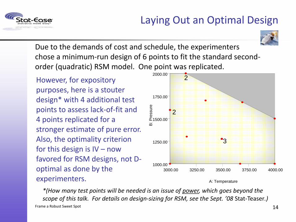
Due to the demands of cost and schedule, the experimenters chose a minimum-run design of 6 points to fit the standard second-order (quadratic) RSM model. One point was replicated.

Frame a Robust Sweet Spot 14

*(How many test points will be needed is an issue of power, which goes beyond the scope of this talk. For details on design-sizing for RSM, see the Sept. ’08 Stat-Teaser.)

However, for expository purposes, here is a stouter design* with 4 additional test points to assess lack-of-fit and 4 points replicated for a stronger estimate of pure error. Also, the optimality criterion for this design is IV – now favored for RSM designs, not D-optimal as done by the experimenters.

3000.00 3250.00 3500.00 3750.00 4000.00

1000.00

1250.00

1500.00

1750.00

2000.00

A: Temperature

B: P

ressure

3

2

2

Results

The following response surfaces were generated via re-simulation from predictive equations provided in coded form by the experimenters. The graphs closely resemble the published results for the key measures of dynamic pressure (Q) and total sensible enthalpy (Hts).

Frame a Robust Sweet Spot 15

1000.00

1250.00

1500.00

1750.00

2000.00

3000.00

3250.00

3500.00

3750.00

4000.00

1000

1200

1400

1600

1800

2000

2200

Q

A: Temperature B: Pressure

1000.00

1250.00

1500.00

1750.00

2000.00

3000.00

3250.00

3500.00

3750.00

4000.00

400

500

600

700

800

900

1000

H

ts

A: Temperature B: Pressure

Sweet Spot (Hypothetical)

The customer requirements have not been revealed, but assume they are represented by the graphical overlay shown below.

Frame a Robust Sweet Spot 16

3000.00 3250.00 3500.00 3750.00 4000.00

1000.00

1250.00

1500.00

1750.00

2000.00 Overlay Plot

A: Temperature

B: P

ressure

Q: 1400

Q: 1600

Hts: 650 Hts: 750 3

2

2

Robust Sweet Spot

To be more conservative (robust) in framing the sweet spot, superimpose the confidence intervals (CI) – a function of the underlying standard deviation (provided by the original publication) and the power of the experiment design (stronger in our re-simulation). The flag in the center might mark a good place to operate!

Frame a Robust Sweet Spot 17

3375.00 3450.00 3525.00 3600.00 3675.00

1100.00

1200.00

1300.00

1400.00

1500.00Overlay Plot

A: Temperature

B:

Pre

ss

ure

Q: 1400.000

Q: 1600.000

Q CI: 1400.000

Q CI: 1600.000

Hts: 650.000

Hts: 750.000

Hts CI: 650.000

Hts CI: 750.000

3

Q: 1495.473Hts: 698.972X1 3522.70X2 1300.97

Conclusion

Via application of response surface methods (RSM) experimenters in the field of test and evaluation can frame an operating window (aka “sweet spot” or “design space”). To be more conservative (robust), shade out the regions that fall within the confidence intervals of the boundary lines.

Frame a Robust Sweet Spot 18

Statistics Made Easy®

Best of luck for your experimenting!

Thanks for listening!

-- Mark

Frame a Robust Sweet Spot 19

Mark J. Anderson, PE, CQE Stat-Ease, Inc.

mark@statease.com