1

Graph-based Proprioceptive Localization Using a DiscreteHeading-Length Feature Sequence Matching Approach

Hsin-Min Cheng and Dezhen Song

Abstract—Proprioceptive localization refers to a new class ofrobot egocentric localization methods that do not rely on theperception and recognition of external landmarks. These methodsare naturally immune to bad weather, poor lighting conditions,or other extreme environmental conditions that may hinderexteroceptive sensors such as a camera or a laser ranger finder.These methods depend on proprioceptive sensors such as inertialmeasurement units (IMUs) and/or wheel encoders. Assisted bymagnetoreception, the sensors can provide a rudimentary estima-tion of vehicle trajectory which is used to query a prior knownmap to obtain location. Named as graph-based proprioceptivelocalization (GBPL), we provide a low cost fallback solution forlocalization under challenging environmental conditions. As arobot/vehicle travels, we extract a sequence of heading-lengthvalues for straight segments from the trajectory and matchthe sequence with a pre-processed heading-length graph (HLG)abstracted from the prior known map to localize the robot undera graph-matching approach. Using the information from HLG,our location alignment and verification module compensatesfor trajectory drift, wheel slip, or tire inflation level. We haveimplemented our algorithm and tested it in both simulated andphysical experiments. The algorithm runs successfully in findingrobot location continuously and achieves localization accurate atthe level that the prior map allows (less than 10m).

I. INTRODUCTION

Localization is a critical navigation function for vehicles orrobots in urban area. Common localization methods employglobal position system (GPS), a laser ranger finder, and a cam-era which are exteroceptive sensors relying on the perceptionand recognition of landmarks in the environment. However,high-rise buildings may block GPS signals. Poor weather andlighting conditions may challenge all exteroceptive sensors.What is needed is a fallback solution that enables vehiclesto localize themselves under challenging conditions. Thiscomplements existing exteroceptive sensor-based localizationmethods. Inspired by biological systems, we combine proprio-ceptive sensors, such as inertial measurement units (IMU) andwheel encoders, with magnetoreception, to develop a map-based localization method to address the problem, which isnamed as graph-based proprioceptive localization (GBPL).

In a nutshell, our new GBPL method employs the proprio-ceptive sensors to estimate vehicle trajectory and match it witha prior known map. However, this is non-trivial because 1)there is a significant drift issue in the dead reckoning processand 2) the true vehicle trajectory does not necessarily matchthe street GPS waypoints on the map due to the fact that astreet may contain multiple lanes and street GPS waypoints

H. Cheng and D. Song are with CSE Department, Texas A&M Univer-sity, College Station, TX 77843, USA, Emails: hmcheng@tamu.edu anddzsong@cs.tamu.edu.

This work was supported in part by National Science Foundation underNRI-1925037.

Query Sequence

(Heading/Length)

...

Heading-Length Graph

Road Map

(GPS waypoints)

Vehicle Trajectory

(IMU/Compass/

Wheel Encoder)

...

...

...

Input Graph Matching Output

...

Vehicle Location

Aligned location Trajectory

Estimated LocationIntersection GPS Waypoint

Fig. 1. An illustration of GBPL method. Left: our inputs include a priorknown map and the trajectory estimated from an IMU, a compass, and awheel encoder. Middle: we process the prior map in to a straight segmentconnectivity graph and also the trajecory into a query sequence of headingsand lengths of straight segments. Right: Aligned trajectory to the map aftergraph matching.

may be inaccurate. This determines that a simple trajectorymatching would not work. Instead, we focus on matching fea-tures which are straight segments of the trajectory (Fig. 1). Wekeep track of connectivity, heading and length of each segmentwhich converts the trajectory to a discrete and connected querysequence. This allows us to formulate the GBPL problemas a probabilistic graph matching problem. To facilitate theBayesian graph matching, we pre-process the prior knownmap consisting of GPS waypoints into a heading-length graph(HLG) to capture the connectivity of straight segments andtheir corresponding heading and length information. As therobot travels, we perform sequential Bayesian probabilityestimation until it converges to a unique solution. With globallocation obtained, we track robot locations continuously andalign the trajectory with HLG to bound error drift.

We have implemented our algorithm and tested it in physicalexperiments using our own collected data and an open dataset.The algorithm successfully and continuously localizes therobot. The experimental results show that our method out-performs in localization speed and robustness when comparedwith the counterpart in [1]. The algorithm achieves localizationaccurate at the level that the prior map allows (less than 10m).

The rest of the paper is organized as follows. After areview of related work in Section II, we define the problemin Section III. We introduce overall system design and detailGBPL in Section IV. We validate our system and algorithmwith simulation and physical experiments in Section V andconclude the paper in Section VI.

II. RELATED WORK

Our GBPL is related to localization using different sensormodalities, dead-reckoning, and map-based localization.

2

We can classify the localization methods into two categoriesbased on sensor modalities: exteroceptive sensors and pro-prioceptive sensors. Exteroceptive sensors mainly rely on theperception and recognition of landmarks in the environmentto estimate location. Mainstream exteroceptive sensors includecameras [2]–[4] and laser range finders [5]–[7]. These methodsare often challenged by poor lighting conditions or weatherconditions. GPS receiver [8], [9] is another commonly-usedsensor but it malfunctions when the vehicle travels close tohigh-rise buildings or inside tunnels. On the other hand, propri-oceptive sensors, such as IMUs [10] and wheel encoders [11],are inherently immune to external conditions. However, theyare more susceptible to error drift and suffer from limitedaccuracy. Recent sensor fusion approaches that combine anexteroceptive sensor, such as a camera or a laser ranger finder,with a proprioceptive sensor such as an IMU, greatly improvesystem robustness and become popular in applications [12].However, the sensor fusion approaches still strongly dependon exteroceptive sensor and cannot handle the aforementionedchallenging conditions.

To utilize proprioceptive sensors for navigation, deadreckoning integrates sensor measurements to computerobot/vehicle trajectory. The sensor measurements often in-clude readings from accelerometers, gyroscopes, and/or wheelencoders [13]. There are many applications using the deadreckoning approach such as autonomous underwater vehicles(AUVs) [14] and pedestrian step measurement [15], [16]. Toestimate the state of the robot/vehicle, filtering-based schemessuch as unscented Kalman filter (UKF) [17] and particle filter(PF) [18], [19] are frequently employed. However, the natureof dead reckoning causes it to inevitably accumulate errorsover time and lead to significant drift. To reduce the error drift,different methods have been proposed such as applying veloc-ity constraint on wheeled robots [20] and modeling the wheelslip for skid-steered mobile robots [13]. These approacheshave reduced error drift but cannot remove it completely. Errorstill accumulates over time and causes localization failure. Tofix the issue, we will show that drift can be bounded to mapaccuracy level by using map matching if the filtering-basedapproach with graph matching are combined.

Our method is a map-based localization [2], [21]–[24].According to [25], map representation can be classified intotwo categories: the location-based and the feature-based.The location-based maps are represented with specific lo-cations of objects. For example, those existing geographicmaps consisted of coordinate of locations such as Open-StreetMaps™ (OSM) [26] and Google Maps [27]. Geographicmaps have been widely used to improve upon GPS mea-surements and there are common measures being used suchas point-to-point, point-to-curve, curve-to-curve matching oradvanced techniques [28]. The feature-based map is consistedwith features of interest with its location. An example is ORBfeatures [29] for visual simultaneous localization and mapping.In this work, we extract heading-length graph from geographicmaps which converts a location-based map to a feature-basedmap to facilitate robust localization which also reduces graphsize to speed up computation in the process.

Closely-related works include [21], [30], [31], which focus

on map-aided localization using proprioceptive sensors formobile robots. In [30], only vehicle speed and speed limitinformation from map are used as a minimal sensor setup.However, known initial position is required and the methodachieves an accuracy of around 100 meters. In [21], thevelocity from wheel encoder and steering angles are used forodometry and a particle filter based map matching schemehelps estimate vehicle positions. It does not consider velocityerrors from the wheel encoder such as slippery or inflationlevels. In [31], odometer and gyroscope readings are usedfor extended Kalman filter (EKF)-based dead reckoning anda map is used to correct errors when driving a long distanceor turning at road intersections. The average positional erroris 5.2 meters, but it again requires an initial position fromGPS. It is worth noting that our localization solution does notrequire a known initial position.

This paper is a significant improvement over our earlywork [1] where only heading sequence is used and localiza-tion is only intermittent for turns. The new method enablescontinuous localization by considering wheel encoder inputsand is less limited by map degeneracy (e.g. rectilinear envi-ronments). Also, we bound error drift in location alignmentand verification after graph matching.

III. PROBLEM FORMULATION

A. Scenarios and Assumptions

In our set up, a robot or a vehicle (We interchangeably use“robot” and “vehicle.”) is navigating in a poor weather condi-tions such as a severe thunderstorm or a whiteout snowstorm.No other exteroceptive sensors work properly. However, it isstill necessary for the vehicle to find its location.

The vehicle/robot is equipped with an IMU, a digital com-pass or a magnetometer, and an on-board diagnostics (OBD)scanner which provides velocity feedback while navigating inan area with a given prior road map, e.g. OpenStreetMaps(OSM) [26]. We have the following assumptions:

a.0 The vehicle is able to navigate in the environment andmake turns at appropriate locations. If needed, the vehi-cle is willing to change its course by making additionalturns to assist our algorithm to find its location.

a.1 The prior road map contains straight segments in mostpart of its streets and streets are not strict grids withequal side lengths.

a.2 The robot is a nonholonomic system,. i.e. it only per-forms longitudinal motion without lateral or verticalmotions.

a.3 The IMU and the compass are co-located, pre-calibrated,and fixed at the vehicle geometric center.

a.4 The IMU, compass, and velocity readings are synchro-nized and time-stamped.

As part of the input of the problem, a prior road mapconsisting of a set of roads with GPS waypoints is required.The typical distance between adjacent waypoints is around20m.

B. Nomenclature

Common notations are defined as follows,

3

*

B2) Heading-Length Sequence

GenerationHeading Change?

B. Query Sequence Generation (QSG) Thread

I =1? G

StartSet I = 0 G

[ p ,v ,Θ ] II I TIMU ω

Compass Φ

a,

Vehicle Velocity

C1) Graph Matching

C. Global Localization (GL) Thread

Unique solution ?

YesStart

=ø Set

No

x G

Yes No

YesGo D1)

Go C1)

Set I = 1Terminate

G

No

GL started? Yes

NoStart GL

LAV started? Yes

NoStart LAV

Start LAV

v

EKF Predict/Update

State/Covariance Initialization

B1) EKF

x G

Construct Heading-Length Graph

Prior MapMhMp

A. Construct Heading-Length Graph

HLG

Θ q DqQ ={ , }

QQ

C2) Candidate Vertex

Selection

D1) Virtual Start-End Point

Estimation

D. Location Alignment and Verification (LAV) Thread

YesStart

Good Matching?

No Set I = 0Terminate

*

GT*

D3) Scale and Slip Factor Estimation

se

Mp

D2) Location Alignment and

Verification

Fig. 2. System Diagram

• Mp := {xm = [xm,ym]T ∈R2|m∈M } represents the prior

road map which is a set of GPS positions where M isthe position index set. Note that these GPS positions aremap points instead of live GPS inputs. We do NOT useGPS receiver in our algorithm design.

• a = {a j ∈ R3| j = 0,1, · · · ,N j} and ω = {ω j ∈ R3| j =0,1, · · · ,N j} denote accelerometer readings and gyro-scope angular velocities from the IMU, respectively.

• φ = {φ jφ ∈R| jφ = 0, · · · ,bN jcφc} denotes compass readings

where cφ ≥ 1 since a compass often has lower samplingfrequency than that of the IMU.

• v = {v jv ∈R| jv = 0, · · · ,bN jcvc} denotes wheel speed read-

ings from OBD where cv ≥ 1 because it has a lowersampling frequency than that of IMU. And v jv is the speedat midpoint of car rear wheels.

• Mh = {Vh,Eh} denotes the HLG where Vh is the vertexset and Eh and is the edge set.

• Q = {Θq,Dq} denotes the query heading-length sequencewhich consists of the segmented heading-length sequence.Θq is the set of heading sequence and Dq is the set oftravel length sequence.

• Ck represents the candidate vertex set where k = 1, · · · ,nis the length of the query sequence.

The GBPL problem is defined as follows.

Problem 1. GivenMp, a, ω , φ and v, localize the robot afterits heading changes. As its localized, report robot locationcontinuously.

IV. GBPL MODELING AND DESIGN

Our system diagram is illustrated in Fig. 2 which con-sists of four main building blocks: HLG construction, querysequence generation (QSG) thread, global localization (GL)thread, and location alignment and verification (LAV) thread.HLG construction is shaded in light gray which converts theprior geographic map into an HLG which runs only once inadvance. For the rest shaded in dark gray, we refer to them asthreads because they can be implemented as a parallel multi-threaded application. The QSG thread runs EKF constantlyat the back end as the system receives sensory readings a,ω , φ and v and outputs the estimated trajectory. GL thread

searches for the global location on a turn-by-turn basis. GLthread performs Bayesian graph matching between the querysequence extracted from the trajectory and the HLG. Afterthe global location is obtained, GL terminates and LAV alignsthe latest segment with the map and uses the result to rectifyerror drifting in the EKF in QSG. If no satisfying alignmentis found, LAV terminates and the system restarts GL. In fact,GL thread and LAV thread work alternatively depending onwhether the robot is localized or not. We begin with HLGconstruction.

A. HLG Construction

We pre-process map Mp to construct an HLG to facilitateheading-length matching. There are three reasons for usingHLG instead of matching on Mp directly.• First, the vehicle trajectory may not exactly match withMp. Since Mp and most maps do not have lane-levelinformation, the discrepancy between the estimated tra-jectory andMp is non-negligible which makes the directtrajectory-to-map matching unreliable. Fig. 3 shows anexample. For the same route, the trajectories may bedifferent due to driving on different lanes, driver habit,traffic, etc.

• Second, matching trajectory with Mp directly is compu-tationally expensive because the searching space growswith the total number of GPS waypoint positions inMp.

• Third, the inevitably accumulated trajectory drift dete-riorates the matching quality and makes the matchingunreliable.

Therefore, we extract features from the map which are thelong straight segments and represent them as the HLG. Thisleads to a graph matching approach that can mitigate theinfluence of the aforementioned three issues. We start withHLG construction based on our prior work [1] where we haveestimated road curvature changes to capture orientation changeand construct a heading graph (HG). Build on [1], we augmentlength information in HG to construct HLG for heading-lengthmatching. Fig. 4 illustrates an example. For completeness,we provide an overview here and more detail descriptionof constructing the graph can be found in [1]. The HLGMh = {Vh,Eh} is a directed graph. A vertex vi ∈Vh represents

4

GPS Waypoint

Trajectory 1

Trajectory 2

Fig. 3. Map and trajectory discrepancy illustration. Given the trajectorygenerated by proprioceptive sensors, directly matching trajectory with the mapmay not be desirable. For the same route, trajectories 1 and 2 appear quitedifferently. Neither of them matches blue waypoints in the map.

di

θi

Xi

vi

xi,s

xi,e

Fig. 4. HLG illustration in color. The left figure shows a satellite imagewith road map consisted of GPS waypoints (blue dots) overlaying on top ofthe image and intersections represented in small black circles. We estimateroad curvature changes to capture heading change and construct HLG. As anexample, we color a long and straight segment with light blue and a curvesegment with light orange. The right figure shows the corresponding HLG,and we only employ long road segment vertices for localization.

a straight and continuous road segment with neither orientationchanges nor intersections. An edge ei,i′ ∈ Eh captures theconnectivity between nodes and characterizes the orientationchange between the two connected vertices vi and vi′ .Mh hastwo types of edges: road intersections and curve segments; andtwo types of vertices: long straight segment vertices and shorttransitional segment vertices. The short transitional segmentvertices are often formed between curve segments or curvedroads entering intersections.

To build Mh, we split each road at road intersectionsand further segment them into two types of segments tocapture orientation changes: straight segments and curved seg-ments [1]. With all roads segmented, we compute orientationand length for vertices corresponding to those long straightroad segments. Each vertex contains the following information

vi = {Xi,θi,di,bi}, (1)

where Xi = [xTi,s, · · · ,xTi,e]T contained all 2D waypoint positionsin GPS coordinates of the road segment with starting positionxi,s and ending position xi,e, orientation θi ∈ (−π,π] is theangle between the geographic north and the orientation ofthe road segment computed using Xi with a least squaresestimation method adopted from [1], di is road segment lengthwhich is computed. by

di = ||xi,s−xi,e||, (2)

and bi is the binary variable indicate if the vertex is a longroad segment. We only perform orientation estimation if di > tl

where tl is the threshold for road segment length. That is,

bi =

{1, di > tl ,0, otherwise.

(3)

Only long road segments (bi = 1) will be used in localizationwhich defines vertex subset Vh,l ⊆ Vh corresponding to longstraight segments. Note that θi depends on the robot travelingdirection and hence Mh is a directed graph.

The errors of GPS waypoints in each entry of Xi affect theaccuracy of θi and di. To track map uncertainties caused byGPS errors, we derive the distribution of θi and di using errorvariance propagation analysis [32]. We model GPS errors byusing Gaussian distribution and assuming GPS measurementnoises to be independent and identically distributed. We denotethe GPS measurement variance by σ2

g . According to [2],typical consumer grade navigation systems offer positionalaccuracy around σg = 10m. The distribution of θi that charac-terizes its uncertainty is

θi ∼N (µθi ,σ2θi), (4)

where σ2θi

is derived in [1]. And the distribution of di is

di ∼N (µdi ,σ2di) =N (µdi ,2σ

2g ). (5)

B. Query Sequence Generation (QSG) Thread

To localize the vehicle on Mh, we estimate the trajectoryfrom sensory readings with an EKF-based approach. Wethen generate a discrete query consisting of a heading-lengthsequence extracted from the EKF trajectory results. It is worthnoting that our method is not sensitive to the global driftof the EKF estimated trajectory because we only use shortsegmented trajectory to extract heading and length of itsstraight segments.

1) EKF-based Trajectory Estimation: Note that readingsfrom the IMU, the digital compass, and the vehicle velocity:a, ω , φ , and v, are the inputs to the EKF-based approach to es-timate vehicle trajectory [33]–[35]. To start the EKF, we needa stabilized initial compass reading φ0 to determine the initialvehicle orientation which can be obtained by driving on a longand straight segment of road (Assumption a.2). We define tworight-handed coordinate systems: IMU/compass device bodyframe {B} (also overlapping with vehicle geometric center),the fixed inertial frame {I} which shares its origin with {B}at the initial pose. Frame {I}’s X-Y plane is a horizontal planeparallel to the ground plane with Y axis pointing to magneticnorth direction and Z axis is vertical and points upward. Inthe state representation, let state vector Xs, j at time j be:

Xs, j := [pIj,v

Ij,Θ

Ij,s j]

T, (6)

which includes position pI = [x,y,z]T ∈ R3, velocity vI =[x, y, z]T ∈ R3, and the Euler angles Θ

I := [α,β ,γ]T in {I}in X-Y -Z order, and scale/slip factor (SSF) s. We define shere to address vehicle velocity error which can be caused bytire radius error such as inflation level, road slippery, etc. Thesuperscripts indicate in which frame the vector is defined. Thetransformation from {I} to {B} is the Z-Y -X ordered Euler

5

angle rotation. The state transition equations are described asfollows:

pIj = pI

j−1 + τω vI

vIj = vI

j−1 + τω(IBR(a)−G)

Θ j = Θ j−1 + τωIBE(ω)+ cγ

s j = s j−1,

(7)

where τω is the IMU sampling interval, G = [0 0 −9.8]T isthe gravitational vector, cγ = [0 0 φ0]

T is the initial orientationdetermined by φ0, I

BR is the rotation matrix from {B} to {I},and I

BE is the rotation rate matrix from {B} to {I}.For EKF observation models, we use velocity constraint

from vehicle movement, sensory readings φ and v, and es-timated scale by matching trajectory with map which will bediscussed in Section IV-D3. First, according to Assumptionsa.2 there is no lateral or vertical movements in {B}, thevelocities along Y axis and Z axis in {B} are set to be zeros.The velocity constraint is written as:

(BIR)2:3vI

j =[0 0

]T, (8)

where BIR2:3 is the second and third rows of B

IR.From the coordinate definition, the heading direction is

γ defined in {I} (last component of ΘI), we take compass

reading φ as its observation. In our physical system, compassreadings have a lower sampling frequency than that of the IMUreadings, we use the latest available reading. Also, compassreadings may be polluted by other magnetic fields, we canrecognize faulty readings by cross-validating compass readingswith IMU readings. We discard the faulty compass readingsif the difference between the estimated heading state andthe compass reading exceeds an threshold. With the cross-validated compass reading, we update heading direction γ by

γ j =

{φ jφ , if j = cφ jφφ jφ−1, otherwise.

(9)

We compensate SSF s j by estimating its value from alignedmap data after taking a turn. We will detail how to computesss f and its variance in Section IV-D3. For s, we have

s j = sss f , (10)

where sss f is the ratio of the trajectory length from the mapversus that from the query. Lastly, we take wheel velocity vas observations. Similar to φ that the sampling frequency islower than IMU readings, we have

||vIj||=

{s jv jv , if j = cv jvs jv jv−1, otherwise.

(11)

Combining (9), (8), (11), and (10), we complete the observa-tion model functions. The rest is to follow the standard EKFsetup. Fig. 5(a) shows the estimated EKF trajectory comparedwith the corresponding GPS ground truth trajectory. Note thatthe vehicle takes some additional turns to assist localization(Assumption a.0) and the trajectory is not the shortest.

-0.4 -0.2 0 0.2

km

-0.7

-0.6

-0.5

-0.4

-0.3

-0.2

-0.1

0

km

(a)

0 1 2 3 4 5 6

Time(sec) 104

100

150

200

250

300

350

0

0.2

0.4

0.6

0.8

1

(b)

-0.4 -0.2 0 0.2

km

-0.7

-0.6

-0.5

-0.4

-0.3

-0.2

-0.1

0

km

(c)

Fig. 5. (a) Trajectory estimation result: the red line is the GPS ground truth,and black line illustrates the EKF estimated trajectory. (b) Query headingrepresentations. Blue line is estimated heading, black vertical lines are indiceswhere data segmented, red lines mark out stable heading segments andunmarked segments are detected turns. (c) Corresponding travel heading andlength segment representations. Different segments are marked in differentcolors.

2) Heading-Length Sequence Generation: With the esti-mated trajectory, we generate query heading-length sequenceby capturing vehicle heading changes. We adopt the methodfor heading sequence generation from [1] and augment cor-responding length sequence in this work. To improve therobustness, we only keep headings when the vehicle is trav-eling on long and straight road segments. This means theheadings should be stable and constant in a long stretch oftravel time and corresponding travel distance is long. Fromthe coordinate definition, the headings is γ in {I} and isdenoted by γ0: j. To obtain the query sequence, we segmentγ0: j to get stable headings and remove false positive headingsthat do not correspond to long and straight road segments. InFig. 5(b), red horizontal segments are detected stable headings.Hence we obtain the set of query heading sequence which isdenoted by Θq = {Θq,k|k = 1, · · · ,n} where k is query dataindex, n is the number of straight segments. Each subsetΘq,k corresponding to continuous observations from EKFrepresents a straight segment. At the same time, we generatethe corresponding travel length sequence which is denoted byDq = {dq,k|k = 1, · · · ,n} where dq,k is the travel length of thesegmented route (e.g. colored segments in Fig. 5(c)).

The query heading-length sequence Q = {Θq,Dq} is con-sists of the segmented heading-length sequence. The uncer-tainty of query sequence Q is obtained from EKF varianceestimation. For Θq, we define θq,k as the sample mean ori-entation of segment Θq,k which contains nθq,k observations of

6

random variable θq,k. θq,k has it covariance matrix obtainedfrom EKF. For Dq, the variance of dq,k can also be derivedfrom EKF and we denote it by σ2

dq,k. Those variables will be

used later in the analysis part.It is worth noting that each entry of the sequence is not

sensitive to the overall trajectory drift due to local trajectorysegment computation. When segmenting into short segments,the drift in each segment is smaller compare to the overalltrajectory drift. The resulting sequence also can be understoodas local features for the trajectory. Also, reducing the queryto the discrete feature sequence helps in reducing computationcomplexity.

C. Global Localization Thread

1) GL Overview: With the query sequence obtained fromon-board sensors, we are ready to match it with sequenceson the HLG to search for the actual location. This is a graphmatching problem. In the GL thread, we localize the robotwhen the robot changes its heading which is the moment thequery sequence grows its length. It is worth noting that GL isan intermittent localization. The continuous localization willbe address later in the paper.

Given the query heading-length sequence, we search forthe best match of heading-length sequence in the HLG Mh.For any long straight candidate vertex in Vh,l , we match thequery heading-length sequence with sequences of the verticesstarting at the candidate vertex. We discard candidate verticeswith poor matching. In each candidate sequence to querysequence matching, We model sensory and map uncertaintiesand formulate the matching process as a sequential hypothesistest problem. The result of GL depends on if a satisfyingmatching sequence can be found.

2) Graph Matching: The center part of GL is the matchingof query sequence and candidate sequence on the graph. Toachieve this, we expand the heading sequence matching in[1] to find the best heading-length matching in Mh. Givenquery sequence Q = {Θq,Dq}= {(θq,k,dq,k)|k = 1, · · · ,n}, letus denote a candidate heading-length vertex sequence in Mhby M := {Θ,D}= {(θk,dk)|k = 1, · · · ,n} correspondingly. Asa convention in this paper, for random vector ?, µ? representsits mean vector. Following the convention, mean matrix of Qis defined as µQ = [µT

Θq,µT

Dq]T where µΘq = [µθq,1 , · · · ,µθq,n ]

T

and µDq = [µdq,1 , · · · ,µdq,n ]T. The mean matrix of M is de-

noted by µM = [µTΘ,µT

D ]T where µΘ = [µθ1 , · · · ,µθn ]

T andµD = [µd1 , · · · ,µdn ]

T.Due to independent measurement noises, the conditional

matching probability between query sequence Q := {Θq,Dq}and a candidate sequence M := {Θ,D} on HLG Mh is

P(µQ = µM|Q,M)

= P(µΘq = µΘ|Θq,Θ)P(µDq = µD|Dq,D). (12)

From [1], the conditional heading matching probability be-tween Θq and Θh is

P(µΘq = µΘ|Θq,Θ) ∝

n

∏k=1

fT (t(θq,k,θk)), (13)

due to independent sensor noises and fT (t(θq,k,θk)) is theprobability density function (PDF) of Student’s t-distribution.For length matching, the conditional matching probabilitybetween Dq and D is

P(µDq = µD|Dq,D) ∝

n

∏k=1

f (z(dq,k,dk)), (14)

where f (·) is the PDF of standard normal distribution, andz(dq,k,dk) =

dq,k−dk√σ2

dk+σ2

dq,k

. Combining (13) and (14) and recall-

ing that n is the number of straight segments in the querysequence, we rewrite (12) as follows,

P(µQ = µM|Q,M) ∝

n

∏k=1

fT (t(θq,k,θk)) f (z(dq,k−dk)). (15)

3) Candidate Vertex Selection: To select on candidate ver-tices during matching, we perform statistical hypothesis testingto remove unlikely matchings. According to (12), sequencematching is considered as multiple pair matching. For eachpair ({θk,dk},{θq,k,dq,k}), it is a hypothesis testing

H0 : [µθq,k ,µdq,k ]T = [µθk ,µdk ]

T

H1 : otherwise. (16)

Hypothesis H0 can be seen as two null hypotheses: H0,θ :µθq,k = µθk and H0,d : µdq,k = µdk . We perform two individualtests separately with significance level 1−α where α is a smallprobability. Both H0,θ and H0,d are two-tailed distributions. Wechoose tα/2,ν as the t-statistic with a cumulative probability of(1− α

2 ) where ν is the degrees of freedom (DoF) and zα/2as the z-statistic with a cumulative probability of (1− α

2 ). Wereject H0 if

(|t(θk,θq,k)|> tα/2,ν)∨ (|z(dk,dq,k)|> zα/2). (17)

By sequentially applying the hypothesis testing on each cor-responding pair ({θk,dk},{θq,k,dq,k}) from query sequence Qand candidate sequence M on HLGMh, we determine whetherM represents the actual trajectory. Fig. 6 has shown that usingthe joint distribution of heading and length significantly reducethe number of solutions in the matching process.

(a) (b)

Fig. 6. An example of global localization. (a) The candidate locations usingheading matching (green dots), length matching (black circle). We showthat performing heading-length matching (locations with green dot and blackcircle) helps reducing candidates. (b) The candidate localization is reducedto the single solution if the joint distribution between heading and length isused.

7

In the matching process, we might get many candidatesolutions because the hypothesis test is conservative in rejec-tion. To address the problem and check if we converge to aunique solution, we classify the computed probabilities of (12)into two groups using the Ostu method [36]. The number ofsolutions is the group size. If the group with higher probabilityhas only one candidate then the vehicle is localized. Otherwise,it means that the group with higher probability contains severaltrajectories with higher probabilities. It indicates that moreobservations are needed to localize the vehicle.

4) GL Algorithm: We summarize the heading-lengthmatching method in Algorithm 1. In a nutshell, as we sequen-tially match the vertex down the query sequence, we compareit with the out-neighbor of remaining vertices on the graphusing breadth-first search.

Note that vertex vi may have adjacent vertices with sameorientation. For example, consider the vehicle reaches a longstraight road (with road intersections). This long straight roadcorresponds a set of vertices with same orientation. We denotethe set of straight path start from vi by Vs.

To reuse the computed information as the query sequencegrows, we define the candidate vertex information set Ck wherek = 1, · · · ,n is the length of the query sequence. The candidatevertex set is denoted by Ck = {{vi,VM,i, pi}|i = 1, · · · ,nCk},where each element in Ck record the candidate vertex vi (thestarting vertex of the trajectory/path), VM,i is the set of vertexpath, and the matching probability pi in (12) and nCk is thecardinality of Ck. To initialize, we set C0 := {{vi, /0, 1

|Vh,l |}|i =

1, · · · , |Vh,l |} because each vertex in Vh,l is equally likely tobe the path starting vertex. The computational complexity ofcalculating each term in (12) is O(1) using the alias samplingmethod [37]. The upper bound of candidate vertex cardinalityis |Vh,l | and thus it takes O(|Vh,l |) to compute probabilityof all candidate vertices. The size of straight path set takesO(|Vs|) which is related to variation of map road headings inSec. IV-C6. With little variation in headings (e.g. Manhattanstreets), |Vs| is larger. On the contrary, |Vs| is small comparedto |Vh,l | with large variation in road headings. In this case,O(|Vs|) = O(1). The classification of probabilities into twogroups is O(|Vh,l |) using Hoare’s selection algorithm.

We summarize the computational complexity of Algo-rithm 1 in Lemma 1.

Lemma 1. The computation complexity of the heading-lengthmatching is O(n|Vs||Vh,l |).

5) Localization Analysis: The remaining problem iswhether this sequence of hypothesis testing would convergeto the true trajectory as the length of the sequence grows.To analyze this, let us define three binary events: Ak = 1 ifµdq,k = µdk , Bk = 1 if µθq,k = µθk , and Ck = 1 if vertex k in Mhis the actual location. The joint event C1 · · ·Cn = 1 is to sayM := {Θ,D} represent the true trajectory, whereas we knowA1 · · ·AnB1 · · ·Bn from sequence matching. In the analysis, wedenote nv = |Vh,l | as the cardinality of Vh,l and nb as theexpected number of neighbors for each vertex. We describemap/trajectory property in a rudimentary way by assumingkd levels of distinguishable discrete headings in [0,2π) andkl levels of distinguishable discrete road lengths. Each vertex

Algorithm 1: Heading-length Graph MatchingInput: Mh = {Vh,Eh} and Q = {Θq,Dq}Output: Ck or vehicle location, IG

1 C0 := {{vi, /0, 1|Vh,l |}|i = 1, · · · , |Vh,l |} O(1)

2 Initialize IG = 0 O(1)3 for k = 1, · · · ,n do O(n)4 Ck ← /0; O(1)5 for i = 1, · · · ,nCk−1 do O(|Vh,l |)6 if k == 1 then7 Access straight path set Vs start from vi; O(1)8 else9 vi′ ← last vertex in path VM,i O(1)

10 Vi′ ← adjacent verteices of vi′ ( with different angles); O(1)11 Access straight path set Vs start from each vertex in Vi′ ; O(1)

12 for Vs ∈ Vs do O(|Vs|)13 Access θs and ds of Vs; O(1)14 compute p← fT (t(θs,θq,k)) f (z(ds,dq,k)) O(1)15 if Pass hypothesis testing in (16) then16 Update matching probability pi′ ← pi · p O(1)17 VM,i′ ← Append Vs to VM,i O(1)18 Ck ← Ck ∪{vi,VM,i′ , pi′} O(1)

19 Classify probabilies in (12) of Ck using Otsu’s method; O(|Vs||Vh,l |)20 Remove group in Ck with lower probabilities; O(1)21 if |Ck |> 1 then22 Return Ck ; O(1)23 else24 Set IG = 1; O(1)25 Return vehicle location; O(1)

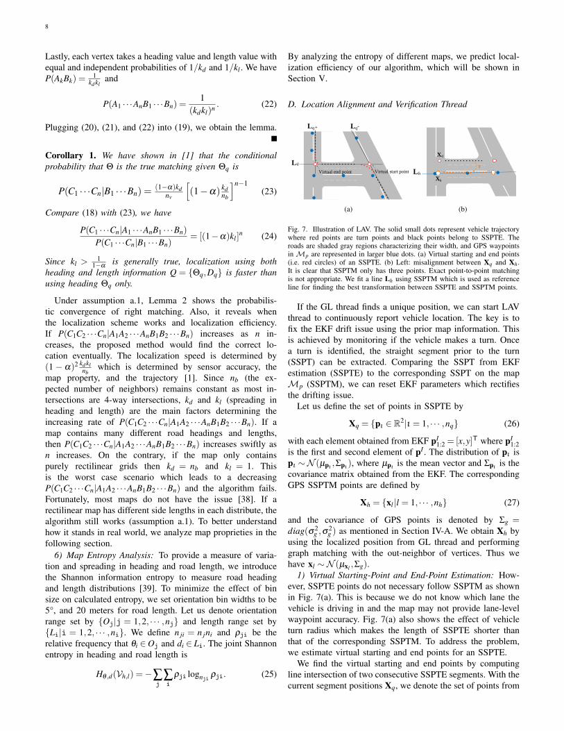
takes a heading value and length value with equal probabilitiesof 1/kd and 1/kl correspondingly. Generally speaking, weknow nv� kd ≥ nb and nv� kl ≥ nb for most maps. we havethe following lemma.

Lemma 2. The conditional probability that M = {Θ,D} is thetrue matching sequence given that Q = {Θq,Dq} matches Mis,

P(C1 · · ·Cn|A1 · · ·AnB1 · · ·Bn) =(1−α)2kdkl

nv

[(1−α)2 kdkl

nb

]n−1

(18)

Proof: Applying the Bayesian equation, we have

P(C1 · · ·Cn|A1 · · ·AnB1 · · ·Bn) =

P(A1 · · ·AnB1 · · ·Bn|C1 · · ·Cn)P(C1 · · ·Cn)

P(A1 · · ·AnB1 · · ·Bn). (19)

Indeed P(A1 · · ·AnB1 · · ·Bn|C1 · · ·Cn) is the conditional proba-bility that a correct matched sequence survives n hypothesistests in (16). Due to independent measurement noises, we haveP(A1B1|C1) = (1−α)2. Besides, these tests are independentdue to independent sensor noises, we have

P(A1 · · ·AnB1 · · ·Bn|C1 · · ·Cn) = (1−α)2n. (20)

Joint probability P(C1 · · ·Cn) is actually the unconditionalprobability of being correct locations. We know P(C1) = 1/nvgiven there are nv possible solutions, and P(C2|C1) = 1/nbbecause there are nb neighbors of C1. By induction,

P(C1 · · ·Cn) =1

nn−1b

1nv. (21)

8

Lastly, each vertex takes a heading value and length value withequal and independent probabilities of 1/kd and 1/kl . We haveP(AkBk) =

1kdkl

and

P(A1 · · ·AnB1 · · ·Bn) =1

(kdkl)n . (22)

Plugging (20), (21), and (22) into (19), we obtain the lemma.

Corollary 1. We have shown in [1] that the conditionalprobability that Θ is the true matching given Θq is

P(C1 · · ·Cn|B1 · · ·Bn) =(1−α)kd

nv

[(1−α) kd

nb

]n−1(23)

Compare (18) with (23), we have

P(C1 · · ·Cn|A1 · · ·AnB1 · · ·Bn)

P(C1 · · ·Cn|B1 · · ·Bn)= [(1−α)kl ]

n (24)

Since kl >1

1−αis generally true, localization using both

heading and length information Q = {Θq,Dq} is faster thanusing heading Θq only.

Under assumption a.1, Lemma 2 shows the probabilis-tic convergence of right matching. Also, it reveals whenthe localization scheme works and localization efficiency.If P(C1C2 · · ·Cn|A1A2 · · ·AnB1B2 · · ·Bn) increases as n in-creases, the proposed method would find the correct lo-cation eventually. The localization speed is determined by(1− α)2 kdkl

nbwhich is determined by sensor accuracy, the

map property, and the trajectory [1]. Since nb (the ex-pected number of neighbors) remains constant as most in-tersections are 4-way intersections, kd and kl (spreading inheading and length) are the main factors determining theincreasing rate of P(C1C2 · · ·Cn|A1A2 · · ·AnB1B2 · · ·Bn). If amap contains many different road headings and lengths,then P(C1C2 · · ·Cn|A1A2 · · ·AnB1B2 · · ·Bn) increases swiftly asn increases. On the contrary, if the map only containspurely rectilinear grids then kd = nb and kl = 1. Thisis the worst case scenario which leads to a decreasingP(C1C2 · · ·Cn|A1A2 · · ·AnB1B2 · · ·Bn) and the algorithm fails.Fortunately, most maps do not have the issue [38]. If arectilinear map has different side lengths in each distribute, thealgorithm still works (assumption a.1). To better understandhow it stands in real world, we analyze map proprieties in thefollowing section.

6) Map Entropy Analysis: To provide a measure of varia-tion and spreading in heading and road length, we introducethe Shannon information entropy to measure road headingand length distributions [39]. To minimize the effect of binsize on calculated entropy, we set orientation bin widths to be5°, and 20 meters for road length. Let us denote orientationrange set by {Oj|j = 1,2, · · · ,nj} and length range set by{Li|i = 1,2, · · · ,ni}. We define n ji = n jni and ρji be therelative frequency that θi ∈Oj and di ∈ Li. The joint Shannonentropy in heading and road length is

Hθ ,d(Vh,l) =−∑j

∑i

ρji lognji ρji. (25)

By analyzing the entropy of different maps, we predict local-ization efficiency of our algorithm, which will be shown inSection V.

D. Location Alignment and Verification Thread

Lq

Lq-Lq+

LhVirtual start pointVirtual end point

Xq

Xh

L h

X h

T

(a)

Lq

Lq-Lq+

LhVirtual start pointVirtual end point

Xq

Xh

L h

X h

T

(b)

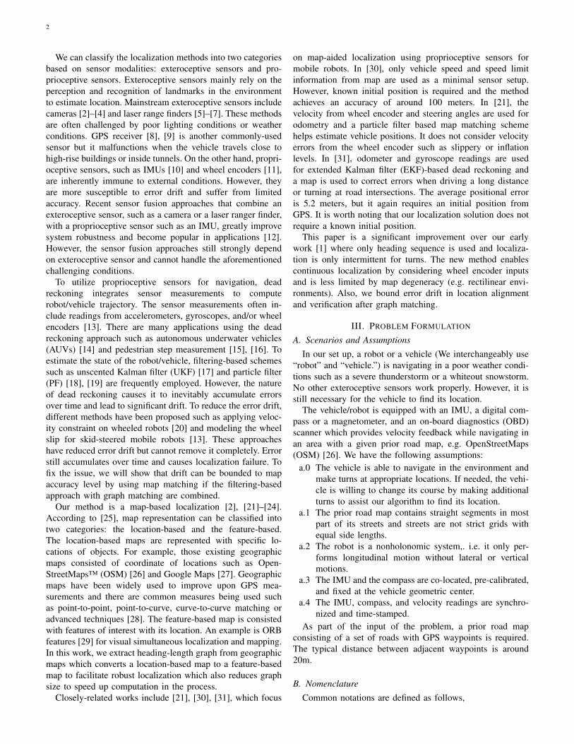
Fig. 7. Illustration of LAV. The solid small dots represent vehicle trajectorywhere red points are turn points and black points belong to SSPTE. Theroads are shaded gray regions characterizing their width, and GPS waypointsin Mp are represented in larger blue dots. (a) Virtual starting and end points(i.e. red circles) of an SSPTE. (b) Left: misalignment between Xq and Xh.It is clear that SSPTM only has three points. Exact point-to-point matchingis not appropriate. We fit a line Lh using SSPTM which is used as referenceline for finding the best transformation between SSPTE and SSPTM points.

If the GL thread finds a unique position, we can start LAVthread to continuously report vehicle location. The key is tofix the EKF drift issue using the prior map information. Thisis achieved by monitoring if the vehicle makes a turn. Oncea turn is identified, the straight segment prior to the turn(SSPT) can be extracted. Comparing the SSPT from EKFestimation (SSPTE) to the corresponding SSPT on the mapMp (SSPTM), we can reset EKF parameters which rectifiesthe drifting issue.

Let us define the set of points in SSPTE by

Xq = {pι ∈ R2|ι = 1, · · · ,nq} (26)

with each element obtained from EKF pI1:2 = [x,y]T where pI

1:2is the first and second element of pI . The distribution of pι ispι ∼N (µpι

,Σpι), where µpι

is the mean vector and Σpιis the

covariance matrix obtained from the EKF. The correspondingGPS SSPTM points are defined by

Xh = {xl |l = 1, · · · ,nh} (27)

and the covariance of GPS points is denoted by Σg =diag(σ2

g ,σ2g ) as mentioned in Section IV-A. We obtain Xh by

using the localized position from GL thread and performinggraph matching with the out-neighbor of vertices. Thus wehave xl ∼N (µxl ,Σg).

1) Virtual Starting-Point and End-Point Estimation: How-ever, SSPTE points do not necessary follow SSPTM as shownin Fig. 7(a). This is because we do not know which lane thevehicle is driving in and the map may not provide lane-levelwaypoint accuracy. Fig. 7(a) also shows the effect of vehicleturn radius which makes the length of SSPTE shorter thanthat of the corresponding SSPTM. To address the problem,we estimate virtual starting and end points for an SSPTE.

We find the virtual starting and end points by computingline intersection of two consecutive SSPTE segments. With thecurrent segment positions Xq, we denote the set of points from

9

previous and next SSPTE segments by Xq− and Xq+ , respec-tively. Applying line fitting to Xq, Xq− , and Xq+ , we obtainthree 2D lines Lq, Lq− , and Lq+ , respectively. We parameterizeeach line by two reference points. Thus we denote Lq =[aTq ,bT

q ]T, Lq− = [aTq− ,b

Tq− ]

T, and Lq+ = [aTq+ ,bTq+]

T. Also, theline direction vectors are vq = bq−aq, vq+ = bq+ −aq+ , andvq− = bq−−aq− . Finding the intersection between Lq and Lq−

allows us to obtain the virtual starting point. We denote thevirtual starting point of Xq by ps.

ps = aq−v⊥q− .(aq−a−q )

v⊥q− .vqvq, (28)

where · is dot product and v⊥q− is the perp operator of vq− .Similarly, the intersection between Lq and Lq+ gives us thevirtual end point pe. We have

pe = aq−v⊥q+ .(aq−a+q )

v⊥q+ .vqvq, (29)

where v⊥q+ is the perp operator of vq+ . When SSPTE isconnected with an curve segment (e.g. caused by vehicle turn),we add ps and pe to Xq to help alignment process. ps and pebecome the first and the last points in Xq, respectively.

2) Location Alignment and Verification: With augmentedXq, we can match Xq to Xh to rectify drifting issue by findingthe transformation T between them (see Fig. 8). Here T is 3-DoF rigid body transformation represented by a 2x2 rotationmatrix R, and a 2x1 translation vector t,

T(x) := Rx+ t, (30)

where x is a 2D point. Xq usually contains significantlymore entries than that of Xh due to its higher samplingfrequency (nq� nh). Directly matching two point sets is notthe best solution. Instead, we fit a line through points in Xhand minimizing the distance of all points in Xq to this line(Fig. 7(b)).

Let us denote Lh = [aTh ,bTh ]

T where ah and bh are tworeference points on the line. For every point p j in Xq, thepoint after transformation is denoted by T(pι). The point-to-line distance between T(pι) and Lh is defined as

d⊥(T(pι),Lh) =||(ah−T(pι)× (ah−bh)||

||ah−bh||, (31)

where ‘×’ is the cross product and || · || is the L2 norm. Wedefine the cost function CT by

CT =

d⊥(T(ps),Lh)d⊥(T(p1),Lh)

...d⊥(T(pnq),Lh)d⊥(T(pe),Lh)

, (32)

and formulate the following optimization problem

arg minT

CTTΣ−1C CT +λ ||T(ps)−x1||+λ ||T(pe)−xnh ||, (33)

where ΣC = diag(σ2d⊥,ps

, · · · ,σ2d⊥,pe

), β is a nonnegativeweight, and x1 and xnh are the first and the last entries in

0 0.2 0.4 0.6km

-0.2

-0.1

0

0.1

0.2

0.3

km

EKF TrajectoryEKF Trajectory(Refined)GPS waypoints

(a) n = 4

0 0.2 0.4 0.6km

-0.2

-0.1

0

0.1

0.2

0.3

km

EKF TrajectoryEKF Trajectory(Refined)GPS waypoints

(b) n = 5

0 0.2 0.4 0.6km

-0.2

-0.1

0

0.1

0.2

0.3

km

EKF TrajectoryEKF Trajectory(Refined)GPS waypoints

(c) n = 6

Fig. 8. An example of location alignment and verification that keeps driftingunder control where n is the number of long straight segments for the vehicle.The unaligned trajectory is shown in black, the aligned trajectory is shown inred, and GPS waypoints are shown in dark blue square.

(27), respectively. σ2d⊥,pι

is obtained using error propagation.In detail, let d⊥(T(pι),Lh)= fd(pι ,Lh) and ξ = [pT

s ,LTh ]

T, wehave σ2

d⊥,pι= JdΣdJTd , where Jd =

∂ fd∂ξ

and Σd = diag(Σpι,ΣLh)

because pι is independent of Lh which comes from Xh. DefineLh = fL(Xh), we have ΣLh = JLΣXhJTL where JL = ∂ fL

∂Xhand

ΣXh = diag(Σg, · · · ,Σg). The second and third terms are softconstraints due to potential alignment errors. To solve (33),we start with a small positive weight for λ and apply anonlinear optimization solver, e.g. Levenberg-Marquardt al-gorithm. Initially, we set R = I2×2, and t from the result ofthe global location obtained from Section IV-C. For each turn,we use previous solution as the initial solution and increase λ

gradually until the change in solution is negligible.Now we have optimized T and we denote the aligned

locations by Xq = T(Xq). We need to verify if the matchingresult is reliable by performing hypothesis testing. We havetwo hypotheses:

H0 :Xh and Xq are from the same distribution,H1 :otherwise. (34)

We set the significance level by α and reject H0 if the statisticis less than α . Note H0 is examined by the Mahalanobisdistance CT

TΣ−1C CT which follows a χ2 distribution with

2(nq+2) DoFs. Thus we reject H0 if CTTΣ−1C CT > χ2

2(nq+2)(α).

Correspondingly, we set localization status indicator variable

IG values by IG =

{0, H0 is rejected,1, otherwise.

If IG = 1, we accept

T and use the aligned trajectory Xq := T(Xq) which is used toreset the EKF states (Fig. 2). After LAV execution, we keepacquiring the vehicle locations EKF pI

1:2 until next turn. Whenturn is detected and IG = 1, we execute LAV thread repeatedly.If IG = 0, it means that we cannot find the position and welose the global position. Thus we terminate the LAV thread

10

and start the GL thread again. The possible reasons for losingglobal location could be the vehicle drives off the prior mapor keep straight without turns which cause drifting too much.

3) SSF Estimation: To further reduce drift in the dead-reckoning process, we consider SSF in the EKF-based trajec-tory estimation. There are two sources of biases: systematicand non-systematic biases from wheel encoder inputs [40].The systematic error can be caused by tire radius error suchas inflation level, tire wear, gear ratio, etc. Non-systematicerror comes from wheel slippage on road. To compensate forthose errors, we introduce scale and slip factor sss f in (10).

To compute sss f , we need the travel length for each vertexon HLG for both query data and map data. We obtain the travellength dq on the query data using the virtual starting/end pointspe and ps in (28) and (29). That isdq = ||pe−ps||. Accordingto (27), the corresponding travel length on the map is denotedby d := ||xnh−x1||. Assuming GL thread ends at the n-th turn,for k = (n+1), · · · ,n′ we estimate sss f by computing the ratioof accumulated length dq,k and dk:

sss f =n′

∑k=n+1

dk

/ n′

∑k=n+1

dq,k. (35)

We then model the variance of sss f to be used in the EKFmeasurement variance in Section IV-B1. It is not accurate toset a constant variance value for sss f , since at the beginningtraveling length is short and thus se has larger variance. Asthe traveling length increases, the variance of sss f ought todecrease. Denote the variance of sss f by σ2

sss f, we derive the

following Lemma.

Lemma 3. The variance of scale and slip factor sss f is

σ2sss f

=1L2

q(2nsσ

2g +

L2g

L2q

n′

∑k=n+1

σ2dq,k). (36)

Proof: First, we write sss f as function of measure-ments from dk and dq,k according to (35). That is, sss f =fs(dn+1, · · · ,dn′ ,dq,n+1, · · · ,dq,n′). We know the variance of dkis σ2

dk= 2σ2

g from (5) and the variance of dq,k is σ2dq,k which

is defined in Section IV-B2. Let us define Lq = ∑n′k=n+1 dq,k,

Lg = ∑n′k=n+1 dk, and ns = n′−n. Through forward error prop-

agation,σ

2sss f

= JsΣsJTs , (37)

where Σs = diag(2σ2g , · · · ,2σ2

g ,σ2dq,n+1

· · ·σ2dq,n′

) and Js is

Js = [∂ fs

∂dn+1, · · · , ∂ fs

∂dn′,

∂ fs

∂dq,n+1, · · · , ∂ fs

∂dq,n′]

= [1Lq· · · , 1

Lq,−Lg

L2q, · · · ,

−Lg

L2q]. (38)

Plug (38) into (37), we have

σ2sss f

= JsΣsJTs = 2nsσ2

g

L2q+

n′

∑k=n+1

σ2dq,k

L2g

L4q

=1L2

q(2nsσ

2g +

L2g

L2q

n′

∑k=n+1

σ2dq,k). (39)

Remark 1. Let us take a close look at (39). We have Lq ≈ Lgbecause the estimated travel length should be similar to thecorresponding path in map. Therefore, we can approximateσ2

sss fas

σ2sss f

= JsΣsJTs =1L2

q(2nsσ

2g +

n′

∑k=n+1

σ2dq,k).

Thus we show that σ2sss f

decrease as Lq =n′

∑k=n+1

dq,k increases.

As time goes, we have longer travel length and the estimationof sss f becomes more accurate. Using the accumulated travellength to adjust SSF is suitable to compensate systematicbiases. If the traveling length is long and systematic biasesare compensated, setting a sliding window for accumulateddistance can be used to detect non-systematic biases thatvaries through traveling.

The resulting sss f and σ2sss f

are fed into the EKF in Sec-tion IV-B1. This completes our overall method.

V. EXPERIMENTS

We have implemented the proposed GBPL method usingMATLAB and validated the algorithm in both simulation andphysical experiments. We first validate the proposed globallocalization approach. Second, we test the LAV performance.

For physical experiments, we evaluate our approach on threemaps with seven outdoor data sets, as described below. Weobtain the corresponding three maps from OSM:• CSMap : College Station, Texas, U.S.• KITTI00Map: Karlsruhe, Germany, and• KITTI05Map: Karlsruhe, Germany.

Map information including map size, total length of drivableroads, HLG entropy, and #nodes in HLG is shown in the firstfour columns of Tab. I.

The seven query sequences are three self-collected CSDatasequences and four KITTI sequences:• CSData: We record IMU readings at 400Hz and compass

readings at 50Hz using a Google Pixel phone mountedon a passenger car. Also, we read the vehicle speed at46.6Hz sampling frequency in average using a PandaOBD-II Dongle which provides the velocity feedbackfrom vehicle wheel encoder. We have collected threesequences: CS-1, CS-2 and CS-3.

• KITTI: We use the KITTI GPS/IMU dataset [41] whichcontains synchronized IMU readings from its inertialnavigation system (INS) as inputs. We only use theGPS readings to synthesize compass readings to test ouralgorithm since the data sets do not provide compassreadings. We have four sequences: KITTI00-1, KITTI00-2, KITTI05-1, and KITTI05-2.

A. Global Localization Test

1) Evaluation Metrics and Methods Tested: It is worthnoting that the speed of methods are characterized by n,number of straight segments in the query. Since computationspeed is not a concern, we are more interested in how many

11

inputs it takes to localize the vehicle. Therefore, n is a goodmetric for this. For a given n, the algorithms may providemultiple solutions if there is many similar routes in themap. If the number of solutions is one, then the vehicleis uniquely localized. The number of solutions is also animportant measure for algorithm efficiency. Two algorithmsare compared in our experiments:

• GBPL: Current method that uses both heading and lengthinformation of straight segments.

• PLAM: The counterpart method using heading only [1].

2) Map Entropy Evaluation: Map entropy describes howmuch the heading and distance distribution spread out ina given map. Higher entropy means distributions are morespread out and hence it is easier for the vehicle to localizeitself, as proved in Lem. 2. Therefore, we want to find outwhat are map entropy range of real cities and use the rangeto test our GBPL. As shown in Fig. 9(a), we calculate mapentropy distributions of 100 cites based on the data from [38].For comparison, the normalized sum of heading entropy andlength entropy are in orange bars, and the heading entropy arein blue bars. For each city, the sum of heading entropy andlength entropy is the upper bound of the joint entropy. Wegenerate histogram plots for entropy distribution in Fig. 9(b)and Fig. 9(c). As shown in Fig. 9(c), 95 cities have entropyvalues higher than 0.70 and the lowest entropy is around 0.6.This determines that entropy range of maps that we will useto test our algorithm is from 0.60 to 0.99.

To better understand the relationship among HLG entropy,n, and the number of solutions, we simulate 40 maps withjoint entropy of heading and length ranging from 0.60 to 0.99.Building on the simulation in [1], we expand it from HeadingGraph to HLG in this work. For completeness, we repeat infor-mation about experimental settings here. The simulated mapsare with a fixed graph structure, and we increase the entropylevel in both heading and length by perturbing selected roadintersection positions. For each map, we generate 20 querysequence samples with n = 1, · · · ,20 and the uncertainties oforientation and length are considered by setting σθq,k = 5◦,σdq,k =

√2σg, and σg = 5 meters. We compute the number of

solutions by averaging the results of 20 sequences for eachmap. The simulation result is shown in Fig. 9(e) and we adaptFig. 9(d) from [1] for comparison.

For PLAM which uses heading only (Fig. 9(d)), the vehiclecan be localized with n ≤ 10 if the entropy in orientation isabove 0.9 [1]. Under GBPL, the vehicle can be localized withn ≤ 7 even if the heading/length entropy is 0.6. It is worthnoting that lower entropy means less spreading of heading andsegment length and road network is closer to be a rectilineargrid and hence it is more challenging to localize a vehicle insuch settings. GBPL appears to be more robust to low map

TABLE IMAP INFO. AND #STRAIGHT SEGMENTS n FOR LOCALIZATION

Maps Size (km2) Drivable road (km) Entropy #nodes n(PLAM) n (GBPL)CSMap 3.24 52.7 0.724 483 9,5,6 3,3,2

KITTI00Map 4.75 44.2 0.877 583 10,5 4,3KITTI05Map 3.24 43.7 0.797 548 4,5 3,4

entropy than PLAM.Fig. 9(d) and Fig. 9(e) show the number of solutions with

regard to n values and different HLG entropy values. We fix theentropy as 0.87 and n = 3 in Figs. 9(f) and 9(g), respectivelyto observe how quickly the number of solutions decreases ineach setting. It shows the #solutions decreases more rapidlyin GBPL than that of PLAM using heading only. This resultis consistent with Cor. 1.

20 40 60 80 1000

0.2

0.4

0.6

0.8

1

Ent

ropy

HeadingHeading+Length

(a)

0.6 0.7 0.8 0.9 1Entropy (Heading)

0

20

40

60

#citi

es

(b)

0.6 0.7 0.8 0.9 1Entropy (Heading+Length)

0

5

10

15

20

#citi

es

(c)

0.60

0.70

50

5

Entropy

0.8

n

10

100

#sol

utio

ns

0.915

150

120

200

(d)

0.600.70

5

Entropy

50

0.8

n

10

#sol

utio

ns

0.9

100

15120

150

(e)

0 5 10 15 20n

0

200

400

600

800

#sol

utio

ns

HeadingHeading+Length

(f)

0.6 0.7 0.8 0.9 1Entropy

0

20

40

60

80

100

120

#sol

utio

ns

HeadingHeading+Length

(g)

Fig. 9. (a) Entropy of 100 cities. (b) Heading entropy distribution of 100cities. (c) Heading and length entropy distribution of 100 cites. (d) #solutionswith respect to map entropy values (heading only) and n. (e) #solutions withrespect to map entropy values (heading+length) and n. (f) n versus #solutionswith fixed map entropy = 0.86. (g) Map entropy values versus #solutions withn = 3.

3) Physical Experiments: We also compare the two afore-mentioned methods in physical experiments. Again, the speedis described in n needed to reach a unique solution. Smallern is more desirable. We test three sequences from CSData on

12

CSMap, two sequences on KITTI00Map and two sequenceson KITTI05Map. The comparison results are shown in thelast two columns of Tab. I. In all tests, GBPL takes n = 3.1in average with a standard deviation of 0.69 to localize thevehicle while PLAM takes n = 6.3 on average with a standarddeviation of 2.29 in comparison. As expected, GBPL hasa faster localization speed than that of PLAM. As shownin Tab. I, the entropy values (heading+length) of CSMap,KITTI00Map and KITTI05Map are 0.724, 0.877, and 0.797,respectively. By checking the results in Fig. 9(e), n requiredfor reaching a unique solution in the real map agrees withsimulation results.

B. Localization Alignment and Verification Test

Global localization only provides an initial position and theaccuracy of continuous localization is determined by the LAVthread. We show localization accuracy result for all seven testsequences. PLAM does not have the capability of continuouslocalization and hence is not tested here. We only compareGBPL result with the ground truth.

1) Ground Truth and Evaluation Metric: The ground truthin our experiments is the actual GPS trajectory. The local-ization error is defined as the Euclidean distance betweenthe estimated aligned trajectory and the ground truth. Thelocalization errors are measured in meters.

0 5 10 15 20 25 30 35 40 45

Time(sec)

0

1

2

3

4

5

6

7

8

9

10

Err

or(m

eter

)

(a)

0 5 10 15 20 25

Time(sec)

0

1

2

3

4

5

6

7

8

9

10

Err

or(m

eter

)

(b)

0 5 10 15 20 25 30 35 40 45

Time(sec)

0

1

2

3

4

5

6

7

8

9

10

Err

or(m

eter

)

(c)

0 5 10 15 20 25 30 35 40 45 50 55 60 65 70

Time(sec)

0

5

10

15

Err

or(m

eter

)

(d)

Fig. 10. LAV accuracy results using KITTI sequences on KITTI00Mapand KITTI05Map: (a) KITTI00-1, (b) KITTI00-2, (c) KITTI05-1, and (d)KITTI05-2.

2) Accuracy Results: Figs. 10 and 11 show the accuracyresults by plotting the localization errors of each sequence.Red vertical lines are where LAV is excuted, i.e., when turnsare detected. The first red vertical line corresponds to wherewe obtain global location. In all test sequences, the error invehicle position is reduced to less than 5m when LAV runs atthe moments indicated by the red lines. After that error slowlygrows until reaching the next LAV moment. This matches

0 10 20 30 40 50 60 70 80 90

Time(sec)

0

5

10

15

20

25

Err

or(m

eter

)

(a)

0 10 20 30 40 50 60 70 80

Time(sec)

0

5

10

15

20

25

Err

or(m

eter

)

(b)

0 10 20 30 40 50 60 70 80

Time(sec)

0

5

10

15

20

25

Err

or(m

eter

)

(c)

Fig. 11. LAV accuracy results using CSData on CSMap: (a) CS-1, (b) CS-2,and (c) CS-3.

the expected map uncertainty (around 10m). The localizationaccuracy of CSData on CSMap appears to be less than thatof KITTI data. This is mostly due to the fact that the groundtruth of CSData is not as accurate as that of the KITTI dataset.CSData uses the GPS receiver on the cell phone with anaccuracy of about 10 meters or worse while the GPS receiverfor KITTI data set is high quality GPS (model RT3000v3)with an accuracy of 1 centimeter.

0 10 20 30 40 50 60 70

Time(sec)

0.9996

0.9998

1

1.0002

1.0004

1.0006

1.0008

s

KITTI00-1

KITTI00-2

KITTI05-1

KITTI05-2

KITTI05-2KITTI05-1KITTI00-2KITTI00-1

0 10 20 30 40 50 60 70

Time(sec)

1.0008

1.0006

1.0004

1.0002

1

0.9998

0.9996

(a)

0 10 20 30 40 50 60 70 80 90

Time(sec)

1.06

1.07

1.08

1.09

1.1

1.11

1.12

1.13s

CS-1

CS-2

CS-3

CS-1CS-2CS-3

0 10 20 30 40 50 60 70 80 90

Time(sec)

1.13

1.12

1.11

1.09

1.07

1.06

1.08

1.1

(b)

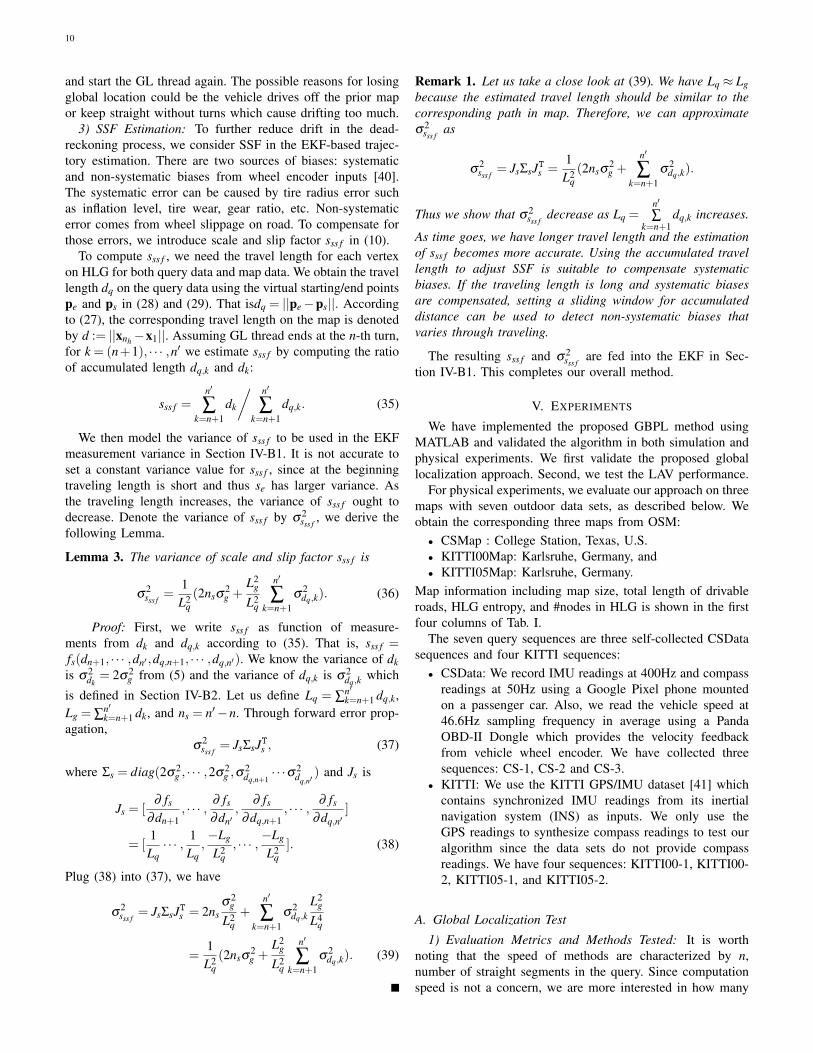
Fig. 12. Scale and slip factor value over time in EKF (10): (a) KITTI dataand (b) CSData. Note the sequences are color coded and are not of the samelength in time.

3) Scale and Slip Factor: Fig. 12 shows the estimated SSFin EKF (i.e. s j in (10)). These results show the effectivenessof LAV in detecting systematic bias in wheel odometry. ForCSData, SSF values are between 1.09 to 1.15 while the SSFvalues from KITTI data are close to 1.00. It is clear that thevehicle velocity from the Panda OBD II dongle contains bias.It tends to underestimated vehicle velocity by about 10%. Thismay be due to incorrect parameters in gear ratio or wheel/tiresize. Also, the fluctuation in SSF in CSData is also large. Thismay also be a result of less accurate GPS values or variabletire inflation status since data is collected at different timesover several months. Nonrigid mounting of the cellphone alsocontributes to the issue. Nevertheless, our GBPL algorithm is

13

0 10 20 30 40 50 60 70

Time(sec)

3

4

5

6

7

8

9va

ria

nce

of

s10-7

KITTI00-1

KITTI00-2

KITTI05-1

KITTI05-2

KITTI05-2KITTI05-1KITTI00-2KITTI00-1

Time(sec)0 10 20 30 40 50 60 70

9

8

7

6

5

4

3

x 10-7

σ

(a)

0 10 20 30 40 50 60 70 80 90

Time(sec)

0

0.2

0.4

0.6

0.8

1

1.2

1.4

1.6

variance�of�s

10-5

CS-1

CS-2

CS-3

1.6

1.4

1.2

1

0.8

0.6

0.4

0.2

00�����10�����20����30�����40����50����60����70�����80����90����

Time(sec)

CS-3CS-2CS-1

x�10-7x�10-5

σ

(b)

Fig. 13. Scale and slip factor variance over time in EKF: (a) KITTI dataand (b) CSData. Note the sequences are color coded and are not of the samelength in time.

robust to these factors and still provides a good localizationresult. We also shows the variance of s j in Fig. 13. Theseresults show σ2

sss fdecreasing as travel length increases as in

Lemma (3).

VI. CONCLUSION AND FUTURE WORK

We reported our GBPL method that did not rely on theperception and recognition of external landmarks to localizerobots/vehicles in urban environments. The proposed methodis designed to be a fallback solution when everything else failsdue to poor lighting conditions or bad weather conditions. Themethod estimated a rudimentry vehicle trajectory computedfrom an IMU, a compass, and a wheel encoder and matched itwith a prior road map. To address the drifting issue in the dead-reckoning process and the fact that the vehicle trajectory maynot overlap with road waypoints on the map, we developeda feature-based Bayesian graph matching where features arelong and straight road segments. GBPL pre-processed mapsinto an HLG which stores all long and straight segments ofroad as nodes to facilitate global localization process. Oncethe map matching is successful, our algorithm tracks vehiclemovement and use the map information to regulate EKF’sdrifting issue. The algorithm was tested in both simulationand physical experiments and results are satisfying.

In the future, we will actively guide the vehicle to maketurns to speed up the localization process. More experimentsare planed which we will work on situations of losing locationand re-localization. We are interested in extending the workto design a multiple vehicle/robot collaborative localizationscheme under ad hoc vehicle-to-vehicle communication frame-work. We will report new results in the future publications.

ACKNOWLEDGMENT

We would like to thank C. Chou, B. Li, S. Yeh, A.Kingery, A. Angert, D. Wang, and S. Xie for their input andcontributions to the NetBot Lab at Texas A&M University.

REFERENCES

[1] H. Cheng, D. Song, A. Angert, B. Li, and J. Yi, “Proprioceptivelocalization assisted by magnetoreception: A minimalist intermittentheading-based approach,” IEEE Robotics and Automation Letters, 2018.

[2] M. A. Brubaker, A. Geiger, and R. Urtasun, “Map-based probabilisticvisual self-localization,” IEEE Transactions on Pattern Analysis andMachine Intelligence, vol. 38, no. 4, pp. 652–665, April 2016.

[3] S. Lowry, N. Sunderhauf, P. Newman, J. J. Leonard, D. Cox, P. Corke,and M. J. Milford, “Visual place recognition: A survey,” IEEE Trans-actions on Robotics, vol. 32, no. 1, pp. 1–19, 2016.

[4] Y. Lu and D. Song, “Visual navigation using heterogeneous landmarksand unsupervised geometric constraints,” in IEEE Transactions onRobotics (T-RO), vol. 31, no. 3, June 2015, pp. 736–749.

[5] D. Hahnel, W. Burgard, D. Fox, and S. Thrun, “An efficient FastSLAMalgorithm for generating maps of large-scale cyclic environments fromraw laser range measurements,” in IEEE/RSJ International Conferenceon Intelligent Robots and Systems (IROS), vol. 1, 2003, pp. 206–211.

[6] W. Hess, D. Kohler, H. Rapp, and D. Andor, “Real-time loop closurein 2d lidar slam,” in Robotics and Automation (ICRA), 2016 IEEEInternational Conference on. IEEE, 2016, pp. 1271–1278.

[7] J. Levinson and S. Thrun, “Robust vehicle localization in urban environ-ments using probabilistic maps,” in Robotics and Automation (ICRA),2010 IEEE International Conference on. IEEE, 2010, pp. 4372–4378.

[8] T. Hunter, P. Abbeel, and A. Bayen, “The path inference filter: model-based low-latency map matching of probe vehicle data,” IEEE Transac-tions on Intelligent Transportation Systems, vol. 15, no. 2, pp. 507–529,2014.

[9] Y. Cui and S. S. Ge, “Autonomous vehicle positioning with gps in urbancanyon environments,” IEEE transactions on robotics and automation,vol. 19, no. 1, pp. 15–25, 2003.

[10] H. Aly, A. Basalamah, and M. Youssef, “Accurate and energy-efficientgps-less outdoor localization,” ACM Trans. Spatial Algorithms Syst.,vol. 3, no. 2, pp. 4:1–4:31, Jul. 2017.

[11] C. Chou, A. Kingery, D. Wang, H. Li, and D. Song, “Encoder-camera-ground penetrating radar tri-sensor mapping for surface and subsurfacetransportation infrastructure inspection,” in 2018 IEEE InternationalConference on Robotics and Automation (ICRA), May 2018, pp. 1452–1457.

[12] M. Li and A. I. Mourikis, “High-precision, consistent EKF-based visual–inertial odometry,” The International Journal of Robotics Research,vol. 32, no. 6, pp. 690–711, 2013.

[13] J. Yi, J. Zhang, D. Song, and S. Jayasuriya, “Imu-based localizationand slip estimation for skid-steered mobile robots,” in Intelligent Robotsand Systems, 2007. IROS 2007. IEEE/RSJ International Conference on.IEEE, 2007, pp. 2845–2850.

[14] L. Paull, S. Saeedi, M. Seto, and H. Li, “Auv navigation and localization:A review,” IEEE Journal of Oceanic Engineering, vol. 39, no. 1, pp.131–149, 2013.

[15] W. Kang and Y. Han, “Smartpdr: Smartphone-based pedestrian deadreckoning for indoor localization,” IEEE Sensors journal, vol. 15, no. 5,pp. 2906–2916, 2014.

[16] I. Constandache, R. R. Choudhury, and I. Rhee, “Compacc: Usingmobile phone compasses and accelerometers for localization,” in IEEEINFOCOM. Citeseer, 2010, pp. 1–9.

[17] G. C. Karras, S. G. Loizou, and K. J. Kyriakopoulos, “On-line stateand parameter estimation of an under-actuated underwater vehicle usinga modified dual unscented kalman filter,” in IEEE/RSJ InternationalConference on Intelligent Robots and Systems(IROS). IEEE, 2010,pp. 4868–4873.

[18] F. Gustafsson, F. Gunnarsson, N. Bergman, U. Forssell, J. Jansson,R. Karlsson, and P.-J. Nordlund, “Particle filters for positioning, nav-igation, and tracking,” IEEE Transactions on signal processing, vol. 50,no. 2, pp. 425–437, 2002.

[19] L. Huang, B. He, and T. Zhang, “An autonomous navigation algorithmfor underwater vehicles based on inertial measurement units and sonar,”in 2010 2nd International Asia Conference on Informatics in Control,Automation and Robotics (CAR 2010), vol. 1. IEEE, 2010, pp. 311–314.

[20] B. Siciliano and O. Khatib, Springer handbook of robotics. Springer,2016.

[21] P. Merriaux, Y. Dupuis, P. Vasseur, and X. Savatier, “Fast and robustvehicle positioning on graph-based representation of drivable maps,” inRobotics and Automation (ICRA), 2015 IEEE International Conferenceon. IEEE, 2015, pp. 2787–2793.

[22] P. Ruchti, B. Steder, M. Ruhnke, and W. Burgard, “Localization onopenstreetmap data using a 3d laser scanner,” in Robotics and Automa-tion (ICRA), 2015 IEEE International Conference on. IEEE, 2015, pp.5260–5265.

[23] R. Jiang, S. Yang, S. S. Ge, H. Wang, and T. H. Lee, “Geometricmap-assisted localization for mobile robots based on uniform-gaussiandistribution,” IEEE Robotics and Automation Letters, vol. 2, no. 2, pp.789–795, 2017.

[24] Y. Jin and Z. Xiang, “Robust localization via turning point filtering withroad map,” in Intelligent Vehicles Symposium (IV), 2016 IEEE. IEEE,2016, pp. 992–997.

14

[25] S. Thrun, W. Burgard, and D. Fox, Probabilistic Robotics. MIT Press,2005.

[26] OpenStreetMap contributors, “Planet dump retrieved fromhttps://planet.osm.org ,” https://www.openstreetmap.org , 2017.

[27] Google Maps contributors, https://www.google.com/maps/ , 2017.[28] M. Quddus and S. Washington, “Shortest path and vehicle trajectory

aided map-matching for low frequency gps data,” Transportation Re-search Part C: Emerging Technologies, vol. 55, pp. 328–339, 2015.

[29] E. Rublee, V. Rabaud, K. Konolige, and G. Bradski, “ORB: An efficientalternative to SIFT or SURF,” in IEEE International Conference onComputer Vision (ICCV), 2011, pp. 2564–2571.

[30] J. Wahlstrom, I. Skog, J. G. P. Rodrigues, P. Handel, and A. Aguiar,“Map-aided dead-reckoning using only measurements of speed,” IEEETransactions on Intelligent Vehicles, vol. 1, no. 3, pp. 244–253, Sep.2016.

[31] B. Yu, L. Dong, D. Xue, H. Zhu, X. Geng, R. Huang, and J. Wang,“A hybrid dead reckoning error correction scheme based on extendedkalman filter and map matching for vehicle self-localization,” Journalof Intelligent Transportation Systems, vol. 23, no. 1, pp. 84–98, 2019.

[32] R. Hartley and A. Zisserman, Multiple view geometry in computer vision.Cambridge university press, 2003.

[33] Y. Bar-Shalom, X. R. Li, and T. Kirubarajan, Estimation with applica-tions to tracking and navigation: theory algorithms and software. JohnWiley & Sons, 2004.

[34] J. Yi, H. Wang, J. Zhang, D. Song, S. Jayasuriya, and J. Liu, “Kinematicmodeling and analysis of skid-steered mobile robots with applicationsto low-cost inertial-measurement-unit-based motion estimation,” IEEETransactions on Robotics, vol. 25, no. 5, pp. 1087–1097, Oct 2009.

[35] H.-M. Cheng and D. Song, “Localization in inconsistent wifi environ-ments,” in The International Symposium on Robotics Research (ISRR),Puerto Varas, Chile, 2017.

[36] N. Otsu, “A threshold selection method from gray-level histograms,”IEEE transactions on systems, man, and cybernetics, vol. 9, no. 1, pp.62–66, 1979.

[37] R. A. Kronmal and A. V. Peterson Jr, “On the alias method forgenerating random variables from a discrete distribution,” The AmericanStatistician, vol. 33, no. 4, pp. 214–218, 1979.

[38] G. Boeing, “Urban spatial order: Street network ori-entation, configuration, and entropy.” [Online]. Available:http://arxiv.org/abs/1808.00600v2

[39] N. Mohajeri and A. Gudmundsson, “The evolution and complexity ofurban street networks,” Geographical Analysis, vol. 46, no. 4, pp. 345–367, 2014.

[40] J. Borenstein and L. Feng, “Correction of systematic odometry errorsin mobile robots,” in Proceedings 1995 IEEE/RSJ International Confer-ence on Intelligent Robots and Systems. Human Robot Interaction andCooperative Robots, vol. 3. IEEE, 1995, pp. 569–574.

[41] A. Geiger, P. Lenz, and R. Urtasun, “Are we ready for autonomousdriving? the kitti vision benchmark suite,” in Computer Vision andPattern Recognition (CVPR), 2012 IEEE Conference on. IEEE, 2012,pp. 3354–3361.

Hsin-Min Cheng received the B.S. degree fromthe Department of Electronics Engineering, NationalChiao Tung University, Hsinchu, Taiwan, in 2010,and the M.S. degree from the Department of Elec-tronics Engineering, National Chiao Tung Univer-sity, Hsinchu, Taiwan, in 2012. She is currentlyworking toward the Ph.D. degree at the Departmentof Computer Science and Engineering, Texas AMUniversity, College Station, TX, USA.

Her research interests include robot perception,sensor fusion, and localization.

Dezhen Song (S’02-M’04-SM’09) received thePh.D. degree in industrial engineering and operationsresearch from University of California, Berkeley,CA, US, in 2004.

He is a Professor with Department of ComputerScience and Engineering, Texas A&M University,College Station, TX, USA. His research interestsinclude networked robots, multi-modal perception,computer vision, and stochastic modeling.

Dr. Song received the Kayamori Best Paper Awardof the 2005 IEEE International Conference on

Robotics and Automation (with J. Yi and S. Ding). He received NSF FacultyEarly Career Development (CAREER) Award in 2007. From 2008 to 2012,Song was an associate editor of IEEE Transactions on Robotics. From 2010to 2014, Song was an Associate Editor of IEEE Transactions on AutomationScience and Engineering. From 2017 to 2020, he was a Senior Editor forIEEE Robotics and Automation Letters (RA-L).