hydraulic fracturing in unconventional shale gas reservoirs · 3 simulation of hydraulic fracturing...
TRANSCRIPT
Hydraulic fracturing in unconventional shale gas
reservoirs
Dr.-Ing. Johannes Will,Dynardo GmbH, Weimar, Germany
2 Simulation of Hydraulic Fracturing
CAE-Consulting
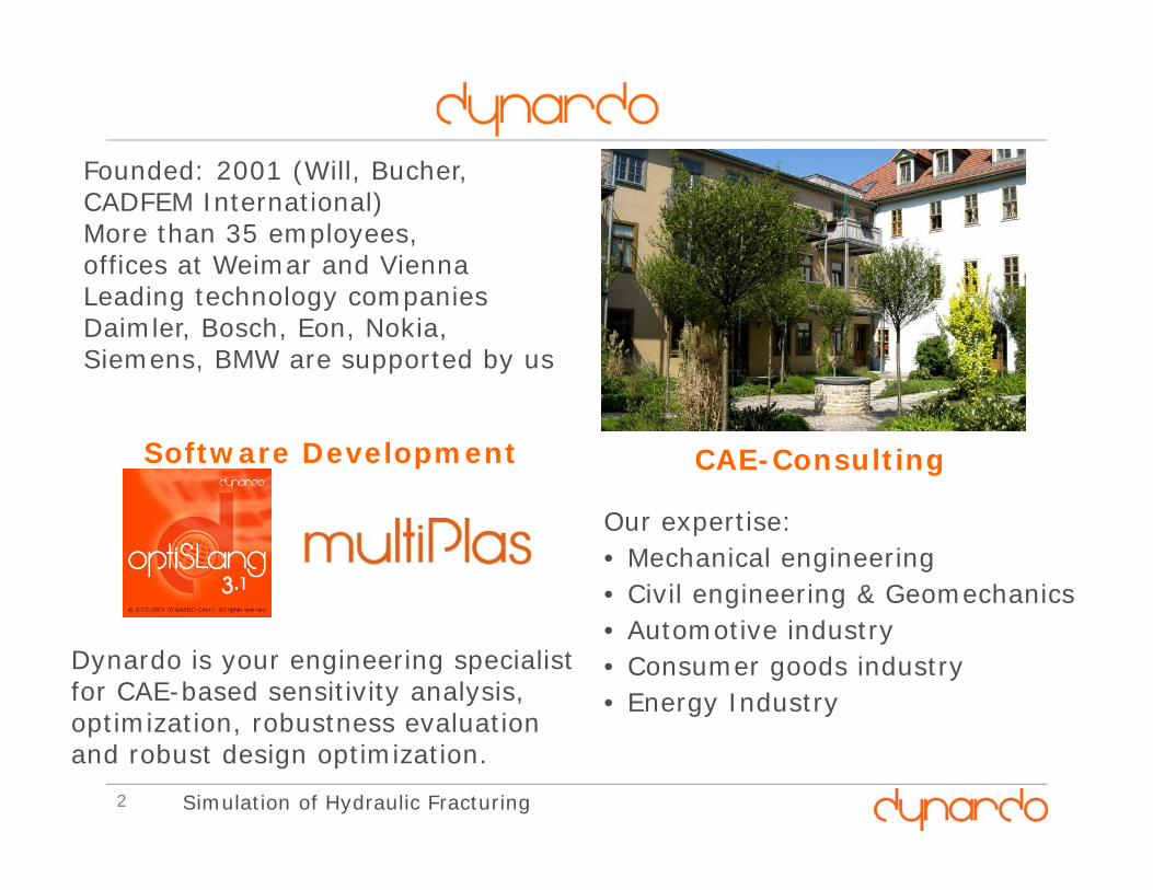
Our expertise: • Mechanical engineering• Civil engineering & Geomechanics• Automotive industry• Consumer goods industry• Energy Industry
Software Development
Dynardo is your engineering specialist for CAE-based sensitivity analysis, optimization, robustness evaluation and robust design optimization.
Founded: 2001 (Will, Bucher, CADFEM International)More than 35 employees, offices at Weimar and ViennaLeading technology companies Daimler, Bosch, Eon, Nokia, Siemens, BMW are supported by us
3 Simulation of Hydraulic Fracturing
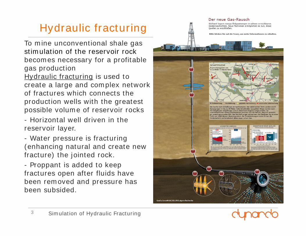
To mine unconventional shale gas stimulation of the reservoir rock becomes necessary for a profitable gas productionHydraulic fracturing is used to create a large and complex network of fractures which connects the production wells with the greatest possible volume of reservoir rocks- Horizontal well driven in the reservoir layer. - Water pressure is fracturing (enhancing natural and create new fracture) the jointed rock.- Proppant is added to keep fractures open after fluids have been removed and pressure has been subsided.
Hydraulic fracturing
Simulation of hydraulic fracturing of jointed rock
Dr.-Ing. Johannes Will,Dynardo GmbH, Weimar, Germany
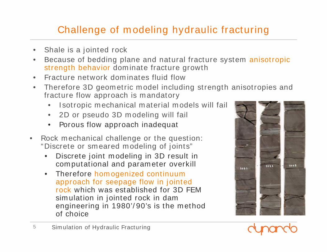
Challenge of modeling hydraulic fracturing
• Shale is a jointed rock• Because of bedding plane and natural fracture system anisotropic
strength behavior dominate fracture growth• Fracture network dominates fluid flow• Therefore 3D geometric model including strength anisotropies and
fracture flow approach is mandatory• Isotropic mechanical material models will fail• 2D or pseudo 3D modeling will fail• Porous flow approach inadequat
• Rock mechanical challenge or the question: “Discrete or smeared modeling of joints”• Discrete joint modeling in 3D result in
computational and parameter overkill• Therefore homogenized continuum
approach for seepage flow in jointed rock which was established for 3D FEM simulation in jointed rock in dam engineering in 1980’/90’s is the method of choice
Simulation of Hydraulic Fracturing5
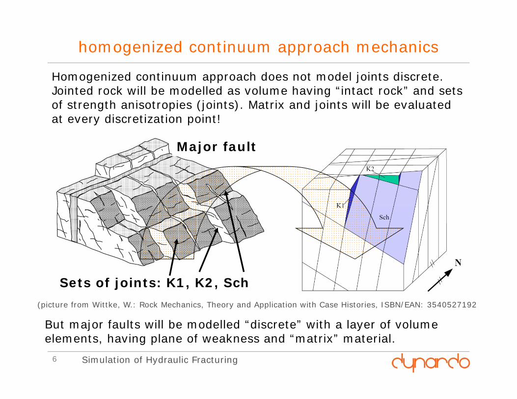
homogenized continuum approach mechanics
Major fault
Sets of joints: K1, K2, Sch
But major faults will be modelled “discrete” with a layer of volume elements, having plane of weakness and “matrix” material.
(picture from Wittke, W.: Rock Mechanics, Theory and Application with Case Histories, ISBN/EAN: 3540527192
Homogenized continuum approach does not model joints discrete. Jointed rock will be modelled as volume having “intact rock” and sets of strength anisotropies (joints). Matrix and joints will be evaluated at every discretization point!
Simulation of Hydraulic Fracturing6
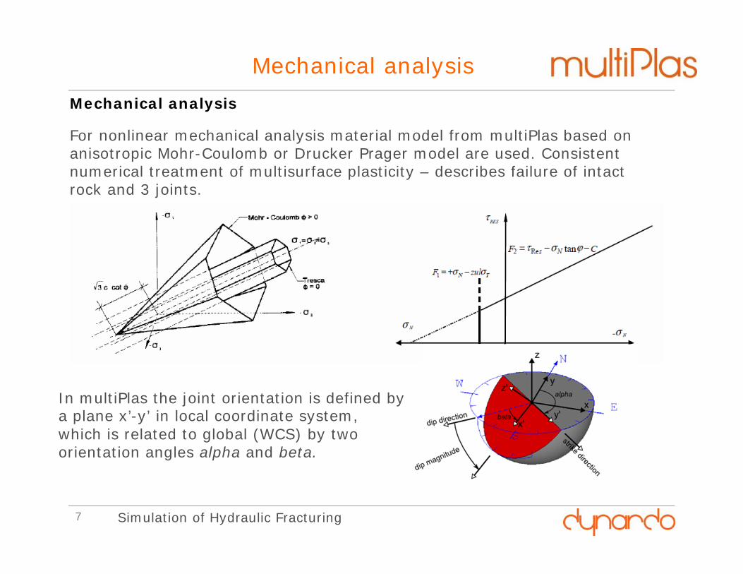
For nonlinear mechanical analysis material model from multiPlas based on anisotropic Mohr-Coulomb or Drucker Prager model are used. Consistent numerical treatment of multisurface plasticity – describes failure of intact rock and 3 joints.
Mechanical analysis
Mechanical analysis
In multiPlas the joint orientation is defined by a plane x’-y’ in local coordinate system, which is related to global (WCS) by two orientation angles alpha and beta.
Simulation of Hydraulic Fracturing7
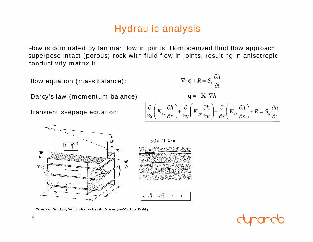
Hydraulic analysis
8
Flow is dominated by laminar flow in joints. Homogenized fluid flow approach superpose intact (porous) rock with fluid flow in joints, resulting in anisotropic conductivity matrix K
thSR s
qflow equation (mass balance):
Darcy’s law (momentum balance): h Kq
thSR
zhK
zyhK
yxhK
x szzyyxx
transient seepage equation:
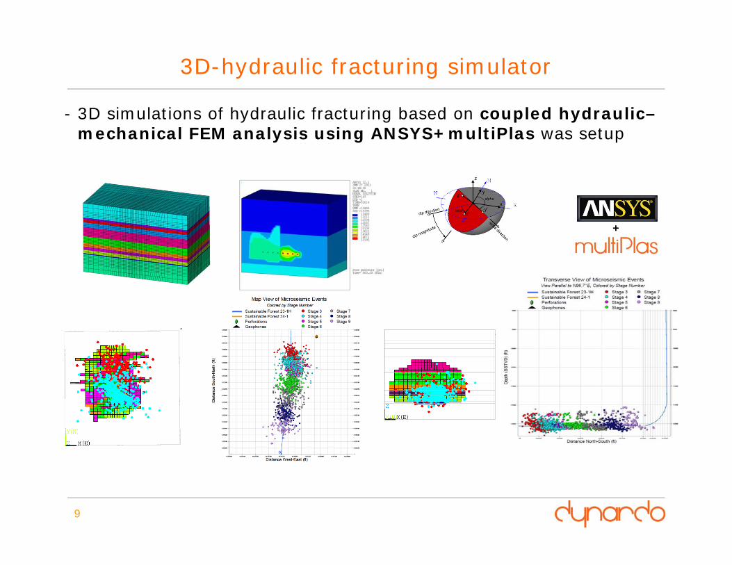
3D-hydraulic fracturing simulator
9
+
- 3D simulations of hydraulic fracturing based on coupled hydraulic–mechanical FEM analysis using ANSYS+multiPlas was setup
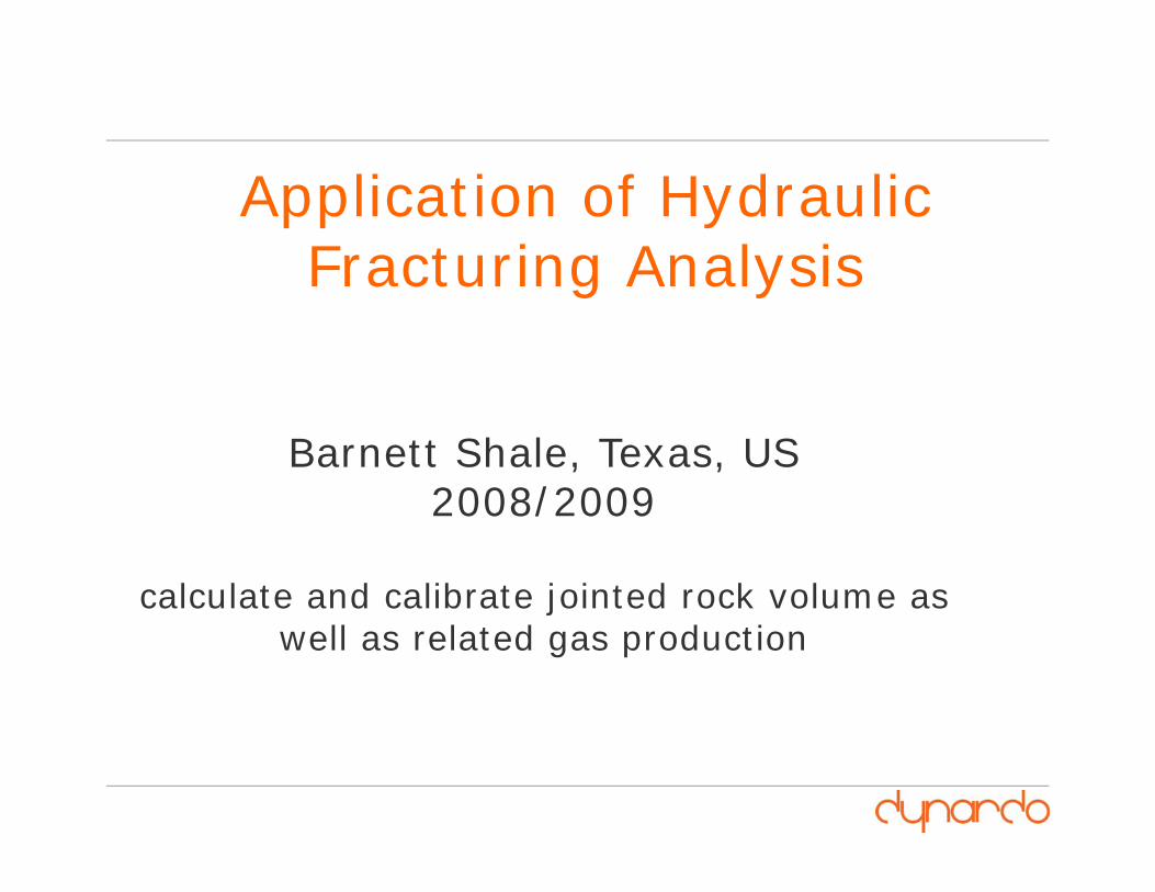
Application of Hydraulic Fracturing Analysis
Barnett Shale, Texas, US2008/2009
calculate and calibrate jointed rock volume as well as related gas production
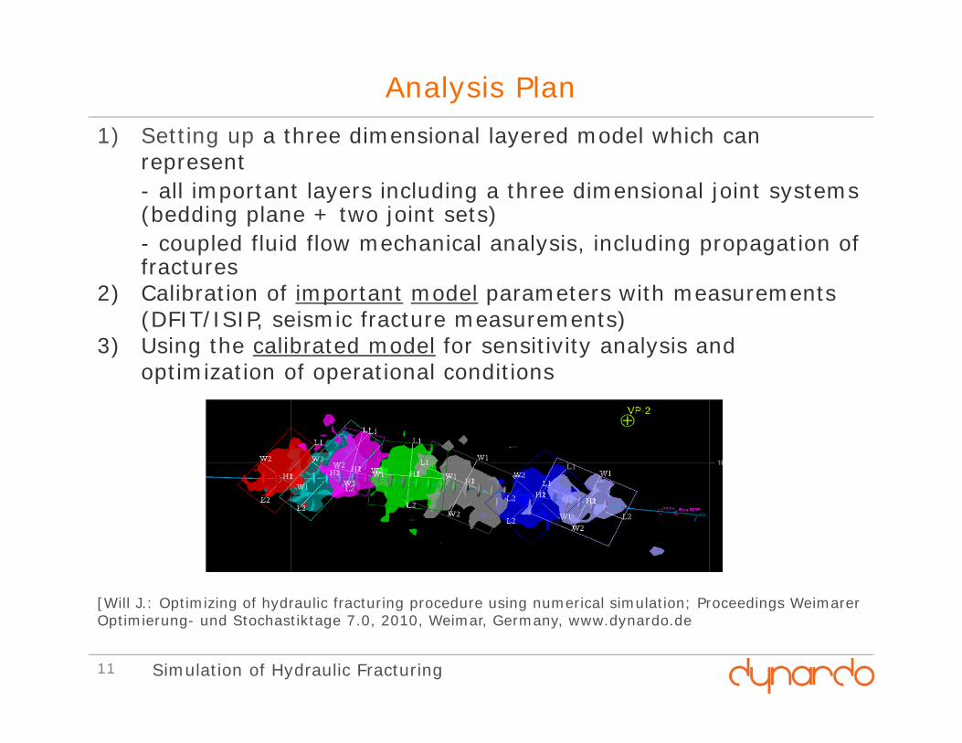
Analysis Plan1) Setting up a three dimensional layered model which can
represent- all important layers including a three dimensional joint systems (bedding plane + two joint sets)- coupled fluid flow mechanical analysis, including propagation of fractures
2) Calibration of important model parameters with measurements (DFIT/ISIP, seismic fracture measurements)
3) Using the calibrated model for sensitivity analysis and optimization of operational conditions
Simulation of Hydraulic Fracturing11
[Will J.: Optimizing of hydraulic fracturing procedure using numerical simulation; Proceedings Weimarer Optimierung- und Stochastiktage 7.0, 2010, Weimar, Germany, www.dynardo.de
12 Simulation of Hydraulic Fracturing
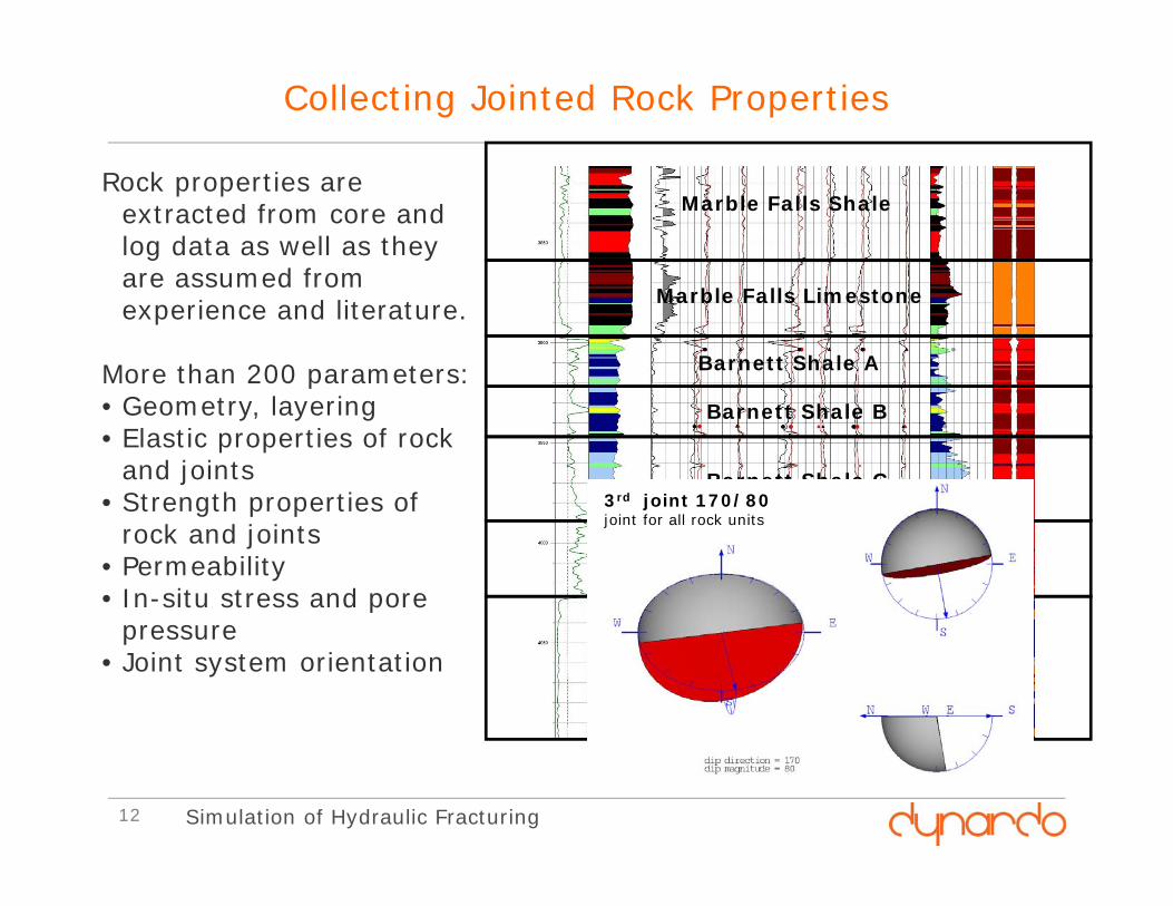
Collecting Jointed Rock Properties
Marble Falls Shale
Marble Falls Limestone
Barnett Shale A
Barnett Shale B
Barnett Shale C
Barnett Shale D
Ellenburger
Rock properties are extracted from core and log data as well as they are assumed from experience and literature.
More than 200 parameters:• Geometry, layering• Elastic properties of rock
and joints• Strength properties of
rock and joints• Permeability • In-situ stress and pore
pressure• Joint system orientation
3rd joint 170/80joint for all rock units
Simulation of Hydraulic Fracturing
Parametric model setup and calibration
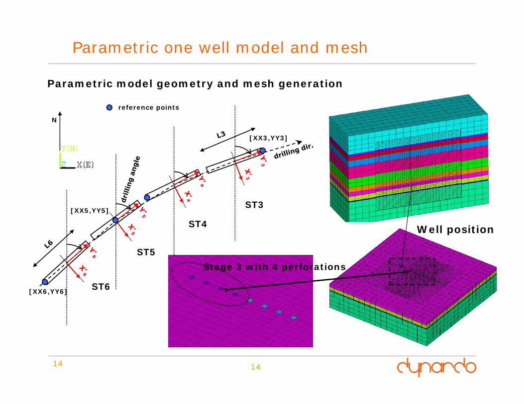
Parametric one well model and mesh
14 14
Parametric model geometry and mesh generation
N
reference points
[XX6,YY6]
[XX5,YY5]
[XX3,YY3]
ST6
ST5
ST4
ST3
Stage 3 with 4 perforations
Well position
15 ECF 18 Simulation of Hydraulic Fracturing
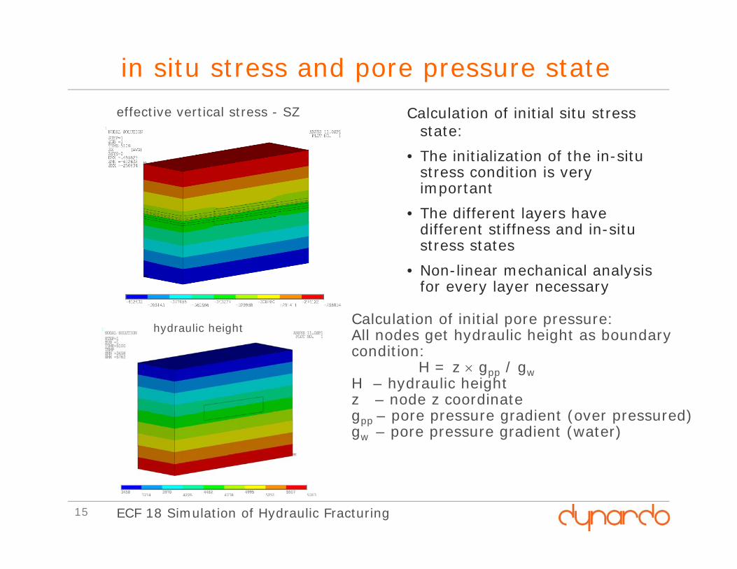
in situ stress and pore pressure stateCalculation of initial situ stress
state:• The initialization of the in-situ
stress condition is very important
• The different layers have different stiffness and in-situ stress states
• Non-linear mechanical analysis for every layer necessary
effective vertical stress - SZ
Calculation of initial pore pressure:All nodes get hydraulic height as boundary condition:
H = z gpp / gwH – hydraulic heightz – node z coordinategpp – pore pressure gradient (over pressured)gw – pore pressure gradient (water)
hydraulic height
16 ECF 18 Simulation of Hydraulic Fracturing
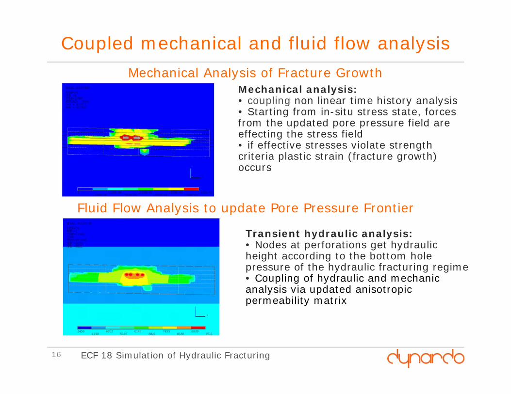
Coupled mechanical and fluid flow analysis
Mechanical analysis:• coupling non linear time history analysis• Starting from in-situ stress state, forces from the updated pore pressure field are effecting the stress field• if effective stresses violate strength criteria plastic strain (fracture growth) occurs
Mechanical Analysis of Fracture Growth
Transient hydraulic analysis:• Nodes at perforations get hydraulic height according to the bottom hole pressure of the hydraulic fracturing regime• Coupling of hydraulic and mechanic analysis via updated anisotropic permeability matrix
Fluid Flow Analysis to update Pore Pressure Frontier
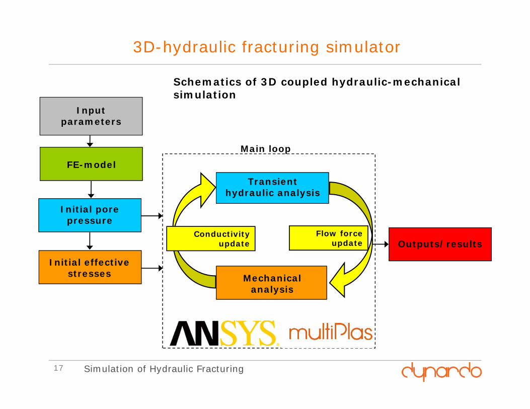
3D-hydraulic fracturing simulator
Input parameters
FE-model
Initial pore pressure
Initial effective stresses Mechanical
analysis
Transient hydraulic analysis
Schematics of 3D coupled hydraulic-mechanical simulation
Outputs/results
Main loop
Flow force update
Conductivity update
Simulation of Hydraulic Fracturing17
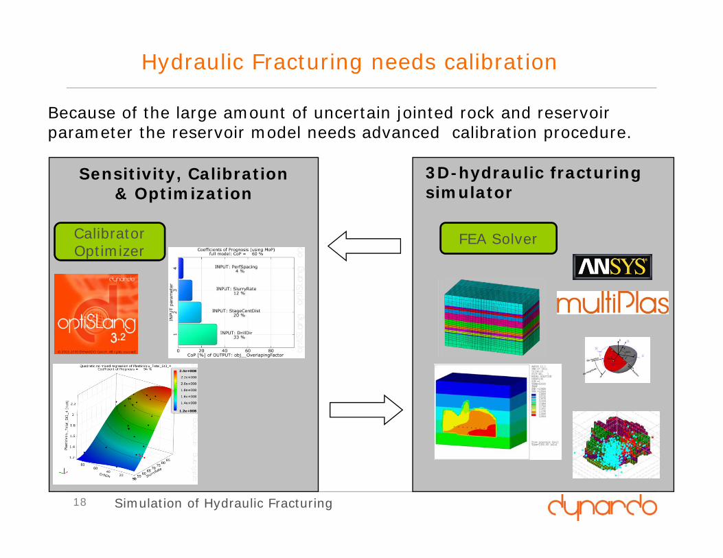
Hydraulic Fracturing needs calibration
Sensitivity, Calibration & Optimization
3D-hydraulic fracturing simulator
FEA SolverCalibrator Optimizer
Simulation of Hydraulic Fracturing18
Because of the large amount of uncertain jointed rock and reservoir parameter the reservoir model needs advanced calibration procedure.
19 Simulation of Hydraulic Fracturing
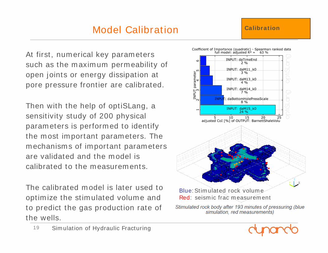
Model Calibration Calibration
At first, numerical key parameters such as the maximum permeability of open joints or energy dissipation at pore pressure frontier are calibrated.
Then with the help of optiSLang, a sensitivity study of 200 physical parameters is performed to identify the most important parameters. The mechanisms of important parameters are validated and the model is calibrated to the measurements.
The calibrated model is later used to optimize the stimulated volume and to predict the gas production rate of the wells.
Blue:Stimulated rock volumeRed: seismic frac measurement
Modeling of Hydraulic Fracturing
Using the Calibrated Model for Prediction and Optimization
21 Simulation of Hydraulic Fracturing
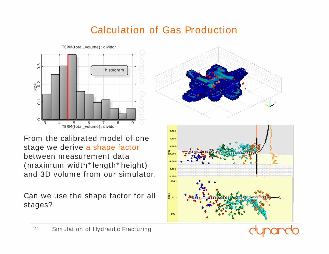
Calculation of Gas Production
From the calibrated model of one stage we derive a shape factorbetween measurement data (maximum width*length*height) and 3D volume from our simulator.
Can we use the shape factor for all stages?
22 Simulation of Hydraulic Fracturing
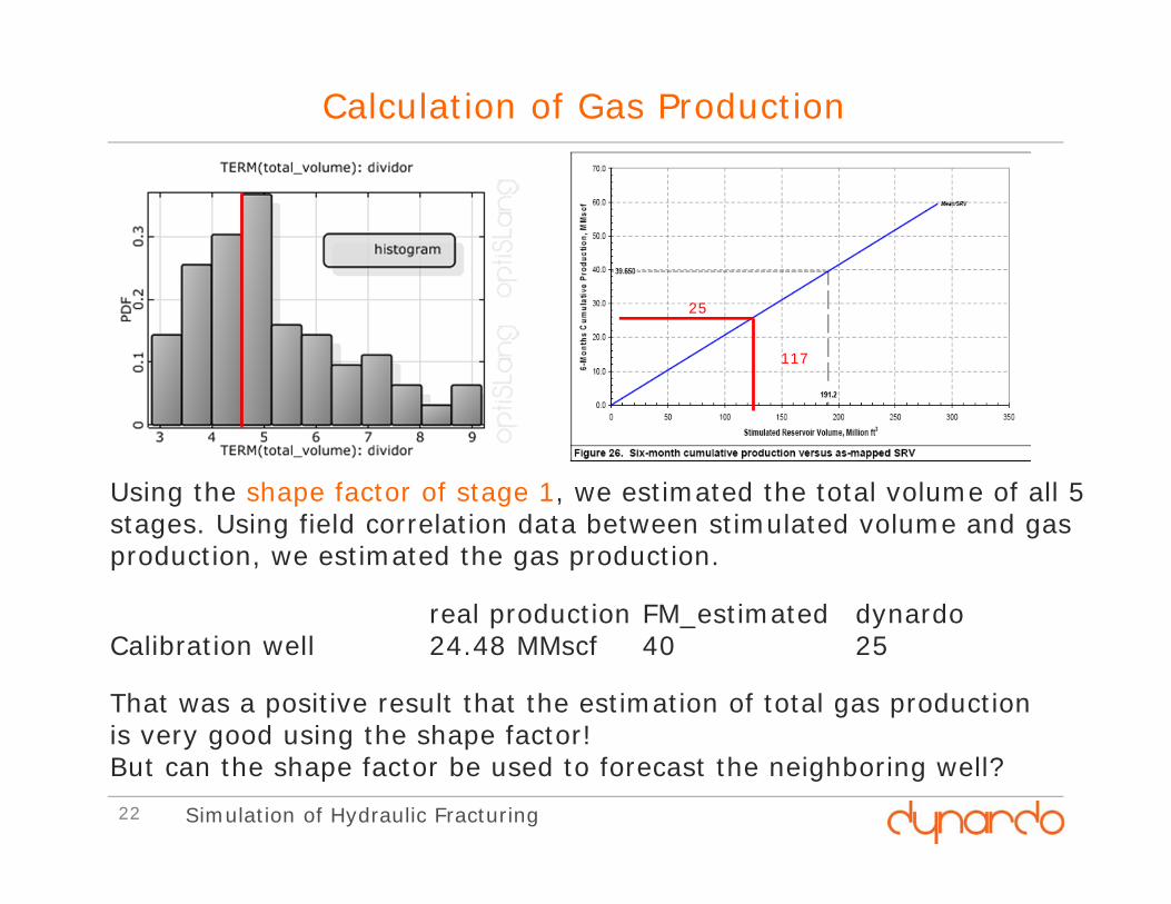
Calculation of Gas Production
Using the shape factor of stage 1, we estimated the total volume of all 5 stages. Using field correlation data between stimulated volume and gas production, we estimated the gas production.
117
25
real production FM_estimated dynardoCalibration well 24.48 MMscf 40 25
That was a positive result that the estimation of total gas production is very good using the shape factor! But can the shape factor be used to forecast the neighboring well?
23 Simulation of Hydraulic Fracturing
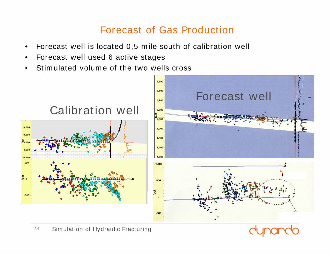
Forecast of Gas Production• Forecast well is located 0,5 mile south of calibration well• Forecast well used 6 active stages • Stimulated volume of the two wells cross
Calibration wellForecast well
24 Simulation of Hydraulic Fracturing
Forecast of Gas Production
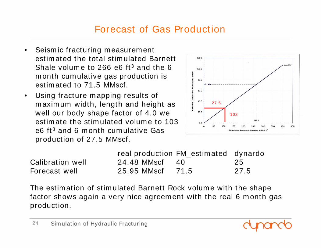
real production FM_estimated dynardoCalibration well 24.48 MMscf 40 25Forecast well 25.95 MMscf 71.5 27.5
The estimation of stimulated Barnett Rock volume with the shape factor shows again a very nice agreement with the real 6 month gas production.
• Seismic fracturing measurement estimated the total stimulated Barnett Shale volume to 266 e6 ft3 and the 6 month cumulative gas production is estimated to 71.5 MMscf.
• Using fracture mapping results of maximum width, length and height as well our body shape factor of 4.0 we estimate the stimulated volume to 103 e6 ft3 and 6 month cumulative Gas production of 27.5 MMscf.
103
27.5
25 Simulation of Hydraulic Fracturing
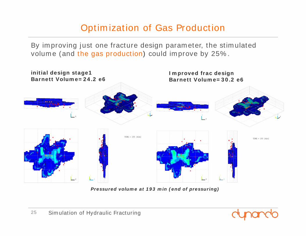
Pressured volume at 193 min (end of pressuring)
initial design stage1Barnett Volume=24.2 e6
Improved frac designBarnett Volume=30.2 e6
By improving just one fracture design parameter, the stimulated volume (and the gas production) could improve by 25%.
Optimization of Gas Production
Application of Hydraulic Fracturing Analysis
other Reservoirs, US2010/2011
calculate and calibrate joint network creation including stage and well interaction
27 Simulation of Hydraulic Fracturing
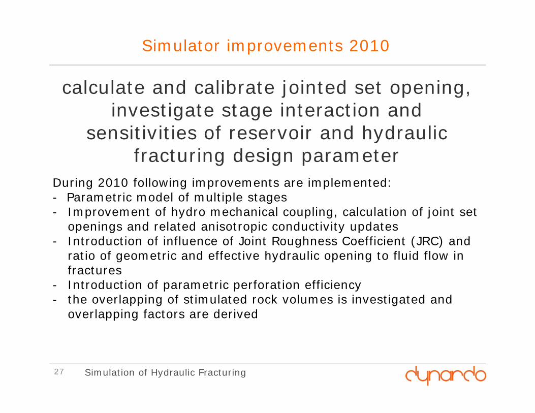
Simulator improvements 2010
During 2010 following improvements are implemented:- Parametric model of multiple stages- Improvement of hydro mechanical coupling, calculation of joint set
openings and related anisotropic conductivity updates - Introduction of influence of Joint Roughness Coefficient (JRC) and
ratio of geometric and effective hydraulic opening to fluid flow in fractures
- Introduction of parametric perforation efficiency- the overlapping of stimulated rock volumes is investigated and
overlapping factors are derived
calculate and calibrate jointed set opening, investigate stage interaction and
sensitivities of reservoir and hydraulic fracturing design parameter
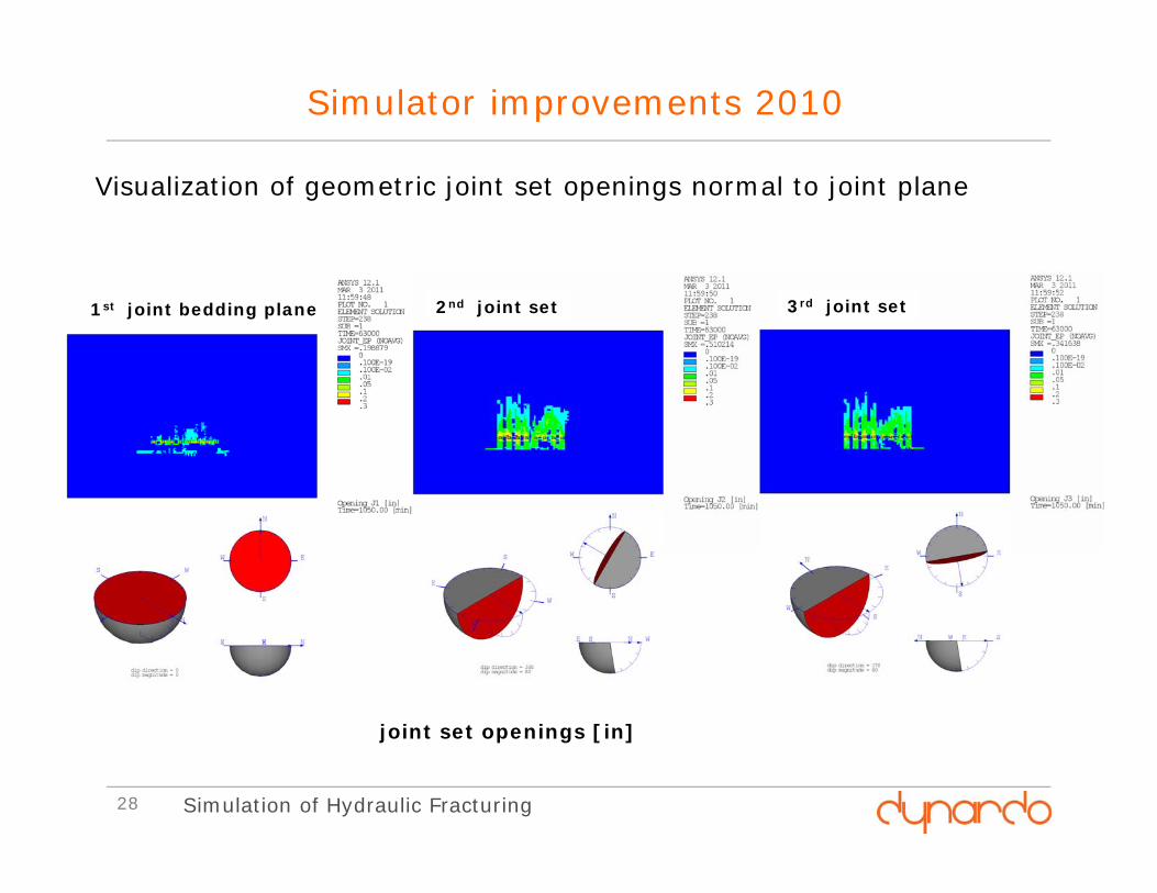
Visualization of geometric joint set openings normal to joint plane
3rd joint set2nd joint set1st joint bedding plane
joint set openings [in]
Simulator improvements 2010
Simulation of Hydraulic Fracturing28
29 Simulation of Hydraulic Fracturing
Simulator improvements 2011
Industrial projects (short term)- Improvement of parametric to model and calculate multiple stages
at multiple well to investigate well interaction and re-stimulation- Introduction of dilatancy functions and non local material models
to improve accuracy of permeability update
Funded projects (mid term)- Speed up simulation process and minimize memory requirements- Extraction of most probable network of joints, export network to
reservoir simulators and CFD codes- Implementation of stress dependent conductivity decline to run
flow back and production
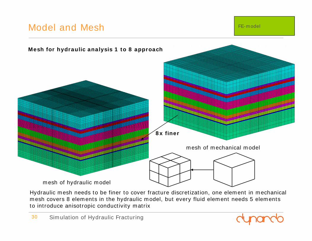
Model and Mesh
30
Hydraulic mesh needs to be finer to cover fracture discretization, one element in mechanical mesh covers 8 elements in the hydraulic model, but every fluid element needs 5 elements to introduce anisotropic conductivity matrix
8x finer
Mesh for hydraulic analysis 1 to 8 approach
FE-model
mesh of mechanical model
mesh of hydraulic model
Simulation of Hydraulic Fracturing
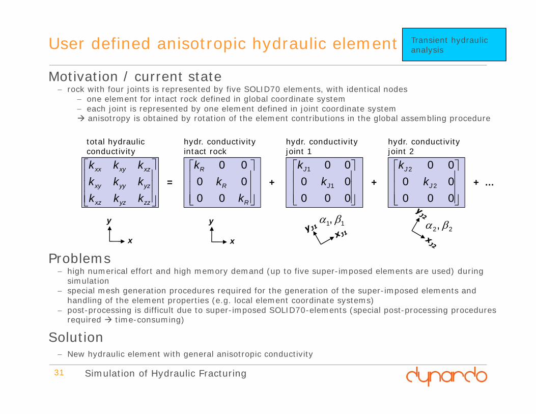
User defined anisotropic hydraulic element
31
Motivation / current state rock with four joints is represented by five SOLID70 elements, with identical nodes
one element for intact rock defined in global coordinate system each joint is represented by one element defined in joint coordinate system anisotropy is obtained by rotation of the element contributions in the global assembling procedure
Transient hydraulic analysis
= + + + …
zzyzxz
yzyyxy
xzxyxx
kkkkkkkkk
x
y
total hydraulic conductivity
R
R
R
kk
k
000000
x
y
hydr. conductivity intact rock
0000000
1
1
J
J
kk
11,
hydr. conductivity joint 1
0000000
2
2
J
J
kk
22,
hydr. conductivity joint 2
Problems high numerical effort and high memory demand (up to five super-imposed elements are used) during
simulation special mesh generation procedures required for the generation of the super-imposed elements and
handling of the element properties (e.g. local element coordinate systems) post-processing is difficult due to super-imposed SOLID70-elements (special post-processing procedures
required time-consuming)
Solution New hydraulic element with general anisotropic conductivity
Simulation of Hydraulic Fracturing
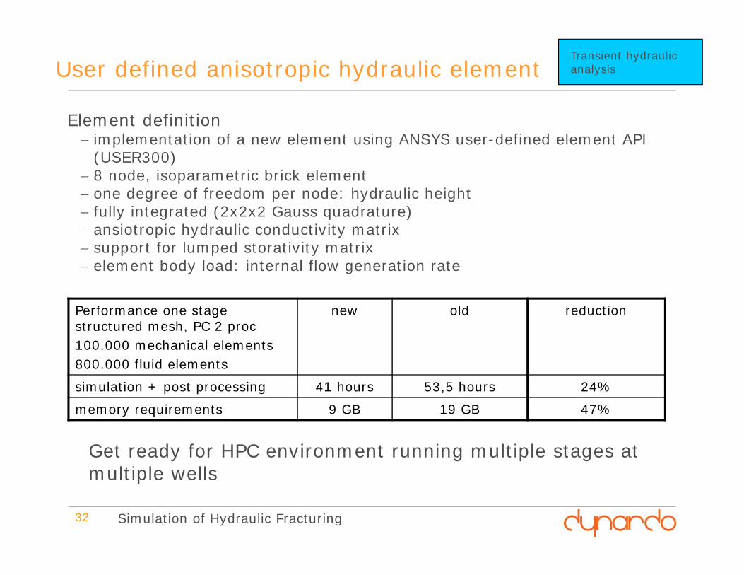
User defined anisotropic hydraulic element
32
Element definition implementation of a new element using ANSYS user-defined element API
(USER300) 8 node, isoparametric brick element one degree of freedom per node: hydraulic height fully integrated (2x2x2 Gauss quadrature) ansiotropic hydraulic conductivity matrix support for lumped storativity matrix element body load: internal flow generation rate
Transient hydraulic analysis
Performance one stage structured mesh, PC 2 proc100.000 mechanical elements800.000 fluid elements
new old reduction
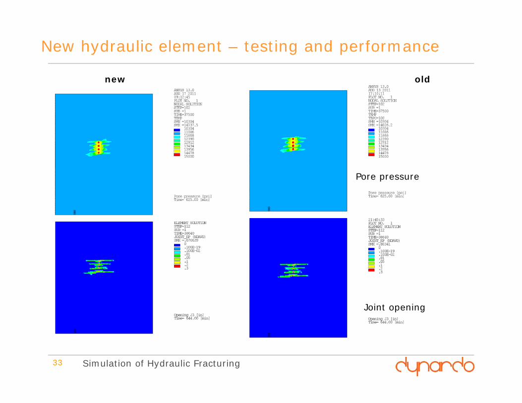
simulation + post processing 41 hours 53,5 hours 24%
memory requirements 9 GB 19 GB 47%
Simulation of Hydraulic Fracturing
Get ready for HPC environment running multiple stages at multiple wells
new old
New hydraulic element – testing and performance
Simulation of Hydraulic Fracturing
Pore pressure
Joint opening
33
www.dynardo.de
Please visit our homepage and contact us for more information!Simulation of Hydraulic Fracturing