hydroacoustic analysis of the effects of a tidal power

The University of MaineDigitalCommons@UMaine

Electronic Theses and Dissertations Fogler Library

12-2016

Hydroacoustic Analysis of the Effects of a TidalPower Turbine on FishesHaley ViehmanUniversity of Maine - Main, [email protected]

Follow this and additional works at: http://digitalcommons.library.umaine.edu/etd

Part of the Marine Biology Commons

This Open-Access Dissertation is brought to you for free and open access by DigitalCommons@UMaine. It has been accepted for inclusion inElectronic Theses and Dissertations by an authorized administrator of DigitalCommons@UMaine.

Recommended CitationViehman, Haley, "Hydroacoustic Analysis of the Effects of a Tidal Power Turbine on Fishes" (2016). Electronic Theses and Dissertations.2546.http://digitalcommons.library.umaine.edu/etd/2546

http://digitalcommons.library.umaine.edu?utm_source=digitalcommons.library.umaine.edu%2Fetd%2F2546&utm_medium=PDF&utm_campaign=PDFCoverPages

http://digitalcommons.library.umaine.edu/etd?utm_source=digitalcommons.library.umaine.edu%2Fetd%2F2546&utm_medium=PDF&utm_campaign=PDFCoverPages

http://digitalcommons.library.umaine.edu/fogler?utm_source=digitalcommons.library.umaine.edu%2Fetd%2F2546&utm_medium=PDF&utm_campaign=PDFCoverPages

http://digitalcommons.library.umaine.edu/etd?utm_source=digitalcommons.library.umaine.edu%2Fetd%2F2546&utm_medium=PDF&utm_campaign=PDFCoverPages

http://network.bepress.com/hgg/discipline/1126?utm_source=digitalcommons.library.umaine.edu%2Fetd%2F2546&utm_medium=PDF&utm_campaign=PDFCoverPages

http://digitalcommons.library.umaine.edu/etd/2546?utm_source=digitalcommons.library.umaine.edu%2Fetd%2F2546&utm_medium=PDF&utm_campaign=PDFCoverPages

HYDROACOUSTIC ANALYSIS OF THE EFFECTS

OF A TIDAL POWER TURBINE ON FISHES

By

Haley A. Viehman

B.S. Cornell University, 2009

M.S. University of Maine, 2012

A DISSERTATION

Submitted in Partial Fulfillment of the

Requirements for the Degree of

Doctor of Philosophy

(Interdisciplinary in Engineering and the Natural Sciences)

The Graduate School

The University of Maine

December 2016

Advisory Committee:

Gayle B. Zydlewski, Associate Professor of Marine Science, Co-advisor

Michael Peterson, Professor of Mechanical Engineering, Co-advisor

Huijie Xue, Professor of Marine Science

William Halteman, Professor Emeritus of Mathematics and Statistics

Donald Degan, President of Aquacoustics, Inc.

DISSERTATION ACCEPTANCE STATEMENT

On behalf of the Graduate Committee for Haley Viehman, I affirm that this

manuscript is the final and accepted dissertation. Signatures of all committee members

are on file with the Graduate School at the University of Maine, 42 Stodder Hall, Orono,

Maine.

ski, Associate Professor of Marine Science------ ^Date

Dr. Michael Peterson, Professor of Mechanical Engineering— * -Date

LIBRARY RIGHTS STATEMENT

In presenting this dissertation in partial fulfillment of the requirements for an

advanced degree at the University of Maine, I agree that the Library shall make it freely

available for inspection. I further agree that permission for “fair use” copying of this

dissertation for scholarly purposes may be granted by the Librarian. It is understood that

any copying or publication of this dissertation for financial gain shall not be allowed

without my written permission.

Signature:

Date:

HYDROACOUSTIC ANALYSIS OF THE EFFECTS

OF A TIDAL POWER TURBINE ON FISHES

By Haley Viehman

Dissertation Co-Advisor: Dr. Gayle Zydlewski

Dissertation Co-Advisor: Dr. Michael Peterson

An Abstract of the Dissertation Presented

in Partial Fulfillment of the Requirements for the

Degree of Doctor of Philosophy

(Interdisciplinary in Engineering and the Natural Sciences)

December 2016

Tidal currents help shape coastal marine environments and are essential in the life

cycles of many marine and diadromous fishes. Areas with strong tidal currents are also

targeted by humans for energy extraction via marine hydrokinetic (MHK) turbines. The

effects of these devices on fishes are difficult to predict because the presence and

behavior of fish within fast tidal currents is largely unstudied. Based at a tidal energy site

in Cobscook Bay, Maine, this work sought to characterize nearfield fish responses to an

MHK device, to describe the natural presence of fish at the site, and to provide guidance

for monitoring MHK device effects in these highly dynamic environments. A bottom-

mounted hydroacoustic echosounder monitored the behavior of fish 7-14 m away from

the static MHK device for several weeks. Fish mainly moved with the current, but those

approaching the device showed signs of avoidance via slight divergence from the main

current direction. The same echosounder was used to collect a two-year time series of

hourly fish passage rate at turbine depth after device removal. Fish passage rate, and

therefore potential encounter rate with the turbine, varied greatly over multiple time

scales, and reflected the dominant environmental patterns, including tidal, diel, lunar, and

seasonal cycles. When simulated discrete surveys of fish presence were informed by

these cyclic components (e.g., 24-hr surveys occurring at the same lunar stage throughout

the year), variation in the results was reduced. This approach to discrete survey design at

tidal energy sites could increase the power of before-after-control-impact comparisons to

detect device effects without requiring expensive continuous or high-frequency sampling

over the long-term. Additionally, deconvolution techniques applied to narrow-angle (7°)

single beam data yielded target strength distributions comparable to corresponding split

beam data. Depending on study aims, the use of single beam echosounders could

substantially reduce study costs while supplying sufficient information on device effects

for use in management decisions. Results from Cobscook Bay are likely applicable to

other study sites with similar environmental forcing, but study designs and results should

be considered in the context of each site’s fish assemblage.

iii

ACKNOWLEDGEMENTS

I would like to thank my advisor, Dr. Gayle Zydlewski, for the opportunity to

work on this project throughout my graduate carreer. Without her continuous

enthusiasm, guidance, and patience, this work would not be possible. I also thank my

advisory committee, Michael Peterson, William Halteman, Huijie Xue, and Donald

Degan, for their continuous support and contributions to this work.

I also thank all others who assisted in field work or data analysis, including the

other members of the Gayle Zydlewski lab: Dr. James McCleave, Garrett Staines, Jeffrey

Vieser, Kevin Lachapelle, Dr. Haixue Shen, Megan Altenritter, Dr. Matthew Altenritter,

Catherine Johnston, Aurélie Daroux, and Constantin Scherelis. Thank you also to the

members of the Maine Tidal Power Initiative for their insights and interest in our various

projects over the past seven years.

The employees of Ocean Renewable Power Company were essential to all of our

work in Cobscook Bay, generously contributing time and resources to all aspects of our

field work. Thanks also to Chris Bartlet of Maine Sea Grant, who assisted in field work

and was instrumental in connecting us with the communities of Eastport and Lubec.

Briony Hutton and Toby Jarvis of Echoview® were also incredibly helpful as I developed

the processing techniques for a wide variety of hydroacoustic data.

None of this work could have taken place without the knowledge and skill of

Captain Butch Harris and his crew, and I thank them for their boundless generosity and

understanding through many long hours of acoustic surveys, and for the countless times

they went out of their way to assist us during this process.

iv

Funding was provided by the United States Department of Energy project #DE-

EE0003647 and #DE-EE0006384, and Maine Sea Grant project #NA10OAR4170081.

Finally, I wish to thank my friends and family for their endless love and support.

v

TABLE OF CONTENTS

ACKNOWLEDGEMENTS ............................................................................................... iii

LIST OF TABLES ............................................................................................................. ix

LIST OF FIGURES ............................................................................................................ x

1. FISH BEHAVIOR NEAR A STATIC TIDAL ENERGY DEVICE............................. 1

1.1 Abstract ............................................................................................................. 1

1.2 Introduction ....................................................................................................... 2

1.3 Methods............................................................................................................. 6

1.3.1 Data processing ...................................................................................... 10

1.3.2 Data analysis .......................................................................................... 17

1.4 Results ............................................................................................................. 19

1.5 Discussion ....................................................................................................... 25

2. POTENTIAL OF SINGLE BEAM ECHOSOUNDERS FOR

ASSESSING FISH AT TIDAL ENERGY SITES ..................................................... 33

2.1 Abstract ........................................................................................................... 33

2.2 Introduction ..................................................................................................... 34

2.3 Methods........................................................................................................... 39

2.3.1 Echosounder calibration......................................................................... 41

2.3.2 Data processing ...................................................................................... 42

2.3.3 Deconvolution ........................................................................................ 44

2.3.4 Beam pattern PDF .................................................................................. 46

2.3.5 Fish echo PDF ........................................................................................ 47

2.3.6 Assessment of deconvolution accuracy ................................................. 49

vi

2.4 Results ............................................................................................................. 50

2.4.1 Transducer calibration ........................................................................... 50

2.4.2 Beam pattern PDF .................................................................................. 51

2.4.3 Fish echo PDF ........................................................................................ 52

2.4.4 Deconvolution ........................................................................................ 52

2.5 Discussion ....................................................................................................... 55

3. MULTI-SCALE TEMPORAL PATTERNS IN FISH PASSAGE

IN A HIGH-VELOCITY TIDAL CHANNEL ........................................................... 59

3.1 Abstract ........................................................................................................... 59

3.2 Introduction ..................................................................................................... 60

3.3 Methods........................................................................................................... 62

3.3.1 Data Collection ...................................................................................... 62

3.3.2 Data Processing ...................................................................................... 65

3.3.2.1 Noise removal ............................................................................... 66

3.3.2.2 Fish tracking.................................................................................. 67

3.3.3 Data Analysis ......................................................................................... 69

3.3.3.1 Time series construction ............................................................... 69

3.3.3.2 Gap-filling ..................................................................................... 69

3.3.3.3 Wavelet transform ......................................................................... 70

3.3.3.4 Tidal stage modeling ..................................................................... 71

3.4 Results ............................................................................................................. 73

3.4.1 Target strength ....................................................................................... 73

3.4.2 Time series ............................................................................................. 73

vii

3.4.3 Wavelet transform .................................................................................. 74

3.5 Discussion ....................................................................................................... 79

4. INCORPORATING ENVIRONMENTAL CYCLES INTO STUDY DESIGNS

IMPROVES FISH MONITORING AT TIDAL ENERGY SITES ............................ 87

4.1 Abstract ........................................................................................................... 87

4.2 Introduction ..................................................................................................... 88

4.3 Methods........................................................................................................... 94

4.3.1 Data ........................................................................................................ 94

4.3.2 Study design simulations ....................................................................... 95

4.4 Results ............................................................................................................. 99

4.4.1 Temporal representativeness .................................................................. 99

4.4.2 Study design simulations ..................................................................... 100

4.5 Discussion ..................................................................................................... 104

5. COMBINING SCALES TO UNDERSTAND EFFECTS OF TIDAL ENERGY

DEVELOPMENT ON FISH IN COBSCOOK BAY, MAINE ................................ 109

5.1 Introduction ................................................................................................... 109

5.2 Cobscook Bay MHK device assessment....................................................... 113

5.2.1 Nearfield interactions of fish with the MHK device ............................ 113

5.2.2 Fish presence at the tidal energy site ................................................... 115

5.2.3 Detect the effects of operating MHK device ....................................... 119

5.2.4 Probability of encounter with MHK turbine ........................................ 120

5.2.5 Informing future monitoring efforts..................................................... 121

5.3 Summary ....................................................................................................... 123

viii

5.4 Conclusion .................................................................................................... 125

REFERENCES ............................................................................................................... 128

BIOGRAPHY OF THE AUTHOR ................................................................................. 137

ix

LIST OF TABLES

Table 1.1 Summary of hydroacoustic data collection ............................................... 10

Table 1.2 Single target and fish tracking parameters ................................................ 13

Table 1.3 Linear model of fish heading divergence .................................................. 24

Table 2.1 Single target detection parameters ............................................................ 43

Table 2.2 Single beam (2D) and split beam (4D) fish track

detection parameters ................................................................................. 44

Table 2.3 Single and split beam data calibration parameters .................................... 51

Table 3.1 Acoustic data processing parameters ........................................................ 68

Table 4.1 Summary of simulated study designs ....................................................... 97

x

LIST OF FIGURES

Fig 1.1 Ocean Renewable Power Company’s TidGen® Power System .................. 7

Fig 1.2 Map of study area........................................................................................ 8

Fig 1.3 Echosounder and TidGen® setup ................................................................ 9

Fig 1.4 Processing steps for hydroacoustic data ................................................... 12

Fig 1.5 Example fish tracks ................................................................................... 16

Fig 1.6 Fish heading and current velocity ............................................................. 18

Fig 1.7 Target strength of fish detected during the flood tide ............................... 20

Fig 1.8 Target strength of fish detected during the ebb tide ................................. 21

Fig 1.9 Fish heading and divergence during the flood tide ................................... 22

Fig 1.10 Fish heading and divergence during the ebb tide ...................................... 22

Fig 1.11 Normal scores of divergence estimated by the linear model .................... 24

Fig 2.1 Ocean Renewable Power Company’s TidGen® Power System ................ 37

Fig 2.2 Study area.................................................................................................. 40

Fig 2.3 Smoothing of the echo PDF of fish detected ............................................ 48

Fig 2.4 Results of deconvolution of sphere TS ..................................................... 49

Fig 2.5 Results of echosounder calibrations.......................................................... 50

Fig 2.6 Beam pattern probability density function ................................................ 51

Fig 2.7 Distribution of TS data from single beam

and split beam echosounders .................................................................... 52

Fig 2.8 Results of deconvolution of uncompensated backscatter

from the split beam echosounder .............................................................. 53

xi

Fig 2.9 Results of deconvolution of uncompensated backscatter

from the single beam echosounder ........................................................... 54

Fig 3.1 Map of study area...................................................................................... 63

Fig 3.2 Echosounder setup in Cobscook Bay, Maine ........................................... 64

Fig 3.3 Periods of continuous data collection ....................................................... 65

Fig 3.4 Acoustic data processing example ............................................................ 67

Fig 3.5 Fish heading and current velocity ............................................................. 72

Fig 3.6 Comparison of fish passage rates obtained via 2D and 4D tracking ........ 74

Fig 3.7 Fish passage rate time series and wavelet analysis. .................................. 76

Fig 3.8 Fish passage rate at each hour of the day .................................................. 78

Fig 4.1 Study area and echosounder setup ............................................................ 95

Fig 4.2 Time series of fish passage rate ................................................................ 96

Fig 4.3 Results of study design simulations ........................................................ 101

Fig 4.4 Accuracy of simulated study designs ...................................................... 102

Fig 4.5 Efficiency of simulated study designs .................................................... 103

Fig 4.6 Correlation of simulated study designs ................................................... 103

1

CHAPTER 1

FISH BEHAVIOR NEAR A STATIC TIDAL ENERGY DEVICE

1.1 Abstract

Tidal energy is a developing form of renewable energy that uses free-standing

turbines to generate electricity from tidal currents. The effects of these marine

hydrokinetic (MHK) devices on fish are uncertain but of concern. Interactions of fish

with MHK devices, such as avoidance, evasion, blade strike or aggregation, depend on

where and how individuals detect and respond to the device. We investigated the

responses of fish to a non-operational (static) MHK device in Cobscook Bay, ME, USA.

Using a bottom-mounted, side-looking, split beam hydroacoustic echosounder, we

observed the horizontal movements of fish in an area spanning 7-14 m from the face of

the turbine. The fish detected were generally small (on the order of a few cm in length),

and moved almost exclusively with the tidal current. However, when fish were

approaching the device, the presence of the static turbine resulted in a greater difference

between their movement and that of the current, suggesting avoidance. This divergence

of fish movement from the current was present both day and night, suggesting that fish

used visual as well as non-visual (e.g., hearing or lateral line) cues to avoid the obstacle.

When fish were departing from the device, we detected no significant changes in their

horizontal movement relative to fish behavior. Together, these data suggest that fish

avoidance behavioroccurred as far as 18 m upstream of the static device and wake effects

on behavior did not extend beyond 7 m downstream. Operating turbines would emit

different physical cues than a static one, and responses would likely differ under those

conditions as well as with fish species and life stage. More information on the visual,

2

acoustic, and hydrodynamic signatures of MHK devices (static and operational), and

sensory response thresholds of the fish likely to encounter them, could inform future

efforts to better understand behavioral responses. Further mechanistic understanding of

cues and their relation to behavior change would aid in predicting effects of single

devices and commercial arrays on individual fish and populations.

1.2 Introduction

Tidal energy is a form of renewable energy converts the kinetic energy of water

currents generated by tidal forces to electricity, using free-standing underwater turbines.

Any fast-flowing water can be used in this way, including ocean currents, tidal streams,

and rivers (Charlier and Finkl 2010). Many different marine hydrokinetic (MHK)

devices have been designed for this purpose, and generally consist of one or more large

turbines and a static support frame or mooring system holding the turbine(s) in place.

Though difficult to estimate, globally, MHK devices may be able to generate up to 180

TWh of energy per year if all sites were fully developed (Jacobson 2009; estimate

excludes riverine applications).

As tidal currents are considered for renewable energy development, concerns

arise regarding the effects of MHK devices on the environment. Deploying MHK

structures in fast-moving ocean (or river) currents is likely to affect the surrounding

ecosystem, but because very few MHK devices have been deployed worldwide, their

actual effects are not yet well understood (Boehlert and Gill 2010, Copping et al. 2016).

Harvesting energy from tidal currents may cause changes to the physical environment,

including flow patterns (Rao et al. 2016, Shapiro 2011), water quality (Wang et al. 2015),

sediment transport (Martin-Short et al. 2015), and underwater noise and electromagnetic

3

fields (Boehlert and Gill 2010). Such environmental alterations may in turn have

implications for the biotic components of the ecosystem, including seabirds (Waggitt and

Scott 2014), benthic organisms (Broadhurst and Orme 2014), and pelagic animals (e.g.

marine mammals and fish; Gill 2005).

Fish are a key biological component of marine ecosystems and coastal economies,

both of which could be affected by MHK devices. Many fish species target the same

strong tidal currents ideal for tidal energy extraction to carry out large-scale movements

to complete their life cycles (Gibson 2003). Potential effects of MHK devices are diverse

and numerous, from direct effects, such as strike by rotor blades, to less direct effects,

such as population-level responses to altered physical environments or disruption of

migratory pathways (Copping et al. 2016, Boehlert and Gill 2010, Gill 2005). Simply

adding structure to a dynamic environment could also provide new shelter and prove to

be an attractant (Čada and Bevelhimer 2011, Broadhurst et al. 2014, Kramer et al. 2015,

Inger et al. 2009).

Effects of MHK devices on fish can occur on multiple spatial and temporal scales,

and these effects are being explored with a combination of laboratory and field studies.

In the laboratory, fish responses to MHK turbines can be examined at very close-range

(within 1-2 m), blade strike can be observed, and rates of survival and injury of entrained

fish can be calculated, which is currently virtually impossible in a field setting. These

flume laboratory studies indicate high survival rates (>90%) for the species entrained in

MHK turbines, with behavior, injury, and survival being species- and size-dependent

(Amaral et al. 2015, Castro-Santos and Haro 2015). Efforts in the field have so far

focused on two spatial scales: the near-field (within the first few meters of MHK

4

devices), and the far-field (the general area of MHK devices, e.g. >10 m away). Near-

field studies of fish interactions with MHK turbines in the field echo results of laboratory

studies, finding that behavior approaching a turbine depends on fish size, species, and

turbine visibility (Hammar et al. 2013, Bevelhimer et al. 2015, Viehman and Zydlewski

2015a). Farther-field studies (hundreds of meters from MHK turbines) have focused on

predicting the probability for spatial and temporal overlap of MHK turbines and fish

based on natural fish distributions. These studies indicate that the probability of

interactions varies on a wide range of temporal scales (Seitz et al. 2011, Bradley et al.

2015, Staines et al. 2015, Shen et al. 2016, Viehman et al. 2015, Viehman and Zydlewski

2015b, Chapter 3).

A gap in knowledge exists between the near-field (within meters) and the far-field

(hundreds of meters) of MHK devices. Shen et al. (2016) made progress toward linking

these two spatial scales in the field by conducting hydroacoustic transects over an MHK

device, analyzing fish presence in the space from 10 m to 200 m upstream of the turbine.

The numbers of fish detected over this distance showed some evidence of avoidance

beginning as far as 140 m upstream. Shen et al. (2016) combined data on the vertical

distributions of fish in the region (Staines et al. 2015, Viehman et al. 2015) with near-

field behavioral observations (Viehman and Zydlewski 2015a) to model the probability

that fish would encounter the device. They concluded that the probability of fish

upstream of the device encountering the turbine was 0.058 (0.043, 0.073 = 95% CI), and

the probability of entrainment in the turbine was on the order of 0.028 (0.022, 0.037).

This model relied on what was known of fish behavior as they approach the device at

distances less than 10 m (Viehman and Zydlewski 2015a), but there remains a need to

5

determine at what ranges, beyond 10 m, fish begin to respond. This distance depends on

many environmental and biological factors, including (but not limited to) how the device

alters the physical environment, the ability of the life stages of fish species present to

sense those alterations, how individual fish perceive the device (e.g., as a threat to be

avoided), and the ability of individuals to control their movement within the tidal current

(Lima et al. 2015, Weihs and Webb 1984, Kim and Wardle 2003).

The presence of a static MHK device, be it the unmoving structural components

or the turbine itself during slack tides, may affect fish and the surrounding ecosystem

(Boehlert and Gill 2010, Copping et al. 2016, Frid et al. 2012). Very little has been

published on the effects of the MHK device infrastructure. However, other static offshore

platforms have been reviewed in this context (Kramer et al. 2015). The static portion of

MHK devices could act as an artificial reef, providing hard surfaces for the attachment of

sea life and shelter for various species, including fish (Broadhurst and Orme 2014,

Wilhelmsson and Langhamer 2014). Hydraulic shelter is structure that creates areas of

low-velocity water in an otherwise high-velocity flow field, and has mainly been

examined in the context of river channel usage by resident and migratory fishes (Čada

and Bevelhimer 2011). Some evidence of the use of MHK device structures as hydraulic

shelter in tidal flows has been reported. Viehman and Zydlewski (2015a) observed fish

pausing within the wake (within 3 m) of a test MHK device in the field, but because the

fish were quite small it was unclear whether this was voluntary use of shelter or if the fish

were caught within the turbulent flow. Broadhurst et al. (2014) found that pollack

(Pollachius pollachius) aggregated around an MHK device, particularly at lower current

speeds (< 2 m·s-1). They speculated that predatory fish like these may be inclined to use

6

the sheltered area downstream of such obstacles to lie in wait for passing prey, a common

predation method in many fish species. Aggregation of fish downstream of MHK device

structures may have effects at higher trophic levels, where marine mammals and diving

birds could also target areas adjacent to MHK turbines to forage (Waggitt and Scott 2014,

Williamson et al. 2015).

This study examines the behavior of fish in the vicinity of a static MHK device at

distances between those examined by near-field and far-field studies that have occurred

to date, 7-14 m from the turbine face. Fish behavior was observed with a bottom-

mounted split-beam echosounder, both in 2013 when a complete MHK device was

present (i.e. bottom support frame and turbine, with the brake applied and therefore

static) and in 2014 when the turbine was absent from the device (only the bottom support

frame remained). Fish behavior was examined upstream and downstream of the MHK

turbine, the former for signs of avoidance and the latter for signs of wake effects such as

those seen by Viehman and Zydlewski (2015a). Upstream observations made at this

static MHK device may be applied to understand fish behavior at an operational device.

For example, the range at which fish detect and react to a static MHK device may

represent a minimum distance of detection and avoidance for a rotating, power-

generating MHK turbine.

1.3 Methods

The MHK device studied was the Ocean Renewable Power Company, LLC

(ORPC) TidGen® Power System (Fig 1.1). The system consists of four helical cross-flow

rotors aligned along a central axis, with a permanent magnet generator at the center.

Each rotor has a diameter of 2.8 m and length of 5.6 m. A bottom support frame holds

7

the turbine 6.7 m above the sea floor, for a total device height of 9.5 m. When

operational, this turbine begins to rotate at current speeds of approximately 1 m·s-1 (from

either direction), with a maximum rotational velocity of approximately 40 rpm (ORPC

2013). A device of this design was deployed in Cobscook Bay, Maine, in August 2012.

It operated until the brake was applied to the turbine in April 2013, after which time the

turbine did not rotate (was static). The turbine was removed in July 2013, though the

bottom support frame remained on the sea floor. This study used data collected while the

turbine was present but static (April to July 2013), and data collected at the same time the

following year (April to July 2014), when only the bottom support frame was present.

Fig 1.1 Ocean Renewable Power Company’s TidGen® Power System. The TidGen® was

deployed in outer Cobscook Bay, Maine from August 2012 to July 2013.

The TidGen® was deployed in outer Cobscook Bay, Maine (Fig 1.2). At this

location, the tidal range is approximately 6 m, and current speed ranges from 0 to

approximately 2 m·s-1 over the course of a tidal cycle (Viehman et al. 2015, Brooks

2006). In Cobscook Bay, the fish community changes dramatically over the course of a

year, with strong seasonal cycles in both the species and life stages of fish present (Vieser

2014). The extensive intertidal areas of the inner bays are highly productive and serve as

nursery habitats for the juveniles of many fish species. Based on physical sampling in

May and June 2013 (Vieser 2014), fish present while the turbine was present and static

8

were likely to be mainly larval Atlantic herring (Clupea harengus) and juvenile winter

flounder (Pseudopleuronectes americanus), as well as a lesser number of juveniles of

several other species. Physical sampling at the site in May 2014 (while the turbine was

absent) mainly captured juvenile red hake (Urophycis chuss) and adult Atlantic herring

(Zydlewski et al. 2016).

Fig 1.2 Map of study area. Location of bottom-mounted echosounder shown in right panel, at the

location of Ocean Renewable Power Company’s TidGen® Power System.

Acoustic data were collected using a calibrated 200 kHz, 7° split beam Simrad

EK60 echosounder installed by ORPC in August 2012 on the sea floor near the TidGen®

bottom support frame (Fig 1.3). The echosounder was mounted 3.3 m above the sea

floor, 45.7 m from the TidGen® support frame, and angled 6.2° above horizontal. The

transducer was angled away from the turbine using a pan and tilt unit until most

backscatter from the turbine support structure was no longer visible in the echogram

(approximately 10.2° between the acoustic beam’s central axis and the face of the

turbine). The echosounder sampled an approximately conical volume of water 5 times

per second, using a pulse duration of 0.256 ms and transmit power of 120 W. The current

flowed approximately perpendicular to the sampled volume, though this varied slightly

9

between ebb and flood tides (Fig 1.3b). Most fish moved with the current and were

therefore detected by several sequential pings as they passed through the acoustic beam,

even at peak tidal flows.

Fig 1.3 Echosounder and TidGen® setup. (a) Side view; (b) view from above. The “turbine” zone of

the sampled volume is indicated by the darker hatched region, and the “beside” zone by the lighter hatched

region. The median current direction for each tidal stage, estimated from fish heading data (see text), is

shown at right in (b).

Only the sampled volume at the depth of the turbine was used in this study,

spanning 6.7 to 9.5 m above the sea floor (Fig 1.3a). This analysis volume was then

partitioned into two zones: the “turbine” zone, which was directly aligned with the

turbine face, and the “beside” zone, which included the area sampled to the side of the

turbine. The inner 5° of the sampled volume were used in analyses (see below).

Data were collected while the turbine was present and its brake was applied

(static, not rotating), which occurred from April 25 to July 5 2013. Data could not be

collected while the turbine was fully operating (rotating at current speeds > 1 m·s-1 and

generating power) because the cable carrying the generated power to the shore interfered

10

with the echosounder data transfer cable at these times. The echosounder continued to

collect data after the turbine was removed in July 2013, so a comparison dataset was

selected when the turbine was absent (though the bottom support frame was still present),

spanning April 24 to July 5 2014. Matching the dates of the ‘absent’ dataset to that of the

‘braked’ one helped best match the species and life stages of fish during the two

collection periods, despite seasonal changes, though interannual variability could not be

controlled.

The echosounder operated nearly continuously, but there were several gaps in

data collection due to technical issues or necessary shut-down of the echosounder during

turbine-related activities, such as diver inspection (Table 1.1). The final dataset included

38 complete days of data collected while the turbine was present and static and 63 days

collected while the turbine was absent. More gaps occurred while the turbine was present.

Table 1.1 Summary of hydroacoustic data collection. Dates of continuous data collection by

the bottom-mounted echosounder at the TidGen® site in Cobscook Bay, ME.

Turbine state Year Dates of continuous

data collection

Total time in dataset

Turbine present, static 2013 4/25 - 5/02

5/07 - 5/14

5/24 - 6/04

6/26 - 7/05

38 days

Turbine absent

(bottom support frame present)

2014 4/24 - 5/27

6/04 - 6/26

6/30 - 7/05

63 days

1.3.1 Data processing

Acoustic data were processed using Echoview® software (6.1, Myriax, Hobart,

Australia). There were several types of ‘noise’ in the data (signals not from individual

fish) that had to be removed before fish could be tracked. These included small, non-fish

targets (e.g., large zooplankton), interference from the surface and entrained air near the

11

surface, schools of fish (in which individual fish could not be tracked accurately), and a

mobile object that frequently appeared in the beam during ebb tide in the 2013 dataset

(perhaps a rope attached to the seafloor; Fig 1.4). Target strength (TS) measures the

proportion of sound energy that is reflected back to the transducer by an object. A TS

threshold of -50 dB was used to eliminate most signal from small, non-fish targets and

fish less than roughly 4 cm in length (Love 1971). Surface interference was removed by

limiting the maximum analysis range to 64 m from the transducer face, which is the range

at which entrained air from the surface began interfering with the acoustic signal.

Background noise tended to increase with range but also varied over time with water

height (which changed with the tide) and weather conditions. This type of noise, which

gradually changed over time, was removed using the method developed by De Robertis

and Higginbottom (2007), slightly modified to apply to TS data. Intermittent noise such

as schools, entrained air, and the moving ‘rope’ object was removed using multiple

resampling and masking steps with Echoview® virtual operators. All of these methods

were worked into an Echoview® template, which was then applied to all data using

Echoview®’s scripting module (Fig 1.4).

12

Fig 1.4 Processing steps for hydroacoustic data. Data were collected by the bottom-mounted

echosounder near the static TidGen® device in Cobscook Bay, Maine in 2013 and 2014. This example is

from 22:25 to 22:26 on 30 June 2013. The x-axis is time (minutes and seconds after 22:00) and the y-axis is

range from transducer. (a) Raw target strength data (scale in dB, to right of each panel) showing multiple

fish tracks, background noise gradient, and ‘rope’ object near 46 m range. (b) Target strength data with

noise and ‘rope’ removed and -50 dB TS threshold applied. (c) Single targets detected from cleaned target

strength data. (d) Fish tracks (colored lines) overlaid on raw target strength data (in grayscale).

Once noise was removed from the acoustic data, single targets were detected and

fish were tracked using Echoview®’s 4D fish tracking algorithm (Fig 1.4, Table 1.2).

Information about the tracks and the single targets within them were exported from

Echoview® to be further processed in R (3.1.1, R Core Team, Vienna, Austria).

13

Table 1.2 Single target and fish tracking parameters. Parameters were used in Echoview®

software to detect and track individual fish.

Process Parameter Value

Single target

detection

TS threshold -50 dB

Pulse length determination level 6.00 dB

Minimum normalized pulse length 0.20

Maximum normalized pulse length 2.00

Beam compensation model Simrad LOBE

Maximum beam compensation 12.00 dB

Maximum standard deviation of:

Minor-axis angles 0.500°

Major-axis angles 0.500°

Single target

filters

Angle filters:

Minor-axis range -2.5° – 2.5°

Major-axis range -2.5° – 2.5°

Pulse length filters:

Pulse length at 18 dB range (normalized) 0.40 – 1.50

Fish tracking Data 4D

Alpha (major, minor, range) 0.7, 0.7, 0.8

Beta (major, minor, range) 0.5, 0.5, 0.5

Exclusion distance (major, minor, range) 1.5, 1.5, 0.5 m

Missed ping expansion (major, minor, range) 0, 0, 0 %

Weights:

Major axis 0

Minor axis 0

Range 0

TS 0

Ping gap 0

Minimum number of single targets in a track 5 targets

Minimum number of pings in a track 5 pings

Maximum gap between single targets 3 pings

Single target detection and fish tracking parameters were chosen to exclude the

worst-quality data from fish tracks, but visual inspection of fish tracks after they were

exported from Echoview® indicated that some error remained. This was particularly true

within the ranges spanned by the turbine, where echoes from the support frame, turbine

(when present), and sea surface and bottom interfered with the location data of detected

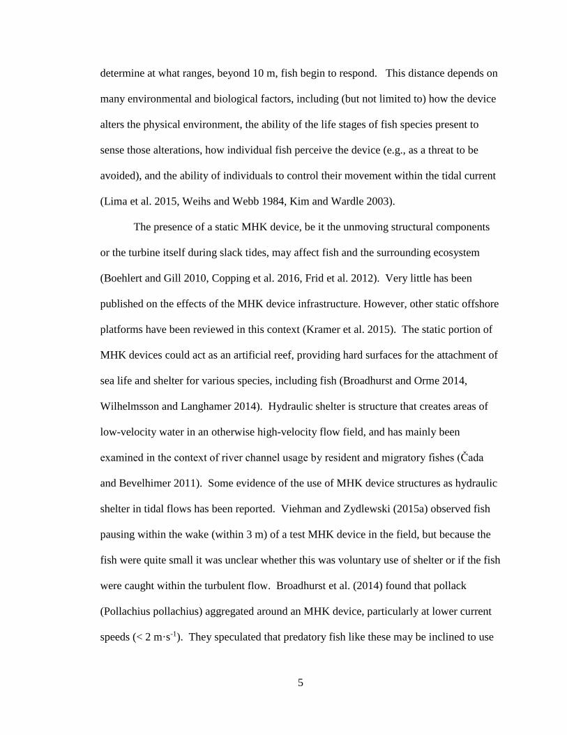
fish (i.e., the angular measurements along the major and minor axes of the beam). Many

tracks that were detected in the area of the turbine had accurate range measurements and

minor-axis angle estimates (position in the beam’s horizontal cross-section), but highly

14

variable major-axis angle measurements (position in the beam’s vertical cross-section;

Fig 1.5a). For this reason, the following analyses were carried out in 2 dimensions,

focusing only on fish heading (movement trajectory in the horizontal plane, relative to

north) and ignoring fish inclination (movement trajectory in the vertical plane, relative to

horizontal).

Even after limiting analyses to the horizontal plane, some poor-quality tracks

needed to be identified and removed from the 2D dataset. Poor-quality tracks were

therefore those that were physically improbable. These were tracks with highly tortuous

paths (Fig 1.5c,d), which were unlikely to be accurate. given the speed of the current and

the short time each fish spent within the beam (95% of fish detected remained in the

beam for 3 seconds or less. In reality, fish were most likely traveling in a roughly

straight line across the sampled volume (Fig 1.5a,b), consistent with previous

observations at this site (Viehman and Zydlewski 2015a). To help separate good and bad

tracks, a line was fit to each track using the time and position of the track’s single targets.

Six parameters were then calculated (in the horizontal plane) for each track to classify it

as either good or bad: the R2 of the line fit, the ratio of the straight-line distance between

the start and end points and the distance covered by the path, the polarity of the track

segments, the average distance of the track’s single targets from the fitted line, and the

average and standard deviation of the angles between consecutive track segments. Four-

hundred tracks were manually scrutinized and categorized as either ‘good’ or ‘bad.’ Half

of these tracks were used to build a general additive model (GAM) to predict track

quality based on the six factors, and half were used to test the model’s accuracy. This

method was found to reduce the prevalence of poor-quality tracks to less than 10% of the

15

final dataset. The prevalence of poor-quality tracks was similar (12%) when the model

was fit using the other half of the manually-scrutinized tracks, indicating a consistent

model regardless of the track subset used for fitting. More poor-quality tracks were

present in the turbine zone due to the acoustic interference from the support frame and

the turbine. The numbers of fish reported in each zone are therefore unlikely to represent

the true proportion of fish that passed through each, but their direction of movement

direction can still be used to assess their responses to the turbine. After poor-quality

tracks were removed from the dataset, the fitted line of each remaining track was used to

define fish heading, i.e., the direction of the track with respect to north.

16

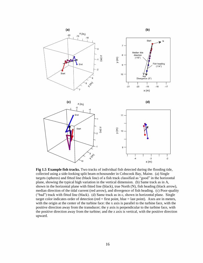
Fig 1.5 Example fish tracks. Two tracks of individual fish detected during the flooding tide,

collected using a side-looking split beam echosounder in Cobscook Bay, Maine. (a) Single

targets (spheres) and fitted line (black line) of a fish track classified as “good” in the horizontal

plane, showing the typical high variation in the vertical dimension. (b) Same track as in A,

shown in the horizontal plane with fitted line (black), true North (N), fish heading (black arrow),

median direction of the tidal current (red arrow), and divergence of fish heading. (c) Poor-quality

(“bad”) track with fitted line (black). (d) Same track as in c, shown in horizontal plane. Single

target color indicates order of detection (red = first point, blue = last point). Axes are in meters,

with the origin at the center of the turbine face: the x axis is parallel to the turbine face, with the

positive direction away from the transducer; the y axis is perpendicular to the turbine face, with

the positive direction away from the turbine; and the z axis is vertical, with the positive direction

upward.

17

1.3.2 Data analysis

The metric used to assess device effects on fish behavior was fish heading

divergence: the difference between each fish heading and the direction of the water

current. Generally speaking, at this site, fish move almost exclusively with the current

during the flowing tides and exhibit random ‘milling’ behavior at slack tides when

current speed is low (Viehman and Zydlewski 2015a). If fish normally travel with the

current, departure from the direction of the current may indicate a change in their regular

behavior, such as avoidance of the turbine or response to its wake.

We approximated water current direction as the median fish heading for each

individual tide. This approach was validated by comparing current speed data from an

ADCP briefly deployed on the sea floor at this site in March 2013 to concurrent fish

heading data collected using the same hydroacoustic setup from this study (Fig 1.6). Fish

heading in the March 2013 data followed a square-wave pattern (Fig 1.6a), with shifts

between high and low values corresponding to periods of slack tide as indicated by the

ADCP velocity data (Fig 1.6b). This pattern was very similar to current direction

measured and modeled at a nearby location by Xu et al. (2006). Additionally, fish

heading during the ebb and flood tides aligned very well with the average current

directions at this site (approximately 120° and 285°, respectively; ORPC personal

communication). Based on the March 2013 data, slack tides were defined as the 2-hour

periods which encompassed each shift in fish heading between ebb and flood directions.

For the current study, the times of these shifts were determined for the duration of the

dataset by fitting a sinusoidal model with tidal periodicities to the fish heading data, as

shown in Fig 1.6a and Chapter 3.

18

Fig 1.6 Fish heading and current velocity. Example from data collected at the TidGen® site in

March 2013. (a) Individual fish heading (gray points) shown with fitted tidal model (dashed line)

used to calculate times of slack tide (gray areas). (b) Current velocity collected concurrently by

a bottom-mounted ADCP at the same site.

Once slack tide periods were removed from the data, the median fish heading for

each individual ebb and flood tide was used as current direction during that time. If

fewer than 10 fish were present in a given tide, the median was not considered reliable,

and tracks from that tide were omitted from further analysis. Divergence was then

calculated for each fish track as the magnitude of the difference between its heading and

the corresponding estimated tidal current direction. This method helped avoid false

inflation of variation in fish heading due to shifts in flow over time.

Ebb and flood tides were analyzed separately because during flood tide, fish were

approaching the device, and during ebb tide, fish were departing from it. For each tidal

stage, a linear model (function lm in package stats in R) was used to test for effects of

four factors and their interactions on fish divergence from the current: static turbine state

19

(absent or present), sampling zone (beside or turbine), diel condition (day or night), and

fish size (TS). The continuous factor, TS, was centered at its mean, and to meet

assumptions of residual normality, the normal scores of divergence were used as the

response variable. The initial models included main factor effects as well as interaction

terms, and final models included only those terms that were found significant at the 5%

level (single terms that were part of significant interaction terms were also included).

1.4 Results

While the static turbine was present (2013), 4,104 good-quality fish tracks were

identified, and 4,696 while the turbine was absent (2014). More fish were tracked beside

the turbine than in the turbine zone during both the flood (Fig 1.7) and ebb (Fig 1.8) tides,

likely due to acoustic inference at turbine-zone ranges. More fish were detected during

the ebb tide than the flood tide. During the flood tide, we detected many more fish at

night than during the day (Fig 1.7), but there was not a large diel difference for the ebb

tide (Fig 1.8).

Over 90% of fish had TS ranging from -48 to -38 dB (Figs 1.7 and 1.8). This TS

range equates to fish lengths of approximately 4 to 11 cm using Love’s general lateral-

aspect equation, though this relationship varies greatly with fish species and orientation

(Love 1971). TS tended to be higher in the turbine zone than beside the turbine,

indicating larger fish, and this difference was more substantial when the turbine was

present. This apparent difference in size between zones was likely due to acoustic

interference from the MHK device (particularly the turbine), which made weaker acoustic

targets more difficult to track at the further range, where the turbine was located. TS also

appeared higher during the ebb tide than the flood tide, but this may have been due to

20

slightly different orientation of the fish with respect to the acoustic beam during different

tide phases than to actual size differences. The ebb tide current, and presumably the fish

moving with it, was more perpendicular to the acoustic beam’s central axis than the flood

tide current (Fig 1.3b), increasing the TS of fish detected at ebb tide relative to those

detected during flood-tide, which would travel at a more oblique angle (Boswell et al.

2009).

Fig 1.7 Target strength of fish detected during the flood tide. Fish moving with the current

would be approaching the MHK device. Shown is the distribution of target strength (TS) of fish

beside the turbine (white boxes) and in the turbine zone (grey boxes) during the day and night, (a)

when the turbine was absent, 2014; (b) when the turbine was present and static, 2013. Horizontal

line is the median, boxes span interquartile range, whiskers span 5th to 95th percentile, and points

indicate minima and maxima. Numbers are sample size of each group.

21

Fig 1.8 Target strength of fish detected during the ebb tide. Fish moving with the current

would be departing from the MHK device. Shown is the distribution of target strength (TS) of

fish beside the turbine (white boxes) and in the turbine zone (grey boxes) during the day and

night, (a) when the turbine was absent, 2014; (b) when the turbine was present and static, 2013.

Horizontal line is the median, boxes span interquartile range, whiskers span 5th to 95th percentile,

and points indicate minima and maxima. Numbers are sample size of each group.

Fish divergence from the current direction suggested that fish swam in the

direction of the current when the tide was flowing (Figs 1.9 and 1.10). Ninety-five

percent of all fish trajectories diverged from the current direction by 15° or less. Median

fish heading (e.g., estimated tidal current direction) ranged from 115° to 128° during ebb

tide and from 279° to 290° during the flood tide. Against-current movement was only

visually obvious in the turbine zone at night, when the static turbine was present (Fig

1.9b, lower right panel): approximately 4% of fish diverted more than 100° from the

median direction, whereas no more than ~0.3% did so in any of the other sets of

conditions. During this time, the polarity of the fish headings was 0.91, as opposed to

0.99 for all others (polarity of 0 would indicate completely random headings, and 1

would indicate completely uniform).

22

Fig 1.9 Fish heading and divergence during the flood tide. Fish moving with the current

would be approaching the MHK device. Histograms are heading ivergence from current

direction, and inset rose diagrams are fish heading relative to North. (a) When the turbine was

absent, 2014; (b) when the turbine was present and static, 2013. White and black bars correspond

to the beside-turbine zone and turbine zone, respectively. Gray background indicates night. The

number of fish (n) and the polarity of their headings (P) are shown for each group.

Fig 1.10 Fish heading and divergence during the ebb tide Fish moving with the current

would be departing from the MHK device. Histograms are heading ivergence from current

direction, and inset rose diagrams are fish heading relative to North. (a) When the turbine was

absent, 2014; (b) when the turbine was present and static, 2013. White and gray bars correspond

to the beside-turbine zone and turbine zone, respectively. Gray background indicates night. The

number of fish (n) and the polarity of their headings (P) are shown for each group.

23

Linear models fit to flood and ebb tide data were both statistically significant

(model p-values < 0.05), suggesting a relationship between the dependent variable (fish

divergence) and independent variables (turbine state, zone, diel stage, and TS). The

model fits were low, accounting for only 2.0% and 0.6% of the variation in fish

divergence for flood and ebb tides, respectively. The model therefore had little predictive

power. However, it did indicate that several factors affected fish behavior.

During the flood tide, when fish would have been approaching the MHK device,

turbine state and sampling zone had statistically significant main effects on fish

divergence at the 5% level (Table 1.3). There were also interaction effects involving

turbine state, sampling zone, and diel stage. Given these interaction effects, the fitted

values of the model for each combination of factors can best illustrate the relative

differences in divergence (Fig 1.11). These modeled values indicated that when the

turbine was absent, divergence was greater beside the turbine than in the turbine zone

during the day, but at night, there was no zone effect (Fig 1.11a). When the static turbine

was present, divergence was greater in the turbine zone than beside the turbine during

both day and night (Fig 1.11b). Divergence was higher at night for both sampling zones,

but the difference between zones was greater during the day.

24

Table 1.3 Linear model of fish heading divergence. Divergence is the difference between fish

heading and median direction. Shown are model results from fish detected during the flood tide

(when fish would have been approaching the MHK device).

Model term Coefficient

estimate

Standard

error

P-value

Intercept 0.208 0.058 <0.001

Turbine state (static) -0.554 0.090 <0.001

Zone (turbine) -0.348 0.104 0.001

Diel stage (night) -0.110 0.066 0.095

Turbine state (static):zone (turbine) 0.855 0.194 <0.001

Turbine state (static):diel stage (night) 0.363 0.098 <0.001

Zone (turbine):diel stage (night) 0.349 0.119 0.003

Turbine state (static):zone (turbine):diel stage (night) -0.475 0.223 0.033

Adjusted R2 0.019

Model p-value <0.001

Fig 1.11 Normal scores of divergence estimated by the linear model. Graphical

representation of the model summarized in Table 1.3, showing main and interaction effects of

significant factors: turbine state (static turbine absent or present), diel stage (day or night), and

sampling zone (beside or turbine). (a) Static turbine absent; (b) static turbine present. White and

gray points correspond to the beside-turbine zone and turbine zone, respectively. Gray areas

indicate night.

During the ebb tide, when fish would have been departing from the MHK device,

the only significant factor affecting divergence was TS (coefficient estimate: 0.038;

standard error: 0.012; p-value: 0.001). This indicated that larger fish showed greater

25

variation in movement with respect to the current than smaller fish, but divergence was

not influenced by turbine state, diel stage, or sampling zone.

1.5 Discussion

Fish approaching the MHK device responded to the static turbine at the distances

observed. The fish sampled were mainly small, likely on the order of a few cm in length,

and they generally traveled in the same direction as the tidal current. However, those

directly upstream of the static turbine showed more variable movement with respect to

the current than those that were to the side. This difference occurred when the static

turbine was present but was not apparent when the turbine was absent, and suggests

turbine avoidance. Previous studies of fish evasion of operating MHK devices have

sampled the first few meters from the turbine and observed evasion (Hammar et al. 2013,

Viehman and Zydlewski 2015a). As we observed a volume spanning 7-14 m from the

face of the static TidGen® turbine, our results suggest the range of MHK device effects

on fish behavior extends at least 18 m upstream, and perhaps farther for an operating

device. Shen et al. (2016) carried out transects over an MHK device similar to the

TidGen® with a rotating, but not generating, turbine, and they found evidence that fish

were moving out of the path of the device as far as 140 m upstream.

Reactions to the static turbine that we observed were generally confined to small-

scale adjustments in trajectory, as most fish (95% of tracks) diverged 15° or less from the

current direction. Evasion maneuvers have been observed to range from small-scale

adjustment to complete reversal of movement (Hammar et al. 2013, Viehman and

Zydlewski 2015a), but these studies occurred within a few m of the devices and involved

rotating turbines. At the distances from the turbine which we sampled here, slight

26

deflection from the strong current is likely an effective and energy-efficient method of

downstream obstacle avoidance. For the small fish that we sampled, it may also be the

only possible maneuver, as fish swimming power is directly related to length (Beamish

1978). Fish of Cobscook Bay are generally small, and consist mainly of juveniles of

multiple species (Vieser 2014, Zydlewski et al. 2016). During this study, a large portion

of fish sampled were likely larval or recently-metamorphosed juvenile Atlantic herring

(Vieser 2014, Zydlewski et al. 2016), which would be weak swimmers relative to the

tidal current. In their transects over a similar ORPC device, in August 2014, Shen et al.

(2016) observed slightly larger fish, which were likely a mix of juvenile Atlantic herring

(~20 cm) and adult Atlantic mackerel (~30 cm; Vieser 2014, Zydlewski et al. 2016).

Those fish would be stronger swimmers than the ones observed here in Apr-Jun 2012

and 2013, and they, too, moved almost exclusively with the current. As their numbers

decreased beginning 140 m upstream, and vertical distribution did not change, they too

were likely using small movements to avoid the downstream obstacle.

At multiple meters upstream of an MHK device, small movements in relation to

the current may be the chosen method of avoidance for both the small (< 10 cm) and

large (10-30 cm) fish. Within a few meters of the turbine, size may be of greater

importance to evasive behavior. In the first 3 m upstream of a rotating MHK turbine,

Viehman and Zydlewski (2015a) found that small fish (10 cm and under) tended to enter

the turbine if it was in their path, with at most 2% actively evading by swimming up,

down, or against the current. Larger fish (most of which were still less than 20 cm) had a

greater likelihood of evading the turbine (up to 11%), likely due to greater

maneuverability in the fast currents. Studies of fish responses to trawls have also found

27

close-range evasion to be stronger in larger fish (e.g., Rakowitz et al. 2012 and Sajdlová

et al. 2015). Fish size, and therefore species and life stage, is therefore an important

factor when considering if and how fish avoid MHK devices.

Avoidance of an MHK device also depends on whether fish can detect the device,

and at what range this occurs. Fish have a variety of sensory systems to alert them to

approaching objects, including visual and auditory senses and the lateral line system,

which is sensitive to the local flow field and may play a role in detecting distant, low-

frequency sounds (Popper and Schilt 2008, Bleckmann and Zelick 2009, Evans 1993).

As we saw evidence of avoidance during both day and night, fish were likely detecting

and responding to visual cues and non-visual cues (e.g. acoustic and hydrodynamic) from

the device. The turbine had a larger effect on fish divergence from the current during the

day than at night, indicating that sight played an important role in eliciting avoidance

behavior. This agrees with the close-range studies by Viehman and Zydlewski (2015a)

and Rakowitz et al. (2012), which found the probability of turbine and trawl evasion,

respectively, to be higher during the day than at night. However, at night we also

observed a small portion of fish (~4%) in the turbine zone that moved against the current,

which was not seen during the day or beside the turbine. It is possible that in the absence

of vision, the acoustic and hydrodynamic cues of the static device evoked stronger and

less uniform reactions to its presence. This would be in agreement with the less-directed

responses of herring to obstacles in the dark (Blaxter and Batty 1985) and of various fish

species to approaching trawls at night (Rakowitz et al. 2012).

We cannot rule out that the behavioral difference which we observed at night

could be related to different species or life stages of fish being sampled at that time.

28

During the flood tide, many more fish were detected at night than during the day, which

could have been the result of the activity of nocturnal species within the water column

(Reebs 2002, Vieser 2014), or of schools spreading out at night and the individuals from

the schools becoming trackable (Pitcher 2001). The result of either would be sampling a

different community of fish at night than during the day, and therefore comparing the

responses of fish with different sensory and locomotory abilities. TS during day and

night indicated that fish size did not change dramatically, but different species may

respond to the same cues in different ways. Species-dependent responses have been

observed for other MHK devices. Amaral et al. (2015) and Castro-Santos and Haro

(2015) found fish responses to turbines in laboratory flumes to be species-dependent,

with turbine responses related to each species’ swimming behavior (e.g., active rheotaxis

or passive drifting) and direction of travel (upstream- or down-stream migrating).

Hammar et al. (2013) found the same in the field, where they observed certain species

(mainly predatory fish) to be approach MHK turbines more than others, hypothesizing

that they were ‘bolder’ individuals. The species of fish present at a tidal power site and

how species composition changes over time must therefore be considered when

predicting or interpreting their responses to MHK devices, as the type of response will

largely determine the risk of entrainment, injury, and mortality.

In this study, we examined fish movement in the horizontal plane, but it is also

possible that fish responses to the MHK device were taking place in the vertical plane

(i.e., swimming upward or downward to avoid the upcoming turbine). Diving is

commonly observed as the primary reaction of fish to disturbances such as passing

vessels and approaching trawls (Ona et al. 2007, Sajdlová et al. 2015), often seen before

29

lateral movements and at great ranges (450 m, Handegard and Tjøstheim 2005; 75-275

m, Handegard et al. 2003). Additionally, Bevelhimer et al. (2015) found evidence of

downward fish movement 0-15 m from an HK device deployed in the East River, NY.

As such, we cannot rule out vertical avoidance of the TidGen® device at the ranges we

observed. Two other studies carried out at the same site as the present work provided

conflicting evidence of vertical movements in response to MHK devices. In their

transects over the MHK device, Shen et al. (2016) did not observe vertical fish

movements related to the device. On the other hand, Staines et al. (2015) found some

differences in the vertical distributions of fish near the TidGen® (~50 m away) before and

after its installation that may have been related to device presence. The different vertical

distributions may have resulted from vertical movements by fish, but this movement

could not be inferred from the distribution data used when observing these differences.

The acoustic data contamination which prevented us from assessing vertical

movement is a common issue in hydroacoustics, particularly when collecting data near

solid boundaries such as an MHK device, the seafloor, and the sea surface. Possible

methods of addressing this issue include using a narrower beam, (which could reduce

surface and bottom interference), moving the beam farther from the device (though this

could reduce the likelihood of observing fish responses), or using multibeam sonars

(Williamson et al. 2015, Melvin and Cochrane 2014). Additional improvements could

be made to the data processing techniques used here. Automated processing is necessary

for such large datasets, which are too time-consuming to process manually. The

processing method used here was effective at removing many types of noise from the

data, but it was also conservative and likely omitted many useable fish tracks from

30

analyses. Improvements to acoustic data processing techniques, such as incorporating

visual signal processing, could help reduce unnecessary data omission. Changing levels

of noise in different parts of the sampled volume resulted in unequal detection

probabilities over time and in different parts of the acoustic beam, making it impossible

to use fish numbers as indicators of turbine effects (e.g., beside vs. turbine zones, or

present vs. absent). However, overall, the diel and tidal differences in fish numbers that

we observed were consistent with a more detailed assessment of temporal patterns of fish

passage rate at this site (Chapter 3) and likely reflected natural patterns as opposed to

device effects.

Unlike the flooding tide, we saw no effects of MHK turbine presence on fish

movement during the ebbing tide, when they would be departing from the device. The

wake of the device can extend over 100 m before flow velocity reaches 90% of its

undisturbed magnitude (Rao et al. 2016), but fish apparently were not responding to it in

a way which we could detect. The only statistically observed effect on fish movement

downstream of the device was of fish TS, which suggested that larger fish were diverging

farther from the current direction than smaller ones, regardless of turbine presence.

Viehman and Zydlewski (2015a) reported that fish were almost always milling in the

wake of the test turbine they examined, though that viewing window extended only 3 m

downstream of the device. Those fish may have been sheltering from the fast currents in

the low-velocity area just behind the turbine structure (Čada and Bevelhimer 2011), or

were potentially disoriented by turbine passage or the sudden change in flow conditions.

Regardless of the cause of the turbine-wake milling behavior, if it was occurring near the

31

static TidGen® in the present study, it did not extend beyond 7 m downstream of the

turbine.

To predict and interpret fish responses to MHK devices, we need a better

understanding of the physical signature of the static and dynamic devices. To date,

detailed measurements of the visibility, noise generation, and hydrodynamic signatures of

MHK devices are sparse and spread over a wide range of designs and deployment

configurations (Copping et al. 2014). Measuring these physical conditions around MHK

devices in strong tidal currents poses its own set of challenges (e.g., Martin and Vallarta

2012) but in many cases is more easily accomplished than observing fish behavior at all

the possible spatial and temporal scales of interaction. The distance at which fish detect

and respond to MHK devices will depend on the fish present and site characteristics, as

detection thresholds of fish sensory systems (e.g. vision, hearing, and the lateral line)

vary with species and life stage and their sensitivity is modified by environmental

conditions (Kim and Wardle 2003, Bleckmann and Zelick 2009, Blaxter 1986).

Knowledge of the physical “footprint” of MHK devices, combined with knowledge of the

sensory capabilities of the fish that may encounter them, would aid in planning studies of

fish behavior by identifying where fish are most likely to detect and respond to the

device, and would afterward inform interpretation of study results. Our understanding of

fish sensory abilities is limited, and more information on a wider range of marine species

would be necessary for this approach.

To develop a better understanding of how fish interact with MHK devices, we

should aim to collect concurrent information on the physical signatures of devices and the

behaviors of fish encountering them. Williamson et al. (2015) have taken a step in this

32

direction by developing a bottom-mounted monitoring platform that includes multibeam

and split beam echosounders, a flow meter, and a fluorometer, with the possibility for

adding other equipment. Collecting data with these instruments simultaneously may

allow animal behavior to be linked to local physical conditions affected by MHK devices;

for example, fish movement with respect to the turbulence generated downstream.

Studies using integrated approaches such as this will help build a more complete

understanding of how and why MHK devices affect fishes and other marine organisms.

The results of this study and others indicate the effects of an MHK device on fish

will vary with the species and life stages that are present at the same location. At a tidal

energy site, the composition of the fish community is likely to change on a variety of

spatial and temporal scales (Chapter 3, Vieser 2014), and the effects of proposed MHK

devices must be assessed with these changes in mind. As more individual devices are

deployed and monitored, preferably with integrated biological and physical monitoring

systems, we can begin to expand predictions of effects from individual animals and

devices to population-level effects and device arrays. This information can inform the

design and location of MHK device arrays as we seek to responsibly develop this

renewable energy source.

33

CHAPTER 2

POTENTIAL OF SINGLE BEAM ECHOSOUNDERS FOR

ASSESSING FISH AT TIDAL ENERGY SITES

2.1 Abstract

Hydroacoustics is a valuable tool for assessing fish presence, relative abundance,

and size. Scientific-grade split beam echosounders provide the most information on

individual fish but can be prohibitively expensive for start-up companies exploring

potential tidal energy development sites where fish interactions with their devices must

be monitored. Commercial-grade, single beam echosounders are significantly less

expensive than split beam echosounders but provide less information as they cannot

correct the echo strengths of individual fish (TS) to account for the effect of the beam

pattern, complicating size and species estimates. Statistical methods, i.e. deconvolution,

exist to correct TS distributions for the beam pattern effect and could expand the utility of

single beam systems for tidal energy site assessment. We applied deconvolution

techniques to single beam data from a study at a tidal energy site in Cobscook Bay,

Maine. Fish were detected in hydroacoustic data collected concurrently with a wide-

angle (31o) single beam echosounder and a narrow-angle (7o) split beam echosounder in

two 24-hr surveys in August 2012 and March 2013. For each survey, the distribution of

TS data from the split beam echosounder (compensated for beam pattern) was the

reference distribution. This was compared to two deconvolved “single beam” TS

distributions: one from the wide-angle single beam TS data, and one from the narrow-

angle split beam TS data uncompensated for beam pattern, which represented data from a

narrow-angle single beam. We found that deconvolution was not effective in March,

34

when few fish were present (141 and 80 detected fish, for single and split beam,

respectively), but was more effective in August, when more fish were sampled (501 and

377 fish). In August, the deconvolved TS distribution from the wide-angle single beam

did not resemble the reference TS distribution, likely due to a large proportion of

multiple-target echoes being misclassified as single targets. On the other hand, the

deconvolved distribution of the uncompensated split beam TS did resemble the reference

distribution, indicating narrow-angle single beam echosounders may provide good

estimates of fish TS. However, the smaller volume sampled by a narrow beam could also

hamper investigations of shallower, faster sites, or when fewer fish are present. If TS

information is not needed, wide-angle single beam echosounders may be sufficient for

tidal energy site monitoring as they can still provide a relative index of fish density.

Depending on the required information, the use of either single beam system could

greatly reduce costs of environmental assessment for tidal energy developers.

2.2 Introduction

Tidal energy is a new form of renewable energy that uses large, underwater

turbines to convert the kinetic energy of tidally-generated currents to electricity. Few of

these marine hydrokinetic (MHK) devices have been deployed worldwide, so their

environmental effects remain largely unknown. In most permitting procedures,

developers are required to carry out assessments of the environmental effects of their

devices (Jansujwicz and Johnson 2015, Henkel et al. 2013).

Fish are a key part of the marine ecosystem that may be affected by MHK devices

(Copping et al. 2016). Hydroacoustics is one of the best tools for collecting data on fish

at sites targeted for tidal power development (Viehman et al. 2015). Hydroacoustics is a

35

type of sonar specialized for detecting fish in the water column, and allows large volumes

of water to be sampled simultaneously with high temporal and spatial resolution

(Simmonds and MacLennan 2005). Additionally, it is well-suited to collecting data in

areas with fast currents and complex bottom bathymetry, where physical sampling

methods, such as trawling, would not be safe or effective (Viehman et al. 2015, Vieser

2014, Williamson et al. 2015).

Echosounding systems range in complexity and accuracy. Scientific-grade split-

beam echosounders allow fish to be tracked within their beam in three dimensions, which

is useful in assessing their responses to stimuli (Chapter 1; McKinstry et al. 2005). The

ability to pinpoint a fish’s location within the acoustic beam also allows their returning

echo strengths to be accurately corrected for the effect of beam pattern (Simmonds and

MacLennan 2005). An acoustic beam ensonifies an approximately conical volume

extending away from the transducer, and is strongest along its central axis (“on-axis”)

and weakens toward the edges (“off-axis”). The acoustic reflection, or target strength

(TS), of a fish on-axis will be recorded at its true strength, but those at greater angles

relative to the central beam axis will be recorded as weaker acoustic targets than they

actually are. If the beam pattern is known, the location of each fish relative to the beam’s

central axis can be used to correct, or compensate, the TS of each individual. The

resulting compensated TS can then be used to roughly estimate fish size and therefore, to

some extent, species (Simmonds and MacLennan 2005). However, the cost of these

systems, upwards of $50,000 US, is often unrealistically high for small-scale tidal

developers, particularly if a site has not yet proven to be worth developing.

36

A less expensive alternative is the single beam echosounder, on the order of

$10,000 US, which is the precursor to dual- and split-beam systems. These echosounders

can be used to determine the range of an acoustic target but cannot locate it within the

beam’s cross-section. They therefore cannot be used to track fish in 3D or correct the

returning echoes for beam pattern effects, resulting in less accurate TS and size estimates.

Commercial-grade single beam echosounders are the least expensive, but require careful

calibration by the user since factory calibrations are not as thorough as for scientific-

grade equipment. Their lower cost makes them much more attainable for tidal power

developers that are beginning to explore potential sites. However, the information that

can be directly provided by these systems (e.g., TS) is limited without the application of

more involved statistical techniques.

We used a commercial-grade single beam echosounder to conduct the initial

assessments at targeted tidal power sites in Western Passage and Cobscook Bay, Maine

(Viehman et al. 2015). Ocean Renewable Power Company (ORPC) was interested in

installing its MHK device, the TidGen® power system (Fig 2.1), in one or both of these

channels. Industry regulators were interested in the vertical distribution of fish in the

water column, and if they were likely to encounter the fixed-depth tidal power turbine or

not. Additionally, regulators wanted a baseline index of fish abundance for comparison

to future data that would be collected if development continued.

37

Fig 2.1 Ocean Renewable Power Company’s TidGen® Power System. Turbine image

provided by ORPC.

A single beam echosounder was sufficient to meet these research goals, as volume

backscatter (SV), a summation of the acoustic energy reflected within the acoustic beam,

serves as a relative index of fish density that does not require correction for beam pattern

effects. We chose to use a wide-angle (31°), dual-frequency (38 and 200 kHz)

commercial-grade transducer (the Simrad 38/200 Combi W), which we mounted over the

side of a vessel that was moored at each site for 24 hrs. The wide beam allowed us to

sample fish more effectively in the fast currents than a narrow beam, particularly in the

upper part of the water column where the beam was narrowest. The dual frequencies

were useful in separating fish from other sound scatterers, such as zooplankton (Staines et

al., submitted), and we found that fish tended to be densest near the surface or seafloor

(depending on the time of year), outside of the depth of the turbine (Viehman et al. 2015).

Based on the baseline results from that study and other environmental studies carried out

by ORPC and its partners, a pilot license permit was issued to further develop the

Cobscook Bay site (FERC 2012) At that point, more detailed information about fish

became important to regulators, including their sizes, species, and their behavior in

response to the MHK device.

38

The necessity for more detailed information on individual fish justified the use of

a scientific-grade split beam echosounder. This was especially needed to study the

movements of individual fish near the MHK device (Chapter 1). However, it is possible

that a single beam echosounder could be sufficient for obtaining information on the TS of

the fish sampled. Before the more complex dual and split beam echosounders were

developed, data from single beam echosounders were corrected for the effect of beam

pattern using statistical techniques, including deconvolution (Clay 1983). While not as

accurate as distributions obtained using individually-compensated fish TS from split

beam systems, some comparisons have found that narrow-angle (7°) single beam TS

distributions corrected in this manner agree well with dual- and split-beam data (Clay and

Castonguay 1996, Rudstam et al. 1999).

Only data from single fish should be used in deconvolution (Clay 1983, Stanton

and Clay 1986), so deconvolution in fisheries hydroacoustics has typically been confined

to narrower acoustic beams. This is because the volume sampled per range increment is

smaller for narrower beams, which lowers the likelihood that multiple fish would pass

through the same sampled volume at once and be falsely recorded as a single fish

(Simmonds and MacLennan 2005). In shallower areas, particularly with fast currents, it

can be beneficial to sample with a wider beam, as fish passing by quickly may be under-

sampled at closer ranges if the beam is very narrow. We wanted to determine if the

acoustic returns from a wide-angle single beam echosounder could be corrected to

account for the effect of its beam pattern via deconvolution techniques. If so, more

information could be provided by initial site assessments using the wide-angle single

beam echosounder, and we could improve the continuity between initial assessments

39

made with the single beam and later assessments carried out with the narrow-angle split

beam. If the method works, a single beam system could be sufficient for much of the

monitoring at tidal energy sites. This could greatly reduce costs for developers while still

providing detailed information for industry regulators.

To assess the utility of the deconvolution method for this application, we used

data collected concurrently with our narrow-angle scientific-grade split beam and wide-

angle commercial-grade single beam echosounders at the tidal energy site in Cobscook

Bay, Maine. The deconvolution methods of Clay (1983) were applied to the single beam

backscatter data, as well as to the uncompensated split beam backscatter, which is

effectively data from a narrow-angle single beam. These results were compared to

compensated split beam backscatter from the split beam echosounder, which was

assumed to represent reality. In this way, we assessed the utility of wide- and narrow-

angle single beam echosounders in tidal power site assessment.

2.3 Methods

Data were collected simultaneously with single and split beam echosounders,

using survey protocols at a tidal energy site in Cobscook Bay, Maine (Viehman et al.

2015). The split beam was a Simrad EK60 echosounder with a 7° circular-beam

transducer, and the single beam was the same as that used in initial site assessments: a

Simrad ES60 echosounder with a 38/200 Combi W 31° single beam transducer. The

transducers were mounted over the side of a vessel, which was moored near the TidGen®

(Fig 2.2) for 24 hr per survey, as in Viehman et al. (2015). Both transducers had a ping

rate of 2 s-1 (sampled the water column twice per second). The split beam operated with a

pulse duration of 0.064 ms (vertical resolution of approximately 5 cm) and power of 120

40

W, and the single beam used a pulse duration of 0.512 ms (vertical resolution of

approximately 38 cm) and power of 225 W. The single beam system used a longer pulse

duration than the split beam in order to match previously collected data (Viehman et al.

2015), in which a long pulse duration was required to reduce interference between the

single beam and DIDSON acoustic camera that was operating simultaneously.

Fig 2.2 Study area. Location of TidGen® and down-looking 24-hr hydroacoustic surveys shown

in right panel.

Two 24-h surveys were used for these comparisons: one from August 2012 and

one from March 2013. These two surveys were chosen based on the number of fish

present: fish abundance peaks in Cobscook Bay in the late summer into fall, and reaches

a minimum in the winter and early spring (Viehman et al. 2015, Chapter 3). Generally,

deconvolution requires many fish detections in order to work (Simmonds and

MacLennan 2005), so it was necessary to determine if the method could be useful for

data from a typical 24-hr survey when fish were scarcest. These two datasets are typical

of the BACI surveys that we have carried out at this site, and therefore are representative

of the data that would be available for this method in the future.

41

The single beam echosounder collected data with 38 kHz and 200 kHz

frequencies. Only the 200 kHz data were used in the following analyses. Future

reference to the single beam data therefore only refers to the 200 kHz frequency.

2.3.1 Echosounder calibration

Both echosounders were calibrated using a 13.7 mm copper calibration sphere,

with nominal TS of -45 dB.

The EK60 split beam echosounder was calibrated using the Simrad Lobes

program. This program records the position and uncompensated TS of the sphere as it is

swung through the beam multiple times, until many readings have been obtained from all

parts of the beam cross-section. The program then returns minor and major axis beam

angles, gain, and Sa corrections (Table 2.1). These calibrations were done in situ during

surveys.

The ES60 single beam echosounder cannot record the 3D location of targets

within the beam, so calibration was carried out differently. In situ on-axis calibrations

were performed at slack tide during surveys but were meant only to detect any significant

equipment malfunction, as the water was never still and the sphere could not be

accurately positioned. Full ES60 calibrations took place on a frozen-over lake in the

winters of 2011, 2013, and 2014. For these calibrations, the transducer was lowered

below the ice through one hole, leveled, and stabilized. The calibration sphere was then

lowered to known depths through a series of holes at known distances from the

transducer, including at the central beam axis. As the water was very still, we were able

to position the sphere within the beam at a variety of known off-axis angles and obtain

42

the corresponding uncompensated sphere TS. With these measurements, we calculated

the beam pattern parameters needed for deconvolution, as well as gain and Sa corrections.

2.3.2 Data processing

Hydroacoustic data were processed in Echoview® software (6.1, Myriax, Hobart,

Australia). The calibration parameters obtained from the frozen lake calibrations (single

beam) and in situ calibrations (split beam) were applied to the data collected in Cobscook

Bay. A -60 dB threshold was then used for single beam TS data, which would ensure

fish of -54 dB and higher were detected within the half-power beam angle and eliminate

most backscatter from small non-fish targets (e.g., zooplankton; Simmonds and

MacLennan 2005). A -54 dB threshold was applied to the compensated split beam TS

data (TS that had already been corrected for beam pattern). Additionally, after being

exported from Echoview®, split beam fish tracks with minimum uncompensated TS

below -60 dB were removed from the split beam dataset. These two thresholding steps

helped ensure that the fish included in the split beam data were similar to those included

in the single beam data, making the datasets more directly comparable.

The only noise removal necessary was to omit any data that were contaminated by

entrained air, and to remove any data where echoes from individual fish were likely to

overlap. To reduce the number of multiple targets falsely identified as individuals, single

target tracking parameters were chosen to accept the least distorted echoes (Table 2.1).

Fish tracks were additionally visually inspected to remove any that clearly came from

more than one fish (e.g., crossed tracks).

43

Table 2.1 Single target detection parameters. Parameters were used in Echoview® software to

detect and track individual fish.


Single target

detection: single

beam method 2

TS threshold -60 dB


Min. normalized pulse length 0.20

Max. normalized pulse length 2.00

Single target

detection: split

beam method 2

TS threshold -54 dB





Max. beam compensation 10.00 dB

Max. standard deviation of:



Pulse length at 6 dB (normalized) 0.70 to 1.30



Fish were tracked using Echoview®’s 2D tracking algorithm for single beam data

and the 4D tracking algorithm for split beam data (Table 2.2). Track TS was then

exported for further analysis in R. TS data exported for the single beam were

uncompensated for beam pattern, and TS data exported for the split beam included both

compensated and uncompensated values.

44

Table 2.2 Single beam (2D) and split beam (4D) fish track detection parameters. Parameters were used in Echoview® software to detect and track individual fish.


Fish tracking: 2D Data 2D

Alpha (range) 0.7

Beta (range) 0.5

Exclusion distance (range) 0.4 m

Missed ping expansion (range) 0 %

Weights:

Range 40

TS 0

Ping gap 0

Min. number of single targets in a track 5

Min. number of pings in a track 5 pings

Max. gap between single targets 3 pings




Exclusion distance

(major, minor, range)

4, 4, 0.4 m

Missed ping expansion

(major, minor, range)

0, 0, 0 %

Weights:

Major axis 30

Minor axis 30

Range 40

TS 0

Ping gap 0




2.3.3 Deconvolution

Deconvolution is a signal processing technique which reverses the effects of

convolution, which is when a signal is modified by another signal prior to measurement.

In the case of data from a single beam echosounder, the true probability density function

(PDF) of the backscatter of fish randomly distributed across the beam, wF(e), has been

convolved with that of the beam pattern, wT(b), to result in the measured backscatter

45

PDF, wE(e) (see calculation of the PDFs, below). Using the notation of Clay (1983), the

convolution is

𝑤𝐸(𝑒) = 𝑤𝑇(𝑏) ∗ 𝑤𝐹(𝑒) [1]

where * indicates convolution, the character “e” represents backscattering strength

(instead of the conventional σbs, for consistency with Clay 1983 and Stanton and Clay

1986), and b is beam intensity. Convolution becomes simple multiplication if the signals

are represented in the frequency domain:

𝑊𝐸(𝛼) = 𝑊𝑇(𝛼)𝑊𝐹(𝛼) [2]

where WE(α), WT(α), and WF(α) are the Fourier transforms of the PDFs. Deconvolution

consists of solving equation [2] for WF(α) and using the inverse Fourier transform to

recover wF(e).

The numerical deconvolution approach presented in Clay (1983) was used to

recover wF(e) from wE(e), using the known beam pattern PDF wT(b). This method

applied z-transforms to convert the two known PDFs into polynomial expressions in the

frequency domain. Polynomial long division was then used to calculate wF(e) using

equation [2]. Matlab’s function deconv, adapted to work in R, was used for this purpose.

The result, wF(e), was the fish backscatter PDF that had been corrected for the effect of

the beam pattern. The PDF was translated to a number of fish per backscatter bin by

multiplying the PDF probabilities by the total number of fish detected, as the sum of all

probabilities in a PDF is 1. For ease of visualization and interpretation of results,

backscatter was converted to TS (with units of dB) using the relationship

𝑇𝑆 = 10 log10(𝑒) [3]

46

2.3.4 Beam pattern PDF

For both transducers, data from calibrations were used to calculate the dB dropoff

(dBdrop(θ)) at different off-axis angles (θ) within the beam:

𝑑𝐵𝑑𝑟𝑜𝑝(𝜃) = 𝑇𝑆𝑒𝑥𝑝−𝑇𝑆𝑚𝑒𝑎𝑠(𝜃)

2 [4]

where TSexp is the expected on-axis TS (in dB re 1 m2) of the standard sphere under the

given environmental conditions (salinity, temperature, and pressure;

http://swfscdata.nmfs.noaa.gov/AST/SphereTS), TSmeas(θ) is the measured TS of the

sphere at θ, and dBdrop(θ) is the dB dropoff at θ, in dB. The difference in TS is divided by

2 because the observed TS difference includes energy lost while sound traveled the

distance between the transducer and the sphere twice: first, to the sphere from the

transducer, then once reflected, to the transducer from the sphere. The beam pattern,

B(θ), was modeled as a function of θ using a second order polynomial

B(θ) = 0 + c1θ + c2θ2 [5]

where B(θ) is in dB, and c1 and c2 are constants. B(θ) was then converted to its linear

form

𝑏(𝜃) = 10𝐵(𝜃)/10 [6]

where b(θ) is the directivity of the transducer, ranging from 1 on the central axis and

decreasing toward 0 as θ increases. For a given distance from the transducer, b(θ) is the

ratio of the echo amplitudes of a target at off-axis angle θ and a target located on-axis.

The beam PDF is the function that describes the probability of a point randomly located

within the beam’s cross section having intensity b. To estimate the beam PDF function,

equations [5] and [6] were used to calculate b for 1000 generated points, randomly

distributed across the acoustic beam with beam pattern B(θ). These points were divided

47

into intensity bins of equal width in the log domain, and the proportion within each bin

was calculated to estimate the beam PDF. More fish were present in August 2012, which

allowed the use of smaller intensity bins than March 2013 (see below), so beam intensity

was divided into 20 equally spaced bins per decade (order of magnitude difference) for

deconvolution of August data, and into 10 bins per decade for March data. The PDF of

the beam pattern, wT(b), was then fit to the estimated probabilities, P(b), in the form:

wT(b) = A ∙ P(b)−B [7]

where A and B are constants. In this process, b was limited to the range 0.005 to 1. The

minimum value of 0.005, which corresponds to a dB dropoff of -23 dB, was chosen based

on recommendations in Clay (1983) and Stanton and Clay (1986) to avoid the first side-

lobe level.

2.3.5 Fish echo PDF

The mean backscattering strength (units of m2) of tracked fish was treated in the

manner outlined by Stanton and Clay (1986). Fish TS was first converted to

backscattering strength (e) using

𝑒 = 10𝑇𝑆

10 [8]

The next steps followed the process for the beam pattern PDF: fish backscatter

data were divided into backscattering bins of equal width in the logarithmic domain, with

20 steps per decade in August 2012 (in the TS scale, each bin was 0.5 dB wide) and 10

steps per decade in March 2013 (1.0 dB wide in the TS scale). The counts from these

backscatter bins were divided by their sum to attain the fish echo PDF, wE(e).

Deconvolution is sensitive to noise, so wE(e) was then smoothed with a method similar to

that described by Stanton and Clay 1986 (Fig 2.3). A smoothing window of length n was

48

chosen, and a third-order polynomial was fit to the first n/2 points on either side of each

point in the PDF. The modeled values within each intensity bin were then averaged to

achieve the values for the final smoothed PDF to be used in deconvolution.

Fig 2.3 Smoothing of the echo PDF of fish detected. Shown is the echo PDF of fish detected in

August 2012 by the wide-angle single beam echosounder. The vertical axis is the probability that

fish backscatter falls within each backscatter bin, with points located horizontally at the center of

their respective bins. Original PDF shown in black, modeled points from smoothing process

shown in gray, and final smoothed PDF (average of modeled points in each backscatter bin)

shown in red. TS is the logarithmic form of fish backscatter, and has units of decibels.

Smoothing window was 0.5 times the length of the PDF.

Deconvolution results were sensitive to the width of the smoothing window that

was used. Previous work has chosen smoothing parameters by visual inspection of the

results (Clay 1983), judging whether variation was real or noise. We also chose the best

smoothing window by eye, but in addition to evaluating the deconvolved fish TS

distributions, we inspected the effects of the smoothing window on deconvolved

calibration sphere TS (Fig 2.4). The longest windows (0.6 or more times the length of

the echo PDF) worked the best for the calibration sphere but appeared to over-smooth the

fish TS distributions, and the shortest windows (0.4 or less times the length of the echo

49

PDF) preserved variation in the fish TS distributions but introduced large noise spikes to

the calibration sphere TS distribution. The final smoothing window was a compromise

between the two extremes (window width of one half the length of the PDF; Fig 2.4b).

Fig 2.4 Results of deconvolution of sphere TS. Three different smoothing window lengths were

used: (a) 0.7, (b) 0.5, and (c) 0.3 times the length of the PDF.

2.3.6 Assessment of deconvolution accuracy

To test the performance of the deconvolution method, the compensated

backscatter from the split beam echosounder was used as a reference. Compensated

backscatter is backscatter that has been corrected for beam pattern for each individual

fish based on its location within the beam, and was assumed to be representative of

reality. Uncompensated backscatter from the split beam is equivalent to backscatter

from a single beam of equal dimensions, as it has not been corrected for beam pattern.

Uncompensated split beam data were deconvolved using the split beam pattern, and the

result was compared to the compensated data to assess the functionality of the method for

a narrow-angle single beam echosounder. The backscatter of fish detected with the wide-

angle single beam echosounder was deconvolved using the single beam pattern

(generated from the ice calibration data), and those results were also compared to

50

compensated backscatter from the split beam echosounder. Kolmogorov-Smirnov tests

with a significance level of 0.05 were used to verify visual comparisons.

2.4 Results

2.4.1 Transducer calibration

The scientific-grade split beam calibration matched the factory-provided

calibration data (Fig 2.5, Table 2.3). The commercial-grade single beam echosounder had

a slightly narrower beam than expected (Fig 2.5, Table 2.3). The greater uncertainty in

sphere position with the single beam echosounder is evidenced by the greater variation in

readings at each off-axis angle, compared to the split beam. Both transducers’ beam

patterns were well-represented by the second degree polynomial fit to the data in the TS

domain.

Fig 2.5 Results of echosounder calibrations. Beam pattern shown as (a) dB dropoff and (b)

intensity at a range of off-axis angles. Points are calibration data, the thick lines are models fit to

each echosounder’s calibration data, and the dashed lines are the factory-specified beam patterns

of each transducer.

51

Table 2.3 Single and split beam data calibration parameters. Split beam values were

obtained from in situ calibrations in August 2012 and March 2013. Single beam values were

based on winter calibrations carried out in 2011, 2013, and 2014.

Parameter Split beam

Single beam August 2012 March 2013

3 dB (half-power) beam angle 6.6° (major axis)

6.5° (minor axis)

6.5° (major axis)

6.6° (minor axis)

24.8°

Gain 25.7 dB 26.0 dB 8.5 dB

Sa correction -0.5 dB -0.6 dB - 0.3 dB l

2.4.2 Beam pattern PDF

The PDF of the beam for each echosounder (Fig 2.6) matched expectations,

indicating the probability of receiving a full-intensity (e.g., on-axis) echo was lower than

the probability of receiving weaker-intensity (e.g., off-axis) echoes. Targets within the

narrow-angle split beam are more likely to have higher intensities than those within the

wide-angle split beam, and less likely to have very low intensities, due to the shape of

each beam.

Fig 2.6 Beam pattern probability density function. wT(b) shown for the 200 kHz single and

split beam echosounders, with (a) logarithmic and (b) linear axes. Vertical line indicates

minimum intensity included in analyses (0.005). The beam intensity shown is squared, as sound

is affected by the beam pattern twice as it travels to and from a reflective object.

52

2.4.3 Fish echo PDF

More fish were detected in August than in March, as expected (Fig 2.7), and more

were detected by the wide-angle single beam than the narrow-angle split beam. In

August 2012, 501 fish were detected by the single beam, but the split beam detected only

377 fish. In March 2013, only 141 fish were detected by the single beam, and 80 by the

split beam. In both months, the distribution of uncompensated single beam backscatter

had greater contributions from stronger targets than the uncompensated split beam (Fig

2.7a). In March, the low sample sizes of the split and single beam datasets resulted in

highly variable, low-resolution TS distributions (Fig 2.7b).

Fig 2.7 Distribution of TS data from single beam and split beam echosounders. (a) August

2012 and (b) March 2013. Data were divided into 20 backscatter bins per decade in August, and

10 per decade in March. The number of fish in each sample (N) shown in upper right. Thick lines

indicate smoothed TS distributions (using a window size of 0.5 times the PDF length) which were

used in deconvolution.

2.4.4 Deconvolution

For the split beam echosounder data, in August 2012, deconvolved

uncompensated backscatter followed a similar distribution as the compensated

backscatter, with a main peak near -50 dB and a left skew (Figure 2.8a). However, the

53

deconvolved distribution also had a small secondary main peak near -54 dB which was

not present in the compensated data. Also, in its tail, the deconvolved distribution had

smaller peaks centered near -43 dB and -40 dB that were not evident in the compensated

distribution. All compared distributions were significantly different at the 5% level

(Kolmogorov-Smirnov p-value < 0.05).

In March 2013, the deconvolved split beam backscatter did not match the

compensated backscatter well (Fig 2.8b). Compensated backscatter indicated a main

peak near -49 dB, a secondary peak at -44 dB, and a small peak at -39 dB. The

deconvoluted backscatter showed peaks near -52 dB, -47 dB, and -44 dB.

Fig 2.8 Results of deconvolution of uncompensated backscatter from the split beam

echosounder. (a) August 2012 and (b) March 2013. Uncompensated (magenta), deconvolved

(blue), and compensated (green) TS distributions are shown. The number of fish in each sample

(N) shown in upper right. The thick magenta line shows the smoothed TS distribution (using

window length of 0.5 times the PDF length) that was used in deconvolution, and the thin magenta

line shows the unsmoothed TS distribution. Data were divided into 20 backscatter bins per

decade in August, and 10 per decade in March.

54

For the wide angle, commercial-grade single beam echosounder, in August 2012,

the deconvolved distribution was bimodal, with one peak centered below the peak of the

compensated split beam backscatter (-50 dB) and the other, larger peak at -44 (Fig 2.9a).

In March 2013, the deconvolved single beam backscatter distribution was trimodal, with

peaks at -49, -44.5, and -40 dB (Fig 2.9b). These peaks were close to those of the

compensated split beam backscatter, but had very different relative sizes, with most

echoes in the smallest and largest peaks, and relatively few in the center one.

Fig 2.9 Results of deconvolution of uncompensated backscatter from the single beam

echosounder. (a) August 2012 and (b) March 2013. Uncompensated (magenta) and deconvolved

(blue) single beam TS distributions are shown, as well as the compensated (green) split beam TS

distribution. The number of fish in each sample (N) shown in upper right. The thick magenta line

shows the smoothed TS distribution (using window length of 0.5 times the PDF length) that was

used in deconvolution, and the thin magenta line shows the unsmoothed TS distribution. Data

were divided into 20 backscatter bins per decade in August, and 10 per decade in March.

55

2.5 Discussion

Deconvolution did not adequately correct backscatter data from the wide-angle,

commercial-grade single beam echosounder. While the smaller peaks in the deconvolved

TS distributions aligned well with reality (the compensated split beam TS distribution), in

both surveys, there was a large peak at stronger TS that was not evident in the

compensated split beam data. This large peak was likely the result of multiple targets

being falsely interpreted as single targets. The single beam’s long pulse duration meant

that fish passing through the beam at the same time would need to be separated vertically

by at least 38 cm to be distinguished from each other. The wide angle increased the

likelihood that more than one fish would be present in the beam at similar depths at any

given time. Multiple fish interpreted as one target would have stronger TS than the

individual fish involved (Simmonds and MacLennan 2005). Deconvolution of data

comprised of a mix of single targets and single targets that were actually multiple targets

would result in the bimodal TS distribution that we observed, with one peak near the true

TS and the other at stronger TS. Without the reference provided by the split beam

echosounder, we would not have known that the peak at stronger TS was false, and may

have concluded that the fish community sampled had a bimodal length distribution.

Given this high uncertainty, it is likely best to limit the use of the wide-angle single beam

to relative density measurements (e.g., Viehman et al. 2015, Staines et al. 2015).

Some steps could be taken to improve the suitability of wide-angle single beam

data for deconvolution techniques. First, the pulse duration could be reduced, e.g. to

0.064 ms, like the split beam. Using a shorter pulse duration would decrease the volume

of each vertical sample, and therefore decrease the likelihood of detecting multiple fish

56

and classifying them as individuals. Second, single target detection parameters could be

stricter. The shape of the echo returned by many targets, as opposed to single targets, is

more distorted relative to the sound pulse output by the transducer (Simmonds and

MacLennan 2005). Accepting only the least distorted echoes would reduce the multiple

targets accepted as single targets. In the present study, further restricting single target

acceptance would have eliminated many of the tracked fish. As our sample sizes were

already quite low for deconvolution, using stricter single target detection parameters

would require collecting data for longer periods of time, particularly at times of the year

when fish are scarce. However, sampling for multiple days per survey could more than

offset any savings gained by using a single beam transducer, in which case it would be

best to use a split beam and acquire accurate TS information for individual fish.

While deconvolution may not be sufficient to correct data from a wide-angle

single beam for TS, it may provide useful information for a narrow-angle single beam

using a short pulse duration. Deconvolution of the uncompensated split beam backscatter

yielded a TS distribution that appeared very similar to that of the compensated data,

though shifted slightly toward weaker and statistically different. Unlike the wide-angle

single beam, no large peak was observed at stronger TS, indicating multiple-targets were

not as much of an issue for the narrow-angle beam. Many of the discrepancies between

the deconvolved and compensated TS distributions may therefore have been due to the

low sample size increasing variability in the fish echo PDFs. Deconvolution is

recommended to be used only with “many” targets by multiple authors (Simmonds and

MacLennan 2005, Clay 1983, Stanton and Clay 1986), though no concrete lower limit

has been given. Sample size appeared to have a very strong effect on deconvolution

57

results in this study: deconvolution of split beam data performed very poorly in March,

when only 80 fish were sampled by the split beam, but resembled the compensated TS

distribution well in August, when 377 fish were sampled. It is possible that if more fish

were sampled, results would have been more accurate. Other approaches to

deconvolution may also perform better with lower sample sizes than the method we

followed. For example, the Expectation Maximum and Smoothing approach developed

by Hedgepeth et al. (1991) was found to be less sensitive to slight variation in the echo

PDFs, which might make it more appropriate for use on fish-scarce datasets.

If split beam echosounders are not an option, it would be best to avoid utilizing

TS data from the single beam echosounder unless surveys are long enough to ensure

several hundred individual fish tracks are available for deconvolution. An alternative

option to using TS data to examine individual fish would be to use echo integration.

Volume backscatter (SV) is a summation of the energy reflected within the acoustic beam,

and area backscatter (sa) is the summation of energy within a certain depth bin

(Simmonds and MacLennan 2005). With a calibrated single beam echosounder, SV and

sa are relative indices of fish density, and these can provide useful information. Viehman

et al. (2015) and Staines et al. (2015) both used SV and sa to describe relative changes in

fish density and their vertical distribution at the tidal power site over time, and these data

were sufficient for regulators to issue a pilot project license at the Cobscook Bay site. If

absolute fish density is required, these relative values may be converted to absolute

estimates of density if the backscattering cross-section of sampled fish is known, but

obtaining this value would require the use of a split beam echosounder or high confidence

in deconvolved single beam data. In a mixed-species fish community such as Cobscook

58

Bay (Vieser 2014), accurate absolute fish density estimates would be difficult to obtain

via echo integration, even if the backscattering cross-sections of each species were

known.

Deconvolution of data from a narrow-angle single beam echosounder operating

with a short pulse duration may provide accurate fish TS distributions. In areas or times

of year when fish are sparse, this may require sampling for longer periods of time than

the 24-hr surveys used in our BACI study of Cobscook Bay. If fish numbers and TS

distributions over sufficiently long time scales (e.g., long enough to sample several

hundred fish) are all that is necessary in a monitoring plan, the deployment of a single

beam echosounder may be sufficient. However, if information on individual fish is

needed, or TS distributions with high temporal resolution (e.g., tide by tide), a split beam

echosounder would be necessary. The hydroacoustic system used for initial and post-

device-deployment monitoring at a tidal power site will therefore depend on the resources

available and the questions that are asked.

59

CHAPTER 3

MULTI-SCALE TEMPORAL PATTERNS IN FISH PASSAGE

IN A HIGH-VELOCITY TIDAL CHANNEL

3.1 Abstract

The natural variation of fish presence in high-velocity tidal channels is not well

understood. A better understanding of fish use of these areas would aid in predicting fish

interactions with marine hydrokinetic (MHK) devices, the effects of which are uncertain

but of high concern. To characterize the patterns in fish presence at a tidal energy site in

Cobscook Bay, Maine, we examined two years of hydroacoustic data continuously

collected at the proposed depth of an MHK turbine with a bottom-mounted, side-looking

echosounder. Fish passage rate maxima ranged from hundreds of fish per hr in the early

spring to over 1,000 fish per hr in the fall. Rates varied greatly with tidal and diel cycles

in a seasonally changing relationship, likely linked to the seasonally changing fish

community of the bay. In the winter and spring, higher passage rates were generally

confined to ebb tides and low slack tides near sunrise and sunset. In summer and fall of

each year, the highest fish passage rates transitioned to night and occurred during ebb,

low slack, and flood tides. Fish passage rate was not linked to current speed, and did not

decrease as current speed increased, contrary to observations at other tidal power sites.

As fish passage rate may be proportional to the encounter rate of fish with an MHK

turbine at the same depth, highly variable passage rates indicate that the risk to fish is

similarly variable. The links between fish presence and environmental cycles at this site

will likely be present at other locations with similar environmental forcing, making these

60

observations useful in predicting potential fish interactions at tidal energy sites

worldwide.

3.2 Introduction

Relatively little is known about how fish use areas with fast tidal currents. Fish

activity levels and movement patterns vary on a wide range of spatial and temporal scales

over the course of their lives, often in ways that are species- and life-stage specific

(Pittman and McAlpine 2001, Reebs 2002, Gibson 2003). Many fish movements are

related to environmental changes; for example, vertical migrations linked to the diel

cycle, tidal movements into the intertidal zone, or seasonal movements on- or off-shore

(Pittman and McAlpine 2001). In the high-velocity channels targeted for tidal energy

extraction, underwater conditions change rapidly and fish presence and distribution likely

fluctuates with similar magnitude and frequency. For example, there is already well-

established evidence of some fish species changing their location in the water column to

take advantage of favorable tidal currents in on- or off-shore migrations, a behavior

known as selective tidal stream transport (Forward and Tankersley 2001). However, we

lack data with sufficient temporal resolution and duration to fully describe the wide-

ranging scales of temporal variation in fish presence in these environments.

The resolution and duration of a study aiming to describe the temporal

distribution of marine organisms would ideally be defined relative to the highest- and

lowest-frequency cycles present: for sampling to be considered high-resolution,

sampling would ideally occur at several times the frequency of the highest-frequency

cycle present, and a long-term study would sample for several times the duration of the

lowest-frequency cycle (Heath et al. 1991). However, studies must typically be designed

61

to focus either on resolution or duration, rather than both (Urmy et al. 2012), because of

cost or gear limitations (such as soak time for nets). Many high-resolution studies occur

over the short-term (e.g., Embling et al. 2012, Axenrot et al. 2004, Simard et al. 2002,

Zamon 2003, Gibson et al. 1996, Heath et al. 1991). Some have sought to characterize

both short- and long-term variability by carrying out multiple short-term, high-resolution

surveys over a long period of time (Viehman et al. 2015, Vieser 2014). Prior

assumptions about patterns present in the variable of interest influence study design and

can greatly restrict the scope of results (Heath et al. 1991).

Long-term, high-resolution sampling has been less common, but is ideal for

understanding biological processes at sites where large changes may occur over multiple,

wide-ranging time scales. One method of sampling large volumes of water rapidly for

long periods of time is stationary hydroacoustics. Long-term stationary echosounder

deployments have been used to examine the temporal variability of different biological

sound scatterers in the ocean, including phytoplankton and zooplankton (Flagg et al.

1994), zooplankton (Cochrane et al. 1994, Picco et al. 2016), and zooplankton and fish

(Urmy et al. 2012). These studies all found their pelagic subjects to be linked to changes

in their physical environment on a variety of time scales, including tidal, diel, and/or

seasonal cycles, and these patterns were generally not constant over the duration of

sampling time.

Transient patterns are a common characteristic of biological processes, and

wavelet analysis is an effective tool for detecting and describing such patterns (Cazelles

et al. 2008). Wavelet analysis works by simultaneously decomposing time series data

across both the frequency and time domains. Blauw et al. (2012) used wavelets to

62

explore the patterns present in their time series related to phytoplankton, as well as to

relate phytoplankton growth with the tidal cycle and suspended particulate matter. Urmy

et al. (2012) applied wavelets in part of their assessment of changing patterns in nekton

density and vertical distribution. Apart from Urmy et al., the use of wavelets in studies of

marine fish has been primarily to assess patterns in fishery catch rates and relate them to

climatic oscillations, which occur on long time scales relative to what is pertinent in a

tidal channel (Rouyer et al. 2008, Ménard et al. 2007).

In this study, we used wavelet analysis to describe the temporal variation in fish

passage rate in Cobscook Bay, Maine. Data collection occurred at a site evaluated for

tidal energy development, where an echosounder had been installed on the seafloor to

monitor fish encounter with a marine hydrokinetic (MHK) turbine. After the turbine’s

removal, the echosounder continued to operate, and we detected fish in 2 years of high-

resolution hydroacoustic data collected at turbine depth. Our goals were to obtain a

better understanding of fish presence in this portion of the water column of this high-

speed tidal channel, and to consider the implications of our findings for potential turbine

effects.

3.3 Methods

3.3.1 Data Collection

Hydroacoustic data were collected at a tidal energy site in Cobscook Bay, ME,

from July 15, 2013, to July 28, 2015 (Fig 3.1). The echosounder was installed by Ocean

Renewable Power Company (ORPC) to observe fish behavior near ORPC’s TidGen®

tidal energy device, which was deployed at the site from August 2012 to July 2013. The

use of this location by ORPC was authorized by the Federal Energy Regulatory

63

Commission (FERC), the Maine Department of Environmental Protection, and the Maine

Department of Conservation. The transducer was oriented to sample the area along the

face of the TidGen® turbine (Fig 3.2), and though the turbine was removed in July 2013,

the echosounder continued to collect data while the turbine was not present. The Simrad

EK60 echosounder used a 200 kHz, 7° split beam transducer, which was mounted 3.4 m

above the sea floor and 44.5 m from the turbine’s support frame, and angled 6.2° above

horizontal. The echosounder sampled an approximately conical volume of water 5 times

(pings) per second, using a pulse duration of 0.256 ms and transmit power of 120 W. The

current flowed approximately perpendicular to the sampled volume, and speed in the

channel can range from 0 to approximately 2 m·s-1, depending on the tide and lunar phase

(Viehman et al. 2015, Xu et al. 2006, Brooks 2006). Most fish moved with the current

and were therefore detected by several sequential pings as they passed through the

acoustic beam.

Fig 3.1 Map of study area. Location of echosounder shown in right panel.

64

Fig 3.2 Echosounder setup in Cobscook Bay, Maine. The bottom support frame of Ocean

Renewable Power Company’s TidGen® device was present during data collection. The gray area

indicates the sampled volume used in this study. TidGen® schematic provided by Ocean

Renewable Power Company

65

The echosounder operated nearly continuously for the two years it was deployed,

but there were several gaps in data collection due to technical issues or necessary shut-

down of the echosounder during turbine-related activities, such as diver inspection (Fig

3.3). The final dataset included 582 days of data. However, not all of these data were

complete: at times, the angular information associated with detected fish was not

returned, which meant 3D positioning of fish within the beam during these times was not

possible (Fig 3.3).

Fig 3.3 Periods of continuous data collection. 2D denotes data which did not always include

angular information, which were used for obtaining fish counts; 3D denotes data which did

include angular information, which were used for determining times of slack tide.

3.3.2 Data Processing

Acoustic data were processed using Echoview® software (6.1, Myriax, Hobart,

Australia). Processing consisted of noise removal, fish tracking, and fish track export.

Fish tracking was carried out both in 2D (which uses only time and range of single targets

to detect fish) and 4D (which uses time, range, and position in the beam’s cross-section).

4D tracking could only be carried out when 3D information was available, which left

large gaps in the dataset (Fig 3). 2D tracking was therefore used to generate the time

series of fish passage rates, as range and time information were returned whenever the

echosounder was running. When angular data were available, fish were tracked in 4D in

order to obtain accurate measures of fish target strength (TS), to verify fish counts

supplied by 2D tracking, and to accurately model the tidal cycle using the direction

traveled by fish (for identifying start and end times of tidal stages).

66

3.3.2.1 Noise removal

The acoustic data included several types of ‘noise,’ signal that was not from

individual fish, which had to be removed before fish could be tracked. This noise

included small, non-fish targets (e.g., large zooplankton), interference from the surface

and entrained air near the surface, and schools of fish (in which individual fish cannot be

accurately tracked). TS is a measure of the proportion of sound energy that is reflected

back to the transducer by an object, and it is roughly proportional to the object’s size.

Applying a TS threshold of -50 dB eliminated most signal from small, non-fish targets,

and roughly equates to a fish length of 4 cm (though fish TS varies greatly with anatomy

and orientation relative to the beam; Love 1971). Surface interference was removed by

limiting the maximum analysis range to 64 m, which is the range at which entrained air

from the surface began heavily interfering with the acoustic signal. Background noise

tended to increase with range but varied over time with water height and weather

conditions. This type of gradually changing noise was removed using the method

developed by De Robertis and Higginbottom (2007), modified to apply to TS data.

Intermittent noise such as schools and clouds of entrained air was removed using multiple

resampling and masking steps with Echoview® virtual operators. All of these methods

were worked into a template that was then applied to all data using Echoview®’s scripting

module (Fig 3.4).

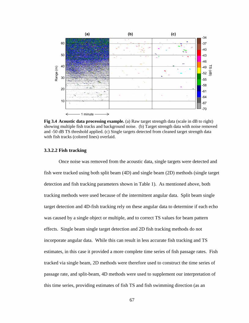
67

Fig 3.4 Acoustic data processing example. (a) Raw target strength data (scale in dB to right)

showing multiple fish tracks and background noise. (b) Target strength data with noise removed

and -50 dB TS threshold applied. (c) Single targets detected from cleaned target strength data

with fish tracks (colored lines) overlaid.

3.3.2.2 Fish tracking

Once noise was removed from the acoustic data, single targets were detected and

fish were tracked using both split beam (4D) and single beam (2D) methods (single target

detection and fish tracking parameters shown in Table 1). As mentioned above, both

tracking methods were used because of the intermittent angular data. Split beam single

target detection and 4D-fish tracking rely on these angular data to determine if each echo

was caused by a single object or multiple, and to correct TS values for beam pattern

effects. Single beam single target detection and 2D fish tracking methods do not

incorporate angular data. While this can result in less accurate fish tracking and TS

estimates, in this case it provided a more complete time series of fish passage rates. Fish

tracked via single beam, 2D methods were therefore used to construct the time series of

passage rate, and split-beam, 4D methods were used to supplement our interpretation of

this time series, providing estimates of fish TS and fish swimming direction (as an

68

indicator of tidal stage), and verifying temporal patterns in the time series made from fish

tracked in 2D. All tracks were exported for further analysis in R (3.1.1, R Core Team,

Vienna, Austria).

Table 3.1 Acoustic data processing parameters. Parameters were used in Echoview® software

to detect and track individual fish.


Single target

detection: single

beam method 2

TS threshold -50 dB




Single target

detection: split

beam method 2

TS threshold -50 dB





Max. beam compensation 12.00 dB

Max. standard deviation of:



Minor-axis angle range -2.5° - 2.5°

Major-axis angle range -2.5° - 2.5°


Alpha (range) 0.8

Beta (range) 0.5

Exclusion distance (range) 0.5 m

Missed ping expansion (range) 0 %

Weights:

Range 0

TS 0

Ping gap 0







Exclusion distance(major, minor, range) 1.5, 1.5, 0.5 m

Missed ping expansion (major, minor, range) 0, 0, 0 %

Weights:

Major axis 0

Minor axis 0

Range 0

TS 0

Ping gap 0




69

3.3.3 Data Analysis

Data analysis included time series construction, time series gap-filling, the

wavelet transform, and tidal stage modeling. The TS of fish tracked with 4D methods

was summarized with median and interquartile range, but closer examination was

avoided due to the mixed nature of the fish assemblage in Cobscook Bay and our

inability to identify the species of each detected fish.

3.3.3.1 Time series construction

The time associated with each tracked fish was used to acquire counts of fish in 1-

hr time increments, equating to a rate of fish passage through the sampled volume with

units of fish·hr-1. The distribution of ranges at which fish were detected did not change

substantially over time, so individual fish were not weighted to account for beam width.

3.3.3.2 Gap-filling

Before the time series could be used in wavelet analysis, the gaps in the data

needed to be filled by new values which would minimally impact subsequent temporal

pattern analysis. This was done by mimicking the temporal patterns of the time series to

the sides of each gap. For each gap, a Fourier transform was used to identify the most

prevalent frequencies in the data within one gap-width before and after the gap (or 48

hours, if the gap was shorter). The upper 50% of the most important frequencies were

chosen, which allowed the number of frequencies used to vary with gap size and

mimicked the nearby data well. For each set of data from before and after a gap, the

selected frequencies were used to construct a model of fish passage rate in the form:

𝑦 = ∑ 𝐴𝑖sin (2𝜋𝑓𝑖𝑡) + 𝐵𝑖 cos(2𝜋𝑓𝑖𝑡) + 𝜀

𝑁

𝑖=1

70

where y is modeled fish passage rate, fi is the ith frequency of the N frequencies selected

via the Fourier transform method, Ai and Bi are amplitudes, and ε is random error.

Coefficients A and B and residual error values were obtained by fitting a linear model of

the above form to data before and after the gap. Passage rate was predicted for each time

point within the gap using both models, the results of which were weighted and summed:

values from the before-gap model were weighted by 1-1/j, where j was the index of the

predicted data point; data from the after-gap model were weighted in an opposite fashion.

Though residual error was useful in evaluating each model’s fit, error was not added to

the predicted gap values. Introducing random error based on residuals simply

exaggerated high-frequency noise within gaps that was uncharacteristic of the rest of the

dataset, and this omission did not significantly alter results.

3.3.3.3 Wavelet transform

Once gaps in the time series were filled, a wavelet transform was used to inspect

patterns in passage rate and how they changed over time. Wavelet transforms

simultaneously decompose time series data across both the frequency and time domains

by convolving the time series with a wave form (the ‘wavelet’), which is scaled up or

down within a chosen range as it is moved along the time axis. The result is a wavelet

spectrum: a 2D representation of the prevalence of periodicities (frequency-1) that

compose the original time series, across the time spanned by the dataset (2 years, in this

case). We applied a continuous wavelet transform using the Morlet wavelet to our time

series of fish passage rate (package WaveletComp in R; Roesch and Schmidbauer 2014).

The maximum frequency included was 2 times the sampling frequency (a periodicity of 2

hours), as this would be the highest possible frequency that could theoretically be

71

characterized (i.e., the Nyquist frequency). The maximum periodicity was limited to one-

half of the total sampling period (1 year) because larger periodicities are overwhelmed by

edge effects. The wavelet spectrum was tested at a 95% confidence level against a

theoretical spectrum of white noise fit to the series using 100 iterations.

3.3.3.4 Tidal stage modeling

Fish tracked using split-beam, 4D methods were used to indicate the tidal stage

via their direction of movement. At this site, fish move almost exclusively in the

direction of the current except at slack tides, when movement was more uniformly

distributed for a brief period of time (Viehman and Zydlewski 2015, Viehman et al.

submitted). Fish direction could therefore be used as a proxy for tidal current direction,

which could indicate tidal stage. This correlation was verified by comparing predicted

tidal stages to several instances of ADCP current speed data that were collected from a

moored vessel at the same site during the study period (Fig 3.5). Shifts in fish swimming

direction (Fig 3.5a) corresponded to slack tides as indicated by the ADCP data (Fig 3.5b).

The square-wave pattern of fish movement direction was very similar to the measured

and modeled current direction at a nearby location presented by Xu et al. (2006), and

flood and ebb tide movement directions (approximately 285° and 120°, respectively)

aligned well with the known current direction at our study site (ORPC personal

communication).

72

Fig 3.5 Fish heading and current velocity. Data were collected at the TidGen® site in March

2013. (a) Individual fish heading (gray points) shown with fitted tidal model (solid line) and its

midline (horizontal line), which were used to calculate times of slack tide (vertical dashed lines).

(b) Current speed collected concurrently by an ADCP at the same site, with same times of slack

tide as shown in (a).

As large gaps existed in the 3D acoustic data, and therefore in the swimming

directions available for tidal stage assignment, a tidal model was fit to existing fish

direction data which could then be used to accurately predict tidal stage, even when 3D

data were missing (thick solid line in Fig 3.5a). This tidal model was a summation of

multiple sinusoids with varying periodicities, including the ten tidal components that

have been used in shorter-term modeling studies of Cobscook Bay tidal currents (M2,

K1, K2, N2, S2, O1, L2, M4, NU2, 2N2; Rao et al. 2015) and five other tidal

periodicities that would be relevant to this 2-year span (P1, Q1, MF, MM, SSA). The

73

model was constructed as for the gap-filling step, except in this case fi was the ith tidal

frequency of the 15 tidal components listed above (frequency = period-1). Amplitudes A

and B were obtained by fitting a linear model of the above form to the available fish

direction data from the 3D dataset. The sinusoid peaks were defined as peak flood tides,

the troughs were peak ebb tides, and slack tides (high or low) occurred wherever the

sinusoid crossed its midline (Fig 3.5a).

3.4 Results

3.4.1 Target strength

The median target strength estimated from fish tracked using the 4D method was -

45.1 dB, with an interquartile range of -46.5 to -43.4 dB. Using Love’s (1971) general

TS-length equation, this corresponds to a median fish length of approximately 6 cm, with

an interquartile range of 5 to 7 cm.

3.4.2 Time series

Passage rates determined through 2D and 4D tracking methods agreed well with

each other (Fig 3.6). Counts obtained via 2D methods were slightly higher than those

obtained using 4D methods due to the less stringent target quality requirements of 2D

tracking (Fig 3.6a), but when data were available in both datasets, the patterns were the

same (Fig 3.6b).

74

Fig 3.6 Comparison of fish passage rates obtained via 2D and 4D tracking. (a) 4D rates vs.

2D rates, shown with 1:1 line. (b) Subset of 2D (solid line) and 4D (dashed line) passage rates

from October 2014.

Fish passage rate varied greatly over the two years spanned by the dataset, on

both short and long time scales (Fig 3.7a). Overall, passage rate was highest in late

summer and fall of both years, reaching over 1000 fish·hr-1. During winter and spring,

rate maxima were in the hundreds of fish·hr-1. Passage rate could increase from 0 to

hundreds of fish·hr-1 in a matter of hours, and it was evident that this variation was cyclic

in nature (Fig 3.6b, Fig 3.7a). Values generated to fill the 20 gaps that existed in the 2D

dataset appeared consistent with patterns in the surrounding data (Fig 3.7a) and were

unlikely to interfere with interpretation of the wavelet spectrum.

3.4.3 Wavelet transform

The wavelet transform (Fig 3.7b) revealed the presence of a 365-day periodicity,

which is indicative of the seasonal cycle that was evident in the raw time series (Fig

3.7a). This seasonal change in passage rate slightly lagged the seasonal change in

temperature, with lowest rates in between winter and spring (e.g., March) and highest

75

rates in the fall (August through November). A continuous band in the wavelet transform

at the 183-day periodicity and fainter, less continuous bands at around 14 and 28 days

were also present, and coincided with tidal periodic components (Rao et al. 2016).

The strongest features of the wavelet transform were bands near 12- and 24-hr

periods, which indicated variation in fish passage rate related to the tidal (and/or semi-

diel) and diel cycles. These two periodicities were not constant throughout the dataset,

but followed similar patterns in every year sampled, though with some variation in

timing. The 24-hour periodicity was present only in the summer and fall, emerging in

June in 2014 and 2015. The 12-hour periodicity was present throughout the year, but was

most evident in the winter and spring (from January through May). For the rest of the

year, the 12-hr periodicity was present but intermittent.

76

Fig 3.7 Fish passage rate time series and wavelet analysis. (a) Time series of fish passage rate

(fish·hour-1). Gaps in data that were filled using the method described in the text are shown in

gray. Inset expands time series from July 2014. (b) Wavelet transform of log-transformed time

series. Color indicates the magnitude of the wavelet power, with darker, redder colors indicating

higher power. Black contours enclose areas of significance at the 5% significance level. The

transparent white fill indicates the cone of influence, within which power values may be reduced

by edge effects. Darkened rectangles indicate where gaps in the time series were filled. (c) Fish

passage rates during each hour of each day of the time series, condensed here for easy

comparison to a and b. An expanded version of c is shown in Fig 3.8. Darker, redder colors

indicate higher passage rates. Horizontal curved lines indicate times of sunrise and sunset, and

shaded rectangles indicate filled gaps in the time series.

77

Visual inspection of passage rate at each hour of the day (Fig 3.7c) revealed

obvious changes in passage rate that corresponded with the presence and absence of 12-

and 24-hr periodicities in the wavelet transform. When viewed in relation to tidal and

diel stage (Fig 3.8), it was clear that fish passage rate varied with tidal and diel cycles in a

seasonally shifting relationship. In the winter and spring of each year (from January

through May), when the 12-hr periodicity was present but not the 24-hr, the highest rates

occurred on the second half of the ebb tide and at low tide, mainly near sunrise and sunset

but with no strong difference between day and night. In the summer (June through

August), when both the 12-and 24-hr periodicities were evident, the highest passage rates

began shifting to night and were still mostly associated with low tide, though sometimes

in the second half of ebb or first half of flood. In the fall and early winter (September

through December), the 24-hr periodicity became more prominent while the 12-hr

periodicity became less consistent. At this time, passage rate was clearly higher at night

than during the day, and the association with tidal stage was less clear, though the rate

was generally lower at high tide than at ebb, low, and flood tides. Between December

and January, this pattern in passage rate quickly returned to peaks at low or ebb tides at

sunrise and sunset.

78

Fig 3.8 Fish passage rate at each hour of the day. Rows correspond to hour of day, columns

correspond to day within the time series, which spans July 2013 to July 2015. Darker, redder

colors indicate higher passage rates. Gaps in the time series (filled using method described in

text) are indicated by darkened rectangles. Horizontal curved lines indicate time of sunrise and

sunset. Points indicate times of low (open circles) and high (solid circles) slack tides. A

condensed version of this figure is shown in Fig 3.7c.

79

3.5 Discussion

This high-resolution, long-term time series indicated that fish passage rate was

highly variable and strongly linked to multiple cyclic changes in the physical

environment, including tidal, diel, and seasonal cycles. This is not surprising, given the

high-magnitude seasonal shifts and tidal forcing at this site, and that fish movements have

been linked to such environmental changes in previous studies (Pittman and McAlpine

2001). The passage rate of fish varied most with tidal and diel cycle, but its relationship

with these cycles did not remain constant over a year. Rate was linked strongly to the

interaction of these two cycles in a relationship that varied with season. This adds to

previous findings linking similarly interacting environmental cycles with fish presence

and feeding in intertidal habitats (Krumme et al. 2008, Gibson et al 1996) and spatial

distribution of fish and their predators and prey in tidal current systems (Simard et al.

2002, Embling et al. 2012, Zamon 2003).

All interactions of fish passage rate with the tidal cycle were modified by the diel

cycle. In the winter through spring, the highest passage rates were confined to low slack

and ebb tides, but within crepuscular periods. Higher rates shifted into night during the

summer, expanding to flood and ebb tide in addition to low slack tide and remaining this

way through the fall. These results are consistent with a previous study we carried out at

this site, in which we conducted 24-hr surveys of fish density and vertical distribution

using a downward-looking, vessel-mounted echosounder in March, May, June,

September, and November 2011 (Viehman et al. 2015). In that study, we did not

examine slack tides. However, we found that fish density was generally higher during

the ebb tide than the flood tide in the first part of the year, and that this difference was

80

less evident toward the end of the year. The vertical distribution of fish did not differ

consistently between ebb and flood tide, so higher ebb- or flood-tide passage rates may

be related to horizontal, rather than vertical, tidal fish movement. For example, fish may

move between channel edge habitats and the middle of the channel based on flow

direction, or be carried through different parts of the channel during ebb and flood tides

on asymmetric flow paths.

The diel differences in passage rate which we observed, on the other hand, could

have been related to changes in vertical fish distribution. Unlike tidal stage, our previous

study of this site found consistent changes in fish vertical distribution related to diel

stage: during the day, fish were more concentrated near the sea floor or surface,

depending on time of year, but at night, fish spread out in the water column (Viehman et

al. 2015). In that study, this difference was visually apparent in May, June, August, and

September surveys, but not in March. In the present study, we sampled only the mid- or

lower-water column (depending on water height). So, if the same diel shifts in vertical

distribution were occurring during the present study period, from spring through fall most

fish would have been outside of our sampled volume during the day but would have

moved within view at night, and there would be little day-night difference in passage rate

in the winter and early spring. This is consistent with our results, with higher passage

rates occurring at night from June through December. However, the influence of diel

cycle was not completely lacking in the winter and early spring, as passage rate

consistently peaked near dawn and dusk when those times coincided with low or ebbing

tides. Our previous work only compared day- and night-averaged vertical distributions,

so we had not captured any changes in fish activity related to dawn and dusk. By

81

expecting and searching for 24-hr diel differences in fish distribution at this site, we did

not detect this crepuscular activity pattern that dominated for a large portion of the year.

Prior assumptions such as this have likely constrained results in other studies of fish

biology, as well (Heath et al. 1991), highlighting the utility of long-term, high-resolution

data collection.

It is important to remember that only individual fish were included in this study,

as individuals within schools could not be separated from their neighbors, and fish

schools often could not be distinguished from patches of entrained air. Fish in schools

were therefore omitted, which potentially affected the patterns in passage rate we were

able to measure. For example, we previously observed that many dense schools are

present in Cobscook Bay in the spring (Viehman et al. 2015, unpublished data), likely

larval Atlantic herring (Clupea harengus, Vieser 2014). These schools contributed to

high density indices in spring that were comparable to indices from the fall (Viehman et

al. 2015, unpublished data). However, in the present study, passage rates in the spring

were much lower than in the fall, which could have been due to the exclusion of these

schools. Individually, larval herring may not be strong enough acoustic targets to be

tracked with a -50 dB TS threshold, so even if schools were to spread out (e.g., at night;

Heath et al. 1991, Ferreira et al. 2012), they would be unlikely to contribute to fish

passage rate. However, many schooling fish species have been observed to spread out in

lower light levels, including adult Atlantic herring (Blaxter 1985) and Atlantic mackerel

(Scomber scombrus, Glass et al. 1986), both of which would be detectable above our TS

threshold. These fish are present in the area in high numbers in the summer and fall

(Vieser 2014, MacDonald et al. 1984), when the diel pattern in passage rate was

82

strongest. It is possible that the diffusion and formation of schools of fish, such as

herring and mackerel, could have influenced the observed passage rates. Ideally, schools

would be included in this study, but to do so, new processing techniques to separate

schools of fish from entrained air need to be developed.

Hydroacoustics could not reveal the species of fish at this site, but physical

sampling that occurred from 2011 to 2014 (Vieser 2014, Zydlewski et al. 2016) indicated

which species were likely present. These studies sampled the tidal channels of the bay

with pelagic and benthic trawls and the intertidal areas with seine and fyke nets from

spring to fall of each year. They found that Cobscook Bay has a diverse fish assemblage,

with 46 species sampled, many of which have seasonal in- and off-shore movements in

the Gulf of Maine (Bigelow and Schroeder 2002, Tyler 1971). Atlantic herring and

winter flounder (Pseudopleuronectes americanus) were by far the most abundant species

caught in the tidal channels, making up 59.6% and 27.1% of the catch (Vieser 2014).

Most fish sampled were juveniles, with lengths agreeing well with the TS of fish detected

in this study. Some larger fish were also likely present and able to avoid the trawls, such

as adult Atlantic mackerel in the summer and fall. Four diadromous species, which have

well-defined annual on- and off-shore movements related to spawning, were also

captured: alewife (Alosa pseudoharengus), rainbow smelt (Osmerus mordax), blueback

herring (Alosa aestivalis), and American eel (Anguilla rostrata). The life stages of some

of the fish species sampled were also found to change seasonally: herring sampled in

May and June were typically larval, while those sampled in August and September were

juvenile or adult. Some of the patterns we observed could have been related to fish

growing into the size ranges we sampled by setting a -50 dB TS threshold. For example,

83

while individual larval herring (not schooling) may be too weak to detect, juvenile

herring several cm long would likely be strong enough targets. If larval fish remain in

Cobscook Bay and mature over the course of the spring and summer, their growth could

contribute to the comparably higher passage rates observed in summer and fall.

The changing patterns in fish passage rate that we observed each year are also

likely related to the seasonally changing fish assemblage of Cobscook Bay. Vertical and

horizontal movement patterns of fish in response to environmental cues are often specific

to species and life stage (Pittman and McAlpine 2001, Neilson and Perry 2001), and can

change seasonally even for one species as fish respond to changing day length and

temperature (Gibson et al. 1996). Though the vertical diel and tidal movements of most

of the species present in Cobscook Bay (Vieser 2014) are not well known, particularly in

such fast flows, a seasonally shifting fish assemblage is likely to result in seasonally

shifting patterns in passage rates, such as those we observed. The presence of herring

and mackerel in the summer and fall, for example, could have substantially contributed to

the increase in night-time passage rates, e.g. due to school diffusion (Blaxter 1985, Glass

et al. 1986) or diel vertical migrations (Huse and Korneliussen 2000, Nilsson et al. 2003)

bringing more individuals into the sampled volume. Without the ability to separate

acoustically detected fish by species, the unique movement pattern of any one species at

this site is virtually impossible to separate from the combined movement patterns of all

the others. In future studies of regions with diverse fish assemblages, it may be helpful to

collect data with multiple acoustic frequencies to aid in distinguishing anatomically

distinct groups of fish (Korneliussen and Ona 2004).

84

In the present study, we saw no consistent correlation between fish passage rate

and current speed, and this has implications for potential MHK device effects. Previous

work by Broadhurst et al. (2014) and Hammar et al. (2015) used video to observe fish

interacting with MHK turbines at two other locations, and both studies concluded that

fish were less abundant at high current speeds and therefore less likely to come in contact

with moving turbine blades. This or any other consistent response to the tidal currents at

our study site would have appeared in the wavelet transform as a strong band near the 6-

hr periodicity, which was not the case. Instead, we observed that passage rate was

frequently high during the flowing tides (not only at slack tides), particularly at night

from summer through fall. If passage rate is assumed proportional to rate of encounter

with an MHK turbine at the same depth, fish may be more likely to contact moving

turbine blades than might be expected based on results of previous studies, particularly if

combined with the finding by Viehman and Zydlewski (2015) that fish were less likely to

evade an MHK turbine at night than during the day. However, this speculation should be

balanced with the results of laboratory studies of fish entrained in MHK turbines, which

found survival rates generally exceeded 90% (Amaral et al. 2015, Castro-Santos and

Haro 2015). So, even if the rate of fish encountering and entraining in the MHK turbine

is high, the magnitude of direct turbine effects such as blade strike may still be minimal.

This is particularly true for small fish, such as those detected here: as fish size relative to

blade diameter decreases, injury and mortality have also been found to decrease (Amaral

et al. 2015).

The high temporal variability in fish passage rate also has implications for

monitoring the effects of tidal energy turbines on fish. For example, to monitor near-field

85

interactions of fish with an MHK device (e.g., direct strike by turbine blades), it would be

best to focus sampling efforts on times with high passage rates and a rotating turbine. At

this site, the best time to observe turbine interactions in the winter and spring would be

near sunrise or sunset during the second half of ebb tide, and in the summer and fall, at

night during either flood or ebb tide. Consideration should be given to the fish species

and life stages that would be present at different times of the year, as they may all

respond differently to an MHK device.

One approach to quantifying less direct MHK device effects is to monitor fish

abundance in the area of a device before and during its deployment (Viehman and

Zydlewski 2015, Staines et al. 2015). Unless monitoring can be continuous, as in this

study, the high temporal variability in fish presence in such dynamic environments could

influence results of long-term studies if they are not designed to consider these cycles.

This must be kept in mind when interpreting results from tidal energy sites. For example,

if our echosounder were duty-cycled to collect data for just a few hours of the month (and

therefore reduce processing and analysis time substantially), samples occurring at low

tide would be capturing higher passage rates relative to samples occurring at high tide.

The timing of observations in relation to underlying cycles in fish presence, which are

based on the environment and the behavioral responses of fish, could alias results and

produce trends that are not actually there. It is important that results of such monitoring

reflect actual trends in fish abundance. Overestimating effects on fish could harm this

developing industry but underestimating effects could harm the marine ecosystem.

Carrying out 24-hr surveys, which capture the high variation occurring over 12- and 24-

hr cycles, spaced over time to characterize the seasonal cycle each year, would be a first

86

step toward achieving accurate long-term monitoring results at tidal energy sites like this

one. As more data are collected in the coming years, longer environmental cycles (e.g.,

climatic oscillations) will need to be taken into account, as they may also influence

observed trends. This long-term variation would be difficult to characterize without

studies spanning decades, but sampling a control or reference site alongside a tidal energy

site would aid in separating this and other sources of natural variation from effects of

MHK devices.

Results presented here are specific to one depth at one site, but they may be

applicable to other tidal energy sites characterized by similarly high-magnitude

environmental cycles. In strongly tidal channels frequented by valuable or endangered

fish species (e.g., salmon in the northwest USA or Atlantic sturgeon in the northeast),

observing passage rates with high temporal resolution could be very useful in predicting

and mitigating MHK device effects. Fish passage rates at turbine depth could be

combined with observations of close-range evasion behavior in the field, as well as fish

injury and mortality rates obtained in laboratory settings, to estimate the effects of a

single turbine on the fishes sharing its depth. When continuous or high-frequency

sampling is not an option, known environmental cycles should be used to inform plans

for monitoring turbine effects on fish, as well as the interpretation of study results. Better

understanding of the effects of a single MHK device on individual fish may help us

predict the effects of devices on fish populations as this new renewable energy industry

moves toward the deployment of commercial-scale MHK device arrays.

87

CHAPTER 4

INCORPORATING ENVIRONMENTAL CYCLES INTO STUDY DESIGNS

IMPROVES FISH MONITORING AT TIDAL ENERGY SITES

4.1 Abstract

Continuous, long-term (multi-year) monitoring of animal presence at tidal energy

sites may be the ideal approach for separating cumulative effects of marine hydrokinetic

(MHK) devices on biota in a region from natural variability, which is high in these areas.

However, continuous sampling is often unrealistic due to cost or gear limitations, and

discrete sampling must be used instead. Fish presence at tidal energy sites is tied to

environmental changes, which are often cyclic in nature (e.g., tidal, diel, and seasonal

cycles). The timing and duration of discrete samples can therefore greatly affect

observed trends. Timing discrete samples to account for the cyclic patterns in fish

presence at a tidal energy site may improve the quality of long-term monitoring results

and reduce costs of monitoring by avoiding the need for high-frequency or continuous

sampling. We explored this idea by subsampling a two-year continuous time series of

fish passage rate at a tidal energy site in Cobscook Bay, Maine. We simulated the use of

different study designs at the site and compared their ability to capture the seasonal trend

in passage rate. Designs used either randomly spaced samples or samples informed by

environmental cycles which held the relevant environmental conditions constant (e.g.,

tidal, diel, and lunar stages). Sample durations simulated were 1, 12, and 24 hours, and

frequencies ranged from 3 to 12 per year. The temporal representativeness of each

sample duration ranged from 72 hours for 1-hr samples to 44 days for 24-hr samples.

Informed designs using 24-hr samples were the most accurate, efficient, and correlated

88

with the true seasonal trend in fish presence. Sample duration had the largest effect on

design quality, and at least 4 samples per year were required to best reflect the true

seasonal trend. This approach to study design for detecting MHK device effects may be

applicable to tidal energy sites around the world, where similar environmental forcing

exists. As patterns in fish presence will vary with fish assemblage, the species and life

stages of fish present at each tidal power site should be considered when using this

approach to inform study design.

4.2 Introduction

Baseline information on biological systems is important for the prediction,

detection, and understanding of anthropogenic influences (Smith et al. 1993). Even with

baseline information, detecting effects in the natural environment can be difficult due to

natural variation affecting data collected before and after a site is perturbed. A before-

after-control-impact (BACI) study design can aid in separating natural variation from

effects of an anthropogenic change (Smith et al. 1993, Osenberg et al. 1994). Under this

design, discrete samples are taken at the impact site before and after the perturbation is

made, as well as at a control site that experiences the same natural variation but is not

impacted by the same change. By comparing before to after at each site, effects of

anthropogenic changes may be separated from any natural variation. The ability of a

BACI design to detect impacts relies heavily on the number of samples taken before and

after the change is made, the natural variability of the parameter measured, and the size

of the effect (Osenberg et al. 1994). Without enough baseline information, it can be

difficult to determine the number of samples needed prior to the change being made.

Additionally, BACI comparisons do not necessarily require understanding of the natural

89

variability to separate it from the effect of interest, but the natural variation may be

critical to understanding the mechanisms driving the effects and predicting future effects

as anthropogenic perturbations scale up or change in some other way.

Without some understanding of the variation in a biological quantity of interest

prior to designing a study, results may be inaccurate or incomplete. For example, the

interaction of short-term patterns with longer-term changes, such as diel and tidal

movements with the seasonal cycle, can limit the scope of results if not taken into

account. Viehman et al. (2015) took discrete 24-hr measurements of fish vertical

distribution several times per year for two years, and compared day- and night-averaged

distributions. They found that fish were concentrated near the sea floor or surface during

the day and were more spread out at night, except in winter, when there was no sign of a

diel difference. However, continuous data collection over two years (Chapter 3) revealed

high fish passage rates mid-water-column during the crepuscular periods in the winter, a

semi-diel pattern that was not seen in the previous study due to prior assumptions about

diel fish movements. Both of these studies were carried out to inform predictions of the

effects of a marine hydrokinetic (MHK) device on fish and provide a baseline of

comparison for data collected post- device installation. As such, it was important that

study results accurately represented fish presence at the site, as this largely determines the

potential rate of fish encounter with an MHK device.

Fish behavior, and therefore presence at any particular location, vary with species

and life stage, the needs of the individual (e.g., feeding, migrating, spawning), and

environmental conditions (e.g., light, currents, temperature, and day length; Pittman and

McAlpine 2001, Reebs 2002). In dynamic, variable environments such as tidal energy

90

sites, metrics of fish abundance (e.g., density or passage rate) are similarly highly

variable (Viehman et al. 2015, Chapter 3). In such a setting, study design can greatly

influence results if the natural variation is not understood well enough to inform the

monitoring plan. For instance, the number of samples needed to fully characterize the

quantity of interest (e.g., fish passage rate) and to detect any change is dependent on its

variability. Under-sampling provides too little information to draw accurate conclusions,

but over-sampling can waste limited resources. To optimize sample frequency and

duration for specific research goals, the temporal representativeness of a data point, i.e.

how much time is represented by the results of a single sample (Jacques and Horne 2014,

Anttila 2012) should be defined.

The timing of each individual sample within a study is also important, particularly

in areas where the quantity of interest is cyclic in nature. This is because the interaction

of sampling frequency with the underlying cycles can generate false patterns in the

resulting dataset (e.g., signal aliasing, Vaseghi 2008). Many of the environmental

conditions that affect fish activity and movement are cyclic (e.g., diel, lunar, and seasonal

cycles), and tidal areas are subjected to the additional influence of the various periodic

components of the tidal cycle (Gibson 2003). Fish passage rate at a tidal energy site in

Cobscook Bay, Maine was strongly influenced by tidal, diel, and seasonal cycles

(Chapter 3), and this is likely to be the case in many areas with environmental forcing of

similar magnitude. The best method for characterizing this type of highly variable, cyclic

quantity would be to collect high-resolution data (e.g., sample at several times the

shortest frequency present) for a long period of time (several times the period of the

longest cycle present). One method for sampling large volumes of water at very high

91

temporal resolution is hydroacoustics. Hydroacoustic equipment can be deployed

remotely and operated for long periods of time, making it suitable for high-resolution,

long-term data collection (Flagg et al. 1994, Cochrane et al. 1994, Picco et al. 2016,

Jacques and Horne 2014, Urmy et al. 2012). However, remote deployments are costly to

build and deploy, and they are limited by battery life if not cabled to shore. Additionally,

acoustic data generally require large amounts of digital storage space and time-

consuming manual processing. For a start-up company monitoring the effects of an

MHK device on fish with limited resources, more realistic options might include discrete

hydroacoustic samples spread out over time (e.g., vessel-based transects at a site), or

duty-cycling a remotely deployed echosounder (to extend battery life, reduce data

storage, and limit processing time).

If continuous sampling is not an option, incorporating the cyclic nature of fish

presence at a tidal energy site into monitoring plans may be advantageous. Several

studies of the temporal variability in the marine realm have suggested such incorporation

of natural patterns to improve the accuracy of study results (Embling et al. 2012, Blauw

et al. 2012). Even without a thorough baseline, if the dominant environmental

periodicities at a tidal energy site are known, the dominant cycles in fish presence may be

inferred. The research question can then determine which cycles are important to

characterize, and which are not necessary to characterize but could influence observed

trends. The cycles to be characterized would set the minimum desired sampling

frequency (several times the frequency of the shortest cycle of interest) and the minimum

total time spanned by the study (several times the length of the longest cycle of interest).

Cycles influencing the results that are not of interest can then inform the duration and

92

spacing of individual samples. This technique has been used in water quality monitoring

to remove the effect of diel and seasonal cycles on long-term chlorophyll-a measurements

when seasonal and diel cycles were of less interest than multi-year trends (Anttila 2012).

By sampling a station during the same seasonal event each year, the influence of seasonal

cycle is avoided, and by sampling for an entire day and obtaining the day’s average, the

influence of diel cycle is removed (Anttila 2012).

The same method may be applicable to measurements of fish presence at tidal

energy sites. A general monitoring goal is to characterize fish presence at a site before

and after an MHK device is deployed, in order to detect cumulative device effects. The

temporal scale at which these effects occur is not yet known, and is likely to vary based

on the stressor (e.g., noise, direct strike) and receptor (e.g., different fish species or life

stages) (Boehlert and Gill 2010). To examine the longer-term effects of device operation,

a study should be designed to detect changes occurring over months and years, rather

than days (which may be more appropriate for monitoring transient effects of device

installation activities). This suggests a sampling frequency of several times per year,

particularly if a seasonal cycle is present. Next, sample duration and timing must be

decided. If sample duration is a multiple of a cycle’s period, summary statistics of the

sample (e.g., mean or median) can be used to cancel out that cycle’s effects. For

example, the influence of short-term cyclic variation caused by the tidal or diel cycles

(periods of 12 and 24 hr, respectively), could both be removed from the longer-term

observations by setting sample duration to 24 hr. Any intermediate cycles, which have

periods longer than sample duration and frequencies higher than sample frequency (e.g.,

the lunar cycle), must be accounted for with sample timing. For example, if 24-hr

93

samples are carried out at a sampling frequency of 6 per year, the effect of lunar cycle

(which has a period of 29.5 days and a frequency of 12 per year) could be limited by

timing each of the 6 samples to occur at the same lunar phase.

In this paper, we explored the influence of different study designs on observed

temporal trends in fish passage rate at a tidal energy site. We did this by subsampling a

two-year time series at an MHK turbine in Cobscook Bay, Maine (Chapter 3). We

simulated study designs that used various sample durations (1, 12, and 24 hrs),

frequencies (3 to 12 times per year), and timing (random, or informed by temporal

cycles). Study designs were judged based on their ability to accurately portray the

seasonal trend in fish abundance, which was the longest cycle detected in the 2-year time

series. Design quality was assessed using three metrics: accuracy, efficiency, and

correlation. Accuracy measured the departure of study results from the true seasonal

trend. Efficiency measured the effect that changes in sample timing had on results:

ideally, a good study design would not be strongly affected by slight changes in sample

timing. Correlation measured the similarity of the trend obtained via the study design

and the true trend: whether they showed similar relative changes over time, regardless of

absolute differences (accuracy). In addition, we evaluated the temporal

representativeness of samples of each duration, to provide a theoretical minimum sample

frequency (i.e., number of samples per year) required to fully characterize fish presence

at this site, and to better inform interpretation of future sample results.

94

4.3 Methods

4.3.1 Data

The data used were collected from July 15, 2013 to July 28, 2015 by a side-

looking, 7° split beam echosounder mounted on the sea floor at a tidal energy site in

Cobscook Bay, Maine (Fig 4.1; Chapter 3). The echosounder used a frequency of 200

kHz, a pulse length of 0.256 ms, and a transmit power of 120 W, and sampled

approximately 5 times per second. After noise removal, a target strength threshold of -60

dB was applied to hydroacoustic data to eliminate echoes unlikely to be from fish. Fish

were tracked, exported from Echoview®, and compiled into a time series with 1-hr

resolution. Further details of the hydroacoustic data processing and time series

construction can be found in Chapter 3. The resulting time series was the number of fish

detected within the acoustic beam each hour, or fish passage rate in units of fish per hour,

for two years.

95

Fig 4.1 Study area and echosounder setup. In lower panel, tidal current moves out of page

during the ebb tide and into the page during the flood tide. Figure components from Chapter 3.

4.3.2 Study design simulations

We simulated different study designs by sub-sampling the time series of hourly

fish passage rate. We chose to focus on accurately measuring the seasonal trend in fish

passage rate, which was the longest periodic signal present in the available time series.

The “true” trend in fish passage rate to which we compared simulation results was

obtained by applying a moving median to the time series, using a window length of 61

96

days (Fig 4.2). The median portrayed the general trends in passage rate more accurately

than the mean, which was heavily influenced by the periodic peaks in passage rate.

Fig 4.2 Time series of fish passage rate. Time series presented in Chapter 3. Gray line is raw

data, thick black line is the moving median showing seasonal variation. (a) Full time series, with

vertical black lines indicating 20-day subset shown in (b).

Three sample durations likely to be considered for long-term monitoring at tidal

energy sites were tested:1 hr (e.g., a transect or two across a narrow tidal channel), 12 hr

(to encompass a complete tidal cycle), and 24 hours (to encompass the tidal and diel

cycle; e.g. Viehman et al. 2015 and Staines et al. submitted). All samples were assumed

to be either stationary or occurring over a small spatial scale, as the spatial distribution of

fish is highly variable and likely difficult to extrapolate beyond a few hundred meters

from the point of measurement (Jacques and Horne 2014).

For each sampling duration, two study design types were simulated. These were

either “random” or “informed” by the environmental cycles known to be present and

influential to fish presence (Table 4.1) Simulating these study designs consisted of

97

dividing the year into equal time segments based on the number of samples to be carried

out, and placing one sample within each of these segments. Random designs placed

samples randomly within each segment. Informed designs randomly placed the first

sample within the first time segment, then held the relevant environmental conditions

constant for each following sample. Environmental cycles known to be influential to fish

passage rate at this site were tidal, diel, and lunar cycles (Chapter 3). For the 1-hr sample

duration, this meant selecting a data point within each segment at the same tidal stage

(ebb or flood), same part of the tide (beginning, middle, or end), same diel stage (day or

night), and same lunar phase (29.5 days apart) as the first, randomly-chosen sample. The

12-hr sample duration ensured the same diel stage and lunar phase, and began and ended

at the same tidal stage and portion of the tide, as the first sample. The 24-hr sample

duration, the length of which encompassed tidal and diel stages, held lunar phase constant

and started and ended at the same tide, portion of tide, and diel stage as the first sample.

The maximum sampling frequency attainable for informed study designs was 12 samples

per year, due to the need to hold lunar phase constant across the entire study. Sample

frequency was therefore varied from 3 to 12 for each study design to assess its effect on

results.

Table 4.1 Summary of simulated study designs.

Study

design type

Sample

duration

Sample timing

Random 1 hr Random within each time segment

12 hr Random within each time segment

24 hr Random within each time segment

Informed 1 hr Constant tidal stage, diel stage, lunar stage, and part of tide

12 hr Constant diel and lunar stages

24 hr Constant lunar stages

98

Each study design was simulated 500 times, with a different random starting time

chosen within the first time segment for each simulation. Using these multiple

simulations, we calculated the three metrics of design performance: accuracy, efficiency,

and correlation.

Study design accuracy was defined as the average percent error of each

simulation’s results compared to the true median fish passage rate. For each simulation

of a study design, the difference between each sample’s median (or single value, in the

case of the 1-hr sample duration) and the true median passage rate for the same time

frame was calculated. This number was normalized to the true median to represent error

as a percentage. The percent errors for all simulations were then averaged to calculate

the design’s overall accuracy. Larger values indicated greater error, and therefore less

accurate results for a given study design.

Study design efficiency indicated how sensitive results were to changes in sample

timing. The metric for efficiency was average coefficient of variation, 𝐶𝑉̅̅ ̅̅ , which was the

average of the CV’s of all simulated samples within each time segment. A larger value

of 𝐶𝑉̅̅ ̅̅ indicated greater variation across simulations of a given study design, and

therefore lower study design efficiency.

Correlation of sampled passage rate and the true median passage rate (e.g.,

whether the same relative changes were shown in each dataset) was quantified for each

study design using the adjusted correlation coefficient (𝑅𝑎2). For each simulation of a

study design, sampled passage rate was linearly regressed onto the true median passage

rate from the corresponding time bins (with both datasets log-transformed to meet

normality assumptions). Once all simulations were complete, 𝑅𝑎2 values were averaged to

99

compute 𝑅𝑎2̅̅̅̅ , the average adjusted correlation coefficient for the study design. Higher

correlation indicated a stronger linear relationship of the sampled and true values, e.g.

changes in one reflected the changes in the other, which indicated a better study design.

The temporal representativeness, the time span to which a single data point (e.g.,

the median fish passage rate from a sample) may be extrapolated, was then determined

for each sampling duration. This was done by re-sampling the time series at each

sampling duration and calculating the median and interquartile range (IQR) of the data

within each time bin. In the case of the 1-hr sampling duration, only one data point was

selected per sample, so this was used as the median value and the IQR was not calculated.

Autocorrelation functions of the medians and IQRs were generated, and the minimum lag

at which either the median or IQR became independent at the 95% confidence level was

identified. Temporal representativeness was then calculated as twice this lag: an

individual sample could be assumed not independent, and therefore representative, of

samples within this much time either before or after. The minimum sample frequency

(samples per year) needed to fully describe fish passage rate and its variation was

calculated for each sampling duration as 1 year divided by the temporal

representativeness.

4.4 Results

4.4.1 Temporal representativeness

The temporal representativeness of a sample increased with sample duration: 1-hr

samples were representative of the 72 hr (36 hr before and after), 12-hr samples were

representative of 29 days, and 24-hr samples represented 44 days. The minimum sample

frequency needed to fully characterize median fish passage rate and its variability at the

100

site was therefore 122 per year for 1-hr samples, 13 per year for 12-hr samples, and 8 per

year for 24-hr samples.

4.4.2 Study design simulations

Visual inspection of simulation results indicated that variability across

simulations and deviation from the true median was greatest for shorter sample durations

and smallest for longer sample durations (Fig 4.3). The results of 1-hr samples, for

random and informed designs, were highly variable from one simulation to the next and

often captured passage rates far from the true median fish passage rate (Fig 4.3a, b).

Study designs using 24-hr sample duration (Fig 4.3e, f) showed much better agreement

between simulations (higher efficiency), and followed the true trend in passage rate well

(higher accuracy). Study designs with 12-hr sample duration were intermediate (Fig

4.3c, d).

101

Fig 4.3 Results of study design simulations. 50 (of 500) simulations are shown for clarity.

Random (a, c, e) and informed (b, d, f) simulations for each sample duration (1 hr, 12 hr, 24 hr),

using sampling frequency of 12 samples per year. The grey line is the raw time series and

colored lines show individual simulations (each line is one simulation). The thick black line is

the true median trend in fish passage rate.

102

Accuracy, efficiency, and correlation metrics (Figs 4.4-4.6) supported visual

examination of the results. Sample duration had a greater effect on all metrics than

sampling frequency, with longer samples outperforming shorter ones. The effect of

sample duration was particularly strong for accuracy (Fig 4.4) and correlation (Fig 4.6).

Accuracy improved with longer samples, with error decreasing from about 180% for 1-hr

samples to 65% for 24-hr samples (Fig 4.4). Efficiency increased with longer samples,

with 𝐶𝑉̅̅ ̅̅ decreasing from approximately 3.2 for 1-hr samples to 1 for 24-hr samples (Fig

4.5). Correlation (𝑅𝑎2̅̅̅̅ ) increased from approximately 0.35 for 1-hr samples to 0.67 for

24-hr samples (Fig 4.6).

Fig 4.4 Accuracy of simulated study designs. Accruacy (indicated by percent error) shown for

sampling frequencies from 3 to 12 per year, and for sample durations of (a) 1 hr, (b) 12 hr, and (c)

24 hr. Black indicates random design type, red is informed. Error bars indicate standard

deviation.

103

Fig 4.5 Efficiency of simulated study. Efficiency (indicated by average coefficient of variation)

shown for sampling frequencies from 3 to 12 per year, and for sample durations of (a) 1 hr, (b) 12

hr, and (c) 24 hr. Black indicates random design type, red is informed. Error bars indicate

standard deviation.

Fig 4.6 Correlation of simulated study designs. Correlation (indicated by the average adjusted

correlation coefficient) shown for sampling frequencies from 3 to 12 per year, and for sample

durations of (a) 1 hr, (b) 12 hr, and (c) 24 hr. Black indicates random design type, red is

informed. Error bars indicate standard deviation.

Sampling frequency affected most study designs in a similar manner, with all

designs performing the worst at the lowest frequency, 3 per year, but improving

somewhat with increased sampling frequency. However, the three quality metrics

improved only slightly from 4 to 12 samples per year. Random and informed study

designs performed similarly for accuracy and efficiency, but informed designs showed

104

noticeably higher correlation with the true trend in fish passage rate for designs using 1-

and 24-hr sample durations.

4.5 Discussion

At this tidal energy site, study design simulations indicated that informed study

designs using 24-hr sample duration provided the best results for a multi-year study

which sought to characterize the seasonal trend in fish presence. Simulated study designs

with samples duration of 24 hrs were more accurate, less dependent on sample timing,

and better reflected the true changes in fish passage rate than designs that used shorter

samples. Sample frequency was not as important to design quality as sample duration,

though higher frequencies slightly improved results. The design which provided the most

accurate results and highest correlation used at least four 24-hr samples per year, with

timing informed by the environmental cycles (timed to occur on the same lunar phase).

The general lack of improvement at frequencies higher than four samples per year

indicate that this frequency may be sufficient to characterize changes occurring on a

seasonal scale. Timing 24-hr samples with lunar phase noticeably improved correlation

of sample results with the true median fish passage rate, but did not improve the accuracy

or efficiency. As relative changes in fish presence are very important to most monitoring

goals, the lunar phase should be held constant when planning the dates of 24-hr samples.

Shorter samples showed higher error, greater dependence on sample timing, and

poorer correlation with actual trends in fish presence than did the 24-hr samples. Very

large peaks in fish abundance occur at this site on 12- and 24-hr periods (Chapter 3), so

results from samples shorter than 24 hours are likely to be influenced by extreme values.

Holding physical factors such as tidal and diel stage constant did not consistently

105

improve accuracy or efficiency of results over those of random designs. This could

largely be due to the fact that the response of fish presence to the shorter-scale

environmental cycles changes over time (Chapter 3; Pittman and McAlpine 2001, Gibson

2003). In Cobscook Bay, Maine, in the spring, passage rates were highest in the sampled

volume near dawn and dusk, while in the fall, peak rates occurred at night (Chapter 3).

Sampling only at one time of day (e.g., near dawn) for the whole year would not account

for this seasonal change in fish presence relative to the diel cycle, resulting in a trend that

would not follow the true seasonal trend. Sampling for an entire day encompasses any

shifts in abundance relative to the diel cycle, and the resulting trend would not be as

influenced by changing diel patterns.

The temporal representativeness of 1-, 12-, and 24- hr samples unsurprisingly

indicated that samples with greater duration were representative of larger spans of time.

The temporal representativeness is useful in that it can be used to set limits for the

applicability of information from individual samples. For example, one day of data

should not be assumed to represent more than the nearest 22 days before and after, and

one hour of data should not be taken to represent more than the nearest 36 hr before and

after. This information should be used to inform study designs, based on study goals, and

should be used during the interpretation of study results. The temporal

representativeness of 24-hr samples indicated that a minimum of 8 samples per year

would be necessary to fully characterize median fish passage rate and the magnitude of

its variation. At the other extreme, 121 1-hr samples per year would be needed to acquire

the same information. If only seasonal trends are of interest, as in the situation presented

here, full characterization of fish passage rate and its variation may not be necessary; this

106

was indicated by design quality leveling off at sample frequencies higher than 4 per year.

However, different study goals may require the minimum sampling frequency or higher.

For example, if the goal of a study were to quantify the immediate effects of device

deployment on nearby fish abundance, the first few weeks after device deployment may

be of the highest interest, and 1-hr samples spaced 72 hrs apart would be sufficient for

capturing median fish passage rate and its variability over that time.

The use of 24-hr samples worked well to characterize the seasonal trend in fish

passage rate by encompassing much of the influence of the tidal and diel cycle within

each sample. However, there remained a good deal of variation that was not removed

using this method. For example, the lowest percent error of the informed 24-hr samples

was approximately 65%, and was almost entirely due to over-estimating the true median

(Fig 4.3f). The highest correlation of the informed 24-hr samples was approximately

0.69, meaning the results reflected the true median relatively well but 31% of the

variation was not accounted for by their linear relationship (i.e., there were rises and falls

in the simulated study results that were not present in the true median passage rate). This

was 7% more variation explained than the best random design with 24-hr samples

(correlation of 0.62). Though informed designs improved correlation, the remaining

unexplained variation, combined with the tendency to overestimate the true median,

indicated that the median rates from 24-hr samples were still influenced by the large

peaks in passage rate related to tidal and diel stage, and potentially other sources of

variation unrelated to these cycles.

The remaining unexplained variation highlights the importance of using a control

site for comparison while monitoring turbine effects, particularly if effects may be small

107

relative to other potential sources of variation (Osenberg et al. 1994). If both sites are

monitored with discrete 24-hr samples informed by environmental cycles, the effects of

cyclic variation on the results could be substantially reduced at both sites. Minimizing

such variation maximizes the ability to distinguish MHK device effects from other

variation, and would additionally ensure data are more comparable and consistent over

time. This is encouraging, given the monitoring efforts that have so far taken place in

Cobscook Bay. Viehman et al. 2015 began collecting information for a BACI study of

the site, which was continued by Staines et al. (submitted) and could be continued when

site development recommences. These studies have always collected 24-hr samples at

project and control sites, and so have likely substantially reduced the amount of variation

that could influence their results. These sampling methods, when continued through

future MHK device deployment at this site, will likely improve the chances of detecting

device effects through BACI comparisons.

The approach to study design presented here consists of using the known

environmental cycles at a tidal energy site to inform studies of fish presence, and it is

likely applicable to most tidal energy sites around the world. Many tidal energy sites in

the North Atlantic have similar fish assemblages: for example, Cobscook Bay (Vieser

2014) has many species in common with the Bay of Fundy (Mahon and Smith 1989) and

coastal waters of the United Kingdom (Henderson and Bird 2010), and MHK devices are

being tested in both of these areas (Stokesbury et al. 2016, Broadhurst et al. 2014). For a

given study question, the same study design may therefore be applicable at all of these

sites. Even if fish assemblages vary across sites, the distribution and behavior of many

species is driven by environmental factors (Pittman and McAlpine 2001, Reebs 2002,

108

Gibson 2003). Areas with similar environmental cycles will likely find related

periodicities in fish presence, so basic knowledge of the major environmental cycles at a

site can indicate which study designs will gather the most useful information for a given

study aim. As initial site evaluations are carried out, study design can be further

informed by more detailed information on environmental variability (e.g., current speed,

direction, and temporal components; Hardisty 2007, Copping et al. 2016). Any

information on the fish assemblage can further refine the final design (e.g., are diel

differences in fish activity likely to occur? do species change seasonally?). In addition to

reducing the cost of studies by avoiding the need for continuous sampling, the consistent

use of this approach for study design at tidal energy sites would improve the detectability

of device effects on fish and comparability of results across locations worldwide.

109

CHAPTER 5

COMBINING SCALES TO UNDERSTAND EFFECTS OF TIDAL ENERGY

DEVELOPMENT ON FISH IN COBSCOOK BAY, MAINE

5.1 Introduction

The environmental effects of marine hydrokinetic (MHK) devices on the

environment are largely unquantified, mainly due to the low number of devices installed

worldwide. Fish are a key component of the marine environment, and effects on fish are

uncertain and of great concern (Copping et al. 2016, Boehlert and Gill 2010). The

possible effects of marine hydrokinetic (MHK) devices span a range of spatial scales,

from “nearfield” effects occurring within a few blade diameters of the device to “farfield”

effects occurring multiple diameters away (Copping et al. 2015). In the case of fish, a

nearfield effect may be blade strike of an individual, or fish aggregating around a

device’s structure. A farfield effect may be fish altering migration routes to avoid the

area of an MHK device or array of devices. There is also an intermediate scale between

near- and farfield, for lack of a better term, the ‘midfield,’ where effects may include

changes to the local fish assemblage, e.g., vertical distribution or abundance, in the

general area of the device.

Potential effects of MHK devices on fish also span a wide range of temporal

scales. The natural horizontal and vertical distribution of fish, and therefore their

likelihood of encountering the MHK device in the first place , are often species- or life-

stage-specific and linked to environmental factors (Seitz et al. 2011, Bradley et al. 2015).

For example, many fish species undertake seasonal migrations that could bring them to a

tidal energy site at certain times of the year (Pittman and McAlpine 2001). On a finer

110

timescale, a species at a tidal energy site may only be present at turbine depth during

certain tidal stages, when they rise into the water column to take advantage of the current

(Forward and Tankersley 2001). The sensory and swimming abilities of fish, and

therefore their ability to detect and evade an MHK device in their path, also vary with

species and life stage (Beamish 1978, Weihs and Webb 1984, Kim and Wardle 2003).

Effects of turbines on fish will therefore vary with natural temporal changes in the fish

assemblage.

More information on how fish interact with MHK devices at multiple spatial and

temporal scales is necessary to determine at which scales effects actually occur and may

be detectable (Copping et al 2015). As it is impossible to observe all potential spatial and

temporal scales of effects with one study method, studies should occur at multiple scales

to quantify and understand MHK device effects on fish (Copping et al. 2015). Several

studies have been carried out in recent years which are increasing our understanding of

fish interactions with MHK devices and helping identify new methods for observing

effects on fish at different scales.

In the nearfield domain, laboratory studies have been used to characterize fish

behavior and rates of injury and mortality when they are entrained in MHK devices

(Castro-Santos and Haro 2015, Amaral et al. 2015). These studies indicated that survival

is quite high, on the order of 90% or more, and that behavior can change upstream of

devices (e.g., down-stream moving fish may pause before passing through or by the

turbine). In a field setting, Broadhurst et al. (2014) and Hammar et al. (2013) observed

daytime interactions of fish with different MHK devices using video. Broadhurst et al.

(2014) reported that the fish observed at an MHK device in the Orkney Isles (adult

111

pollack, Pollachius pollachius) aggregated near the device at slack tide, but dispersed as

the current speed increased. Hammar et al. (2013) examined avoidance of a device in a

tropical area, and noted that different species of fish acted differently; for example,

predatory species tended to be ‘bolder’ in approaching the device than herbivorous

species. Bevelhimer et al. (2015) used a hydroacoustic camera and observed potential

vertical avoidance maneuvers by fish within 0-15 m of an MHK device in the East River,

NY, and a decrease in fish numbers when the turbine was present may have indicated fish

avoidance of the turbine’s general area.

Studies occurring over larger spatial scales (e.g. hundreds of meters from MHK

turbines, midfield to farfield) have primarily focused on describing the natural

distribution of fish to predict the probability for spatial and temporal overlap of fish and

MHK turbines. Jacques and Horne (2014) sought to characterize the natural spatial

variability of nekton distribution at a potential tidal energy site to determine the necessary

sampling resolution for adequately moniting MHK device effects. Using hydroacoustic

transects, they found that a point estimate of nekton density could be considered

representative of the nearest 300 m. This spatial representativeness suggested that to

fully characterize nekton density at the site, instruments should be deployed at densities

of 3.56 per km2. Using knowledge of natural spatial variation in nekton density was a

unique approach to optimizing study design, and it could be applied to monitoring plans

at other tidal energy sites. As measurements must often be taken at some distance from a

deployed MHK device due to safety precautions, knowledge of the spatial

representativeness of a single point estimate can also determine the maximum distance

from a device at which a measurement can be taken.

112

To understand cumulative effects of MHK devices on fish, we need to begin

linking near-, mid-, and farfield observations. For example, the natural distribution of

fish in space and time at a site relative to a turbine (mid- to far-field; Viehman et al. 2015,

Staines et al. 2015, Staines et al. submitted, Shen et al. 2016, Chapter 3) can be combined

with nearfield fish behavior when they encounter an MHK device (Viehman and

Zydlewski 2015, Hammar et al. 2013, Chapter 1) to predict fish entrainment in the

turbine. Survival post-entrainment may then be informed by laboratory studies (Amaral

et al. 2015, Castro-Santos and Haro 2015), where events such as fish strike or injury are

easier to observe.

Our work in Cobscook Bay over the past several years is an example of multiple

scales of study that have been carried out at the same site, around the same device, with

the same fish assemblage, over a number of years. In 2010, Viehman and Zydlewski

(2015a) observed fish interaction with an MHK turbine (nearfield) for 24 hours. From

2010-2013, we observed the relative density of fish and their vertical distribution at mid-

and far-field scales, and tested for effects of turbine deployment (Viehman et al. 2015,

Staines et al. 2015, and Staines et al. submitted). At the same time, from 2011 to 2013,

Vieser (2014) characterized the finfish community of Cobscook Bay (e.g., mid- to far-

field) to inform the hydroacoustic studies and provide a baseline for future comparison.

In 2013, we used mobile hydroacoustic transects to connect data from the far- and near-

fields to predict the likelihood that fish would encounter the MHK turbine (Shen et al.

2016). In 2013 and 2014, we examined fish behavior in the near/midfield of a deployed,

static MHK turbine for several weeks (Chapter 1). Last, from 2013 to 2015, we

characterized natural fish presence in the near/midfield, without the turbine present, using

113

long-term, continuous hydroacoustic data collection (Viehman and Zydlewski 2015b and

Chapters 3 and 4).

These results, gathered over multiple spatial and temporal scales, provide the

opportunity to build a more comprehensive picture of fish interactions with an MHK

device that is not available at most sites around the world. Here, those multiple studies

are used to illustrate how various scales of observation can be combined to answer

questions about MHK device effects on the local fish assemblage, and to provide

recommendations for future research and monitoring approaches at tidal energy sites.

5.2 Cobscook Bay MHK device assessment

In Cobscoook Bay, study goals arose and evolved over time based on

conversations with ORPC, regulators, and community members. These goals can be

broadly categorized as: (1) describe the near-field interactions of fish with a single

device; (2) characterize presence of fish in the area to (3) detect the long-term effects of a

single operating device on regional fish presence and abundance and (4) predict the

probability of fish encountering the turbine; and (5) use all results to inform future

monitoring efforts. Several separate studies were carried out to address these aims,

primarily using hydroacoustics, as comprehensive physical sampling could not be carried

out with the precision and resolution necessary to address our questions.

5.2.1 Nearfield interactions of fish with the MHK device

The nearfield behavior of fish around the device was quantified in two different

studies. The first occurred in 2010 and spanned 24 hrs, using two DIDSON

hydroacoustic cameras to observe fish behavior within approximately 3 m up- and down-

stream of a test turbine suspended below a barge in Cobscook Bay (Viehman and

114

Zydlewski 2015a). This study again observed predominantly small fish (10-20 cm in

length), which is in line with the physical data later collected. As with the mobile

transects over the device, we found that these fish mainly moved with the current. They

tended to enter the turbine if they were at its depth, particularly at night, and that larger

fish (>10 cm) were more likely to evade the turbine than smaller ones. Schools of fish

were also slightly more likely to evade the turbine than individuals. During this nearfield

study, the majority of fish were observed at night after the slack tide, which aligns with

patterns we observed in the two-year time series at that time of year (Chapter 3). As with

our other studies of Cobscook Bay, these results stress the need to consider the species

and life stages of fish present and their unique behaviors when predicting device effects.

The second nearfield (bordering on midfield) study spanned several weeks in the

spring of 2013 and was used to observed fish movement in the horizontal plane 7-14 m

from the static TidGen® turbine using a bottom-mounted, split beam echosounder

(Chapter 1). This study revealed that avoidance was likely occurring at those distances,

which fills in more information between the observations by Shen et al. (2016) and the

DIDSON observations by Viehman and Zydlewski (2015a). The study further indicated

that avoidance consisted primarily of small departures from the direction of the current,

which may be sufficient for device avoidance at those distances from the device.

Assuming these movements could occur in the vertical plane, as well (which we could

not observe), this type of movement by small fish could have accounted for the fact that

half of the fish within the DIDSON viewing window were already above or below the

turbine upon arrival. This avoidance was incorporated into the probability of encounter

115

model to fill in the 10 m nearest the MHK turbine, decreasing the probability of fish

encountering the turbine from 5.8% to 2.9%.

These two nearfield studies also investigated fish behavior directly downstream of

the MHK device. The DIDSON cameras revealed that fish were almost constantly

milling in the device wake. This behavior was absent in the side-looking split beam data,

indicating that the effect was likely confined to the nearest 7 m downstream of the static

turbine (this range may be different for an operating turbine). The reason for this

behavior could not be determined, but could have been related to fish purposely

sheltering in the turbine wake or being disoriented by passage through the turbine.

Regardless of the mechanism behind this aggregation, the role of an MHK turbine as a

fish aggregating device has potential implications at the ecosystem level. Piscivores like

seals, porpoises, and diving seabirds have been found to frequent strong tidal areas where

physical forcing can aggregate prey into somewhat predictable patches (Benjamins et al.

2015), and fish aggregating downstream of MHK devices could lead them into close

proximity.

5.2.2 Fish presence at the tidal energy site

Characterizing fish presence at the tidal energy site (independent of a turbine)

required combining multiple sampling methods, including physical sampling of fish in

Cobscook Bay (Vieser 2014, Zydlewski et al. 2016), monitoring fish vertical distribution

and relative density over time (Viehman et al. 2015, Staines et al. submitted, Staines et al.

2015), and describing the variability in fish presence over short and long time scales

(Chapter 3).

116

Physical sampling was required for a general understanding of the fish species

and life stages that were likely being detected in our hydroacoustic surveys. It also

provided a baseline understanding of fish present in the area for comparison to future data

collection and detection of farfield, long-term effects on the local fish assemblage. This

physical sampling consisted of benthic and pelagic trawls carried out in the inner, central,

and outer bays of Cobscook Bay, and seine and fyke nets used in the intertidal areas of

each bay, from spring to fall of 2011-2014 (Vieser 2014, Zydlewski 2016). Results

showed that Cobscook Bay has a diverse fish assemblage, with 46 species captured

(Vieser 2014, Zydlewski et al. 2016). Atlantic herring (Clupea harengus) and winter

flounder (Pseudopleuronectes americanus) were by far the most abundant species caught

in the tidal channels (sub-tidal). Most fish sampled were juveniles, with very few over

30 cm in length. Based on local knowledge, it is likely that some larger fish were also

present but under-sampled due to their ability to avoid the trawls. These included adult

Atlantic mackerel (Scomber scombrus), which are present in large numbers in the late

summer. Many of the other species detected also have seasonal presence along the coast

of Maine (Bigelow and Schroeder 2002, Tyler 1971). The most important results of this

sampling with regard to MHK device monitoring were: (1) the baseline dataset it created

for future comparisons, and (2) that most fish at this tidal energy were small, mainly

juveniles of many different species. The results of our other studies at this site should

therefore be interpreted in this context and extrapolated to sites with different fish

assemblages with care.

Cumulative effects of an MHK device on fish in the region (i.e., the mid- to far-

field) may be reflected by changes in fish presence, e.g. abundance or density. We

117

therefore began a hydroacoustic study of the vertical distribution and relative density of

fish at the tidal energy site years before turbine deployment, to establish a baseline for

use in a before-after-control-impact (BACI) study. Down-looking hydroacoustic samples

lasting 24 hrs each were carried out at the future site of the MHK device and at a control

site 1.6 km seaward, several times per year in 2010 and 2011 (Viehman et al. 2015). This

study revealed that fish tended to be in higher densities near the sea floor, though this

varied seasonally with the fish assemblage; in the spring, for example, when larval and

recently-metamorphosed Atlantic herring were present in large numbers, fish density

tended to be highest in the upper water column. At night, fish tended to spread out in the

water column. These differences in vertical distribution were the first indication that the

likelihood of fish interacting with the MHK device, and therefore its potential effects,

were not constant over time. At this site, fish would be more likely to be at turbine depth

at night, when fish were spread out in the water column, than during the day, when most

fish would be above or below the turbine.

Samples taken during the BACI study provided snapshots of fish density and

distribution over the years studied, each with high temporal resolution (24 hours at 1 ping

per second) but separated from the others by large time gaps (months). We filled these

temporal gaps in our understanding by collecting a two-year, high-resolution (hourly)

time series of fish passage rate at turbine depth using a stationary side-looking

echosounder mounted on the sea floor at the MHK device site (Chapter 3).

Unsurprisingly, we found cyclic variation in fish passage rates linked to environmental

cycles, primarily the 12-hr tidal, 24-hr diel, and 365-day seasonal cycles but also various

components of the lunar cycle. Surprisingly, fish passage rate did not appear to be linked

118

to tidal current speed in any consistent manner. This constrasts the results of Broadhurst

et al. (2014), who detected fewer fish at higher current speeds. The fish observed by

Broadhurst et al. were large adult pollack, and apparently had different responses to

changing environmental factors, such as current speeds, than did the smaller fish of the

Cobscook Bay assemblage.

The highly variable passage rate at the depth of the MHK turbine indicated that

fish encounter rate with the turbine would be similarly variable. The highest times of fish

passage rate, and therefore turbine encounter, would generally be at night in the summer

and fall, and near sunrise and sunset in the spring and winter, depending on the tidal

stage. Whichever species contribute to the high passage rates at these times would likely

be the most affected. These patterns were consistent with the snapshots captured by our

BACI baseline surveys. However, certain discrepancies between results of the two

studies have implications for future work. In the BACI study, data were collected at high

temporal resolution but processed to detect diel differences in fish density and vertical

distribution. By averaging during the day and night, we did not detect the increased

activity occurring during low or ebb tide at dawn and dusk, which was characteristic of

the winter and spring in both years of the high-resolution time series. Fine-scale

information such as this may be important information for device siting and effect

mitigation, e.g. for commercially valuable species like Atlantic salmon (Salmo salar),

which may also target certain combinations of diel and tidal stage while migrating into or

out of rivers (Smith and Smith 1997, Lacroix and McCurdy 1996). Future studies should

be careful not to limit results with insufficient temporal resolution due to prior

assumptions of fish behavior.

119

The high-resolution, long-term dataset also informed our interpretation and

continued use of the BACI study design at this site. The detailed time series allowed us

to determine that summary statistics obtained from our 24-hr surveys were likely to be

representative of the nearest 22 days, setting a limit on the time span to which survey

results may be extrapolated (Chapter 4). Furthermore, 24-hr surveys (as opposed to

shorter ones) were found to substantially reduce the amount of variation in multi-year

monitoring results, which should improve the power of BACI comparisons to detect even

small turbine effects (Osenberg et al. 1994). As more sites are developed for tidal energy

worldwide, implementing measures to reduce variation (e.g., 24 hour surveys, timed with

important environmental cycles) should be incorporated into monitoring plans from the

outset in order to improve chances of detecting and quantifying effects of MHK devices.

5.2.3 Detect the effects of operating MHK device

Our BACI surveys continued once the turbine was deployed in order to detect

turbine effects on regional fish presence (Staines et al. submitted, Staines et al. 2015).

However, only three surveys were completed while the device was in place, and these

provided mixed results regarding turbine effects on fish density (Staines et al., submitted)

and vertical distribution (Staines et al. 2015). The mixed results may have been due to

confounding factors during data collection, which included turbine state (for one survey

the turbine was rotating, for the others it was static) and construction activities (e.g. boat

traffic, divers in the water). The BACI design appeared able to detect anthropogenic

effects on fish density at the project site, supporting the design’s application in the

dynamic environments of tidal energy sites. However, more data need to be collected

120

while the turbine is present and operational to determine if normal operation has an effect

on the local fish assemblage.

5.2.4 Probability of encounter with MHK turbine

Near to midfield data collected for the BACI study also served to estimate the

likelihood of fish encountering the MHK device. The vertical distributions of fish from

surveys of the project and control sites were used to inform a probability of encounter

model (Shen et al. 2016). This model combined the vertical distributions of fish from the

24-hr stationary surveys (Viehman et al. 2015) with vertical distributions from down-

looking hydroacoustic transects starting 200 m upstream of the device and ending 10 m

upstream of it. By tracking numbers of fish at turbine depth over the 200 m approach to

the MHK device, the probability that fish upstream of the device would be at turbine

depth upon arrival was found to be approximately 5.8%. These transects provided a

much-needed link between the near- and far-field that is difficult to obtain using

stationary surveys, and which has not yet been done at other tidal energy device

deployments.

The transects also revealed that fish numbers began to decrease as far as 140 m

upstream of the MHK device. As no decrease was observed in control transects that took

place beside the device, this indicated avoidance behavior beginning as far as 140 m

upstream of the turbine. This is some of the first information on the behavioral

“footprint” of an MHK device; that is, the distance to which fish behavior may be

affected by its presence. At a distance of 140 m, the turbine would not be visible; if fish

were avoiding the device that far upstream, it may have been in response to acoustic

emissions (Popper and Schilt 2008) or hydrodynamic cues (e.g., low-frequency

121

vibrations) detected by the fish lateral line system (Bleckman and Zelick 2009). No

hydrodynamic or acoustic measurements were made concurrent to these transects.

However, information gathered previously by ORPC (ORPC 2013) showed that certain

frequencies emitted by the rotating turbine would be above background noise levels up to

277 m away. Whether this noise was within the detection range of the fish species

present remains to be determined.

5.2.5 Informing future monitoring efforts

The 2-year time series of continuous data (Chapter 3) allowed us to examine the

potential for various study designs to capture changes in fish abundance over the seasonal

cycle. Subsampling the time series to simulate these different designs indicated that the

best method for sampling fish presence (e.g., passage rate, or some other metric of

abundance or density) in this highly variable environment was to incorporate

environmental cycles into survey timing and duration. The best design at this site was to

use 24-hr surveys, as in our BACI study, that were timed with the lunar cycle. These

surveys largely removed tidal and diel variation by encompassing those cycles, and

sampling several times per year (4 or more) provided similar levels of accuracy,

efficiency, and correlation with the actual trend in fish passage rate. Our BACI surveys

(Viehman et al. 2015) were mainly carried out near the neap tide, but did not hold lunar

phase constant. Unless surveys could be carried out at higher frequencies that would

allow the effect of the lunar cycle to be characterized (e.g., surveys several times per

month), BACI results could be improved in the future by adjusting survey timing to occur

at the same lunar phase each time.

122

If shorter surveys (e.g. 1 hr or 12 hr) were used, they would introduce more

variation to results that could limit the abilities of BACI comparisons to detect device

effects. However, shorter surveys may be more applicable if shorter-scale changes are

the goal of a study; e.g., the effect of turbine installation and the corresponding

construction activities on fish presence at the site. The temporal representativeness that

we calculated for each sample duration could be used to determine the minimum

sampling frequency for a given time period to fully characterize fish passage rate

(median) and its variation (IQR). For 1-hr surveys, this would be one survey every 36

hrs, one 12-hr survey would be required every 14.5 days, and one 24-hr survey per 22

days. Sampling at the minimum necessary frequency to accurately capture the trend and

variation in fish presence can reduce the costs of a study by using resources more

efficiently while avoiding the need for continuous data collection.

We also explored the utility of single beam echosounders for providing more

accurate information on detected fish using a post-processing method called

deconvolution (Chapter 2). This method relies on statistical assumptions to correct the

final distribution of fish target strength (TS) for the effect of the beam pattern (Clay

1983). This had not been tested for a wide-angle single beam, such as the one used in our

BACI surveys. We also tested the method on a narrow-angle single beam data, which was

represented by split-beam that had not been corrected for beam pattern by the software.

We found that the method may work reasonably well for a narrow-angle single beam

with a short pulse duration (high sampling resolution), but that the method was not

sufficient for the wide-angle single beam using a long pulse duration (lower sampling

resolution). However, deconvolution requires many fish to be sampled in order to work

123

well, and it was apparent that in some 24-hr surveys there were simply not enough

individual fish present to obtain good results. This method might enable single beam

surveys at tidal power sites to provide more useful information, such as fish size and

potentially species, but only at times when many (e.g., several hundred) fish can be

detected within a survey. Single beam transducers can always provide a relative metric

of fish density (volume backscatter, Sv), which we have previously used in our 24-hr

BACI surveys (Viehman et al. 2015, Staines et al. 2015, Staines et al. submitted).

Relative fish density may be a sufficient metric if the monitoring goal is to detect changes

in fish presence at a tidal energy site.

5.3 Summary

The studies of fish in Cobscook Bay, carried out at different spatial and temporal

scales relative to the MHK device, allowed us to form a more complete picture of device

effects. Fish at the site were small (generally < 20 cm) and represented numerous

species. We observed avoidance of the device with a rotating turbine as far as 140 m

upstream by using slight movements away from current direction, and even a static

turbine appeared to elicit this type of response at least 18 m upstream (Chapter 1). The

chance that a fish upstream of the MHK device may encounter its turbine was quite

small, on the order of 5.8%, and the chance that fish would enter the turbine was even

lower, 2.9% (Shen et al. 2016). Fish directly upstream of the device at close range (e.g.

within 3 m) tended to enter the turbine rather than evade it, especially at night (Viehman

and Zydlewski 2015a). At these close ranges, larger fish may be more successful in last-

minute device evasion than smaller fish, as swimming power is directly related to length

(Beamish 1978). To better understand the fate of fish that enter the turbine, these results

124

may be combined with those from laboratory studies, which are better able to quantify

fish strike and injury (Amaral et al. 2015, Castro-Santos and Haro 2015). We also

observed that fish may aggregate in the MHK turbine’s wake (Viehman and Zydlewski

2015a), and that this effect did not appear to extend beyond 7 m downstream of the

turbine (Chapter 1). Marine mammals and diving birds are drawn to areas where prey

aggregate (such as eddies and fronts), and such downstream fish aggregations have the

potential to attract these predators to operating MHK turbines (Waggitt and Scott 2014,

Williamson et al. 2015).

Fish presence at turbine depth, and therefore their potential to interact with the

MHK turbine, varied greatly over time and was related to environmental cycles and the

species and life stages of the fish present. The most prevalent cycles in fish passage rate

were related to the tidal, diel, and seasonal cycles, but rate was not dependent on current

speed. Instead, in Cobscook Bay, fish passage rates were often highest at night, and often

during the flowing tide, which may place them at greater risk of entering an operational

MHK turbine in their path. This result is in contrast with results of Broadhurst et al.

(2014), which indicated that the fish observed (pollack) were only present near slack tide.

This difference highlights the importance of considering each tidal energy site in the

context of the fish present and their behaviors with respect to the prevailing

environmental forces, as this determines the potential for spatial overlap between fish and

an MHK (Seitz et al. 2011, Bradley et al. 2015).

The links between fish presence and environmental conditions made it possible to

use dominant environmental cycles (tidal, diel, lunar, and seasonal) to inform study

design and improve the quality of data for detecting device effects. The BACI baseline

125

dataset we have gathered to date (Viehman et al. 2015, Staines et al. 2015, Staines et al.

submitted) used 24-hr surveys, so is nearly the best-case sampling scenario at this site.

However, variation could be further reduced by ensuring these surveys are always carried

out at the same point in the lunar cycle. The BACI comparisons we have been able to

make thus far indicate that we are able to detect effects at the project site (Staines et al.

2015, Staines et al. submitted), but those effects we detected could not be attributed to

MHK device operation alone, and more data must be collected while the turbine is

present and operational before further conclusions may be drawn.

By comparing concurrently-collected single and split beam data, we also found

that narrow-angle single beam echosounders may be able to provide accurate information

on fish TS if deconvolution methods are used (Chapter 2). If monitoring questions do not

require accurate TS or position measurements of individual fish (perhaps using relative

indices of fish density, such as Sv, instead), then assessment costs may be reduced

substantially by using narrow-angle single beam echosounders rather than split beam. A

study design that incorporates the major environmental cycles into sample timing and

duration can also reduce cost by providing better-quality information with fewer samples

(Chapter 4). Finer-scale studies of fish interactions with devices would benefit from

targeting times of higher fish passage rates (e.g., in Cobscook Bay, at night during the

summer and fall; Chapter 3) to maximize the number of interactions captured in a given

observation window, and therefore extend the reach of limited project resources.

5.4 Conclusion

In Cobscook Bay, we were able to build a comprehensive picture of fish/turbine

interactions by combining studies on multiple scales. These studies were directly

126

comparable because they all revolved around the same fish assemblage and MHK device

design. The results presented here are applicable to the fish species and life stages that

were present in Cobscook Bay during these studies, but some of the general findings may

be applicable at other locations. For example, small fish tending to move with the current

may be common to most tidal energy sites, as it is likely a result of the strength of the

current relative to the swimming power of the fish, which is directly proportional to size

across all species (Beamish 1978). The reliance of turbine effects on the spatial overlap

of fish and devices, which depends on environmental conditions and the corresponding

species- and life-stage-specific behaviors of fish, will also be a common theme at tidal

energy sites.

The comprehensive approach to monitoring a device (or array of devices) on

multiple spatial and temporal scales that we used in Cobscook Bay should be used at

other sites if a more complete, generalizable picture is to be built of the effects these

devices have on fish. What we learned here can be useful for informing future studies of

other sites and fish assemblages, even if a multi-scale approach is not possible. The most

important data to collect at a site will depend on the questions being asked, which may be

influenced by the priorities of regulators and other stakeholders. We found that a BACI

study design using several 24-hr surveys per year provided information that could be

used to answer a number of questions that arose over time. Results from those surveys

were useful in detecting anthropogenic effects at the project site, and also provided

detailed information on fish use of the water column and therefore their potential for

interacting with the MHK device. Data for use in BACI comparisons at tidal energy sites

can be improved by adjusting sample timing to account for the effects of dominant

127

environmental cycles on the behavior of the fish species and life stages present. If fish

strike is a higher-priority concern than farfield effect detection, focus should be placed on

the device’s nearfield and fish behavior should be interpreted in the context of the fish

assemblage (which may change over time and between sites) and the cues emitted by the

device.

As device installations scale up, monitoring efforts will need to evolve. The

methods presented here are tailored for monitoring the near- and mid-field effects of

MHK devices on fish, but new methods will need to be developed to address farfield

effects.

128

REFERENCES

Amaral SV, Bevelhimer MS, Čada GF, Giza DJ, Jacobson PT et al. (2015) Evaluation of

behavior and survival of fish exposed to an axial-flow hydrokinetic turbine.

North American Journal of Fisheries Management 35(1): 97-113.

Anttila S, Ketola M, Vakkilainen K, Kairesalo T (2012) Assessing temporal

representativeness of water quality monitoring data. Journal of Environmental

Monitoring 14: 589-595.

Axenrot T, Didrikas T, Danielsson C, Hansson S (2004) Diel patterns in pelagic fish

behaviour and distribution observed from a stationary, bottom-mounted, and

upward-facing transducer. ICES Journal of Marine Science 61: 1100-1104.

Beamish FWH (1978) Swimming capacity. In: Hoar WS, Randal DJ, editors. Fish

Physiology, Volume VII: Locomotion. New York: Academic Press. pp.101-

187.

Benjamins S, Dale A, Hastie G, Waggitt JJ, Lea M, Scott B, Wilson B (2015) Confusion

reigns? A review of marine megafauna interactions with tidal-stream

environments. In: Hughes RN, Hughes DJ, Smith IP, Dale AC, editors.

Oceanography and Marine Biology: An Annual Review. Vol. 53. Boca Raton:

CRC Press. pp. 1-54.

Bevelhimer M, Scherelis C, Colby J, Tomichek C, Adonizio MA (2015) Fish behavioral

response during hydrokinetic turbine encounters based on multi-beam

hydroacoustics results. Proceedings of the 3rd Marine Energy Technology

Symposium. April 27-29, Washington, D.C. Available:

http://tethys.pnnl.gov/publications/fish-behavioral-responseduring-hydrokinetic-

turbine-encounters-based-multibeam. Accessed: 2016 June.

Bigelow HB, Schroeder WC (2002) Bigelow and Schroeder’s Fishes of the Gulf of

Maine. 3rd ed. Collette BB, Klein-MacPhee G, editors. Washington, D.C.:

Smithsonian Books.

Blauw AN, Benincà E, Laane RWPM, Greenwood N, Huisman J (2012) Dancing with

the tides: fluctuations of coastal phytoplankton orchestrated by different

oscillatory modes of the tidal cycle. PLoS ONE 7(11): e49319.

Blaxter JHS, Batty RS (1985) Herring behaviour in the dark: responses to stationary and

continuously vibrating obstacles. Journal of the Marine Biological Association of

the UK 65: 1031-1049.

Bleckman H, Zelick R (2009) Lateral line system of fish. Integrative Zoology 4: 13-25.

Boehlert GW, Gill AB (2010) Environmental and ecological effects of ocean renewable

energy development: a current synthesis. Oceanography 23(2): 68-81.

129

Boswell KM, Roth BM, and Cowan, Jr. JH (2009) Simulating the effects of side-aspect

fish orientation on acoustic biomass estimates. ICES Journal of Marine Science

66: 1398-1403.

Bradley PT, Evans MD, Seitz AC (2015) Characterizing the juvenile fish community in

turbid Alaskan rivers to assess potential interactions with hydrokinetic devices.

Transactions of the American Fisheries Society 144: 1058-1069.

Broadhurst M, Barr S, Orme CDL (2014) In-situ ecological interactions with a deployed

tidal energy device: an observational pilot study. Ocean & Coastal Management

99: 31-38.

Broadhurst M, Orme CDL (2014) Spatial and temporal benthic species assemblage

responses with a deployed marine tidal energy device: a small scaled study.

Marine Environmental Research 99: 76-84.

Brooks DA (2006) The tidal-stream energy resource in Passamaquoddy–Cobscook Bays:

A fresh look at an old story. Renewable Energy 31: 2284-2295.

Čada GF, Bevelhimer MS (2011) Attraction to and avoidance of instream hydrokinetic

turbines by freshwater aquatic organisms. Oak Ridge, TN: Oak Ridge National

Laboratory. Report No.: ORNL/TM-2011/131. Available:

http://www.osti.gov/scitech/biblio/1018268-attraction-avoidance-instream-

hydrokinetic-turbines-freshwater-aquatic-organisms. Accessed: 2016 May.

Castro-Santos T, Haro A (2015) Survival and behavioral effects of exposure to a

hydrokinetic turbine on juvenile Atlantic salmon and adult American shad.

Estuaries and Coasts 38(Suppl 1): S203-S214.

Cazelles B, Chavez M, Berteaux D, Ménard F, Vik JO, Jenouvrier S, Stenseth NC (2008)

Wavelet analysis of ecological time series. Oeceologia 156: 287-304.

Charlier RH, Finkl CW (2010) Ocean energy: tide and tidal power. Berlin: Springer.

Clay A, Castonguay M (1996) In situ target strengths of Atlantic cod (Gadus morhua)

and Atlantic mackerel (Scomber scombrus) in the Northwest Atlantic. Canadian

Journal of Fisheries and Aquatic Sciences 53: 87-98.

Clay CS (1983) Deconvolution of the fish scattering PDF from the echo PDF for a single

transducer sonar. Journal of the Acoustical Society of America 73(6): 1989-

1994.

Cochrane NA, Sameoto DD, Belliveau DJ (1994) Temporal variability of euphausiid

concentrations in a Nova Scotia shelf basin using a bottom-mounted acoustic

Doppler current profiler. Marine Ecology Progress Series 107: 55-66.

http://www.osti.gov/scitech/biblio/1018268-attraction-avoidance-instream-hydrokinetic-turbines-freshwater-aquatic-organisms

http://www.osti.gov/scitech/biblio/1018268-attraction-avoidance-instream-hydrokinetic-turbines-freshwater-aquatic-organisms

130

Copping A, Battey H, Brown-Saracino J, Massaua M, Smith C (2014) An international

assessment of the environmental effects of marine energy deployment. Ocean &

Coastal Management 99: 3-13.

Copping A, Hanna L, Van Cleve B, Blake K, Anderson R (2015) Environmental risk

evaluation system—an approach to ranking risk of ocean energy development on

coastal and estuarine environments. Estuaries and Coasts 38(Suppl 1): S287-

S302.

Copping A, Sather N, Hanna L, Whiting J, Zydlewski G, Staines G, Gill A, Hutchison I,

O’Hagan A, Simas T, Bald J, Sparling C, Wood J, Masden E (2016) Annex IV

2016 State of the Science Report: Environmental Effects of Marine Renewable

Energy Development Around the World. Richland, WA: Pacific Northwest

National Laboratory. Available: http://tethys.pnnl.gov/publications/state-of-the-

science-2016

De Robertis A, Higginbottom I (2007) A post-processing technique to estimate the

signal-to-noise ratio and remove echosounder background noise. ICES Journal of

Marine Science 64: 1282–1291.

Embling CB, Illian J, Armstrong E, van der Kooij J, Sharples J, Cumphuysen KCJ, Scott

BE (2012) Investigating fine-scale spatio-temporal predator-prey patterns in

dynamic marine ecosystems: a functional data analysis approach. Journal of

Applied Ecology 49: 481-492.

Evans DH, editor (1993) The physiology of fishes. Boca Raton: CRC Press.

FERC (2012) Ocean Renewable Power Company: Order issuing pilot project license

Minor Project, Cobscook Bay Tidal Energy Project, Project No. 12711–005

(February 27, 2012).

Flagg CN, Wirick CD, Smith SL (1994) The interaction of phytoplankton, zooplankton,

and currents from 15 months of continuous data in the Mid-Atlantic Bight. Deep-

Sea Reesearch II 41(2/3): 411-435.

Frid C, Andonegi E, Depestele J, Judd A, Rihan D et al. (2012) The environmental

interactions of tidal and wave energy generation devices. Environ Impact Assess

Rev 32: 133-139. doi:10.1016/j.eiar.2011.06.002.

Gibson RN (2003) Go with the flow: tidal migration in marine animals. Hydrobiologia

503: 153-161.

Gibson RN, Robb L, Burrows MT, Ansell AD (1996) Tidal, diel and longer term changes

in the distribution of fishes on a Scottish sandy beach. Marine Ecology Progress

Series 130: 1-17.

Gill, AB (2005) Offshore renewable energy: ecological implications of generating

electricity in the coastal zone. Journal of Applied Ecology 42: 605-615.

http://tethys.pnnl.gov/publications/state-of-the-science-2016

http://tethys.pnnl.gov/publications/state-of-the-science-2016

131

Hammar L, Andersson S, Eggertsen L, Haglund J, Gullstrom M et al. (2013)

Hydrokinetic turbine effects on fish swimming behaviour. PLoS ONE 8(12):

e84141.

Hammar L, Eggertsen L, Andersson S, Ehnberg J, Arvidsson R, Gullström M, Molander

S (2015) A Probabilistic Model for Hydrokinetic Turbine Collision Risks:

Exploring Impacts on Fish. PLoS ONE 10(3f):e0117756.

doi:10.1371/journal.pone.0117756

Handegard NO, Michalsen K, Tjøstheim D (2003) Avoidance behaviour in cod (Gadus

morhua) to a bottom-trawling vessel. Aquatic Living Resources 16: 265-270.

Handegard NO, Tjøstheim D (2005) When fish meet a trawling vessel: examining the

behaviour of gadoids using a free-floating buoy and acoustic split-beam tracking.

Canadian Journal of Fisheries and Aquatic Sciences 62: 2409-2422.

Hardisty J (2007) Assessment of tidal current resources: case studies of estuarine and

coastal sites. Energy & Environment 18(2): 233-249.

Heath M, Brander K, Munk P, Rankine P (1991) Vertical distributions of autumn

spawned larval herring (Clupea harengus L.) in the North Sea. Continental Shelf

Research 11(12): 1425-1452.

Henderson PA, Bird DJ (2010) Fish and macro-crustacean communities and their

dynamics in the Severn Estuary. Marine Pollution Bulletin 61: 100-114.

Henkel SK, Conway FDL, Boehlert GW (2013) Environmental and human dimensions of

ocean renewable energy development. Proceedings of the IEEE 101(4): 991-998.

Huse I, Korneliussen R (2000) Diel variation in acoustic density measurements of

overwintering herring (Clupea harengus L.). ICES Journal of Marine Sciences 57:

903-910.

Jacobson MZ (2009) Review of solutions to global warming, air pollution, and energy

security. Energy & Environmental Science 2: 148-173.

Jacques DA, Horne JK (2014) Scaling of spatial and temporal biological variability at

marine renewable energy sites. Proceedings of the 2nd Marine Energy

Technology Symposium. April 15-18, Seattle, WA.

Jansujiwicz J, Johnson T (2015) Understanding and Informing Permitting Decisions for

Tidal Energy Development Using an Adaptive Management Framework.

Estuaries and Coasts 38(Suppl 1): S253-S265.

Kim Y-H, Wardle CS (2003) Optomotor response and erratic response: quantitative

analysis of fish reaction to towed fishing gears. Fisheries Research 60: 455-470.

132

Korneliussen RJ, Ona E (2004) Verified acoustic identification of Atlantic mackerel.

ICES CM2004/R:20, 14pp.

Kramer SH, Hamilton CD, Spencer GC, Ogston HD (2015) Evaluating the potential for

marine and hydrokinetic devices to act as artificial reefs or fish aggregating

devices, based on analysis of surrogates in tropical, subtropical, and temperate

U.S. west coast and Hawaiian coastal waters. Golden, CO: U.S. Department of

Energy, Energy Efficiency and Renewable Energy. Available:

www.boem.gov/2015-021. Accessed: 2015 May.

Krumme U, Brenner M, Saint-Paul U (2008) Spring-neap cycle as a major driver of

temporal variations in feeding of intertidal fishes: evidence from the sea catfish

Sciades herzbergii (Ariidae) of equitoral west Atlantic mangrove creeks. Journal

of Experimental Marine Biology and Ecology 367: 91-99.

Lacroix GL, McCurdy P (1996) Migratory behaviour of post-smolt Atlantic salmon

during initial stages of seaward migration. Journal of Fish Biology 49: 1086-

1101.

Lima SL, Blackwell BF, DeVault TL, Fernández-Juricic E (2015) Animal reactions to

oncoming vehicles: a conceptual review. Biological Reviews 90: 60-76.

Love RH (1971) Measurements of fish target strength: a review. Fishery Bulletin 69(4):

703-715.

Mahon R, Smith RW (1989) Demersal fish assemblages on the Scotian Shelf, Northwest

Atlantic: spatial distribution and persistence. Canadian Journal of Fisheries and

Aquatic Science 46(Suppl. 1): 134-152.

Martin B, Vallarta J (2012) Acoustic Monitoring in the Bay of Fundy. JASCO Document

00393, Version 1.1. Technical report for the Fundy Ocean Research Centre for

Energy. Dartmouth, Nova Scotia: JASCO Applied Sciences. Available:

http://fundyforce.ca/wp-content/uploads/2012/05/Appendix-G-Acoustic-

Monitoring-in-the-Bay-of-Fundy.pdf. Accessed: 2016 June.

Martin-Short R, Hill J, Kramer SC, Avdis A, Allison PA, Piggott MD (2015) Tidal

resource extraction in the Pentland Firth, UK: potential impacts on flow regime

and sediment transport in the Inner Sound of Stroma. Renewable Energy 76: 596-

607.

McKinstry CA, Simmons MA, Simmons CS, Johnson RL (2005) Statistical assessment

of fish behavior from split-beam hydro-acoustic sampling. Fisheries Research 72:

29-44.

Melvin G, Cochrane NA (2015) Multibeam acoustic detection of fish and water column

targets at high-flow sites. Estuaries and Coasts 38(Suppl 1): S227-S240.

http://www.boem.gov/2015-021

133

Ménard F, Marsac F, Bellier E, Cazelles B (2007) Climatic oscillations and tuna catch

rates in the Indian Ocean: a wavelet approach to time series analysis. Fisheries

Oceanography 16(1): 95-104.

Neilson JD, Perry RI (2001) Fish migration, vertical. In Encyclopedia of Ocean Sciences,

Vol 2, 2nd ed, ed. Steel JH, Turekian KK, and Thorpe SA, 411–416. Oxford:

Academic Press.

Nilsson LAF, Thygesen UH, Lundgren B, Nielsen BF, Nielsen JR, Beyer JE (2003)

Vertical migration and dispersion of sprat (Sprattus sprattus) and herring (Clupea

harengus) schools at dusk in the Baltic Sea. Aquatic Living Resources 16: 317-

324.

Ona E, Godø OR, Handegard NO, Hjellvik V, Patel R, Pedersen G (2007) Silent research

vessels are not quiet. Journal of the Acoustical Society of America 121(4):

EL145-EL150.

ORPC Maine LLC (2014) Cobscook Bay Tidal Energy Project: 2013 Environmental

Monitoring Report. Portland, ME: Ocean Renewable Power Company (ORPC).

Available: http://www.orpc.co/permitting_doc/P-

12711_Report_w_Appendices_FINAL2.pdf. Accessed: 2016 May.

Osenberg CW, Schmitt RJ, Holbrook SJ, Abu-Saba KE, Flegal AR (1994) Detection of

environmental impacts: natural variability, effect size, and power analysis.

Ecological Applications 4(1): 16-30.

Picco P, Schiano ME, Pensieri S, Bozzano R (2016) Time-frequency analysis of

migrating zooplankton in the Terra Nova bay polynya (Ross Sea, Antarctica).

Journal of Marine Systems.

Pitcher TJ (2001) Fish schooling. In: Steel JH, Turekian KK, Thorpe SA, editors.

Encyclopedia of ocean sciences (2nd edition), vol. 2. Oxford: Academic. pp.

432–444.

Pittman SJ, McAlpine CA (2001) Movements of marine fish and decapods crustaceans:

process, theory and application. Advances in Marine Biology 44: 205:294.

Popper AN and Schilt CR (2008) Hearing and acoustic behavior (basic and applied). In:

Webb JF, Fay RR, and Popper AN, editors. Fish Bioacoustics. New York:

Springer Science+Business Media. pp. 17-48.

Rakowitz G, Tušer M, Říha M, Jůza T, Balk H, Kubečka J (2012) Use of high-frequency

imaging sonar (DIDSON) to observe fish behavior towards a surface trawl.

Fisheries Research 123–124: 37–48.

Rao S, Xue H, Bau M, Funke S (2016) Determining tidal turbine farm efficiency in the

Western Passage using the disc actuator theory. Ocean Dynamics 66(1): 41-57.

http://www.orpc.co/permitting_doc/P-12711_Report_w_Appendices_FINAL2.pdf

http://www.orpc.co/permitting_doc/P-12711_Report_w_Appendices_FINAL2.pdf

134

Reebs SG (2002) Plasticity of diel and circadian activity rhythms in fishes. Reviews in

Fish Biology and Fisheries 12: 349-371.

Roesch, A. and H. Schmidbauer (2014) WaveletComp: Computational Wavelet Analysis.

R package version 1.0. http://CRAN.R-project.org/package=WaveletComp.

Rudstam LG, Hansson S, Lindem T, Einhouse DW (1999) Comparison of target strength

distributions and fish densities obtained with split and single beam echo sounders.

Fisheries Research 42: 207-214.

Sajdlová Z, Draštík V, Jůza T, Říha M, Frouzová J et al. (2015) Fish behaviors in

response to a midwater trawl footrope in temperate reservoirs. Fisheries

Research172: 105-113.

Seitz AC, Moerlein K, Evans MD, Rosenberger AE (2011) Ecology of fishes in a high-

latitude, turbid river with implications for the impacts of hydrokinetic devices.

Reviews in Fish Biology and Fisheries 21: 481-496.

Shapiro GI (2011) Effect of tidal stream power generation on the region-wide circulation

in a shallow sea. Ocean Science 7: 165-174.

Shen H, Zydlewski GB, Viehman HA, Staines G (2016) Estimating the probability of fish

encountering a marine hydrokinetic device. Renewable Energy 97: 746-756.

Simard Y, Lavoie D, Saucier FJ (2002) Channel head dynamics: capeline (Mallotus

villosus) aggregation in the tidally driven upwelling system of the Saguenay – St.

Lawrence Marine park’s whale feeding ground. Canadian Journal of Fisheries

and Aquatic Science 59: 197-210.

Simmonds J, MacLennan DN (2005) Fisheries acoustics: theory and practice. Oxford:

Blackwell.

Smith EP, Orvos DR, Cairns J Jr.(1993) Impact assessment using the before-after-

control-impact (BACI) model: concerns and comments. Canadian Journal of

Fisheries and Aquatic Sciences 50: 627-637.

Smith IP, Smith GW (1997) Tidal and diel timing of river entry by adult Atlantic salmon

returning to the Aberdeenshire Dee, Scotland. Journal of Fish Biology 50: 463-

474.

Staines G, Zydlewski GB, Viehman H, Shen H, McCleave J (2015) Changes in vertical

fish distributions near a hydrokinetic device in Cobscook Bay, Maine, USA.

Proceedings of the 11th European Wave and Tidal Energy Conference.

September 6-11 2015. Nantes, France.

Staines G, Zydlewski GB, Viehman HA (submitted) Changes in relative fish density

around a deployed tidal turbine in Cobscook Bay, Maine. International Journal of

Marine Energy.

135

Stanton TK and Clay CS (1986) Sonar echo statistics as a remote-sensing tool: volume

and seafloor. IEEE Journal of Oceanic Engineering OE-11(1): 79-96.

Stokesbury MJW, Logan-Chesney LM, McLean MF, Buhariwalla CF, Redden AM,

Beardsall JW, Broome JE, Dadswell MJ (2016) Atlantic sturgeon and temporal

distribution in Minas Passage, Nova Scotia, Canada, a region of future tidal

energy extraction. PLoS ONE 11(7): e0158387.

Tyler AV (1971) Periodic and resident components in communities of Atlantic fishes.

Journal of the Fisheries Research Board of Canada 28: 935–946.

Urmy SS, Horne JK, Barbee DH (2012) Measuring the vertical distributional variability

of pelagic fauna in Monteray Bay. ICES Journal of Marine Science 69(2): 184-

196.

Vaseghy SV (2008) Advanced digital signal processing and noise reduction. West

Sussex: John Wiley & Sons.

Viehman H, Zydlewski GB (2015a) Fish interaction with a commercial-scale tidal energy

device in a field setting. Estuaries and Coasts 38(Suppl 1): S241-S252.

Viehman H, Zydlewski GB (2015b) Using temporal analysis techniques to optimize

hydroacoustic surveys of fish at MHK devices. Proceedings of the 11th European

Wave and Tidal Energy Conference. September 6-11 2015. Nantes, France.

Viehman H, Zydlewski GB, McCleave J, Staines G (2015) Using acoustics to understand

fish presence and vertical distribution in a tidally dynamic region targeted for

energy extraction. Estuaries and Coasts 38(Suppl 1): S215-S226.

Vieser JD (2014) Collaborative research on finfish, their distribution, and diversity in

Cobscook Bay, Maine. Orono: the University of Maine. 135 pp.

Waggitt JJ, Scott BE (2014) Using a spatial overlap approach to estimate the risk of

collisions between deep diving seabirds and tidal stream turbines: A review of

potential methods and approaches. Marine Policy 44: 90-97.

Wang T, Yang Z, Copping A (2015) A modeling study of the potential water quality

impacts from in-stream tidal energy extraction. Estuaries and Coasts 38(Suppl 1):

S173-S186.

Weihs D, Webb PW (1984) Optimal avoidance and evasion tactics in predator-prey

interactions. Journal of Theoretical Biology 106: 189-206.

Wilhelmsson D, Langhamer O (2014) The influence of fisheries exclusion and addition

of hard substrata on fish and crustaceans. In: Shields MA, Payne AIL, editors.

Marine Renewable Energy Technology and Environmental Interactions. New

York: Springer. pp. 49-60.

136

Williamson BJ, Blondel P, Armstrong E, Bell PS, Hall C et al. (2015) A self-contained

subsea platform for acoustic monitoring of the environment around marine

renewable energy devices–field deployments at wave and tidal energy sites in

Orkney, Scotland. IEEE Journal of Oceanic Engineering 99: 1-15.

Xu D, Xue H, Greenberg D (2006) A Numerical Study of the Circulation and Drifter

Trajectories in Cobscook Bay. Proceedings of the 9th International Conference on

Coastal & Estuarine Modeling 176-195. doi 10.1061/40876(209)11.

Zamon JE (2003) Mixed species aggregations feeding upon herring and sandlance

schools in a nearshore archipelago depend on flooding tidal conditions. Marine

Ecology Progress Series 261: 243-355.

Zydlewski GB, McCleave J, Altenritter M (2016) 2014 Annual Report to the Department

of Marine Resources: Special License Number ME 2014-36-04. Orono, ME:

University of Maine.

137

BIOGRAPHY OF THE AUTHOR

Haley Viehman was born in Allentown, PA in December 1987. Haley has always

loved animals, the outdoors, and building things, and her interest in marine biology began

at a young age in Maine’s tide pools. Haley graduated from Camden Hills Regional High

School in 2005, then studied Civil Engineering at Cornell University, spending her junior

year abroad at the University of Cantabria in Santander, Spain. During her years at

Cornell, Haley became fascinated with work at the intersection of engineering, society,

and the environment, particularly related to sustainable development and renewable

energy. Haley graduated with a Bachelor of Science in Civil Engineering in May of

2009. Her enthusiasm for invention, the environment, and multidisciplinary work led her

to a graduate position at the University of Maine the following fall, researching the

effects of novel tidal energy technology on fishes. Haley received her Master of Science

degree in Marine Biorsources from the University of Maine in May of 2012, then she

continued this work into an interdisciplinary PhD. Haley is a candidate for the

Interdisciplinary Doctor of Philosophy degree in Engineering and the Natural Sciences

from the University of Maine in December 2016.

hydroacoustic analysis of the effects of a tidal power

Documents