1st International Conference “From Scientific Computing to Computational Engineering” 1st IC-SCCE

Athens, 8-10 September, 2004 © IC-SCCE

HYDRODYNAMIC ANALYSIS OF FLOATING BODIES IN VARIABLE BATHYMETRY REGIONS

Konstandinos A. Belibassakis

Shipbuilding Dept., School of Technological Applications Technological Educational Institute of Athens

Ag. Spyridonos 12210, Aegaleo, Athens, Greece E-mail: kbel@teiath.gr

†Greek Association of Computational Mechanics

Keywords: wave – floating body interaction, variable bathymetry

Abstract. The interaction of free-surface gravity waves with floating bodies, in water of intermediate depth with a general bathymetry, is a mathematically interesting problem finding important applications, as e.g., in evaluating ship and structure performance operating in nearshore and coastal waters. Moreover, pontoon-type floating bodies of relatively small dimensions find applications as coastal protection devices (floating breakwaters) and are frequently used as small boat marinas. In most applications, the water depth is assumed to be constant, which is practically valid in the case when depth variations are small. However, in cases involving the operation of ships and floating structures in coastal waters, the variations of bathymetry may have a significant effect. In the present work, a hybrid model, based on the consistent coupled-mode theory developed by Athanassoulis & Belibassakis (1999) and extended to 3D by Belibassakis et al (2001), which is free of any mild-slope assumption, in conjunction with a boundary integral representation of the wave field in the vicinity of the floating body, is used to treat the problem of hydrodynamic analysis of floating bodies in variable bathymetry regions. Numerical results are presented concerning floating bodies of simple geometry lying over sloping beds. With the aid of systematic comparisons, the effects of bottom slope on the hydrodynamic characteristics (hydrodynamic coefficients and responses) are presented and discussed. 1 INTRODUCTION

The interaction of free-surface gravity waves with floating and/or immersed bodies, in water of intermediate depth with a general bathymetry, is a mathematically interesting and difficult problem finding important applications. A specific example is the design and evaluation of performance of special-type ships and structures operating in nearshore and coastal waters; see, e.g., Sawaragi (1995). Also, pontoon-type floating bodies of relatively small dimensions find applications as coastal protection devices (floating breakwaters) and are frequently used as small boat marinas; see, e.g., Williams (1988), Drimer et al (1992), Williams et al (2000), Drobyshevski, (2004). Furthermore, very large floating structures (megafloats) and platforms have been intensively studied, being under consideration for use as floating airports and mobile offshore bases; see, e.g., the special issues of Marine Structures, Eterkin et al (2000,2001) and J. Fluids Structures, Eatock Taylor & Ohkusu (2000). Although, in the latter case, elasticity plays an important role, still in many applications the estimation of wave-induced loads and structure motions can be based on the solution of classical wave-body-seabed hydrodynamic-interaction problems, see, e.g., Wehausen (1971,1974). Intermediate-depth and shallow-water conditions are frequently encountered in marine applications. When barges, offshore structures or floating docks are moored or towed in nearshore and shallow areas, accurate prediction of motions is required to design the mooring system and to insure that under-keel clearance is sufficient for the structure to avoid grounding. In most applications, the water depth has been assumed to be constant, which is practically valid in the case when the depth variation is small. However, in applications involving the utilisation of floating bodies in coastal waters, the variations of bathymetry may have a significant effect on the hydrodynamic behaviour of ships and structures. In this connection, under the assumption of slowly varying bathymetry, mild-slope models have been developed for the analysis of wave-induced ship motion, see, e.g. Takagi et al (1993). This approach has been further extended by Ohyama & Tsuchida (1997) to treat in environments characterised by steeper bathymetric variations, as, e.g., in the entrance of ports and harbors .

K. A. Belibassakis In the present work, a hybrid technique based on the consistent coupled-mode theory developed by Athanassoulis & Belibassakis (1999) and extended to 3D by Belibassakis et al (2001), which is free of any mild-slope assumption, is used, in conjunction with a boundary integral representation of the near field in the vicinity of the body, to treat the problem of hydrodynamic analysis of floating bodies in the presence of variable bathymetry. Numerical results are presented concerning floating bodies of simple geometry lying over sloping beds. With the aid of systematic comparisons, the effects of bottom slope and curvature on the hydrodynamic characteristics (hydrodynamic coefficients and responses) are illustrated and discussed.

2 FORMULATION OF THE PROBLEM

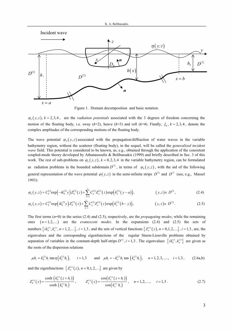
We consider the 2D problem concerning the hydrodynamic behavior of a floating body ( BD ) of arbitrary cross (yz) section in the coastal-marine environment, as illustrated in Fig. 1. The environment consists of a water layer bounded above by the free surface and below by a rigid bottom. It is assumed that the bottom surface exhibits an arbitrary one-dimensional variation, i.e. the bathymetry is characterised by parallel, straight bottom contours lying between two regions of constant but different depth, 1h h= (the deeper water region or region of incidence) and 3h h= (the shallower water region or region of transmission).

A Cartesian coordinate system { }, ,x y z

D

is introduced, with its origin at some point on the mean water level (in the variable bathymetry region), coinciding with the center of flotation of the floating body, and the z-axis pointing upwards. The liquid domain is decomposed in three parts ( )mD , 1, 2,3m = (see Fig. 1), defined as follows: is the subdomain characterized by ( )1D y a< where the depth is constant and equal to , and 1h ( )3D is

the subdomain characterized by where the depth is constant and equal to h . Also, y b> 3( )2D is the variable

bathymetry subdomain ( ) containing the floating and/or immersed body(ies). The depth function characterizing this environment is assumed to be smooth and has the following form

a y b< <

(2.1) ( ) ( )1

2

3

,,,

h y ah y h y a y b

h y b

≤= < ≥

<

)

The liquid is assumed homogeneous, inviscid and incompressible. The wave field in the region D is excited by a harmonic incident wave, with direction of propagation normal to the depth-contours. Thus, the fluid motion is described by the 2D wave potential ( , ;y z tΦ . The latter, under the assumptions that the free-surface elevation and the wave velocities are small, satisfies the linearised water wave equations. See, e.g., Wehausen & Laitone (1960) or Mei (1983). Then, the wave field is time harmonic

( ) ( ) ( ), ; Re , ; exp2igHy z t y z i tϕ µ ωω

Φ = − ⋅ −

, (2.2a)

where H is the incident wave height, g is the acceleration due to gravity, 2 / gµ ω= is the frequency

parameter, and 1i = − . The free surface elevation is obtained in terms of the wave potential on the free surface as follows

( ) ( ), 01;y z

y tg t

η∂Φ =

= −∂

. (2.2b)

The function ( , ;y z )ϕ ϕ=

( ),

µ , appearing in Eqs. (2.2), is the normalised potential in the frequency domain,

simply written as x zϕ . Using standard floating-body hydrodynamics theory (Wehausen, 1971), the potential

( , )y zϕ can be decomposed as follows

( ) ( ) ( ) ( )4

02

, , ,2P

k

i Hy z y z y z y zωϕ ϕ ϕ ξ ϕ=

= − +

∑ ,k k

)

, (2.3)

where ( ,P y zϕ denotes the propagation/diffraction wave potential, corresponding to the solution of the water-

wave problem in the variable bathymetry region in the absence of the scatterer BD . Moreover, (0 , )y zϕ is the diffraction wave potential in the non-uniform strip D due to the presence of the fixed body BD , and

2

K. A. Belibassakis

3

4

Incident wave D

Figure 1. Domain decomposition and basic notation.

1h

3h

y

z

( )2D

( )3D( )h x

n

x b=

x

( )y;tη

BD( )1

x a=

n

( ), , 2,3,4k y z kϕ = , are the radiation potentials associated with the 3 degrees of freedom concerning the

motion of the floating body, i.e. sway (k=2), heave (k=3) and roll (k=4). Finally, , 2,3,k kξ = , denote the complex amplitudes of the corresponding motions of the floating body. The wave potential ( ,P )y zϕ associated with the propagation/diffraction of water waves in the variable bathymetry region, without the scatterer (floating body), in the sequel, will be called the generalized incident wave field. This potential is considered to be known, as, e.g., obtained through the application of the consistent coupled-mode theory developed by Athanassoulis & Belibassakis (1999) and briefly described in Sec. 3 of this work. The rest of sub-problems on in the variable bathymetry region, can be formulated

as radiation problems in the bounded subdomain

( ), , 0, 2,3,4k y z kϕ =( )2D , in terms of ( ),P y zϕ , with the aid of the following

general representation of the wave potential ( ),y zϕ in the semi-infinite strips ( )1D and ( )3D (see, e.g., Massel 1993):

( ) ( ) ( )( ) ( ) ( ) ( ) ( ) ( ) ( ) ((1 1 1 1 1 10 0 0

1

, exp expk n nn

y z C ik y Z z C Z z k y aϕ∞

=

= − + −∑ ))n , ( ) ( )1,y z D∈ , (2.4)

( ) ( ) ( )( ) ( ) ( ) ( ) ( ) ( ) ( ) ( )(3 3 3 3 3 30 0 0

1, exp expk n n

ny z C ik y Z z C Z z k b yϕ

∞

=

= +∑ ) ,n − ( ) ( )3,y z D∈ . (2.5)

The first terms (n=0) in the series (2.4) and (2.5), respectively, are the propagating modes, while the remaining ones are the evanescent modes. In the expansions (2.4) and (2.5) the sets of

numbers , and the sets of vertical functions

( 1,2,n = …

{ ( ) ( )0 , ,i i

nik k

)} 3=1, 2, , 1,n i= … ( ){ }( ) , 0,1, 2, , 1,i

nZ z n i= …

{ }( ) ( )0 ,i i

nik k

3=

3

, are, the

eigenvalues and the corresponding eigenfunctions of the regular Sturm-Liouville problems obtained by separation of variables in the constant-depth half-strips . The eigenvalues are given as the roots of the dispersion relations

( ) , 1,iD i =

and ( ) ( )( )0 0tan , 1,3i i

i i ih k h k h iµ η= = ( ) ( )( )tan , 1, 2,3,....., 1,3i ii n i n ih k h k h n iµ = − = = , (2.6a,b)

and the eigenfunctions are given by ( ){ }( ) , 0,1, 2,inZ z n = …

( )( )( )

( )( )0( )

0 ( )0

cosh

cosh

iii

ii

k z hZ z

k h

+= , ( )

( )( )( )( )

( )( )

cos

cos

in ii

n in i

k z hZ z

k h

+= , 1, 2, , 1,3n i= =… . (2.7)

K. A. Belibassakis The completeness of the expansions (2.4) and (2.5) follows by the standard theory of regular eigenvalue problems; see, e.g., Coddington and Levinson, (1955, Section 7.4). On the basis of these representations the hydrodynamic problems concerning the diffraction and radiation potentials ( ( ), , 0, 2,3,4k y z kϕ = ) can be all formulated as transmission problems, satisfying the following systems of equations, boundary and matching conditions:

2 0,kϕ∇ = ( ) ( )2,y z D∈ (2.8a)

0kkn

∂ϕµϕ

∂− = , ( ) (2), Fy z D∂∈ , 0k

n∂ϕ∂

= , ( ) (2),y z D∂ Π∈ , kkg

n∂ϕ∂

= , ( ), By z D∂∈ , (2.8b,c,d)

[ ]12 0kkn

∂ϕϕ

∂− =T , ( ) (12), Iy z D∂∈ , [ ]23 0k

kn∂ϕ

ϕ∂

− =T , ( ) (23), Iy z D∂∈ , (2.8e,f,g,h)

where is the Laplacian on the vertical (yz) plane, 2 2 2 2/ /y∇ = ∂ ∂ + ∂ ∂ 2z (2)

FD∂ and denote the free-

surface and bottom parts of the domain

(2)D∂ Π

( )2D , BD∂ denotes the (solid) boundary of the floating body, and , are the vertical interfaces located at x=a and x=b (respectively), separating the three-

subdomains , . The latter are also shown by using vertical dashed lines in Fig. 1. Moreover, in Eqs.

(2.8) denotes the unit normal vector to the boundary , directed to its exterior. The

operators

(12)ID∂

(23)ID∂

( )iD 1, 2,3i =

( )0, ,y zn n=n

[

(2)D∂

]12 kϕT [and ]23 kϕT are appropriate Dirichlet-to-Neumann (DtN) maps, see, e.g. Givoli (1991),

ensuring the complete matching of the wave fields ( ), , 0,2,3k y z kϕ = , 4 , on the vertical interfaces ,

, respectively. These operators are constructed exploiting the completeness properties of the vertical

bases , i=1,2, as follows:

(12)ID∂

(23)ID∂

( ){ ( ) , 0,1, 2,inZ z n = …}

[ ] ( ) ( ) ( ) ( ) ( ) ( ) ( ) ( ) ( ) ( ) ( ) ( )1 1

0 01 1 1 1 1 1

12 0 0 0 0 01

, ,k k n knz h z h

ik Z z y a z Z z dz k Z z y a z Z z dϕ ϕ ϕ==− =−

= = + =∑∫ ∫T z , (2.9)

[ ] ( ) ( ) ( ) ( ) ( ) ( ) ( ) ( ) ( ) ( ) ( ) ( )1 3

0 03 3 3 3 3 3

23 0 0 0 0 01

, ,k k n knz h z h

ik Z z y b z Z z dz k Z z y b z Z z dzϕ ϕ ϕ==− =−

= = + =∑∫ ∫T . (2.10)

Finally, the boundary data kg , , appearing in the right-hand side of Eq. (2.8d), are defined on the wetted body surface

0, 2,3, 4k =

BD∂ by the normal derivative of the generalized incident field, 0 /Pg nϕ= −∂ ∂ , and by the components of the generalized normal vector on the body boundary, 2 yg n= , 3 zg n= , 4 z yg yn zn= − .

3. CALCULATION OF THE GENERALISED INCIDENT WAVE-FIELD The wave potential ( ,P )y zϕ associated with the propagation/diffraction of water waves in the variable bathymetry region, without the presence of the scatterer (floating body), can be very conveniently treated by means of the consistent coupled-mode theory (Athanassoulis & Belibassakis, 1999). This theory is based on the following enhanced local-mode representation of the generalised incident field (in the absence of the scatterers):

. (3.1) ( ) ( ) ( ) ( ) ( ) ( ) ( )1 1 0 01

, ; ;P n nn

y z y Z z y y Z z y y Z z yϕ ϕ ϕ ϕ∞

− −=

= + +∑ ;

In Eq. (3.1) the term ( ) (0 0 ;y Z z yϕ

( ) ( ); ,n ny Z z y) denotes the propagating mode of the generalised incident field. The

remaining terms , are the evanescent modes, and the additional term

is a correction term called the sloping-bottom mode, which properly accounts for the satisfaction of the Neumann bottom boundary condition on the non-horizontal parts of the bottom. The

1,2,nϕ = …

( ) ( )1 1 ;y Z z yϕ− −

4

K. A. Belibassakis

5

)function ( ;nZ z y represents the vertical structure of the -th mode. The function n ( )n yϕn

describes the horizontal pattern of the -th mode and is called the complex amplitude of the -th mode. The functions

n

( );nZ z y , , appearing in Eq. (3.1) are obtained as the eigenfunctions of local vertical Sturm-Liouville problems, and are given by

0,1,n = 2...

( )( ) ( )( )( ) ( )( ) ( )

( ) ( )( )( ) ( )( )

00

0

cosh cos; , ;

cosh cosn

nn

k y z h y k y z h yZ z y Z z y n

k y h y k y h y

+ + = = …, 1,2,=

}

, (3.2a)

where the eigenvalues { are obtained as the roots of the local dispersion relation ( ) ( )0 , nik y k y

( ) ( ) ( ) ( ) ( ) tanh y k y h y k y h yµ = − , a x b≤ ≤ . (3.2b) A specific convenient form of the function ( )1 ;Z z y− is given by

( ) ( ) ( ) ( )

3 2

1 ; z zZ z y h yh y h y−

= +

, (3.2c)

and all numerical results presented in this work are based on this choice for ( )1 ;Z z y− . However, other choices are also possible; see Athanassoulis & Belibassakis (1999, Sec.4). By following exactly the same procedure as in the latter work, the coupled-mode system of horizontal equations for the amplitudes of the generalised incident wave field is obtained:

, (3.3) ( ) ( ) ( ) ( ) ( ) ( )1

0, , 1,0,1,....mn n mn n mn nn

a y y b y y c y y a y b mϕ ϕ ϕ∞

=−

′′ ′+ + = < < = −∑ where a prime denotes differentiation with respect to y. The coefficients of the system (3.3) are dependent on y through

, ,mn mn mna b c

( )h y and can be found in Table 1 of Athanassoulis & Belibassakis (1999). The coupled-mode system (3.3) is supplemented by the following boundary conditions (see also Massel, 1993)

( ) ( )1 1 0a aϕ ϕ− −′= = , ( ) ( )1 1 0b bϕ ϕ− −′= = , (3.4a,a’)

( ) ( ) ( ) ( ) ( )(1 10 0 0 0 02 expa ik a i k i k aϕ ϕ′ + = )1 , ( ) ( )(1) 0, 1,2,..n n na k a nϕ ϕ′ − = = , (3.4b,b’)

( ) ( )(3)

0 0 0 0b ik bϕ ϕ′ − = , ( ) ( )(3) 0, 1,2,3,n n nb k b nϕ ϕ′ + = = … . (3.4c,c’)

In the above equations { are the eigenvalues( ) ( )1 10 , nik k } ( ) ( ){ }0 , n y a

ik y k y=

, which remain the same all over the

region , and { are the eigenvalues(1)D ( )0ik ( )}3 3, nk ( ) ( ){ }0 , n y b

y k yik=

, which remain the same all over the

region . On the basis of the solution of the coupled-mode system, the reflection and transmission coefficients (

(3)D,R TA A ) of the waves propagating and diffracted in the variable bathymetry region without the presence of the

floating body can be calculated as follows ( ) ( )( ) ((1) (1)

0 0exp expR )0A a i k a i kϕ= − a , ( ) ( )(3)0 expT 0A b i kϕ= − b , (3.5)

An important feature of the solution of the generalized incident problem by means of the enhanced representation (3.1), is that it exhibits an improved rate of decay of the modal amplitudes ( )n yϕ

( ),

of the

order O n . Thus, only a few number of modes suffice to obtain a convergent solution to( 4− ) P y zϕ , even for bottom slopes of the order of 1:1, or higher. More details can be found in Athanassoulis & Belibassakis (1999).

K. A. Belibassakis 4. THE BOUNDARY INTEGRAL EQUATION FOR THE DIFFRACTION-RADIATION PROBLEMS The problems on , Eqs. (2.8), will be treated by means of equivalent boundary integral equation formulations, based on the single layer potential (see, e.g., Wehausen, 1974). Accordingly, the following integral representations are introduced for

( ), , 0, 2,3, 4k x z kϕ =

( ), , 0, 2,3, 4k x z kϕ = , in ( )2D :

( ) ( ) ( ) ( )( )

( ) ( ) ( )

2

2, , ,2k k

D

G d D , y z Dϕ σ∂

′ ′ ′ ′= ∈∫r r r r r r r = ∈∂ 0,2,3, 4k, = . (4.1)

where ( )ln

,2

-G

π′

′ =r r

r r is the Green’s function of the Laplace equation in 2D, and denotes the

differential element along the boundary

( )d ′r

( )2D∂ ; see, e.g., Kress (1989), Katz-Plotkin (1991). Based on the properties of the single-layer distributions, the corresponding normal derivatives of the potentials

, on the boundary ( ), , 0, 2,3, 4k =k x zϕ ( )2D∂ are given by (Kress, 1989):

( ) ( ) ( ) ( ) ( )( )

( ) ( ) ( )

2

2,,

22k k

k

D

Gd D , y z

n nϕ σ

σ∂

′∂ ∂′ ′ ′= − + ∈∂ ∈∂

∂ ∂∫r r r r

r r r r = , D . (4.2)

Using Eqs. (4.1) and (4.2) in Eqs (2.8) we obtain, for each potential ( ), , 0, 2,3, 4k x z kϕ = , a boundary integral

equation with support on ( )2D∂ for the determination of the corresponding source distribution ( ) ( ), 2k Dσ ∈∂r r .

Then, all quantities of interest associated with these wave potentials (or their superposition, Eq. 2.3), can be calculated by means of Eq. (4.1) and similar ones expressing their spatial derivatives (flow velocity field), in the flow domain.

5. EQUATIONS OF MOTION

On the basis of the calculated potential ( ) ( )0, ,P x z x zϕ ϕ+

kF k,

4the Froude-Krylov and the diffraction-induced

hydrodynamic forces and moment on the floating body , 2,3,= can be calculated. Moreover, using the radiation potentials , the hydrodynamic coefficients (the symmetric matrices of added masses and damping coefficients ) can be calculated, permitting us to formulate and solve the equations of motion of the floating body in the variable bathymetry region. The general form of equations of motion concerning the floating body is as follows:

( ), , 2,3,k x z kϕ =

klb4

kla

( )( ) ( )2 2

22 22 2 24 24 4 2m a i b a i b Fω ω ξ ω ω ξ− + − − + = , (5.1a)

( )( 233 33 3 3m a i b gB Fω ω ρ ξ− + − + =) , (5.1b)

( ) ( )(2 242 42 2 2 44 44 4 4a i b m a i b mgGM Fω ω ξ ω ω ξ− − + − + − + =) , (5.1c)

where B is the breadth of the floating body and GM denotes its metacentric height. The above equations can also be modified to include other external forces, as e.g., mooring forces or spring terms; see, e.g. Drimer et al (1992, Sec. 3.5). Details about the definitions of the hydrodynamic forces and coefficients, as well as the system of equations of motion, Eqs. (5.1), can be found in Wehausen (1971) or in any other ship hydrodynamics textbook (see, e.g, Lewis, 1989).

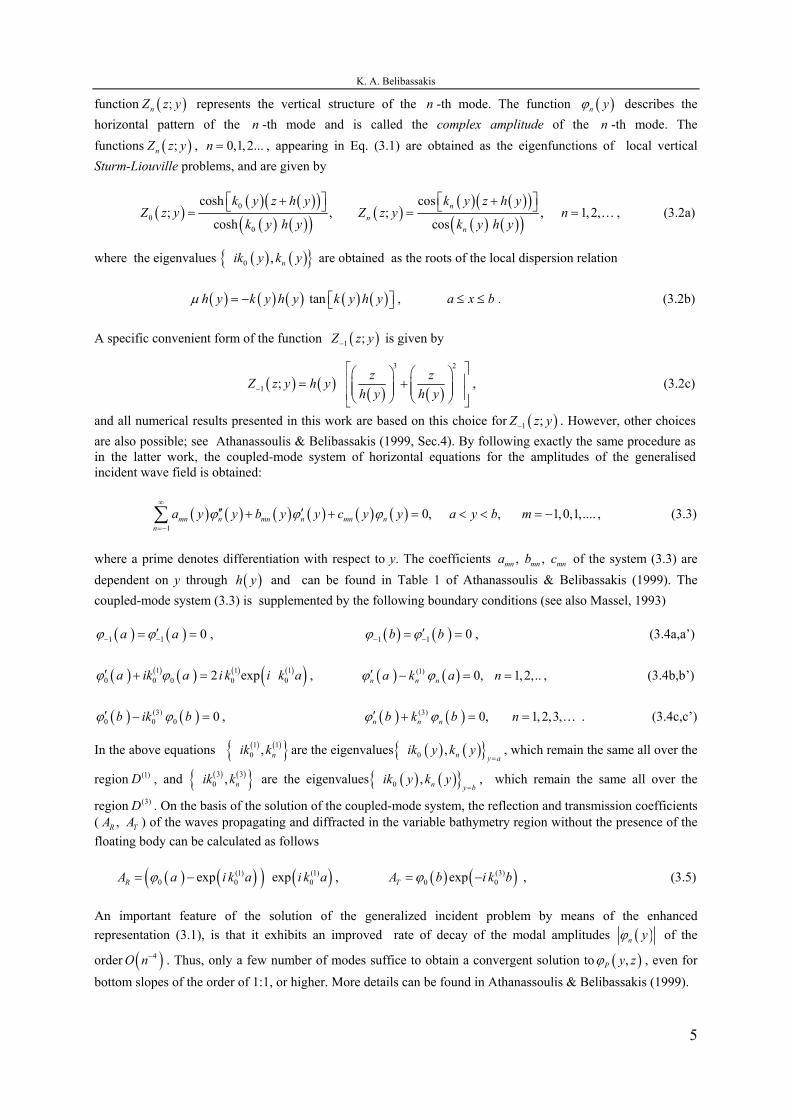
6. NUMERICAL RESULTS AND CONCLUSIONS To illustrate the effects of bottom slope on the hydrodynamic characteristics of floating bodies in variable bathymetry regions, we consider, as an example, the case of a floating pontoon, i.e. a floating body of rectangular cross section, with nondimensional breadth B/h=1.5, and draft T/h=0.5, where h denotes the (mean) depth below the centerline of the floating body. See Fig. 2(a). The center of gravity has been selected to coincide with the center of flotation (KG=T) and thus, the metacentric height of this structure is GM/h=0.625.

6

K. A. Belibassakis Numerical results are presented in Figs. 2 and 3 concerning the hydrodynamic behavior of this floating structure in constant depth and over two linear shoals characterized by (constant) bottom slopes 12.5% and 25%, respectively. More specifically, in Fig. 2 the effect of bottom slope on the hydrodynamic forces, the added mass and the damping coefficients is examined. In Fig.3(a), the same effect is illustrated concerning transmission coefficient of the rectangular pontoon, considered to be freely floating and fixed. In the rest subplots of Fig. 3, the effect of bottom slope on the motions of the freely floating body is presented. In this case, the response amplitude operators (RAOs) of the floating pontoon in sway, heave and roll motion are presented, as calculated by the present method, over flat and sloping seabeds. All the above results are parametrically plotted vs. the non-dimansional wavelength λ/h, ranging from deep ( / h 0λ → ) to shallow ( / hλ →∞ ) wave conditions. From the results presented, we can clearly observe that the effects of bottom slope (and, in general, of the bottom variations) on the hydrodynamic characteristics of the floating bodies can be important, especially in the case of intermediate and shallow water conditions ( / h 7λ > ) . In this case, the present method can serve as a useful tool for the design and performance evaluation of floating structures and ships operating in nearshore and coastal waters.

Acknowledgements: The present work has been financially supported by the “ARCHIMEDES”-TEI of Athens program, funded in the framework of Operational Programme for Education and Initial Vocational Training (EPEAEK), which is coordinated by the Greek Ministry of National Education and the European Union.

REFERENCES

[1] Athanassoulis G.A., Belibassakis, K.A. (1999), “A consistent coupled-mode theory for the propagation of small-amplitude water waves over variable bathymetry regions” J. Fluid Mech. Vol. 389, 275-301.

[2] Belibassakis, K.A., Athanassoulis G.A., G.A. & Gerostathis, T.P. (2001), “A coupled-mode model for the refraction-diffraction of linear waves over steep three-dimensional bathymetry” Applied Ocean Research Vol. 23, 319-336.

2F

3F

4F

22a

22b

33a

33b

24a

24b

44a

441 0b

1 2 .5%25%

0 %fla t

( )a

( )f

( )e

( )b

( )d

( )c

/ hλ

Figure 2. (a) Geometrical configuration, (b) Hydrodynamic forces , 2,3,kF k 4= , and (c,d,e,f) coefficients vs. the non dimensional wavelength λ/h (where 02 / kλ π= , as obtained using the linearised dispersion relation, Eq. 2.6a), in the case of a floating body of rectangular cross section B/h=1.5, T/h=0.5. The three bottom profiles considered are (i) flat bottom (solid lines), (ii) sloping sea-bed 12.5% (dashed-dotted lines), and (iii) sloping sea-bed 25% (dashed lines). Added mass and damping coefficients of (c) the sway motion, (d) the heave motion, (e) the coupled sway-roll, and (f) the roll motion. The scaling used for the hydrodynamic forces is:

24 42 / , 2,3, 2 /k kF F ghH k F F gh Hρ= = =

324 24 / ,a a hρ= 4

44 44 /a a h

ρ , for the added-mass coefficients: 2/ , , 2,3kl kla a h k lρ= = ,

ρ= , and for the damping coefficients 2/ / , , 2,kl h h g k lρ= = 3,klb b 3

24 24 / / ,b b h h gρ= 444 44 / /b b h h gρ= , where ρ is the fluid (water) density and h is the (mean) water depth.

7

K. A. Belibassakis

free

fixed

( )a

( )c

( )b

( )d

/ hλ

Roll

Figure 3. (a) Transmission coefficient of fixed and freely floating body of rectangular cross section B/h=1.5, T/h=0.5, in flat sea-bed (solid line), and sloping seabeds 12.5% (dashed-dotted line) and 25% (dashed line) (b,c) Floating body RAO in sway and heave motion ( 2 / ),respectively, and (d) Floating body RAO in

roll motion (

, 2,k H kξ = 3

42 / kHξ ), vs. the non dimensional wave length λ/h (where 02 / kλ π= , is the wavelength of the incident wave, as obtained using the linearised dispersion relation, Eq. 2.6a). [3] Coddington, E.A., Levinson N. (1955), Theory of Ordinary Differential Equations. McGraw Hill, New

York. [4] Eatock Taylor, R., Ohkusu, M. (Eds., 2000), Journal of Fluids and Structures. Special issue, Vol. 14, No. 7. [5] Ertekin C.R, Kim, J.W., Yoshida K. & Mansour A.E. (Eds. 2000, 2001), Marine Structures. Special issues,

Vol. 13 No. 4,5 and Vol. 14 No. 1,2. [6] Drimer, N., Agnon, Y., Stiassnie, M. (1992), “A simplified analytical model for a floating breakwater in

water of finite depth”, Applied Ocean Research, Vol. 14, pp. 33-41. [7] Drobyshevski, Y. (2004), “Hydrodynamic coefficients of a two-dimensional, truncated rectangular floating

structure in shallow water”, Ocean Engng. [8] Givoli, D. (1991) “Non-reflecting boundary conditions”, J. Comp. Physics Vol. 94, 1-29. [9] Katz, J., Plotkin, A. (1991) Low speed aerodynamics, McGraw Hill. [10] Kress, R., (1989), Linear integral equations, Springer Verlag, Berlin. [11] Lewis, E.V. (Ed., 1989), Principles of Naval Architecture, Vol. III, SNAME, NJ [12] Massel, S. (1993), “Extended refraction-diffraction equations for surface waves”. Coastal Engng Vol.19,

97-126. [13] Mei, C.C. (1983), The applied dynamics of ocean surface waves. Second Edition 1996, World Scientific. [14] Ohyama, T., Tsuchida, M. (1997), “Expanded mild-slope equations for the analysis of wave-induced ship

motion in a harbor”, Coastal Engng, Vol. 30, pp.77-103 [15] Sawaragi, T. (1995) Coastal Engineering - Waves, Beaches, Wave-Structure Interactions, Elsevier. [16] Takagi, K., Naito, S. and Hirota, K. (1993) “Hydrodynamic forces acting on a floating body in a harbour of

arbitrary geometry”, 3rd Intern Offshore and Polar Eng, Conference (ISOPE) Vol. 3, pp. 192-199. [17] Wehausen, J.V. (1971), “The motion of floating bodies, Ann. Review of Fluid Mechanics”, Vol. 3, 237-268 [18] Wehausen, J.V. (1974), Methods for boundary-value problems in free-surface flows, David Taylor Naval

Ship Research and Development Center DTNSRDC Rep. 4622, Bethesda, Md. [19] Wehausen, J. and Laitone, E. (1960) Surface Waves. Encyclopedia of Physics, Fluid Dynamics III 9,

Springer-Verlag. [20] Williams, K.J. (1988), “The boundary integral equation for the solution of wave-obstacle interaction”, Int.

Journal for Numerical Methods in Fluids, Vol. 8, pp. 227-242. [21] Williams, A.N., Lee, H.S. and Huang, Z. (2000), “Floating pontoon breakwaters”, Ocean Engineering Vol.

27, pp. 221–240.

8