hyp oth esis testi ng stat 305: chapter 6 - part ii
TRANSCRIPT
STAT 305: Chapter 6 - Part IISTAT 305: Chapter 6 - Part II
Hypothesis TestingHypothesis Testing
Amin ShiraziAmin Shirazi
Course page:Course page:ashirazist.github.io/stat305.github.ioashirazist.github.io/stat305.github.io
1 / 901 / 90

Hypothesis TestingHypothesis TestingDeciding What's True (Even If We're Just Guessing)Deciding What's True (Even If We're Just Guessing)
2 / 902 / 90

Let's Play A GameLet's Play A GameA "Friendly" Introduction to Hypothesis TestsA "Friendly" Introduction to Hypothesis Tests
3 / 903 / 90

My Game
The RulesLet's Play A GameThe semester is getting a little intense! You are a livinLet'sbreak the tension with a friendly game.
Here are the rules:
I have a new deck of cards. 52 Cards, 26 with Suits thatare Red, 26 with Suits that are BlackYou draw a red-suited card, you give me a dollarYou draw a black-suited card, I give you two dollars
Quick Questions
What is the expected number of dollars you will winplaying this game?
Would you play this game?
4 / 90

Are We Forgetting Something?Are We Forgetting Something?
5 / 905 / 90

My Game
The Rules
TheAssumptions
Be Careful About Your Assumptions
Pause for a minute and think about what you areassuming is true when you play this game. For instance,
You assume I'm going to shuffle the cards fairlyYou assume there are 52 cards in the deckYou assume the deck has 26 red-suited cards in itYou assume the deck has a red-suited card in it
How can we make sure the assumptions are safe??
Shuffling assumption: watch me shuffle, make sureI'm not doing magic tricks, etc52 Cards assumption: count the cardsRed-suit assumption: Count the number of red cards
Whew! We can actually make sure all of our assumptionsare good!
6 / 90

One ProblemOne ProblemI Refuse to Show You The CardsI Refuse to Show You The Cards
7 / 907 / 90

Do You Trust Me?Do You Trust Me?
8 / 908 / 90

My Game
The Rules
TheAssumptions
Our Assumptions
I'm not going to show you all the cards. In other words, Irefuse to show you the population of possible outcomes.This is justified: we are in a statistics course after all.
So, let's start with our unverifiable assumption: Is it safe toassume that this is a fair game. Why would we make thisassumption?
You trust that I'm (basically) an honest person(assumption of decency)You trust that I'm getting paid enough that I wouldn'trisk cheating students out of money (assumption ofpracticality)You saw the deck was new (manufacturer trustassumption)You want it to be an fair game because you would winlots of money if it was (assumption in self-interest)
9 / 90

My Game
The Rules
TheAssumptions
Our Assumptions
In statistical terminology, we wrap all these assumptionsup into one assumption: our "null hypothesis" is that thegame is not rigged - that the probability of you winning is0.5
Null Hypothesis The assumptions we are operate under innormal circumstances (i.e., what we believe istrue). We wrap these assumptions up into astatistical/mathematical statement, but we willaccept them unless we have reason to doubtthem. We use the notation H0 to refer to thenull hypothesis.
In this case, we could say that the probability of winning isp and that would make our null hypothesis
H0 : p = 0.5
10 / 90

My Game
The Rules
TheAssumptions
Our Assumptions
Of course our assumptions could be wrong. We call theother assumptions our "alternative hypothesis":
Alternative Hypothesis The conditions that we do require proof toaccept. We would have to change our beliefsbased on evidence. We use the notation HA (orsometimes, H1) to refer to the alternative
hypothesis.
In this case, we could say that our alternative to believingthe game is "fair" is to believe the game is not fair, or thatthe probability of winning is not 0.5. We write:
HA : p ≠ 0.5
11 / 90

A CompromiseA CompromiseI Won't Show You All The CardsI Won't Show You All The Cards
But I Will Let You Test The GameBut I Will Let You Test The Game
12 / 9012 / 90

My Game
The Rules
TheAssumptions
The Test
Testing the Game
The test of whether or not the game is worth playing canbe defined in term of whether or not our assumptions aretrue. In other words, we are going to test whether our nullhypothesis is correct:
Hypothesis Tests A hypothesis test is a way of checking if theoutcomes of a random experiment arestatistically unusual based on our assumptions.If we see really unusual results, then we havestatistically significant evidence that allowsus to reject our null hypothesis. If ourassumptions lead to results that are notunusual, then we fail to reject our nullhypothesis.
13 / 90

My Game
The Rules
TheAssumptions
The Test
Testing the Game
So how can we test the game? What if we tried a singleround of the game?
What are the probabilities of the outcome of a singlegame?If we draw a single card do we have enough evidencethat the game is fair?Do we have enough evidence that the game is rigged?
Based on a single round of the game, both of the possibeloutcomes are pretty normal - that's not good enough.
If we draw a losing card, then we might be inclined to callthe game unfair - even though a losing card is prettycommon for a single round of the game
If we draw a winning card, then we might be inclined tocall the game fair - even though a winning card may becommon even when the game is not fair!
We can make lots of mistakes!!
14 / 90
My Game
The Rules
TheAssumptions
The Test
The Errors
The Mistakes We Might Make
We could of course be wrong: For instance, we could, justby random chance, see outcomes that are unusual for theassumptions we make and reject the assumptions even if(in reality they are true). This is called a "Type I Error"
Type I Error When the results of a hypothesis test lead us toreject the assumptions, while the assumptionsare actually true, we have committed a Type IError.
15 / 90

My Game
The Rules
TheAssumptions
The Test
The Errors
The Mistakes We Might Make
A common example of this is found in criminal court:
We assume that a individual accused of a crime isinnocent (our assumption)After examinig the evidence, we conclude that it isthere is no reasonable doubt the person is notinnocent (in other words, we reject the assumptionbecause it is very unlikely to be true based on ourevidence).If the person truly is innocent, then we havecommitted a Type I error (rejecting assumptions thatwere true).
16 / 90
My Game
The Rules
TheAssumptions
The Test
The Errors
The Mistakes We Might Make
We could also make a different error: we could choose notto reject the assumptions when in reality the assumptionsare wrong.
Type II Error When the results of a hypothesis test lead us tofail to reject the assumptions, while theassumptions are actually false, we havecommitted a Type II Error.
17 / 90

My Game
The Rules
TheAssumptions
The Test
The Errors
The Mistakes We Might Make
Again, if we consider the example of criminal court:
We assume that a individual accused of a crime isinnocent (our assumption)After examinig the evidence, we conclude that it isthere is not evidence beyond a reasonable doubt theperson is not innocent (in other words, the evidence isnot enough to reject our assumption because it is stillreasonable to doubt the accused's guilt).If the person truly is not innocent, then we havecommitted a Type II error (failing to rejectassumptions that were false).
In general, we want to make sure that a Type I error isunlikely. To take the example of court again,
We commit a Type II error: a guilty person goes freeWe commit a Type I error: an innocent person goes tojail; the guiilty person is still free
18 / 90

My Game
The Rules
TheAssumptions
The Test
The Errors
The Mistakes We Might Make
Let's go back to my game: We assume I am an honestperson (i.e., we assume that the probability of winning asingle game is p = 0.5)Type I Error: Rejecting True Assumptions
We gather evidenceLooking at our evidence, we decide that the game wasnot fair even though it was.Fallout: you slander me, you disparge me, we have afight, BOOOM.
Type II Error: Failing to Reject False Assumptions
We gather evidenceLooking at our evidence, we decide that the game wasfair even though it was not.Fallout: you play the game and lose some money.
Ideally, we won't make either error. However, we can onlybase our decision of our evidence we can gather - the truthis out of our grasp!
19 / 90
My Game
The Rules
TheAssumptions
The Test
The Errors
The Evidence
Gathering Statistical Evidence
Okay, so we don't want to make either error - that meanswe need good evidence.
Like we talked about before, even if the game is fair onetest round of the game would not be enough to make agood decision since drawing a red-suited card anddrawing a black-suited card are both pretty normal for asingle round of the game.
But what if we played the game 10 times in a row? After 10rounds, do you think we would have enough evidence tomake a decision about our assumption?
20 / 90

My Game
The Rules
TheAssumptions
The Test
The Errors
The Evidence
p-value
p-value
If we assume the null hypothesis, then we can make someassumptions about what results are likely and whatresults are unlikely. We describe the likelihood of theresults that we actually get using a p-value
p-value After gathering evidence (aka, data) we candetermine the probability that we would havegotten the evidence we did if our assumptionswere true. That probabiliity is called the p-value. If the p-value is really, really small thatmeans that the assumptions we started withare pretty unlikely and we reject ourassumptions. If the p-values is not small, thenthe evidence collected (aka, the data) is prettynormal for our assumptions and we fail toreject our assumptions.
21 / 90

My Game
The Rules
TheAssumptions
The Test
The Errors
The Evidence
p-value
p-value
In other words, we collect evidence and determine a wayto measure the whether or not our data was unusual if ourassumptions are true.
If we have a very, very low chance of
seeing both our results andhaving true assumptions then we reject theassumptions
Going along with the terminology we have introduced, ifwe have a small p-value then we reject our nullhypothesis.
22 / 90

My Game
The Rules
TheAssumptions
The Test
The Errors
The Evidence
p-value
Gathering Statistical Evidence
In this game, if we assume that the game is fair, we have
two outcomes: success (winning) and failure (losing)a constant chance of a successful outcome (p = 0.5),assuming the game is fair)independent rounds of the game (assuming fairshuffle, which we can check)
In other words, if we test the game 10 times we can modelthe number of successful outcomes as binomial: For X =the total number of wins,
P(X = x) =10!x !
(10 − x) !(0.5)x(1 − 0.5)10 − x
This gives us a way of getting our p-value
23 / 90

Let's Test the GameLet's Test the Game
24 / 9024 / 90

My Game
The Rules
TheAssumptions
The Test
The Errors
The Evidence
p-value
TheConclusion
Gathering Statistical Evidence
We played the game. Let's figure out whether our resultswere unusual or not.
Again, we assume the game is fair and have decided thatthe number of times we win will follow a binomialdistribution with probabiliity function
P(X = x) =10!x !
(10 − x) !(0.5)x(1 − 0.5)10 − x
Now we need to make a conclusion: do we accept or rejectour assumptions? What do we consider unusual? Is it fairto decide after we play?
25 / 90

My Game
The Rules
TheAssumptions
The Test
The Errors
The Evidence
p-value
TheConclusion
Summary
Sometimes we can know if something is true or not byexamining the truth directly, but not alwaysWhen we can't examine the truth, we need to testwhat we believe to be trueA statistical test is a tool for testing our assumptionsabout what we believe
We state our assumed belief (generally ourcurrent beliefs, or the ethical beliefs, or the beliefswe hope are true, ...)We come up with a way of collecting data thatcould validate or invalidate our assumptionWe measure how likely it was that we would havegathered the data we did if our assumptions werecorrectWe reject the assumptions if our data is veryunlikely we are our current beliefs
26 / 90

Now let's make everythingNow let's make everything
a little more formala little more formal
27 / 9027 / 90

Section 6.3Section 6.3
Hypothesis TestingHypothesis Testing
28 / 9028 / 90

HypothesisTesting Hypothesis testing
Last section illustrated how probability can enableconfidence interval estimation. We can also useprobability as a means to use data to quantitatively assessthe plausibility of a trial value of a parameter.
Statistical inference is using data from the sample todraw conclusions about the population.
1. Interval estimation (confidenceintervals): Estimates population parameters andspecifying the degree of precision of theestimate.
1. Hypothesis testing: Testing the validity of statements about thepopulation that are formed in terms ofparameters.
29 / 90

HypothesisTesting
Null
De�nition:
Statistical significance testing is the use of data in thequantitative assessment of the plausibility of some trialvalue for a parameter (or function of one or moreparameters).Significance (or hypothesis) testing begins with thespecification of a trial value (or hypothesis).
A null hypothesis is a statement of the form
Parameter = #
or
Function of parameters = #
for some # that forms the basis of investigation in asignificance test. A null hypothesis is usually formed toembody a status quo/"pre-data" view of the parameter. It isdenoted H0.
30 / 90

HypothesisTesting
Null
Alternative
De�nition:
An alternative hypothesis is a statement that stands inopposition to the null hypothesis. It specifies what formsof departure from the null hypothesis are of concern. Analternative hypothesis is denoted as Ha. It is of the form
Parameter ≠ #
or
Parameter > # or Parameter < #
Examples (testing the true mean value):
H0 : μ = # H0 : μ = # H0 : μ = #
Ha : μ ≠ # Ha : μ > # Ha : μ < #
Often, the alternative hypothesis is based on aninvestigator's suspicions and/or hopes about th true stateof affairs.
31 / 90

HypothesisTesting
Null
Alternative
The goal is to use the data to debunk the null hypothesis infavor of the alternative.
1. Assume H0.
2. Try to show that, under H0, the data are preposterous.
(using probability)
3. If the data are preposterous, reject H0 and conclude Ha.
The outcomes of a hypothesis test consists of:
32 / 90

HypothesisTesting
Null
Alternative
Probability of type I error
It is not possible to reduce both type I and type II erros atthe same time. The approach is then to fix one of them.
We then fix the probability of type I error and try tominimize the probability of type II error.
We define the probability of type I error to be α(the significance level)
33 / 90

HypothesisTesting
Null
Alternative
Example: [Fair coin]
Suppose we toss a coin n = 25 times, and the results aredenoted by X1, X2, …, X25. We use 1 to denote the result of ahead and 0 to denote the results of a tail. Then X1 ∼ Binomial(1, ρ) where ρ denotes the chance of getting
heads, so E(X1) = ρ, Var(X1) = ρ(1 − ρ). Given the result is yougot all heads, do you think the coin is fair?
Null hypothesis :H0 : the coin is fair or H0 : ρ = 0.5
Alternative hypothesis :Ha : ρ ≠ 0.5
If H0 was correct, then
P(results are all heads) = (1 /2)25 < 0.000001
I don't think this coin is fair (reject H0 in favorof Ha)
34 / 90

HypothesisTesting
Null
Alternative
In the real life, we may have data from many differentkinds of distributions! Thus we need a universalframework to deal with these kinds of problems.
We have n = 25 ≥ 25 iid trials ⇒ By CLT we know if H0 : ρ = 0.5( = E(X)) then
¯X − ρ
√ρ(1 − ρ) /n∼ N(0, 1)
We obsrved ¯X = 1, so
¯X − 0.5
√0.5(1 − 0.5) /25=
1 − 0.5
√0.5(1 − 0.5) /25= 5
Then the probability of seeing as wierd or wierder data is
P(Observing something wierd or wierder) =P(Z bigger than 5 or less than -5)
< 0.000001
35 / 90

HypothesisTesting
Null
Alternative
P-value
Signi�cance tests for a mean
Definition:A test statistic is the particular form of numerical datasummarization used in a significance test.
Definition:A reference (or null) distribution for a test statistic is theprobability distribution describing the test statistic,provided the null hypothesis is in fact true.
Definition:The observed level of significance or p-value in asignificance test is the probability that the referencedistribution assigns to the set of possible values of the teststatistic that are at least as extreme as the one actuallyobserved.
36 / 90

HypothesisTesting
Null
Alternative
P-value
Signi�cance tests for a mean
In the previous example, the test statistic was ¯X − ρ
√ρ(1 − ρ) /n∼ N(0, 1)
In the previous example, the null distribution was N(0, 1)
In the previous example, the p-value was < 0.000001
37 / 90

HypothesisTesting
Null
Alternative
P-value
Signi�cance tests for a mean
In other words:
Let K be the test statistics value based on the data
Say
H0 : μ = μ0
Ha : μ ≠ μ0
P(observing data as or more extreme as K) = P(Z < − K or Z > k)
is defined as the p-value
38 / 90

HypothesisTesting
Null
Alternative
P-value
Signi�cance tests for a mean
Based on our results from Section 6.2 of the notes, we candevelop hypothesis tests for the true mean value of adistribution in various situations, given an iid sample X1, …, Xn where H0 : μ = μ0.
Let K be the value of the test statistic, Z ∼ N(0, 1), and T ∼ tn− 1. Here is a table of p-values that you should use for
each set of conditions and choice of Ha.
39 / 90
HypothesisTesting
Null
Alternative
P-value
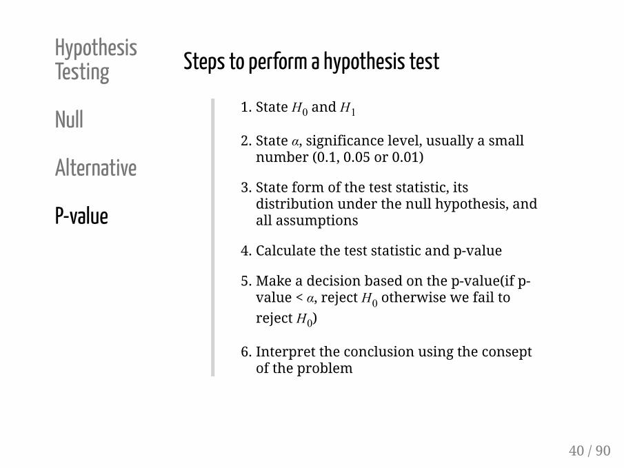
Steps to perform a hypothesis test
1. State H0 and H1
2. State α, significance level, usually a smallnumber (0.1, 0.05 or 0.01)
3. State form of the test statistic, itsdistribution under the null hypothesis, andall assumptions
4. Calculate the test statistic and p-value
5. Make a decision based on the p-value(if p-value < α, reject H0 otherwise we fail to
reject H0)
6. Interpret the conclusion using the conseptof the problem
40 / 90
HypothesisTesting
Null
Alternative
P-value
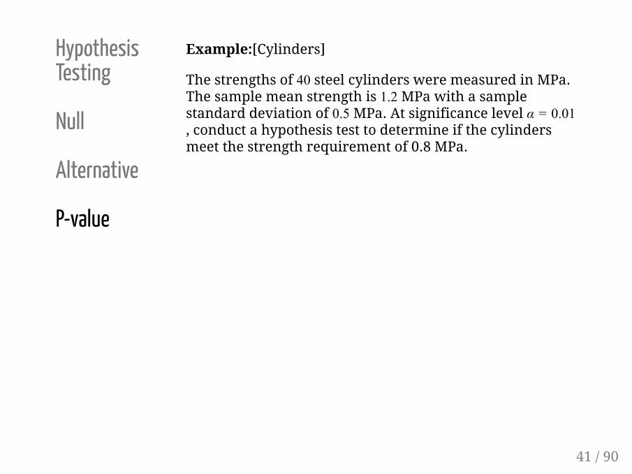
Example:[Cylinders]
The strengths of 40 steel cylinders were measured in MPa.The sample mean strength is 1.2 MPa with a samplestandard deviation of 0.5 MPa. At significance level α = 0.01, conduct a hypothesis test to determine if the cylindersmeet the strength requirement of 0.8 MPa.
41 / 90

HypothesisTesting
Null
Alternative
P-value
Example: [Concrete beams]
10 concrete beams were each measured for flexuralstrength (MPa). The data is as follows.
[1] 8.2 8.7 7.8 9.7 7.4 7.8 7.7 11.6 11.3 11.8
The sample mean was 9.2 MPa and the sample variancewas 3.0933 MPa. Conduct a hypothesis test to find out if theflexural strength is different from 9.0 MPa.
42 / 90

Hypothesis Testing Using Con�denceHypothesis Testing Using Con�denceIntervalInterval
43 / 9043 / 90

HypothesisTesting
Null
Alternative
P-value
Hypothesis testing using the CI
We can also use the 1 − α confidence interval to performhypothesis tests (instead of p-values). The confidenceinterval will contain μ0 when there is little to no evidenceagainst H0 and will not contain μ0 when there is strong
evidence against H0.
44 / 90

HypothesisTesting
Null
Alternative
P-value
CI method
Hypothesis testing using the CI
Steps to perform a hypothesis test using a confidenceinterval:
1. State H0 and H1
2. State α, significance level
3. State the form of 100 (1 − α) % CI along withall assumptions necessary. (use one-sidedCI for one-sided tests and two-sided CI fortwo sided tests)
4. Calculate the CI
5. Based on 100 (1 − α) % CI, either reject H0 (if
μ0 is not in the interval) or fail to reject (if μ0 is in the interval )
6. Interpret the conclusion in the content ofthe problem
45 / 90

HypothesisTesting
Null
Alternative
P-value
CI method
Example:[Breaking strength of wire, cont'd]
Suppose you are a manufacturer of constructionequipment. You make 0.0125 inch wire rope and need todetermine how much weight it can hold before breakingso that you can label it clearly. You have breakingstrengths, in kg, for 41 sample wires with sample meanbreaking strength 91.85 kg and sample standard deviation 17.6 kg. Using the appropriate 95% confidence interval,conduct a hypothesis test to find out if the true meanbreaking strength is above 85 kg.
Steps:
1- H0 : μ = 85 vs. H1 : μ > 85
2- α = 0.05
46 / 90

HypothesisTesting
Null
Alternative
P-value
CI method
Example:[Breaking strength of wire, cont'd]
3- One-sided test and we care about the lower
bound. So, we use (¯X − z1 −α
s
√n, + ∞).
4- From the example in previous set of slides,the CI is (87.3422, + ∞).
5- Since μ0 = 85 is not in the CI, we reject H0.
6- There is significant evidence to conclude thatthe true mean breaking strength of wire isgreater than the 85kg. Hence the requirementis met.
47 / 90
HypothesisTesting
Null
Alternative
P-value
CI method
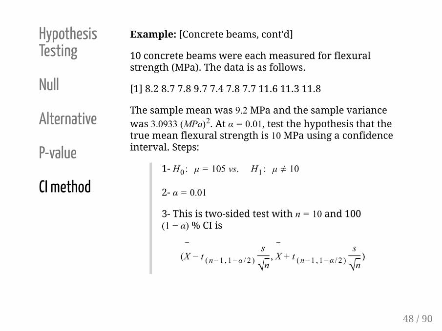
Example: [Concrete beams, cont'd]
10 concrete beams were each measured for flexuralstrength (MPa). The data is as follows.
[1] 8.2 8.7 7.8 9.7 7.4 7.8 7.7 11.6 11.3 11.8
The sample mean was 9.2 MPa and the sample variancewas 3.0933 (MPa)2. At α = 0.01, test the hypothesis that thetrue mean flexural strength is 10 MPa using a confidenceinterval. Steps:
1- H0 : μ = 105 vs. H1 : μ ≠ 10
2- α = 0.01
3- This is two-sided test with n = 10 and 100 (1 − α) % CI is
(¯X − t (n− 1 , 1 −α / 2 )
s
√n,
¯X + t (n− 1 , 1 −α / 2 )
s
√n)
48 / 90
HypothesisTesting
Null
Alternative
P-value
CI method
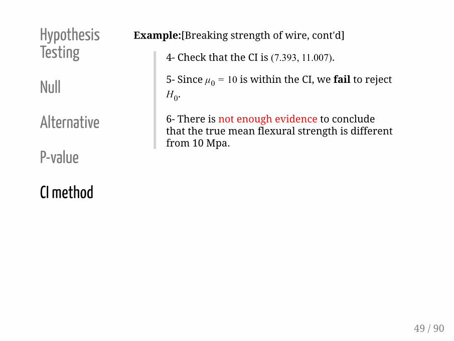
Example:[Breaking strength of wire, cont'd]
4- Check that the CI is (7.393, 11.007).
5- Since μ0 = 10 is within the CI, we fail to rejectH0.
6- There is not enough evidence to concludethat the true mean flexural strength is differentfrom 10 Mpa.
49 / 90
HypothesisTesting
Null
Alternative
P-value
CI method
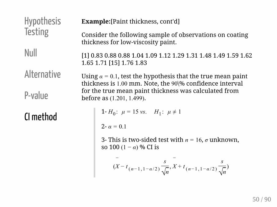
Example:[Paint thickness, cont'd]
Consider the following sample of observations on coatingthickness for low-viscosity paint.
[1] 0.83 0.88 0.88 1.04 1.09 1.12 1.29 1.31 1.48 1.49 1.59 1.621.65 1.71 [15] 1.76 1.83
Using α = 0.1, test the hypothesis that the true mean paintthickness is 1.00 mm. Note, the 90\% confidence intervalfor the true mean paint thickness was calculated frombefore as (1.201, 1.499).
1- H0 : μ = 15 vs. H1 : μ ≠ 1
2- α = 0.1
3- This is two-sided test with n = 16, σ unknown,so 100 (1 − α) % CI is
(¯X − t (n− 1 , 1 −α / 2 )
s
√n,
¯X + t (n− 1 , 1 −α / 2 )
s
√n)
50 / 90

HypothesisTesting
Null
Alternative
P-value
CI method
Example:[Breaking strength of wire, cont'd]
4- The CI is (1.201, 1.499).
5- Since μ0 = 1 is not in the the CI, we reject H0.
6- There is enough evidence to conclude thatthe true mean paint thickness is not 1mm.
51 / 90

Section 6.4Section 6.4
Inference for matched pairs and two-sampleInference for matched pairs and two-sampledatadata
52 / 9052 / 90

HypothesisTesting
Null
Alternative
P-value
CI method
Matched Pairs
Two-sample
Inference for matched pairs and two-sample data
An important type of application of confidence intervalestimation and significance testing is when we either havepaired data or two-sample data.
Recall: Matched pairs
Paired data is bivariate responses that consists of severaldeterminations of basically the same characteristics
Example:
Practice SAT scores before and after apreperation course
Severity of a disease before and after atreatment
Fuel economy of cars before and aftertesting new formulations of gasoline
53 / 90

HypothesisTesting
Null
Alternative
P-value
CI method
Matched Pairs
Two-sample
Inference for matched pairs and two-sample dataOne simple method of investigating the possibility of aconsistent difference between paired data is to
1. Reduce the measurements on each objectto a single difference between them
2. Methods of confidence interval estimationand significance testing applied todifferences (using Normal or t distributionswhen appropriate)
54 / 90

HypothesisTesting
Null
Alternative
P-value
CI method
Matched Pairs
Two-sample
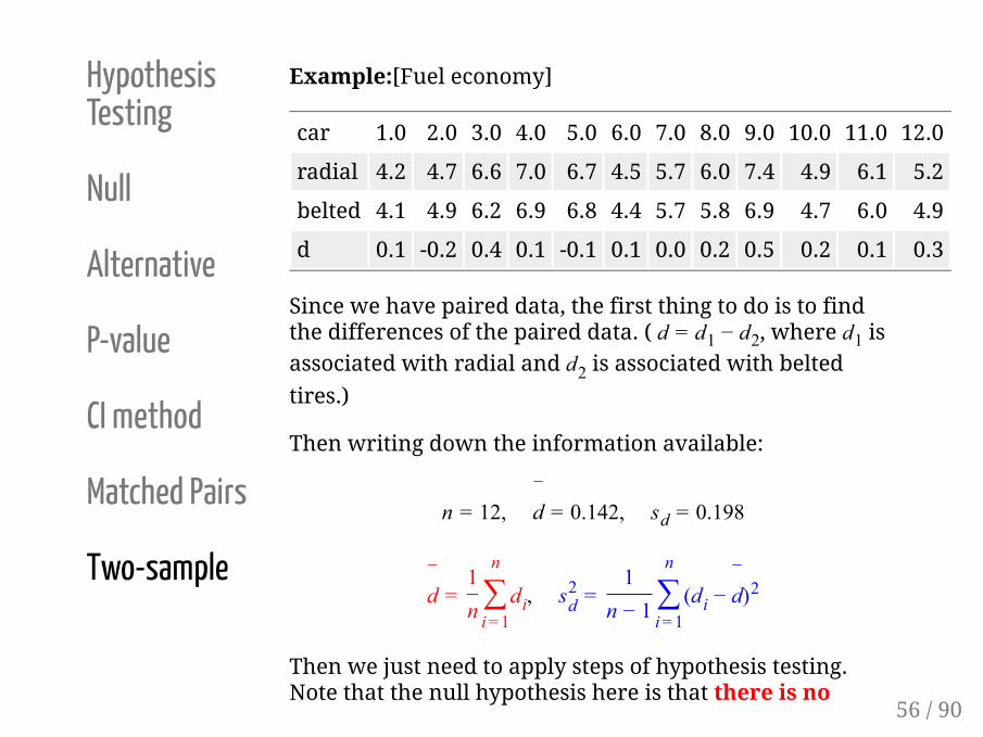
Example:[Fuel economy]
Twelve cars were equipped with radial tires and drivenover a test course. Then the same twelve cars (with thesame drivers) were equipped with regular belted tires anddriven over the same course.
After each run, the cars gas economy (in km/l) wasmeasured. Using significance level α = 0.05 and the methodof critical values, test for a difference in fuel economybetween the radial tires and belted tires.
Construct a 95% confidence interval for true meandifference due to tire type. (i.e μd)
car 1.0 2.0 3.0 4.0 5.0 6.0 7.0 8.0 9.0 10.0 11.0 12.0
radial 4.2 4.7 6.6 7.0 6.7 4.5 5.7 6.0 7.4 4.9 6.1 5.2
belted 4.1 4.9 6.2 6.9 6.8 4.4 5.7 5.8 6.9 4.7 6.0 4.9
55 / 90
HypothesisTesting
Null
Alternative
P-value
CI method
Matched Pairs
Two-sample
Example:[Fuel economy]
car 1.0 2.0 3.0 4.0 5.0 6.0 7.0 8.0 9.0 10.0 11.0 12.0
radial 4.2 4.7 6.6 7.0 6.7 4.5 5.7 6.0 7.4 4.9 6.1 5.2
belted 4.1 4.9 6.2 6.9 6.8 4.4 5.7 5.8 6.9 4.7 6.0 4.9
d 0.1 -0.2 0.4 0.1 -0.1 0.1 0.0 0.2 0.5 0.2 0.1 0.3
Since we have paired data, the first thing to do is to findthe differences of the paired data. ( d = d1 − d2, where d1 isassociated with radial and d2 is associated with belted
tires.)
Then writing down the information available:
n = 12,¯d = 0.142, sd = 0.198
¯d =
1n
n
∑i= 1di, s2
d =1
n − 1
n
∑i= 1
(di −¯d)2
Then we just need to apply steps of hypothesis testing.Note that the null hypothesis here is that there is no
56 / 90

HypothesisTesting
Null
Alternative
P-value
CI method
Matched Pairs
Two-sample
Example:[Fuel economy]
1- H0 : μd = 0 vs. H1 : μd ≠ 0
2- α = 0.05
3- I will use the test statistics K =
¯d− 0
sd / √n which
has a tn− 1 distribution assuming that
H0 is true and
d1, d2, ⋯, d12 are iid N(μd, σ2d)
57 / 90

HypothesisTesting
Null
Alternative
P-value
CI method
Matched Pairs
Two-sample
Example:[Breaking strength of wire, cont'd]
4- K =0.421
0.198 / √12= 2.48 ∼ t ( 11 , 0.975 ) .
p − value = P( | T | > K) = P( | T | > 2.48)= P(T > 2.48) + P(T < − 2.48)= 1 − P(T < 2.48) + P(T < − 2.48)
(by software) = 1 − 0.9847 + 0.9694 = 0.03
5- Since p-value < 0.05, we reject H0.
6- There is enough evidence to conclude thatfuel economy differs between radial and beltedtires.
58 / 90
HypothesisTesting
Null
Alternative
P-value
CI method
Matched Pairs
Two-sample
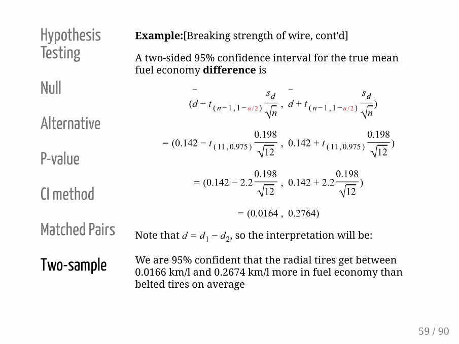
Example:[Breaking strength of wire, cont'd]
A two-sided 95% confidence interval for the true meanfuel economy difference is
(¯d − t (n− 1 , 1 − α / 2 )
sd
√n ,
¯d + t (n− 1 , 1 − α / 2 )
sd
√n)
= (0.142 − t ( 11 , 0.975 )0.198
√12 , 0.142 + t ( 11 , 0.975 )
0.198
√12)
= (0.142 − 2.20.198
√12 , 0.142 + 2.2
0.198
√12)
= (0.0164 , 0.2764)
Note that d = d1 − d2, so the interpretation will be:
We are 95% confident that the radial tires get between0.0166 km/l and 0.2674 km/l more in fuel economy thanbelted tires on average
59 / 90

Hang on for a SecondHang on for a SecondLet's review slide 58 againLet's review slide 58 again
60 / 9060 / 90

HypothesisTesting
Null
Alternative
P-value
CI method
Matched Pairs
Two-sample
Example:[Breaking strength of wire, cont'd]
p − value = P( | T | > K) = P( | T | > 2.48)= P(T > 2.48) + P(T < − 2.48)= 1 − P(T < 2.48) + P(T < − 2.48)
(by software) = 1 − 0.9847 + 0.9694 = 0.03
61 / 90

We have seen t-student tableWe have seen t-student table
How do we get that p-value using How do we get that p-value using softwaresoftware !!! !!!
62 / 9062 / 90

What is happening?What is happening?
63 / 9063 / 90

HypothesisTesting
Null
Alternative
P-value
CI method
Matched Pairs
Two-sample
Unlike standard Normal distribution tablewhich gives us probability under the standardNormal curve, t tables are quantile tables.
i.e We use the t table (Table B.4 in Vardemanand Jobe) to calculate quantiles.
To have exact probabilities, we need software.
64 / 90

The approach in calculating p-value whenThe approach in calculating p-value when
t distribution is involvedt distribution is involved
65 / 9065 / 90

HypothesisTesting
Null
Alternative
P-value
CI method
Matched Pairs
Two-sample
Two important points:
P-value and α are both probabilities. (so ∈ [0, 1]).
They are areas under the curve in tails undernull hypothesis.
66 / 90
HypothesisTesting
Null
Alternative
P-value
CI method
Matched Pairs
Two-sample
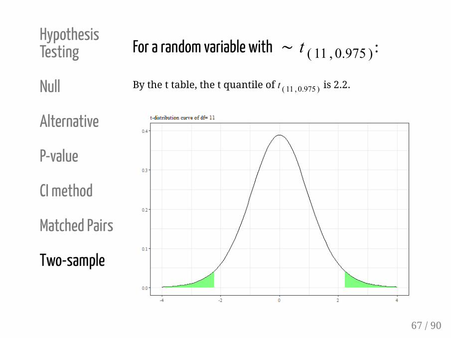
For a random variable with ∼ t ( 11 , 0.975 ) :
By the t table, the t quantile of t ( 11 , 0.975 ) is 2.2.
67 / 90

HypothesisTesting
Null
Alternative
P-value
CI method
Matched Pairs
Two-sample
For the critical value we calculated under the nullhypothesis:
The critical value calculated is K = 2.34
68 / 90

HypothesisTesting
Null
Alternative
P-value
CI method
Matched Pairs
Two-sample
Both together
We reject the null if p-value < α.
Remember p-value and α are areas under thecurve 69 / 90

HypothesisTesting
Null
Alternative
P-value
CI method
Matched Pairs
Two-sample
Example:[End-cut router]
Consider the operation of an end-cut router in themanufacture of a company's wood product. Both aleading-edge and a trailing-edge measurement were madeon each wooden piece to come off the router.
Is the leading-edge measurement different from thetrailing-edge measurement for a typical wood piece?
Do a hypothesis test at α = 0.05 to find out. Make a two-sided 95% confidence interval for the true mean of thedifference between the measurements.
piece 1.000 2.000 3.000 4.000 5.000
leading_edge 0.168 0.170 0.165 0.165 0.170
trailing_edge 0.169 0.168 0.168 0.168 0.169
70 / 90

Two-Sample DataTwo-Sample Data
71 / 9071 / 90

HypothesisTesting
Null
Alternative
P-value
CI method
Matched Pairs
Two-sample
Two-sample data
Paired differences provide inference methods of a specialkind for comparison. Methods that can be used tocompare two means where two different unrelatedsamples will be discussed next.
SAT score of high school A vs. high school B
Severity of a disease in men vs. women
Height of Liverpool soccerr players vs. ManUnited soccer players
Fuel economy of gas formula type A vs.formula type B
72 / 90

HypothesisTesting
Null
Alternative
P-value
CI method
Matched Pairs
Two-sample
Two-sample data
Notations:
73 / 90

Large SamplesLarge Samples
74 / 9074 / 90

HypothesisTesting
Null
Alternative
P-value
CI method
Matched Pairs
Two-sample
Large samples (n1 ≥ 25, n2 ≥ 25)
The difference in sample means ¯x1 −
¯x2 is a natural statistic
to use in comparing μ1 and μ2.
i.e
E(¯X1) = μ1 E(
¯X2) = μ2 Var(
¯X1) =
σ21
n1 Var(
¯X2) =
σ22
n2
If σ1 and σ2 are known, then we have
E(¯X1 −
¯X2) = E(
¯X1) − E(
¯X2) = μ1 − μ2
Var(¯X1 −
¯X2) = Var(
¯X1) + Var(
¯X2) =
σ21
n1+σ2
2
n2
75 / 90

HypothesisTesting
Null
Alternative
P-value
CI method
Matched Pairs
Two-sample
Large samples (n1 ≥ 25, n2 ≥ 25)
If, in addition, n1 and n2 are large,
¯X1 ∼ N(μ1,
σ21
n1) is independent of
¯X2 ∼ N(μ2,
σ22
n2) (by CLT).
So that ¯X1 −
¯X2 is approximately Normal (trust me)
Z =
¯X1 −
¯X2 − (μ1 − μ2)
σ21
n1+σ2
2
n2
∼ N(0, 1)
√
76 / 90
HypothesisTesting
Null
Alternative
P-value
CI method
Matched Pairs
Two-sample
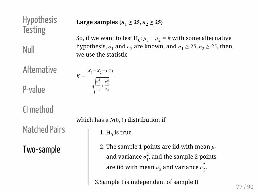
Large samples (n1 ≥ 25, n2 ≥ 25)
So, if we want to test H0 : μ1 − μ2 = # with some alternativehypothesis, σ1 and σ2 are known, and n1 ≥ 25, n2 ≥ 25, thenwe use the statistic
K =
¯X1 −
¯X2 − ( # )
σ21
n1+σ2
2
n2
which has a N(0, 1) distribution if
1. H0 is true
2. The sample 1 points are iid with mean μ1
and variance σ21, and the sample 2 points
are iid with mean μ2 and variance σ22.
3.Sample I is independent of sample II
√
77 / 90

HypothesisTesting
Null
Alternative
P-value
CI method
Matched Pairs
Two-sample
Large samples (n1 ≥ 25, n2 ≥ 25)
The confidence intervals (2-sided, 1-sided upper, and 1-sided lower, respectively) for μ1 − μ2 are:
Two-sided 100(1 − α)% confidence interval for μ1 − μ2
(¯x1 −
¯x2) ± z1 −α / 2 ∗
σ21
n1+σ2
2
n2
One-sided 100(1 − α)% confidence interval for μ1 − μ2with a upper confidence bound
( − ∞ , (¯x1 −
¯x2) ± z1 − α ∗
σ21
n1+σ2
2
n2)
One-sided 100(1 − α)% confidence interval for μ with alower confidence bound
√
√
78 / 90

HypothesisTesting
Null
Alternative
P-value
CI method
Matched Pairs
Two-sample
Large samples (n1 ≥ 25, n2 ≥ 25)
If σ1 and σ2 are unknown, and n1 ≥ 25, n2 ≥ 25, then we usethe statistic
K =
¯X1 −
¯X2 − ( # )
σ21
n1+σ2
2
n2
and confidence intervals (2-sided, 1-sided upper, and 1-sided lower, respectively) for μ1 − μ2:
Two-sided 100(1 − α)% confidence interval for μ1 − μ2
(¯x1 −
¯x2) ± z1 −α / 2 ∗
s21
n1+s2
2
n2
√
√
79 / 90
HypothesisTesting
Null
Alternative
P-value
CI method
Matched Pairs
Two-sample
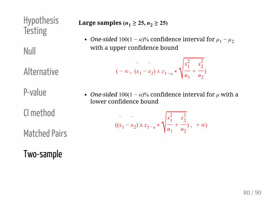
Large samples (n1 ≥ 25, n2 ≥ 25)
One-sided 100(1 − α)% confidence interval for μ1 − μ2with a upper confidence bound
( − ∞ , (¯x1 −
¯x2) ± z1 − α ∗
s21
n1+s2
2
n2)
One-sided 100(1 − α)% confidence interval for μ with alower confidence bound
((¯x1 −
¯x2) ± z1 − α ∗
s21
n1+s2
2
n2) , + ∞)
√
√
80 / 90

HypothesisTesting
Null
Alternative
P-value
CI method
Matched Pairs
Two-sample
Example:[Anchor bolts]
An experiment carried out to study various characteristicsof anchor bolts resulted in 78 observations on shearstrength (kip) of 3/8-in. diameter bolts and 88 observationson strength of 1/2-in. diameter bolts.
Let Sample 1 be the 1/2 in diameter bolts and Sample 2 bethe 3/8 indiameter bolts.
Using a significance level of α = 0.01, find out if the 1/2 inbolts are more than 2 kip stronger (in shear strength) thanthe 3/8 in bolts. Calculate and interpret the appropriate99% confidence interval to support the analysis.
n1 = 88, n2 = 78
¯x1 = 7.14,
¯x2 = 4.25
s1 = 1.68, s2 = 1.3
81 / 90

HypothesisTesting
Null
Alternative
P-value
CI method
Matched Pairs
Two-sample
Example:[Anchor bolts]
n1 = 88, n2 = 78
¯x1 = 7.14,
¯x2 = 4.25
s1 = 1.68, s2 = 1.3
82 / 90

Small SamplesSmall Samples
83 / 9083 / 90

HypothesisTesting
Null
Alternative
P-value
CI method
Matched Pairs
Two-sample
Small samples
If n1 < 25 or n2 < 25, then we need some other
assumptions to hold in order to complete inference ontwo-sample data.
We need two independent samples to be iidNormally distributed and σ2
1 ≈ σ22
A test statistic to test H0 : μ1 − μ2 = # against somealternative is
K =
¯X1 −
¯X2 − (#)
Sp (1n1
+1n2
)
where S2p is called pooled sample variance and is defined
as
S2p =
(n1 − 1)S21 + (n2 − 1)S2
2
n1 + n2 − 2
√
84 / 90

HypothesisTesting
Null
Alternative
P-value
CI method
Matched Pairs
Two-sample
Small samples
Also assuming
H0 is true,
The sample 1 points are iid N(μ1, σ21), the sample 2
points are iid N(μ2, σ22),
and the sample 1 points are independent of thesample 2 points and σ2
1 ≈ σ22.
Then
K =
¯X1 −
¯X2 − (#)
Sp (1n1
+1n2
)∼ t (n1 +n2 − 2 )
√
85 / 90

HypothesisTesting
Null
Alternative
P-value
CI method
Matched Pairs
Two-sample
Small samples
1 − α confidence intervals (2-sided, 1-sided upper, and 1-sided lower, respectively) for μ1 − μ2 under these
assumptions are of the form:
(let ν = n1 + n2 − 2)
Two-sided 100(1 − α)% confidence interval for μ1 − μ2
(¯x1 −
¯x2) ± t ( ν , 1 −α / 2 ) ∗ Sp (
1n1
+1n2
)
One-sided 100(1 − α)% confidence interval for μ1 − μ2with a upper confidence bound
( − ∞ , (¯x1 −
¯x2) + t ( ν , 1 − α ) ∗ Sp (
1n1
+1n2
)
√
√
86 / 90

HypothesisTesting
Null
Alternative
P-value
CI method
Matched Pairs
Two-sample
Small samples
One-sided 100(1 − α)% confidence interval for μ with alower confidence bound
((¯x1 −
¯x2) − t ( ν , 1 − α ) ∗ Sp (
1n1
+1n2
) , + ∞)√
87 / 90

HypothesisTesting
Null
Alternative
P-value
CI method
Matched Pairs
Two-sample
Small samples
Example:[Springs]
The data of W. Armstrong on spring lifetimes (appearingin the book by Cox and Oakes) not only concern springlongevity at a 950 N/ mm2 stress level but also longevity ata 900 N/ mm2 stress level.
Let sample 1 be the 900 N/ mm2 stress group and sample 2be the 950 N/ mm2 stress group.
900 N/mm2 Stress 950 N/mm2 Stress
216, 162, 153, 216, 225, 216,306, 225, 243, 189
225, 171, 198, 189, 189, 135,162, 135, 117, 162
88 / 90

HypothesisTesting
Null
Alternative
P-value
CI method
Matched Pairs
Two-sample
Small samples
Example:[Springs]
Let's do a hypothesis test to see if the sample 1 springslasted significantly longer than the sample 2 springs.
89 / 90

HypothesisTesting
Null
Alternative
P-value
CI method
Matched Pairs
Two-sample
Small samples
Example:[Stopping distance]
Suppose μ1 and μ2 are true mean stopping distances (in
meters) at 50 mph for cars of a certain type equipped withtwo different types of breaking systems.
Suppose n1 = n2 = 6, ¯x1 = 115.7,
¯x2 = 129.3, s1 = 5.08, and
s2 = 5.38.
Use significance level α = 0.01 to test H0 : μ1 − μ2 = − 10 vs.
HA : μ1 − μ2 < − 10.
Construct a 2-sided 99% confidence interval for the truedifference in stopping distances.
90 / 90