Hypothesis Testing For Densities andHigh-Dimensional Multinomials: Sharp Local Minimax Rates

Sivaraman Balakrishnan† Larry Wasserman†

Department of Statistics†

Carnegie Mellon UniversityPittsburgh, PA 15213

{siva,larry}@stat.cmu.edu

June 29, 2017

Abstract

We consider the goodness-of-fit testing problem of distinguishing whether the data aredrawn from a specified distribution, versus a composite alternative separated from the nullin the total variation metric. In the discrete case, we consider goodness-of-fit testing whenthe null distribution has a possibly growing or unbounded number of categories. In thecontinuous case, we consider testing a Lipschitz density, with possibly unbounded support,in the low-smoothness regime where the Lipschitz parameter is not assumed to be constant.In contrast to existing results, we show that the minimax rate and critical testing radiusin these settings depend strongly, and in a precise way, on the null distribution beingtested and this motivates the study of the (local) minimax rate as a function of the nulldistribution. For multinomials the local minimax rate was recently studied in the work ofValiant and Valiant [30]. We re-visit and extend their results and develop two modificationsto the χ2-test whose performance we characterize. For testing Lipschitz densities, we showthat the usual binning tests are inadequate in the low-smoothness regime and we design aspatially adaptive partitioning scheme that forms the basis for our locally minimax optimaltests. Furthermore, we provide the first local minimax lower bounds for this problemwhich yield a sharp characterization of the dependence of the critical radius on the nullhypothesis being tested. In the low-smoothness regime we also provide adaptive tests, thatadapt to the unknown smoothness parameter. We illustrate our results with a variety ofsimulations that demonstrate the practical utility of our proposed tests.

1 Introduction

Hypothesis testing is one of the pillars of modern mathematical statistics with a vast array ofscientific applications. There is a well-developed theory of hypothesis testing starting with thework of Neyman and Pearson [22], and their framework plays a central role in the theory andpractice of statistics. In this paper we re-visit the classical goodness-of-fit testing problem ofdistinguishing the hypotheses:

H0 : Z1, . . . , Zn ∼ P0 versus H1 : Z1, . . . , Zn ∼ P ∈ A (1)

for some set of distributions A. This fundamental problem has been widely studied (see forinstance [19] and references therein).

A natural choice of the composite alternative, one that has a clear probabilistic inter-pretation, excludes a total variation neighborhood around the null, i.e. we take A = {P :

1

TV(P, P0) ≥ ε/2}. This is equivalent to A = {P : ‖P − P0‖1 ≥ ε}, and we use this representa-tion in the rest of this paper. However, there exist no consistent tests that can distinguishan arbitrary distribution P0 from alternatives separated in `1; see [2, 17]. Hence, we imposestructural restrictions on P0 and A. We focus on two cases:

1. Multinomial testing: When the null and alternate distributions are multinomials.

2. Lipschitz testing: When the null and alternate distributions have Lipschitz densities.

The problem of goodness-of-fit testing for multinomials has a rich history in statistics andpopular approaches are based on the χ2-test [24] or the likelihood ratio test [5, 22, 32]; see,for instance, [9, 11, 21, 23, 25] and references therein. Motivated by connections to propertytesting [26], there is also a recent literature developing in computer science; see [3, 10, 13, 30].Testing Lipschitz densities is one of the basic non-parametric hypothesis testing problems andtests are often based on the Kolmogorov-Smirnov or Cramer-von Mises statistics [7, 27, 31].This problem was originally studied from the minimax perspective in the work of Ingster[14, 15]. See [1, 12, 14] for further references.

In the goodness-of-fit testing problem in (1), previous results use the (global) critical radiusas a benchmark. Roughly, this global critical radius is a measure of the minimal separationbetween the null and alternate hypotheses that ensures distinguishability, as the null hypothesisis varied over a large class of distributions (for instance over the class of distributions withLipschitz densities or over the class of all multinomials on d categories). Remarkably, as shownin the work of Valiant and Valiant [30] for the case of multinomials and as we show in this paperfor the case of Lipschitz densities, there is considerable heterogeneity in the critical radiusas a function of the null distribution P0. In other words, even within the class of Lipschitzdensities, testing certain null hypotheses can be much easier than testing others. Consequently,the local minimax rate which describes the critical radius for each individual null distributionprovides a much more nuanced picture. In this paper, we provide (near) matching upper andlower bounds on the critical radii for Lipschitz testing as a function of the null distribution,i.e. we precisely upper and lower bound the critical radius for each individual Lipschitz nullhypothesis. Our upper bounds are based on χ2-type tests, performed on a carefully chosenspatially adaptive binning, and highlight the fact that the standard prescriptions of choosingbins with a fixed width [28] can yield sub-optimal tests.

The distinction between local and global perspectives is reminiscent of similar effectsthat arise in some estimation problems, for instance in shape-constrained inference [4], inconstrained least-squares problems [6] and in classical Fisher Information-Cramer-Rao bounds[18].

The remainder of this paper is organized as follows. In Section 2 we provide somebackground on the minimax perspective on hypothesis testing, and formally describe thelocal and global minimax rates. We provide a detailed discussion of the problem of studyand finally provide an overview of our main results. In Section 3 we review the results of[30] and present a new globally-minimax test for testing multinomials, as well as a (nearly)locally-minimax test. In Section 4 we consider the problem of testing a Lipschitz densityagainst a total variation neighbourhood. We present the body of our main technical result inSection 4.3 and defer technical aspects of this proof to the Appendix. In each of Section 3and 4 we present simulation results that demonstrate the superiority of the tests we proposeand their potential practical applicability. In the Appendix, we also present several otherresults including a brief study of limiting distributions of the test statistics under the null, aswell as tests that are adaptive to various parameters.

2

2 Background and Problem Setup

We begin with some basic background on hypothesis testing, the testing risk and minimaxrates, before providing a detailed treatment of some related work.

2.1 Hypothesis testing and minimax rates

Our focus in this paper is on the one sample goodness-of-fit testing problem. We observesamples Z1, . . . , Zn ∈ X , where X ⊂ Rd, which are independent and identically distributedwith distribution P . In this context, for a fixed distribution P0, we want to test the hypotheses:

H0 : P = P0 versus

H1 : ‖P − P0‖1 ≥ εn.(2)

Throughout this paper we use P0 to denote the null distribution and P to denote an arbi-trary alternate distribution. Throughout the paper, we use the total variation distance (orequivalently the `1 distance) between two distributions P and Q, defined by

TV(P,Q) = supA|P (A)−Q(A)| (3)

where the supremum is over all measurable sets. If P and Q have densities p and q withrespect to a common dominating measure ν, then

TV(P,Q) =1

2

∫|p− q|dν =

1

2‖p− q‖1 ≡

1

2‖P −Q‖1. (4)

We consider the total variation distance because it has a clear probabilistic meaning andbecause it is invariant under one-to-one transformations [8]. The `2 metric is often easier towork with but in the context of distribution testing its interpretation is less intuitive. Ofcourse, other metrics (for instance Hellinger, χ2 or Kullback-Leibler) can be used as well butwe focus on TV (or `1) throughout this paper. It is well-understood [2, 17] that withoutfurther restrictions there are no uniformly consistent tests for distinguishing these hypotheses.Consequently, we focus on two restricted variants of this problem:

1. Multinomial testing: In the multinomial testing problem, the domain of the distributionsis X = {1, . . . , d} and the distributions P0 and P are equivalently characterized byvectors p0, p ∈ Rd. Formally, we define,

M ={p : p ∈ Rd,

d∑i=1

pi = 1, pi ≥ 0 ∀ i ∈ {1, . . . , d}},

and consider the multinomial testing problem of distinguishing:

H0 : P = P0, P0 ∈M versus H1 : ‖P − P0‖1 ≥ εn, P ∈M. (5)

In contrast to classical “fixed-cells” asymptotic theory [25], we focus on high-dimensionalmultinomials where d can grow with, and potentially exceed the sample size n.

2. Lipschitz testing: In the Lipschitz density testing problem the set X ⊂ Rd, and werestrict our attention to distributions with Lipschitz densities, i.e. letting p0 and p denote

3

the densities of P0 and P with respect to the Lebesgue measure, we consider the set ofdensities:

L(Ln) =

{p :

∫Xp(x)dx = 1, p(x) ≥ 0 ∀ x, |p(x)− p(y)| ≤ Ln‖x− y‖2 ∀ x, y ∈ Rd

},

and consider the Lipschitz testing problem of distinguishing:

H0 : P = P0, P0 ∈ L(Ln) versus H1 : ‖P − P0‖1 ≥ εn, P ∈ L(Ln). (6)

We emphasize, that unlike prior work [1, 12, 15] we do not require p0 to be uniform.We also do not restrict the domain of the densities and we consider the low-smoothnessregime where the Lipschitz parameter Ln is allowed to grow with the sample size.

Hypothesis testing and risk. Returning to the setting described in (2), we define a test φas a Borel measurable map, φ : X n 7→ {0, 1}. For a fixed null distribution P0, we define the setof level α tests:

Φn,α ={φ : Pn0 (φ = 1) ≤ α

}. (7)

The worst-case risk (type II error) of a test φ over a restricted class C which contains P0 is

Rn(φ;P0, εn, C) = sup{EP [1− φ] : ‖P − P0‖1 ≥ εn, P ∈ C

}.

The local minimax risk is1:

Rn(P0, εn, C) = infφ∈Φn,α

Rn(φ;P0, εn, C). (8)

It is common to study the minimax risk via a coarse lens by studying instead the criticalradius or the minimax separation. The critical radius is the smallest value εn for which ahypothesis test has non-trivial power to distinguish P0 from the set of alternatives. Formally,we define the local critical radius as:

εn(P0, C) = inf{ε : Rn(P0, εn, C) ≤ 1/2

}. (9)

The constant 1/2 is arbitrary; we could use any number in (0, 1− α).The local minimax risk and critical radius depend on the null distribution P0. A more

common quantity of interest is the global minimax risk

Rn(εn, C) = supP0∈C

Rn(P0, εn, C). (10)

The corresponding global critical radius is

εn(C) = inf{εn : Rn(εn, C) ≤ 1/2

}. (11)

In typical non-parametric problems, the local minimax risk and the global minimax riskmatch up to constants and this has led researchers in past work to focus on the global minimaxrisk. We show that for the distribution testing problems we consider, the local critical radius

1Although our proofs are explicit in their dependence on α, we suppress this dependence in our notationand in our main results treating α as a fixed strictly positive universal constant.

4

in (9) can vary considerably as a function of the null distribution P0. As a result, the globalcritical radius, provides only a partial understanding of the intrinsic difficulty of this family ofhypothesis testing problems. In this paper, we focus on producing tight bounds on the localminimax separation. These bounds yield as a simple corollary, sharp bounds on the globalminimax separation, but are in general considerably more refined.

Poissonization: In constructing upper bounds on the minimax risk—we work under asimplifying assumption that the sample size is random: n0 ∼ Poisson(n). This assumption isstandard in the literature [1, 30], and simplifies several calculations. When the sample size ischosen to be distributed as Poisson(n), it is straightforward to verify that for any fixed setA,B ⊂ X with A ∩B = ∅, under P the number of samples falling in A and B are distributedindependently as Poisson(nP (A)) and Poisson(nP (B)) respectively.

In the Poissonized setting, we consider the averaged minimax risk, where we additionallyaverage the risk in (8) over the random sample size. The Poisson distribution is tightlyconcentrated around its mean and this additional averaging only affects constant factors inthe minimax risk and we ignore this averaging in the rest of the paper.

2.2 Overview of our results

With the basic framework in place we now provide a high-level overview of the main results ofthis paper. In the context of testing multinomials, the results of [30] characterize the localand global minimax rates. We provide the following additional results:

• In Theorem 2 we characterize a simple and practical globally minimax test. In Theorem 4building on the results of [10] we provide a simple (near) locally minimax test.

In the context of testing Lipschitz densities we make advances over classical results [12, 14]by eliminating several unnecessary assumptions (uniform null, bounded support, fixed Lipschitzparameter). We provide the first characterization of the local minimax rate for this problem.In studying the Lipschitz testing problem in its full generality we find that the critical testingradius can exhibit a wide range of possible behaviours, based roughly on the tail behaviour ofthe null hypothesis.

• In Theorem 5 we provide a characterization of the local minimax rate for Lipschitz densitytesting. In Section 4.1, we consider a variety of concrete examples that demonstrate therich scaling behaviour exhibited by the critical radius in this problem.

• Our upper and lower bounds are based on a novel spatially adaptive partitioning scheme.We describe this scheme and derive some of its useful properties in Section 4.2.

In the Supplementary Material we provide the technical details of the proofs. We brieflyconsider the limiting behaviour of our test statistics under the null in Appendix A. Our resultsshow that the critical radius is determined by a certain functional of the null hypothesis. InAppendix D we study certain important properties of this functional pertaining to its stability.Finally, we study tests which are adaptive to various parameters in Appendix F.

3 Testing high-dimensional multinomials

Given a sample Z1, . . . , Zn ∼ P define the counts X = (X1, . . . , Xd) where Xj =∑n

i=1 I(Zi =j). The local minimax critical radii for the multinomial problem have been found in Valiantand Valiant [30]. We begin by summarizing these results.

5

Without loss of generality we assume that the entries of the null multinomial p0 are sortedso that p0(1) ≥ p0(2) ≥ . . . ≥ p0(d). For any 0 ≤ σ ≤ 1 we denote σ-tail of the multinomial by:

Qσ(p0) =

i :

d∑j=i

p0(j) ≤ σ

. (12)

The σ-bulk is defined to be

Bσ(p0) = {i > 1 : i /∈ Qσ(p0)}. (13)

Note that i = 1 is excluded from the σ-bulk. The minimax rate depends on the functional:

Vσ(p0) =

∑i∈Bσ(p0)

p0(i)2/3

3/2

. (14)

For a given multinomial p0, our goal is to upper and lower bound the local critical radiusεn(p0,M) in (9). We define, `n and un to be the solutions to the equations 2:

`n(p0) = max

{1

n,

√V`n(p0)(p0)

n

}, un(p0) = max

{1

n,

√Vun(p0)/16(p0)

n

}. (15)

With these definitions in place, we are now ready to state the result of [30]. We usec1, c2, C1, C2 > 0 to denote positive universal constants.

Theorem 1 ([30]). The local critical radius εn(p0,M) for multinomial testing is upper andlower bounded as:

c1`n(p0) ≤ εn(p0,M) ≤ C1un(p0). (16)

Furthermore, the global critical radius εn(M) is bounded as:

c2d1/4

√n≤ εn(M) ≤ C2d

1/4

√n

.

Remarks:

• The local critical radius is roughly determined by the (truncated) 2/3-rd norm of themultinomial p0. This norm is maximized when p0 is uniform and is small when p0 issparse, and at a high-level captures the “effective sparsity” of p0.

• The global critical radius can shrink to zero even when d� n. When d �√n almost all

categories of the multinomial are unobserved but it is still possible to reliably distinguishany p0 from an `1-neighborhood. This phenomenon is noted for instance in the work of[23]. We also note the work of Barron [2] that shows that when d = ω(n), no test canhave power that approaches 1 at an exponential rate.

2These equations always have a unique solution since the right hand side monotonically decreases to 0 asthe left hand side monotonically increases from 0 to 1.

6

• The local critical radius can be much smaller than the global minimax radius. If themultinomial p0 is nearly (or exactly) s-sparse then the critical radius is upper and lowerbounded up to constants by s1/4/

√n. Furthermore, these results also show that it is

possible to design consistent tests for sufficiently structured null hypotheses: in caseswhen

√d� n, and even in cases when d is infinite.

• Except for certain pathological multinomials, the upper and lower critical radii match upto constants. We revisit this issue in Appendix D, in the context of Lipschitz densities,where we present examples where the solutions to critical equations similar to (15) arestable and examples where they are unstable.

In the remainder of this section we consider a variety of tests, including the test presented in[30] and several alternatives. The test of [30] is a composite test that requires knowledge of εnand the analysis of their test is quite intricate. We present an alternative, simple test that isglobally minimax, and then present an alternative composite test that is locally minimax butsimpler to analyze. Finally, we present a few illustrative simulations.

3.1 The truncated χ2 test

We begin with a simple globally minimax test. From a practical standpoint, the most populartest for multinomials is Pearson’s χ2 test. However, in the high-dimensional regime where thedimension of the multinomial d is not treated as fixed the χ2 test can have bad power due tothe fact that the variance of the χ2 statistic is dominated by small entries of the multinomial(see [20, 30]).

A natural thought then is to truncate the normalization factors of the χ2 statistic in orderto limit the contribution to the variance from each cell of the multinomial. Recalling that(X1, . . . , Xd) denote the observed counts, we propose the test statistic:

Ttrunc =d∑i=1

(Xi − np0(i))2 −Xi

max{1/d, p0(i)}:=

d∑i=1

(Xi − np0(i))2 −Xi

θi(17)

and the corresponding test,

φtrunc = I

Ttrunc > n

√√√√ 2

α

d∑i=1

p0(i)2

θ2i

. (18)

This test statistic truncates the usual normalization factor for the χ2 test for any entry whichfalls below 1/d, and thus ensures that very small entries in p0 do not have a large effect on thevariance of the statistic. We emphasize the simplicity and practicality of this test. We havethe following result which bounds the power and size of the truncated χ2 test. We use C > 0to denote a positive universal constant.

Theorem 2. Consider the testing problem in (5). The truncated χ2 test has size at most α,i.e. P0(φtrunc = 1) ≤ α. Furthermore, there is a universal constant C > 0 such that if for any0 < ζ ≤ 1 we have that,

ε2n ≥C√d

n

[1√α

+1

ζ

], (19)

then the Type II error of the test is bounded by ζ, i.e. P (φtrunc = 0) ≤ ζ.

7

Remarks:

• A straightforward consequence of this result together with the result in Theorem 1 isthat the truncated χ2 test is globally minimax optimal.

• The classical χ2 and likelihood ratio tests are not generally consistent (and thus notglobally minimax optimal) in the high-dimensional regime (see also, Figure 2).

• At a high-level the proof follows by verifying that when the alternate hypothesis is true,under the condition on the critical radius in (19), the test statistic is larger than thethreshold in (18). To verify this, we lower bound the mean and upper bound the varianceof the test statistic under the alternate and then use standard concentration results. Wedefer the details to the Supplementary Material (Appendix B).

3.2 The 2/3-rd + tail test

The truncated χ2 test described in the previous section, although globally minimax, is notlocally adaptive. The test from [30], achieves the local minimax upper bound in Theorem 1.We refer to this as the 2/3-rd + tail test. We use a slightly modified version of their test whentesting Lipschitz goodness-of-fit in Section 4, and provide a description here.

The test is a composite two-stage test, and has a tuning parameter σ. Recalling thedefinitions of Bσ(p0) andQσ(p0) (see (12)), we define two test statistics T1, T2 and correspondingtest thresholds t1, t2:

T1(σ) =∑

j∈Qσ(p0)

(Xj − np0(j)), t1(α, σ) =

√nP0(Qσ(p0))

α,

T2(σ) =∑

j∈Bσ(p0)

(Xj − np0(j))2 −Xj

p2/3j

, t2(α, σ) =

√∑j∈Bσ 2n2p0(j)2/3

α.

We define two tests:

1. The tail test: φtail(σ, α) = I(T1(σ) > t1(α, σ)).

2. The 2/3-test: φ2/3(σ, α) = I(T2(σ) > t2(α, σ)).

The composite test φV (σ, α) is then given as:

φV (σ, α) = max{φtail(σ, α/2), φ2/3(σ, α/2)}. (20)

With these definitions in place, the following result is essentially from the work of [30]. Weuse C > 0 to denote a positive universal constant.

Theorem 3. Consider the testing problem in (5). The composite test φV (σ, α) has size atmost α, i.e. P0(φV = 1) ≤ α. Furthermore, if we choose σ = εn(p0,M)/8, and un(p0) asin (15), then for any 0 < ζ ≤ 1, if

εn(p0,M) ≥ Cun(p0) max{1/α, 1/ζ}, (21)

then the Type II error of the test is bounded by ζ, i.e. P (φV = 0) ≤ ζ.

Remarks:

8

• The test φV is also motivated by deficiencies of the χ2 test. In particular, the testincludes two main modifications to the χ2 test which limit the contribution of the smallentries of p0: some of the small entries of p0 are dealt with via a separate tail test andfurther the normalization of the χ2 test is changed from p0(i) to p0(i)2/3.

• This result provides the upper bound of Theorem 1. It requires that the tuning parameterσ is chosen as εn(p0,M)/8. In the Supplementary Material (Appendix F) we discussadaptive choices for σ.

• The proof essentially follows from the paper of [30], but we maintain an explicit boundon the power and size of the test, which we use in later sections. We provide the detailsin Appendix B.

While the 2/3-rd norm test is locally minimax optimal its analysis is quite challenging. In thenext section, we build on results from a recent paper of Diakonikolas and Kane [10] to providean alternative (nearly) locally minimax test with a simpler analysis.

3.3 The Max Test

An important insight, one that is seen for instance in Figure 1, is that many simple tests areoptimal when p0 is uniform and that careful modifications to the χ2 test are required onlywhen p0 is far from uniform. This suggests the following strategy: partition the multinomialinto nearly uniform groups, apply a simple test within each group and combine the tests withan appropriate Bonferroni correction. We refer to this as the max test. Such a strategy wasused by Diakonikolas and Kane [10], but their test is quite complicated and involves manyconstants. Furthermore, it is not clear how to ensure that their test controls the Type I errorat level α. Motivated by their approach, we present a simple test that controls the type I erroras required and is (nearly) locally minimax.

As with the test in the previous section, the test has to be combined with the tail test.The test is defined to be

φmax(σ, α) = max{φtail(σ, α/2), φM (σ, α/2)},

where φM is defined as follows. We partition Bσ(p0) into sets Sj for j ≥ 1, where

Sj ={t :

p0(2)

2j< p0(t) ≤ p0(2)

2j−1

}.

We can bound the total number of sets Sj by noting that for any i ∈ Bσ(p0), we have thatp0(i) ≥ σ/d, so that the number of sets k is bounded by dlog2(d/σ)e. Within each set we usea modified `2 statistic. Let

Tj =∑t∈Sj

[(Xt − np0(t))2 −Xt] (22)

for j ≥ 1. Unlike the traditional `2 statistic, each term in this statistic is centered around Xt.As observed in [30], this results in the statistic having smaller variance in the n� d regime.Let

φM (σ, α) =∨j

I(Tj > tj), (23)

9

where

tj =

√√√√2kn2[∑

t∈Sj p0(t)2]

α. (24)

Theorem 4. Consider the testing problem in (5). Suppose we choose σ = εn(p0,M)/8, thenthe composite test φmax(σ, α) has size at most α, i.e. P0(φmax = 1) ≤ α. Furthermore, there isa universal constant C > 0, such that for un(p0) as in (15), if for any 0 < ζ ≤ 1 we have that,

εn(p0,M) ≥ Ck2un(p0) max

{√k

α,

1

ζ

}, (25)

then the Type II error of the test is bounded by ζ, i.e. P (φmax = 0) ≤ ζ.

Remarks:

• Comparing the critical radii in Equations (25) and (16), and noting that k ≤ dlog2(8d/εn)e,we conclude that the max test is locally minimax optimal, up to a logarithmic factor.

• In contrast to the analysis of the 2/3-rd + tail test in [30], the analysis of the maxtest involves mostly elementary calculations. We provide the details in Appendix B.As emphasized in the work of [10], the reduction of testing problems to simpler testingproblems (in this case, testing uniformity) is a more broadly useful idea. Our upperbound for the Lipschitz testing problem (in Section 4) proceeds by reducing it to amultinomial testing problem through a spatially adaptive binning scheme.

3.4 Simulations

In this section, we report some simulation results that demonstrate the practicality of theproposed tests. We focus on two simulation scenarios and compare the globally-minimaxtruncated χ2 test, and the 2/3rd + tail test [30] with the classical χ2-test and the likelihoodratio test. The χ2 statistic is,

Tχ2 =d∑i=1

(Xi − np0(i))2 − np0(i)

np0(i),

and the likelihood ratio test statistic is

TLRT = 2d∑i=1

Xi log

(Xi

np0(i)

).

In Appendix G, we consider a few additional simulations as well as a comparison with statisticsbased on the `1 and `2 distances.

In each setting described below, we set the α level threshold via simulation (by samplingfrom the null 1000 times) and we calculate the power under particular alternatives by averagingover a 1000 trials.

10

ℓ1 Distance0 0.2 0.4 0.6 0.8 1

Power

0

0.1

0.2

0.3

0.4

0.5

0.6

0.7

0.8

0.9

1Uniform Null, Dense Alternate

Chi-sq.Truncated chi-sqLRT2/3rd and tail

ℓ1 Distance0 0.1 0.2 0.3 0.4 0.5 0.6 0.7 0.8

Power

0

0.1

0.2

0.3

0.4

0.5

0.6

0.7

0.8

0.9

1Uniform Null, Sparse Alternate

Chi-sq.Truncated chi-sqLRT2/3rd and tail

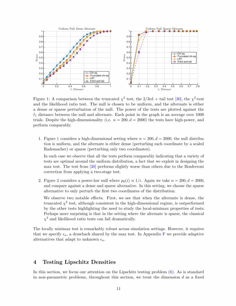
Figure 1: A comparison between the truncated χ2 test, the 2/3rd + tail test [30], the χ2-testand the likelihood ratio test. The null is chosen to be uniform, and the alternate is eithera dense or sparse perturbation of the null. The power of the tests are plotted against the`1 distance between the null and alternate. Each point in the graph is an average over 1000trials. Despite the high-dimensionality (i.e. n = 200, d = 2000) the tests have high-power, andperform comparably.

1. Figure 1 considers a high-dimensional setting where n = 200, d = 2000, the null distribu-tion is uniform, and the alternate is either dense (perturbing each coordinate by a scaledRademacher) or sparse (perturbing only two coordinates).

In each case we observe that all the tests perform comparably indicating that a variety oftests are optimal around the uniform distribution, a fact that we exploit in designing themax test. The test from [30] performs slightly worse than others due to the Bonferronicorrection from applying a two-stage test.

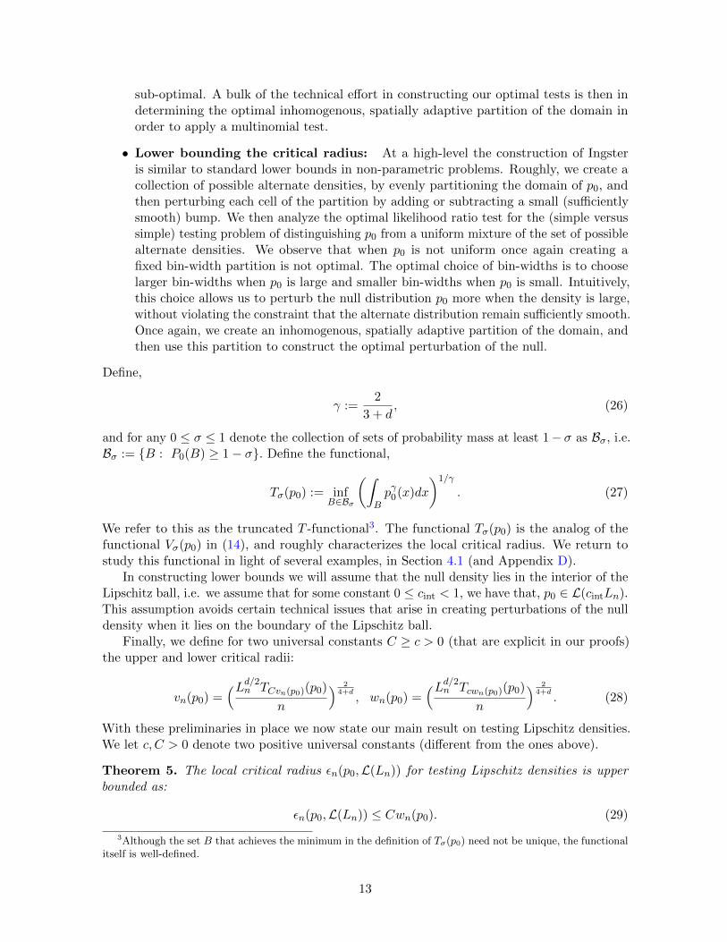
2. Figure 2 considers a power-law null where p0(i) ∝ 1/i. Again we take n = 200, d = 2000,and compare against a dense and sparse alternative. In this setting, we choose the sparsealternative to only perturb the first two coordinates of the distribution.

We observe two notable effects. First, we see that when the alternate is dense, thetruncated χ2 test, although consistent in the high-dimensional regime, is outperformedby the other tests highlighting the need to study the local-minimax properties of tests.Perhaps more surprising is that in the setting where the alternate is sparse, the classicalχ2 and likelihood ratio tests can fail dramatically.

The locally minimax test is remarkably robust across simulation settings. However, it requiresthat we specify εn, a drawback shared by the max test. In Appendix F we provide adaptivealternatives that adapt to unknown εn.

4 Testing Lipschitz Densities

In this section, we focus our attention on the Lipschitz testing problem (6). As is standardin non-parametric problems, throughout this section, we treat the dimension d as a fixed

11

ℓ1 Distance0 0.1 0.2 0.3 0.4 0.5 0.6

Power

0

0.1

0.2

0.3

0.4

0.5

0.6

0.7

0.8

0.9

1Power Law Null, Dense Alternate

Chi-sq.Truncated chi-sqLRT2/3rd and tail

ℓ1 Distance0 0.1 0.2 0.3 0.4 0.5 0.6 0.7 0.8

Power

0

0.1

0.2

0.3

0.4

0.5

0.6

0.7

0.8

0.9

1Power Law Null, Sparse Alternate

Chi-sq.Truncated chi-sqLRT2/3rd and tail

Figure 2: A comparison between the truncated χ2 test, the 2/3rd + tail test [30], the χ2-testand the likelihood ratio test. The null is chosen to be a power law, and the alternate is eithera dense or sparse perturbation of the null. The power of the tests are plotted against the `1distance between the null and alternate. Each point in the graph is an average over 1000 trials.The truncated χ2 test despite being globally minimax optimal, can perform poorly for anyparticular fixed null. The χ2 and likelihood ratio tests can fail to be consistent even when εnis quite large, and n�

√d.

(universal) constant. Our emphasis is on understanding the local critical radius while makingminimal assumptions. In contrast to past work, we do not assume that the null is uniform oreven that its support is compact. We would like to be able to detect more subtle deviationsfrom the null as the sample size gets large and hence we do not assume that the Lipschitzparameter Ln is fixed as n grows.

The classical method, due to Ingster [15, 16] to constructing lower and upper bounds onthe critical radius, is based on binning the domain of the density. In particular, upper boundswere obtained by considering χ2 tests applied to the multinomial that results from binningthe null distribution. Ingster focused on the case when the null distribution P0 was taken tobe uniform on [0, 1], noting that the testing problem for a general null distribution could be“reduced” to testing uniformity by modifying the observations via the quantile transformationcorresponding to the null distribution P0 (see also [12]). We emphasize that such a reductionalters the smoothness class tailoring it to the null distribution P0. The quantile transformationforces the deviations from the null distribution to be more smooth in regions where P0 is smalland less smooth where P0 is large, i.e. we need to re-interpret smoothness of the alternativedensity p as an assumption about the function p(F−1

0 (t)), where F−10 is the quantile function of

the null distribution P0. We find this assumption to be unnatural and instead aim to directlytest the hypotheses in (6).

We begin with some high-level intuition for our upper and lower bounds.

• Upper bounding the critical radius: The strategy of binning domain of p0, and thentesting the resulting multinomial against an appropriate `1 neighborhood using a locallyminimax test is natural even when p0 is not uniform. However, there is considerableflexibility in how precisely to bin the domain of p0. Essentially, the only constraint inthe choice of bin-widths is that the approximation error (of approximating the densityby its piecewise constant, histogram approximation) is sufficiently well-controlled. Whenthe null is not uniform the choice of fixed bin-widths is arbitrary and as we will see,

12

sub-optimal. A bulk of the technical effort in constructing our optimal tests is then indetermining the optimal inhomogenous, spatially adaptive partition of the domain inorder to apply a multinomial test.

• Lower bounding the critical radius: At a high-level the construction of Ingsteris similar to standard lower bounds in non-parametric problems. Roughly, we create acollection of possible alternate densities, by evenly partitioning the domain of p0, andthen perturbing each cell of the partition by adding or subtracting a small (sufficientlysmooth) bump. We then analyze the optimal likelihood ratio test for the (simple versussimple) testing problem of distinguishing p0 from a uniform mixture of the set of possiblealternate densities. We observe that when p0 is not uniform once again creating afixed bin-width partition is not optimal. The optimal choice of bin-widths is to chooselarger bin-widths when p0 is large and smaller bin-widths when p0 is small. Intuitively,this choice allows us to perturb the null distribution p0 more when the density is large,without violating the constraint that the alternate distribution remain sufficiently smooth.Once again, we create an inhomogenous, spatially adaptive partition of the domain, andthen use this partition to construct the optimal perturbation of the null.

Define,

γ :=2

3 + d, (26)

and for any 0 ≤ σ ≤ 1 denote the collection of sets of probability mass at least 1− σ as Bσ, i.e.Bσ := {B : P0(B) ≥ 1− σ}. Define the functional,

Tσ(p0) := infB∈Bσ

(∫Bpγ0(x)dx

)1/γ

. (27)

We refer to this as the truncated T -functional3. The functional Tσ(p0) is the analog of thefunctional Vσ(p0) in (14), and roughly characterizes the local critical radius. We return tostudy this functional in light of several examples, in Section 4.1 (and Appendix D).

In constructing lower bounds we will assume that the null density lies in the interior of theLipschitz ball, i.e. we assume that for some constant 0 ≤ cint < 1, we have that, p0 ∈ L(cintLn).This assumption avoids certain technical issues that arise in creating perturbations of the nulldensity when it lies on the boundary of the Lipschitz ball.

Finally, we define for two universal constants C ≥ c > 0 (that are explicit in our proofs)the upper and lower critical radii:

vn(p0) =(Ld/2n TCvn(p0)(p0)

n

) 24+d

, wn(p0) =(Ld/2n Tcwn(p0)(p0)

n

) 24+d

. (28)

With these preliminaries in place we now state our main result on testing Lipschitz densities.We let c, C > 0 denote two positive universal constants (different from the ones above).

Theorem 5. The local critical radius εn(p0,L(Ln)) for testing Lipschitz densities is upperbounded as:

εn(p0,L(Ln)) ≤ Cwn(p0). (29)

3Although the set B that achieves the minimum in the definition of Tσ(p0) need not be unique, the functionalitself is well-defined.

13

Furthermore, if for some constant 0 ≤ cint < 1 we have that, p0 ∈ L(cintLn), then the criticalradius is lower bounded as

cvn(p0) ≤ εn(p0,L(Ln)). (30)

Remarks:

• A natural question of interest is to understand the worst-case rate for the critical radius,or equivalently to understand the largest that the T -functional can be. Since the T -functional can be infinite if the support is unrestricted, we restrict our attention toLipschitz densities with a bounded support S. In this case, letting µ(S) denote theLebesgue measure of S and using Holder’s inequality (see Appendix D) we have that forany σ > 0,

Tσ(p0) ≤ (1− σ)µ(S)1−γγ . (31)

Up to constants involving γ, σ this is attained when p0 is uniform on the set S. In otherwords, the critical radius is maximal for testing the uniform density against a Lipschitz,`1 neighborhood. In this case, we simply recover a generalization of the result of [15] fortesting when p0 is uniform on [0, 1].

• The main discrepancy between the upper and lower bounds is in the truncation level, i.e.the upper and lower bounds depend on the functional Tσ(p0) for different values of theparameter σ. This is identical to the situation in Theorem 1 for testing multinomials. Inmost non-pathological examples this functional is stable with respect to constant factordiscrepancies in the truncation level and consequently our upper and lower bounds aretypically tight (see the examples in Section 4.1). In the Supplementary Material (seeAppendix D) we formally study the stability of the T -functional. We provide generalbounds and relate the stability of the T -functional to the stability of the level-sets of p0.

The remainder of this section is organized as follows: we first consider various examples,calculate the T -functional and develop the consequences of Theorem 5 for these examples.We then turn our attention to our adaptive binning, describing both a recursive partitioningalgorithm for constructing it as well as developing some of its useful properties. Finally,we provide the body of our proof of Theorem 5 and defer more technical aspects to theSupplementary Material. We conclude with a few illustrative simulations.

4.1 Examples

The result in Theorem 5 provides a general characterization of the critical radius for testing anydensity p0, against a Lipschitz, `1 neighborhood. In this section we consider several concreteexamples. Although our theorem is more generally applicable, for ease of exposition we focuson the setting where d = 1, highlighting the variability of the T -functional and consequentlyof the critical radius as the null density is changed. Our examples have straightforwardd-dimensional extensions.

When d = 1, we have that γ = 1/2 so the T -functional is simply:

Tσ(p0) = infB∈Bσ

(∫B

√p0(x)dx

)2

,

where Bσ is as before. Our interest in general is in the setting where σ → 0 (which happens asn→∞), so in some examples we will simply calculate T0(p0). In other examples however, thetruncation at level σ will play a crucial role and in those cases we will compute Tσ(p0).

14

Example 1 (Uniform null). Suppose that the null distribution p0 is Uniform[a, b] then,

T0(p0) = |b− a|.

Example 2 (Gaussian null). Suppose that the null distribution p0 is a Gaussian, i.e. for someν > 0, µ ∈ R,

p0(x) =1√2πν

exp(−(x− µ)2/(2ν2)).

In this case, a simple calculation (see Appendix C) shows that,

T0(p0) = (8π)1/2ν.

Example 3 (Beta null). Suppose that the null density is a Beta distribution:

p0(x) =Γ(α+ β)

Γ(α)Γ(β)xα−1xβ−1 =

1

B(α, β)xα−1xβ−1,

where Γ and B denote the gamma and beta functions respectively. It is easy to verify that,

T0(p0) =

(∫ 1

0

√p0(x)dx

)2

=B2((α+ 1)/2, (β + 1)/2)

B(α, β).

To get some sense of the behaviour of this functional, we consider the case when α = β = t→∞.In this case, we show (see Appendix C) that for t ≥ 1,

π2

4e4t−1/2 ≤ T0(p0) ≤ e4

4t−1/2.

In particular, we have that T0(p0) � t−1/2.

Remark:

• These examples illustrate that in the simplest settings when the density p0 is close touniform, the T -functional is roughly the effective support of p0. In each of these cases,it is straightforward to verify that the truncation of the T -functional simply affectsconstants so that the critical radius scales as:

εn �(√

LnT0(p0)

n

)2/5

,

where T0(p0) in each case scales as roughly the size of the (1− εn)-support of the densityp0, i.e. as the Lebesgue measure of the smallest set that contains (1− εn) probabilitymass. This motivates understanding the Lipschitz density with smallest effective support,and we consider this next.

Example 4 (Spiky null). Suppose that the null hypothesis is:

p0(x) =

Lnx 0 ≤ x ≤ 1√

Ln2√Ln− Lnx 1√

Ln≤ x ≤ 2√

Ln

0 otherwise,

then we have that T0(p0) � 1√Ln.

15

Remark:

• For the spiky null distribution we obtain an extremely fast rate, i.e. we have that thecritical radius εn � n−2/5, and is independent of the Lipschitz parameter Ln (although,we note that the null p0 is more spiky as Ln increases). This is the fastest rate weobtain for Lipschitz testing. In settings where the tail decay is slow, the truncation ofthe T -functional can be crucial and the rates can be much slower. We consider theseexamples next.

Example 5 (Cauchy distribution). The mean zero, Cauchy distribution with parameter α haspdf:

p0(x) =1

πα

α2

x2 + α2.

As we show (see Appendix C), the T -functional without truncation is infinite, i.e. T0(p0) =∞.However, the truncated T -functional is finite. In the Supplementary Material we show that forany 0 ≤ σ ≤ 0.5 (recall that our interest is in cases where σ → 0),

4α

π

[ln2

(1

σ

)]≤ Tσ(p0) ≤ 4α

π

[ln2

(2e

πσ

)],

i.e. we have that Tσ(p0) � ln2(1/σ).

Remark:

• When the null distribution is Cauchy as above, we note that the rate for the criticalradius is no longer the typical εn � n−2/5, even when the other problem specificparameters (Ln and the Cauchy parameter α) are held fixed. We instead obtain aslower εn � (n/ log2 n)−2/5 rate. Our final example, shows that we can obtain an entirespectrum of slower rates.

Example 6 (Pareto null). For a fixed x0 > 0 and for 0 < α < 1, suppose that the nulldistribution is

p0(x) =

{αxα0xα+1 for x ≥ x0,

0 for x < x0.

This distribution for 0 < α < 1 has thicker tails than the Cauchy distribution. The T -functionalwithout truncation is infinite, i.e. T0(p0) =∞, and we can further show that (see Appendix C):

4αx0

(1− α)2

(σ−

1−α2α − 1

)2= Tσ(p0) ≤ 4αx0

(1− α)2σ−

1−αα .

In the regime of interest when σ → 0, we have that Tσ(p0) ∼ σ−1−αα .

Remark:

• We observe that once again, the critical radius no longer follows the typical rate:εn � n−2/5. Instead we obtain the rate, εn � n−2α/(2+3α), and indeed have much slowerrates as α→ 0, indicating the difficulty of testing heavy-tailed distributions against aLipschitz, `1 neighborhood.

We conclude this section by emphasizing the value of the local minimax perspective and ofstudying the goodness-of-fit problem beyond the uniform null. We are able to provide a sharpcharacterization of the critical radius for a broad class of interesting examples, and we obtainfaster (than at uniform) rates when the null is spiky and non-standard rates in cases when thenull is heavy-tailed.

16

4.2 A recursive partitioning scheme

At the heart of our upper and lower bounds are spatially adaptive partitions of the domain ofp0. The partitions used in our upper and lower bounds are similar but not identical. In thissection, we describe an algorithm for producing the desired partitions and then briefly describesome of the main properties of the partition that we leverage in our upper and lower bounds.

We begin by describing the desiderata for the partition from the perspective of the upperbound. Our goal is to construct a test for the hypotheses in (6), and we do so by constructinga partition (consisting of N + 1 cells) {A1, . . . , AN , A∞} of Rd. Each cell Ai for i ∈ {1, . . . , N}will be a cube, while the cell A∞ will be arbitrary but will have small total probability content.We let,

K :=

N⋃i=1

Ai. (32)

We form the multinomial corresponding to the partition {P0(A1), . . . , P0(AN ), P0(A∞)}, whereP0(Ai) =

∫Aip0(x)dx. We then test this multinomial using the counts of the number of samples

falling in each cell of the partition.Requirement 1: A basic requirement of the partition is that it must ensure that a densityp that is at least εn far away in `1 distance from p0 should remain roughly εn away from p0

when converted to a multinomial. Formally, for any p such that ‖p− p0‖1 ≥ εn, p ∈ L(Ln) werequire that for some small constant c > 0,

N∑i=1

|P0(Ai)− P (Ai)|+ |P0(A∞)− P (A∞)| ≥ cεn. (33)

Of course, there are several ways to ensure this condition is met. In particular, supposingthat we restrict attention to densities supported on [0, 1] then it suffices for instance tochoose roughly Ln/εn even-width bins. This is precisely the partition considered in prior work[1, 15, 16]. When we do not restrict attention to compactly supported, uniform densities aneven-width partition is no longer optimal and a careful optimization of the upper and lowerbounds with respect to the partition yields the optimal choice. The optimal partition hasbin-widths that are roughly taken proportional to pγ0(x), where the constant of proportionalityis chosen to ensure that the condition in (33) is satisfied. Precisely determining the constantof proportionality turns out to be quite subtle so we defer a discussion of this to the end ofthis section.Requirement 2: A second requirement that arises in both our upper and lower bounds isthat the cells of our partition (except A∞) are not chosen too wide. In particular, we mustchoose the cells small enough to ensure that the density is roughly constant on each cell, i.e.on each cell we need that for any i ∈ {1, . . . , N},

supx∈Ai p0(x)

infx∈Ai p0(x)≤ 3. (34)

Using the Lipschitz property of p0, this condition is satisfied if any point x is in a cell ofdiameter at most p0(x)/(2Ln).

Taken together the first two requirements suggest that we need to create a partition suchthat: for every point x ∈ K the diameter of the cell A containing the point x, should beroughly,

diam(A) ≈ min {θ1p0(x), θ2pγ0(x)} ,

17

where θ1 is to be chosen to be smaller than 1/(2Ln), and θ2 is chosen to ensure that Requirement1 is satisfied.

Algorithm 1 constructively establishes the existence of a partition satisfying these require-ments. The upper and lower bounds use this algorithm with slightly different parameters.The key idea is to recursively partition cells that are too large by halving each side. This isillustrated in Figure 3. The proof of correctness of the algorithm uses the smoothness of p0 inan essential fashion. Indeed, were the density p0 not sufficiently smooth then such a partitionwould likely not exist.

In order to ensure that the algorithm has a finite termination, we choose two parametersa, b� εn (these are chosen sufficiently small to not affect subsequent results):

• We restrict our attention to the a-effective support of p0, i.e. we define Sa to be thesmallest cube centered at the mean of p0 such that, P0(Sa) ≥ 1 − a. We begin withA∞ = Sca.

• If the density in any cell is sufficiently small we do not split the cell further, i.e. for aparameter b, if supx∈A p0(x) ≤ b/vol(Sa) then we do not split it, rather we add it to A∞.By construction, such cells have total probability content at most b.

For each cube Ai for i ∈ {1, . . . , N} we let xi denote its centroid, and we let N denote thenumber of cubes created by Algorithm 1.

Algorithm 1: Adaptive Partition

1. Input: Parameters θ1, θ2, a, b.

2. Set A∞ = ∅ and A1 = Sa.

3. For each cube Ai do:

• If

supx∈Ai

p0(xi) ≤b

vol(Sa), (35)

then remove Ai from the partition and let A∞ = A∞ ∪Ai.• If

diam(Ai) ≤ min {θ1p0(xi), θ2pγ0(xi)} , (36)

then do nothing to Ai.

• If Ai fails to satisfy (35) or (36) then replace Ai by a set of 2d cubes that are obtained byhalving the original Ai along each of its axes.

4. If no cubes are split or removed, STOP. Else go to step 3.

5. Output: Partition P = {A1, . . . , AN , A∞}.

Requirement 3: The final major requirement is two-fold: (1) we require that the γ-normof the density over the support of the partition should be upper bounded by the truncatedT -functional, and (2) that the density over the cells of the partition be sufficiently large.This necessitates a further pruning of the partition, where we order cells by their probabilitycontent and successively eliminate (adding them to A∞) cells of low probability until we

18

200 400 600 800 1000

100

200

300

400

500

600

700

800

900

1000

×10-3

0.4

0.6

0.8

1

1.2

1.4

1.6

1.8

2

(a)

0 0.2 0.4 0.6 0.8 10

0.1

0.2

0.3

0.4

0.5

0.6

0.7

0.8

0.9

1

(b)

Figure 3: (a) A density p0 on [0, 1]2 evaluated on a 1000× 1000 grid. (b) The correspondingspatially adaptive partition P produced by Algorithm 1. Cells of the partition are larger inregions where the density p0 is higher.

have eliminated mass that is close to the desired truncation level. This is accomplished byAlgorithm 2.

Algorithm 2: Prune Partition

1. Input: Unpruned partition P = {A1, . . . , AN , A∞} and a target pruning level c. Withoutloss of generality we assume P0(A1) ≥ P0(A2) ≥ . . . ≥ P0(A

N).

2. For any j ∈ {1, . . . , N} let Q(j) =∑N

i=j P0(Ai). Let j∗ denote the smallest positive integersuch that, Q(j∗) ≤ c.

3. If Q(j∗) ≥ c/5:

• Set N = j∗ − 1, and A∞ = A∞ ∪Aj∗ ∪ . . . ∪AN .

4. If Q(j∗) ≤ c/5:

• Set N = j∗ − 1, α = min{c/(5P0(AN )), 1/5}, and A∞ = A∞ ∪Aj∗ ∪ . . . ∪AN .

• AN is a cube, i.e. for some δ > 0, AN = [a1, a1 + δ]× · · · × [ad, ad + δ]. LetD1 = [a1, (1− α)(a1 + δ)]× · · · × [ad, (1− α)(ad + δ)] and D2 = AN −D1. Set: AN = D1

and A∞ = A∞ ∪D2.

5. Output: P† = {A1, . . . , AN , A∞}.

It remains to specify a precise choice for the parameter θ2. We do so indirectly by defininga function µ : R 7→ R that is closely related to the truncated T -functional. For x ∈ R we defineµ(x) as the smallest positive number that satisfies the equation:

εn =

∫Rd

min

{p0(y)

x,εnp0(y)γ

µ(x)

}dy. (37)

If x < 1/εn then we obtain a finite value for µ(x), otherwise we take µ(x) =∞. The following

19

result, relates µ to the truncated T -functional.

Lemma 1. For any 0 ≤ x < 1/εn,

T γxεn(p0) ≤ µ(x) ≤ 2T γxεn/2(p0). (38)

With the definition of µ in place, we now state our main result regarding the partitionsproduced by Algorithms 1 and 2. We let P denote the unpruned partition obtained fromAlgorithm 1 and P† denote the pruned partition obtained from Algorithm 2. For each cell Aiwe denote its centroid by xi. We have the following result summarizing some of the importantproperties of P and P†.

Lemma 2. Suppose we choose, θ1 = 1/(2Ln), θ2 = εn/(8Lnµ(1/4)), a = b = εn/1024, c =εn/512, then the partition P† satisfies the following properties:

1. [Diameter control] The partition has the property that,

1

5min {θ1p0(xi), θ2p

γ0(xi)} ≤ diam(Ai) ≤ min {θ1p0(xi), θ2p

γ0(xi)} . (39)

2. [Multiplicative control] The density is multiplicatively controlled on each cell, i.e. fori ∈ {1, . . . , N} we have that,

supx∈Ai p0(x)

infx∈Ai p0(x)≤ 2. (40)

3. [Properties of A∞] The cell A∞ has probability content roughly εn, i.e.

εn2560

≤ P (A∞) ≤ εn256

. (41)

4. [`1 distance] The partition preserves the `1 distance, i.e. for any p such that ‖p−p0‖1 ≥εn, p ∈ L(Ln),

N∑i=1

|P0(Ai)− P (Ai)|+ |P0(A∞)− P (A∞)| ≥ εn8. (42)

5. [Truncated T -functional] Recalling the definition of K in (32), we have that,∫Kpγ0(x)dx ≤ T γεn/5120(p0). (43)

6. [Density Lower Bound] The density over K is lower bounded as:

infx∈K

p0(x) ≥(

εn5120µ(1/5120)

)1/(1−γ)

. (44)

Furthermore, for any choice of the parameter θ2 the unpruned partition P of Algorithm 1satisfies (39) with the constant 5 sharpened to 4, (40) and the upper bound in (41).

20

The proof of this result is technical and we defer it to Appendix E.

While we focused our discussions on the properties of the partition from the perspective ofestablishing the upper bound in Theorem 5 it turns out that several of these properties arecrucial in proving the lower bound as well. The optimal adaptive partition creates larger cellsin regions where the density p0 is higher, and smaller cells where p0 is lower. This might seemcounter-intuitive from the perspective of the upper bound since we create many low-probabilitycells which are likely to be empty in a small finite-sample, and indeed this construction isin some sense opposite to the quantile transformation suggested by previous work [12, 15].However, from the perspective of the lower bound this is completely natural. It is intuitivethat our perturbation be large in regions where the density is large since the likelihood ratio isrelatively stable in these regions, and hence these changes are more difficult to detect. Therequirement of smoothness constrains the amount by which we can we can perturb the densityon any given cell, i.e. for a large perturbation the corresponding cell should have a largediameter leading to the conclusion that we must use larger cells in regions where p0 is higher.

In this section, we have focused on providing intuition for our adaptive partitioning scheme.In the next section we provide the body of the proof of Theorem 5, and defer the remainingtechnical aspects to the Supplementary Material.

4.3 Proof of Theorem 5

We consider the lower and upper bounds in turn.

4.3.1 Proof of Lower Bound

We note that the lower bound in (30) is trivial when εn ≥ 1/C so throughout the proof wefocus on the case when εn is smaller than a universal constant, i.e. when εn ≤ 1

C .

Preliminaries: We begin by briefly introducing the lower bound technique due to Ingster(see for instance [14]). Let P be a set of distributions and let Φn be the set level α tests basedon n observations where 0 < α < 1 is fixed. We want to bound the minimax type II error

ζn(P) = infφ∈Φn

supP∈P

Pn(φ = 0).

Define Q as Q(A) =∫Pn(A)dπ(P ), where π is a prior distribution whose support is contained

in P. In particular, if π is uniform on a finite set P1, . . . , PN then

Q(A) =1

N

∑j

Pnj (A).

Given n observations we define the likelihood ratio

Wn(Z1, . . . , Zn) =dQ

dPn0=

∫p(Z1, . . . , Zn)

p0(Z1, . . . , Zn)dπ(p) =

∫ ∏j

p(Zj)

p0(Zj)dπ(p).

Lemma 3. Let 0 < ζ < 1− α. If

E0[W 2n(Z1, . . . , Zn)] ≤ 1 + 4(1− α− ζ)2 (45)

then ζn(P) ≥ ζ.

21

Roughly, this result asserts that in order to produce a minimax lower bound on the TypeII error, it suffices to appropriately upper bound the second moment under the null of thelikelihood ratio. The proof is standard but presented in Appendix E for completeness. Anatural way to construct the prior π on the set of alternatives, is to partition the domain of p0

and then to locally perturb p0 by adding or subtracting sufficiently smooth “bumps”. In thesetting where the partition has fixed-width cells this construction is standard [1, 15] and weprovide a generalization to allow for variable width partitions and to allow for non-uniform p0.Formally, let ψ be a smooth bounded function on the hypercube I = [−1/2, 1/2]d such that∫

Iψ(x)dx = 0 and

∫Iψ2(x)dx = 1.

Let P = {A1, . . . , AN , A∞} be any partition that satisfies the condition in (40), and furtherlet {x1, . . . , xN} denote the centroids of the cells {A1, . . . , AN}. Suppose further, that eachcell Aj for j ∈ {1, . . . , N} is a cube with side-length cjhj for some constants cj ≤ 1, and

hj =1√d

min{θ1p0(xj), θ2pγ0(xj)}.

Let η = (η1, η2, . . . , ηN ) be a Rademacher sequence and define

pη = p0 +

N∑j=1

ρjηjψj (46)

where each ρj ≥ 0 and

ψj(t) =1

cd/2j h

d/2j

ψ

(t− xjcjhj

)for t ∈ Aj . Hence,

∫Ajψj(t) = 0 and

∫Ajψ2j (t) = 1. Finally, let us denote:

ω1 := max

{‖ψ‖∞,

8‖ψ′‖∞(1− cint)

}, and ω2 := ‖ψ‖1.

With these definitions in place we state a result that gives a lower bound for a sequence ofperturbations ρj that satisfy certain conditions.

Lemma 4. Let α, ζ and εn be non-negative numbers with 1−α−ζ > 0. Let C0 = 1+4(1−α−ζ)2.Assume that for each j ∈ {1, . . . , N}, ρj and hj satisfy:

(a) ρj ≤cd/2j

ω1Lnh

1+ d2

j (47)

(b)

N∑j=1

ρjcd/2j h

d/2j ≥ εn

ω2(48)

(c)N∑j=1

ρ4j

p20(xj)

≤ logC0

4n2, (49)

then the Type II error of any test is at least ζ.

22

Effectively, this lemma generalizes the result of Ingster [15] to allow for non-uniform p0

and further allows for variable width bins. The proof proceeds by verifying that under theconditions of the lemma, pη is sufficiently smooth, and separated from p0 by at least εn in the`1 metric. We let the prior be uniform on the the set of possible distributions pη and directlyanalyze the second moment of the likelihood ratio, and obtain the result by applying Lemma 3.See Appendix E for the proof of this lemma. It is worth noting the condition in (47), whichensures smoothness of pη, allows for larger perturbations ρj for bins where hj is large, whichis one of the key benefits of using variable bin-widths in the lower bound.

With this result in place, to produce the desired minimax lower bound it only remains tospecify the partition, select a sequence of perturbations ρj and verify that the conditions ofLemma 4 are satisfied.Final Steps: We begin by specifying the partition. We define,

ν = min

{ω2

ω14d+1√d, 1

}.

For the lower bound we do not need to prune the partition, rather we simply apply Algorithm 1with θ1 = 1/(2Ln), and θ2 = εn/(Lnνµ(2/ν)). We choose a = b = εn/1024, and denotethe resulting partition P = {A1, . . . , AN , A∞}. Using Lemma 2 we have that the partitionsatisfies (39) with the constant 5 replaced by 4, (40) and the upper bound in (41). We nowchoose a sequence {ρ1, . . . , ρN}, and proceed to verify that the conditions of Lemma 4 aresatisfied. We choose,

ρj =cd/2j

ω1Lnh

1+ d2

j ,

thus ensuring the condition in (47) is satisfied.Verifying the condition in (48): Recall the definition of µ in (37),

εnν

=

∫Rd

min

{p0(y)

2,εnp0(y)γ

νµ(2/ν)

}dy,

provided that εn ≤ ν/2 which is true by our assumption on the critical radius. Recalling thedefinition of K in (32), we have that,∫

Kmin

{p0(y)

2,εnp0(y)γ

νµ(2/ν)

}dy ≥ εn

ν− P (A∞)

2.

We define the function

h(y) :=1√d

min

{p0(y)

2Ln,εnp0(y)γ

Lnνµ(2/ν)

},

and as a consequence of the property (40) we obtain that for any y ∈ Aj for j ∈ {1, . . . , N},

hj ≥h(y)

2.

This in turn yields that,

LN∑j=1

hd+1j ≥ 1

2√d

∫K

min

{p0(y)

2,εnp0(y)γ

νµ(2/ν)

}dy ≥ 1

2√d

(εnν− P (A∞)

2

)≥ εn

4√dν,

23

where the final step uses the upper bound in (41). We then have that,

N∑j=1

ρjcd/2j h

d/2j =

N∑j=1

Lncdjh

d+1j

ω1≥

N∑j=1

Lnhd+1j

4dω1≥ εnω2,

which establishes the condition in (48).

Verifying the condition in (49): We note the inequality (which can be verified by simplecase analysis) that for a, b, u, v ≥ 0,

min{a, b} ≤ min{auu+v b

vu+v , b},

in particular for u = 1, v = 3 + d we obtain,

min{a, b} ≤ min{(ab3+d)1

4+d , b}. (50)

Returning to the condition in (49) we have that,

N∑j=1

ρ4j

p0(xj)2≤ L4

n

ω41

N∑j=1

c2dj h

4+2dj

p0(xj)2≤ L4

n

ω41

N∑j=1

hdjh4+dj

p0(xj)2,

using the fact that cj ≤ 1. Using the chosen values for hj we obtain that,

N∑j=1

ρ4j

p0(xj)2≤ L4

n

ω41

√d

4+d

N∑j=1

hdjp0(xj)2

min

{[p0(xj)

2Ln

]4+d

,

[εnp

γ0(xj)

Lnνµ(2/ν)

]4+d}

(i)

≤ L4n

ω41

√d

4+d

N∑j=1

hdjp0(xj)2

min

{p0(xj)

3ε3+dn

2Ln(Lnνµ(2/ν))3+d,

[εnp

γ0(xj)

Lnνµ(2/ν)

]4+d}

=ε3+dn

Ldnµ(2/ν)3+dν4+dω41

√d

4+d

N∑j=1

hdj min

{p0(xj)

2/ν,εnp0(xj)

γ

µ(2/ν)

}

≤ 2ε3+dn

Ldnµ(2/ν)3+dν4+dω41

√d

4+d

∫K

min

{p0(x)

2/ν,εnp0(x)γ

µ(2/ν)

}dx

≤ 2ε3+dn

Ldnµ(2/ν)3+dν4+dω41

√d

4+d

∫Rd

min

{p0(x)

2/ν,εnp0(x)γ

µ(2/ν)

}dx

(ii)

≤ 2ε4+dn

Ldnµ(2/ν)3+dν4+dω41

√d

4+d.

where (i) follows from the inequality in (50), and (ii) uses (37). Using Lemma 1 we obtain,

µ(2/ν) ≥ T γ2εn/ν(p0),

provided that εn ≤ ν/2. This yields that,

N∑j=1

ρ4j

p0(xj)2≤ 2ε4+d

n

LdnT22εn/ν

(p0)ν4+dω41

√d

4+d,

24

and we require that this quantity is upper bounded by logC0

4n2 . For constants c1, c2 that dependonly on the dimension d it suffices to choose εn as the solution to the equation:

εn =

(Ld/2n Tc2εn(p0) logC0

c1n

)2/(4+d)

and an application of Lemma 4 yields the lower bound of Theorem 5.

4.3.2 Proof of Upper Bound

In order to establish the upper bound, we construct an adaptive partition using Algorithms 1and 2, and utilize the test analyzed in Theorem 3 from [30] to test the resulting multinomial. Forthe upper bound we use the partition P† studied in Lemma 2, i.e. we take θ1 = 1/(2Ln), θ2 =εn/(8Lnµ(1/4)), a = b = εn/1024 and c = εn/512. Using the property in (42), it suffices toupper bound the V -functional in (14), for σ = εn/128.

The following technical lemma shows that the truncated V -functional is upper bounded bythe V -functional over the partition excluding A∞. For the partition P†, we have the associatedmultinomial q := {P0(A1), . . . , P0(A∞)}. With these definitions in place we have the followingresult.

Lemma 5. For the multinomial q defined above, the truncated V -functional is upper boundedas:

V2/3εn/128(q) ≤

N∑i=1

P0(Ai)2/3 := κ.

We prove this result in Appendix E. Roughly, this lemma asserts that our pruning is lessaggressive than the tail truncation of the multinomial test from the perspective of controllingthe 2/3-rd norm. With this claim in place it only remains to upper bound κ. Using theproperty in (40) we have that,

κ ≤N∑i=1

(2p0(xi)vol(Ai))2/3 ≤ 22/3

N∑i=1

p0(xi)2/3

hd/3i

hdi .

Using the condition in (44) verify that for all x ∈ K we have that

θ1p0(x) ≥ εnpγ0(x)

10240Lnµ(1/5120),

and this yields that for a constant c > 0 for each i ∈ {1, . . . , N},

hi ≥cεnp

γ0(xi)

Lnµ(1/5120).

Using the property in (40) we then obtain that for a constant C > 0,

κ ≤ C(Lnµ(1/5120)

εn

)d/3 ∫Kpγ0(x)dx,

25

and using the property (43) and Lemma 1, we obtain that for constants c, C > 0 that,

κ ≤ C(Lnεn

)d/3T 2/3cεn (p0).

With Lemma 5 we obtain that for the multinomial q,

Vεn/128(q) ≤ C3/2

(Lnεn

)d/2Tcεn(p0),

which together with the upper bound of Theorem 1 yields the desired upper bound forTheorem 5. We note that a direct application of Theorem 1 yields a bound on the criticalradius that is the maximum of two terms, one scaling as 1/n and the other being the desiredterm in Theorem 5. In Lipschitz testing, the 1/n term is always dominated by the terminvolving the truncated functional. This follows from the lower bound on the truncatedfunctional shown in (86).

4.4 Simulations

In this section, we report some simulation results on Lipschitz testing. We focus on the casewhen d = 1. In Figure 4 we compare the following tests:

1. 2/3-rd + Tail Test: This is the locally minimax test studied in Theorem 5, where we useour binning Algorithm followed by the locally minimax multinomial test from [30].

2. Chi-sq. Test: Here we use our binning Algorithm followed by the standard χ2 test.

3. Kolmogorov-Smirnov (KS) Test: Since we focus on the case when d = 1, we also compareto the standard KS test based on comparing the CDF of p0 to the empirical CDF.

4. Naive Binning: Finally, we compare to the approach of using fixed-width bins, togetherwith the χ2 test. Following the prescription of Ingster [15] (for the case when p0 isuniform) we choose the number of bins so that the `1-distance between the null andalternate is approximately preserved, i.e. denoting the effective support to be S wechoose the bin-width as εn/(Lnµ(S)).

We focus on two simulation scenarios: when the null distribution is a standard Gaussian,and when the null distribution has a heavier tail, i.e. is a Pareto distribution with parameterα = 0.5. We create the alternate density by smoothly perturbing the null after binning, andchoose the perturbation weights as in our lower bound construction in order to construct anear worst-case alternative.

We set the α-level threshold via simulation (by sampling from the null 1000 times) and wecalculate the power under particular alternatives by averaging over a 1000 trials. We observeseveral notable effects. First, we see that the locally minimax test can significantly out performthe KS test as well the test based on fixed bin-widths. The failure of the fixed bin-widthtest is more apparent in the setting where the null is Pareto as the distribution has a largeeffective support and the naive binning is far less parsimonious than the adaptive binning. Onthe other hand, we also observe that at least in these simulations the χ2 test and the locallyminimax test from [30] perform comparably when based on our adaptive binning indicatingthe crucial role played by the binning procedure.

26

ℓ1 Distance0 0.05 0.1 0.15 0.2 0.25 0.3 0.35

Power

0

0.1

0.2

0.3

0.4

0.5

0.6

0.7

0.8

0.9

1Gaussian Null, Dense Alternate

2/3-rd and tailKS testChi-sq testNaive Binning + Chi-sq

ℓ1 Distance0.1 0.15 0.2 0.25 0.3 0.35 0.4

Power

0

0.1

0.2

0.3

0.4

0.5

0.6

0.7

0.8

0.9

1Generalized Pareto with parameter 0.5 null, Dense Alternate

2/3-rd and tailKS testChi-sq testNaive Binning + Chi-sq

Figure 4: A comparison between the KS test, multinomial tests on an adaptive binning andmultinomial tests on a fixed bin-width binning. In the figure on the left we choose the nullto be standard Gaussian and on the right we choose the null to be Pareto. The alternate ischosen to be a dense near worst-case, smooth perturbation of the null. The power of the testsare plotted against the `1 distance between the null and alternate. Each point in the graph isan average over 1000 trials.

5 Discussion

In this paper, we studied the goodness-of-fit testing problem in the context of testing multino-mials and Lipschitz densities. For testing multinomials, we built on prior works [10, 30] toprovide new globally and locally minimax tests. For testing Lipschitz densities we provide thefirst results that give a characterization of the critical radius under mild conditions.

Our work highlights the heterogeneity of the critical radius in the goodness-of-fit testingproblem and the importance of understanding the local critical radius. In the multinomialtesting problem it is particularly noteworthy that classical tests can perform quite poorly inthe high-dimensional setting, and that simple modifications of these tests can lead to morerobust inference. In the density testing problem, carefully constructed spatially adaptivepartitions play a crucial role.

Our work motivates several open questions, and we conclude by highlighting a few of them.First, in the context of density testing we focused on the case when the density is Lipschitz.An important extension would be to consider higher-order smoothness. Surprisingly, Ingster[16] shows that bin-based tests continue to be optimal for higher-order smoothness classeswhen the null is uniform on [0, 1]. We conjecture that bin-based tests are no longer optimalwhen the null is not uniform, and further that the local critical radius is roughly determinedby the solution to:

εn(p0) �

[Ld/2sn Sεn(p0)(p0)

n

]2s/(4s+d)

,

where the functional S is defined as in (27) with γ = 2s/(3s+ d), and Ln is the radius of theHolder ball. Second, it is possible to invert our locally minimax tests in order to constructconfidence intervals. We believe that these intervals might also have some local adaptiveproperties that are worthy of further study. Finally, in the Appendix, we provide some basic

27

results on the limiting distributions of the multinomial test statistics under the null when thenull is uniform, and it would be interesting to consider the extension to settings where thenull is arbitrary.

6 Acknowledgements

This work was partially supported by the NSF grant DMS-1713003. The authors wouldlike to thank the participants of the Oberwolfach workshop on “Statistical Recovery ofDiscrete, Geometric and Invariant Structures”, for their generous feedback. Suggestions byvarious participants including David Donoho, Richard Nickl, Markus Reiss, Vladimir Spokoiny,Alexandre Tsybakov, Martin Wainwright, Yuting Wei and Harry Zhou have been incorporatedin various parts of this manuscript.

References

[1] Ery Arias-Castro, Bruno Pelletier, and Venkatesh Saligrama. Remember the curse ofdimensionality: The case of goodness-of-fit testing in arbitrary dimension, 2016.

[2] Andrew R. Barron. Uniformly powerful goodness of fit tests. Ann. Statist., 17(1):107–124,03 1989.

[3] Tugkan Batu, Lance Fortnow, Eldar Fischer, Ravi Kumar, Ronitt Rubinfeld, and PatrickWhite. Testing random variables for independence and identity. In 42nd Annual Symposiumon Foundations of Computer Science, FOCS 2001, 14-17 October 2001, Las Vegas, Nevada,USA, pages 442–451, 2001.

[4] Tony Cai and Mark Low. A framework for estimation of convex functions. StatisticaSinica, 2015.

[5] G. Casella and R.L. Berger. Statistical Inference. Duxbury advanced series in statisticsand decision sciences. Thomson Learning, 2002.

[6] Sourav Chatterjee. A new perspective on least squares under convex constraint. Ann.Statist., 42(6):2340–2381, 12 2014. doi: 10.1214/14-AOS1254.

[7] Harald Cramer. On the composition of elementary errors. Scandinavian Actuarial Journal,1928(1):13–74, 1928.

[8] L. Devroye and L. Gyorfi. Nonparametric Density Estimation: The L1 View. WileyInterscience Series in Discrete Mathematics. Wiley, 1985.

[9] Persi Diaconis and Frederick Mosteller. Methods for Studying Coincidences, pages 605–622.Springer New York, New York, NY, 2006.

[10] Ilias Diakonikolas and Daniel M. Kane. A new approach for testing properties of discretedistributions. 2016 IEEE 57th Annual Symposium on Foundations of Computer Science(FOCS), 2016.

[11] Stephen E. Fienberg. The use of chi-squared statistics for categorical data problems.Journal of the Royal Statistical Society. Series B (Methodological), 41(1):54–64, 1979.

28

[12] E. Gine and R. Nickl. Mathematical Foundations of Infinite-Dimensional StatisticalModels. Cambridge University Press, 2015.

[13] Oded Goldreich and Dana Ron. On testing expansion in bounded-degree graphs. InStudies in Complexity and Cryptography., pages 68–75. Springer, 2011.

[14] Y. Ingster and I.A. Suslina. Nonparametric Goodness-of-Fit Testing Under GaussianModels. Lecture Notes in Statistics. Springer, 2003.

[15] Yu. I. Ingster. Minimax detection of a signal in `p metrics. Journal of MathematicalSciences, 68(4):503–515, 1994.

[16] Yuri Izmailovich Ingster. Adaptive chi-square tests. Zapiski Nauchnykh Seminarov POMI,244:150–166, 1997.

[17] L. LeCam. Convergence of estimates under dimensionality restrictions. Ann. Statist., 1(1):38–53, 01 1973.

[18] E.L. Lehmann and G. Casella. Theory of Point Estimation. Springer Verlag, 1998. ISBN0387985026.

[19] E.L. Lehmann and J.P. Romano. Testing Statistical Hypotheses. Springer Texts inStatistics. Springer New York, 2006.

[20] Paul Marriott, Radka Sabolova, Germain Van Bever, and Frank Critchley. Geometryof Goodness-of-Fit Testing in High Dimensional Low Sample Size Modelling. SpringerInternational Publishing, 2015.

[21] Carl Morris. Central limit theorems for multinomial sums. Ann. Statist., 3(1):165–188, 011975.

[22] J. Neyman and E. S. Pearson. On the problem of the most efficient tests of statisti-cal hypotheses. Philosophical Transactions of the Royal Society of London. Series A,Containing Papers of a Mathematical or Physical Character, 231:289–337, 1933.

[23] Liam Paninski. A coincidence-based test for uniformity given very sparsely sampleddiscrete data. IEEE Trans. Information Theory, 54(10):4750–4755, 2008.

[24] Karl Pearson. On the criterion that a given system of deviations from the probable in thecase of a correlated system of variables is such that it can be reasonably supposed to havearisen from random sampling. Philosophical Magazine Series 5, 50(302):157–175, 1900.

[25] Timothy R. C. Read and Noel A. C. Cressie. Goodness-of-fit statistics for discretemultivariate data. Springer-Verlag Inc, 1988.

[26] Dana Ron. Property testing: A learning theory perspective. Foundations and Trends R©in Machine Learning, 1(3):307–402, 2008.

[27] N. V. Smirnov. On the Estimation of the Discrepancy Between Empirical Curves ofDistribution for Two Independent Samples. Bul. Math. de l’Univ. de Moscou, 2:3–14,1939.

[28] G.W. Snedecor and W.G. Cochran. Statistical methods. Iowa State University Press,1980.

29

[29] V. G. Spokoiny. Adaptive hypothesis testing using wavelets. Ann. Statist., 24(6):2477–2498,12 1996.

[30] Gregory Valiant and Paul Valiant. An automatic inequality prover and instance optimalidentity testing. 2014 IEEE 55th Annual Symposium on Foundations of Computer Science(FOCS), pages 51–60, 2014.

[31] R. Von Mises. Wahrscheinlichkeit, Statistik und Wahrheit. Schriften zur wissenschaftlichenWeltauffassung. J. Springer, 1928.

[32] S. S. Wilks. The large-sample distribution of the likelihood ratio for testing compositehypotheses. Ann. Math. Statist., 9(1):60–62, 03 1938.

A Limiting behaviour of test statistics under the null

In this section, we consider the problem of finding the asymptotic distribution of the multinomialtest statistics under the null. Broadly, there is a dichotomy between classical asymptoticswhere the null distribution is kept fixed and a high-dimensional asymptotic where the numberof cells is growing and the null distribution can vary with the number of cells. We present afew simple results on the limiting behaviour of our test statistics when the null is uniform andhighlight some open problems. Although our techniques generalize in a straightforward way tonon-uniform null distributions, they do not necessarily yield tight results.

We focus on the family of test statistics that we use in our paper, that are weighted χ2-typestatistics:

T (w) =d∑i=1

(Xi − np0(i))2 −Xi

wi, (51)

where each wi is a positive weight that is a fixed function of p0(i). This family includes the2/3-rd statistic from [30], the truncated χ2 statistic that we propose, and the usual χ2 and `2statistics. When the null is uniform, this family of test statistics reduces to simple re-scalingsof the `2 statistic in (22):

T`2 =d∑i=1

[(Xi − np0(i))2 −Xi

].

Our results are summarized in the following lemma.

Lemma 6. 1. Classical Asymptotics: For any fixed p0, the statistic T (w) under the nullconverges in distribution to a weighted sum of χ2 distributions, i.e. for Z1, . . . , Zd ∼ χ2

1,

T (w)d→

d∑i=1

piwi

(Zi − 1) . (52)

2. High-dimensional Asymptotics: Suppose p0 is uniform and d→∞, then we have that,

• If n/√d→∞, then

T`2√Var0(T`2)

d→ N(0, 1).

30

• If n/√d→ 0, then

T`2√Var0(T`2)

d→ δ0.

Remarks:

• The behaviour of the χ2-type statistics under classical asymptotics is well understoodand we do not prove the claim in (52).

• Focusing on the high-dimensional setting, the asymptotic distribution of the test statisticis Gaussian in the regime where the risk of the optimal test tends to 0 as n→∞, and isdegenerate in the regime where there are no consistent tests. In the most interestingregime when, n/

√d → c, the optimal test can have non-trivial risk, and the limiting

distribution is neither Gaussian nor degenerate.

• More broadly, an important open question is to characterize the limiting distributionof the test statistic, under both the null and the alternate in the high-dimensionalasymptotic.

Proof. The first part follows, by checking the Lyapunov conditions. We denote

ζi = (Xi − np0(i))2 −Xi.

and can calculate the sum of the variances as:

s2d =

d∑i=1

var(ζi) =2n2

d.

The Lyapunov condition then requires that,

limd→∞

1

s4d

d∑i=1

Eζ4i = 0.

A straightforward computation gives that,

Eζ4i = 8

n2

d2+ 144

n3

d3+ 60

n4

d4,

so that the Lyapunov condition is satisfied provided that,

limd→∞

d3

n6→ 0,

which is indeed the case.

In order to verify the degenerate limit it suffices to show that when n/√d→ 0, then the

number of categories that have strictly larger than one occurrence converges to 0. When eachobserved category is observed only once we have that the test statistic is deterministic, i.e.,

T`2 =d∑i=1

ζi = (d− n)n2

d2+ n

(n2

d2− 2n

d

).

31

When rescaled by the standard deviation we obtain that,

T`2√var0(T`2)

=

√d

2n2

[(d− n)

n2

d2+ n

(n2

d2− 2n

d

)]→ 0.

Finally, we can bound the probability that any category is observed more than once as:

P (∃ i,Xi ≥ 2) ≤d∑i=1

P (Xi ≥ 2)

≤d∑i=1

exp(−λ)∞∑k=2

(nd

)k≤ Cn2

d→ 0.

Taken together these facts give the desired degenerate limit.

B Analysis of Multinomial Tests

B.1 Proof of Theorem 2

In this section we analyze the truncated χ2 test. For convenience, throughout this proof wewe work with a scaled version of the statistic in (17), i.e. we let T := Ttrunc/d and abusingnotation slightly we redefine θi appropriately, i.e. we take θi = max{1, dp0(i)}.

We begin by controlling the size of the truncated χ2 test. Fix any multinomial p on [d],and suppose we denote ∆i = p0(i)− p(i), then a straightforward computation shows that,

Ep[T ] = n2d∑i=1

∆2i

θi, (53)

Varp[T ] =d∑i=1

1

θ2i

[2n2p0(i)2 + 2n2∆2

i − 4n2∆ip0(i) + 4n3∆2i p0(i)− 4n3∆3

i

]. (54)

This yields that the null variance of T is given by:

Var0[T ] =d∑i=1

2n2p0(i)2

θ2i

,

which together with Chebyshev’s inequality yields the desired bound on the size. Turning ourattention to the power of the test we fix a multinomial p ∈ P1. Denote the α level thresholdof the test by

tα = n

√√√√ 2

α

d∑i=1

p0(i)2

θ2i

.

32

We observe that, if we can verify the following two conditions:

tα ≤Ep[T ]

2(55)

Ep[T ] ≥ 2

√Varp[T ]

ζ, (56)

then we obtain that P (φtrunc = 0) ≤ ζ. To see this, observe that

P (φtrunc = 0) ≤ P1(T − Ep[T ] < tα − Ep[T ])

≤ P1((T − Ep[T ])2 < (tα − Ep[T ])2)

≤ Varp[T ]

(tα − Ep[T ])2≤ 4Varp[T ]

Ep[T ]2≤ ζ.

Condition in Equation (55): This condition reduces to verifying the following,

2tα ≤ n2d∑i=1

∆2i

θi,

and as a result we focus on lower bounding the mean under the alternate. By Cauchy-Schwarzwe obtain that,

d∑i=1

∆2i

θi≥ ‖∆‖21∑d

i=1 θi≥ ε2n∑d

i=1{1 + dp0(i)}≥ ε2n

2d. (57)

We can further upper bound tα as

tα = n

√√√√ 2

α

d∑i=1

p0(i)2

θ2i

≤ n√

2

dα,

using the fact that p0(i)/θi ≤ 1d . This yields that Equation (55) is satisfied if:

ε2n2d≥ 2

√2√

dαn,

which is indeed the case.Condition in Equation (56): We can upper bound the variance under the alternate as:

Varp[T ] ≤d∑t=1

1

θ2t

[4n2p0(t)2 + 4n2∆2

t + 4n3∆2t p0(t)− 4n3∆3

t

]=

d∑t=1

4n2p0(t)2

θ2t︸ ︷︷ ︸

U1

+

d∑t=1

4n2∆2t

θ2t︸ ︷︷ ︸

U2

+

d∑t=1

4n3∆2t p0(t)

θ2t︸ ︷︷ ︸

U3

+

d∑t=1

−4n3∆3t

θ2t︸ ︷︷ ︸

U4

.

Consequently, it suffices to verify that,

4∑i=1

2√Ui/ζ

Ep[T ]≤ 1.

33

for i = {1, 2, 3, 4} and we do this by bounding each of these terms in turn. For the first termwe follow a similar argument to the one dealing with the first condition,

2√U1/ζ

Ep[T ]≤

8d√∑d

t=1p0(t)2

θ2t√ζnε2n

≤ 8√d√

ζnε2n≤ 1

4.

For the second term,

2√U2/ζ

Ep[T ]≤

4

√1ζ

∑dt=1

n2∆2t

θ2t

Ep[T ]≤

4√

1ζ

∑dt=1

n2∆2t

θt

Ep[T ]=

4√ζEp[T ]

.

Using Equation (57) we obtain that,

Ep[T ] ≥ n2ε2n2d

,

which in turn yields that,

2√U2/ζ

Ep[T ]≤ 8

√d

nεn√ζ≤ 1

4.

Turning our attention to the third term we obtain that,

2√U3/ζ

Ep[T ]=

4

√1ζ

∑dt=1

n3∆2t p0(t)

θ2t

Ep[T ]≤

4√

ndζ

∑dt=1

n2∆2t

θt

Ep[T ]=

4√

ndζ√

Ep[T ].

Using the lower bound on the mean we obtain that,

2√U3/ζ

Ep[T ]≤ 8

nεn√ζ≤ 1

4.

For the final term,

2√U4/ζ

Ep[T ]≤

4

√1ζ

∑dt=1

n3|∆3t |

θ2t

Ep[T ]≤

4

√n3

ζ

∑dt=1

|∆3t |

θ2t

Ep[T ]≤

4

√1ζ

(∑di=1

n2∆2i

θ4/3i

)3/2

Ep[T ],

where the last step uses the monotonicity of the `p norms. Observing that θi ≥ 1, we have

2√U4/ζ

Ep[T ]≤

4

√1ζ

(∑di=1

n2∆2i

θi

)3/2

Ep[T ]=

4√

1ζ

Ep[T ]1/4≤ 8d1/4

√ζε

1/2n√n≤ 1

4.

This completes the proof.

34

B.2 Proof of Theorem 3

Recall the definition of Bσ in (13). We define:

∆Bσ =∑i∈Bσ

|p0(i)− p(i)|, (58)

and

pmin,σ = mini∈Bσ

p0(i). (59)

Our main results concern the combined test φV in (20). It is easy to verify that the size ofthis test is at most α so it only remains to control its power. We first provide a general resultthat allows for a range of possible values for the parameter σ.

Lemma 7. For any σ ≤ εn8 , if

n ≥ 2 max

{2

α,

1

ζ

}max

{1

σ,4096Vσ/2(p0)

ε2n

},

then the Type II error P (φV = 0) ≤ ζ.

Taking this lemma as given, it is straightforward to verify the result of Theorem 3. Inparticular, if we take σ = εn/8, then we recover the result of the theorem.Proof of Lemma 7: As a preliminary, we state two technical results from [30]. The followingresult is Lemma 6 in [30].

Lemma 8. For any c ≥ 1, suppose that n ≥ cmax

{Vσ(p0)1/3

p1/3min,σ∆Bσ

, Vσ(p0)∆2Bσ

}, then we have that

Varp(T2(σ)) ≤ 16

c[Ep(T2(σ))]2 .

The following result appears in the proof of Proposition 1 of [30].

Lemma 9. For any c ≥ 1, suppose that,

n ≥ 2cVσ/2(p0)

∆2Bσ

,

then we have that,

n ≥ cmax

{Vσ(p0)1/3

p1/3min,σ∆Bσ

,Vσ(p0)

∆2Bσ

}.

With these two results in place, we can now complete the proof. We divide the space ofalternatives into two sets:

S1 =

p : ‖p− p0‖1 ≥ εn,∑

i∈Qσ(p0)

|p0(i)− p(i)| ≥ 3σ

S2 =

p : ‖p− p0‖1 ≥ εn,∑

i∈Qσ(p0)

|p0(i)− p(i)| < 3σ

.

35

In order to show desired result it then suffices to show that when p ∈ S1, P (φ1 = 0) ≤ ζ, andthat when p ∈ S2, P (φ2 = 0) ≤ ζ. We verify each of these claims in turn.When p ∈ S1: In this case, we have that P (Qσ(p0)) ≥ 2σ. Under the alternate we have thatT1(σ) ∼ Poi(nP (Qσ(p0)))− nP0(Qσ(p0)). This yields,

P (φtail = 0) ≤ P (Poi(nP (Qσ(p0))) < ρnP (Qσ(p0))) , (60)

where

ρ =P0(Qσ(p0))

P (Qσ(p0))+

1

P (Qσ(p0))

√P0(Qσ(p0))

nα.

Provided ρ ≤ 1 we obtain via Chebyshev’s inequality that,

P (φtail = 0) ≤ 1

n(1− ρ)2P1(Qσ(p0)).

We further have that,

ρ ≤ 1

2

[1 +

1√nασ

].

Under the conditions that,

n ≥ 4

ασ,

we obtain that ρ ≤ 1/2, which yields that,

P (φtail = 0) ≤ 2

nσ≤ ζ,

where the final inequality uses the condition on n.When p ∈ S2: In this case, we first observe that the bulk deviation must be sufficiently large.Concretely, at most εn/2 deviation can occur in the largest element and at most 3σ occurs inthe tail, i.e.

∆Bσ ≥εn2− 3σ ≥ εn

8.

Our next goal will be to upper bound the test threshold, t2(α/2, σ). In particular, we claimthat,

t2(α/2, σ) ≤√

2Var(T2(σ))

α(61)

Taking this claim as given for now and supposing that our sample size can be written as

n = cmax

{Tσ(p0)1/3

p1/3min,σ∆Bσ

, Tσ(p0)∆2Bσ

}, for some c ≥ 1, we can use Lemma 8 and Chebyshev’s inequality

to obtain that,

P (φ2/3 = 0) ≤ 1

(√

c16 −

√2α)2

,

36

provided that√

c16 ≥

√2α . Thus, it suffices to ensure that,

n ≥ 64 max

{2

α,

1

ζ

}max

{Tσ(p0)1/3

p1/3min,σ∆Bσ

,Tσ(p0)

∆2Bσ

},

to obtain that P (φ2/3 = 0) ≤ ζ as desired. Using Lemma 9, we have that this holds under thecondition on n. It remains to verify the claim in (61). In order to do so we just note that thevariance of the statistic is minimized at the null, i.e.

Var(T2(σ)) ≥∑i∈Bσ

2n2p0(i)2/3 =αt22(α/2, σ)

2.

as desired.

B.3 Proof of Theorem 4

Fix any multinomial p on [d], and suppose we denote ∆i = p0(i)− p(i), then a straightforwardcomputation shows that,

Ep[Tj ] = n2∑t∈Sj

∆2t , (62)

Varp[Tj ] =∑t∈Sj

[2n2p0(t)2 + 2n2∆2

t − 4n2∆tp0(t) + 4n3∆2t p0(t)− 4n3∆3

t

]. (63)

This in turn yields that the null variance of Tj is simply Var0[Tj ] = 2n2∑

t∈Sj p(t)2. By

Chebyshev’s inequality we then obtain that:

P0(Tj > tj) ≤ α/k,

which together with the union bound yields,

P0(φmax = 1) ≤ α.

As in the proof of Theorem 3 we consider two cases: when p ∈ S1 and when p ∈ S2. Since thecomposite test includes the tail test, the analysis of the case when p ∈ S1 is identical to before.Now, we consider the case when p ∈ S2.

We have further partitioned the bulk of the distribution into at most k sets, so that atleast one of the sets Sj must witness a discrepancy of at least εn/(8k), i.e. when p ∈ S2 wehave that,

supj

∑i∈Sj

|p0(i)− p(i)| ≥ εn8k.

Let j∗ denote the set that witnesses this discrepancy. We focus the rest of the proof on thisfixed set Sj∗ and show that under the alternate Tj∗ > tj∗ with sufficiently high probability.Suppose that for j∗ we can verify the following two conditions:

tj∗ ≤Ep[Tj∗ ]

2(64)

Ep[Tj∗ ] ≥ 2

√Varp[Tj∗ ]

ζ, (65)

37

then we obtain that P (φmax = 0) ≤ ζ. To see this, observe that

P (φmax = 0) ≤ P (Tj∗ − Ep[Tj∗ ] < tj∗ − Ep[Tj∗ ])≤ P ((Tj∗ − Ep[Tj∗ ])2 < (tj∗ − Ep[Tj∗ ])2)

≤ Varp[Tj∗ ]

(tj∗ − Ep[Tj∗ ])2≤ 4Varp[Tj∗ ]

Ep[Tj∗ ]2≤ ζ.

Consequently, we focus the rest of the proof on showing the above two conditions. We let dj∗

denote the size of Sj∗ .Condition in Equation (64): Observe that,

∑i∈Sj∗

∆2i ≥

(∑i∈Sj∗ |∆i|

)2

dj∗≥ ε2n

64k2dj∗. (66)

Using Equations (24) and (62), it suffices to check that,

n

√2k∑

i∈Sj∗ p0(i)2

α≤ n2

∑i∈Sj∗

∆2j ,

and applying the lower bound in Equation (66) it suffices if,

ε2n64k2dj∗

≥ 1

n

√2k∑

i∈Sj∗ p0(i)2

α.

Denote the maximum and minimum entry of the multinomial on Sj∗ as bj∗ and aj∗ respectively.Noting that on each bin the multinomial is roughly uniform one can further observe that,

dj∗√∑i∈Sj∗

p0(i)2 ≤ d3/2j∗ bj∗ ≤ 2d

3/2j∗ aj∗ ≤ 2Vεn/8(p0).

This yields that the first condition is satisfied if,

ε2n ≥256k5/2

n

Vεn/8(p0)√α

,

which is indeed the case.Condition in Equation (65): We proceed by upper bounding the variance under thealternate. Using Equation (63) we have,

Varp[Tj∗ ] =∑t∈Sj∗

[2n2p0(t)2 + 2n2∆2

t − 4n2∆tp0(t) + 4n3∆2t p0(t)− 4n3∆3

t

]≤∑t∈Sj∗

[4n2p0(t)2 + 4n2∆2

t + 4n3∆2t p0(t)− 4n3∆3

t

]≤ 4n2b2j∗dj∗︸ ︷︷ ︸

U1

+ 4n2∑t∈Sj∗

∆2t︸ ︷︷ ︸

U2

+ 4n3bj∗∑t∈Sj∗

∆2t︸ ︷︷ ︸

U3

−4n3∑t∈Sj∗

∆3t︸ ︷︷ ︸

U4

.

38

In order to check the desired condition, it suffices to verify that

Ep[Tj∗ ] ≥ 8

√Uiζ,

for each i ∈ {1, 2, 3, 4}. We consider these tasks in sequence. For the first term we obtain thatit suffices if,

∑i∈Sj∗

∆2i ≥

(16bj∗d

1/2j∗

n√ζ

),

and applying the lower bound in Equation (66), and from some straightforward algebra it issufficient to ensure that,

ε2n ≥2048k2Vεn/8(p0)

n√ζ

,

which is indeed the case. For the second term, some simple algebra yields that it suffices tohave that, ∑

i∈Sj∗∆2i ≥

(144

n2ζ

). (67)

In order to establish this, we need to appropriately lower bound n. Let pmin denote the smallestentry in Bεn/8(p0). For a sufficiently large universal constant C > 0, let us denote:

θk,α := Ck2

[√k

α+

1

ζ

].

Then using the lower bound on εn we obtain,

n ≥θk,αVεn/16(p0)

ε2n=θk,αVεn/16(p0)1/3

[∑i∈Bεn/16(p0) p0(i)2/3

]ε2n

.

Now denote B = Bεn/16(p0)\Bεn/8(p0), then we have that,

pmin +∑i∈B

pi ≥ εn/16,

so that,

∑i∈Bεn/16(p0)

p0(i)2/3 ≥∑i∈B

p0(i)2/3 + p2/3min =

1

p1/3min

[∑i∈B

p0(i)2/3p2/3min + pmin

]≥ εn

16p1/3min

.

This gives the lower bound,

n ≥θk,αVεn/16(p0)1/3

16εnp1/3min

≥θk,α

(∑t∈Sj∗ p0(t)2/3

)1/2

16εnp1/3min

≥θk,α

√dj∗

16εn.

39

Returning to the bound in Equation (67), and using the lower bound in Equation (66) weobtain that it suffices to ensure that

εn

8k√dj∗≥

(192εn

θk,α√dj∗√ζ

),

which is indeed the case. Turning our attention to the term involving U3 we have, that bysome simple algebra it suffices to verify that,∑

i∈Sj∗∆2i ≥

(144bj∗

nζ

).

Using the lower bound in Equation (66) we obtain that it is sufficient to ensure,

ε2n64k2dj∗

≥(

144bj∗

nζ

),

and with the observation that dj∗bj∗ ≤ 2d3/2j∗ aj∗ ≤ 2Vεn/8(p0) we obtain,

ε2n ≥

(18432k2Vεn/8(p0)

nζ

),

which is indeed the case. Finally, we turn our attention to the term involving U4. In this casewe have that it suffices to show that,

n1/2∑i∈Sj∗

∆2i ≥ 16

√∑i∈Sj∗ ∆3

i

ζ,

by the monotonicity of the `p norm it suffices then to show that,

n1/2∑i∈Sj∗

∆2i ≥ 16

√√√√[∑i∈Sj∗ ∆2i

]3/2

ζ,

and after some simple algebra this yields that it suffices to have,∑i∈Sj∗

∆2i ≥

(16)4

ζ2n2,

and this follows from an essentially identical argument to the one handling the term involvingU2. This completes the proof.

C Proofs for Examples of Lipschitz Testing

In this Section we provide proofs of the claims in Section 4.1. For convenience, we restate allthe claims in the following lemma.

Lemma 10. • Suppose that p0 is a standard one-dimensional Gaussian, with mean µ,and variance ν2, then we have that:

T0(p0) = (8π)1/2ν. (68)

40

• Suppose that p0 is a Beta distribution with parameters α, β. Then we have,

T0(p0) =

(∫ 1

0

√p0(x)dx

)2

=B2((α+ 1)/2, (β + 1)/2)

B(α, β), (69)

where B : R2 7→ R is the Beta function. Furthermore, if we take α = β = t ≥ 1, then wehave that,

π2

4e4t−1/2 ≤ T0(p0) ≤ e4

4t−1/2. (70)

• Suppose that p0 is Cauchy with parameter α, then we have that,

T0(p0) =∞. (71)

Furthermore, if 0 ≤ σ ≤ 0.5 then,

4α

π

[ln2

(1

σ

)]≤ Tσ(p0) ≤ 4α

π

[ln2

(2e

πσ

)]. (72)

• Suppose that p0 has a Pareto distribution with parameter α then we have that,

T0(p0) =∞, (73)

while the truncated T -functional satisfies:

4αx0

(1− α)2

(σ−

1−α2α − 1

)2= Tσ(p0) ≤ 4αx0

(1− α)2σ−

1−αα . (74)

Proof. Notice that Claims (71) and (73) follow by taking σ → 0 in Claims (72) and (74)respectively. We prove the remaining claims in turn.

Proof of Claim (68): Observe that,

T0(p0) =1√2πν

(∫ ∞−∞

exp(−(x− µ)2/(4ν2))dx

)2

=1√2πν

4πν2

=√

8πν.

Proof of Claim (69): The Beta density can be written as:

p0(x) =Γ(α+ β)

Γ(α)Γ(β)xα−1xβ−1 =

1

B(α, β)xα−1xβ−1,

where Γ : R 7→ R denotes the Gamma function. Some simple algebra yields that the T -functional is simply:

T0(p0) =

∫ 1

0

√p0(x)dx =

B((α+ 1)/2, (β + 1)/2)√B(α, β)

. (75)

41

Proof of Claim (70): We now take α = β = t ≥ 1 in the above expression. To prove theclaim we use standard approximations to the Beta function derived using Stirling’s formula.Recall, that by Stirling’s formula we have that:

√2πn

(ne

)n≤ n! ≤ e

√n(ne

)n.

We begin by upper bounding the Beta function for integers α, β ≥ 0:

B(α, β) =Γ(α)Γ(β)

Γ(α+ β)=

(α− 1)!(β − 1)!

(α+ β − 1)!=

α!β!

(α+ β)!

α+ β

αβ

≤ e2

√2π

α+ β

αβ

√αβααββ exp(α+ β)√

α+ β(α+ β)α+β exp(α+ β)

=e2

√2π

√α+ β

αβ

ααββ

(α+ β)α+β.

Now, setting α = β = t ≥ 1, we obtain:

B(t, t) ≤ e2

√π

2−2t

√t.

We can similarly lower bound the Beta function as:

B(t, t) ≥ 2√

2π

e

2−2t

√t.

We also need to bound the Beta function at certain non-integer values. In particular, weobserve that,

B(t+ 1, t+ 1) ≤ B(t+ 1/2, t+ 1/2) ≤ B(t, t),

so that we can similarly sandwich the Beta function at these non-integer values as:

2π

4e

2−2t

√t. ≤ B(t+ 1/2, t+ 1/2) ≤ e2

√π

2−2t

√t.

With these bounds in place we can now upper and lower bound the T -functional in (75). Wecan upper bound this expression by considering the cases when t is odd and t is even separately,and taking the worse of these two bounds to obtain:

T (p0) ≤ e2

2t−1/4.

Similarly, using the above results we can lower bound the T -functional as:

T (p0) ≥ π

2e2t−1/4,

and this yields the claim.Proof of Claim (72): We are interested in the truncated T -functional. The set Bσ ofprobability content 1− σ, takes the form [−α, α], where

α = γ tan(π

2(1− σ)

)= γ cot

(πσ2

).

42

Using the inequality that cot(x) ≤ 1x , we can upper bound α as:

α ≤ 2γ

πσ.

Similarly, we can (numerically) lower bound α by noting that for 0 ≤ σ ≤ 0.5 we have that,

α ≥ γ

4σ.

With these bounds in place, we can now proceed to upper and lower bound the truncated Tfunctional. Concretely,

Tσ(p0) ≤ γ√πγ

∫ 2γπσ

− 2γπσ

1√x2 + γ2

dx ≤ 2γ√πγ

[∫ γ

0

1

γdx+

∫ 2γπσ

γ

1

xdx

]

≤ 2γ√πγ

[1 + ln

(2

πσ

)]= 2

√γ

π

[ln

(2e

πσ

)].

In a similar fashion, we can lower bound the functional as:

Tσ(p0) ≥ 2

√γ

π

[ln

(1

σ

)].

Taken together these bounds give the desired claim.

Proof of Claim (74): We treat x0 as a fixed constant. The CDF for the Pareto family ofdistributions takes the simple form:

F (x) = 1−(x0

x

)α, for x ≥ x0,

we obtain that the set Bσ takes the form [x0, x0σ−1/α]. So that the truncated functional is

simply:

Tσ(p0) =

∫ x0σ−1/α

x0

√p0(x;x0, α)dx

=2√αx0

1− α

(σ−

1−α2α − 1

),

which yields the desired claim.

D Properties of the T -functional

The rate for Lipschitz testing is largely dependent on the truncated T -functional of the nullhypothesis. In this section we establish several properties of the T -functional, and its stabilitywith respect to perturbations. There are two notions of stability of the truncated T -functionalthat are of interest: its stability with respect to perturbation of the truncation parameter,and its stability with respect to perturbations of the density p0. In particular, the truncationstability determines the discrepancy between the upper and lower bounds in Theorem 5.

43

Our interest is in the difference between Tσ1(p0) and Tσ2(p0) (where without loss ofgenerality we take σ1 ≤ σ2). We show that if the support of the density is stable with respectto the truncation parameter then so is the T -functional. Intuitively, the discrepancy can belarge only if the density has a long σ1-tail but a relatively small σ2-tail. Returning to thedefinition of the T -functional in (27), we let Bσ1 and Bσ2 denote the sets that achieve theinfimum for Tσ1 and Tσ2 respectively. These are not typically well-defined for two reasons: theset may not be unique and the infimum might not be attained. The second problem can beeasily dealt with by introducing a small amount of slack. To deal with the non-uniqueness wesimply choose the sets that have maximal overlap in Lebesgue measure, i.e. we define Bσ1 andBσ2 to be two sets that have maximal Lebesgue overlap such that,(∫

Bσ1

√p0(x)dx

)2≥ Tσ1(p0)− ξ,(∫

Bσ2

√p0(x)dx

)2≥ Tσ2(p0)− ξ,

for an arbitrary small ξ > 0. The quantity ξ may be taken as small as we like and has no effectwhen chosen small enough so we ignore it in what follows. We define, S = Bσ1\Bσ2 whichmeasures the stability of the support with respect to changes in the truncation parameter, i.e.if the Lebesgue measure µ(S) is small then the support is stable. With these definitions inplace we have the following lemma:

Lemma 11. For any two truncation levels σ1 ≤ σ2, we have that,

T γσ1(p0)− T γσ2(p0) ≤ (σ1 − σ2)γµ(S)1−γ .

Remarks:

• Since γ < 1, this result asserts that if the support of the density is stable with respect tothe truncation parameter then so is the truncated T -functional. This is the case in allthe examples we considered in Section 4.1.

• If we restrict attention to compactly supported densities then we can upper bound µ(S)by the Lebesgue measure of the support indicating that in these cases the truncatedT -functional is somewhat stable.

• On the other hand this result also gives insight into when the truncated functional isnot stable. In particular, it is straightforward to construct examples of densities p0

which have a very long σ1-tail but a light σ2-tail, in which case this discrepancy can bearbitrarily large. Noting however that in our bounds the regime of interest is when thetruncation parameter is not fixed, i.e. when σ → 0, in which case this discrepancy canbe large only for carefully constructed pathological densities.

Proof. The result follows using Holder’s inequality:

T γσ1(p0)− T γσ2(p0) =

∫Spγ0(x)dx

= µ(S)

∫S

pγ0(x)

µ(S)dx

≤ µ(S)

(∫S

p0(x)

µ(S)dx

)γ= µ(S)1−γ(σ1 − σ2)γ .

44

In order to understand the stability of the T -functional with respect to perturbations ofp0 it is natural to consider a form of the modulus of continuity. We restrict our attentionto densities p0 which have support contained in a fixed set S, and denote these densities byL(Ln, S), and only consider the case when d = 1 and hence γ = 1/2.

Focussing on the case when the truncation parameter is fixed (say to 0) we define:

s(p0, τ, S) = supp,p0∈L(Ln,S),‖p−p0‖1≤τ

|T γ0 (p)− T γ0 (p0)|.

With these definitions in place, we have the following result:

Lemma 12. For any p0, the modulus of continuity of the T -functional is upper bounded as:

s(p0, τ, S) ≤√τµ(S).

Remark:

• This result guarantees that for densities that are close in `1, their corresponding T -functionals are close, provided that we restrict attention to compactly supported densities.

• On the other hand, an inspection of the proof below reveals that if we eliminate therestriction of compact support, then for any density p0, we can construct a density pthat is close in `1 but has an arbitrarily large discrepancy in the T -functional, i.e. theT -functional can be highly unstable to perturbations of p0 if we allow densities witharbitrary support.

Proof. Notice that,

T γ0 (p)− T γ0 (p0) =

∫S

(√p(x)−

√p0(x))dx

= µ(S)

∫S

(√p(x)−

√p0(x))

1

µ(S)dx

≤ µ(S)

√∫S

(√p(x)−

√p0(x))2

1

µ(S)dx

(i)

≤√µ(S)‖p− p0‖1 ≤

√τµ(S),

where (i) uses the fact that the Hellinger distance is upper bounded by the `1 distance.

D.1 Proof of Claim (31)

This claim is a straightforward consequence of Holder’s inequality. We have that,

Tσ(p0) = infB∈Bσ

(∫Bpγ0(x)dx

)1/γ

.

We restrict our attention to densities with support contained in a fixed set S. We let Bσdenote an arbitrary set in Bσ that minimizes the above integral (dealing with non-uniqueness

45

as before). Then,

T γσ (p0) = µ(Bσ)

∫Bσ

pγ0(x)

µ(Bσ)dx

(i)

≤ µ(Bσ)

(∫Bσ

p0(x)

µ(Bσ)dx

)γ= µ(Bσ)1−γ(1− σ)γ ≤ µ(S)1−γ(1− σ)γ

where (i) uses Holder’s inequality. This yields the claim. For the uniform distribution u onthe set S we have that for any set Bσ of mass 1− σ,

T γσ (u) =

∫Bσ

1

µγ(S)dx

= µ(S)1−γ(1− σ),

which matches the result of (31) up to constant factors involving σ and γ. In particular, ourinterest is in the regime when σ → 0, and γ is a constant, in which case the two quantities areequal.

E Technical Results for Lipschitz Testing

In this section we provide the remaining technical proofs related the Theorem 5. We beginwith the preliminary Lemmas 3 and 4.

E.1 Preliminaries

E.1.1 Proof of Lemma 3

Let A be all sets A such that Pn0 (A) ≤ α. Now

ζn(P) ≥ infφQ(φ = 0) ≥ 1− α− sup

A∈A|Q(A)− Pn0 (A)|

≥ 1− α− supA|Q(A)− Pn0 (A)|

= 1− α− 1

2‖Q− Pn0 ‖1.

Note that

‖Q− Pn0 ‖1 = E0|Wn(Z1, . . . , Zn)− 1| ≤√

E0[W 2n(Z1, . . . , Zn)]− 1.

The result then follows from (45).

E.1.2 Proof of Lemma 4

We divide the proof into several claims.

Claim 1: Each pη is a density function. Note that∫pη(x)dx = 1.

46

Now we show it is non-negative. Let x ∈ Aj . Then

pη(x) = p0(x) + ρjηjψj(x) ≥ p0(x)− ρjψj(x)

≥ p0(x)− ρj

cd/2j h

d/2j

‖ψ‖∞.

Now, we observe that for each piece of our partition we have that,

p0(x) ≥ p0(xj)

2≥ Lnαβ

√dhj

2≥ Ln

√dhj ,

where we use the fact that αβ ≥ 2. We then obtain that it suffices to choose,

ρj ≤Lnc

d/2j

‖ψ‖∞hd/2+1j ,

which is ensured by the condition in Equation (47).

Claim 2: Each pη ∈ L(Ln). Let x, y be two points, and that x ∈ Aj , y ∈ Ak. We considertwo cases: when neither of j, k are ∞, and when at least one of them is. Noting that we donot perturb A∞ the second case follows from a similar argument to that of the first case. Inthe first case, we have that:

|pη(y)− pη(x)| ≤ |p0(x)− p0(y)|+

∣∣∣∣∣ ρkηk

cd/2k h

d/2k

ψ

(y − xkckhk

)− ρjηj

cd/2j h

d/2j

ψ

(x− xjcjhj

)∣∣∣∣∣≤ cintLn‖x− y‖+

∣∣∣∣∣ ρkηk

cd/2k h

d/2k

ψ

(y − xkckhk

)− ρkηk

cd/2k h

d/2k

ψ

(x− xkckhk

)∣∣∣∣∣+

∣∣∣∣∣ ρjηj

cd/2j h

d/2j

ψ

(y − xjcjhj

)− ρjηj

cd/2j h

d/2j

ψ

(x− xjcjhj

)∣∣∣∣∣≤ cintLn‖x− y‖+

ρk‖ψ′‖∞‖x− y‖cd/2+1k h

d/2+1k

+ρj‖ψ′‖∞‖x− y‖cd/2+1j h

d/2+1j

,

so that it suffices to ensure that for i ∈ {1, . . . , N},

ρi ≤(1− cint)Lnc

d/2+1i h

d/2+1i

2‖ψ′‖∞,

which is ensured by the condition in (47).

Claim 3.∫|p0 − pη| ≥ ε. We have∫|p0 − pη| =

∑j

∫Aj

|p0 − pη| =∑j

∫Aj

|ρjηjψj |

=∑j

ρj

∫Aj

|ψj | =∑j

ρj

∫Aj

1

cd/2j h

d/2j

∣∣∣∣ψ(x− xjcjhj

)∣∣∣∣=∑j

ρjcd/2j h

d/2j

∫[−1/2,1/2]d

|ψ| = c1

∑j

ρjcd/2j h

d/2j ≥ ε,

47

where we use the condition in (48). Taken together claims 1, 2 and 3 show that pη ∈ L(Ln)and that ‖pη − p0‖1 ≥ εn.

Claim 4: Likelihood ratio bound. For observations {Z1, . . . , Zn} the likelihood ratio isgiven as

Wn(Z1, . . . , Zn) =1

2N

∑η∈{−1,1}N

∏i

pη(Zi)

p0(Zi)

and

W 2n(Z1, . . . , Zn) =

1

22N

∑η∈{−1,1}N

∑ν∈{−1,1}N

∏i

pη(Zi)pν(Zi)

p0(Zi)p0(Zi)

=1

22N

∑η∈{−1,1}N

∑ν∈{−1,1}N

∏i

(1 +

∑Nj=1 ρjηjψj(Zi)

p0(Zi)

)(1 +

∑Nj=1 ρjνjψj(Zi)

p0(Zi)

).

Taking the expected value over Z1, . . . , Zn, and using the fact that the ψjs have disjointsupport we obtain

E0[W 2n(Z1, . . . , Zn)] =

1

22N

∑η∈{−1,1}N

∑ν∈{−1,1}N

1 +N∑j=1

ρ2jηjνjaj

n

≤ 1

22N

∑η∈{−1,1}N

∑ν∈{−1,1}N

exp

n∑j

ρ2jηjνjaj

where

aj =

∫Aj

ψ2j (z)

p0(z)dz =

1

p0(zj)

∫Aj

ψ2j (z)

p0(zj)

p0(z)dz

≤ 2

p0(zj).

Thus E0[W 2n(Z1, . . . , Zn)] ≤ Eη,νen〈η,ν〉 where we use the weighted inner product defined as:

〈η, ν〉 :=∑j

ρ2jηjνjaj .

Hence,

E0[W 2n(Z1, . . . , Zn)] ≤ Eη,νen〈η,ν〉 =

∏j

Eenηjνj

=∏j

cosh(nρ2jaj) ≤

∏j

(1 + n2ρ4ja

2j ) ≤

∏j

exp(n2ρ4ja

2j )

= exp

∑j

n2ρ4ja

2j

≤ exp

4n2∑j

ρ4j

p20(xj)

≤ C0,

where the final inequality uses the condition in (49). From Lemma 3, it follows that the TypeII error of any test is at least δ.

48

E.2 Further technical preliminaries

Our analysis of the pruning in Algorithm 2 uses various results that we provide in this section.

Lemma 13. Let P be a distribution with density p and let γ ∈ [0, 1). Let

A = {x : p(x) ≥ t}

for some t. Define θ = P (A). Finally, let B = {B : P (B) ≥ θ}. Then, for every B ∈ B,∫Apγ(x)dx ≤

∫Bpγ(x)dx.

Proof. Let

S1 = A⋂Bc, S2 = Ac

⋂B.

Then ∫Apγ(x)dx−

∫Bpγ(x)dx =

∫S1

pγ(x)dx−∫S2

pγ(x)dx.

So it suffices to show that∫S1pγ(x)dx ≤

∫S2pγ(x)dx. Note that:

1. S1 and S2 are disjoint,

2. infy∈S1 p(y) ≥ supy∈S2p(y) and

3.∫S1p(x)dx ≤

∫S2p(x)dx.

where the last fact follows since∫A p(x)dx ≤

∫B p(x)dx. Thus, letting g(x) = 1/p1−γ(x), we

have that

g(x) ≤ g(y)

for all x ∈ S1 and y ∈ S2. So∫S1

pγ(x)dx =

∫S1

p(x)g(x)dx ≤ supx∈S1

g(x)

∫x∈S1

p(x)dx

≤ supx∈S1

g(x)

∫x∈S2

p(x)dx ≤ infx∈S2

g(x)

∫x∈S2

p(x)dx

≤∫S2

p(x)g(x)dx =

∫S2

pγ(x)dx.

The following lemma concerns the optimal truncation of a piecewise constant function. Sup-pose we have a piecewise constant positive function f , which is constant on the partition{A1, . . . , AN}. Without loss of generality suppose that A1, . . . , AN are arranged in decreasingorder of the value of f on the cell Ai. The lemma follows from lemma 13.

Lemma 14. With the notation introduced above suppose that we construct a set A =⋃ti=1Ai

and let θ =∫A f(x) then we have that for any γ ≤ 1∫

Afγ(x)dx ≤ inf

B,∫B f(x)≥θ

∫Bfγ(x)dx.

49

The following result is the discrete analogue of the one above. Suppose that we have a sequence{p1, . . . , pd} of positive numbers sorted as p1 ≥ p2 ≥ . . . pd. By replacing Lebesgue measure inLemma 13 by the counting measure we get:

Lemma 15. Suppose we construct a set of indices A = {1, . . . , t} and let θ =∑t

i=1 pi, thenwe have that,

t∑i=1

p2/3i ≤ min

J

∑j∈J ,

∑k∈J pk≥θ

p2/3j .

E.3 Proof of Lemma 2

We divide the proof into two steps: the first step analyzes the output of Algorithm 1, and thesecond step analyzes the pruning of Algorithm 2.

E.3.1 Analysis of Algorithm 1

We analyze Algorithm 1, with the paramters: θ1 = 1/(2Ln) and a, b = εn/1024. We allowθ2 > 0 to be arbitrary.

Before turning our attention to the main properties, we verify that the partition created byAlgorithm 1 is indeed finite. It is immediate to check that the partition P† = {A1, . . . , AN , A∞}has the property that P (A∞) ≤ a + b, which yields the upper bound of property (41). Weclaim that no cell Ai has very small diameter. Recall that Algorithm 1 is run on Sa a set ofprobability content 1− a (centered around the mean of p0). Define,

pmin =b

vol(Sa),

Suppose that,

diam(Ai) <1

4min

{θ1pmin, θ2p

γmin

}, (76)

then let us denote the parent cell of Ai by Ui and its centroid by yi. The parent cell Ui,satisfies the condition that:

diam(Ui) <1

2min

{θ1pmin, θ2p

γmin

}.

Since this cell was split, we must have that neither stopping rule (35) or (36) was satisfied.We claim that if the second stopping rule was not satisfied it must be the case that,

p0(yi) ≤pmin

2.

Indeed, if the second rule is not satisfied we obtain that:

min {θ1p0(yi), θ2pγ0(yi)} ≤

1

2min

{θ1pmin, θ2p

γmin

},

which via some simple case analysis of the min’s, together with the fact that γ < 1 yields thedesired claim. Now using the Lipschitz property and the fact that θ1 = 1/(2Ln), we have that:

supx∈Ui

p0(x) ≤ p0(yi) + Lndiam(Ui) <pmin

2+pmin

4< pmin.

50

This means that the first stopping rule was in fact satisfied and we could not have split Ui.This in turn means that every cell in our partition (excluding A∞) has diameter at least:

diam(Ai) >1

4min

{θ1pmin, θ2p

γmin

}.

This yields that our produced partition is finite and in turn that algorithm terminates in afinite number of steps.Proof of Claim 39: Our final task is to show that the partition satisfies the condition that,

1

4min {θ1p0(xi), θ2p

γ0(xi)} ≤ diam(Ai) ≤ min {θ1p0(xi), θ2p

γ0(xi)} .

The upper bound is straightforward since it is enforced by our stopping rule. To observe thatthe lower bound is always satisfied we note that if

diam(Ai) <1

4min {θ1p0(xi), θ2p

γ0(xi)} ,

then denoting the parent cell of Ai to be Ui (with centroid yi) we obtain that,

diam(Ui) <1

2min {θ1p0(xi), θ2p

γ0(xi)} .

Using this we obtain that,

p0(yi) ≥ p0(xi)− Lndiam(Ui) ≥3

4p0(xi).

This yields that,

diam(Ui) <1

2(3/4)γmin {θ1p0(yi), θ2p

γ0(yi)} < min {θ1p0(yi), θ2p

γ0(yi)} ,

where in our final step we use the fact that γ < 1. This results in a contradiction since thismeans that Ui satisfies our stopping rule and would not have been split.Proof of Claim (40): This is a straightforward consequence of the previous property. Inparticular, we have that diam(Ai) ≤ θ1p0(xi), with θ1 = 1/(2Ln) so that,

supx∈Ai

p0(x) ≤ p0(xi) + Lnθ1p0(xi)

2≤ 5

4p0(xi).

Similarly,

infx∈Ai

p0(x) ≤ p0(xi)− Lnθ1p0(xi)

2≤ 3

4p0(xi),

which yields the desired claim.

E.3.2 Analysis of Algorithm 2

We now turn our attention to studying the properties of the pruned partition P = {A1, . . . , AN , A∞}.For this algorithm, we choose θ2 = εn/(8Lnµ(1)) and take c = εn/512.Proof of Claim (39): The pruning algorithm completely eliminates some cells, adding themto A∞. In the case when Q(j∗) ≤ c/5 we change the diameter of the final cell AN , shrinkingit by a 1− α factor. By definition α ≤ 1/5, and this yields Claim (39).

51

Proof of Claim (40): Since the pruning step either eliminates cells, adding them to A∞, orreduces their diameter this claim follows directly from the fact that this property holds for P†.Proof of Claim (41): The pruning eliminates cells of total additional mass at most c so weobtain that, P (A∞) ≤ a + b + c ≤ εn/256 verifying the upper bound in (41). To verify thelower bound, we claim that the difference in the probability mass of the unpruned partition,{A1, . . . , AN} and the pruned partition {A1, . . . , AN} is at least c/5, i.e.

P0

( N⋃j=1

Aj

)− P0

( N⋃j=1

Aj

)≥ c/5.

In the case when Q(j∗) ≥ c/5 the claim is direct. When this is not the case then the cell ANwas too large, so that Q(j∗) + P0(AN ) ≥ c, which implies that, P0(AN ) ≥ 4c/5. Let xN bethe center of AN . Using property (40) and the fact that (1− α))d ≤ (1− α) verify that,

P0(D1) ≤ 4(1− α)P0(AN ).

Using the definition of α we obtain that P0(D1) ≥ c/5 as desired.

Proof of Claim (42): We claim that the partition satisfies the property that,

Ln

N∑i=1

diam(Ai)vol(Ai) ≤εn4. (77)

Taking this claim as given we verify the property (42). We divide the proof into two cases:

1. P (A∞) ≥ εn/4: In this case we obtain that,

N∑i=1

|P0(Ai)− P (Ai)|+ |P0(A∞)− P (A∞)| ≥ |P0(A∞)− P (A∞)| ≥ εn/8,

using the upper bound in property (41).

2. P (A∞) ≤ εn/4: In this case we observe that,∫A∞

|p0(x)− p(x)|dx ≤∫A∞

p0(x)dx+

∫A∞

p(x)dx ≤ 3εn8,

and this yields that, ∫Rd\A∞

|p0(x)− p(x)|dx ≥ εn(1− 3/8).

Now denoting by p the approximation of p by a density equal to the average of p on eachcell of the partition we have that,∫

Rd\A∞|p0(x)− p(x)|dx ≤

∫Rd\A∞

|p0(x)− p0(x)|dx+

∫Rd\A∞

|p(x)− p(x)|dx

+N∑i=1

|p0(Ai)− p(Ai)|dx.

52

For any Ln-Lipschitz density we have that,∫Rd\A∞

|p(x)− p(x)|dx ≤ LnN∑i=1

diam(Ai)vol(Ai) ≤εn4,

using claim (77). This yields that,

N∑i=1

|p0(Ai)− p(Ai)|+ |p0(A∞)− p(A∞)| ≥N∑i=1

|p0(Ai)− p(Ai)| ≥ εn(1− 7/8) = εn/8,

as desired.

It remains to prove claim (77). Notice that,

Ln

N∑i=1

diam(Ai)vol(Ai) ≤N∑i=1

min {θ1p0(xi), θ2pγ0(xi)} vol(Ai)

(i)

≤ 2

∫Rd{θ1p0(x), θ2p

γ0(x)} dx

= 2

∫Rd

{p0(x)

2Ln,εnp

γ0(x)

8Lnµ(1/4)

}dx

(ii)=εn4,

where step (i) uses property (40) and (ii) uses the definition of µ in (37).Proof of Claim (43): Recall that we have chosen c = εn/512. In order to prove this claimwe need to use properties of the pruning step. Let us define p0(x) as the piecewise constantdensity formed by replacing p0(x) by its maximum value over the cell containing x, and 0outside the support of {A1, . . . , AN}. We note that,∫

Kpγ0(x)dx ≤

∫Kpγ0(x)dx. (78)

Now, abusing notation slightly and ignoring the set A∞ we denote the original partitionas {A1, . . . , AN}, which we take as sorted by the values in g0, and the pruned partition as{A1, . . . , AN}, noting that we might potentially have split the last cell AN into two cells. We

let A =⋃Ni=1Ai. Let us denote,

B =

{B : B ⊂ A,

∫Bcp0(x)dx ≤

∫Kc

p0(x)dx

}.

Using Lemma 14 we obtain that,∫Kpγ0(x)dx ≤ inf

B∈B

∫Bpγ0(x)dx. (79)

Noting, that ∫Kc

p0(x)dx ≥∫Kc

p0(x)dx ≥ c

5,

and defining,

C =

{C : C ⊂ A,

∫Ccp0(x)dx ≤ c

5

}.

53

we obtain that,

infB∈B

∫Bpγ0(x)dx ≤ inf

C∈C

∫Cpγ0(x)dx. (80)

Defining,

D =

{D : D ⊂ A,

∫Dcp0(x)dx ≤ c

10

},

we see that

D ⊂ C ⊂ B

so that

infC∈C

∫Cpγ0(x)dx ≤ 2γ inf

D∈D

∫Dpγ0(x)dx ≤ 2γT γc/10. (81)

Putting together Equations (78), (79), (80) and (81) we obtain the desired result.

Proof of Claim (44): In order to lower bound the density over the pruned partition wewill show that our pruning step is approximately a level set truncation. We have that for anypoint x that is removed and any point y that is retained it must be the case that,

p0(x) ≤ 2p0(y).

where we used property (40). Let K denote the set of points retained by the pruning. Theabove observation yields that, there exists some t ≥ 0 such that,

{p0 ≥ t} ⊆ K ⊆ {p0 ≥ t/2}.

We know that∫K p0(x)dx ≤ 1− c/10. Consider, the set

G(u) = {x : p0(x) ≥ u} .

Suppose that for some u we can show that,

P(K) ≤ P(G(u)),

then we can conclude that t ≥ u, and further that the density on K is at least u/2. Itthus only remains to find a value u such that P(G(u)) ≥ 1 − c/10. Suppose we choose

u =(

c10µ(c/(10ε))

)1/(1−γ), and recall that,

ε =

∫min

{p0(x)

c/(10ε),

εpγ0(x)

µ(c/(10ε))

}dx.

Over the set Gc the minimizer is always the first term above which yields,

ε ≥∫Gc

p0(x)

c/(10ε)dx,

i.e. that P(Gc) ≤ c/10, as desired. This in turn yields the claim.

54

E.4 Proof of Lemma 5

To show this, it suffices to show that more mass is truncated from q than is truncated from p,i.e. that

N+1∑s+1

qi ≥ P (A∞), (82)

and then we apply Lemma 15. To show (82) we proceed as follows. Note that P (A∞) = qa forsome a. If s ≤ a then

∑N+1s+1 qi ≥ P (A∞) follows immediately. Now suppose that s > a. From

the definition of s we know that qs +∑N+1

s+1 qi ≥ ε/128 so that∑N+1

s+1 qi ≥ ε/128− qs. Since

s > a, qs ≤ P (A∞) ≤ ε/256 and so∑N+1

s+1 qi ≥ ε/256 ≥ P (A∞) so that∑N+1

s+1 qi ≥ P (A∞) asrequired. Thus (82) holds.

F Adapting to Unknown Parameters

In this section, we consider ways to choose the parameter σ for the max test, and for thetest in [30], and then consider tests that are adaptive to the typically unknown smoothnessparameter Ln.

F.1 Choice of σ

The max test and the test from [30] require choosing the truncation parameter σ = εn/8. Intypical settings, we do not assume that εn is known. We consider the case of the test from [30]though our ideas generalize to the max test in a straightforward way.

Perhaps the most natural way to choose the parameter σ is to solve the critical equationand choose σ accordingly, i.e. we find σ that satisfies:

σ = max

{1

n,

√Vσ/16(p0)

n

}, (83)

and then we choose the tuning parameter σ := C max{1/α, 1/ζ}σ, for a sufficiently largeconstant C > 0.

When the unknown εn ≥ 8C max{1/α, 1/ζ}σ, then it is clear that our choice guaranteesthat the tuning parameter σ is chosen sufficiently small, i.e. σ ≤ εn/8 as desired. It is alsoclear that the test has size at most α. It remains to understand the Type II error. Invertingthe above relationship we see that,

n = max

{1

σ,Vσ/16(p0)

σ2

}.

Noting that σ/2 ≥ σ/16, and that C max{1/α, 1/ζ} ≥ 1 we obtain that,

n ≥ C max{1/α, 1/ζ}max

{1

σ,Vσ/2(p0)

σ2

}≥ C max{1/α, 1/ζ}max

{1

σ,Vσ/2(p0)

ε2n

}.

An application of Lemma 7 shows that the Type II error of the test is at most ζ as desired.Thus, we see that this test provides the same result as the test in Theorem 3 without knowledgeof εn.

Although adequate from a theoretical perspective, the previous choice of the parameterdepends on an unknown (albeit universal) constant. An alternative is to consider a range of

55

possible values for the parameter σ and appropriately adjust the threshold α via a Bonferronicorrection. One natural range is to consider scalings of the parameter σ in (83). Moregenerally, if we considered Σ = {σ1, . . . , σK}, a natural goal would be to compare the risk ofthe Bonferroni corrected test to the oracle test which minimizes the risk over the set Σ ofpossible tuning parameters. We leave a more detailed analysis of this test to future work.

F.2 Adapting to unknown Ln

Our tests for Lipschitz testing, in addition to assuming knowledge of εn use knowledge of theLipschitz constant Ln in constructing the binning. The techniques from the previous sectioncan be used to construct tests without knowledge of εn. Constructing tests which are adaptiveto unknown smoothness parameters is a problem which has received much attention in classicalworks. We focus only on establishing upper bounds. Some lower bounds follow from standardarguments and we highlight important open questions in the sequel.

In order to define precisely the notion of an adaptive test, we follow the prescription ofSpokoiny [29] (see also [12, 16]). As in (28) define a sequence of critical radii wn(p0, L) as thesolutions to the critical equations:

wn(p0, L) =

(Ld/2Tcwn(p0,L)(p0)

n

)2/(4+d)

for a sufficiently small constant c > 0. We now define the adaptive upper critical radii as thesolutions to the critical equations:

wan(p0, L) =

(Ld/2 log(n)Tcwan(p0,L)(p0)

n

)2/(4+d)

. (84)

We can upper bound the ratio:

wan(p0, L)

wn(p0, L)≤ (log(n))2/(4+d).

This ratio upper bounds the price for adaptivity. It will be necessary to distinguish the (known)smoothness parameter of the null from the possibly unknown parameter Ln in (6). We willdenote the smoothness parameter of p0 by L0. We note that in the setting where Ln wasknown, we assumed that both p0, p ∈ L(Ln) and this in turn requires that Ln ≥ L0.

We take α, ζ > 0 to be fixed constants. For a sufficiently large constant C > 0 we definethe class of densities:

L(Ln, wan) = {p : p ∈ L(Ln), ‖p− p0‖1 ≥ C max{1/α, 1/ζ}wan(p0, Ln)}.

For some p0 ∈ L(L0), consider the hypothesis testing problem of distinguishing:

H0 : p = p0, p0 ∈ L(L0) versus H1 : p ∈⋃

Ln≥L0

L(Ln, wan). (85)

In order to precisely define our testing procedure we first show that there are natural upperbounds on Ln. In particular, we claim that when Ln � n2/dL0 then the critical radius remainslower bounded by a constant.

We have the following lemma. We let C`, c > 0 denote universal constants.

56

Lemma 16. If Ln ≥ C`n2/dL0, then

εn(p0, Ln) ≥ c.

Thus we restrict our attention to the regime where Ln ∈ [L0, Cn2/dL0], for a sufficiently

large constant C > 0. A natural strategy is then to consider a discretization of the set ofpossible values for Ln,

L = {L0, 2L0, . . . , 2log2(Cn2/d)L0}.

Our adaptive test then simply performs the binning test described in Theorem 5 for eachchoice of Ln ∈ L, with the threshold α reduced by a factor of dlog2(Cn2/d) + 1e. We refer tothis test as the adaptive Lipschitz test. We have the following result:

Theorem 6. Consider the testing problem in (85). The adaptive Lipschitz test has Type Ierror at most α, and has Type II error at most ζ.

Remarks:

• Comparing the non-adaptive critical radii in (28) and the adaptive critical radii in (84)we see that we lose a factor of (log(n))2/(4+d). A natural question is whether such a lossis necessary.

• Classical results [16] consider adapting to an unknown Holder exponent s and show thatfor testing uniformity (with deviations in the `2 metric) a loss of a factor (

√log log(n))2s/(4s+d)

is necessary and sufficient. In our setting, the loss is of a logarithmic factor instead of alog log factor and this is a consequence of the fact that the high-dimensional multinomialtests we build on [30] are not in general exponentially consistent (i.e. their power andsize do not tend to zero at an exponential rate). We hope to develop a more preciseunderstanding of this situation in future work.

Proof. The proof follows almost directly from our previous analysis of Theorem 5 so we onlyprovide a brief sketch. It is straightforward to check that the Bonferroni correction controlsthe size of the adaptive Lipschitz test at α. Let j∗ denote the smallest integer such that,2j∗L0 ≥ Ln. In order to bound the Type II error, it is sufficient to show that under the

alternate, the test corresponding to the index j∗ rejects the null hypothesis with probabilityat least 1 − ζ. Noting that the ratio 2j

∗L0/Ln ≤ 2 this follows directly from the proof of

Theorem 5.

F.2.1 Proof of Lemma 16

In order to establish this claim, it suffices to show that the lower bound on the critical radiusin (28) is at least a constant. By the monotonicity of the critical equation, it suffices to showthat for some small constant c > 0 we have that,

c ≤

(Ld/2n TCc(p0)

n

)2/(4+d)

,

where C > 0 is the universal constant in (28). We choose c < C/2 so we obtain that it sufficesto show,

c ≤

(Ld/2n T1/2(p0)

n

)2/(4+d)

.

57

We claim that for any p0 ∈ L(L0) there is a universal constant C1 > 0 such that,

T1/2(p0) ≥ C1

Ld/20

. (86)

Taking this claim as given for now we see that,(Ld/2n T1/2(p0)

n

)2/(4+d)

≥

(C1L

d/2n

Ld/20 n

)2/(4+d)

≥

(C1

Cd/2`

)2/(4+d)

≥ c,

as desired.Proof of Claim (86): As a preliminary we first produce an upper bound on any Lipschitzdensity. We claim that, there exists a constant C > 0 depending only on the dimension such

that any L0-Lipschitz density p0 is upper bounded as ‖p0‖∞ ≤ CLd/(d+1)0 .

Without loss of generality let us suppose the density p0 is maximized at x = 0. The densityp0 is then lower bounded by the function,

g0(x) = (‖p0‖∞ − L0‖x‖) I(‖p0‖∞ − L0‖x‖ ≥ 0).

The integral of this function is straightforward to compute, and since p0 must integrate to 1we obtain that,

1 =

∫xp0(x)dx ≥

∫xg0(x)dx =

vdd+ 1

‖p‖d+1∞Ld0

,

where vd denotes the volume of the d-dimensional unit ball. This in turn yields the upperbound,

‖p‖∞ ≤(d+ 1

vd

)1/(d+1)

Ld/(d+1)0 ,

as desired. With this result in place we can lower bound the truncated T -functional. Inparticular, letting Bσ denote a set of probability content 1− σ that (nearly) minimizes thetruncated T -functional we have that,

T γσ (p0) =

∫Bσ

pγ0(x)dx ≥∫Bσ

p0(x)

‖p‖1−γ∞dx ≥

(vd

d+ 1

)1/(3+d) 1− σLd/(3+d)0

,

which gives the bound,

Tσ(p0) ≥(

vdd+ 1

)1/2 (1− σ)(3+d)/2

Ld/20

,

as desired. Taking σ = 1/2 yields the desired claim.

58

ℓ1 Distance0 0.2 0.4 0.6 0.8

Power

0

0.1

0.2

0.3

0.4

0.5

0.6

0.7

0.8

0.9

1Uniform Null, Uniform Alternate

Chi-sq.L2L1Truncated chi-sqLRT2/3rd and tail

ℓ1 Distance0 0.2 0.4 0.6 0.8

Power

0

0.1

0.2

0.3

0.4

0.5

0.6

0.7

0.8

0.9

1Uniform Null, Sparse Alternate

Chi-sq.L2L1Truncated chi-sqLRT2/3rd and tail

Figure 5: A comparison between the truncated χ2 test, the 2/3rd + tail test [30], the χ2-test,the likelihood ratio test, the `1 test and the `2 test. The null is chosen to be uniform, andthe alternate is either a dense or sparse perturbation of the null. The power of the tests areplotted against the `1 distance between the null and alternate. Each point in the graph is anaverage over 1000 trials. Despite the high-dimensionality (i.e. n = 200, d = 2000) the testshave high-power, and perform comparably.

G Additional Simulations

In this section we re-visit the simulations for multinomials. We add comparisons to tests basedon the `1 and `2 statistics which are given as

T`1 =d∑i=1

|Xi − np0(i)|,

and

T`2 =d∑i=1

(Xi − np0(i))2.

In addition to the alternatives that are created by dense and sparse perturbations of the nullwe also consider two other perturbations: one where we perturb each coordinate of the nullby an amount proportional to the entry p0(i), and one where we perturb each coordinateby p0(i)2/3, in magnitude with a Rademacher sign. The latter perturbation is close to theworst-case perturbation considered by [30] in their proof of local minimax lower bounds. Wetake n = 200, d = 2000 and each point in the graph is an average over 1000 trials.

Once again we observe that the truncated χ2 test we propose, and the 2/3rd + tail testfrom [30] are remarkably robust. All tests are comparable when the null is uniform, whiledistinctions are clearer for the power law null. The `2 test appears to have high-power againstsparse alternatives suggesting potential avenues for future investigation.

59

ℓ1 Distance0 0.1 0.2 0.3 0.4 0.5 0.6

Power

0

0.1

0.2

0.3

0.4

0.5

0.6

0.7

0.8

0.9

1Power Law Null, Uniform Alternate

Chi-sq.L2L1Truncated chi-sqLRT2/3rd and tail

ℓ1 Distance0 0.1 0.2 0.3 0.4 0.5 0.6 0.7 0.8

Power

0

0.1

0.2

0.3

0.4

0.5

0.6

0.7

0.8

0.9

1Power Law Null, Sparse Alternate

Chi-sq.L2L1Truncated chi-sqLRT2/3rd and tail

ℓ1 Distance0 0.1 0.2 0.3 0.4 0.5 0.6 0.7

Pow

er

0

0.1

0.2

0.3

0.4

0.5

0.6

0.7

0.8

0.9

1Power Law Null, 2/3-rd Alternate

Chi-sq.L2L1Truncated chi-sqLRT2/3rd and tail

ℓ1 Distance0 0.2 0.4 0.6 0.8

Power

0

0.1

0.2

0.3

0.4

0.5

0.6

0.7

0.8

0.9

1Power Law Null, Alternate Prop. to Null

Chi-sq.L2L1Truncated chi-sqLRT2/3rd and tail

Figure 6: A comparison between the truncated χ2 test, the 2/3rd + tail test [30], the χ2-test,the likelihood ratio test, the `1 test and the `2 test. The null is chosen to be a power lawwith p0(i) ∝ 1/i. We consider four possible alternates, the first uniformly perturbs thecoordinates, the second is a sparse perturbation only perturbing the first two coordinates, thethird perturbs each co-ordinate proportional to p0(i)2/3 and the final setting perturbs eachcoordinate proportional to p0(i). The power of the tests are plotted against the `1 distancebetween the null and alternate. Each point in the graph is an average over 1000 trials.

60