ice loads and resistances on a small commuter …
TRANSCRIPT

ICE LOADS AND RESISTANCES ON A SMALL
COMMUTER VESSEL
A comparative study of rule based design and analytical ice loads and resistances
AXEL BERGGREN EBBA LINDH
Centre for
Naval Architecture
Master of Science Thesis Stockholm, Sweden 2014

ABSTRACT The aim of the thesis is to investigate what the results are when applying DNV ice class design rules on a vessel that falls outside the validity range and how it does compare to direct calculations. The vessel to be investigated is a smaller ice going commuter ferry intended for freshwater Lake Mälaren in Stockholm. Due to increased need of public transport in the area, political decisions have been made to incorporate ferry lines in the public transport system. The number of commuters’ peak during January and February and it is thus necessary to design a ferry that works all year around, in all possible weather conditions, including the ice conditions that occur winter time (Rindeskär, 2014). In order to make a comparative study of the DNV ice class and direct calculations with regards to resistances and structural loads on the hull, a general arrangement of the ferry is developed. Icebreaking resistance models based on DNV ice class (Det Norske Veritas, 2014), Riska (Riska, Willhelmson, Englund, & Leiviskä, 1997) and Lindqvist (Lindqvist, 1989) can be compared based on the ferry’s main data. The bow section of the hull is designed to handle the DNV design pressure according to DNV ice class 1C. The structural response is investigated using a finite element model, applying different load cases given from DNV as well as from the studied semi empirical ice load models mentioned above. The bow design is of great importance for the icebreaking performance and the speed. The greater the stem angles the higher the resistance. A large variation in the results was also noted as only Lindqvist’s model took the freshwater ice properties into account. Further measurements have to be made in freshwater for smaller vessels to validate the results. In the FE-analysis it was seen that the hull structure coped well with the DNV design pressure of 1 MPa. However, the empirical design pressure of 1.5 MPa resulted in too high stresses in the structure. The result indicates that the design rules work well for the intended design pressure, but the minimum empirical design pressure is still higher than the DNV design pressure for the commuter vessel. It can be that the DNV design rules can be used in the case of the ferry, but further investigations has to be made with regards to minimum design pressure. In general, the results can be used as a basis for further investigations in the field of vessels operating in freshwater ice conditions.

PREFACE & ACKNOWLEDGEMENTS First of all, we would like to express our deepest gratitude’s to all employees at SSPA Stockholm division, for letting us occupy desks and perform our study at their office. Their constant standby support and friendly attitude has been vital for the progress of the thesis work. Special thanks go to our supervisors, Torvald Hvistendahl, Jesper Lodenius and David Eckerdal, for their constructive ideas, dedication and guidance during our master thesis. Many thanks to Victor Westerberg at SSPA Gothenburg office for answering questions and giving advice on ice and resistance models. We would also like to thank our contacts at WÅAB, Morgan Rindeskär, Pelle Teiner, Sonny Österman and Per Hård, for helping us with relevant information and arranging visits onboard some of the vessels in their fleet. Lastly we would like to thank Ivan Stenius, our examiner at KTH who has listened to our thoughts, helped us sustain the academic level and aim of the project. During our thesis we have ventured into the field of ice-vessel interaction, something we knew next to nothing about beforehand. We have learnt a lot in this field and at the same time implemented our newly gained knowledge in programs we have not worked with before. It has been a highly interesting and challenging task where we have stepped out our comfort zone and the help we have had from people around us have been valuable. Yet again, many thanks to those who have listened to our thoughts, discussed technical aspects, read our text, had us visiting onboard and given us feedback. Stockholm, June 2014 Ebba Lindh Axel Berggren

NOMENCLATURE
Full name Abbreviation
Finish Swedish Ice Class Rules FSICR Det Norske Veritas DNV High pressure zone HPZ American Bureau of Shipping ABS Waxholms Ångfartygs AB, (Waxholmsbolaget) WÅAB

TABLE OF CONTENTS 1. Introduction ..................................................................................................................................... 1
1.1. Problem statement.................................................................................................................. 1
1.2. Method & process ................................................................................................................... 1
1.3 Report Structure ............................................................................................................................ 2
2. Route and route limitations ............................................................................................................ 3
2.1. Definition of route ................................................................................................................... 3
2.2. Dimensioning factors ............................................................................................................... 4
2.1.1. Passenger demands ............................................................................................................... 4
2.1.2. Speed ..................................................................................................................................... 4
2.1.3. Operational profile ................................................................................................................ 4
2.3. Limitations of investigation ..................................................................................................... 4
3. Main particulars and Hull performance .......................................................................................... 5
3.1. Main particulars ...................................................................................................................... 5
3.2. Passenger deck ........................................................................................................................ 5
3.3. Lower deck arrangements ....................................................................................................... 6
3.4. Watertight compartments ...................................................................................................... 7
3.5. Passenger and cargo capacity ................................................................................................. 7
4. Hull form and features .................................................................................................................... 8
4.1. Hull shape ................................................................................................................................ 8
4.2. Hull regions strengthened for ice handling ............................................................................. 9
4.3. Stability analysis .................................................................................................................... 10
4.3.1. Estimation of weight and center of gravity for design load scenario ........................... 10
4.3.1.1. Design case ................................................................................................................ 11
4.3.1.2. Load case 1 ................................................................................................................ 11
4.4. Open water resistance estimation ........................................................................................ 13
4.4.1. Slender Body Method .................................................................................................... 13
4.5. Brash ice resistance ............................................................................................................... 14
4.6. Ice breaking resistance .......................................................................................................... 14
4.7. Discussion .............................................................................................................................. 14
5. Ice class rules ................................................................................................................................. 16
5.1. Guidelines from the Swedish Transport Agency ................................................................... 16
5.2. Use of classification rules in enclosed waters ....................................................................... 16
5.3. Rule based resistance calculation ......................................................................................... 17
5.3.1. Brash ice resistance ....................................................................................................... 17
5.3.2. Ice breaking resistance .................................................................................................. 19
5.3.3. Rule based minimum power requirement .................................................................... 20
5.3.4. Validity range ................................................................................................................. 21
5.4. Definition of ice belt region ................................................................................................... 22
5.4.1. Definition of hull region under investigation ................................................................ 22
5.5. Calculation of pressure loads ................................................................................................ 23
5.5.1. Side structure ................................................................................................................ 23
5.5.2. Loads from operation in ice ........................................................................................... 26
5.5.3. Load comparison ........................................................................................................... 28
5.6. Calculation of plate thicknesses ............................................................................................ 28
5.6.1. General plate thickness requirements .......................................................................... 29
5.6.2. Side structure ................................................................................................................ 30
5.7. Hull scantling calculations ..................................................................................................... 32
5.7.1. Bulkheads ...................................................................................................................... 34
5.7.2. Longitudinal girders ....................................................................................................... 34
5.7.3. Framing .......................................................................................................................... 35
5.7.4. Plating ............................................................................................................................ 35
5.7.5. Choice of material ......................................................................................................... 35
5.8. Discussion & conclusion ........................................................................................................ 36
6. Ice .................................................................................................................................................. 37
6.2. Ice thickness .......................................................................................................................... 39
6.2.1. Ice during the year ......................................................................................................... 40
6.3. Breaking of ice ....................................................................................................................... 40
6.4. Ice properties ........................................................................................................................ 41
6.4.1. Flexural strength ............................................................................................................ 41
6.4.2. Crushing strength .......................................................................................................... 43
6.4.3. Elastic modulus and Poisson’s ratio .............................................................................. 44
7. Ice breaking and brash ice resistances .......................................................................................... 45
7.1. Parameters in calculations .................................................................................................... 45
7.1.1. Angles in resistance calculations ................................................................................... 45
7.2. Lindqvist icebreaking resistance............................................................................................ 46
7.3. Riska icebreaking resistance .................................................................................................. 48
7.4. Riska brash ice resistance ...................................................................................................... 50
7.4.1. Brash ice resistance model background and assumptions ........................................... 50
7.4.2. The model ...................................................................................................................... 51
7.5. Parameter study .................................................................................................................... 51
7.5.1. Comparison of Riska’s and Lindqvist’s icebreaking models .......................................... 52
7.5.2. Brash ice resistance ....................................................................................................... 58
4.6 Discussion on resistance models ................................................................................................. 61
8. Ice loads and load area definition ................................................................................................. 63

8.1. Definition of load area ........................................................................................................... 63
8.1.1. High pressure zones ...................................................................................................... 64
8.2. Pressure-area curve ............................................................................................................... 66
8.2.1. Peak load distribution ................................................................................................... 67
8.3. Load case ............................................................................................................................... 68
8.3.1. DNV load case ................................................................................................................ 68
8.3.2. Load case 1, 2 and 3 ...................................................................................................... 68
8.4. Discussion on loads ............................................................................................................... 70
9. Load analysis.................................................................................................................................. 71
9.1. Model .................................................................................................................................... 71
9.1.1. Assumptions and simplifications ................................................................................... 71
9.1.2. Material ......................................................................................................................... 71
9.1.3. Boundary conditions ..................................................................................................... 72
9.2. Load case ............................................................................................................................... 72
9.3. FE-method ............................................................................................................................. 73
9.4. Results ................................................................................................................................... 74
9.4.1. DNV design load ............................................................................................................ 74
9.4.2. Load case 1 .................................................................................................................... 75
9.4.3. Load case 2 .................................................................................................................... 77
9.4.4. Load case 3 .................................................................................................................... 78
9.5. Discussion on load analysis ................................................................................................... 79
9.6. Conclusion ............................................................................................................................. 79
10. Main discussion ......................................................................................................................... 81
10.1. Route and ice conditions ............................................................................................... 81
10.2. Vessel ............................................................................................................................. 81
10.3. Icebreaking resistances ................................................................................................. 81
10.4. Structural design and its weaknesses ............................................................................ 81
10.5. Load analysis .................................................................................................................. 82
11. Main conclusion ........................................................................................................................ 83
12. Main future work ...................................................................................................................... 84
References ............................................................................................................................................. 85

1
1. INTRODUCTION The Stockholm region’s population grows and new districts are established. Offices and apartment buildings are built close to the water’s edge and old industrial areas in these locations are transformed to new urban districts. The increasing number of people in the Stockholm region results in a raising capacity demand on the commuting system. The main way of commuting in the city region is by land carried transport. In order to achieve successful ferry-based commuter traffic, the ferries have to be easy access for every one and also well incorporated in the commuting system. A robust solution that will provide commuters a reliable year round service is of outmost importance. The number of commuters’ peak during January and February and it is thus necessary to design a ferry that works all year around, in all possible weather conditions (Rindeskär, 2014). The winter climate in Stockholm causes ice to form and thus ferries that will traffic all year around require ice-going capabilities and possibly ice breaking capacities. Current ferries with ice breaking capacities operating in the Stockholm region are designed according to DNV ice classification. This results in icebreaking ferries running all year round although the ice breaking capacities are needed only a few months of the year. Traditionally an icebreaking vessel is sturdier than a non-icebreaking vessel and is heavy and inefficient in open water conditions. Recent political decisions have been made regarding commuter traffic in Stockholm. Three commuter ferry lines are to traffic Lake Mälaren and provide commuters with an all-year round reliable service. The ferry line in question in this report runs from Ulvsunda to Södersjukhuset and has a total of nine stops along the route (including the end stations). At least 20 % of the commuters are expected to bring their bicycles on the ferry (Rindeskär, 2014). The authority in charge of the commuter traffic, the Swedish Transportation Agency, has a subsidiary company, Waxholms Ångfartygs AB (WÅAB) as a managing company for their vessels. WÅAB is in charge of ordering new vessels and within the year they aim to classify all new builds to DNV standard (Malmsten, 2014) (Rindeskär, 2014).
1.1. PROBLEM STATEMENT
The problem statement of this thesis is as follows; what are the results when applying DNV ice class design rules on a vessel that falls outside the validity range? How does it compare to results from direct calculations?
1.2. METHOD & PROCESS
The aim was to investigate the structural design of a vessel that falls outside the boundaries of the ice class rules. The aim was also to investigate the design methods of ice-going and ice-breaking vessels and compare direct calculations of ice loads and resistances with the design loads from class rules for ice-going and icebreaking vessels. A section of the bow was modeled and designed to follow DNV ice class 1C standard. An iterative design process was used to find a light design. Resistances for breaking ice and running in channels were calculated for evaluation of the shape of the hull in order to find an appropriate bow shape. Ice loads and load areas from icebreaking were calculated and applied on the designed bow section in an FEA model to evaluate the design. Icebreaking models and brash ice resistance based on work of Gustav Lindqvist (Lindqvist, 1989) and Kaj Riska (Riska, Willhelmson, Englund, & Leiviskä, 1997). The rule based resistances and design calculations are based on DNV ice rules for ships smaller than 100 m. The calculations are done in Matlab. The hull shape was produced and analyzed with regards to hydrostatic stability and open water resistance with Formsys programs Maxsurf, Hydromax and Hullspeed. The hull shape was

2
checked against the capacity demand, rules and resistances in Matlab, making the hull design an iterative process. Rhinoceros was used to model the hull shape. Draftsight was used to obtain drawings of the commuter ferry. The load analysis was performed by modeling a section of the bow in Creo Parametric Academic Edition and simulating static load cases based on experimental pressures and DNV design pressures in Creo Simulate.
1.3 REPORT STRUCTURE
The project consists of a number of different fields that are presented in different main chapters. The first chapters discuss the route and present the general arrangement of the commuter vessel. After the first chapters follows an investigation of the hull, including dimensioning of scantlings with regards to DNV ice class design rules. The second part of the report is focused on designing the vessel for ice going and icebreaking capacities by using semi-empirical formula and ice mechanics. First general ice properties are presented followed by a chapter on resistance calculations. Then estimation of load case and a FE-analysis is presented. Most chapters have a discussion and conclusions related to the specific topic handled by the chapter. The discussion, conclusion and future work chapters that incorporate the entire scope of the project are presented in 10 Main discussion, 11 Main conclusion and 12 Main future work.
3
2. ROUTE AND ROUTE LIMITATIONS In order to define the ice condition that the commuter ferry will face, a specific route is chosen with regards to feasibility and technical challenge. The route provide the information needed to predict ice loads and resistances found in chapters 5, 7 and 8, based on the prevailing ice conditions along the route.
2.1. DEFINITION OF ROUTE
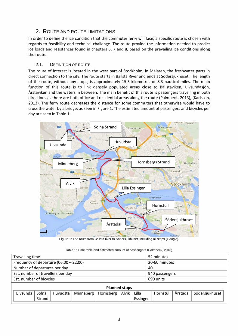
The route of interest is located in the west part of Stockholm, in Mälaren, the freshwater parts in direct connection to the city. The route starts in Bällsta River and ends at Södersjukhuset. The length of the route, without any stops, is approximately 15.3 kilometres or 8.3 nautical miles. The main function of this route is to link densely populated areas close to Bällstaviken, Ulvsundasjön, Årstaviken and the waters in between. The main benefit of this route is passengers travelling in both directions as there are both office and residential areas along the route (Palmbeck, 2013), (Karlsson, 2013). The ferry route decreases the distance for some commuters that otherwise would have to cross the water by a bridge, as seen in Figure 1. The estimated amount of passengers and bicycles per day are seen in Table 1.
Figure 1: The route from Bällsta river to Södersjukhuset, including all stops (Google).
Table 1: Time table and estimated amount of passengers (Palmbeck, 2013).
Travelling time 52 minutes
Frequency of departure (06.00 – 22.00) 20-60 minutes
Number of departures per day 40
Est. number of travellers per day 940 passengers
Est. number of bicycles 690 units
Planned stops
Ulvsunda Solna Strand
Huvudsta Minneberg Hornsberg Alvik Lilla Essingen
Hornstull Årstadal Södersjukhuset
Huvudsta
Södersjukhuset
Hornstull
Lilla Essingen
Minneberg
Solna Strand
Ulvsunda
Hornsbergs Strand
Alvik
Årstadal

4
2.2. DIMENSIONING FACTORS
External factors, who are rout dependant, will have a direct effect on the ship capacity. The factors having the largest impact to the list of criterions working as a foundation for the hull structure design are mentioned below.
2.2.1. Passenger demands
The ferry will be dimensioned to carry 150 passengers and 30% of them are estimated to bring their bicycles on board (Palmbeck, 2013). The number of passengers that the ferry can carry is slightly over dimensioned but as there is an unpredictable “popularity factor” for commuting with ferry, the number of passenger can be expected to increase (Karlsson, 2013), (Malmsten, 2014). The current plans involve side-to docking for the ferries to quicker load and unload passengers (Malmsten, 2014), (Rindeskär, 2014). The ferry developed in the further investigations will be based on these passenger requirements.
2.2.2. Speed
The time schedule (see Table 1) is based on a cruising speed of 12 knots. The limit is set by “experience” and is based on the speed limit in brash ice, which occurs in an ice channel winter time (Rindeskär, 2014), (Malmsten, 2014). A large part of the waters in central Stockholm also have a speed restriction of 12 knots. When breaking ice the speed of an ice breaking vessel is usually limited to approximately 5 knots. The maximum speed of the ferries is estimated to be around 14 knots. These values are the traditional speed limits based on empirical data and experience. The hull concept of the ferry can then be analysed more thoroughly.
2.2.3. Operational profile
The average operational profile for the vessel is 20 % running in brash ice channels, 2 % icebreaking and 78 % open water. This profile is based on weather data (SMHI, 2014) for the Stockholm region and ice growth models presented in 6.2
2.3. LIMITATIONS OF INVESTIGATION
Information that affects the details of the route but does not have an effect on the structural design of the ship hull, such as accessibility and bunkering, is not taken into account in this investigation.

5
3. MAIN PARTICULARS AND HULL PERFORMANCE This chapter contains information about the ferry in question. The level of detail presented here has to be put in perspective to the main aim of the thesis work. Numerical values are approximate and relevant simplifying assumptions concerning the general arrangement are defined and motivated. Principal layout and arrangement of main particulars are illustrated in the attached figures. The vessels main particulars are necessary to investigate hull resistances according to DNV rules, chapters 4.4 and 5, and the analytical/semi-empirical models in chapter 7.
3.1. MAIN PARTICULARS
The capacity demand and operational profile which is given in chapter 2.2 works as input when defining the main particulars of the vessel. Hull geometry, consistent with given data, is then produced and used to investigate the hydrostatic stability and open water resistance. Figure 2 below shows the starboard side of the ship and the main particulars for the given vessel are displayed in Table 2.
Figure 2: Side view of vessel.
Table 2: Main particulars for given vessel.
LOA 30 m
Lwl 27 m
DMLD 3.7 m
TDES 1.5 m
BWL 7.2 m
BMLD 7.8 m
DispMLD 115 ton
Main engine 2xVolvo Penta D13 450 (Volvo Penta, 2013)
Power 2x330 kW
Propulsion 2xAzimuth thrusters 1.1m diameter (Rolls Royce, 2014)
Bow thruster 50 kW electric bow thruster (Jastram manuevring competence, 2014)
Auxiliary generator 77 kW (Volvo Penta, 2013)
Nominal capacity 150 passengers
Maximum capacity 278 passengers
Seated 106 passengers
Standing 44 passengers
Bicycles/strollers 30 units
3.2. PASSENGER DECK
The ferry has a rated capacity for 150 passengers. The capacity also allows for 20% of the passengers to bring bicycles or strollers onboard. Boarding is done on either side in the aft or front through sliding doors, enabling direct access to the passenger compartment. The small foredeck in the bow is not to be used by commuters. Areas for bicycle storage are located in the most aft part of the

6
passenger compartment, and in the front part of the ship behind the half circle shaped high bench. Seats are mounted in pairs of two or three and mounted to passenger deck by bolting or similar. Rearrangement of seat configuration is enabled through a modular seat solution. Passenger deck is equipped with one lavatory located in front of the aft port embarking door. It is supposed to be designed according to SJÖFS 2004:25, guaranteeing accessibility for people in wheelchairs and people with children in strollers (Sjöfartsverket, 2010). Illustrations are provided in Figure 2 and Figure 3.
Figure 3: Illustrative top view of passenger deck for given vessel.
Passenger deck layout is focused on maximizing capacity and comfort for travellers, independent of season. A wide isle centered along the length of the deck enables passengers to pass each other, carrying baggage or leading strollers or bicycles. Wide open areas in direct connection to the doors simplify embarking and disembarking. The half circle shaped high bench in front of the forward bicycle area can hold ten commuters, providing them with an enjoyable view.
3.3. LOWER DECK ARRANGEMENTS
The lower deck of the ship is divided into six compartments which are visible in Figure 2. From the bow to the aft, these are named and provided with the following functions as seen below.
3.3.1. Collision void
The void is left empty.
3.3.2. Bow thruster room
Holding the machinery and associated systems and tooling for the bow thruster. The fore part of this void also holds two ballast tanks which are placed on either side of the vessel, each with a capacity of approximately 2.5 m3.
3.3.3. Main engine room
Holding the two main engines and associated systems. Main fuel tanks are also located in this compartment.
3.3.4. Auxiliary engine room
Holds the auxiliary engines, bilge pumps, service pumps and associated systems.
3.3.5. Storage room
Holding tools and equipment used for maintenance, as well as the two aft ballast tanks on either side, each with a volume of 3.6 m3. This room can also be used as dressing room for the staff.

7
3.3.6. Propulsion room
This room holds the steering equipment and systems for the electric azimuth propulsion.
3.4. WATERTIGHT COMPARTMENTS
Watertight compartments on lower deck are consistent with the compartment division. Longitudinal positioning and detailed measurements for further investigation of these compartments can be found in Table 3.
Table 3: Watertight compartments
Compartment name Aft position
[m from transom] Forward position [m from transom]
Collision void Bow thruster room Main engine room Auxiliary engine room Storage room Propulsion room
26.8 21.5 16.1 10.0 6.9 0
29.6 26.8 21.5 16.1 10.0 6.9
3.5. PASSENGER AND CARGO CAPACITY
Width of passenger compartment is set to 6.4 meters, equal to the width of six sitting passengers, four standing passengers and the estimated width of one bicycle. This is assumed to be a sufficient width for the passenger compartment, resulting in an isle width of 3 meters. Estimated width of embarking ramps and passenger doors is set to 1.6 meters. Detailed measurements used for estimation of area demand concerning passenger deck are defined in Table 4.
Table 4: Detailed measurements for estimation of passenger deck area.
Unit Width [m] Length [m] Weight [kg]
Standing passenger 0.6 0.6 75
Sitting passenger 0.6 0.8 75
Bicycle 0.4 1.7 12
Seat 0.6 0.6 30
8
4. HULL FORM AND FEATURES The two main features governing the design of this hull form is functionality and reliability. Another main area of interest is to define certain hull features that might contribute to a decreased operational resistance, which in turn results in decreased overall operational costs. An ice breaking hull is often characterized by a rounded stem, sloping sides and a short mid ship body defined by a constant transverse sectional shape, all to improve maneuverability in icy conditions. The ice slides in under the vessel and breaks, often without creating a noticeable change in the icebreakers trim. These hull features does however result in poor hydrodynamic efficiency and makes the vessel susceptible to slamming loads. Operation in open waters on the other hand, is favored by a bow shape characterized by a sharper stem with a greater stem angle, a longer parallel mid ship section and straight sides. It is hereby understood that the ships operational profile and regional location is of uttermost importance when choosing design features for the hull with the aim to minimize resistance. The operational profile of the ship is explained in 2.2. Main effort in the evaluation concerning resistance minimizing hull features is hereby focused on the bow, from the stem reaching back to the point where the hull sectional area becomes constant. This is mainly because the bow shape has the largest impact on the operational resistance, but also because it is thoroughly processed in the rules as well as in the direct calculations. DNV rules are coping with ice handling abilities in a way that secures the hull structure from being insufficiently strengthened. The detailed shape of the hull does however not affect the ice pressures for ice class ICE-1C, which the hull is designed for. There is no connection between certain hull features and ice loads given for this particular ice class. Thus no benefits would come from changing the hull shape with the aim to lower ice loads on the given hull structure. Brash ice resistance does however change with varying bow shape according to the rules (Det Norske Veritas, DNV service documents). The rule based expressions for ice loads and brash ice resistance is explained further in 5.3 and 5.5. Direct calculations for certain hull shapes on the other hand, points toward that certain hull features contribute to dramatically decreased ice loads, thus leading to a more accurate estimation of the loads which the hull is exposed to. The connection between brash ice resistance and ice loads which the hull is exposed to is explained further in 5.3 and 5.5.
4.1. HULL SHAPE
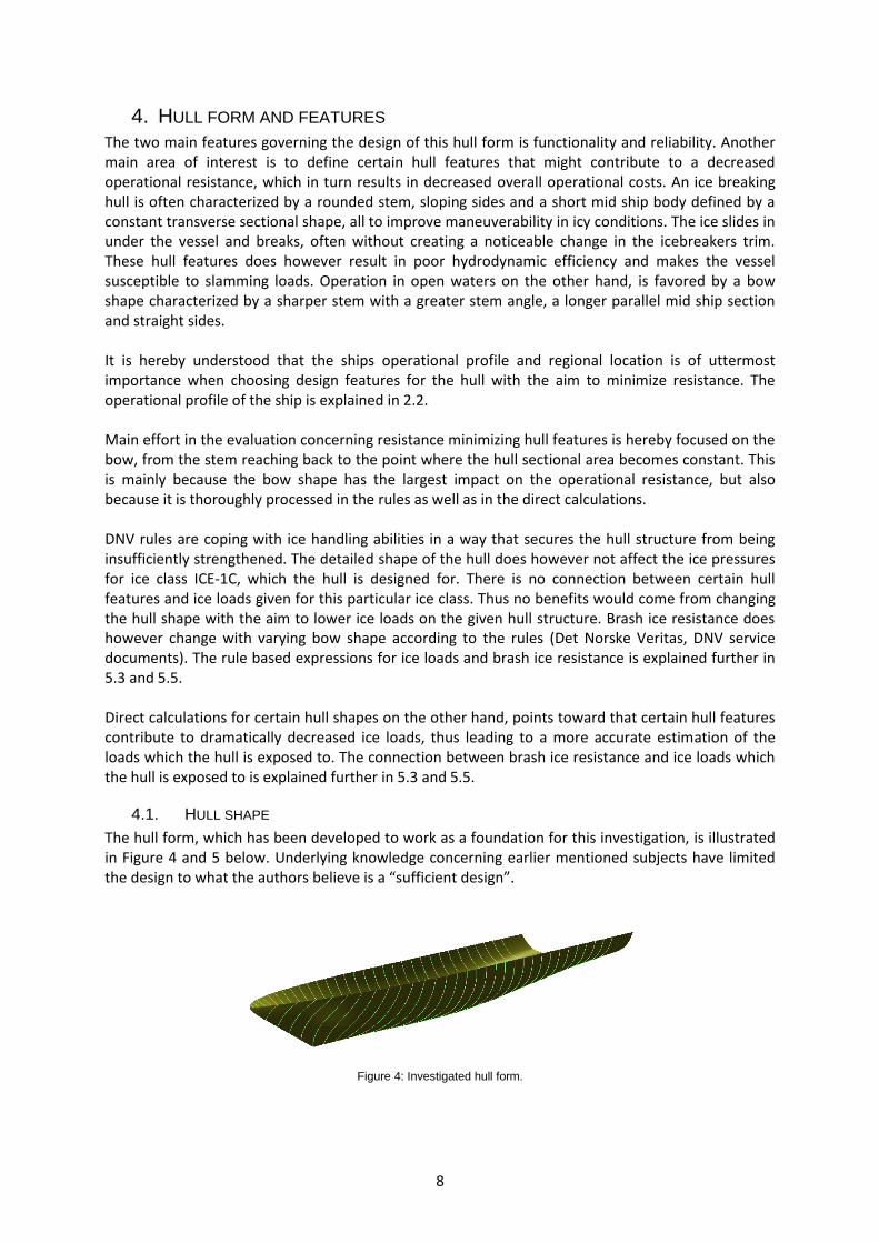
The hull form, which has been developed to work as a foundation for this investigation, is illustrated in Figure 4 and 5 below. Underlying knowledge concerning earlier mentioned subjects have limited the design to what the authors believe is a “sufficient design”.
Figure 4: Investigated hull form.
9
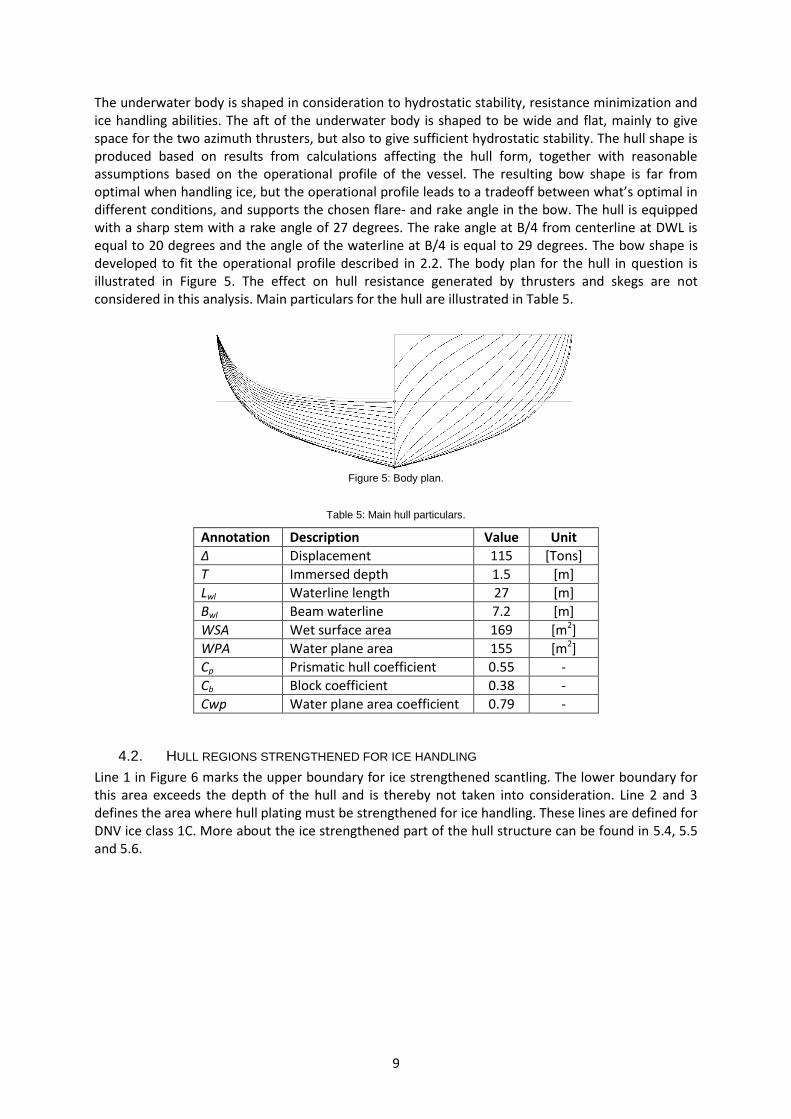
The underwater body is shaped in consideration to hydrostatic stability, resistance minimization and ice handling abilities. The aft of the underwater body is shaped to be wide and flat, mainly to give space for the two azimuth thrusters, but also to give sufficient hydrostatic stability. The hull shape is produced based on results from calculations affecting the hull form, together with reasonable assumptions based on the operational profile of the vessel. The resulting bow shape is far from optimal when handling ice, but the operational profile leads to a tradeoff between what’s optimal in different conditions, and supports the chosen flare- and rake angle in the bow. The hull is equipped with a sharp stem with a rake angle of 27 degrees. The rake angle at B/4 from centerline at DWL is equal to 20 degrees and the angle of the waterline at B/4 is equal to 29 degrees. The bow shape is developed to fit the operational profile described in 2.2. The body plan for the hull in question is illustrated in Figure 5. The effect on hull resistance generated by thrusters and skegs are not considered in this analysis. Main particulars for the hull are illustrated in Table 5.
Figure 5: Body plan.
Table 5: Main hull particulars.
Annotation Description Value Unit
Δ Displacement 115 [Tons]
T Immersed depth 1.5 [m]
Lwl Waterline length 27 [m]
Bwl Beam waterline 7.2 [m]
WSA Wet surface area 169 [m2]
WPA Water plane area 155 [m2]
Cp Prismatic hull coefficient 0.55 -
Cb Block coefficient 0.38 -
Cwp Water plane area coefficient 0.79 -
4.2. HULL REGIONS STRENGTHENED FOR ICE HANDLING
Line 1 in Figure 6 marks the upper boundary for ice strengthened scantling. The lower boundary for this area exceeds the depth of the hull and is thereby not taken into consideration. Line 2 and 3 defines the area where hull plating must be strengthened for ice handling. These lines are defined for DNV ice class 1C. More about the ice strengthened part of the hull structure can be found in 5.4, 5.5 and 5.6.

10
Figure 6: Ice strengthened regions.
4.3. STABILITY ANALYSIS
A full hydrostatic stability analysis falls outside the aim of this report and is thus not investigated here. Main focus for this analysis is to investigate whether the transversal hydrostatic stability is sufficient enough for different loading conditions. It provides vital information about the vessels capability of handling the capacity demands. An estimation of the weights of vital parts contributing to the complete displacement and stability works as a foundation for the load cases which are being investigated further in this chapter.
4.3.1. Estimation of weight and center of gravity for design load scenario
Table 6 below shows the estimation of center of gravity according to the design load scenario; nominal capacity load and full ballast tanks. The weights of different parts in Table 6 are approximated using different methods. Weights of structural components are estimated with the help of earlier knowledge in combination with reasonable assumptions. Weights of defined components, for example bow thruster, main engines, auxiliary engines and propulsion systems are all based on detailed product descriptions often used for ferries of this size.
Table 6: Estimation of weight and center of gravity.
Weight estimation
[tons] TCG
[x-direction] LCG
[y-direction] VCG
[z-direction]
Bridge 5 0 21.1 6.5
Passenger compartment 17.7 0 11.6 4.7
Passenger cargo 12 0 9.8 4
Main deck 15 0 15.5 3
Bow thruster system 0.6 0 25.4 1.5
Main engines 2x1.8 0 19.7 1.5
Auxiliary engine 1 0 13.7 1.5
Propulsion system 2x1.5 0 3.6 0.5
Hull structure 40 0 17.1 1
Other machinery equipment and systems
0.9 0 15.5 1
Fluids 3.4 0 15.5 0.5
Forward ballast tanks 2x2.5 0 25.1 0.5
Aft ballast tanks 2x3.6 0 8.9 0.5
Total 115 tons 0 ~15 m ~2.3 m
The hydrostatic stability is investigated for two different load cases which are defined in Table 7 below. The varying number of passengers and their location are estimated to a point load in each

11
load case, fixed in the ships reference system, one meter above passenger deck. This implies that the effect from the free surface moment induced by the moving mass of the passengers in large heeling angles is excluded from the analysis. The shape of the underwater body varies with changing heel, leading to a shift in LCB, which in turn induces a change in trim. The weight contribution from bicycles is not considered in any of the following load cases. The two load cases are investigated for stability criteria´s according to SJÖFS 2006:1 (Sjöfartsverket, 2006) and displayed as seen in Table 8. Sufficient hydrostatic stability in both bad cases point toward the hull shape in question fulfilling basic stability demands. This implies that it is applicable as a sample ship, acting as a foundation for further investigations.
Table 7: Hydrostatic stability load case variation.
Case number Number of passengers Total passenger weight [tons]
Transversal center of gravity [m]
Ballast
Design case 150 12 0 Full
Load case 1 150 12 1.5 Empty
4.3.1.1. Large angle stability investigation for design case
This condition is considered to be the normal condition in which the ship will operate during icy periods. Ballast tanks are full to lower the position of thrusters in the water, thus increasing maneuverability. This also induces a lowered CG.
Figure 7: GZ curve for evenly distributed design load and full ballast tanks.
Transversal center of gravity is zero since the passengers are considered to be evenly distributed over the deck. Vertical center of gravity is equal to approximately 2.3 meters above baseline. Longitudinal center of gravity is equal to 15.6 meters from the transom.
4.3.1.2. Large angle stability investigation for load case 1
This load case is considered the most extreme load scenario with nominal capacity utilization. 150 passengers shifted to port side. Transversal center of passenger load is estimated to 1.5 meters from the centerline. TCG increases to 0.178 meters from centerline. Ballast tanks are empty, thus resulting in a VCG equal to approximately 2.5 meters measured from baseline. LCG is still 15.6 meters.

12
Figure 8: Maximum heel induced by shifted nominal capacity and empty ballast tanks.
Figure 9: GZ-curve for unevenly distributed design load and empty ballast tanks.
Table 8: Criteria fulfilment for design load.
Criteria Design case Load case 1
1 OK OK 2 3 4 5 6
OK OK OK OK OK
OK OK OK OK OK

13
4.4. OPEN WATER RESISTANCE ESTIMATION
Different resistance prediction methods use a wide range of algorithms to estimate the resistance of a hull in open water. Every method is suitable for specific hull categories and thus some being more applicable than others in this particular case. Below follows a short description together with results from the applied prediction method. The propulsion efficiency is set to 100%, generating results which are correlated with the traction power needed to pull the vessel.
4.4.1. Slender Body Method
This is an analytical method that predicts the wave resistance of a port/starboard symmetrical monohull. Assumptions are made that the vessel has a slender shape, meaning high length-beam ratio and slenderness ratio (length-displacement ratio). Accurate results are gained for slenderness ratio between approximately 5.0 and 6.0. The minimum slenderness ratio for which the method is applicable is reduced if the length Froude number is reduced. Very high slenderness ratio has been found to generate reasonable results for Froude numbers up to 1.0. The method works equally well for round bilge hulls as for chine hull forms and deals automatically with transom sterns by adding a virtual attachment in the aft aligned with the bottom surface (Formsys, 2014) as illustrated in Figure 10.
Figure 10: Hull discretization with and without virtual appendage (Couser, Wellicome, & Molland, 1998)
The vessel in question has a slenderness ratio of approximately 6.2. This is however not a problem, since the length Froude number is below 0.4 at a speed of 12 knots. The slender body method is hereby assumed to give reasonable estimated values for needed tractive power in the complete speed interval. Tractive power estimation as function of speed or Froude length number is illustrated in Figure 11.
Figure 11: Tractive power as function of hull speed.

14
It can be seen that the tractive power estimation increases fast with increasing speed. Resistance seems to increase exponentially up to approximately 12.5 knots. The power estimation for speeds above 12.5 knots falls outside the operational profile and are thus considered irrelevant. About 550 kW is needed for 12 knots according to this method. This power is however not equal to the installed engine power, since the propulsion efficiency used in the performed calculations is set to 100%.
4.5. BRASH ICE RESISTANCE
The nature of rule based brash ice resistance estimation is presented in detail in 5.3.1. This estimation is as explained in 5.3.1 however only valid for a speed equal to 5 knots. Brash ice thickness in the channel is, according to the DNV rules, set to 0.6 meters for the chosen ice class 1C. It is clear from this method that a ship of this size and shape, by applying the defined angles and main particulars of the given hull, reaches a design brash ice resistance around 30 kN (5.3.1). This results in an approximated minimum engine output requirement of 220 kW, which is well within the limits of what is accounted for concerning propulsive power. It is however also clear that this engine output falls outside the validity range of the rule based brash ice resistance calculations defined in 5.3.4, which clearly is a problem when trying to construct the vessel according to the DNV rules. Required service speed is also preventing the calculations from generating sensible results, since the DNV based calculations are tuned for a speed of 5 knots. Brash ice resistance estimation based on DNV rules might therefore be far from reality, since the vessel is expected to operate in 12 knots in these conditions. This implies that the resistance estimation for this operational condition might be heavily underestimated, making it a subject for further investigation.
4.6. ICE BREAKING RESISTANCE
The DNV rules for dimensioning ice breaking resistance is usually applied for ice class 1A*. Other ice classes are allowed to exclude the resistance contribution due to a consolidated layer of brash ice in an ice channel. Total resistance at a speed of 5 knots in a brash ice channel with a consolidated layer of ice on top is, according to chapter 5.3.2 estimated to approximately 48 kN for this particular vessel. Minimum engine output requirement is given by chapter 5.3.3 and is equal to approximately 392 kW, which again is within the technical limits for the chosen engine arrangement, but outside the validity range of minimum engine power output given in 5.3.4.
4.7. DISCUSSION
The operational profile defined in 2.2 points toward the importance of the ship being able to follow the timetable all year around. Breaking ice is considered an exceptional operational condition, meaning that the demand for speed according the operational profile is left aside. An assumption that the vessel should be able to make a speed of 5 knots in these conditions is however made. This is based on the nature of DNV resistance estimation rules which are limited to a design speed of 5 knots. Values for required engine power output calculated above can be used as a foundation in combination with the operational profile to revise the engine arrangement and choose machinery optimal for this vessel. This revision is however left aside since it is considered too far from the main goal of the thesis. The hull shape has been developed through an iterative process involving open water resistance and hydrostatic stability calculations, while in the same time controlling main deck measurements, displacement and bow shape angles. This work has been performed using the hull shape development tool Maxsurf (Formsys, 2014).

15
The first design loop in the iterative development process is complete. Main parameters stated here are recurrent in the overall work and used as a foundation for the rest of the analytical conclusions in this report. Hydrostatic stability for this particular vessel is a subject for revision, which ultimately might lead to a change in the main parameters of the vessel. Effective methods for achieving a sufficient hydrostatic stability are for example to investigate the possibility of lowering center of gravity by altering the superstructure, or changing the shape of the underwater body. Reconfiguration of watertight bulkheads to increase ballast tank capacity might also be a relevant subject for further investigation. The hydrostatic stability analysis has to be refined to achieve sensible results for the different load cases. Free surface moments induced by partially filled tanks are one obvious point for refinement which can be crucial for the overall stability. This is however left for future design loops in the development process. The ice thickness which is applied when designing vessels for a particular ice class does not govern the operability of the ship alone. This particular vessel is for example according to its ice class, supposed to be able to make a speed of 5 knots in 0.6 meters of brash ice. Continuously operating the vessel in these conditions will increase the risk of mayor damage to propulsion systems and appendages. Further studies are therefore needed to ensure sufficient overall strength in these systems as well.

16
5. ICE CLASS RULES This chapter treats rules obtained by the DNV classification society concerning design regulations for vessels less than 100 meters trafficking icy waters. Main focus is aimed toward describing the design procedure of the hull structure. Specific decisions are made in the process to limit the investigation to the forward part of the hull and main particulars defined in chapter 3 are used as input values for the calculations. Results generated in this part of the report are partly recurring in other parts of the report. DNV rules are commonly accepted as equivalent to the Finnish Swedish ice class rules. Parts of the DNV rules for classification of ships processed in this chapter are listed below.
Part 1 chapter 2: “Class notations”
Part 3 chapter 2: “Hull Structural Design, Ships with Length Less than 100 meters”
Part 5 chapter 1: “Ships for Navigation in Ice”
5.1. GUIDELINES FROM THE SWEDISH TRANSPORT AGENCY
A ship shall be designed and constructed so that the strength of the hull, closures, rigging and equipment provides adequate safety for all conditions in which the ship is intended to operate and for all damage conditions which the ship is designed to survive. Special attention should be given to the static stresses appearing in the structure induced by the most severe load condition, usually a combination between the maximum load and the most severe load distribution. Special attention should also be taken to the dynamic stresses that might occur as result of the usage according to the operational profile. Ships shall be constructed in accordance to a legislated framework issued by a recognized organisation such as DNV GL, Lloyd’s Register or the American Bureau of Sipping. The Swedish Transport Agency can allow direct calculations as foundation for new types of ships or new design concepts, for which there are no applicable set of rules. These calculations together with all assumptions made, shall be reported to the Swedish Transport Agency for analytic review and approval. The documentation which is reported shall support the ships structural standard which is relevant for its operational profile (Swedish Transport Agency, 2013).
5.2. USE OF CLASSIFICATION RULES IN ENCLOSED WATERS
A service area notation is always given ships with specific modifications to general arrangement, structural scantling or equipment. This notation is marked R, followed by a number or a letter according to Table 9 below
Table 9: Service area restrictions (Det Norske Veritas, 2014).
Service area notation Seasonal zones
Winter Summer Tropical
R0 250 No restrictions No restrictions
R1 100 200 300
R2 50 100 200
R3 20 50 100
R4 5 10 20
RE Enclosed waters
Relevant service area notation for investigated vessel is RE. This restriction limits operation to enclosed waters such as rivers or lakes, which is considered suitable given the operational profile presented in chapter 2.2. The service area restriction notation is used in the rule based design process to obtain relevant results for the given vessel (Det Norske Veritas, 2014). Following requirements in relevant sections of the rules are modified in relation to the choice of service area;

17
Design hull girder loads
Design pressures on shell, weather decks, superstructures and deckhouses
Anchoring and mooring equipment
Arrangement
Stability
5.3. RULE BASED RESISTANCE CALCULATION
Resistance of the ship in a channel with brash ice and a consolidated layer of ice is given in the rules according to
(5.1)
Factors C1 and C2 are usually only taken into account when designing for ice class ICE-1A*, which is equated to operation in consolidated ice. The operational profile defined in chapter 2.2 does however not exclude the vessel from operation in conditions resulting in breaking consolidated ice in a brash ice channel; hence these constants need to be included in the resistance estimation for this particular operational condition.
5.3.1. Brash ice resistance
As explained earlier, C1 and C2 are excluded for this operational condition. C3 , C4 and C5 are all empirical coefficients set to 845 kg/m2s2, 42 kg/m2s2 and 825 kg/s2. Coefficients C𝜇 and C𝜓 are dependent on the shape of the bow accordingly:
(5.2)
(5.3)
The minimum value of C𝜇 is set to 0.45. C𝜓 is equal to 0 if 𝜓 exceeds 45 . The rake of the bow (𝜑2) and the water entrance angle (α), at the waterline at B/4 from the centerline, are both defined in degrees and illustrated in Figure 12 below.
Figure 12: Definition of bow angles according to DNV rules.
3
2 2
1 2 3 4 5 2
wf
CH F M F PAR F
ALTR C C C C H H B C H C L H C
B L
20.15cos sin sinC
0.047 2.115C
18
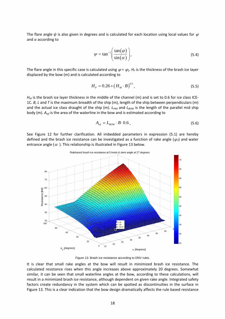
The flare angle 𝜓 is also given in degrees and is calculated for each location using local values for φ and 𝛼 according to
, (5.4)
The flare angle in this specific case is calculated using φ = φ2. HF is the thickness of the brash ice layer displaced by the bow (m) and is calculated according to
, (5.5)
HM is the brash ice layer thickness in the middle of the channel (m) and is set to 0.6 for ice class ICE-1C. B, L and T is the maximum breadth of the ship (m), length of the ship between perpendiculars (m) and the actual ice class draught of the ship (m). LPAR and LBOW is the length of the parallel mid ship body (m). Awf is the area of the waterline in the bow and is estimated according to
, (5.6)
See Figure 12 for further clarification. All imbedded parameters in expression (5.1) are hereby defined and the brash ice resistance can be investigated as a function of rake angle (φ2) and water entrance angle ( ). This relationship is illustrated in Figure 13 below.
Figure 13: Brash ice resistance according to DNV rules.
It is clear that small rake angles at the bow will result in minimized brash ice resistance. The calculated resistance rises when this angle increases above approximately 20 degrees. Somewhat similar, it can be seen that small waterline angles at the bow, according to these calculations, will result in a minimized brash ice resistance, although dependent on given rake angle. Integrated safety factors create redundancy in the system which can be spotted as discontinuities in the surface in Figure 13. This is a clear indication that the bow design dramatically affects the rule based resistance
1
tantan
sin
0.5
0.26F MH H B
0.6wf BOWA L B
1520
2530
3540
4550
55
0
20
40
60
80
100
20
30
40
50
60
70
80
[degrees]
X: 29
Y: 20
Z: 24.57
Rulebased brash ice resistance at 5 knots & stem angle at 27 degrees
2 [degrees]
Re
sis
tan
ce
[kN
]
25
30
35
40
45
50
55
60
65
70

19
for operation in brash ice. Worth mentioning is also that these calculations are based on a simplified version of reality and that they are restricted to a speed of 5 knots.
5.3.2. Ice breaking resistance
The last part of Equation (5.1) share some resemblance with Riska’s analytical expression for ice breaking resistance, presented in 7.3. Ice breaking resistance in a brash ice channel with a brash ice thickness in the middle of the channel equal to 0.6 meters is defined according to the DNV rules for ice class 1C by including the resistance contribution from C1 and C2 in expression (5.1) presented in 5.3.1 above. C1 is calculated according to
1 1 1 2 3 41 0.021
2 1
PARBOW BOW
BLC f f B f L f BL
T
B
(5.7)
The parameter f1 is set to 23 N/m2, f2 to 45.8 N/m, f3 to 14.7 N/m and f4 to 29 N/m2 (Det Norske Veritas, 2014). LBOW and LPAR is as explained earlier, equal to the length of the bow and midship section as illustrated in Figure 12. C2 is calculated using the following expression
2
2 1 1 2 31 0.063 1 1.2T B
C g g B gB L
(5.8)
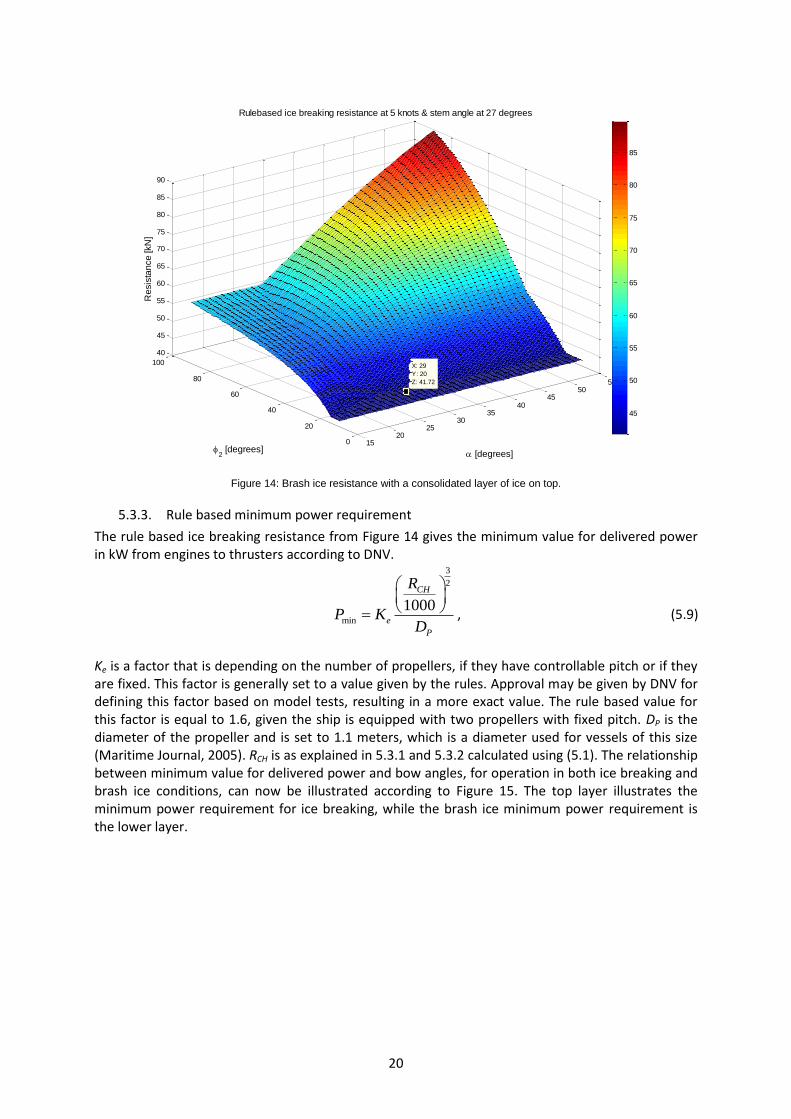
The value of g1 is set to 1530 N, g2 to 170 N/m and g3 to 400 N/m1.5 (Det Norske Veritas, 2014). These parameters are tuned by DNV and differ from the values obtained in Riska (Fel! Hittar inte referenskälla.). Figure 14 illustrates icebreaking resistance in relation to bow angles α and φ2 can now be visualized in the same way as with the brash ice resistance in Figure 13. Comparing these two figures clarifies that the different resistance estimations behave in the same way and that the rule based ice breaking resistance for the commuter ferry is about 17 kN higher than the brash ice resistance, only given the choice of stem angle.
20
Figure 14: Brash ice resistance with a consolidated layer of ice on top.
5.3.3. Rule based minimum power requirement
The rule based ice breaking resistance from Figure 14 gives the minimum value for delivered power in kW from engines to thrusters according to DNV.
, (5.9)
Ke is a factor that is depending on the number of propellers, if they have controllable pitch or if they are fixed. This factor is generally set to a value given by the rules. Approval may be given by DNV for defining this factor based on model tests, resulting in a more exact value. The rule based value for this factor is equal to 1.6, given the ship is equipped with two propellers with fixed pitch. DP is the diameter of the propeller and is set to 1.1 meters, which is a diameter used for vessels of this size (Maritime Journal, 2005). RCH is as explained in 5.3.1 and 5.3.2 calculated using (5.1). The relationship between minimum value for delivered power and bow angles, for operation in both ice breaking and brash ice conditions, can now be illustrated according to Figure 15. The top layer illustrates the minimum power requirement for ice breaking, while the brash ice minimum power requirement is the lower layer.
1520
2530
3540
4550
55
0
20
40
60
80
100
40
45
50
55
60
65
70
75
80
85
90
[degrees]
X: 29
Y: 20
Z: 41.72
Rulebased ice breaking resistance at 5 knots & stem angle at 27 degrees
2 [degrees]
Re
sis
tan
ce
[kN
]
45
50
55
60
65
70
75
80
85
3
2
min
1000CH
e
P
R
P KD

21
Figure 15: Minimum power requirement for according to DNV for operation in ice breaking and brash ice conditions as functions
of bow angles.
The equations for estimating resistance and power requirement, (5.1) and (5.9), is not used in the rules as foundation for calculating the design ice pressure presented in (5.12), as in the case with the direct calculations for brash ice and ice breaking resistances. There is no connection between the ice load estimation and the minimum power requirement estimation in the set of equations given by DNV. It can however still be used as a decision support for defining bow angles as well as engine arrangement, which are presented further in chapter 3. The chosen bow angles results in a minimum engine power output illustrated in the top layer in Figure 15.
5.3.4. Validity range
DNV design rules only give a viable result within certain intervals. The model is, for example, only valid when minimum required engine output (Pmin) exceeds 1000 kW. Bow angles for the vessel under investigation fulfill the validity criteria’s. All validity perimeters governing whether the model is applicable or not is presented further in Table 10.
Table 10: Parameter validity range.
Parameter Symbol Minimum Maximum Value Validity
Water entrance angle α 15 55 29 Valid
Stem angle φ1 25 90 27 Valid
Angle at B/4 φ2 10 90 20 Valid
Length over all L 65.0 250.0 27 Invalid
Beam B 11.0 40.0 7.8 Invalid
Draught T 4.0 15.0 1.5 Invalid
Length of bow/L LBOW/L 0.15 0.40 0.48 Invalid
Length of parallel midbody/L LPAR/L 0.25 0.75 0.10 Invalid
DP/T 0.45 0.75 0.73 Valid
Awf/(L∙B) 0.09 0.27 0.29 Invalid
Minimum power enginge output Pmin 1000 kW - 400 kW Invalid
1520
2530
3540
4550
55
0
20
40
60
80
100
0
200
400
600
800
1000
1200
1400
[degrees]
X: 29
Y: 20
Z: 177.2
X: 29
Y: 20
Z: 392
Rulebased resistance in icy conditions at 5 knots & stem angle at 27 degrees
2 [degrees]
Re
sis
tan
ce
[kW
]
200
300
400
500
600
700
800
900
1000
1100
1200

22
5.4. DEFINITION OF ICE BELT REGION
The DNV ice class regulations divide the hull into three major regions, bow, mid body and stern region, which are to be strengthened for ice loads (Figure 16). The bow region consists of three sub regions; upper bow ice belt, ice belt bow region and fore foot region.
Figure 16: Ice belt regions according to DNV.
Main focus for this work is the ice belt bow region, reaching from the stem to a line parallel to and 4 % of L aft of the forward borderline seen in Figure 16. This borderline is the forward borderline marking the forward end of the mid body where the waterlines run parallel to the centre line. The ice belt region does however not need to exceed 5 meters aft of the borderline for the chosen ice class (ICE-1C). Vertically, this region covers the sides from the Upper Ice Water Line (UIWL) down to the Lower Ice Water Line (LIWL). These waterlines can be broken lines and should be the envelopes of the highest and lowest waterline at which the ship is intended to operate in ice (Det Norske Veritas, 2014). The vertical extension of ice-strengthened areas on ship hulls is dependent on the choice of ice class. Type of structural member is also affecting the extent of this region. Rule based values for the vertical extension of this region for ice class ICE-1C is defined in Table 11.
Table 11: Vertical extension of ice belt plating and framing for ice class ICE-1C (Det Norske Veritas, 2014).
Structural member Region Above UIWL [m] Below LIWL [m]
Plating
Bow
0.4
0.70
Mid ship 0.60
Stern
Framing
Bow
1.0
1.6
Mid ship 1.3
Stern 1.0
5.4.1. Definition of hull region under investigation
Chosen area of the hull which is under investigation concerning sufficient hull scantling in terms of strength and minimum structural thicknesses is limited by the total span in which the immersed

23
depth can vary in combination with the values in Table 11, together with the chosen longitudinal boundaries. The stem of the ship is defining the forward boundary of the investigated area. Aft boundary is coinciding with the third watertight bulkhead from the bow which is forming the aft wall of the bow thruster room. The third bulkhead is located at approximately 70 % of the total ship length measured from the aft. The choice of region for further investigation is motivated by the fact that it is assumed to be exposed to the greatest ice pressure according to the rules. Other motivational factors acting as foundation for the choice of hull region under investigation is the validity of the corresponding analytical load model presented further on in chapter 8. Maximum vertical span of the ice belt region in the bow is 1.36 meters for plating and 2.86 meters for framing. Ship hull region under investigation is marked in red in Figure 17.
Figure 17: Investigated area subjected to ice loads.
5.5. CALCULATION OF PRESSURE LOADS
The investigation is focused on DNV’s local ice loads and local sea pressure loads acting on the side structure. Sea pressure loads on bottom structure given by the DNV rules are acting on a part of the hull located below the ice belt region, which in this case is located below the physical boundaries of the ferry hull. This is the single main reason to why no further investigation is performed for these pressures.
5.5.1. Side structure
Loads given in Table 12 are in general applicable on the side structure of ship hulls according to the DNV rules. This particular investigation is limited to p1 and p2 in Table 12, which are the sea pressure estimations in direct connection to the summer load waterline, acting on the investigated ice belt region (Det Norske Veritas, 2014).

24
Table 12: Design loads applicable on side structures (Det Norske Veritas, 2014).
Equation for p1 given in Table 12 is dependent on h0 found in Table 14 and the pdp is defined accordingly
(5.10)
Where
(5.11)
Factor y in equation (5.10) is the horizontal distance from center line to the load point (a minimum of B/4 meters), B is the greatest molded depth in meters measured at the summer load waterline, T is the mean molded summer draught in meters and z is the vertical distance from the baseline to the load point. The parameter ks in equation (5.11) is varying over the ship length according to Table 13. ks is varied linearly between specified areas defined in column three in Table 13. The change of ks along ship length is illustrated in Figure 18.
Table 13:Variation of ks over ship length.
ks
At aft perpendicular and aft
Between 0.2L and 0.7L from aft perpendicular
At forward perpendicular and forward
135 1.275
dp l
yp p T z
B
0.8 0.15l s W f
Vp k C k
L
2.53 B
B
CC
2
4.03 B
B
CC

25
Figure 18 Variation of the parameter ks over the length of the ship
The illustration of how ks varies over the ship length indicates that the greatest design load appears in the bow. Parameter kf is the smallest of T and the vertical distance from the waterline to the top of the ship side at considered transverse section. Factor CW is set to 0.0792 times the ship length. An attempt to deepen the understanding of how the sea pressure above and below the waterline in theory changes over the ship hull side according to DNV can be seen in Figure 19 below.
Figure 19: Design sea pressure on side structure.
It is hereby evident that the greatest sea pressure is given by p1, located at the bow in level with the baseline. Worth mentioning is the discontinuity in the surface seen in the Figure 19. It illustrates that the design pressure used above summer load waterline is limited to a minimum value based on the ship length. When comparing this pressure to the design pressure applied below the same line, one
0 5 10 15 20 25 300
2
4
6
8
10
12
Variation of ks over ship length
ks [
m]
Ship length measured from the aft [m]
0
5
10
15
20
25
30
0
0.5
1
1.5
2
2.5
3
-10
0
10
20
30
40
50
60
Longitudinal location on hull side from aft [m]
[Sea pressure onto hull side]
Vertical location on hull side from keel [m]
Pre
ssure
[kN
/m^2
]
0
10
20
30
40
50

26
can see that this pressure also should be restricted in the same manner. This empirical sea pressure formula has been tuned over time to handle nonlinear effects and was initially based on strip theory calculations (Det Norske Veritas, 2014).
5.5.2. Loads from operation in ice
The hull is, according to DNV rules and depending on relevant ice class, dimensioned for operation in sea conditions corresponding to an ice thickness not exceeding h0 (Table 14). The actual ice pressure acting somewhere on the ice belt region at an arbitrary point of time is considered to be acting on a surface with a height h equal to a fraction of the ice thickness. This is why the design height h is smaller than the level ice thickness h0. Values for these two parameters are dependent on ice class and are defined in Table 14 below (Det Norske Veritas, 2014).
Table 14: Values for h and h0 (Det Norske Veritas, 2014).
Ice Class h0 [m] h [m]
ICE-1A* ICE-1A ICE-1B ICE-1C
1.0 0.8 0.6 0.4
0.35 0.30 0.25 0.22
Dimensioning ice thickness is according to Table 14 limited to 0.4 meters for ice class ICE-1C. The selected ice class 1C corresponds well to current estimations of ice thickness in the region under investigation defined in 6.2.1. The design height h is partly used for defining thickness of the shell plating in the ice belt region.
Ice loads acting on the ice belt region of the hull differ over time and accurate measurements of these loads show that they are completely random, best simulated by a stochastic pattern of pressure peaks, which is described further in 8.2. General simplification of ice loads are being used in the DNV rules. Observations have shown that the load distribution on a frame might be higher than on the shell plating in the middle between the frames, illustrated as p in Figure 20. Assumptions have been made and the distribution of design ice pressure on the hull structure is defined as p according
to Figure 20.
Figure 20: Assumed ice pressure distribution on hull structure.
The design ice pressure is calculated accordingly
p = p
0×c
d×c
1×c
a (5.12)
Where p0 is the nominal ice pressure set to 5600 kN/m2, cd is a factor influenced by engine output and size, c1 is a factor that takes into account the probability that the design ice pressure will occur on a certain part of the hull for a specific ice class and ca is a factor which takes into account that the full length of the considered area will be under pressure at the same time (Det Norske Veritas, 2014).
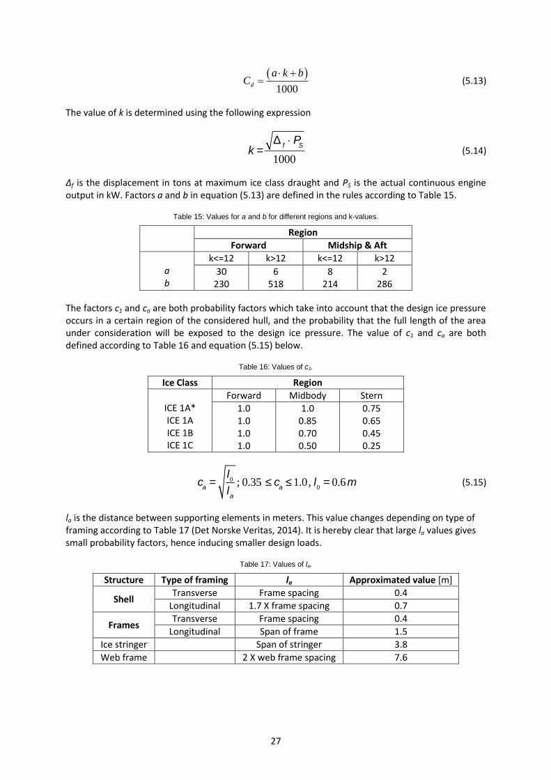
Cd is calculated accordingly
27
1000d
a k bC
(5.13)
The value of k is determined using the following expression
k =
Df×P
S
1000 (5.14)
Δf is the displacement in tons at maximum ice class draught and PS is the actual continuous engine output in kW. Factors a and b in equation (5.13) are defined in the rules according to Table 15.
Table 15: Values for a and b for different regions and k-values.
Region
Forward Midship & Aft
a b
k<=12 k>12 k<=12 k>12
30 230
6 518
8 214
2 286
The factors c1 and ca are both probability factors which take into account that the design ice pressure occurs in a certain region of the considered hull, and the probability that the full length of the area under consideration will be exposed to the design ice pressure. The value of c1 and ca are both defined according to Table 16 and equation (5.15) below.
Table 16: Values of c1.
Ice Class Region
ICE 1A* ICE 1A ICE 1B ICE 1C
Forward Midbody Stern
1.0 1.0 1.0 1.0
1.0 0.85 0.70 0.50
0.75 0.65 0.45 0.25
ca
=l0
la
; 0.35 £ ca
£1.0, l0
= 0.6m (5.15)
la is the distance between supporting elements in meters. This value changes depending on type of framing according to Table 17 (Det Norske Veritas, 2014). It is hereby clear that large la values gives small probability factors, hence inducing smaller design loads.
Table 17: Values of la.
Structure Type of framing la Approximated value [m]
Shell Transverse Frame spacing 0.4
Longitudinal 1.7 X frame spacing 0.7
Frames Transverse Frame spacing 0.4
Longitudinal Span of frame 1.5
Ice stringer Span of stringer 3.8
Web frame 2 X web frame spacing 7.6

28
5.5.3. Load comparison
A load comparison can hereby be performed to investigate the differences in design loads given by the rules. Estimated maximum design ice pressure onto the hull plating, located in the bow, reaches according to Figure 21 below a value of 1330 kPa for plates and frames. Maximum value for the ice stringer is approximately 530 kPa. The significantly lower design pressure for the ice stringer is due to the fact that the probability for the design ice pressure to act on the whole length of the stringer is smaller compared to the probability that it would act on a surface equal to the size of a plate.
Figure 21: Design ice pressure along the waterline.
The great discontinuity of the design ice pressure along the ship hull seen in Figure 21 is due to the nature of the DNV rule based ice pressure calculations, where safety factors are integrated into the equations. The great increase of design pressure in the front illustrates the effect from these safety factors in DNV:s systematic approach. The design load which will generate the ruling minimum plate thickness criteria is the DNV ice pressure design load.
5.6. CALCULATION OF PLATE THICKNESSES
Plate thicknesses in the hull structure are differing dependent on the size of the hull plate, where it is located and how the hull is constructed. Since the side structure is in focus, other parts are left out in this chapter. The investigation has been further limited to simply focus on the ship bow, reaching from the stem to approximately 70% of the overall length measured from the aft. The hull plates are assumed to be of rectangular shape with the side dimensions defined accordingly
0 5 10 15 20 25 300
200
400
600
800
1000
1200
1400Design Ice pressure
Longitudinal location measured from aft [m]
Pre
ssure
[kP
a]
Shell design pressure
Ice stringer design pressure

29
Figure 22: Stiffener span and stiffener spacing (Det Norske Veritas, 2014).
5.6.1. General plate thickness requirements
General plate thickness requirements are supposed to work as a minimum requirement in cases where local plate thickness requirements either result in insufficient plate thickness or are non-existing. Plate thickness for plating exposed to lateral pressure is, according to DNV rules for ships less than 100 meters, generally given by following expression:
treq,1
= 15.8 k
as p
s f1
+ tk (5.16)
The parameter tk is the corrosion thickness addition, s is the stiffener spacing in meters, p is the maximum lateral pressure in kPa, σ is the allowable local stress for the material and f1 is a material factor which is dependent on the material strength group according to Table 18.
Table 18: Value of f1.
ka in equation (5.16) is a correction factor concerning the aspect ratio of the plate field. It is calculated accordingly
2
1.1 0.25a
sk
l
(5.17)
The correction factor is limited to a maximum of 1.0 for s/l = 0.4 and a minimum of 0.72 for s/l = 1.0, which implies that the general thickness requirement in equation (5.16) reaches its maximum when the aspect ratio of stiffener span equal to 2.5 times the stiffener spacing. The thickness requirement presented in equation (5.16) does not necessarily have to be the dominating general thickness requirement. Another requirement based on strength is given by following expression:
Material strength group Value of f1
NV-NS NV-27 NV-32 NV-36 NV-40
1.00 1.08 1.28 1.39 1.47

30
treq,2
= t0+
k L
f1
+ tk (5.18)
Where t0 is the minimum plate thickness demand dependent on where the plate is located, k is a factor given in the DNV rules for each structural area (bottom, side or deck) and L is the length of the ship in meters (maximum 100).
5.6.2. Side structure
There are three main expressions governing the minimum thickness requirement for the plating of the side structure for this particular vessel. Expression (5.16) and (5.18) are adjusted when applied in different areas of the hull. This is becomes clear when investigating expressions for plate thickness requirement concerning side structure. Equation (5.16) then looks accordingly:
tside,req,1
= 15.8 k
as p
s+ t
k (5.19)
The load p is chosen from Table 12 depending on which load scenario the hull plating is investigated for. Focus is however aimed toward p1 and p2, as mentioned earlier. Equation (5.18) is adjusted in the same manner:
, ,2 5.0side req kt kL t (5.20)
Factor k is set to 0.04 for side plating up to 4.6 meters above summer load waterline. This value may be reduced by 0.01 for every 2.3 meters above this level and is limited to a minimum value of 0. The third plate thickness requirement is based on the estimated ice pressure which the hull side is exposed to. The orientation of the plate is affecting the thickness requirement, since it always is assumed to be stiffened along the longer side of it. Hence, this minimum thickness requirement differs depending on the structure being transversely or longitudinally stiffened. Following equation is used for transverse framing, where longitudinal plate side length is the shortest and equal to stiffener spacing
(5.21)
Factor s is the frame spacing in meters, pPL is 75% of the estimated design ice pressure illustrated in Figure 20, σF is the yield stress of the material, tc is the thickness increment of abrasion and corrosion, and f1 is a factor which is calculated accordingly
1 2
4.21.3
1.8
fh
s
(5.22)
Value of h is, as mentioned earlier, dependent on ice class and given in Table 14. The following equation is used for longitudinal framing, where lateral plate side length is the shortest and equal to stiffener spacing
longitu
2
dinal 21.1 PLc
F
pt s t
f
(5.23)
1 21.1 PLtransverse c
F
f pt s t

31
Factor f2 is calculated differently depending on the ratio h/s.
Table 19: Expressions for the factor f2 (Det Norske Veritas, 2014).
Interval Equation for f2
h/s ≤ 1
2
0.40.6
/f
h s
1 ≤ h/s < 1.8 2 1.4 0.4 /f h s
1 ≤ h/s < 3 2 0.35 0.183 /f h s
h/s > 3 2 0.9f
For the particular vessel in question, the ration h/s is equal to 0.55, hence the first expression for f2 in Table 19 is the one to be used. Two interesting comparisons can be made when taking these expressions into consideration. The first one is to investigate how these thickness requirements changes with varying frame spacing and span. This is illustrated in Figure 23.
Figure 23: Hull plate thickness requirement for ship bow.
Figure 23 consists of three surfaces, here defined from bottom to top. The double curved surface in the bottom is the thickness requirement for bottom plates exposed to lateral pressure given by equation (5.19) above. The second surface from the bottom, which is almost completely covered, is a horizontal plane. It is the minimum plate thickness requirement for side plates given by equation (5.20). The upper most surface is the plate thickness requirement for handling given design ice pressure loads. The axisymmetric discontinuity displayed is due to the fact that the requirement for how the structure is stiffened depends on the ratio between longitudinal and transversal propagation of the
0.10.2
0.30.4
0.50.6
0.70.8
0.91
0
0.2
0.4
0.6
0.8
1
0
5
10
15
20
25
30
Lateral propagation [m]
Shell plate thickness in relation to frame span and frame spacing
Longitudinal propagation [m]
Required t
hic
kness [
mm
]

32
plate sides. The shorter side of the hull plate is the one that governs relevant equation used to calculate the minimum plate thickness. The parameter s is set to this particular value, as explained earlier. This implies that changing dimensions also results in changing the way the structure is stiffened (longitudinally or transversally stiffened), hence the axisymmetric discontinuity in the top surface. It is hereby also clear that a transversally stiffened structure is preferred when minimizing the rule based plate thickness requirement for the side structure in the bow, since it allows for thinner hull plating.
5.7. HULL SCANTLING CALCULATIONS
Main focus for the calculations presented in this part is to illustrate how a hull scantling can be defined through knowledge of restricted geometrical dimensions, requirements given from design rules and basic solid mechanics. Specific focus is from here on guided toward the area of the hull that reaches from the stem to the third watertight bulkhead, from the baseline to the railing.
Figure 24: Hull part under investigation.
Two reasons are mainly governing the choice of area to be investigated. It is located within the maximum ice load region, which according to the rules is reaching from the stem to 70% of the ship length measured from the aft perpendicular. Secondly, it includes the longest watertight compartment, resulting in the longest girder span along given ice load region. Scantling optimized for this particular area is extended to cover the total investigated part of the hull, meaning that the scantling in compartment one and two counted from the stem, most likely will be unnecessarily strengthened. This is however not taken into consideration when dimensioning structural members. Span and spacing for frames and girders are set to approximated mean values based on the dimensions of this particular hull part and thus not changed for hull parts located in other compartments. Dimensioning requirements given in DNV rules are based on shear area and section modulus for all parts, except for bulkheads and plating where requirements are based on plate thicknesses. Shear area and section modulus for structural members are calculated according to equations (5.24) and (5.25).

33
Figure 25: Dimension definition for structural beams such as girders and stiffeners.
Shear area is marked with grey and illustrated in Figure 25 as
(t h t ) tshear plate web flange webA (5.24)
Section modulus varies over the cross section. Minimum section modulus is achieved along the top side of the flange due to the fact that it is positioned furthest away from the center of gravity for given cross section. It is calculated accordingly
max
yIZ
z (5.25)
Where Iy is the moment of inertia around y-axis and zmax is the maximum distance from center of gravity to top side of flange. Effective flange width (be) is needed for calculation of moment of inertia and is defined in the rules accordingly
eb C b (5.26)
Factor C is given by the rules and plotted in Figure 26.
Figure 26: Value of C.
Investigated members of the hull structure are considered to be exposed to a uniform pressure. This estimation simplifies the way of looking at the boundary condition of current members, since they
0 1 2 3 4 5 6 70
0.1
0.2
0.3
0.4
0.5
0.6
0.7
0.8
0.9
1
a/b
C
C - effective breadth coefficient
C(r<=3)
C(r=4)
C(r=5)
C(r>=6)
s
tweb
Wflange
tflange
Hweb
tplate

34
can be considered clamped in both ends. The value of a in a/b, making the x-axis in Figure 26, is the distance between the points of zero bending moment for given member. This value is according to the rules equal to 0.6 times the member span for members which can be considered clamped. The value of b is equal to the width of the plate field which the current structural member supports. The value of r is equal to the number of perpendicular members of lower hierarchy crossing the current member within given span. Hence, C for longitudinal girders are defined in Figure 26 by C (r≥6), while C for transverse framing is defined by C (r≤3). Figure 27 below visualizes effective flange width be for a T-beam connected to a plate.
Figure 27: Uniaxial stress for T-beam connected to plate.
5.7.1. Bulkheads
Bulkheads are as explained in 3.3 and 3.4, positioned to utilize the void below strength deck and to divide the ship into a number of watertight compartments. Plate thickness for this structure is governed by the thickness requirements given in part 3, chapter 2, section 8 concerning bulkhead structures. A minimum design thickness of about 8 mm is given by these equations. The thickness is however set to the same thickness as the ice strengthened plating, equal to 15 mm, which is a more conservative value.
5.7.2. Longitudinal girders
There is one longitudinal girder located at the datum waterline (marked in red in Figure 24) and two girders placed on the upper and lower boundary of the ice strengthened plating (marked in blue in Figure 24). The red girder is dimensioned according to requirements concerning longitudinal girders inside the ice belt, while the blue girders are dimensioned according to requirements concerning longitudinal girders outside the ice belt. Table 21 and Table 22 include dimensioning values that are chosen respectively.
Table 20: Approximated required and chosen section modulus and shear area for girders.
Required section modulus Z [cm3]
Chosen Z value [cm3]
Required shear area As [cm2]
Chosen shear area As [cm2]
Girder inside ice belt 941 951 33 41
Girders outside ice belt 567 667 21 28
Table 21: Chosen dimensions for longitudinal girders [mm].
tflange wflange tweb hweb tplate beffective
Girder inside ice belt 13 180 13 300 15 1260
Girders outside ice belt 15 180 13 200 15 1260

35
5.7.3. Framing
The hull is transversally stiffened with the frame spacing set to the static value 0.4 meters. Spacing between bulkhead and closest frame can vary depending on location of current members.
Table 22: Approximated required and chosen section modulus and shear area for transverse framing.
Required section modulus Z [cm3]
Chosen Z value [cm3]
Required shear area As [cm2]
Chosen shear area As [cm2]
Transverse framing 117 179 5.2 17.6
Table 23:Chosen dimensions for transverse framing [mm].
tflange wflange tweb hweb tplate beffective
Transverse framing 13 120 13 120 13 160
5.7.4. Plating
The hull plating is strengthened according to the DNV rules for ice strengthened hull plating, together with rules for general hull structural design. The area which is strengthened for handling ice reaches along the total length of the ice belt region, from stem to aft, and is extended vertically from 0.6 meters below lower ice waterline (LIWL) to 0.4 meters above upper ice waterline (UIWL). Plate thickness requirement for given scantling and ice pressure load is equal to approximately 14.8 mm. The hull plate in this region is rounded off and set to 15 mm. Relationship between hull plate dimensions, forces and how the hull is structured is illustrated in Figure 24 above.
5.7.5. Choice of material
The choice of material is governed by the DNV rules which defines the minimum quality grade for certain categories of structural members. Minimum material grade for shell strakes in way of the ice strengthened area for plating must at least be of grade B/AH. This allows for normal strength steel (NS), as well as for high strength steel (HS) to be used. Hull material strength groups which are provided by the DNV rules to be used in the calculations are given accordingly.
Table 24: Material strength groups.
Denotation Strength group Minimum Yield point value
NS HS HS HS HS
NV-NS NV-27 NV-32 NV-36 NV-40
235 265 315 355 390
One high strength steel type often used for construction of ship hulls today are NV-36. It is considered to be a material that is easy to work with and in the same time offering material properties allowing for a lighter hull construction compared to steel type with lower yield strength. The disadvantage of this HS steel is however its inability to handle cyclic loads due to the fact that higher strength materials allow for a thinner construction, which makes it more sensitive to fatigue cracks. Material chosen for this specific construction belongs to the NS strength group. This is negative from an operating cost point of view since it results in a heavier construction. The structure does however become less susceptible to fatigue, which is coherent with the operational profile that prioritizes reliability and safety. This choice of material sets the value for f1 to 1, which is defined in Table 18 and used in equation (5.16).

36
5.8. DISCUSSION & CONCLUSION
The first design loop concerning local hull structure in the bow is completed and results from calculations are used as foundation for the finite element analysis presented in chapter 9. Defined local scantling presented here is sufficient in terms of local strength and handling of local ice loads and hydrodynamic loads according to the DNV rules. The designed structure is limited to defined members presented in this chapter. Simplifying calculations a bit, the design of load carrying structural members are limited to T-shaped profiles, which results in shear center and neutral axis coinciding over the centerline of each member. Dimensioning global- and internal load calculations are, as mentioned earlier, excluded from this work and might, when investigated for, result in the given structure being insufficiently strengthened. An optimization of the scantling dimensions by minimizing both shear area and section modulus for each structural member in the given scantling will result in a lower weight which is considered relevant for minimizing operational cost and thereby an important subject for future investigation. A total refinement of the model, for example concerning calculations to define dimensions for a keel- and stem structure and to study how the scantling can vary individually for each member given the varying local scantling measurements, need also to be investigated further. The bulkhead structure also needs to be defined in detail. The effect on hull structural strength induced by the bow thruster might not be possible to neglect and may have to be investigated. This chapter is only focusing on the first 30 percent of the hull lengthwise, and could be developed to cover the complete hull structure, which would give a better understanding of how the scantling is allowed to vary along the length of the hull according to DNV. The pressure formula has to be investigated further to ensure the reliability of the results, since they differ significantly from the analytical equivalence presented in 8.3.2. This can be performed using a statistical approach to the problem, investigating the design ice pressures for ships of varying size, providing a better insight into how the pressure varies for different vessels.

37
6. ICE The design loads on an ice-going and ice-breaking ferry are dimensioning for the structure. The most severe load case when operating in ice conditions are the criteria to which the hull structure is designed. There are no rules1 adapted for designing smaller vessels such as a commuter ferry. The classification of ice going vessels is focused on ice breakers and merchant ships as well as offshore structures. This section aims at deriving relevant design loads for a smaller ferry (150 pax) as well as ice-going and icebreaking resistances. Icebreaking and ice-going vessels performance is in general based on average ice conditions (Martio, 2007). Ice can form in many shapes and the properties of the ice vary with temperature of water and air, salinity (for sea ice), weather, currents and more. Some of the most likely shapes of ice and the properties of ice are discussed in this section.
6.1.1. Level ice
Level ice is a layer of sea or lake ice without any deformations. Level ice forms when the water freezes during calm conditions. The level ice can later be deformed by the movements of the ice. Multi-year level sea is subjected to brine drainage thus reducing the salinity of the ice.
6.1.2. Ice floes Ice floes form when a solid ice sheet is cracked. The floes are typically larger than 20 m across but sometimes as big as several kilometers across.
Figure 28: Ice floes on open water and in a channel (SMHI, 2011a).
6.1.3. Ice ridges
Ridges in the ice are formed by compression when two ice sheets or large floes are driven towards each other. Shear is another formation mode of ridges and happens when large sheets of ice slide along each other and the edges are sheared off and the debris form ridges when re-freezing. A form of barrier can form on the side of a channel, causing the same problem as an ice ridge.
Figure 29: Ice ridge (SMHI, 2011a).
1 ABS, DNV GL and FSICR does not have any applicable ice rules for ferries of this size.

38
6.1.4. Brash ice
Brash ice is found in ship channels and is made by the ice breaking vessels making the channel and the ice-going vessels travelling in the channel. Initially the ice pieces have sharp edges and vary in size between 0.02 m and 2 m in diameter. With time they are rounded and the size is more even, and usually the pieces become fairly small. The brash layer can become so thick that ice going and ice breaking vessels will be severely limited in their movement and a new channel has to be made. The brash ice layers thickness depends on several parameters such as temperature of air and water, number of passaging ships and the movement of the level ice. (Mellor, 1980)
Figure 30: Brash ice channel in Stockholm. From (NordicPhotos, 2011)
Eventually the brash ice layer will become so thick that the resistance is higher than the ship can overpower and a new channel has to be broken. A Great Lakes bulk carrier in Canada is near its limit of movement when the brash thickness in a wide channel reaches 10 % of the vessels beam (Mellor, 1980). A consolidated layer can form rapidly during cold weather causing regular ferry traffic to run the channels once or twice during the night to keep them open (Rindeskär, 2014).
Figure 31: Brash ice in channel.
The thickness of the brash layer is difficult to predict in the case of the ferry traffic as most brash ice models are based on commercial traffic in sea water ice. However, a minimum brash ice thickness for different ice classed vessels is stated in the Finnish-Swedish Ice Class Rules and DNV ice class rules. The thickness of the brash ice layer in the middle of the channel that different classes needs to maintain a minimum speed of five knots in is 1m for 1A, 0.8 m for 1B and 0.6 m for 1C (TRAFI, 2011).

39
6.1.5. Pancake ice
Pancake ice is a form of ice that consists of rounded pieces of ice with a diameter ranging from 0.3 m to 3 m. The thickness is usually no more than 10 cm. The pancake ice forms on waters covered to some degree by ice slush or frazil ice. In these conditions there are such movements of the water that a level ice sheet cannot form and thus smaller ice crystal forms (frazil ice or ice slush) and eventually larger pieces start to consolidate. The movements of the water contribute to keeping the pancake ice pieces rounded and also forms the piled up ice slush on edges creating a characteristic rim. These rims are usually the first sign of pancake ice being formed.
Figure 32: Pancake ice in the Baltic Sea. From (Panoramio)
6.2. ICE THICKNESS
The thickness of the ice can be estimated by using Stefan’s equation (Timco & Weeks, 2010). If a steady state condition is assumed and the heat transfer between water and ice is negligible, the growth rate is determined by an energy balance at the ice/water interface. Assuming that hi = 0 at t = 0 the thickness of the ice is determined by
hi=
2 ×ki
ri× L
f
æ
èç
ö
ø÷
0.5
× Tb-T
a( ) × téë
ùû
0.5
(6.1)
where κi is the thermal conductivity, ρi is the density of ice, Lf is the latent heat from fusion, Tb is the temperature on the bottom of the ice sheet, Ta is the temperature at the top of the ice sheet and t is the total freezing time in days. As the equation does not take into account the effect of a possible insulating snow cover, wind speed or ocean heat flux the direct application of the formula over predicts the ice thickness. By applying a correction factor α Stefan’s equation is corrected to fit empirical data. With appropriate values inserted equation (1.1) simplifies to
h
i= 0.035 ×a × S T
b-T
a( ) × téë
ùû
0.5
. (6.2)
By investigating the ice thickness during a ten day period with a constant low temperature it is seen that thickness increases faster in the beginning when there is no ice or the ice is thin, see Figure 33. Note the rapid ice thickness increase in the beginning of the freezing of the ice.
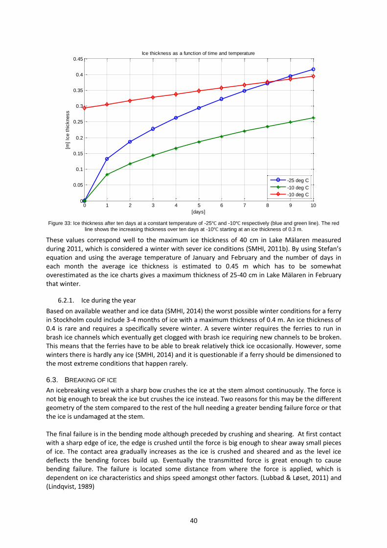
40
Figure 33: Ice thickness after ten days at a constant temperature of -25℃ and -10℃ respectively (blue and green line). The red
line shows the increasing thickness over ten days at -10℃ starting at an ice thickness of 0.3 m.
These values correspond well to the maximum ice thickness of 40 cm in Lake Mälaren measured during 2011, which is considered a winter with sever ice conditions (SMHI, 2011b). By using Stefan’s equation and using the average temperature of January and February and the number of days in each month the average ice thickness is estimated to 0.45 m which has to be somewhat overestimated as the ice charts gives a maximum thickness of 25-40 cm in Lake Mälaren in February that winter.
6.2.1. Ice during the year
Based on available weather and ice data (SMHI, 2014) the worst possible winter conditions for a ferry in Stockholm could include 3-4 months of ice with a maximum thickness of 0.4 m. An ice thickness of 0.4 is rare and requires a specifically severe winter. A severe winter requires the ferries to run in brash ice channels which eventually get clogged with brash ice requiring new channels to be broken. This means that the ferries have to be able to break relatively thick ice occasionally. However, some winters there is hardly any ice (SMHI, 2014) and it is questionable if a ferry should be dimensioned to the most extreme conditions that happen rarely.
6.3. BREAKING OF ICE
An icebreaking vessel with a sharp bow crushes the ice at the stem almost continuously. The force is not big enough to break the ice but crushes the ice instead. Two reasons for this may be the different geometry of the stem compared to the rest of the hull needing a greater bending failure force or that the ice is undamaged at the stem. The final failure is in the bending mode although preceded by crushing and shearing. At first contact with a sharp edge of ice, the edge is crushed until the force is big enough to shear away small pieces of ice. The contact area gradually increases as the ice is crushed and sheared and as the level ice deflects the bending forces build up. Eventually the transmitted force is great enough to cause bending failure. The failure is located some distance from where the force is applied, which is dependent on ice characteristics and ships speed amongst other factors. (Lubbad & Løset, 2011) and (Lindqvist, 1989)
0 1 2 3 4 5 6 7 8 9 100
0.05
0.1
0.15
0.2
0.25
0.3
0.35
0.4
0.45
[days]
[m]
Ice t
hic
kness
Ice thickness as a function of time and temperature
-25 deg C
-10 deg C
-10 deg C

41
The broken pieces (cusps or wedges) start rotating downwards as soon as they are formed. The cusps continue to rotate until they are parallel with the hull. During the rotation the newest cusps pushes previously formed pieces further aft along the hull. During the rotating process two important phenomena occurs.
1. Ventilation occurs when seawater is unable to immediately fill the gap between ice and hull.
The hydrodynamic forces acting on the broken ice (that interacts with the hull) is increased
and the global ship resistance increases accordingly.
2. The hull may experience significant impact forces when the upper surface of the broken ice
impacts the hull at the end of the rotation.
Figure 34: Left: the bow of KV Svalbard interacting with the ice. Right: KV Svalbard hits the edge of a large ice floe/level ice
sheet and the breaking process is being initiated. From (Lubbad & Løset, 2011)
Figure 35: Left: after the initial contact between hull and ice, the ice is broken by bending failure. Right: The resulted broken ice.
Note how the ice is broken by radial cracks and by bending failure. From: (Lubbad & Løset, 2011)
The last component of icebreaking resistance comes from submersion of the broken ice and the resistance between ice and hull. Underwater observations show that a ship running in level ice has most of the hull covered by ice.
6.4. ICE PROPERTIES
The ice has a number of mechanical properties that varies with the temperature, the volume of brine, growing process etc. (Timco & O’Brien, 1994). Ice properties are important factors affecting the hull-ice interaction and some of the most influential factors are described in this section.
6.4.1. Flexural strength
The research done about flexural strength of ice is mainly focused on sea ice as there are a number of vessels and other marine structures operating in sea ice conditions. However, in some models the
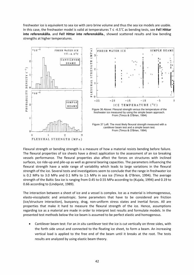
42
freshwater ice is equivalent to sea ice with zero brine volume and thus the sea ice models are usable. In this case, the freshwater model is valid at temperatures T ≤ -4.5˚C as bending tests, see Fel! Hittar inte referenskälla. and Fel! Hittar inte referenskälla., showed scattered results and low bending strengths at higher temperatures.
Figure 36 Above: Flexural strength versus the temperature of the
freshwater ice measured by using the simple beam approach. From (Timco & O’Brien, 1994)
Figure 37 Left: The most likely flexural strength measured with a
cantilever beam test and a simple beam test. From (Timco & O’Brien, 1994)
Flexural strength or bending strength is a measure of how a material resists bending before failure. The flexural properties of ice sheets have a direct application to the assessment of an ice breaking vessels performance. The flexural properties also affect the forces on structures with inclined surfaces, ice ride-up and pile-up as well as general bearing capacities. The parameters influencing the flexural strength have a wide range of variability which leads to large variations in the flexural strength of the ice. Several tests and investigations seem to conclude that the range in freshwater ice is 0.2 MPa to 3.0 MPa and 0.1 MPa to 1.5 MPa in sea ice (Timco & O’Brien, 1994). The average strength of the Baltic Sea ice is ranging from 0.45 to 0.55 MPa according to (Kujala, 1994) and 0.19 to 0.66 according to (Lindqvist, 1989). The interaction between a sheet of ice and a vessel is complex. Ice as a material is inhomogeneous, elasto-viscoplastic and anisotropic. Some parameters that have to be considered are friction (ice/structure interaction), buoyancy, drag, non-uniform stress states and inertial forces. All are properties that make it hard to measure the flexural strength of the ice. Hence, assumptions regarding ice as a material are made in order to interpret test results and formulate models. In the presented test methods below the ice beam is assumed to be perfect elastic and homogenous.
Cantilever beam test: For an in situ cantilever test the ice is cut vertically on three sides, with
the forth side uncut and connected to the floating ice sheet, to form a beam. An increasing
vertical load is applied to the free end of the beam until it breaks at the root. The tests
results are analyzed by using elastic beam theory.
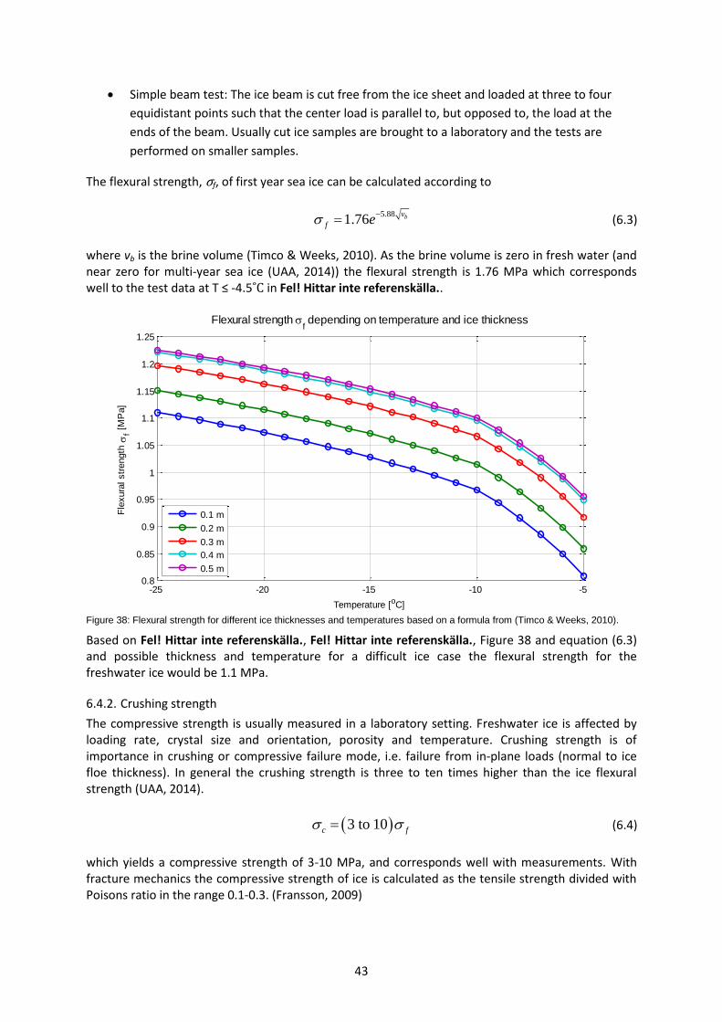
43
Simple beam test: The ice beam is cut free from the ice sheet and loaded at three to four
equidistant points such that the center load is parallel to, but opposed to, the load at the
ends of the beam. Usually cut ice samples are brought to a laboratory and the tests are
performed on smaller samples.
The flexural strength, σf, of first year sea ice can be calculated according to
5.88
1.76 bv
f e
(6.3)
where vb is the brine volume (Timco & Weeks, 2010). As the brine volume is zero in fresh water (and near zero for multi-year sea ice (UAA, 2014)) the flexural strength is 1.76 MPa which corresponds well to the test data at T ≤ -4.5˚C in Fel! Hittar inte referenskälla..
Figure 38: Flexural strength for different ice thicknesses and temperatures based on a formula from (Timco & Weeks, 2010).
Based on Fel! Hittar inte referenskälla., Fel! Hittar inte referenskälla., Figure 38 and equation (6.3) and possible thickness and temperature for a difficult ice case the flexural strength for the freshwater ice would be 1.1 MPa.
6.4.2. Crushing strength
The compressive strength is usually measured in a laboratory setting. Freshwater ice is affected by loading rate, crystal size and orientation, porosity and temperature. Crushing strength is of importance in crushing or compressive failure mode, i.e. failure from in-plane loads (normal to ice floe thickness). In general the crushing strength is three to ten times higher than the ice flexural strength (UAA, 2014).
3 to 10c f (6.4)
which yields a compressive strength of 3-10 MPa, and corresponds well with measurements. With fracture mechanics the compressive strength of ice is calculated as the tensile strength divided with Poisons ratio in the range 0.1-0.3. (Fransson, 2009)
-25 -20 -15 -10 -50.8
0.85
0.9
0.95
1
1.05
1.1
1.15
1.2
1.25
Flexural strength f depending on temperature and ice thickness
Temperature [oC]
Fle
xura
l str
ength
f [
MP
a]
0.1 m
0.2 m
0.3 m
0.4 m
0.5 m

44
6.4.3. Elastic modulus and Poisson’s ratio
Applying Hook’s Law on ice results in a tensile strength of 1 MPa and an elastic modulus of 5 to 9 GPa. Ice and many other brittle materials have a higher compressive strength than tensile strength. The elastic modulus of ice has been investigated in several experiments and in some cases it has been reported to be as high as 11.7 GPa at -10℃ (Petrovic, 2003). The Poisson’s ratio seems to be averaged around 0.3 in most tests. In the tests and simulations in this report the elastic modulus is set to 7 GPa and Poisson’s ratio is taken to be 0.3.

45
7. ICE BREAKING AND BRASH ICE RESISTANCES A vessels resistance when breaking ice is determined by the shape of the bow, the speed at which the vessel is breaking ice and ice characteristics. The brash ice resistance is also dependent on these factors. The resistance models gives an initial idea about the efficiency of the vessel operating in ice, but should be supplemented with model tests in an ice towing tank. The resistance models are used to design the bow section of the commuter vessel. The models estimates the ice resistance, however, the total resistance includes the open water resistance Row as well. The total resistance is calculated as
tot ow iR R R . (7.1)
The icebreaking models and brash ice resistance models have been verified against numerical simulations and measurement data from trials. The models give an average resistance and the result is quite consistent with the measurements differing by less than 10 % (Lubbad & Løset, 2011).
7.1. PARAMETERS IN CALCULATIONS
The models share a number of parameters, all parameters and in which model they are included are shown in Table 27. The resistance models have been made with merchant vessels and icebreakers in consideration. However, the Lindqvist (Lindqvist, 1989) resistance model has been tested for smaller vessels (length over all 15 m) and thus, it is used in this investigation. The other resistance model by Riska (Riska, Willhelmson, Englund, & Leiviskä, 1997) is tested and compared to Lindqvist’s model and the results are similar for larger and smaller vessels. The methods have been tested against measurement data collected for different vessels and yields similar result.
7.1.1. Angles in resistance calculations
The vessel’s parameters are defined as in Figure 39. The water plane entrance angle α at the waterline is taken as an average in the Lindqvist model, and can be taken as α at B/4. In Riska’s models for resistance the angle α is excluded as there are contradictory theories on its influence on the resistance. The flare angle ψ is calculated using the water entrance angle and the stem angle at B/4;
tan
arctansin
(7.2)
Figure 39: Definition of vessel’s parameters. From (FSICR, 2014)
ϕ

46
Table 25: Parameters and symbols used in the different resistance and load models.
Description Value Unit Symbol Lindqvist Icebreaking resistance
Riska Icebreaking resistance
Riska brash ice resistance
Beam 7.8 [m] B x x x
Length over all 26.8 [m] L x x x
Draught 1.5 [m] T x x x
Length of parallel mid body
4 [m] Lpar x x
Length of bow section 13 [m] Lbow x
Water plane area of bow section
[m2] AWF x
Ice thickness 0-0.5 [m] hi x x
Brash is thickness in the middle of the channel
0-1.5 [m] HM x
Gravity 9.81 [m/s2] g x x
Vessel’s speed 0-6 [m/s] V x x x
Water entrance angle 13-38 [°] α x x
Slope angle of brash ice
2.0 [°] γ x
Slope angle of side wall of brash ice
22.6 [°] δ x
Stem angle 15-35 ϕ x x x
Density of freshwater ice at -5℃
0.917 [t/m3] ρi x
Density of freshwater at 0℃
1 [t/m3] ρw x
Density difference between water and ice
0.083 [t/m3] ρ∆ x x
Flexural strength of ice
[MPa] σf x
Ice crushing strength [MPa] σc
Poisson’s ratio 0.3 [-] υ x
Elastic modulus 7 [GPa] E x
Friction between hull and ice
0.1 𝜇 x x
Empirical coefficient 0.8 𝜇B x
Empirical coefficient 0.68 Ko x
Empirical coefficient 6.5 Kp x
7.2. LINDQVIST ICEBREAKING RESISTANCE
The Lindqvist (Lindqvist, 1989) icebreaking resistance is commonly used for prediction of icebreaking resistance. Most information in this section is based on (Lindqvist, 1989) and (Martio, 2007). The ice resistance model is based on a number of factors such as the vessels geometry and speed, as well as ice properties and ice thickness.
The calculated loads in this model are the crushing force of the ice at the stem Rc, the breaking resistance Rb when breaking the ice cusps and a submersion resistance Rs that comes from the

47
friction caused by the broken ice being submersed and sliding along the hull under water. The model is based on the assumption that the deflection of the ice and the trim of the vessel can be ignored. The assumption can cause an underestimation of breaking resistance in very thick ice, in which the vessel trims considerably. But in the case of the smaller ferry operating in Stockholm the ice is thin enough for the assumption to be valid. An icebreaking vessel with a sharp bow crushes the ice at the stem almost continuously. The vertical force is not big enough to break the ice but the horizontal force crushes the ice instead. The average vertical force acting on the ice is
20.5v f iF h , (7.3)
Where hi is the ice thickness and σf is the ice flexural strength. By assuming that the friction force acts along the verticals the crushing resistance component RC is obtained as
costan
cos
cos1
sin
C vR F
, (7.4)
where μ is the friction between hull and ice, ϕ is the stem angle and ψ is the flare angle. The breaking resistance component describes the process of bending failure for the ice. The breaking resistance component is obtained as
2
27 tan cos 11
64 cos sin cos
12 1
if
w
hR B
E
g
B , (7.5)
where υ is Poissins coefficient and ρw is the water density and E Young’s modulus. The submersion resistance component caused by displacing the ice vertically and sliding it along the hull is expressed as
S w i totR g h B K , (7.6)
where ρi is the density of freshwater ice and g is the constant of gravity. The parameter K is calculated according to
2 2
1 10.7 cos cos
2 tan 4 tan sin tan
B T T BK T L T
B T
(7.7)
The total ice breaking resistance is expressed as
1.4 9.4
1 1i C B S
i
V VR R R R
g h g L
, (7.8)
The icebreaking resistance for different ice thicknesses and speeds are presented in Figure 40. It should be noted that icebreaking is usually done at low speeds as the resistance otherwise becomes
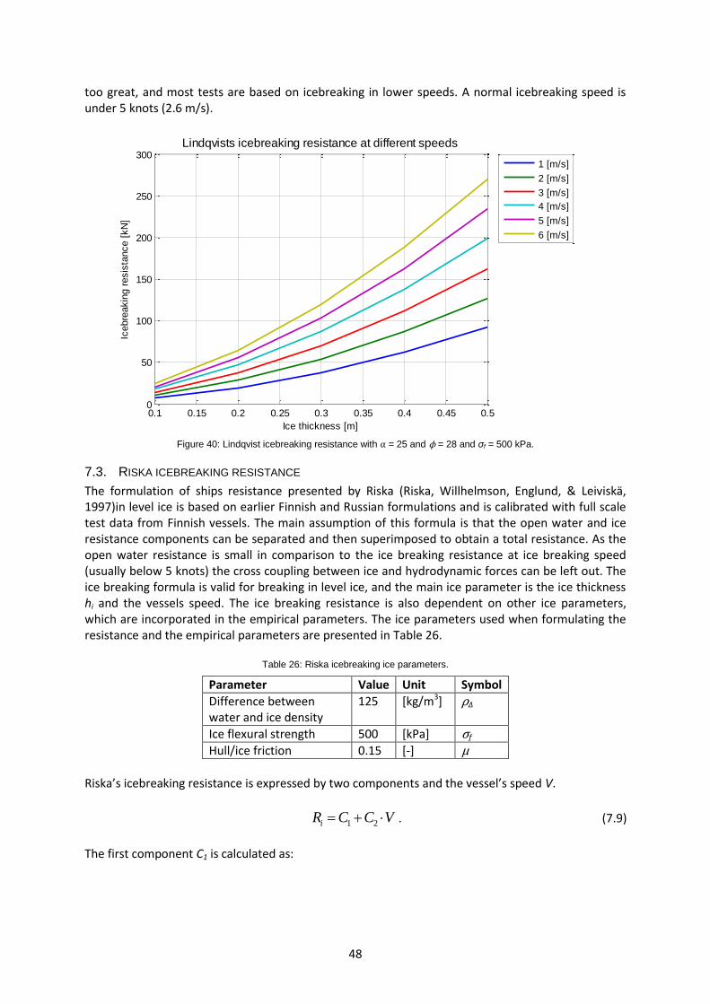
48
too great, and most tests are based on icebreaking in lower speeds. A normal icebreaking speed is under 5 knots (2.6 m/s).
Figure 40: Lindqvist icebreaking resistance with α = 25 and ϕ = 28 and σf = 500 kPa.
7.3. RISKA ICEBREAKING RESISTANCE
The formulation of ships resistance presented by Riska (Riska, Willhelmson, Englund, & Leiviskä, 1997)in level ice is based on earlier Finnish and Russian formulations and is calibrated with full scale test data from Finnish vessels. The main assumption of this formula is that the open water and ice resistance components can be separated and then superimposed to obtain a total resistance. As the open water resistance is small in comparison to the ice breaking resistance at ice breaking speed (usually below 5 knots) the cross coupling between ice and hydrodynamic forces can be left out. The ice breaking formula is valid for breaking in level ice, and the main ice parameter is the ice thickness hi and the vessels speed. The ice breaking resistance is also dependent on other ice parameters, which are incorporated in the empirical parameters. The ice parameters used when formulating the resistance and the empirical parameters are presented in Table 26.
Table 26: Riska icebreaking ice parameters.
Parameter Value Unit Symbol
Difference between water and ice density
125 [kg/m3] ρΔ
Ice flexural strength 500 [kPa] σf
Hull/ice friction 0.15 [-] μ Riska’s icebreaking resistance is expressed by two components and the vessel’s speed V.
1 2iR C C V . (7.9)
The first component C1 is calculated as:
0.1 0.15 0.2 0.25 0.3 0.35 0.4 0.45 0.50
50
100
150
200
250
300Lindqvists icebreaking resistance at different speeds
Ice thickness [m]
Icebre
akin
g r
esis
tance [
kN
]
1 [m/s]
2 [m/s]
3 [m/s]
4 [m/s]
5 [m/s]
6 [m/s]

49
2
1 1 2 4
11 0.0021
21
par i i bow iC f B L h f B h f B L hT
B
, (7.10)
where T is draught, B is the beam, Lpar is the parallel length of the mid body, Lbow is the length of the bow section, ϕ is the stem angle and the rest of the parameters are empirical coefficient presented in Table 27. The second component is
2
1.5
2 1 3 31 0.063 1 1.2i i i
T BC g h g B h g h
B L
.
(7.11)
Table 27: Empirical coefficients for Riska’s resistance.
Constant Value Unit
f1 0.23 [kN/m3]
f2 4.58 [kN/m3]
f3 1.47 [kN/m3]
f4 0.29 [kN/m3]
g1 18.9 [kN/(m/sm1.5)]
g2 0.67 [kN/(m/sm2)]
g3 1.55 [kN/(m/sm2.5)]
Figure 41: Icebreaking resistance with ϕ = 28°.
0.1 0.15 0.2 0.25 0.3 0.35 0.4 0.45 0.50
50
100
150
200
250
300Riska icebreaking resistance at different speeds
Ice thickness [m]
Icebre
akin
g r
esis
tance [
kN
]
1 [m/s]
2 [m/s]
3 [m/s]
4 [m/s]
5 [m/s]
6 [m/s]
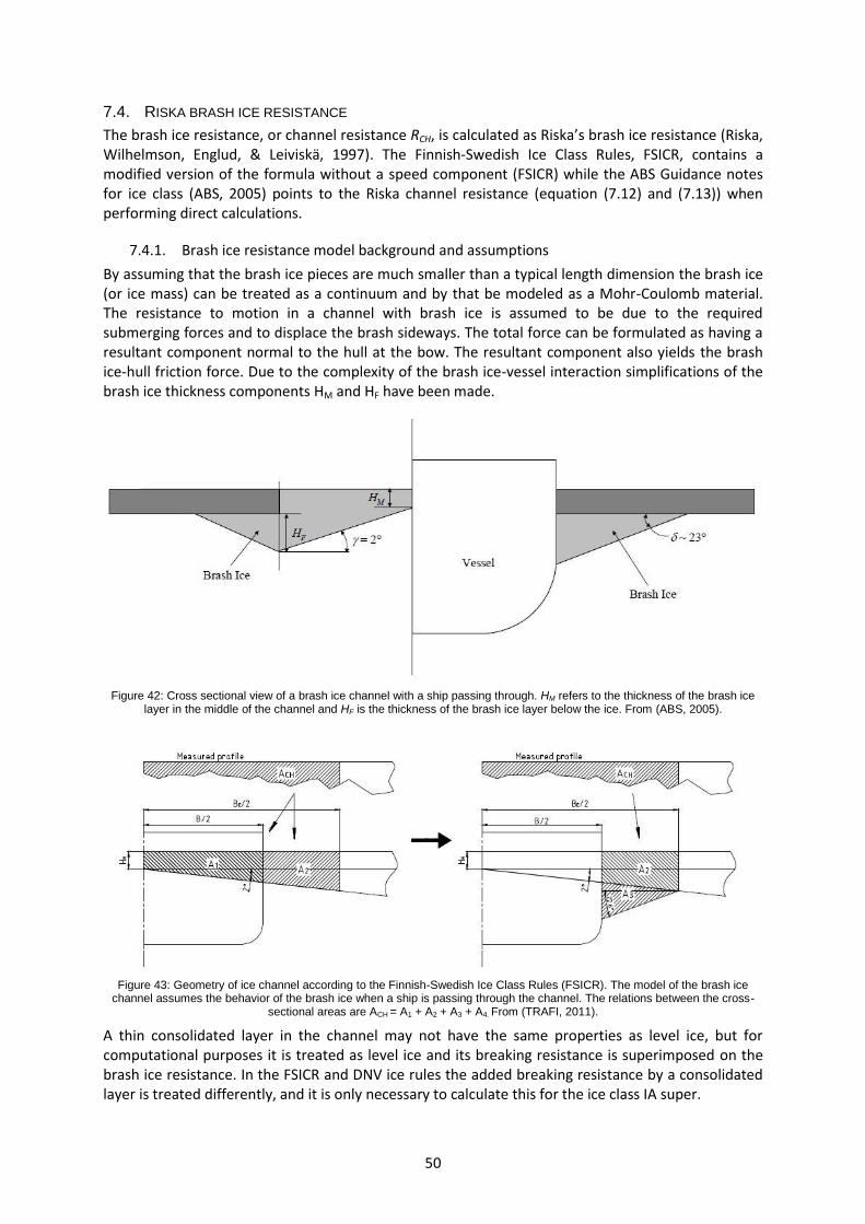
50
7.4. RISKA BRASH ICE RESISTANCE
The brash ice resistance, or channel resistance RCH, is calculated as Riska’s brash ice resistance (Riska, Wilhelmson, Englud, & Leiviskä, 1997). The Finnish-Swedish Ice Class Rules, FSICR, contains a modified version of the formula without a speed component (FSICR) while the ABS Guidance notes for ice class (ABS, 2005) points to the Riska channel resistance (equation (7.12) and (7.13)) when performing direct calculations.
7.4.1. Brash ice resistance model background and assumptions
By assuming that the brash ice pieces are much smaller than a typical length dimension the brash ice (or ice mass) can be treated as a continuum and by that be modeled as a Mohr-Coulomb material. The resistance to motion in a channel with brash ice is assumed to be due to the required submerging forces and to displace the brash sideways. The total force can be formulated as having a resultant component normal to the hull at the bow. The resultant component also yields the brash ice-hull friction force. Due to the complexity of the brash ice-vessel interaction simplifications of the brash ice thickness components HM and HF have been made.
Figure 42: Cross sectional view of a brash ice channel with a ship passing through. HM refers to the thickness of the brash ice
layer in the middle of the channel and HF is the thickness of the brash ice layer below the ice. From (ABS, 2005).
Figure 43: Geometry of ice channel according to the Finnish-Swedish Ice Class Rules (FSICR). The model of the brash ice
channel assumes the behavior of the brash ice when a ship is passing through the channel. The relations between the cross-sectional areas are ACH = A1 + A2 + A3 + A4. From (TRAFI, 2011).
A thin consolidated layer in the channel may not have the same properties as level ice, but for computational purposes it is treated as level ice and its breaking resistance is superimposed on the brash ice resistance. In the FSICR and DNV ice rules the added breaking resistance by a consolidated layer is treated differently, and it is only necessary to calculate this for the ice class IA super.

51
Opposed to level ice breaking where the largest forces are at the stem, the entire bow interacts in the brash ice resistance by displacing the ice. Thus, an average hull angle calculated over the length of the bow would be most suitable as the bow is approximated as a wedge with straight sides.
7.4.2. The model
The model can be evaluated for different brash ice thicknesses, bow angles and speeds as the Froude number Fn is a component containing the speed. The channel resistance, RCH is calculated as
2
2
3
2 2
0 2
10.5 0.5 2 cos cos sin sin
2 tan
MCH B F P F
F
B par F M WF
HR gH K B H
H
LTgK L H g H A Fn
B
(7.12)
where K0 and Kp are empirical parameters with a value of 0.68 and 6.5 respectively, μB is 0.8, AWF is the water plane area of the bow, HM is the brash ice thickness in the middle of the channel, δ and γ are slope angles of the brash ice and are 22.6° and 2° respectively. The parameter HF is calculated as
tan
4tan tan tan
2 tan tan
M
F M
BB HBH H
(7.13)
The brash ice resistance varies little with the speed as seen in Figure 44.
Figure 44: Brash ice resistance with α = 25° and ϕ = 28°.
7.5. PARAMETER STUDY
The ice resistance models investigated in this section are based on empirical measurements in sea ice. In Riska’s resistance model a flexural strength of 500 kPa is integrated in the formula and in Lindqvist it is an input parameter. In order to compare the methods the flexural strength is set to 500
0 0.5 1 1.50
10
20
30
40
50
60
70
80
90Riska channel resistance
Brash ice thickness in middle of channel [m]
Bra
sh ice r
esis
tance [
kN
]
0 [m/s]
1 [m/s]
2 [m/s]
3 [m/s]
4 [m/s]
5 [m/s]
6 [m/s]
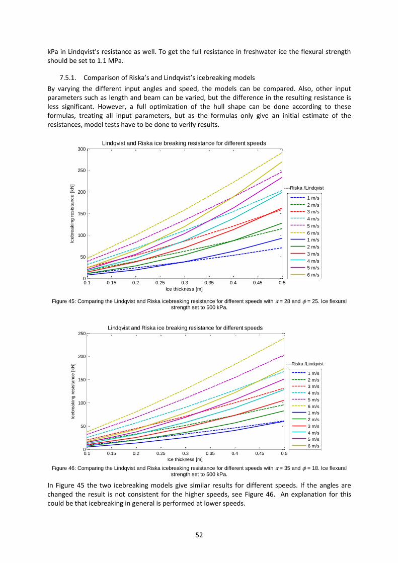
52
kPa in Lindqvist’s resistance as well. To get the full resistance in freshwater ice the flexural strength should be set to 1.1 MPa.
7.5.1. Comparison of Riska’s and Lindqvist’s icebreaking models
By varying the different input angles and speed, the models can be compared. Also, other input parameters such as length and beam can be varied, but the difference in the resulting resistance is less significant. However, a full optimization of the hull shape can be done according to these formulas, treating all input parameters, but as the formulas only give an initial estimate of the resistances, model tests have to be done to verify results.
Figure 45: Comparing the Lindqvist and Riska icebreaking resistance for different speeds with α = 28 and ϕ = 25. Ice flexural
strength set to 500 kPa.
Figure 46: Comparing the Lindqvist and Riska icebreaking resistance for different speeds with α = 35 and ϕ = 18. Ice flexural
strength set to 500 kPa.
In Figure 45 the two icebreaking models give similar results for different speeds. If the angles are changed the result is not consistent for the higher speeds, see Figure 46. An explanation for this could be that icebreaking in general is performed at lower speeds.
0.1 0.15 0.2 0.25 0.3 0.35 0.4 0.45 0.50
50
100
150
200
250
300
Ice thickness [m]
Icebre
akin
g r
esis
tance [
kN
]
Lindqvist and Riska ice breaking resistance for different speeds
1 m/s
2 m/s
3 m/s
4 m/s
5 m/s
6 m/s
1 m/s
2 m/s
3 m/s
4 m/s
5 m/s
6 m/s
----Riska /Lindqvist
0.1 0.15 0.2 0.25 0.3 0.35 0.4 0.45 0.50
50
100
150
200
250
Ice thickness [m]
Icebre
akin
g r
esis
tance [
kN
]
Lindqvist and Riska ice breaking resistance for different speeds
1 m/s
2 m/s
3 m/s
4 m/s
5 m/s
6 m/s
1 m/s
2 m/s
3 m/s
4 m/s
5 m/s
6 m/s
----Riska /Lindqvist

53
Figure 47: Comparing the Lindqvist and Riska icebreaking resistance for different speeds with α = 28 and ϕ = 25. Ice flexural
strength set to 1.1 MPa for fresh ice in Lindqvist’s formula and 500 kPa in Riska’s.
Figure 48: Comparing the Lindqvist and Riska icebreaking resistance for different speeds with α = 35 and ϕ = 18. Ice flexural
strength set to 1.1 MPa for freshwater ice in Lindqvist’s formula and 500 kPa in Riska’s.
If the Lindqvist resistance formula is adjusted with the values for freshwater ice the resistance increases. This is expected as the freshwater ice is stronger than sea ice. On the other hand, the formulae are not based on freshwater ice from the beginning which makes it difficult to know if the magnitude of the resistance increase is reasonable. In Figure 48 the resistances are lower than in in Figure 47 due to better water entrance angle and stem angle for icebreaking. The difference in resistance between the models increase when α > ϕ. The models gives fairly similar result for the opposite angle relationship. In Figure 49 and Figure 50 it is seen that the stem angle has a greater influence according to Lindqvist than for Riska. Also, the ice flexural strength seems to increase the influence of the stem angle on the resistance in Lindqvist’s model. For the smallest stem angle (ϕ = 15°) the result for both models is
0.1 0.15 0.2 0.25 0.3 0.35 0.4 0.45 0.50
100
200
300
400
500
600
Ice thickness [m]
Icebre
akin
g r
esis
tance [
kN
]Lindqvist and Riska ice breaking resistance for different speeds
1 m/s
2 m/s
3 m/s
4 m/s
5 m/s
6 m/s
1 m/s
2 m/s
3 m/s
4 m/s
5 m/s
6 m/s
----Riska /Lindqvist
0.1 0.15 0.2 0.25 0.3 0.35 0.4 0.45 0.50
50
100
150
200
250
300
350
Ice thickness [m]
Icebre
akin
g r
esis
tance [
kN
]
Lindqvist and Riska ice breaking resistance for different speeds
1 m/s
2 m/s
3 m/s
4 m/s
5 m/s
6 m/s
1 m/s
2 m/s
3 m/s
4 m/s
5 m/s
6 m/s
----Riska /Lindqvist

54
similar when breaking thicker ice, see Figure 51 and Figure 52. According to Riska’s model it is seen that low stem angles and low speed is the key to a low resistance when breaking ice, see Figure 53.
Figure 49: Comparison of Riska’s and Lindqvist’s icebreaking resistance with water entrance angle α = 35. Ice flexural strength
set to 500 kPa.
Figure 50: Comparison of Riska’s and Lindqvist’s icebreaking models with water entrance angle α = 35. Ice flexural strength set
to 1.1 MPa for freshwater ice in Lindqvist’s formula and 500 kPa in Riska’s.
0.1 0.15 0.2 0.25 0.3 0.35 0.4 0.45 0.50
20
40
60
80
100
120
140
160
180
200
Ice thickness [m]
Icebre
akin
g r
esis
tance [
kN
]
Lindqvist and Riska icebreaking resistance for different angles at 2 m/s
15 [deg]
25 [deg]
35 [deg]
15 [deg]
25 [deg]
35 [deg]
----Riska /Lindqvist
0.1 0.15 0.2 0.25 0.3 0.35 0.4 0.45 0.50
50
100
150
200
250
300
350
400
Ice thickness [m]
Icebre
akin
g r
esis
tance [
kN
]
Lindqvist and Riska icebreaking resistance for different angles at 2 m/s
15 [deg]
25 [deg]
35 [deg]
15 [deg]
25 [deg]
35 [deg]
----Riska /Lindqvist

55
Figure 51: Lindqvist’s icebreaking resistance with water entrance angle fixed at α = 28 and ice flexural strength set to 500 kPa.
Figure 52: Riska’s icebreaking resistance with fixed ice flexural strength (500 kPa).
0.1 0.15 0.2 0.25 0.3 0.35 0.4 0.45 0.50
20
40
60
80
100
120
140
160
180
200
Lindqvists model varying at 2 m/s
Ice thickness [m]
Ice b
reakin
g r
esis
tance [
kN
]
15 [deg]
20 [deg]
25 [deg]
30 [deg]
35 [deg]
0.1 0.15 0.2 0.25 0.3 0.35 0.4 0.45 0.50
20
40
60
80
100
120
140
Riska icebreaking resistance varying at 2 m/s
Ice thickness [m]
Icebre
akin
g r
esis
tance [
kN
]
15 [deg]
20 [deg]
25 [deg]
30 [deg]
35 [deg]

56
Figure 53: Riska’s icebreaking resistance. Ice flexural strength set to 500 kPa.
Figure 54: Lindqvist’s icebreaking resistance with stem angle fixed at ϕ = 25.
The water entrance angle has less influence than the stem angle according to Lindqvist’s model. This result corresponds to the Riska ice breaking model where the water entrance angle is excluded as its influence is not certain. A small stem angle seems to give the least resistance according to the Lindqvist resistance model, see Figure 55 and Figure 56. It is also seen that the difference in ice flexural strength significantly increases the resistance. At this speed and ice thickness it appears the resistance increases linearly with the flexural strength.
10 20 30 40 50 60 70 80 90
0
2
4
6
0
100
200
300
400
[o]
Riska icebreaking resistance in 0.35 m level ice
V [m/s]
Resis
tance [
kN
]
50
100
150
200
250
300
350
0.1 0.15 0.2 0.25 0.3 0.35 0.4 0.45 0.50
20
40
60
80
100
120
140
160
180
Lindqvists model varying at 2 m/s
Ice thickness [m]
Ice b
reakin
g r
esis
tance [
kN
]
18 [deg]
23 [deg]
28 [deg]
33 [deg]
38 [deg]

57
Figure 55: Lindqvist’s icebreaking resistance with ice flexural strength is set to 500 kPa.
Figure 56: Lindqvist’s icebreaking resistance with ice flexural strength set to 1.1 MPa for freshwater.
1020
3040
5060
10
20
30
40
50
0
200
400
600
800
Lindqvist icebreaking resistance in 0.35 m level ice at 2 m/s
Resis
tance [
kN
]
100
200
300
400
500
600
700
1020
3040
5060
10
20
30
40
500
500
1000
1500
2000
Lindqvist icebreaking resistance in 0.35 m level ice at 2 m/s
Resis
tance [
kN
]
200
400
600
800
1000
1200
1400
1600

58
7.5.2. Brash ice resistance
The brash ice resistance is dependent on the bow angles. The stem angle has a greater effect on the result than the water entrance angle. It seems like the speed magnifies the effect of the water entrance angle α when comparing Figure 57 to Figure 58.
Figure 57: Brash ice resistance with the stem angle fixed at ϕ = 28. Note the small difference in resistance for when varying
angle α.
Figure 58: Brash ice resistance with the stem angle fixed at ϕ = 25. Note that the variation in resistance due to the change of
angle α is small and only noticeable at a thicker layer of brash.
The stem angles influence on the resistance is quite significant as seen in Figure 59 and Figure 60. For a stem angle of 13° it is seen that the brash ice resistance first increase until the brash ice thickness is 1 m before the resistance decrease for brash ice thicknesses greater than 1 m. This suggests the model is not valid at angles as low as 13°.
0 0.5 1 1.50
10
20
30
40
50
60
70
80
90
Riska brash ice resistance as a function of at 2 m/s
Brash ice thickness in middle of channel [m]
Bra
sh ice r
esis
tance [
kN
]
15 [deg]
20 [deg]
25 [deg]
30 [deg]
35 [deg]
0 0.5 1 1.50
10
20
30
40
50
60
70
80
90
Riska brash ice resistance as a function of at 5 m/s
Brash ice thickness in middle of channel [m]
Bra
sh ice r
esis
tance [
kN
]
18 [deg]
23 [deg]
28 [deg]
33 [deg]
38 [deg]

59
Figure 59: Brash ice resistance with fixed water entrance angle α = 25°.
Figure 60: Brash ice resistance with fixed water entrance angle α = 25°.
The results in Figure 61 shows that the brash ice resistance is not so depending on speed for the angles α = 28° and ϕ = 25°. The result is not expected and trials should be done to verify the results,
0 0.5 1 1.50
20
40
60
80
100
120
Riska brash ice resistance as a function of at 2 m/s
Brash ice thickness in middle of channel [m]
Bra
sh ice r
esis
tance [
kN
]
13 [deg]
18 [deg]
23 [deg]
28 [deg]
33 [deg]
38 [deg]
0 0.5 1 1.50
20
40
60
80
100
120
140
Riska brash ice resistance as a function of at 5 m/s
Brash ice thickness in middle of channel [m]
Bra
sh ice r
esis
tance [
kN
]
13 [deg]
18 [deg]
23 [deg]
28 [deg]
33 [deg]
38 [deg]

60
Figure 61: Riska brash ice/channel resistance.
To further investigate the brash ice resistance the resistance is plotted for a fixed speed and brash ice thickness but varied bow angles, see Figure 62. For low ϕ and high α the resistance is negative which suggests these combination of angles are outside the valid interval for the model.
Figure 62: Riska’s brash ice resistance.
0 0.5 1 1.50
10
20
30
40
50
60
70
80
90Riska channel resistance
Brash ice thickness in middle of channel [m]
Bra
sh ice r
esis
tance [
kN
]
0 [m/s]
1 [m/s]
2 [m/s]
3 [m/s]
4 [m/s]
5 [m/s]
6 [m/s]
15 20 25 30 35 40 45 50 55
0
50
100
-200
0
200
400
600
Resistance in 2 m brash at 6 m/s
Bra
sh ice r
esis
tance [
kN
]
-100
0
100
200
300
400
500

61
7.6 DISCUSSION ON RESISTANCE MODELS
The largest difficulty in judging the reliability of the results is that almost no research or tests on icebreaking and ice going vessels in freshwater has been done. On the other hand, multi-year sea ice can have a low brine volume due to brine drainage and therefore be almost as tough as freshwater ice. Ice properties are difficult to define and research within this area is also focused on sea ice. However, the chosen ice properties are within reasonable limits according to formulas and measurements. The properties are chosen to represent a level ice sheet with ice of high flexural and crushing strength as this kind of ice is the “worst case” that could be encountered. To make sure that the correct properties of the ice are chosen tests on ice from Lake Mälaren should be carried out. Also the flexural strength is taken as a worst case scenario and could be somewhat over estimated. The Lindqvist’s formula is regarded as a first calculation of ships icebreaking resistance. The formula is commonly used as a first assumption and further investigations have to be made in order to verify the results. However, the formula has been used in scientific studies since it was first presented in the late 80’s which indicates its predictions are fairly reliable. The Lindqvist formula has been used in a number of studies where the input data is presented along with the results. The data provided has enabled the model used in the resistance investigations to be tuned in to give the correct values. As the ice flexural strength can be varied in the Lindqvist formula it was set to 500 kPa when Riska’s icebreaking resistance formula was tuned to fit the Lindqvist formula. The main drawback of using these formulae is that they are intended for vessels significantly larger than the commuter ferry and have not been thoroughly evaluated for smaller vessels. The models are also made for vessels with conventional merchant vessel hulls or icebreaker hulls. This makes the models less reliable for smaller vessels. However, the Lindqvist formula has been used to estimate the resistance for vessels as small as 15 m and also for icebreaking ferries with an estimated resistance close to the measured. The reason the resistance models are used although they are not specifically designed for the commuter ferry is that there are no other methods for estimating resistances for small vessels other than testing. With the Riska icebreaking formula having some pre-determined values such as the ice flexural strength set, it makes this formula less adaptable to other ice conditions than sea water ice. It is clear that the increased flexural strength in freshwater ice increases icebreaking resistance in the Lindqvist formula. The increased flexural strength that is found both in old or multi-year sea ice and freshwater ice is scientifically proved which leads to the conclusion that Lindqvist’s formula is more appropriate to use in the case of the ice going commuter vessel. Another concern of the ice breaking resistance formulae is the dependence on the angles of the bow. It is clear that some combinations of ϕ and 𝛼 give a result that is not reliable as the Lindqvist formula spikes at high ϕ and does not increase linearly with increasing stem angle. The same goes for the Riska brash ice resistance where low water entrance angle (α = 13°) yields a negative resistance when the brash layer is thick enough. It is noticeable that the bow angles have some impact on the resistance, both in ice breaking and running in brash ice, but how much impact changes for the different formula. For α = 25° and ϕ = 28° both icebreaking formulae yields similar results, but for other angle combinations the result varies. Riska’s formula does not include the water entrance angle; the theory behind this is that is not significant for the result. In Lindqvist’s formula the different angle combinations are possible as the principle is that the geometry of the entire bow is affecting the resistances. With regards to how the bow of icebreakers is designed it is quite clear that the entire bow is designed to minimize icebreaking resistance and therefore the water entrance angle could have some influence in the resistance. How much is not clear, but the design formulae should be used for an initial design and further tests and trails should be done to verify the design. It is not clear why the difference in

62
resistance for the two icebreaking models increase when α > ϕ and further investigations to find the reason for this has to be performed. It is also seen that the Lindqvist formula is more dependent on the angles and the results vary more than for Riska’s icebreaking resistance, see Figure 49 and Figure 50. The variation of the angles influence on the formulae makes it difficult to know which method to use to determine the appropriate angles of the bow. In general both methods point towards that a low stem angle reduces resistance, which is in line with the ice having a lower flexural strength than crushing strength. Thus, bending failure comes before crushing failure and by designing the bow to “slide” on top of the ice and transfer force downwards instead of crushing the ice head on yields less resistance. A bow optimized for icebreaking might increase the open water and channel resistance. Therefore it is important to calculate the vessels properties in other conditions than icebreaking, especially for a commuter vessel in Stockholm that runs in open water for a minimum of 8 months of the year, before deciding on a bow shape for the vessel. The icebreaking resistance’ speed dependence seems to vary by the same magnitude for both formulae when Lindqvist’s formula had the properties for freshwater ice, see Figure 47 and Figure 48. When both formulae had the ice flexural strength set to 500 kPa the Riska formula was more influenced by the speed, see Figure 45 and Figure 46. As the resistance increases quite dramatically at higher speeds for the same ice thickness it is not advisable to break ice at high speeds. Also, there are less data on icebreaking at higher speeds which could make the formulae less correct. Icebreaking also requires stronger machinery than running in channels and open water and one way of not having a fleet of commuter vessels with icebreaking capacities running with oversized engines for open water is to limit the icebreaking capacities to a few vessels and use them as icebreakers. The brash ice resistance is interesting as it contains a speed parameter which enables the resistance to be evaluated for higher speeds. Surprisingly the speed of the vessels does not have a significant effect on the resistance; it is the bow angles who contribute to the resistance. Of the three resistance models, the brash ice resistance is the most sensitive to the design of the bow. For a channel with a 1.5 m thick brash ice layer the resistance is between 45 and 125 kN depending on the stem angle ϕ (18° to 38°). The water entrance angle has less influence on the resistance. Depending on the operational profile the vessel should be investigated for brash ice resistance more fully. It is worth comparing breaking new channels often or keep on running in channels until they are filled with more brash ice, requiring a larger propulsion machinery for the vessels that only run in channels and not break ice. The main conclusion is that the ice breaking and brash ice resistance models can serve as a tool at the first design stage evaluating the resistance that the vessel could encounter. The models are not fully tested for small vessels and the Riska ice breaking formula does not take the increased flexural strength for freshwater ice into account. The design of the bow has impact on the total resistance of the vessel. Further tests have to be done to verify that the Lindqvist resistance formula is better suited for evaluating small vessels.

63
8. ICE LOADS AND LOAD AREA DEFINITION Any structure interacting with sea or lake ice is subjected to loads on the structure. Either the structure is fixed and the loads are caused by the movements of the ice or the structure moves through the ice. In either case the loads on the structure are ruled by the same principles. The ice loads are dimensioning for the structure. Ice loads have been measured with strain gauges, pressure sensors and more and the result is clear that the ice loads vary randomly. It has even been suggested that some parameters that rule the ice loads could be varied randomly and simulate the loads with a Monte Carlo method (Palmer, Dempsey & Masterson, 2009), (Kujala, 1994).
8.1. DEFINITION OF LOAD AREA
There are several definitions of load area used to describe ice pressure and area in use in the research on ice loads. The global pressure is related to the global (or nominal) area. The global area is defined as the area that develops during the hull-ice interaction. Simply put is it the area of the structure projected onto the dimensions of the ice feature at the appropriate amount of ice penetration (Timco & Sudom, 2013). According to (Masterson & Frederking, 1992) the global load is identical to the local when contact occurs over the full thickness of the ice. A local pressure occurs over defined smaller portion of a larger global area. Generally the pressure is calculated using the maximum ice load on the corresponding assumed local contact area. Due to the ice inhomogeneous mechanical properties the actual loaded area is quite hard to measure and define (Timco & Sudom, 2013) and (Fransson, 2009). The larger local pressure area has a proposed aspect ratio of 8:1 (width of loaded area/height of loaded area) (Masterson & Frederking, 1992) when designing ships for Arctic conditions. The local loaded area is inside a larger global area of possible ice contact and its confinement conditions can be quite different than that for global pressure. The local loads are applied over an area which is usually far from a free edge of the ice sheet. A size or scale effect phenomenon has been found, which means the local pressure increases with decreased loaded area (Masterson & Frederking, 1992), (Masterson, Frederking, Wright, Kärnä & Maddock, 2007). As the loaded area increase it becomes difficult to distinguish a local load from a global load and two load cases could easily get mixed. However, as the scale effect phenomena indicate it has important implications for the design of hull structures since only smaller areas has to withstand the higher pressures (Jordaan, 2001). This yields that the structural design can be designed to withstand significantly lower pressures (Palmer, Dempsey & Masterson, 2009). During hull-ice interaction a force over a smaller (local) area M is measured, see Figure 63. However, M might not be determined by M alone but depend on a larger area D, or indeed an even larger area S (Palmer, Dempsey & Masterson, 2009).
Figure 63: Schematic illustration of the pressure area definition.

64
The pressure-area relationship assumes that M and S are coterminous, which is an idealization of the definition of the load area (Timco & Sudom, 2013). The pressure-area relationship is governed by the mechanical properties of ice rather than the mechanics of the structure in contact with the ice. In order for this statement to be true it is assumed that the structure is neither weak nor flexible (Palmer, Dempsey & Masterson, 2009). It is important to realize that the definition of load area does not fully describe the interaction process between ice and hull (Timco & Sudom, 2013); the schematic model in Figure 63 are according to some researchers over idealized (Palmer, Dempsey & Masterson, 2009). Despite this, the pressure-area approach gives useful information on the local pressures, and will be used to investigate and determine local pressures on the ferry hull. Full scale measurements of both local and global loads show great randomness in the sense that there is uncertainty associated with the process or value under consideration. By taking randomness in the ice response into account the simulation of loads becomes more accurate (Jordaan, 2001). Data from various types of structure-ice interaction indicates an average value of 7 MPa in small areas (0.045 m2) and an average pressure of 0.5-1.5 MPa in areas of 1-162 m2 (Johnston, Croasdle, & Jordaan, 1998). This means that high pressure zones offer a partial explanation for the trend of decreasing pressure with increasing area.
8.1.1. High pressure zones
The force between ice and structure is far from uniformly distributed and at any given time there is actually a number of high pressure zones (HPZs) at which most of the force is concentrated (Dempsey, Palmer, & Sodhi, 2001). The HPZs only occupy a small fraction of the nominal contact area. The HPZs form and disappear rapidly as well as jump around. These properties make HPZs complicated to predict and use in load area models. Some of the phenomena behind HPZs are different kinds of fracture, elastic and plastic deformation, recrystallization, pressure-melting and creep that happen simultaneously (Palmer, Dempsey & Masterson, 2009), (Jordaan, 2001). The simpler models describing HPZs are based on the assumption that only one HPZ is present within the area M over which the total force is measured. According to some tests (Jordaan, 2001) the zone in which the HZP are concentered in is around 0.1 m2, although sometimes smaller or larger.
Figure 64: High pressure zones. From (Jordaan, 2001)

65
Figure 65: High pressure zones. From (Jordaan, 2001)
The HPZ model disregard the assumption that the pressure-area relationship is based on, the assumption that the overall load area which the pressure is measured in is the same as the area that determines the pressure (Palmer, Dempsey & Masterson, 2009). As HPZs more accurately describe the real behavior of ice-structure interaction it would be suitable to use this model for determining extreme loads. However the HPZ models are also based on assumptions as the ice-structure interaction is ruled by an extensive amount of parameters that in some cases are interdependent.
8.1.2. High pressure zone load model
A model for describing the HPZ has been developed by (Palmer, Dempsey & Masterson, 2009) which handles one HPZ in a square area. The model assumes that the maximum force F that can be applied is limited by edge spalling. In Figure 66 the square face represent the loaded area S, and the dotted square is the loaded area M in Figure 63.
Figure 66: Left: square of elastic/brittle material and one high HPZ. Right: Logarithmic plot of the force factor against the area
factor. From (Palmer, Dempsey, & Masterson, A revised ice pressure-area curve and a fracture mechanics explanation, 2009).

66
The location of the HPZ is randomized as well as the area A and location of the square M. The largest forces per unit area occur when the HPZ is located at the middle of the side of the square S and the measurement area is small. By comparing the result in Figure 66 with the empirical data in Figure 67, it is clear that the simulation model of the pressures corresponds fairly well with the measurement data. Note that the design pressure curve (black dotted line) is the average pressure plus three standard deviations, which make the design-curve the highest possible pressure.
Figure 67: Local pressure area relationship for fixed structures. From (Timco & Sudom, 2013)
8.2. PRESSURE-AREA CURVE
By compiling experimental data on pressures and local load areas up to 7 m2 from field trials, laboratory experiments and ship trials, a pressure-area relationship was determined (Masterson & Frederking, 1992). Based on this, design curves for local design pressure can be obtained by using
0.5728.1 cp A , (8.1)
0.77.4 cp A , (8.2)
where p is the pressure and Ac is the loaded area. The second pressure equation (8.2) is based on (Masterson D. , Frederking, Wright, Kärnä, & Maddock, 2007) and takes the ISO 19906 Arctic Structure Standard into account. Both equations are based on large number of field research experiments and are assembled from the test data. The formulae are based on a regression line fitted to the average plus three standard deviations (Palmer, Dempsey & Masterson, 2009). However, equation (8.2) is not for vessels but for fixed structures. As seen in Figure 68 there is a difference in pressure for the two methods as the area decreases. The methods have not been validated below 0.1 m2 although the curve seems to follow measurement data to fairly well, see Figure 68.

67
Figure 68: Pressure-area curve.
For example, in ABS guidelines for icebreaking vessels (ABS, 2005) the maximum design pressure for line loads is 1.4819 MPa which yields a corresponding line load of 370.5 MN/mm. This pressure-area approach corresponds well with measurement data that the minimum average pressure is about 1.5 MPa for large contact areas. The pressure area curves give an average pressure for the load area although the pressure varies almost randomly and the peak pressure could be considerably higher.
8.2.1. Peak load distribution
During the hull-ice contact a crushing force takes place first and consequently the load-spike (peak load) is getting higher and higher. When the accumulated force is high enough to cause bending failure a sudden drop in load is observed (Suyuthi, Leira, & Riska, 2012). As seen in Figure 69 the high load-spikes are quite few compared to the total number of spikes. The line load in the figures is defined as the total load between two consecutive frames divided by the distance of the frames. An example of the load-spike distribution and at what value they peak at is seen in Figure 70. The figure is plotted as a logarithmic histogram (Biao, Riska, & Moan, 2011). Based on Figure 70 and Figure 69 as well as other experiments it is seen that the higher peak-loads are few in comparison to the lower peak-loads.
10-1
100
101
101
102
Pressure-area curve
[m2]
[MP
a]
Masterson 1992
Masterson 2007 (ISO 19906 Arctic Structures Standard)
0 1 2 3 4 5 6 7 8 9 100
20
40
60
80
[m2]
[MP
a]
Pressure-area curve
Masterson 1992
Masterson 2007 (ISO 19906 Arctic Structures Standard)
0 0.1 0.2 0.3 0.4 0.5 0.6 0.7 0.8 0.9 10
20
40
60
[m2]
[MP
a]
Pressure-area curve
Masterson 1992
Masterson 2007 (ISO 19906 Arctic Structures Standard)

68
Figure 69: typical time history of ice induced load on a vessel’s hull. From (Suyuthi, Leira, & Riska, 2012)
Figure 70: Distribution of peak loads on a frame on the bow of MT Uikku in an average ice thickness of 0.125 m, average ship
speed of 5.55 m/s, measured during a 10 min full scale trial during the winter 2003. From (Biao, Riska, & Moan, 2011)
8.3. LOAD CASE
The load cases are chosen to represent the ice loads encountered by the commuter vessel.
8.3.1. DNV load case
The first load case is the DNV design pressure used in the rules (DNV, 2012) to calculate the scantlings for the vessel. This pressure simulates the ice loads as a line load with a height of 22 cm along the entire waterline of the vessel. The DNV design pressure is 1 MPa for the specific area under investigation (5.4).
8.3.2. Load case 1, 2 and 3
The height of the loaded areas is assumed to be 15 cm as the spalling and breaking of edges of the ice prevents the loaded area height to become greater. The height corresponds well to the DNV ice rules where a line load in the ice belt is 20 cm high for ice class 1C (which is constructed for an ice thickness of 0.4 m). The vertical location of the ice belt varies with cargo load of the ferry. However, it is not considered in this analysis. The width of the loaded area varies; generally the pressure-area relationship yields the larger the area the lower the pressure with a minimum of 1.5 MPa. A distributed load of 1.5 MPa with a height of 15 cm along the length of the ice belt represents a background pressure. In order to simulate the actual load of the ice, HPZ’s are modeled as oval spots within the background pressure area. As the pressure of the HPZ seems to vary quite randomly, but the higher loads are quite rare, a pressure of
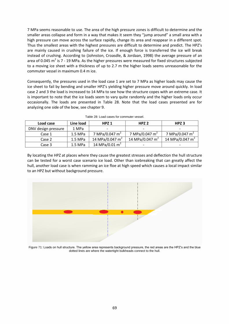
69
7 MPa seems reasonable to use. The area of the high pressure zones is difficult to determine and the smaller areas collapse and form in a way that makes it seem they “jump around” a small area with a high pressure can move across the surface rapidly, change its area and reappear in a different spot. Thus the smallest areas with the highest pressures are difficult to determine and predict. The HPZ’s are mainly caused in crushing failure of the ice. If enough force is transferred the ice will break instead of crushing. According to (Johnston, Croasdle, & Jordaan, 1998) the average pressure of an area of 0.045 m2 is 7 - 19 MPa. As the higher pressures were measured for fixed structures subjected to a moving ice sheet with a thickness of up to 2.7 m the higher loads seems unreasonable for the commuter vessel in maximum 0.4 m ice. Consequently, the pressures used in the load case 1 are set to 7 MPa as higher loads may cause the ice sheet to fail by bending and smaller HPZ’s yielding higher pressure move around quickly. In load case 2 and 3 the load is increased to 14 MPa to see how the structure copes with an extreme case. It is important to note that the ice loads seem to vary quite randomly and the higher loads only occur occasionally. The loads are presented in Table 28. Note that the load cases presented are for analyzing one side of the bow, see chapter 9.
Table 28: Load cases for commuter vessel.
Load case Line load HPZ 1 HPZ 2 HPZ 3
DNV design pressure 1 MPa - - -
Case 1 1.5 MPa 7 MPa/0.047 m2 7 MPa/0.047 m2 7 MPa/0.047 m2
Case 2 1.5 MPa 14 MPa/0.047 m2 14 MPa/0.047 m2 14 MPa/0.047 m2
Case 3 1.5 MPa 14 MPa/0.01 m2 - -
By locating the HPZ at places where they cause the greatest stresses and deflection the hull structure can be tested for a worst case scenario ice load. Other than icebreaking that can greatly affect the hull, another load case is when ramming an ice floe at high speed which causes a local impact similar to an HPZ but without background pressure.
Figure 71: Loads on hull structure. The yellow area represents background pressure, the red areas are the HPZ’s and the blue
dotted lines are where the watertight bulkheads connect to the hull.

70
8.4. DISCUSSION ON LOADS
The load models are mainly for larger vessels and another way of predicting local forces and the force impact area. The pressure-area approach is disregarding the geometry of the object but takes ice properties into account instead. The method is based on numerous tests performed on fixed structures, vessels and on test-panels being pushed into the ice. The collected data shows that the size of the loaded area and the magnitude of the load vary almost randomly and the pressure area curve only shows a mean value. The most problematic part of this data is that it is collected from tests where the ice thickness has been thicker than the worst possible ice thickness in Stockholm and therefore a thinner ice sheet might not cause loads as high as measured in the tests. Hence no extreme loads are chosen. High pressure zones describe how the ice behaves in a crushing/impact situation and would be the most realistic way of simulating an ice load as the HPZ’s takes into consideration the different possible failure modes of the ice. However, as they change in magnitude, size and location it is difficult to decide on appropriate load cases and an analysis should be made for a dynamic load case to fully understand how the loads influence the structure. A dynamic load could have a smaller effect on the structure and thus a static load case could overestimate the actual impact of an HPZ. A dynamic load case was not presented as a possible load case as the scope of this project does not contain a dynamic load analysis. The randomness of the measurement data from ice loads combined with the theory of HPZ’s led to the load cases presented in 8.3. The loads presented are possible, but how often they occur is not investigated. As seen in Figure 69 and Figure 70 the highest loads appear seldom, but a passenger vessel has to be able to cope with these high loads due to safety reasons. A step in further evaluation is to investigate how many of these extreme load cases the structure can cope with and dimension the structure to bear the loads during its lifetime. A severe load case is when the vessel is ramming a floe at full cruising speed (12 knots in this case). Load case 1-3 could also represent an impact load as there are local high loads. Impact loads mainly happens late on in the winter season when ice is breaking up due to weather changes causing thick floes to float around. The load cases are representative for a worst case load scenario but a dynamic analysis is advisable. Overall the information on ice loads and resistances, ice properties etc. has to be verified by tests in freshwater ice before they can be seen as reliable. The models are at the moment to be regarded as a first design guide before tests are carried out. (Timco & O'Brien, Flexural strength equation for sea ice, 1994) (Timco & Sudom, Revisiting the Sanderson pressure-area curve: Defining parameters that influence ice pressure, 2013) (Timco & Weeks, A review of the engineering properties of sea ice, 2010)

71
9. LOAD ANALYSIS WÅAB (Waxholmsbolaget) is aiming to build new vessels according to DNV ice class 1C, but the new commuter vessels fall outside the validity range of the rules. The aim is to test the vessel built according to DNV rules with the DNV design load and the analytic loads and compare the result.
9.1. MODEL
The starboard side of the bow section is modeled as a shell model in Creo Parametric 2.0. In a few locations extra stiffening structure is added to investigate how it can improve the structure under load. The load analysis is performed in Creo Simulate Academic Edition. Material selection, shell thicknesses, constraints and loads are applied in the simulation tool.
Figure 72: Thicknesses of hull structural members. The thickness of the red members are 8 mm, the blue and green members
are 15 mm and the yellow plates are 8 mm thick.
9.1.1. Assumptions and simplifications
The shell model is based on DNV design criteria. The hull and scantlings of the longitudinal and transversal girders and stiffeners are all according to the rules. However, the model is a conservative and comparatively simple structure with some simplifications.
No web frames
Thickness for water tight bulkheads not calculated
Hull structure not dimensioned for global loads
Few extra stiffening parts added, only added in regions close to high pressure zones
Manufacturing has not been taken into account
It is assumed that the simplifications made are not affecting the result of the loads notably.
9.1.2. Material
The structure is designed according to DNV design rules for steel NV-NS 235. The steel type has a failure stress limit of 235 MPa and an allowable stress (σa) limit of 156 MPa, which corresponds to a
Thickness:
8 mm 15 mm 15 mm 13 mm

72
safety factor of 1.5. The shell model can be analyzed with regard to membrane stresses and a combination of membrane and bending stresses giving the allowable stresses according to:
membrane stresses < σa
primary membrane + bending stresses < 1.5 σa
9.1.3. Boundary conditions
It is assumed that the keel adds stiffness to the structure and prevents the stiffeners, girders and bulkheads to rotate in any direction at the connecting point. Furthermore the keel is assumed to be stiffness enough to prevent it from displacing (or displacing only a negligible amount) when subjected to loads all in order to sustain the shape of the hull.
Figure 73: Boundary conditions.
9.2. LOAD CASE
The load cases to be run are based on ice loads purely. The sea pressure is around 40 kPa, which is negligible in comparison to the ice loads which are over 1 MPa. The first load case is the DNV design pressure which is a distributed load along the length of the investigated part of the ice belt with a width of 0.2 m. Load case 1 and 2 are based on semi-empirical load formulae and tests. The minimum distributed load is 1.5 MPa and local high pressure zones (HPZ) with areas from 0.01 m2 to 0.047 m2 and a pressure of 7 MPa each. The locations of the HPZ’s are chosen to represent the worst possible load cases. The load cases are described in full in 8.3.
Table 29: Load cases in FEA analysis.
Load case Line load HPZ 1 HPZ 2 HPZ 3
DNV design pressure 1 MPa - - -
Case 1 1.5 MPa 7 MPa/0.047 m2 7 MPa/0.047 m2 7 MPa/0.047 m2
Case 2 1.5 MPa 14 MPa/0.047 m2 14 MPa/0.047 m2 14 MPa/0.047 m2
Case 3 1.5 MPa 14 MPa/0.01 m2 - -
The HPZ’s are placed according to Figure 74. The locations are chosen to cause maximum deflection and stresses. A simulation test in Creo Simulate has verified these placements of the HPZ’s as being the most problematic.
Fixed in 6 DOF
Mirrored
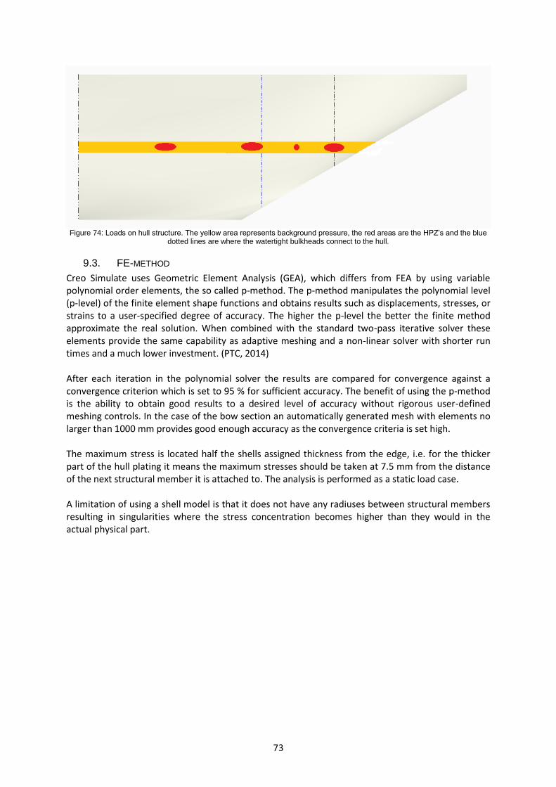
73
Figure 74: Loads on hull structure. The yellow area represents background pressure, the red areas are the HPZ’s and the blue
dotted lines are where the watertight bulkheads connect to the hull.
9.3. FE-METHOD
Creo Simulate uses Geometric Element Analysis (GEA), which differs from FEA by using variable polynomial order elements, the so called p-method. The p-method manipulates the polynomial level (p-level) of the finite element shape functions and obtains results such as displacements, stresses, or strains to a user-specified degree of accuracy. The higher the p-level the better the finite method approximate the real solution. When combined with the standard two-pass iterative solver these elements provide the same capability as adaptive meshing and a non-linear solver with shorter run times and a much lower investment. (PTC, 2014) After each iteration in the polynomial solver the results are compared for convergence against a convergence criterion which is set to 95 % for sufficient accuracy. The benefit of using the p-method is the ability to obtain good results to a desired level of accuracy without rigorous user-defined meshing controls. In the case of the bow section an automatically generated mesh with elements no larger than 1000 mm provides good enough accuracy as the convergence criteria is set high. The maximum stress is located half the shells assigned thickness from the edge, i.e. for the thicker part of the hull plating it means the maximum stresses should be taken at 7.5 mm from the distance of the next structural member it is attached to. The analysis is performed as a static load case. A limitation of using a shell model is that it does not have any radiuses between structural members resulting in singularities where the stress concentration becomes higher than they would in the actual physical part.

74
9.4. RESULTS
All the pictures displaying the results have scale set to 5 to 235 MPa as this is the limit before plastic deformation. The limit for the primary membrane + bending stresses is 235 MPa. This means only the dark red areas have too high stresses. All pictures illustrating result from the analysis show primary membrane and bending stresses combined.
9.4.1. DNV design load
The result from the DNV load case shows that the structure hands the load well. A structural displacement of 2.16 mm for an area that spans 3.4 m is within reasonable limits as seen in Figure 75. Where the main longitudinal girder (girder along ice pressure belt) connects to the bulkheads high stresses occur. One way to decrease the stresses is to increase the hull plating thickness around that area, see Figure 76. However, the stresses are still somewhat too high at the appropriate distance to measure the stresses.
Figure 75: Left: The DNV load and stresses. Right: The displacement caused by the DNV design load.
The results in Figure 76 are not processed at the highest level of accuracy and therefore they are not yielding the same result as in Figure 79.
Figure 76: High stress area caused by the DNV design load. Extra thick (20 mm) hull plating (left) reduces stresses.

75
9.4.2. Load case 1
The extra high pressure zones add on the structure and cause it to deflect more than with the DNV design pressure and also increases stresses markedly. As in the DNV load case the connection between main girder, bulkheads and hull plating has the highest stress concentrations. However, the flange of the main girder is also subjected to high stress as well as the connection between the hull and the web of the main girder at the spot where a HPZ is located. The maximum structural displacement is 5.22 mm, which is quite an increase compared to the DNV design load case. As seen in Figure 78, the problem areas remain from the DNV design load case. The affected areas have increased and have been investigated further, see Figure 79. In Figure 79 the stresses have been reduced locally by cutting of the bottom corner of the girders web where it attaches to the bulkhead.
Figure 77: Left: Load case 1 with three HPZ’s of 7 MPa each. The structure has been stiffened locally to reduce the HPZ
induced loads. Right: Maximum displacement is 5.22 mm.
Figure 78: Close up of problem areas.

76
Figure 79: Left: Load case 1. Right: DNV load case.
The stresses in the main girder and the plating are reduced (less green areas on the left picture in Figure 80) by adding extra stiffening brackets close to the HPZ. In order to reduce computation time only some parts of the structure have been stiffened in this way.
Figure 80: An extra stiffening element is modelled on either side of the high pressure zone (left picture). The extra stiffening
brackets reduces the stresses in the hull plating and main girder and keeps it from “twisting”.

77
9.4.3. Load case 2
The result in the second load case is similar to load case 1. The difference is the increase of area size for stresses above 235 MPa, which is the limit. The maximum displacement of the structure is 7.6 mm and is at the middle of the longest span of the main girder, i.e. at the same spot as in load case 1.
Figure 81: Load case 2: Stresses seen from the inside and outside of the hull.
Figure 82: Left: Load case 2. Right: Load case 1. Note the increase of the red area.

78
9.4.4. Load case 3
The third load case has a single HPZ with a higher pressure than the previous HPZ. If the HPZ is located at the problem areas where the main girder and the bulkheads meet it does not make a significant difference, the stresses in this area increases somewhat as expected. It is clear that the small load causes high stresses at the location and at the connection between main girder and hull. The influence of the HPZ load at the high stress areas is negligible and the stresses at the main girder-bulkhead connection are high in comparison to the DNV load case, see Figure 84.
Figure 83: Left: Load case 2 with stresses seen from the outside. Right: Maximum deflection is 3.15 mm and derives from the
background load on the ice belt.
Figure 84: Left: Load case 3. Right: DNV design load

79
9.5. DISCUSSION ON LOAD ANALYSIS
The magnitude of the stresses in Load Case 2 is quite worrying as they exceed the plastic deformation limit, but as a shell model is a first step in localizing the stresses. The local stresses can be reduced with increasing thicknesses of the hull plate or adding stiffening elements. The next step should be to make a solid model for analysis. Considering the type of model used it could be that the stresses are over estimated. It is also clear that the background pressure affects the structure quite a lot. It exerts a force quite large in comparison to the HPZ and is causing stresses and deflections. By looking at the result (Figure 84) it is clear that the 1.5 MPa background pressure may be too high for the structure to handle without bending too much. The hull seems to handle the DNV design pressure well, specifically when the hull plating is thickened locally. The small red areas in the extra-reinforced case might be due to the shell model and should be checked with a solid model analysis. In load case 1 the stresses are too high in some areas. However, a DNV classed icebreaker can handle ice loads and HPZ’s without major problem although it is designed to cope with a uniform pressure. The reason could be that the HPZ move around rapidly, causing less stresses and deformations, and the static analysis is not a good way of simulating the phenomena. On the other hand, a static load could cause an actual deformation of hull plating and other structural elements, which is commonly seen on icebreakers (and other types of vessels). This suggests that the DNV rules allows for some plastic deformation, and a structure that withstands plastic deformation completely is not obtainable by the rules. That icebreakers can be deformed somewhat could be explained by the fact that the rule based structure could handle the DNV load when it was stiffened, but the background pressure that is (in this case) 50 % higher causes some deformation. The conclusion could be that the DNV design pressure is slightly too low but the structure could handle higher pressures occasionally and only sustain deformation in some areas. As the background pressure is spread over a large area in comparison to the HPZ’s it is quite a substantial force for the structure to cope with and has a large impact on the design. The DNV pressure itself is increasing with increasing vessel size and since the vessel falls outside the DNV rules it could be that the design pressure formulae is not valid in the case of a vessel this size. A larger vessel could have a design pressure higher than the background pressure found in measurements. The 3rd load case behaved as expected. A rather small area with a quite high pressure yields a force that only interacts with the structure locally. It seems that a larger HPZ area has a greater impact on a larger part of the structure than the smaller ones.
9.6. CONCLUSION
In the case of the commuter vessel being designed to meet DNV rules, but falling outside the minimum requirements with regards to machinery output it is not certain that the structure will be strong enough to cope with the stresses and further investigations have to be made. A higher DNV design pressure might lead to a structure better suited to handle the loads as the design pressure is lower than the measured minimum load for larger areas. The main issue seems to be the background pressure being too high, the local pressure zones affect the structure but it is not clear how much. It is not certain that the higher pressures appear as static pressures or is a dynamic load case making it difficult to interpret the results from load case 1 and 2.
80
In order to further investigate the stresses a solid model of the high-stress areas should be analyzed to evaluate the possible stress reduction by using radiuses in connection between structural elements. A fully developed model with relevant stiffening members, decks and more could be used to fully ensure that the commuter vessel can handle ice loads. Different construction materials could be used in order to improve the performance of the structure. Also, the DNV design pressure should be investigated to see if the size of the vessel causes it to become too low. An idea could be to figure out a minimum design pressure and use it for designing a smaller vessel by the rules even though the vessel fall outside the rules. The load cases are based on measurements mainly done in salt or brackish waters making them uncertain to represent a freshwater situation. Tests on actual stresses and pressures should be carried out in freshwater ice to determine actual load cases.
81
10. MAIN DISCUSSION
10.1. Route and ice conditions
The route is located in an area where no exact ice measurements have been registered. It could be that the maximum thickness is higher in some of the bays along the route. If the maximum thickness is somewhat higher in some areas, the vessel would still be able to break the ice but at a lower speed and thus it is not considered to be a significant problem.
10.2. Vessel
Icebreaking requires stronger machinery than running in channels and open water and one way of not having a fleet of commuter vessels with icebreaking capacities running with oversized engines for open water is to limit the icebreaking capacities to a few vessels and use them as icebreakers.
10.3. Icebreaking resistances
When comparing the semi-empirical icebreaking models with the DNV model it is clear that the result is inconsistent. The DNV resistance calculations are based on a modified version of Riska’s formula and the resistance is probably under estimated due to the vessel falling outside the validity range of the design rules. The main drawback of applying Riska’s and Lindqvist’s formula is that they are intended for larger vessels and have not been thoroughly evaluated for smaller vessels. The reason they are used anyways is that there are no other methods available for estimating resistances for small vessels other than testing. On the other hand, Lindqvist’s model has been used for smaller vessels and the result is consistent with measurements ((Lindqvist, 1989) & (Biao, Riska, & Moan, 2011)). The main drawback of Riska’s formula is that it does not take the freshwater ice properties into account, which makes the formula unsuitable for the commuter vessel. Further this implies that the DNV icebreaking resistance is not suitable for freshwater conditions. It is noticeable that the bow angles have significant impact on the resistance given by the Lindqvist and Riska models, both in icebreaking and running in brash ice. The magnitude of the resistance is however changing with varying bow angle combinations. In general both methods point towards that a low stem angle reduces resistance, which is in line with the ice having a lower flexural strength than crushing strength. Thus, bending failure comes before crushing failure and by designing the bow to “slide” on top of the ice and transfer force downwards instead of crushing the ice head on yields less resistance. A bow optimized for icebreaking or channel resistance might increase the open water resistance. It is also clear that the speed is an important parameter for the resistance. It is worth considering which speed is required when breaking the ice as the operational profile suggests the icebreaking activities are only a few percent of the operational time. Depending on the operational profile the vessel should be investigated for brash ice resistance more fully. It is worth comparing breaking new channels more often or running in channels until they are filled with more brash ice, requiring larger propulsion machinery for the vessels that only run in channels and not break ice.
10.4. Structural design and its weaknesses
The DNV design ice pressure is differing dependent on the size and hierarchy of the structural member that is being designed. A larger structural member results in a larger load area, which means that the dimensioning design pressure decreases. When applying the loads as in 9.2, one must keep in mind that the most critical design load should be applied. This means that the design load for plating is the design load for which the structure is investigated. A second design iteration should aim to refine the design loads for each and every member in the structure, so that all parts in the

82
structure are dimensioned individually. As for now, the longitudinal ice girder is dimensioned to carry the design pressure it is exposed to in its largest span. The structure is in this case not conservative and should instead be dimensioned to hold for the design pressure appearing in the shortest span, since it is of larger magnitude. This might be one of the reasons to why the structural design from DNV seems to be a bit weak. The first design loop in the iterative development process is complete. Main parameters stated here are recurrent in the overall work and used as a foundation for the rest of the conclusions in this report.
10.5. Load analysis
The load cases are based on measurement data and DNV design pressure. The minimum measured pressure for a line load is 1.5 MPa. If this is correct for the freshwater ice in Lake Mälaren, the DNV design load of 1 MPa gives a too weak structure to handle the minimum measured loads. However, the design rules gave a structure that was coping well with the pressure it was supposed to handle. The result from the DNV load case implies that the design rule works but the minimum design pressure is too low. The high pressure zones in Load case 2 yields higher stresses on the structure than the structure can handle. However, the analysis was static and a dynamic load could have a smaller effect on the structure and thus a static load case could overestimate the actual impact of an HPZ. The smaller HPZ’s or the zones with lower pressure affects the structure locally. The main area that is affected here is the hull plating, which means there can be some plastic deformation in this area but it is not dangerous for the structure. It should be noted that the structural analysis was performed using a shell model. A shell model does not have any radiuses and thus singularities and stress concentrations can appear to be more severe than in a solid model. Some stresses seen in the figures from the analysis may therefore be reduced in a solid model. This implies that areas of uncertainty should be modeled as solids before a conclusion can be made.

83
11. MAIN CONCLUSION Breaking ice is considered an exceptional operational condition, meaning that the demand for speed according to the operational profile is left aside. However, an assumption that the vessel should be able to make a speed of 5 knots in these conditions is made.
It is clear that the most critical operational condition demands a minimum engine power output equal to approximately 400 kW as seen in Figure 15, which is well within capacity range for chosen engine arrangement. The open water resistance is illustrated in Figure 11 and estimated to approximately 300 kW for the service speed of 12 knots. It is hereby clear when looking at the operational profile that the minimum engine output can be lowered by 25 % if the decision is made to reduce the operational time with as little as 2 %. If a decision like this would be made, it implies that another engine arrangement perhaps would be more suitable and that the year around operational demand might be questionable from a cost perspective.
The ice breaking and brash ice resistance models can serve as an estimation tool at the first design stage evaluating the resistance that the vessel could encounter. The models are however not fully tested for small vessels or freshwater ice conditions. The design of the bow has a large impact on the total resistance of the vessel. As the Riska model does not take freshwater ice properties into account it is not suitable to be used on the commuter vessel. Additionally this implies that the DNV icebreaking resistance is not suitable for freshwater conditions either. Further tests have to be executed to verify that the Lindqvist resistance formula is suited for evaluating small vessels in freshwater ice conditions.
The hull shape fulfills the main criteria. It has been developed through an iterative process involving open water resistance and hydrostatic stability calculations, while in the same time controlling main deck measurements, displacement and bow shape angles.
It is not certain the structure will be strong enough to cope with the stresses and further investigations have to be made. The DNV design load of 1 MPa gives a too weak structure to handle the minimum measured loads. However, the design rules gave a structure that was coping well with the pressure it was supposed to handle. The result from the DNV load case implies that the design rule works but the minimum design pressure is too low. A more detailed tuning of the parameters used for calculating the DNV rule based minimum power requirement (5.3.3) could open up for a widened validity span of the resistance calculations. Connecting these calculations to the design ice pressure estimation (5.5.2) could then result in a more reliable result for vessels that today falls outside the validity span.
84
12. MAIN FUTURE WORK The design of the vessel is only in its first stage and needs to be developed further to work as a complete foundation for more detailed investigations. A more detailed general arrangement is needed to generate stability calculations and design pressures with high accuracy. Investigating operational cost is also subject for future work. A holistic picture of how results from DNV design load calculations vary and deviate from analytical results depending on ship size can be obtained through a statistical approach, by comparing a large number of vessels with varying dimensions. In order to investigate if the DNV design pressure should have a minimum limit of 1.5 MPa, which measurements suggests, tests in freshwater ice have to be performed to verify the minimum ice load. The minimum measured ice load in freshwater is then used to evaluate the DNV design pressure by performing an FE analysis on a DNV designed vessel in the same way as presented in chapter 9. Further, the Lindqvist icebreaking resistance formula should be tested for fresh water ice conditions on vessels the same size as the commuter ferry. Thus the size of the vessel and the freshwater ice conditions are investigated. It is also of importance to verify the flexural strength of the ice to further investigate the resistance formula. In short, trials in freshwater ice have to be carried out to ensure the resistances can be estimated correctly. If resistance models can be verified and used, an optimal vessel can be found based on the operational profile.

85
REFERENCES ABS, A. B. (2005). ABS GUIDANCE NOTES ON ICE CLASS. Houston. Biao, S., Riska, K., & Moan, T. (2011). Numerical study of ice-induced loads on ship hulls. Marine
Structures, 24, 132-152. Couser, D. P., Wellicome, D. J., & Molland, D. A. (1998). An improved method for the theoretical
prediction of the wave resistance of transom-stern hulls using a slender body approach. Southampton, U.K.: Department of Ship Science, University of Southampton.
Dempsey, J., Palmer, A., & Sodhi, D. (2001). High pressure zone formation during compresive ice
failure. Engineering Fracture Mechanics, 68, 1961-1974. Det Norske Veritas. (2014, January 1). DNV. Retrieved March 31, 2014, from DNV service documents:
https://exchange.dnv.com/servicedocuments/dnv Det Norske Veritas. (DNV service documents, 2014 January). DNV. Retrieved 2014 March, 1, from
http://exchange.dnv.com/servicedocuments/dnv DNV. (2012). RULES FOR CLASSIFICATION OF Ships Pt3 Ch2 Sec2 Materials B200-B203. Hövik: Det
Norske Veritas. Formsys. (2014). Hydromax version 11. Formsys. Formsys. (2014). Maxsurf version 11. Formsys. Fransson, L. (2009). ICE HANDBOOK FOR ENGINEERS (Version 1.2 ed.). Luleå: Luleå University of
Technology, Institutionen för samhällsbyggnad. FSICR. (2014). Sjöfartsverket. Retrieved March 17, 2014, from
http://www.sjofartsverket.se/pages/40584/b100_1.pdf Google. (n.d.). Google Maps. Retrieved January 5, 2014, from https://maps.google.se Jastram manuevring competence. (2014). Jastram transverse thrusters. Retrieved January 30, 2014,
from http://www.jastram.net/transverse_thrusters.0.html Johnston, M., Croasdle, K., & Jordaan, I. (1998). Localized pressures during ice-structure interaction:
relevance to design criteria. Cold Regions Science and Technology, 27, 10. Jordaan, I. (2001). Mechanics of ice-structure interaction. Engineering Fracture Mechanics, 68, 123-
1960. Karlsson, T. (2013). Förslag på försök med nya pendelbåtslinjer på Stockholms inre vatten. Stockholm:
AB Stockholms Lokaltrafik. Kujala, P. (1994). On the Statistics of Ice Loads on Ship Hull in the Baltic. Helsinki: ACTA
POLYTECHNICA SCANDINAVIA, MECHANICAL ENGINEERING SERIES No. 116.

86
Lindqvist, G. (1989). A staright forward method for calculations of ice resistance of ships. International Conference on Port and Ocean Engineering under Arctic Conditions, (pp. 722-735). Luleå.
Lubbad, R., & Løset, S. (2011). A numerical model for real-time simulation of ship-ice interaction. Cold
Regions Science and Technology(65), 111-127. Malmsten, G. (2014, February 3). Trafikchef, Trafikförvaltningen. Maritime Journal. (2005, May 1). Maritime Journal. Retrieved 03 31, 2014, from HADAG Gets -
Seventh Type 2000 and Plans More: http://www.maritimejournal.com/news101/industry-news/hadag_gets_seventh_type_2000_and_plans_more
Maritime Journal. (2005). www.maritimejournal.com. Retrieved february 27, 2013, from
http://www.maritimejournal.com/news101/industry-news/hadag_gets_seventh_type_2000_and_plans_more
Martio, J. (2007). Numerical Simultaion of Vessel's Manoeuvring Performance in Uniform Ice. Helsinki:
Aalto University (Helsinki University of Technology), Ship Laboratory. Masterson, D. M., & Frederking, R. (1992). Local contact pressures in ship/ice and structure/ice
ineractions. Cold Regiions Science and Technology, 21, 169-185. Masterson, D., Frederking, R., Wright, B., Kärnä, T., & Maddock, W. (2007). A revised ice pressure-aea
curve. Dalian: 19th International Conf. on Port and Ocean Engineering under Arctic Conditions.
Mellor, M. (1980). Ship Resistance in Thick Brash Ice. Cold Regions Science and Technology, 305-321. NordicPhotos. (2011). NordicPhotos. Retrieved March 24, 2014, from http://www.nordicphotos.com Palmbeck, J. (2013). Utredning om båtpendling i Stockholm. Stockholm: Trafikförvaltningen,
Stockholms läns landsting. Palmer, A., Dempsey, J., & D.M., M. (2009). A revised ice pressure-area curve and a fracture
mechanics explanation. Cold Regions Science and Technology, 56, 73-76. Panoramio. (n.d.). Panoramio. Retrieved March 24, 2014, from
http://www.panoramio.com/photo/24947600 Petrovic, J. (2003). Review: Mechanical properties of ice and snow. Journal of Materials Science, 38,
1-6. PTC. (2014). PTC. Retrieved May 02, 2014, from PTC Creo: http://www.ptc.com/product/creo/ Rindeskär, M. (2014, February 3). Technical Supervisor. Riska, K., Wilhelmson, M., Englud, K., & Leiviskä, T. (1997). Performance of merchant vessels in the
Baltic. Finnish Maritimie Administration and Swedish Administartion of Shipping and Navigation.

87
Rolls Royce. (2014). www.rolls-royce.com. Retrieved February 20, 2014, from http://www.rolls-royce.com/Images/RR-B_Propulsion_0612_singlepages_LR10_250512_tcm92-8664.pdf
Sjöfartsverket. (2006). www.sjofartsverket.se. Retrieved March 24, 2014, from
http://www.sjofartsverket.se/upload/SJOFS/2006_1.pdf Sjöfartsverket. (2010). www.sjofartsverket.se. Retrieved February 27, 2014, from
http://www.sjofartsverket.se/funktionshinder/ SMHI. (2011a). Retrieved March 24, 2014, from http://www.smhi.se/en/theme/sea-ice-1.11198 SMHI. (2011b). Retrieved February 27, 2014, from
http://www.smhi.se/oceanografi/istjanst/produkter/arkiv/maxis/maxis_2011.pdf SMHI. (2014). Retrieved March 26, 2014, from http://www.smhi.se/klimatdata/oceanografi/havsis SSPA. (2001). Biogasfärja. Stadsledningskontoret, Lokala investeringsprogrammet. Stockholm: LIP-
kansliet. Suyuthi, A., Leira, B., & Riska, K. (2012). Short term extreme statistics of local ice loads on ship hulls.
Cold Regions Science and Technology, 82, 130-143. Swedish Transport Agency. (2013, 12 19).
https://www.transportstyrelsen.se/tsfs/TSFS_2009_114.pdf. Retrieved 4 2, 2014, from https://www.transportstyrelsen.se/sv/Sjofart/Fartyg/Fartygskonstruktion/Skrovkonstruktion-och-dimensionering/.
Timco, G. W., & O'Brien, S. (1994). Flexural strength equation for sea ice. Cold Regions Science and
Technology, 22, 285-298. Timco, G. W., & Sudom, D. (2013). Revisiting the Sanderson pressure-area curve: Defining
parameters that influence ice pressure. Cold Regions Science and Technology, 95, 53-66. Timco, G. W., & Weeks, W. F. (2010). A review of the engineering properties of sea ice. Cold Regions
Science and Technology, 60, 107-129. TRAFI. (2011). GUIDELINES FOR THE APPLICATION OF THE FINNISH-SWEDISH ICE CLASS RULES.
Helsinki. UAA, C. o. (2014, April 4). University of Alaska Anchorage, College of Engineering. Retrieved May 13,
2014, from Properties of Ice II: http://www.google.se/url?sa=t&rct=j&q=&esrc=s&source=web&cd=3&ved=0CEsQFjAC&url=http%3A%2F%2Fsoe.uaa.alaska.edu%2Fsoe%2Fcourses%2Fce334%2FStudent_Share%2FLecture%2520Notes%2FLect23Ice-2.ppt&ei=EhByU-dlyL3KA7SkgegC&usg=AFQjCNFz7n-B2m8L-AqAs5sDRANVGHsFBQ&si
Volvo Penta. (2013). www.volvopenta.com. Retrieved February 20, 2014, from
http://www.volvopenta.com/volvopenta/na/en-us/MarineCommercialEngines/Inboard/engine_range/Pages/d13_mh.aspx