400 Commonwealth Drive, Warrendale, PA 15096-0001 U.S.A. Tel: (724) 776-4841 Fax: (724) 776-5760 Web: www.sae.org

SAE TECHNICALPAPER SERIES 2004-01-0898

Identification and Speed Control of SI Engine

Joško Deur, Vladimir Ivanovi and Danijel PavkoviUniversity of Zagreb, Croatia

Martin JanszFord Motor Company Ltd., UK

Reprinted From: Electronic Engine Controls 2004(SP-1822)

2004 SAE World CongressDetroit, MichiganMarch 8-11, 2004

for Idle Operating Mode

All rights reserved. No part of this publication may be reproduced, stored in a retrieval system, ortransmitted, in any form or by any means, electronic, mechanical, photocopying, recording, or otherwise,without the prior written permission of SAE.

For permission and licensing requests contact:

SAE Permissions400 Commonwealth DriveWarrendale, PA 15096-0001-USAEmail: permissions@sae.orgFax: 724-772-4891Tel: 724-772-4028

For multiple print copies contact:

SAE Customer ServiceTel: 877-606-7323 (inside USA and Canada)Tel: 724-776-4970 (outside USA)Fax: 724-776-1615Email: CustomerService@sae.org

ISBN 0-7680-1319-4Copyright © 2004 SAE International

Positions and opinions advanced in this paper are those of the author(s) and not necessarily those of SAE.The author is solely responsible for the content of the paper. A process is available by which discussionswill be printed with the paper if it is published in SAE Transactions.

Persons wishing to submit papers to be considered for presentation or publication by SAE should send themanuscript or a 300 word abstract of a proposed manuscript to: Secretary, Engineering Meetings Board, SAE.

Printed in USA

2004-01-0898

Identification and Speed Control of SI Engine for Idle Operating Mode

Joško Deur, Vladimir Ivanović ć University of Zagreb, Croatia

Martin Jansz Ford Motor Company Ltd., UK

ABSTRACT

A nonlinear mean value engine model has been identified by using engine static maps. The model is linearized, simplified, and analyzed for the idle speed operating mode. Least-squares estimation of different types of input-output linear model are considered, with the aim to find a proper identification technique in the presence of significant speed perturbations of weakly excited engine. An analytical design method of tuning the PI and PID idle speed controllers is proposed. The method is based on the damping optimum criterion. Design of a more advanced, polynomial speed controller is also presented. The controllers are experimentally verified and compared.

INTRODUCTION

Effective idle speed control of SI engines is needed to fulfill the increasing requirements of improved fuel economy, reduced emissions, guaranteed combustion stability, and good NVH quality. The aim of idle speed controller is to keep the idle engine speed as close as possible to a reference value (typically 750 rpm), regardless of changes of engine load due to the engagement of accessories such as air conditioning, alternator, and power steering. More effective load disturbance rejection provides the application of lower reference idle speed without the risk of engine stalling, and thus leads to lower fuel consumption and reduced emissions.

Idle speed control system design includes standard steps such as modeling of nonlinear plant (engine) dynamics, experimental identification, controller design, controller implementation, and experimental verification. A comprehensive survey of modeling and control methodologies for idle speed control is given in [1]. The engine dynamics is commonly described by a nonlinear mean value engine model (see e.g. [2]). The model is linearized [3] for the idle operating region with the aim to provide application of many well-known and effective

linear control system design and analysis techniques. In order to avoid model parameterization and linearization, modern experimental identification techniques can be used to obtain the linear model directly [4,5]. The PID controller (or its variants such as I or PI controller) is commonly used in the automotive practice to control the engine speed through the throttle angle channel. It is usually extended by a proportional feedback which acts through the fast spark advance channel, in order to improve the disturbance rejection performance. Further disturbance rejection improvements can be reached by implementing a feedforward disturbance compensator based on the measured, reconstructed, or estimated load torque signal. More advanced linear and nonlinear, feedback and feedforward control strategies are discussed in [1] and references therein.

Experimental identification of the linear input-output engine dynamics is usually based on the relatively simple discrete-time models, such as output-error or ARX model [4]. Since the idle speed engine dynamics varies with the engine load operating point, a nonlinear ARX model (NARX model) is proposed in [5]. The simple input output models can accurately capture the engine dynamics only in the case of good signal-to-noise ratio. This implies that the perturbations of the engine throttle angle (or spark advance) should be relatively large, especially for low power engines that include larger engine speed "noise". The large throttle angle perturbations results in a large engine speed variance, which may be inconvenient in practice, particularly for on-line identification. Therefore, it is generally convenient to provide an accurate engine dynamics identification with a relatively low variance of the throttle angle. This can be achieved by using more complex input-output models, such as ARMAX or Box-Jenkins model, which include better noise description. In order to analyze benefits of the use of complex input-output models, a comparative study of experimental identification of a V2 engine is presented in this paper.

The PI/PID idle speed controller parameters are usually tuned by trial-and-error method, or by a numerical or

Copyright © 2004 SAE International

and Danijel Pavkovi

semi-numerical method (e.g. numerical optimization). However, it is generally more convenient to use practical and optimal analytical relations for the controller parameters, which would be based on the physical process parameters such as manifold time constant or combustion delay. Such an analytical approach based on the damping optimum design method [6,7] is proposed in the paper.

The paper also presents the design of the polynomial controller [8], which can be regarded as a full-order linear discrete-time controller with an implicit observer. Such a controller was previously successfully applied for speed control of an electrical drive with compliant transmission [9]. Since the polynomial controller controls all modes of the process dynamics (full-order controller), it should provide better control performance than the PI/PID controller. At the same time, it may be more effective than the reduced-order state controller proposed in [10]. The designed controllers are experimentally verified and compared on an experimental setup of a 14 HP V2 SI engine with an electronic throttle included.

ENGINE MODEL

NONLINEAR MEAN VALUE ENGINE MODEL

The mean value SI engine model with the isothermal manifold heat transfer can be described by the block diagram shown in Fig. 1a [2,3,11]. The model includes two states (the manifold pressure p and the engine speed ω), four nonlinear static maps, and a pure combustion delay Td. The model input is the throttle angle θ. The spark advance (δ) channel is not used in most of the paper, because it cannot be controlled on the particular engine. The air/fuel ratio is not used for the same reason.

The model static maps can be expressed by semi-empirical analytical functions, as shown in [2].

Alternatively, they can be given in the form of experimentally recorded look-up tables. In order to facilitate the procedure of recording the maps, it is convenient to lump the produced engine torque map Mu and the loss torque map Ml to a single torque map M(Wo, ω), as shown in Fig. 1b. [11]. This simplification is based on the following two conditions which are normally satisfied:

1. Changes of the engine speed ω inside the combustion delay interval Td are negligible.

2. The torque production gain through the path p→Mu is much higher than the pumping loss gain of the path p→Ml.

The maps of the simplified model in Fig. 1b can be recorded by standard engine dynamometer tests (see e.g. [11]).

LINEARIZED MODEL

The nonlinear mean value engine model, given in Fig. 1a, can be transformed to the linearized form shown in Fig. 2a [3]. The linearization process, including the equations for the linearized model gains, is elaborated in [3]. The linearized model from Fig. 2a can conveniently be transformed to the model given in Fig. 2b. Based on the assumptions 1 and 2 above, the model can be simplified to the standard linear engine model form shown in Fig. 3a [12] (cf. [13]). The expressions for the model parameters are given in Appendix A.

The model can be further simplified if the following additional assumption is satisfied:

3. The manifold dynamics is much faster than the rotational dynamics.

In this case, the pumping feedback through the gain Kp together with a pumping feedback term included in the transfer function G*

mech(s) (see the path through gain N7 in Fig. 2b) may be neglected, thus resulting in the model shown in Fig. 3b. Note that the rotational dynamics transfer functions of the models in Figs. 3a and 3b are not the same (Appendix A). Gmech(s) is the real transfer function of the rotational dynamics, while G*

mech(s) is a fictitious rotational dynamics transfer function which includes the pumping feedback contribution.

And finally, the transfer function Gmech(s) may

Fig. 1. Block diagram of engine model: original form (a) and simplified form (b).

be simplified to the operating point-independent transfer function 1 / Is (Fig. 3c) if the following assumption is satisfied:

4. The closed-loop control system is much faster than the rotational dynamics.

The assumptions 1-4 relate to the following conditions, respectively:

1. Td << Tmech

2. 5231 >>+

120NNN

RTVP d

3. Tm << Tmech

4. Te << Tmech

where Te is the equivalent time constant of the closed-loop system (see below).

ANALYSIS OF LINEARIZED MODEL

It has been reported in [3] that the conditions 1-3 are indeed well satisfied for the full operating range of the 1.275L SI engine from [2]. The time constants of the original linearized model (Fig. 2a) and the simplified model (Fig. 3b) were found to differ for less than 20% (or less than 10% for ω > 2000 rpm). This implies that the simple aperiodic model in Fig. 3b may be a good representative of the engine dynamics for controls. However, it was shown in [13] that the engine dynamics can be oscillatory under the idle conditions. The oscillatory behavior is caused by the coupling between the manifold and rotational dynamics, which is realized through the pumping feedback in the model in Fig. 3a. This would mean that the pumping feedback can be emphasized for one engine and negligible for another one.

Algebraic and numerical analyses in [12] show that the engine model from Fig. 3a tends to the oscillatory behavior if (absolute values of) its time constants (Tm, Td, and T*

mech) are closer to each other, and if the open-loop gain KmKtK*

mechKp is higher. This result is illustrated by the comparative simulation results in Fig. 4. The engine model with the original parameters from [2] exhibits aperiodic behavior (Fig. 4a), and the pumping feedback may be neglected (the simple model in Fig. 3b is quite accurate). This is the consequence of relatively

a

b Fig. 2. Block diagram of linearized mean value engine model.

a

b

c Fig. 3. Illustration of simplification of linearized engine model.

slow rotational dynamics (i.e. large T*mech) and

relatively fast manifold dynamics (i.e. small Tm). According to [12] (see also Appendix A), T*

mech is large due to apparently unrealistically high engine inertia I = 0.48 kgm2 (probably due to engine dynamometer inertia included), and Tm is low due to the relatively low manifold volume-to-engine displacement ratio V / Vd = 0.5 (note that V / Vd is often greater than 2 for modern SI engines). Fig. 4b illustrates that the engine model with four-fold decreased inertia I and five-fold increased ratio V / Vd exhibits oscillatory behavior. In this case, the simple model in Fig. 3b cannot provide an accurate response.

The above analysis shows that the simple model from Fig. 3b should be viewed with skepticism for idle operations. On the other hand, it should be accurate at large speeds for many engines (note that Tm and 1/T*

mech decrease with speed increase [3]).

The simulation results in Fig. 4 reveal additional two interesting effects:

• The final (steady-state) value of the manifold pressure response is lower than the initial pressure value. This is the consequence of negative "mechanical" gain K*

mech. Note that the “mechanical” time constant T*

mech is also negative, i.e. the "equivalent" rotational dynamics described by G*

mech(s) is unstable. The effect only occurs for low-speed (idle) operating mode and constant load torque (Mb ≠ f(ω)) (see [12] for more details).

• Unlike the aperiodic manifold pressure response p of the simple model in Fig. 3b, the non-simplified model response shows a lead-lag behavior (Fig. 4a). However, the initial high-frequency parts of both responses are very similar for the aperiodic model. Thus, the "real", lead-lag pressure response may be used to graphically determine the manifold time constant Tm, as illustrated in Fig. 4a.

Fig. 4 also demonstrates that the models in Figs. 2 and 3a have very similar behavior for both sets of model parameters, which justifies the assumptions 1 and 2 above.

PROCESS IDENTIFICATION

APPROACH BASED ON ENGINE MAPS

Since the parameters of linear parts of the simplified mean value engine model in Fig. 1b are known physical constants, the model identification relates to obtaining the nonlinear engine static maps. These maps have been recorded on an experimental setup of a 14 HP 0.46L V2 Briggs and Stratton SI engine [14] by executing a series of steady-state engine dynamometer runs over the whole engine operating region. The recorded maps are shown in Fig. 5.

a

b

Fig. 4. Linear engine model responses with respect to small step change of throttle position at 0.1 s, for two sets of engine parameters.

Fig. 5. Recorded engine model maps.

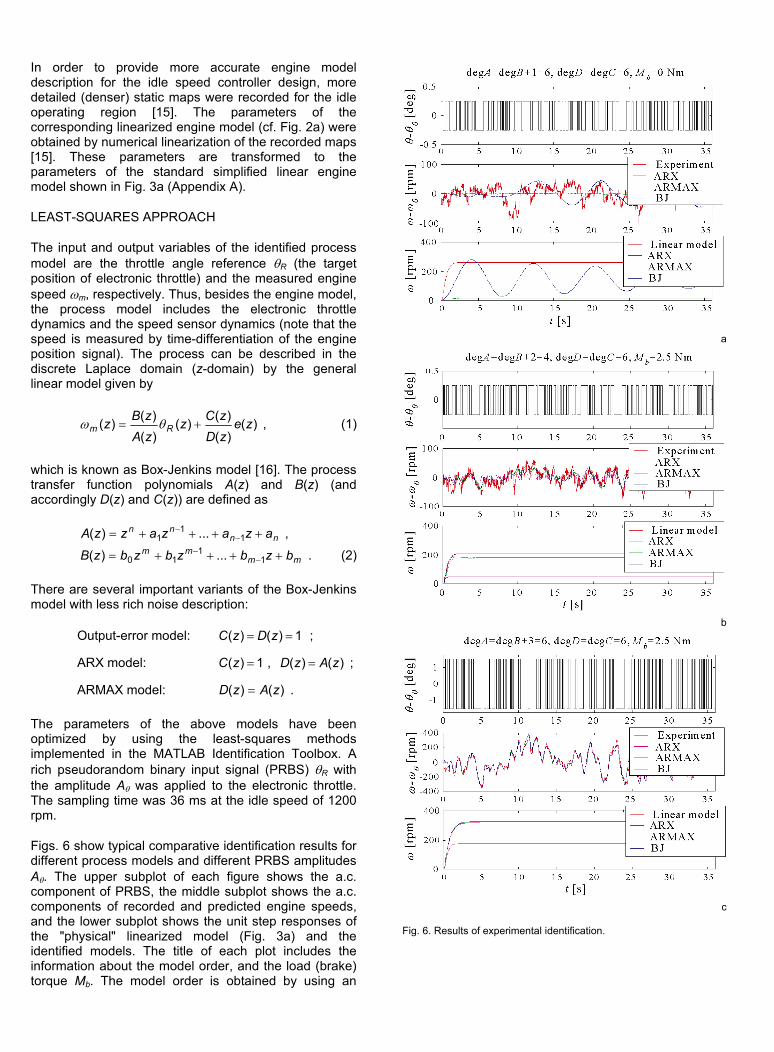
In order to provide more accurate engine model description for the idle speed controller design, more detailed (denser) static maps were recorded for the idle operating region [15]. The parameters of the corresponding linearized engine model (cf. Fig. 2a) were obtained by numerical linearization of the recorded maps [15]. These parameters are transformed to the parameters of the standard simplified linear engine model shown in Fig. 3a (Appendix A).

LEAST-SQUARES APPROACH

The input and output variables of the identified process model are the throttle angle reference θR (the target position of electronic throttle) and the measured engine speed ωm, respectively. Thus, besides the engine model, the process model includes the electronic throttle dynamics and the speed sensor dynamics (note that the speed is measured by time-differentiation of the engine position signal). The process can be described in the discrete Laplace domain (z-domain) by the general linear model given by

)()()()(

)()()( ze

zDzCz

zAzBz Rm += θω , (1)

which is known as Box-Jenkins model [16]. The process transfer function polynomials A(z) and B(z) (and accordingly D(z) and C(z)) are defined as

nnnn azazazzA ++++= −

−1

11 ...)( ,

mmmm bzbzbzbzB ++++= −

−1

110 ...)( . (2)

There are several important variants of the Box-Jenkins model with less rich noise description:

Output-error model: 1)()( == zDzC ;

ARX model: )()( , 1)( zAzDzC == ;

ARMAX model: )()( zAzD = .

The parameters of the above models have been optimized by using the least-squares methods implemented in the MATLAB Identification Toolbox. A rich pseudorandom binary input signal (PRBS) θR with the amplitude Aθ was applied to the electronic throttle. The sampling time was 36 ms at the idle speed of 1200 rpm.

Figs. 6 show typical comparative identification results for different process models and different PRBS amplitudes Aθ. The upper subplot of each figure shows the a.c. component of PRBS, the middle subplot shows the a.c. components of recorded and predicted engine speeds, and the lower subplot shows the unit step responses of the "physical" linearized model (Fig. 3a) and the identified models. The title of each plot includes the information about the model order, and the load (brake) torque Mb. The model order is obtained by using an

a

b

c

Fig. 6. Results of experimental identification.

automated model selection procedure applied to the Box-Jenkins model.

The following observations can be drawn from the identification results given in Fig. 6:

• The identification results are bad for low PRBS amplitude Aθ = 0.25o and zero load torque (Fig. 6a). All the identified models are not capable to reproduce the recorded engine speed trace and predict the correct unit step response. This is the consequence of "irregular" form and large variance of the speed of the unload engine for θR ≈ const. These, primarily stochastic, engine speed variations are completely missed by the ARX and ARMAX models due to the lack of good noise description. The identification results at Mb=0 become reasonable for the PRBS amplitudes Aθ > 0.6o (no figure).

• Identification results are much better for larger engine load torque (Fig. 6b, Mb = 2.5 Nm which equals 10% of the rated load and 50% of the maximum expected idle load). The Box-Jenkins model predicts accurate engine behavior even for low PRBS amplitude Aθ = 0.25o. Similar (though somewhat worse) behavior is observed for the ARMAX model. However, the simpler ARX model does not give good results, due to poor noise description.

• In the case of sufficiently large PRBS amplitude (Aθ = 1.5o), the signal/noise ratio becomes large, and all the considered models predict similar accurate speed response of loaded engine (Fig. 6c). However, it is important to note that the large PRBS amplitude causes very large speed variations (±400 rpm in Fig. 6c compared with ±50 rpm in Fig. 6b), which may be inconvenient for practical identification tests, especially for possible on-line identifications (e.g. for adaptive controls). Also, due to the large variations of the input and output signals, the system exits from the linear operating region, which affects the accuracy of the identified model for the particular operating point (the lowest plot of Fig. 6c).

DESIGN OF IDLE SPEED CONTROLLER

PI/PID CONTROLLER

Fig. 7 shows the block diagram of the equivalent continues-time idle speed control system with a PI/PID controller and an optional spark advance-channel P controller. The linear engine model is taken from Fig. 3a, where the pure combustion delay exp(-Tds) is approximated by the transfer function 1 / (Tds + 1) (zero-order Padé approximation). The engine model transfer function is given by (with KRδ=0, no spark advance control):

012

23

3)()()(

eeee

ee

asasasaK

sssG

+++==

θ

ω , (3)

with

*mechtme KKKK =

pee KKa += 10

*1 mechdme TTTa ++=

mmechmechddme TTTTTTa **2 ++=

*3 mechdme TTTa = .

The relatively fast, inner electronic throttle control loop is approximately described by an equivalent first-order lag term with the time constant Tθ. The equivalent time constants of the sampler + zero-order-hold element and the speed measurement term (based on position differentiation) are equal to T / 2 (T - sampling time; see e.g. [7]), so that these two parasitic terms are described by the lag term with the time constant T. The measured speed signal may be filtered by a low-pass filter with the time constant TFω. The time constants Tθ, T, and TFω have relatively small values (typically 20 ms) when compared to the engine time constants Tm, Td, and T*

mech. Thus, they may be treated as parasitic time constants. The three process parasitic terms may be approximated by a single first-order lag term (see e.g. [7]):

ωθ FTTTTsT

sG ++=+

= ΣΣ

Σ , 1

1)( . (4)

In this way, the original seventh-order closed-loop model (Fig. 7) is reduced to the fifth-order model, which simplifies the design procedure and equations for the controller parameters.

The PID controller parameters are determined according to the damping optimum [6,7]. This is a simple and powerful pole-placement-like analytical method of design of linear continuous-time systems of arbitrary order. The most important characteristic of the method is the possibility of analytical optimization of parameters of a reduced-order controller. The method is based on the closed-loop characteristic polynomial given in the form

1)( 222

333

22

23

12 +++++= −− sTsTDsTDDsTDDDsN eee

nnen

nn KL (5)

where Te is the equivalent time constant, and D2,

D3,...,Dn are the characteristic ratios. In the optimal case D2 = D3 = ... = Dn = 0.5 [6,7], the closed-loop system of any order n has a quasi-aperiodic step response with an overshoot of approx. 6% and the rise time of approx. 1.8Te. In the case of reduced-order controller, only the dominant characteristic ratios D2, D3,...,Dr (r < n) are set to the optimal value of 0.5.

Based on the control system block diagram (Fig. 7; TD = 0 for PI controller) and Eqs. (3) and (4), the closed-loop transfer function can be derived. Equating the coefficients of the closed-loop characteristic polynomial with the corresponding coefficients of the damping optimum polynomial (5), and rearranging yields the final eqations for the PI/PID controller parameters:

PI controller:

−+= Σ 11

20

2

1

ee

e

e

eR

TDTa

TDa

KK ,

eR

e

eI

KKa

TT

01+= ,

10

21

32min

1

ee

eee

aTaaTa

DDT

+

+=

Σ

Σ ; (6)

PID controller:

−

+= Σ

02223

211e

e

ee

eR a

TDDaTa

KK ,

eR

e

eI

KKa

TT

01+= ,

+= Σ

Σ TaaTDDaTa

KKT ee

e

ee

eRD 01

3

211 --2

,

21

32

234min

1

ee

eee

aTaaTa

DDDT

+

+=

Σ

Σ . (7)

In order to provide fast and well-damped response, the characteristic ratios D2, D3, and D4 in Eqs. (6) and (7) should be set to the optimal value of 0.5, and the equivalent time constant Te should be equal or greater than Temin. Increase of Te improves the control system robustness and decrease the noise sensitivity, but, in turn, results in slower response and less efficient disturbance rejection.

The above analytical design method can be applied to the case of combined throttle angle + spark advance control (Appendix B).

POLYNOMIAL CONTROLLER

The engine speed control system with the polynomial controller is shown in Fig. 8. The polynomial controller is a general discrete-time linear controller with an implicit state observer [8]. It controls all process states (full-order controller). The controller is described as:

)()()()(

)()()( z

zPzQz

zPzSz mRR ωωθ −= , (8a)

which is implemented in the form of two-input difference equation. Note that the measured speed filter is not necessary now, because the implicit observer has low-pass filtering properties. The steady-state accuracy of the control system with respect to load torque is provided by including an integral term into the speed controller:

)()1()( ' zPzzP −= . (8b)

The discrete-time process transfer function is given by

)()(

)()()(

zAzB

zzzG

R

mp ==

θ

ω . (9)

Fig. 7. Block diagram of idle speed control system with PID controller (PI controller if TD = 0).

It can be obtained by direct discrete-time process identification (see Eq. (1)), or by applying the Z-transform to the continuous-time form of the process model given in Fig. 7. In the latter case, the process transfer function reads

)()()()(1)1(11)(

21

zAzBsGsG

sz

zz

TzG ep =

Ζ−= −θ

- , (10)

51degdeg =+= BA . (11)

Since, the polynomial controller can control all process modes, it is necessary to provide an accurate process description. In this sense, it is convenient to approximate the combustion delay term exp(-Tds) with the transfer frunction (1 – 0.5Tds) / (1 + 0.5Tds) (first-order Padé approximation) which gives the engine transfer function Ge(s) given in Appendix C.

Combining Eqs. (8) and (9) yields the closed loop transfer function

)()()()(

)()()()()()(

)()(

)(0

0

zAzA

zBzA

zQzBzPzAzSzB

zz

zGM

M

R

mcl =

+==

ω

ω (12)

which is equated with the model transfer function [8]

)()(

)(zAzB

zGM

MM = , ABA MM deg1degdeg =+= , (13)

expanded in its numerator and denominator with the so-called observer polynomial Ao(z). The polynomials A(z), AM(z), Ao(z), and P(z) are monic polynomials (the coefficient of the highest power is equal to one).

The solution of Eq. (12) is given by [8,9]:

)()1()1(

)( zAB

AzS o

M= , (14)

)()()()()()( zAzAzQzBzPzA Mo=+ , (15)

where

AASQPP degdegdegdeg1'degdeg 0 ====+= . (16)

The Diophantine equation (15) is transformed into a system of linear algebraic equations, which yields the solution for the coefficients of P(z) and Q(z) [8].

The model polynomials are given by

)()1()1(

)( zBB

AzB M

M = , (17)

)()(deg

1∏

=−=

A

iiM zzzA , (18)

where the poles zi are calculated from the roots si of the damping optimum characteristic polynomial (5), by using the transformation zi = exp(Tsi) [7]. The observer polynomial Ao(z) can be determined in the same way as the polynomial AM(z). However, the simpler and often more effective solution is given by [9]

( )oTTo ezzzA /4)( −−= , (19)

where To is the observer time constant (i.e. the filter time constant).

VERIFICATION OF IDLE SPEED CONTROLLER

The idle speed control systems with PI, PID, and polynomial controllers have been verified by computer simulations and experiments. The experiments were conducted on an experimental setup of 14 HP V2 SI engine [14] with a nonlinear electronic throttle control (ETC) strategy described in [17]. The idle speed ωR was set to 1200 rpm1, and the sampling time was 36 ms. The speed signal filter is not used (TFω = 0). The load torque (Mb) steps from 0 Nm to 5 Nm (≈ 20% Mrated) were applied by using a high-bandwidth engine dynamometer. The parameters of process model (3) were determined by linearizing the recorded engine static maps. These parameters are given in Appendix D. The simulation responses were obtained by using the nonlinear engine model shown in Fig. 1b with the engine maps given in Fig. 5.

1 The idle speed of 1200 rpm is the lowest stable speed that can be reached at the particular 14 HP V2 engine.

Fig. 8. Block diagram of idle speed control system with polynomial controller.

Fig. 9 shows the comparative simulation and experimental responses of the PI controller-based system. A good agreement between these responses points out to the accuracy of identified process (engine) model. The maximum change of engine speed due to the load torque engagements is approx. 400 rpm.

Figs. 10 and 11 show the simulation and experimental responses of the idle speed control systems with PID controller and polynomial controller, respectively. The maximum speed changes due to the load engagements are reduced to approx. 250 rpm, which is about 35% reduction compared with the system with PI controller. The experimental speed responses of the systems with PID and polynomial controllers are comparable. However, the important advantage of the polynomial controller is lower noise sensitivity due to the observer filtering effect; the noise level in the ETC reference signal θR is about 50% lower for the polynomial controller, which results in smaller level of perturbations of the throttle position θ. Reduction of the noise level in the signals θR and θ is important from the standpoint of reducing the ETC DC motor losses and avoiding an excessive throttle position sensor (potentiometer) wear.

Fig. 12 shows comparative experimental responses of the control systems with PI, PID, and polynomial controllers in the case when the closed-loop system time constant Te is decreased significantly below the minimum values Temin of the PI/PID controller-based systems. In this way, the system is made faster, but at the same time it shows weakly damped oscillatory behavior if the PI or PID controller is used (the PID controller cannot even keep the speed at the reference value due to the noise and saturation effects). On the contrary, the polynomial controller provides well-damped behavior (except in the last, 5 sec-long, quasi-steady-state portion of the response) with the load-induced speed drop lower than 200 rpm. Of course, the use of fast polynomial controller is not realistic in the particular

Fig 10. Experimental and simulation responses of ISC system with PID controller (Te=0.6 s ≈ Temin).

Fig 11. Experimental and simulation responses of ISC system with polynomial controller (Te=0.5 s, To=50 ms).

Fig 12. Comparative experimental responses of ISC system with PI, PID, and polynomial controllers tuned for fast responses (Te=0.3 s; To=50 ms).

Fig 9. Experimental and simulation responses of ISC system with PI controller (Te=0.8 s ≈ Temin).

case due to the high level of noise and possible sensitivity. However, the results in Fig. 11 demonstrate the capability of polynomial controller to control the high-frequency modes of engine dynamics, thus resulting in better disturbance rejection.

CONCLUSION

A simplified linearized mean value engine model has been presented and analyzed. It has been shown that the influence of pumping feedback becomes important at low engine speeds (at idle conditions), high manifold volume-to-engine displacement ratios, and low engine inertias. Under these conditions, the engine dynamics can be oscillatory.

Experimental identification of the engine model, based on engine static map data, has been found satisfactory for the design of different types of idle speed controllers. The advantage of the least-squares identification methods is that they do not require engine dynamometer tests. Also, they give an accurate discrete-time engine model, which is convenient for direct design of the polynomial controller. It has been demonstrated that in the generally preferable case of small perturbations of the throttle angle signal, linear engine models with a good noise description should be used. Good results have been obtained by utilizing the ARMAX model, and particularly the Box-Jenkins model.

Comparative simulation and experimental responses of different idle speed control systems have shown that the PID and polynomial controllers provide more effective load torque disturbance rejection than the PI controller. The main advantage of the polynomial controller compared with the PID controller is significantly lower level of noise. In addition, the polynomial controller has good potential for further improvements of disturbance rejection, but this possibility is limited by the increased noise sensitivity.

ACKNOWLEGMENT

Support from the Ford Motor Company, and the R&D program TEST of the Ministry of Science and Technology of the Republic of Croatia is gratefully acknowledged.

REFERENCES

1. D. Hrovat, J. Sun, "Models and Control Methodologies for IC Engine Idle Speed Control Design", Control Engineering Practice, Vol. 5, No. 8, pp.1093-1100, 1997.

2. E. Hendricks, A. Chevalier, M. Jensen, S. Sorenson, D. Trumpy, J. Asik, "Modeling of the Intake Manifold Filling Dynamics", SAE paper #960037, 1996.

3. J. Deur, D. Hrovat, J. Asgari, "Analysis of Mean Value Engine Model with Emphasis on Intake Manifold Thermal Effects", Proceedings of the 2003

IEEE International Conference on Control Applications (CCA 2003), pp. 161-166, Istanbul, Turkey, 2003.

4. S. J. Williams, D. Hrovat, C. Davey, D. Maclay, J. W. v. Crevel, L. F. Chen, "Idle Speed Control Design Using H-Infinity Approach", American Control Conference, pp. 1950-1956, 1989.

5. G. De Nicolao, C. Rossi, R. Scattolini, M. Suffritti, "Identification and Idle Speed Control of Internal Combustion Engines", Control Engineering Practice, Vol. 7, pp. 1061-1069, 1999.

6. P. Naslin, "Essentials of Optimal Control", Iliffe Books Ltd., London, 1968.

7. J. Deur, "Design of Linear Servosystems Using Practical Optima", Internal memorandum 04/19/01 (translation of Chap. 3 of Ph. D. Thesis by J. Deur, 1999), University of Zagreb, Croatia, 2001.

8. K. J. Aström, B. Wittenmark, "Computer Controlled Systems", Prentice-Hall, London, 1984.

9. J. Deur, N. Perić, "Design of Polynomial Speed Controller for Electrical Drives with Elastic Transmission", 8th European Conference on Power Electronics and Applications (EPE '99), Lausanne, Switzerland, 1999.

10. B. K. Powell, W. F. Powers, "Linear Quadratic Control Design for Nonlinear IC Engine Systems", Proc. of Int. Symposium on Automotive Technology and Automation, Stockholm, Sweden, 1981.

11. J. Deur, D. Hrovat, J. Petrić, Ž. Šitum, "A control-oriented polytropic model of SI engine intake manifold", Proceedings of 2003 ASME International Mechanical Engineering Congress and Exposition (IMECE 2003), Vol. 2, Washington, D.C., 2003.

12. J. Deur and V. Ivanović, "Further Results on Analysis of Mean Value Engine Model with Emphasis on Pumping Feedback Influence", Internal memorandum 08/02/03, University of Zagreb, Croatia, 2003.

13. R. L. Moriss, M. V. Warlick, R. H. Borcherts, "Engine Idle Dynamics and Control: A 5.8L Application", SAE Paper #82078, 1982.

14. ..., http://www.fsb.hr/acg, web site of Automotive Control Group at the University of Zagreb, Croatia

15. V. Ivanović, J. Deur, "Design of idle speed control system of a spark ignition engine", Internal memorandum 08/02/03, University of Zagreb, Croatia, 2003.

16. L. Ljung, "System Identification", Prentice-Hall, Englewood Cliffs, 1987.

17. J. Deur, D. Pavković, N. Perić, M. Jansz, "An Electronic Throttle Control Strategy Including Compensation of Friction and Limp-Home Effects", Proceedings of the 2003 IEEE International Electric Machines and Drives Conference (2003 IEMDC), pp. 200-206, Madison, WI, 2003.

CONTACT Joško Deur is an assistant professor, and Vladimir Ivanović and Danijel Pavković are graduate students at the Faculty of Mechanical Engineering and Naval Architecture of the University of Zagreb, I. Lučića 5, HR-10000, Zagreb, Croatia; E-mails: josko.deur@fsb.hr, vladimir.ivanovic@fsb.hr, danijel.pavkovic@fsb.hr; URL: http//:www.fsb.hr/acg

Martin Jansz is a technical specialist at the Dunton Technical Centre of the Ford Motor Company Ltd., Laindon, Basildon, Essex SS15 6EE, UK; E-mail: mjansz@ford.com

APPENDIX A Expressions for parameters of linearized engine model

md

msV

RTBK νω1

1120

= , md

msV

VT νω1

120= ,

1

12

1201−

+=

dm

VsRTB

ων ;

5231

120NNN

RT

VPK d

t ++= ;

+≈

cyld

nT 112

ω

π ;

mmech

KNNK

ω++=

41

1 , m

mechKNN

ITω++

=41

,

( )52323

120NNNBT

VVP

K md

m ++−=ω ;

337120

PNRT

VN d= ,

1

3

120 BP

RTV

K dp = ;

741

* 1NNN

Kmech-+

= , 741

*

NNNITmech ++

= ;

6NK =δ .

APPENDIX B Influence of spark advance control

The proportional spark advance control loop (the δ-loop) from Fig. 7 can be rearranged as shown in Fig. 13. The δ-loop may be regarded as an inner control loop, which is tuned empirically or analytically before tuning the superimposed throttle angle loop. Comparison of the block diagrams in Figs. 7 and 13, shows that the presence of δ-control does not change the process structure given by the transfer function (3). Only the process parameters are influenced, and they are given by (cf. Eq. (3)):

*mechtme KKKK =

*0 1 mechRpee KKKKKa δδ++=

mmechRmechdme TKKKTTTa **1 δδ+++=

mmechmechddme TTTTTTa **2 ++=

*3 mechdme TTTa = .

Fig. 13. Block diagram of idle speed control system with PID controller rearranged for separate optimization of spark advance and throttle angle control loops.

APPENDIX C Engine transfer function for first-order Padé approximation of pure combustion delay

If the pure combustion delay exp(-Tds) is approximated by the first-order Padé approximation (1 − 0.5 Tds) / (1 + 0.5 Tds) (instead of 1 / (Tds + 1) in Fig. 7), the engine model transfer function Ge(s) is given by (cf. Eq. (3))

( )01

22

33

5.01)()()(

eeee

dee

asasasasTK

sssG

+++

−==

θ

ω

with

*mechtme KKKK =

pee KKa += 10

( ) *1 15.0 mechpedme TKKTTa +++=

mmechmechddme TTTTTTa **2 5.05.0 ++=

*3 5.0 mechdme TTTa = .

APPENDIX D Engine model parameters for operating point Mb = 5 Nm and ω = 1200 rpm

I = 0.0636 kgm2

V = 485e-6 m3

Vd = 480e-6 m3

Td = 75 ms

Tm = 101 ms, Km = 6.621e-5 Pa

T*mech = -3.676 s, K*

mech = -57.7 1/(Nms)

Kp = 3.051e-4 s

Kt = 5e-4 Nm/Pa