iii antenna fundamentals - ku ittcjstiles/622/handouts/wave_propagation_package.pdf · 4/26/2005...

4/26/2005 Wave Propagation present 1/1

Jim Stiles The Univ. of Kansas Dept. of EECS

III Antenna Fundamentals Now we will discuss what occurs between the transmitter and receiver. Recall this region is called the channel, and we couple an electromagnetic wave to/from the channel using an antenna. A. Wave Propagation We must first review the basics of electromagnetic propagation in free-space. HO: EM Wave Propagation in Free-Space HO: The Poynting Vector

11/8/2006 Electromagnetic Wave Propagation 1/9


Electromagnetic Wave Propagation

Maxwell’s equations were cobbled together from a variety of results from different scientists (e.g. Ampere, Faraday), whose work mainly was done using either static or slowly time-varying sources and fields. Maxwell brought these results together to form a complete theory of electromagnetics—a theory that then predicted a most startling result! To see this result, consider first the free-space Maxwell’s Equations in a source-free region (e.g., a vacuum). In other words, the fields in a region far away from the current and charges that created them:

( ) ( )

( ) ( )

( )

( )

0 0r,

x r,

r,x r,

r, 0

r, 0

ttt

ttt

t

t

µ ε∂

∇ =∂

∂∇ = −

∂

∇ ⋅ =

∇ ⋅ =

EB

BE

E

B



Say we take the curl of Faraday’s Law:

( ) ( )x r,x x r,

ttt

∂∇∇ ∇ = −

∂B

E

Inserting Ampere’s Law into this, we get:

( ) ( )

( )

0 0

2

0 0 2

r,x x r,

r,

ttt t

tt

µ ε

µ ε

∂⎛ ⎞∂∇ ∇ = − ⎜ ⎟∂ ∂⎝ ⎠

∂= −

∂

EE

E

Recalling that if ( ) 0r∇ ⋅ =E then ( ) ( )2x x r r∇ ∇ ∇E E , we can write the following differential equation, one which describes the behavior on an electric field in a vacuum:

( ) ( )22

0 0 2r, 0tr ,t

tµ ε

∂∇ + =

∂EE

This result is none as the vector wave equation, and is very similar to the transmission line wave equations we studied at the beginning of this class. This result means that electric field ( )r ,tE cannot be any arbitrary function of position r and time t. Instead, an electric field ( )r ,tE is physically possible only if it satisfies the differential equation above!



Q: So, what are some solutions to this equation? A: The simplest solution is the plane-wave solution. It is:

( ) ( ) ( )0 0j t zx yˆ ˆr ,t E E e ω µ ε−= +E x y

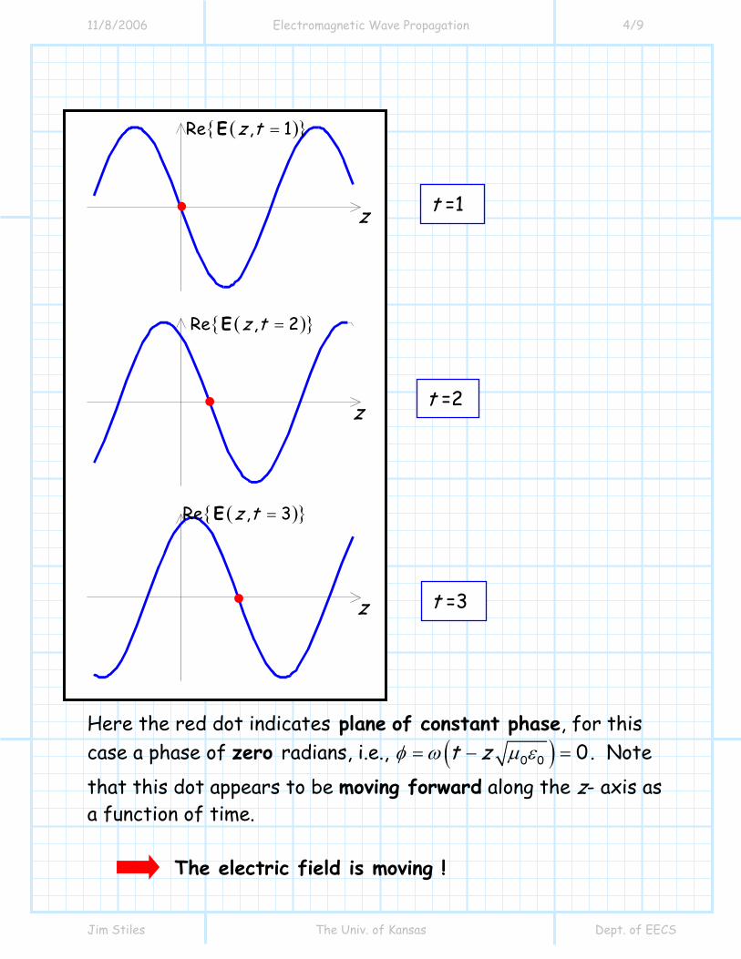
For this solution, the electric field is varying with time in a sinusoidal manner (that eigen function thing!), with an angular frequency of radians/secω . Note this field is a function of spatial coordinate z only, but the direction of the electric field is orthogonal to the z-axis. Q: What does this equation tell us about ( )r ,tE ? What is this electric field doing?? A: Lets plot ( ){ }Re r ,tE as a function of position z, for different times t, and find out!



Here the red dot indicates plane of constant phase, for this case a phase of zero radians, i.e., ( )0 0 0t zφ ω µ ε= − = . Note

that this dot appears to be moving forward along the z- axis as a function of time.

The electric field is moving !

( ){ }Re , 1z t =E

z

z

z t =1

t =2

t =3

( ){ }Re , 2z t =E

( ){ }Re , 3z t =E



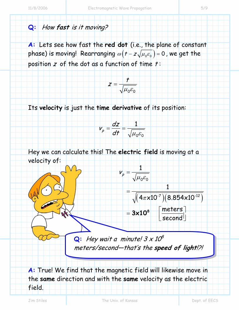
Q: How fast is it moving? A: Lets see how fast the red dot (i.e., the plane of constant phase) is moving! Rearranging ( )0 0 0t zω µ ε− = , we get the position z of the dot as a function of time t :

0 0

tzµ ε

=

Its velocity is just the time derivative of its position:

0 0

1p

dzvdt µ ε

= =

Hey we can calculate this! The electric field is moving at a velocity of:

( ) ( )

0 0

-7 -12

1

14 x10 8 854x10

meters second

pv

.

µ ε

π

=

=

⎡ ⎤= ⎢ ⎥⎣ ⎦83x10

A: True! We find that the magnetic field will likewise move in the same direction and with the same velocity as the electric field.

Q: Hey wait a minute! 3 x 108 meters/second—that’s the speed of light!?!



We call the combination of the two fields a propagating (i.e., moving) electromagnetic wave.

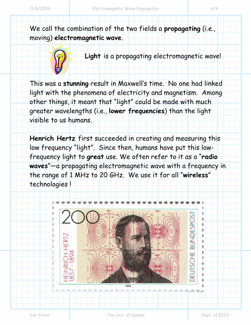
Light is a propagating electromagnetic wave! This was a stunning result in Maxwell’s time. No one had linked light with the phenomena of electricity and magnetism. Among other things, it meant that “light” could be made with much greater wavelengths (i.e., lower frequencies) than the light visible to us humans. Henrich Hertz first succeeded in creating and measuring this low frequency “light”. Since then, humans have put this low-frequency light to great use. We often refer to it as a “radio waves”—a propagating electromagnetic wave with a frequency in the range of 1 MHz to 20 GHz. We use it for all “wireless” technologies !



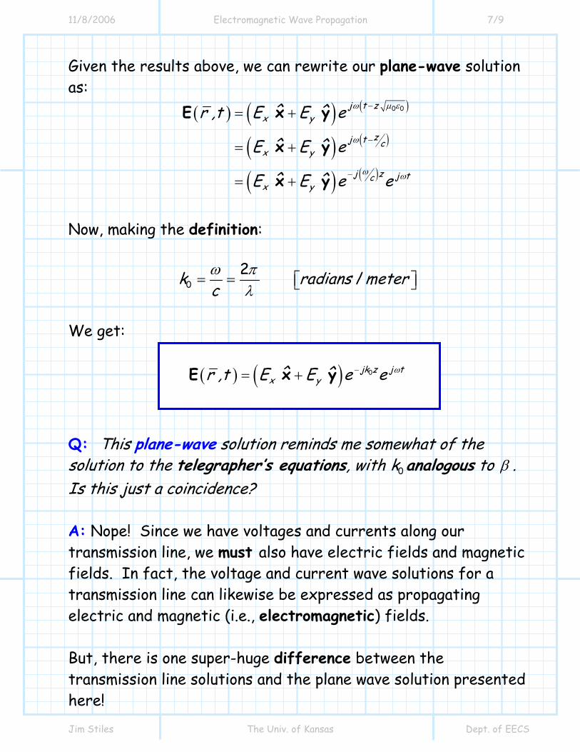
Given the results above, we can rewrite our plane-wave solution as:

( ) ( ) ( )

( ) ( )

( ) ( )

0 0j t zx y

zj t cx y

j z j tcx y

ˆ ˆr ,t E E e

ˆ ˆE E e

ˆ ˆE E e e

ω µ ε

ω

ω ω

−

−

−

= +

= +

= +

E x y

x y

x y

Now, making the definition:

02 /k radians meter

cω π

λ= = ⎡ ⎤⎣ ⎦

We get:

( ) ( ) 0jk z j tx yˆ ˆr ,t E E e e ω−= +E x y

Q: This plane-wave solution reminds me somewhat of the solution to the telegrapher’s equations, with 0k analogous to β . Is this just a coincidence? A: Nope! Since we have voltages and currents along our transmission line, we must also have electric fields and magnetic fields. In fact, the voltage and current wave solutions for a transmission line can likewise be expressed as propagating electric and magnetic (i.e., electromagnetic) fields. But, there is one super-huge difference between the transmission line solutions and the plane wave solution presented here!



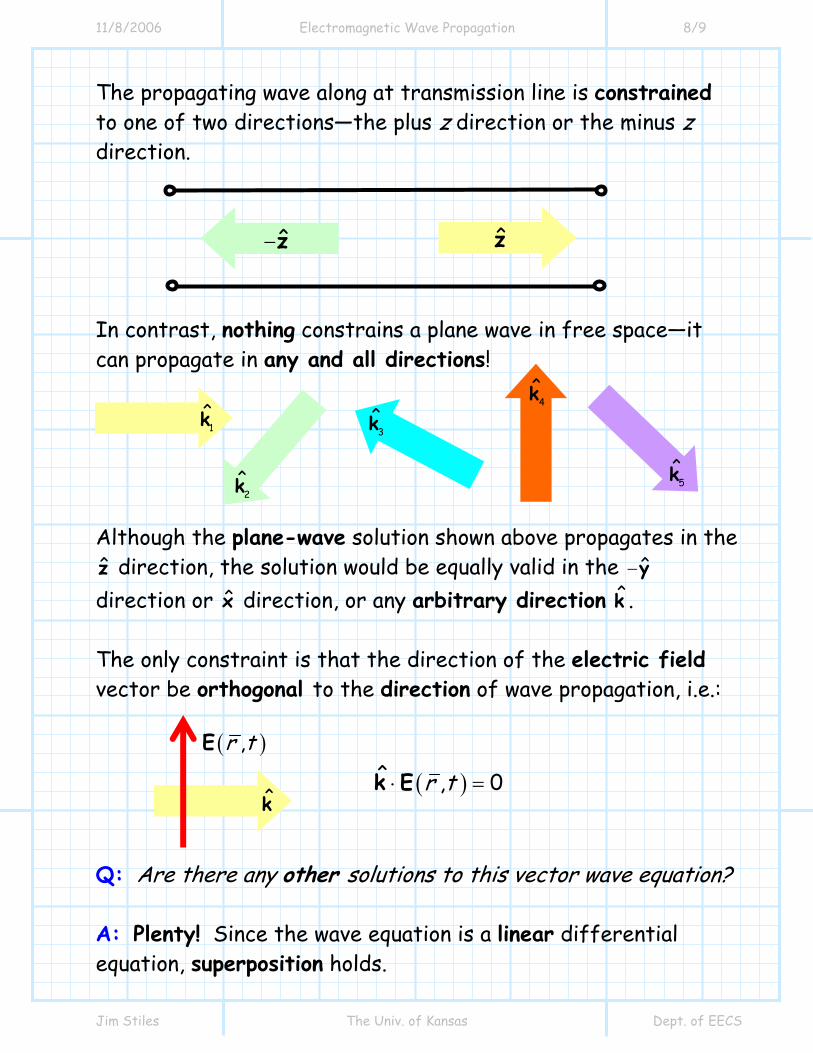
The propagating wave along at transmission line is constrained to one of two directions—the plus z direction or the minus z direction. In contrast, nothing constrains a plane wave in free space—it can propagate in any and all directions! Although the plane-wave solution shown above propagates in the z direction, the solution would be equally valid in the ˆ−y direction or x direction, or any arbitrary direction k . The only constraint is that the direction of the electric field vector be orthogonal to the direction of wave propagation, i.e.:

( )ˆ , 0r t⋅ =k E Q: Are there any other solutions to this vector wave equation? A: Plenty! Since the wave equation is a linear differential equation, superposition holds.

z ˆ−z

1k

2k

3k 4k

5k

k

( ),r tE



In other words, a weighted sum of solutions is also a solution. This means that we can (and often do) have multiple waves propagating simultaneously in all different directions. Moreover, there are many other solutions besides the plane-wave solution. The most relevant of these, perhaps, is the spherical wave:

( ) ( ) ( )( ) 0jk rj teˆ ˆr ,t E , E , e

rω

θ φθ φ θ φ−

= +E θ φ

Note the spherical wave is (most easily) expressed using the spherical coordinate system (i.e., coordinates , ,r θ φ and base vectors ˆˆ ˆ, ,r θ φ ). The spherical wave propagates outward from the origin (i.e., in the direction ˆ ˆ=k r ). In other words, a sphere of constant phase (as opposed to a plane of constant phase) propagates outward from the origin. Thus, this sphere of constant phase “expands” as a function of time—sort of like a balloon being filled with air! We likewise see from the expression above that the direction of the electric field is likewise orthogonal to the direction of wave propagation.

( ) ( )ˆ ˆ, , 0r t r t⋅ = ⋅ =k E r E

11/8/2006 The Poynting Vector 1/8


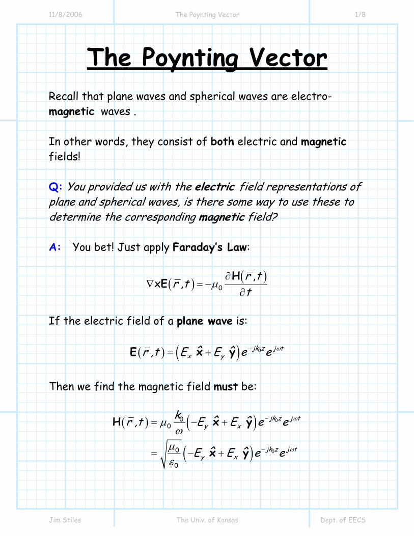
The Poynting Vector Recall that plane waves and spherical waves are electro-magnetic waves . In other words, they consist of both electric and magnetic fields! Q: You provided us with the electric field representations of plane and spherical waves, is there some way to use these to determine the corresponding magnetic field? A: You bet! Just apply Faraday’s Law:

( ) ( )0

,x ,

r tr tt

µ∂

∇ = −∂

HE

If the electric field of a plane wave is:

( ) ( ) 0jk z j tx yˆ ˆr ,t E E e e ω−= +E x y

Then we find the magnetic field must be:

( ) ( )

( )

0

0

00

0

0

jk z j ty x

jk z j ty x

k ˆ ˆr ,t E E e e

ˆ ˆE E e e

ω

ω

µω

µε

−

−

= − +

= − +

H x y

x y



Now, making the definition:

00

0

377 Ohmsµηε

= =

We find the corresponding magnetic field for our plane wave solution is thus:

( ) ( ) 00

jk z j ty xˆ ˆr ,t E E e e ωη −= − +H x y

The value 0η is know as the wave impedance, or sometimes called the characteristic impedance of free space.

Q: Why is 0η referred to as an impedance? Does it really have units of Ohms? A: Consider the magnitude of both ( )r ,tE and ( )r ,tH :

( ) ( ) ( )

( ) ( )( ) ( ) (

)

0 0

0 0

2

22

jk z j t jk z j tx y x y

j k z k z j t tx x y x

x y y y

x y

r ,t r ,t r ,tˆ ˆˆ ê e E E E E e e

ˆ ˆ ˆê e E E E E

ˆ ˆ ˆ Ê E E E

E E

ω ω

ω ω

∗

− + −∗ ∗

− − − ∗ ∗

∗ ∗

= ⋅

= + ⋅ +

= ⋅ + ⋅

+ ⋅ + ⋅

= +

E E E

x y x y

x x y x

x y y y

Therefore:

( )22

x yVr ,t E E m= +E



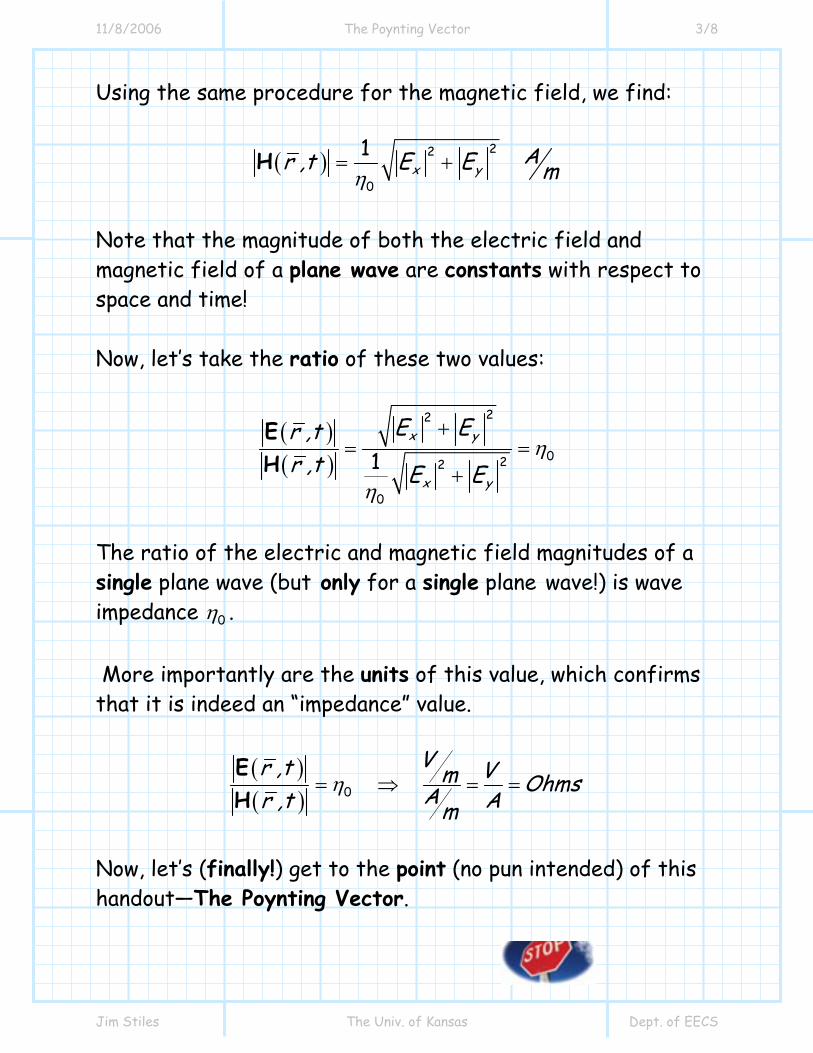
Using the same procedure for the magnetic field, we find:

( )22

0

1x y

Ar ,t E E mη= +H

Note that the magnitude of both the electric field and magnetic field of a plane wave are constants with respect to space and time! Now, let’s take the ratio of these two values:

( )( )

22

022

0

1x y

x y

E Er ,tr ,t E E

η

η

+= =

+

EH

The ratio of the electric and magnetic field magnitudes of a single plane wave (but only for a single plane wave!) is wave impedance 0η . More importantly are the units of this value, which confirms that it is indeed an “impedance” value.

( )( ) 0

Vr ,t Vm OhmsAr ,t Amη= ⇒ = =

EH

Now, let’s (finally!) get to the point (no pun intended) of this handout—The Poynting Vector.

jstiles

stop



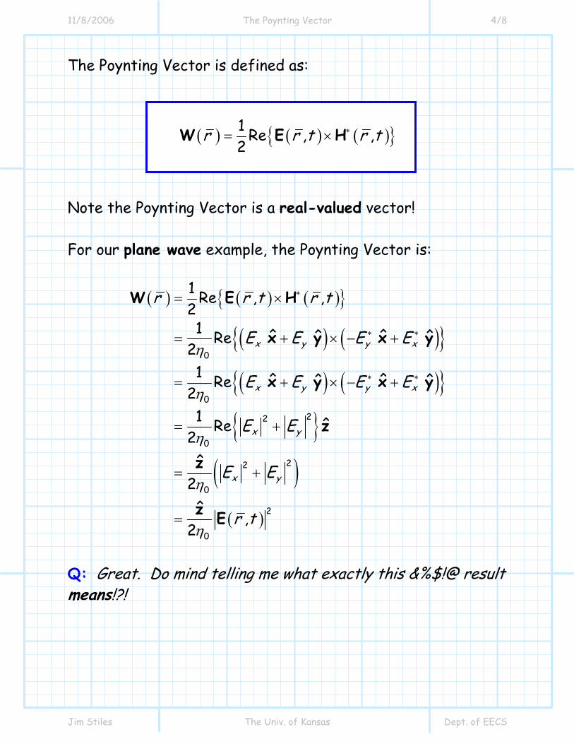
The Poynting Vector is defined as:

( ) ( ) ( ){ }1 Re , ,2

r r t r t∗= ×W E H

Note the Poynting Vector is a real-valued vector!

For our plane wave example, the Poynting Vector is:

( ) ( ) ( ){ }

( ) ( ){ }

( ) ( ){ }

{ }( )( )

0

0

22

0

22

0

2

0

1 Re , ,21 ˆ ˆˆ ˆRe

21 ˆ ˆˆ ˆRe

21 ˆRe

2ˆ

2ˆ

,2

x y y x

x y y x

x y

x y

r r t r t

E E E E

E E E E

E E

E E

r t

η

η

η

η

η

∗

∗ ∗

∗ ∗

= ×

= + × − +

= + × − +

= +

= +

=

W E H

x y x y

x y x y

z

z

z E

Q: Great. Do mind telling me what exactly this &%$!@ result means!?!



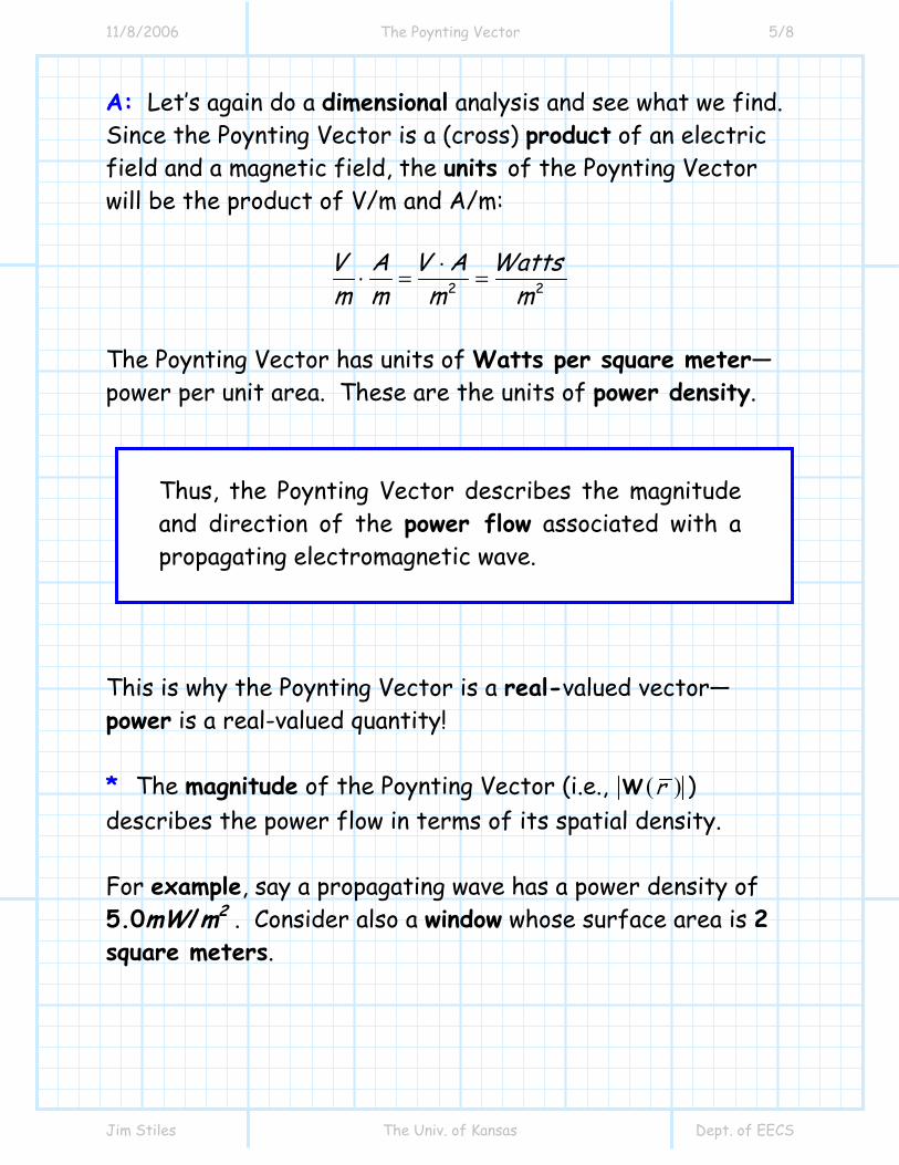
A: Let’s again do a dimensional analysis and see what we find. Since the Poynting Vector is a (cross) product of an electric field and a magnetic field, the units of the Poynting Vector will be the product of V/m and A/m:

2 2V A V A Wattsm m m m

⋅⋅ = =

The Poynting Vector has units of Watts per square meter—power per unit area. These are the units of power density.

Thus, the Poynting Vector describes the magnitude and direction of the power flow associated with a propagating electromagnetic wave.

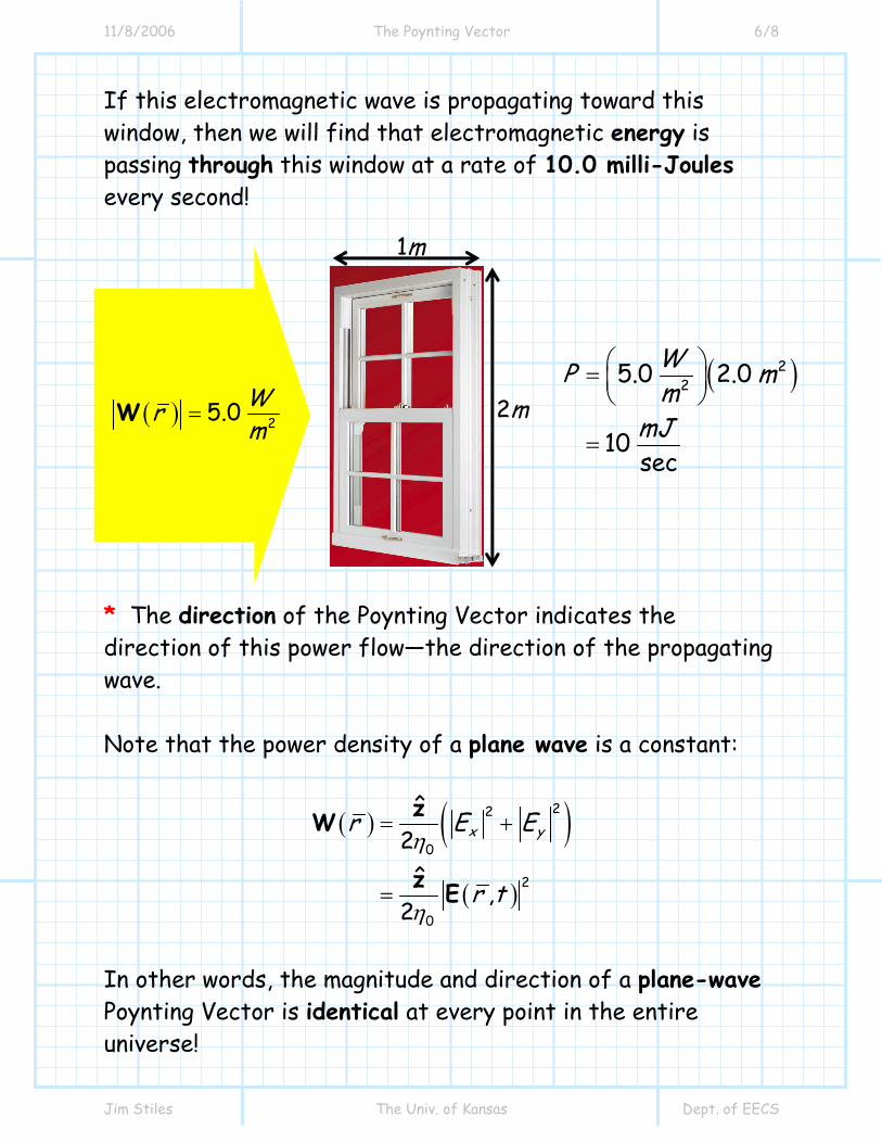
This is why the Poynting Vector is a real-valued vector—power is a real-valued quantity! * The magnitude of the Poynting Vector (i.e., ( )rW ) describes the power flow in terms of its spatial density. For example, say a propagating wave has a power density of 5.0mW/m2 . Consider also a window whose surface area is 2 square meters.



If this electromagnetic wave is propagating toward this window, then we will find that electromagnetic energy is passing through this window at a rate of 10.0 milli-Joules every second!

* The direction of the Poynting Vector indicates the direction of this power flow—the direction of the propagating wave. Note that the power density of a plane wave is a constant:

( ) ( )( )

22

0

2

0

ˆ2ˆ

,2

x yr E E

r t

= +

=

zW

z E

η

η

In other words, the magnitude and direction of a plane-wave Poynting Vector is identical at every point in the entire universe!

( )225.0 2.0

10sec

WP mm

mJ

⎛ ⎞= ⎜ ⎟⎝ ⎠

=( ) 25.0 Wr

m=W 2m

1m



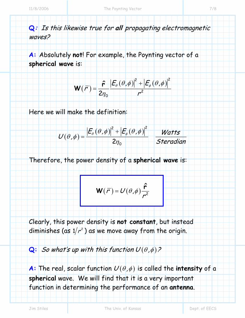
Q: Is this likewise true for all propagating electromagnetic waves? A: Absolutely not! For example, the Poynting vector of a spherical wave is:

( )( ) ( )

22

20

, ,ˆ2

E Er

r+

=rW θ φθ φ θ φη

Here we will make the definition:

( )( ) ( )

22

02E , E , WattsU ,

Steradian+

= θ φθ φ θ φθ φ

η

Therefore, the power density of a spherical wave is:

( ) ( ) 2

ˆ,r U

r=

rW θ φ

Clearly, this power density is not constant, but instead diminishes (as 21 r ) as we move away from the origin. Q: So what’s up with this function ( )U ,θ φ ? A: The real, scalar function ( )U ,θ φ is called the intensity of a spherical wave. We will find that it is a very important function in determining the performance of an antenna.



Q: Antenna? What does all this have to do with antennas? A: A radiating antenna in fact launches a spherical wave. The expression above thus describes the power density produced by a radiating antenna (when located at the origin).

iii antenna fundamentals - ku ittcjstiles/622/handouts/wave_propagation_package.pdf · 4/26/2005...

Documents