imaging of rod-airfoil aeroacoustics using a … · imaging of rod-airfoil aeroacoustics using a...

BeBeC-2012-20

IMAGING OF ROD-AIRFOIL AEROACOUSTICS USING ALOW-COST ACOUSTIC CAMERA

M. Debrouwere, L. Uyttersprot, J. Verwilligen, S. Probsting,D. G. Simons and F. Scarano

Faculty of Aerospace EngineeringDelf University of TechnologyKluyverweg 1, 2629 HS Delft

ABSTRACT

Along with stricter noise regulations in aviation comes the requirement to identify andeliminate sources of noise in aerodynamic designs. For this purpose, a phased array anddata acquisition system (acoustic camera) was designed and built by students of the Fac-ulty of Aerospace Engineering of Delft University of Technology. The performance ofthe phased array and different beamforming algorithms is evaluated with a variety of testcases, representative for the experiments conducted in moderate size wind tunnels (mod-els of 10cm to 30cm, working distance of 1m to 2m) as typically available in universitylaboratories. The considered test cases are rod-airfoil combinations, which produce low-frequency tonal noise. The scaled models are tested in an open jet non-anechoic verticalwind tunnel at flow speeds ranging from 15ms−1 to 40ms−1. The experiments presentseveral challenges, namely the low level of the emitted noise, the required high spatial res-olution and the refraction of sound waves travelling through the shear layer. The studydiscusses the specific developments and optimization of the low-cost acoustic camera foruse in the non-anechoic open jet wind tunnel of moderate size.

1 Introduction

Along with stricter noise regulations in aviation comes the requirement to identify andeliminate noise in aerodynamic designs. For this purpose an acoustic array can be used as adiagnostic tool which maps the noise sources. Over the past ten years extensive research hasbeen done to improve the functioning of those acoustic arrays [1], [4]. However, most acousticcameras remain very expensive. As an answer to this matter a group students of the Facultyof Aerospace Engineering of the Delft University of Technology designed and built a phasedarray and data acquisition system at the fraction of the cost of current commercially available

1

4th Berlin Beamforming Conference 2012 Debrouwere et al.

technology.

Originally this acoustic array was designed with as main purpose the noise source identi-fication of fly-overs of mid-range to long-range passenger aircraft. However, this paper aimsto analyse the performance of the phased array when used for a different application, namelythe application of the phased array for noise source identification in wind tunnel experiments.For this purpose a variety of test cases, representative for experiments conducted in moderatesize wind tunnels (models of 10cm to 30cm, working distance 1m to 2m) as typicallyavailable in university laboratories, were performed. The considered test cases are rod-airfoilcombinations, which produce low frequency tonal noise. The scaled models are tested in anopen jet non-anechoic vertical wind tunnel at flow speeds ranging from 15ms−1 to 40ms−1.The wind tunnel environment differs from the original fly-over environment in a number ofways which present several challenges for the noise source mapping. Among those challengesare the low level of the emitted noise, the required high spatial resolution and the refraction ofsound waves travelling through the shear layer. This study discusses the specific developmentsand optimization of the low-cost acoustic camera for use in the non-anechoic open jet windtunnel of moderate size.

The second section will discuss the experimental set-up and procedures that were used toanalyse the performance of the phased array. It will first give more details about the test caseitself, namely the rod-airfoil combinations. Consequently a more detailed description of theused acoustic camera together with the implemented adaptations specific for the wind tunneltest case will be given. The third section will provide the results together with a discussion.

2 Experimental set-up and procedures

2.1 Description of test cases

The performance of the acoustic camera is evaluated with a variety of measurements performedin an open-jet non-anechoic vertical wind tunnel of the Delft University of Technology at flowspeeds ranging from 15ms−1 to 40ms−1. This wind tunnel has a circular cross-section of60cm. The phased array was placed at a distance of 96.5cm from the centre line of the windtunnel as visible in Fig. 1(a). It is important to note that the centre point of the phased arraywas placed 7cm to the left of the centre line of the wind tunnel. All test cases consist of arod-airfoil combination, where the generic airfoil, which has a symmetric profile with a trailingedge thickness of 3mm, is placed parallel to the phased array. Three different cases were used:one rod parallel to the airfoil (Fig. 1(a)), one rod perpendicular to the airfoil (Fig. 1(b)) andtwo rods perpendicular to the airfoil (Fig. 1(c)). Here, the rods are always placed at a distanceof 18.5cm in front of the leading edge of the airfoil.

The rod-airfoil configuration in general is used as a benchmark test case for aeroacousticassessments of vortex-structure interaction broadband noise [2] [3]. In this case the airfoil isembedded in the wake of the upstream rod. This can represent features of a high-lift deviceconfiguration or a landing gear. In the rod-airfoil test set-up one main source of noise emissionis the vorticity shed by the rod convecting over the airfoil. Furthermore the blunt trailing edge

2


(a) Parallel rod, side view (b) Perpendicular rod, sideview

(c) Two perpendicular rods,front view

Figure 1: Schematic overview of the test set-up (not drawn up to scale)

of the airfoil and the associated vortex shedding also causes noise emission.

2.2 Acoustic camera for wind tunnel measurements

In order to identify noise sources in aerodynamic test cases a phased array and data acquisitionsystem (acoustic camera), designed and built by a group of students of the Faculty of AerospaceEngineering of Delft University of Technology, was used. The acoustic camera consists of 32microphone channels, placed on a flat plate of 2.38m by 1.60m in a spiral configuration. Forall measurements the sampling frequency was set at 50kHz. Furthermore the sampling time perblock was 0.2s, which corresponds to a frequency resolution of 5Hz. Furthermore the samplingtime per block was set to 0.2s. For every block of 0.2s a data transfer of 0.4s is needed.This results in a total measurement time of 0.6s times the number of blocks. The acousticcamera supports different beamforming algorithms. However, for clarity, only the conventionalbeamforming algorithm will be used in this paper. For a more detailed description of theacoustic camera the reader is referred to [8]. The next sections will describe modifications ofthe original beamforming software to tailor the acoustic camera to wind tunnel measurements.

Wind-correction

The key ingredient in almost any beamforming algorithm is the steering vector [5] , shown in Eq.1. It is a function of the frequency f , the distance from a microphone to the scan point ||xm−xs||and the travel time ∆t, the time required for the sound to arrive at the microphone. When nowind is present, this travel time is a linear function of the distance to the scan point, since soundwaves travel with the speed of sound. When a constant wind is present, this calculation is morecomprehensive. For our particular experiment it was assumed that the wind exiting the tunnelhas a uniform velocity while the air is stagnant outside this jet. The average flow velocity is

3


then used to compute the steering vector [5] given by

g =−e−2πi f ∆t(xm,xs)

4π||xm−xs||(1)

If a point source at location xs is considered under zero wind conditions, the sound willmove outward in a spherical fashion. If now a constant airspeed is introduced, each consecutivesphere will have moved with respect to the previous one with the speed of the flow. Thereforethe source appears to be at a different place at each instant in time. The problem is now to findthe time ∆t at which the sound wave has reached the observer.

In Fig. 2 the problem as described above is depicted. Here V ∆t is the distance the ‘virtual’source has moved when the sound arrives at the observer and xv is the distance to the virtualsource at that time. The angle α can be computed using the definition of the dot product (Eq.2), elaborated in Eq. 3.

Figure 2: The situation after time ∆t

xs ·V∆t = ||xs|| ||V∆t||cosα (2)

α = arccos(

xs ·V∆t||xs|| ||V∆t||

)(3)

With α known and observing that xv is equal to the speed of sound c times the travel time, thelaw of cosines can be formulated (Eq. 4). This is a quadratic equation, so the quadratic formulacan be used to determine ∆t (Eq. 5).

4


x2v = (c∆t)2 = x2

s +(V ∆t)2− xsV ∆t cosα (4)

∆t =xsV ∆t cosα±

√(−xsV ∆t cosα)2−4(V 2− c2)x2

s

2(V 2− c2)(5)

The results with this corrected steering vector are satisfying. The effect can be seen in Fig. 3and 4. The source is expected close to the white line of the rod. If no wind correction is appliedon the steering vector the source is detected further downstream of the rod (Fig. 3). When thecorrected steering vector is used the position of the source appears to be more accurate (Fig.4). In this case the rod was parallel to the airfoil’s leading edge and has a diameter of 4 mm.The wind speed is 30 m/s and the selected frequency range is 1550 to 1620 Hz, covering theexpected shedding frequency based on Strouhal’s relation.

Rod

LE

TE

x position [m]

y po

sitio

n [m

]

Sourceplot without Wind Correction

−0.2 −0.15 −0.1 −0.05 0 0.05 0.1 0.15 0.2

−0.5

−0.4

−0.3

−0.2

−0.1

0

0.1

1

2

3

4

5

6

7

x 104

Figure 3: Without wind correction

Rod

LE

TE

x position [m]

y po

sitio

n [m

]

Sourceplot with Wind Correction

−0.2 −0.15 −0.1 −0.05 0 0.05 0.1 0.15 0.2

−0.5

−0.4

−0.3

−0.2

−0.1

0

0.1

2

4

6

8

10

12

14

16

x 106

Figure 4: With wind correction

Averaging

In order to improve the results, multiple measurements were combined to filter out noise fromthe environment. The data acquisition system runs for several seconds during which multiplemeasurements are recorded. The system samples the microphone signals at a frequency of50000 Hz over a period of 0.2 s. Afterwards the system needs 0.4 s to package the data andsend it to the host computer. These two steps are repeated over the whole measurement time.This means that at the end of a measurement, a number of data-blocks are obtained. Since theexperiment is considered to be a statistically stationary process, all the blocks can be averagedto reduce noise [5]. A measurement contains approximately 25 blocks and the result of theaveraging is clearly visible in the spectral analysis of the microphone signals.

5


Horizontal scaling

For most of the test cases in these experiments, the sound sources are expected uniformly overthe whole span of the airfoil edges, or the rod. However due to irregularities, like a circularcross-section of the wind tunnel, this is not always shown by a source plot. The beamformingalgorithm tends to only detect and show the most intense spot in the field of view. In order tocorrect for this effect all the pixel lines perpendicular to the span of the airfoil can be scaled sep-arately. This will make sure that along the span, all sources are equally powerful, so a uniformspanwise source distribution is obtained. This method is inspired by techniques described in [6]and [7]. This however makes the scale on the source plot obsolete. This horizontal scaling isonly useful for sound source identification, not for determining the exact intensity. The effectof this process is illustrated by Fig. 5 and 6. Both figures are produced from the same dataset.In this case the rod is parallel to the airfoil’s leading edge and had a diameter of 4 mm. Thewind speed is 30 m/s and the frequency range is 1550 to 1620 Hz.

Rod

LE

TE

x position [m]

y po

sitio

n [m

]

Sourceplot without Horizontal Equalizing

−0.2 −0.15 −0.1 −0.05 0 0.05 0.1 0.15 0.2

−0.5

−0.4

−0.3

−0.2

−0.1

0

0.1

2

4

6

8

10

12

14

16

x 106

Figure 5: Without horizontal scaling

Rod

LE

TE

x position [m]

y po

sitio

n [m

]

Sourceplot with Horizontal Equalizing

−0.2 −0.15 −0.1 −0.05 0 0.05 0.1 0.15 0.2

−0.5

−0.4

−0.3

−0.2

−0.1

0

0.1

0

10

20

30

40

50

60

70

80

90

Figure 6: With horizontal scaling

3 Results and discussion

In this section the results of the measurement campaign will be presented and discussed. Theresults are divided among the three test cases described in section 2. Below each figure therepresented test case will be given with there corresponding letter as depicted in Fig. 1. Fur-thermore the freestream velocity V∞, the rod diameter dr and the frequency range f will begiven below each figure. The colour scales used in the figures show the relative normalisedpower emitted at the shown source locations, as perceived at the receiver’s location. In all thepresented cases the wind corrected steering vector described in section 2.2 was used. In almostall cases the loudest source in the test was the rod placed in the flow. The focus of this paperis how the shed vorticity reacts on the airfoil. Therefore the source plots created use frequencyranges outside the frequency range produced by the rod (given by the Strouhal relation). Thefrequency ranges of interest are determined based on the spectral analysis of a data set. Thelowest wind speed used in the experiment sequence is 25ms−1, since at lower wind speeds the

6


frequency of the shed vorticity becomes too low to result in useful resolutions. In each pictureevery pixel represents 2 x 2mm of the scanned region, this determines the finest difference thatcan be mapped in a source plot. This is not a limitation, but was chosen for convenience. Thispixel size results in reasonable computing time and is sufficient for these experiments. In total48 measurements were recorded, however to avoid repetition only the most interesting resultswill be shown and discussed.

3.1 One rod rarallel

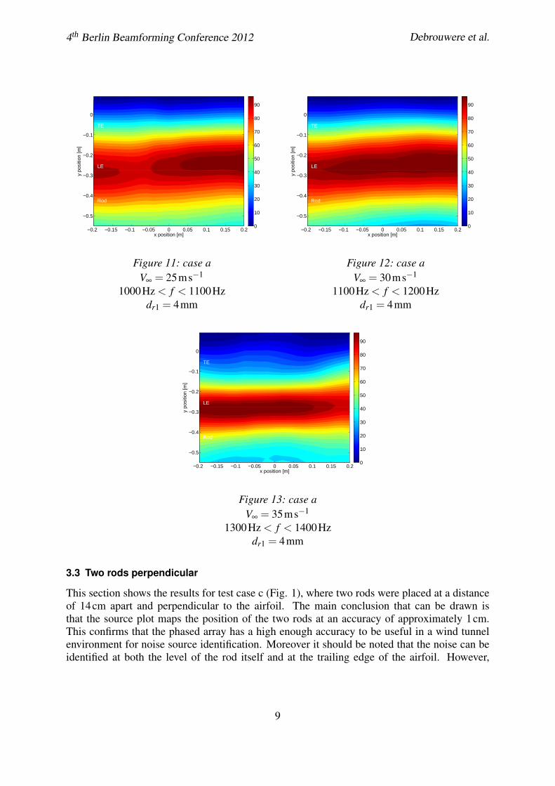
This section treats case (a) shown in Fig. 1, where one rod is placed upstream, parallel to theairfoil. Since in this case noise is expected to be uniform along the span of the wing, horizontalscaling is applied in all figures in this section. From Fig. 7, 9, 11, 12 and 13 it is clear that forthis test case, the noise emitted at the leading edge can clearly be identified. This confirms theexpectation that the rod causes vortex shedding which causes noise when it impinges on theairfoil leading edge. The noise emitted from the leading edge is nearly continuous over theentire span of the airfoil. This confirms that the horizontal scaling as introduced in section 2.2,gives appropriate results. Furthermore the noise is located at a line which nearly coincides withthe leading edge of the airfoil, confirming that the wind scaling is done correctly. For the casewhere the rod with a 3mm cross-section is used, it is also possible to identify the noise emittedat the trailing edge, as illustrated in Fig. 8 and 10. In contrast, when the 4mm diameter rod wasused, the noise at the trailing edge of the airfoil was non-identifiable. This could be due to thefact that the frequency of the noise emitted by the rod coincides with the noise emitted at thetrailing edge.

When focussing on the frequencies of the source plots a number of relations can be derived.The first two follow directly from the Strouhal relation, namely that a higher velocity leads tohigher frequencies and that a thicker rod leads to lower frequencies. Next to this it can be notedthat the frequency of the sound detected at the leading edge is always lower than the predictedfrequency of vortex shedding by the rod, when using the Strouhal with a Strouhal number of0.21. For example in Fig. 7 the Strouhal relation predicts a frequency of 2100Hz, whereasthe frequency where the noise emitted at the leading edge is found ranges from 1500Hz to1400Hz. When only focussing on the test case with a rod diameter of 3mm, it can also benoted that the noise emitted at the trailing edge has a higher frequency than the noise emittedat the leading edge.

3.2 One rod perpendicular

This section treats case b in Fig. 1, where one rod is placed upstream, perpendicular to therod. Since for this test set-up it is not expected to have uniform noise sources across the span,horizontal scaling is not applied here. A first observation in Fig 14 to 18 is that the presence ofthe rod is most easily distinguished at the trailing edge of the airfoil and not on the leading edge.This might be due to the fact that the vorticity shed behind the perpendicular rod is restrictedto a finite part of the airfoil’s span. The resulting surface pressure perturbations are scatteredfrom the trailing edge. A second observation is that the highest noise emission is located at anx-position of approximately 7cm to the right of the centre of the phased array. This corresponds

7


Rod

LE

TE

x position [m]

y po

sitio

n [m

]

−0.2 −0.15 −0.1 −0.05 0 0.05 0.1 0.15

−0.5

−0.4

−0.3

−0.2

−0.1

0

0

10

20

30

40

50

60

70

80

90

Figure 7: case aV∞ = 30ms−1

1300Hz < f < 1400Hzdr1 = 3mm

Rod

LE

TE

x position [m]

y po

sitio

n [m

]

−0.2 −0.15 −0.1 −0.05 0 0.05 0.1 0.15

−0.5

−0.4

−0.3

−0.2

−0.1

0

0

10

20

30

40

50

60

70

80

90


1700Hz < f < 1800Hzdr1 = 3mm

Rod

LE

TE

x position [m]

y po

sitio

n [m

]

−0.2 −0.15 −0.1 −0.05 0 0.05 0.1 0.15 0.2

−0.5

−0.4

−0.3

−0.2

−0.1

0

0

10

20

30

40

50

60

70

80

90


1400Hz < f < 1500Hzdr1 = 3mm

Rod

LE

TE

x position [m]

y po

sitio

n [m

]

−0.2 −0.15 −0.1 −0.05 0 0.05 0.1 0.15 0.2

−0.5

−0.4

−0.3

−0.2

−0.1

0

0

10

20

30

40

50

60

70

80

90


1900Hz < f < 2000Hzdr1 = 3mm

to our test-up since the rod was placed in the middle of the wind tunnel and the centre of thephased array was positioned 7cm to the left of the centre line of the wind tunnel. Furthermoreit can be noted that for the case where the rod with a diameter of 3mm was used, the sourceplots are not as clear. This could be caused by the fact that also the trailing edge of the airfoilhas a thickness of 3mm. When comparing the frequency range of the trailing edge noise of theperpendicular rod case (Fig. 8) to the parallel rod case (Fig. 15) with the same parameters, it isclear that the perpendicular rod-airfoil test set-up leads to higher frequencies.

8


Rod

LE

TE

x position [m]

y po

sitio

n [m

]

−0.2 −0.15 −0.1 −0.05 0 0.05 0.1 0.15 0.2

−0.5

−0.4

−0.3

−0.2

−0.1

0

0

10

20

30

40

50

60

70

80

90


1000Hz < f < 1100Hzdr1 = 4mm

Rod

LE

TE

x position [m]

y po

sitio

n [m

]

−0.2 −0.15 −0.1 −0.05 0 0.05 0.1 0.15 0.2

−0.5

−0.4

−0.3

−0.2

−0.1

0

0

10

20

30

40

50

60

70

80

90


1100Hz < f < 1200Hzdr1 = 4mm

Rod

LE

TE

x position [m]

y po

sitio

n [m

]

−0.2 −0.15 −0.1 −0.05 0 0.05 0.1 0.15 0.2

−0.5

−0.4

−0.3

−0.2

−0.1

0

0

10

20

30

40

50

60

70

80

90


1300Hz < f < 1400Hzdr1 = 4mm

3.3 Two rods perpendicular

This section shows the results for test case c (Fig. 1), where two rods were placed at a distanceof 14cm apart and perpendicular to the airfoil. The main conclusion that can be drawn isthat the source plot maps the position of the two rods at an accuracy of approximately 1cm.This confirms that the phased array has a high enough accuracy to be useful in a wind tunnelenvironment for noise source identification. Moreover it should be noted that the noise can beidentified at both the level of the rod itself and at the trailing edge of the airfoil. However,

9


Rod

LE

TE

x position [m]

y po

sitio

n [m

]

−0.2 −0.15 −0.1 −0.05 0 0.05 0.1 0.15 0.2

−0.5

−0.4

−0.3

−0.2

−0.1

0

0

10

20

30

40

50

60

70

80

90

Figure 14: case bV∞ = 25ms−1

2450Hz < f < 2550Hzdr1 = 3mm

Rod

LE

TE

x position [m]

y po

sitio

n [m

]

−0.2 −0.15 −0.1 −0.05 0 0.05 0.1 0.15 0.2

−0.5

−0.4

−0.3

−0.2

−0.1

0

0

10

20

30

40

50

60

70

80

90


2550Hz < f < 2650Hzdr1 = 3mm

Rod

LE

TE

x position [m]

y po

sitio

n [m

]

−0.2 −0.15 −0.1 −0.05 0 0.05 0.1 0.15 0.2

−0.5

−0.4

−0.3

−0.2

−0.1

0

0

10

20

30

40

50

60

70

80

90


1700Hz < f < 1800Hzdr1 = 4mm

Rod

LE

TE

x position [m]

y po

sitio

n [m

]

−0.2 −0.15 −0.1 −0.05 0 0.05 0.1 0.15 0.2

−0.5

−0.4

−0.3

−0.2

−0.1

0

0

10

20

30

40

50

60

70

80

90


2050Hz < f < 2150Hzdr1 = 4mm

similar to case b, at the leading of the airfoil no noise emission is found. This would mean thatin the case of a rod placed upstream perpendicular to an airfoil the noise scattered at the trailingedge is of higher intensity than the noise cause by the shed vorticity impinging on the leadingedge.

10


Rod

LE

TE

x position [m]

y po

sitio

n [m

]

−0.2 −0.15 −0.1 −0.05 0 0.05 0.1 0.15 0.2

−0.5

−0.4

−0.3

−0.2

−0.1

0

0

10

20

30

40

50

60

70

80

90


2350Hz < f < 2450Hzdr1 = 4mm

Rod 1Rod 2

LE

TE

x position [m]

y po

sitio

n [m

]

−0.2 −0.15 −0.1 −0.05 0 0.05 0.1 0.15 0.2

−0.5

−0.4

−0.3

−0.2

−0.1

0

0

10

20

30

40

50

60

70

80

90

Figure 19: case cV∞ = 35ms−1

2850Hz < f < 2950Hzdr1 = 3mmdr2 = 4mm

Rod 1Rod 2

LE

TE

x position [m]

y po

sitio

n [m

]

−0.2 −0.15 −0.1 −0.05 0 0.05 0.1 0.15 0.2

−0.5

−0.4

−0.3

−0.2

−0.1

0

0

10

20

30

40

50

60

70

80

90

Figure 20: case cV∞ = 40ms−1

2600Hz < f < 2800Hzdr1 = 3mmdr2 = 4mm

4 Conclusion

The purpose of this research is to determine if the developed low cost acoustic camera is suitablefor wind tunnel measurements. To prepare the camera for wind tunnel measurements, threeadaptations are done to the beamforming algorithm:

• Wind-correction to obtain a higher precision

11


• Averaging to filter out noise from the environment

• Horizontal scaling to identify noise over the whole airfoil span width

With these corrections measurements are performed in an open-jet non-anechoic vertical windtunnel at flow speeds ranging from 15ms−1 to 40ms−1. The model used in the wind tunnel is ageneric symmetric airfoil in combination with one or two rods placed upstream the airfoil. Theresults in section 3 show that different noise emitters in the wind tunnel set-up can clearly beseparated which validates the implemented adaptations and the usefulness of this camera in awind tunnel environment.

References

[1] R. P. Dougherty. “Beamforming in Acoustic Testing.” In Aeroacoustic Measurements(edited by T. J. Mueller), chapter 2, pages 62–97. Springer-Verlag Berln Heidelberg NewYork, 2002. ISBN 3-540-41757-5.

[2] M. C. Jacob, J. Boudet, D. Casalino, and M. Michard. “A rod-airfoil experiment as abenchmark for broadband noise modeling.” Theoretical and Computational Fluid Dy-namics, 19(3), 171–196, 2005. URL http://www.springerlink.com/index/M1E9PXKD9ERT9PMC.pdf.

[3] V. Lorenzoni. “Aeroacoustic investigation of rod-airfoil noise based on time-resolvedpiv.” Master of science thesis, Delft University of Technology, Delft, Netherlands,2008. URL http://www.lr.tudelft.nl/fileadmin/Faculteit/LR/Organisatie/Afdelingen_en_Leerstoelen/Afdeling_AEWE/Aerodynamics/Contributor_Area/Secretary/M._Sc._theses/doc/081227_thesis_Valerio_Lorenzoni.pdf.

[4] S. Oerlemans and P. Sijtsma. “Acoustic array measurements of a 1:10.6 scaled airbus a340model.” AIAA Paper, (2004-2924), 2004. URL http://www.springerlink.com/index/M1E9PXKD9ERT9PMC.pdf.

[5] S. Oerlemans and P. Sijtsma. “Phased array beamforming applied to wind tunnel and fly-over tests.” Technical report, National Aerospace Laboratory, 2010.

[6] P. Sijtsma. “Acoustic array measurements of a 1:10.6 scaled airbus a340 model.” Technicalreport, National Aerospace Laboratory, 2004.

[7] P. Sijtsma. “Acoustic array measurements at nlr.”, 2010. Presentation.

[8] R. van der Goot, M. Boon, J. Hendriks, K. Scheper, G. Hermans, W. van der Wal, D. Ragni,and D. Simons. “A Low Cost, High Resolution Acoustic Camera with a Flexible Micro-phone Configuration.” Paper, Delft University of Technology, Delft, Netherlands, 2012.

12

http://www.springerlink.com/index/M1E9PXKD9ERT9PMC.pdf


http://www.lr.tudelft.nl/fileadmin/Faculteit/LR/Organisatie/Afdelingen_en_Leerstoelen/Afdeling_AEWE/Aerodynamics/Contributor_Area/Secretary/M._Sc._theses/doc/081227_thesis_Valerio_Lorenzoni.pdf






imaging of rod-airfoil aeroacoustics using a … · imaging of rod-airfoil aeroacoustics using a...

Documents