imm - dtu electronic theses and dissertationsetd.dtu.dk/thesis/154735/imm3229.pdf · af imm, dtu....
TRANSCRIPT

The Genetic Algorithm for solving the
Dial-a-Ride Problem
Kristin Berg Bergvinsdottir
Kgs. Lyngby
Thesis-2004-37
IMM

Trykt af IMM, DTU

Preface
This theses is submitted in partial ful�llment of the requirements of the degree: Mas-
ter of Science in Engineering. The project was prepared by Kristin Berg Bergvinsdottirduring the period October 2003 to May 2004 at the Operations Research section at thedepartment of Informatics and Mathematical Modelling (IMM), Technical University ofDenmark (DTU). The work was supervised by lector Jesper Larsen.
I would like to thank my supervisor for his assistance throughout the project. He assistedme on all the stages of the work and was always prepared to assist. He was also full ofgood ideas and inspiration.
I wold also like to thank René Munk Jørgensen, who acted as an assistant supervisor. Hehad a great inside knowledge about the dial-a-ride problem and helped me to get a muchbetter understanding of the practical side of the problem. He was very supporting andencouraging throughout the entire working period.
Special thanks go to my family for their support, especially during the last phases of theproject.
Kgs. Lyngby, May 2004,
Kristín Berg Bergvinsdóttirs001341
3

4
Abstract in English
In this project the genetic algorithm (GA) is used to solve the dial-a-ride problem (DARP).In a dial-a-ride system customers are to be picked up and delivered within given timewindows by a transportation vehicle. The aim is to minimize transportation cost andmaximize the customer service level while satisfying the constraints.
The approach used to solve the DARP is the classical cluster-�rst, route-second strategy.That is, the customers are assigned to vehicles using a genetic algorithm and then arouting heuristic algorithm developed by Baugh et al. [2] is used to make a route for eachvehicle. The solution method is implemented in JAVA and tested on several randomlygenerated test problems. The test problems are taken from Cordeau and Laporte [4].Several improvement strategies to the initial solution method are proposed and the resultsfrom the best strategy are compared to the results obtained by Cordeau and Laporte.
Keywords:
Dial-a-Ride problem, meta-heuristic, combinatorial optimization, evolutionary algorithms,genetic algorithm, cluster-�rst, route-second, space-time nearest neighbour heuristic.
Resumé på dansk
I dette projekt er den genetiske algoritme (GA) brugt for at løse Dial-a-Ride Problemet(DARP). I DARP skal kunder hentes og a�everes af et transportmiddel indenfor givnetidsvinduer. Formålet er at minimere transport omkosninger og maximere kundeservicesamtidigt med at holde begrænsningerne.
Metoden der er brugt til at løse DARP er den klassiske cluster-først, rute-næst strategi.I første omgang er den genetiske algoritme er brugt til at tildele kunder til transportmidlerne og dernæst anvendes en rute algoritme lavet af Baugh et al. [2] til at lave rutentil hvert transport middel. Løsningsmetoden er implementeret i JAVA og testet medmange tilfældigt lavet test problemer. Test problemerne er lavet af Cordeau and La-porte [4]. Nogle forbedringsstrategier bliver præsenteret til den første løsningsmetode ogresultaterne fra den bedste strategi bliver sammenlignet med resultaterne af Cordeau andLaporte.
Nøgleord:
Dial-a-Ride Problemet, meta-heuristik, combinatorial optimering, evolutionary algoritme,genetiske algoritme, cluster-først, rute-næst, areal-tid nærmeste nabo heuristik.

Contents
1 Introduction 9
1.1 Examples of a Dial-a-Ride transportation system . . . . . . . . . . . . . . 9
1.2 Purpose of the project . . . . . . . . . . . . . . . . . . . . . . . . . . . . . 12
1.3 Outline . . . . . . . . . . . . . . . . . . . . . . . . . . . . . . . . . . . . . . 12
1.4 Abbreviations . . . . . . . . . . . . . . . . . . . . . . . . . . . . . . . . . . 13
2 Dial-a-ride problem 15
2.1 Characteristics of the dial-a-ride problem . . . . . . . . . . . . . . . . . . 15
2.2 Customers with special needs . . . . . . . . . . . . . . . . . . . . . . . . . 16
2.3 Multi-objective optimization . . . . . . . . . . . . . . . . . . . . . . . . . . 16
2.4 Static vs. dynamic dial-a-ride problem . . . . . . . . . . . . . . . . . . . . 17
2.5 Inbound vs. outbound customers . . . . . . . . . . . . . . . . . . . . . . . 18
2.6 Problem formulation . . . . . . . . . . . . . . . . . . . . . . . . . . . . . . 18
2.7 Notation in the Mathematical Model . . . . . . . . . . . . . . . . . . . . . 21
2.8 Mathematical model . . . . . . . . . . . . . . . . . . . . . . . . . . . . . . 22
2.9 Objective function . . . . . . . . . . . . . . . . . . . . . . . . . . . . . . . 22
2.10 Constraints . . . . . . . . . . . . . . . . . . . . . . . . . . . . . . . . . . . 23
2.10.1 Depot constraints . . . . . . . . . . . . . . . . . . . . . . . . . . . . 23
2.10.2 Routing constraints . . . . . . . . . . . . . . . . . . . . . . . . . . . 23
2.10.3 Precedence constraints . . . . . . . . . . . . . . . . . . . . . . . . . 23
2.10.4 Timing constraints . . . . . . . . . . . . . . . . . . . . . . . . . . . 24
2.10.5 Capacity constraints . . . . . . . . . . . . . . . . . . . . . . . . . . 25
2.10.6 Linearization of constraints . . . . . . . . . . . . . . . . . . . . . . 26
2.11 Related problems . . . . . . . . . . . . . . . . . . . . . . . . . . . . . . . . 26
2.12 The Dial-a-ride problem is NP-hard . . . . . . . . . . . . . . . . . . . . . 28
5
6 CONTENTS
3 Previous Work 29
3.1 Jaw et al. . . . . . . . . . . . . . . . . . . . . . . . . . . . . . . . . . . . . 29
3.2 Baugh et al. . . . . . . . . . . . . . . . . . . . . . . . . . . . . . . . . . . . 30
3.3 Cordeau and Laporte . . . . . . . . . . . . . . . . . . . . . . . . . . . . . . 32
3.4 Jih et al. . . . . . . . . . . . . . . . . . . . . . . . . . . . . . . . . . . . . . 33
3.5 Pereira et. al . . . . . . . . . . . . . . . . . . . . . . . . . . . . . . . . . . 34
3.6 Comparison . . . . . . . . . . . . . . . . . . . . . . . . . . . . . . . . . . . 36
4 Solution method 39
4.1 Choosing the solution method . . . . . . . . . . . . . . . . . . . . . . . . . 39
4.2 The Genetic Algorithm . . . . . . . . . . . . . . . . . . . . . . . . . . . . . 41
4.2.1 Original version of GA . . . . . . . . . . . . . . . . . . . . . . . . . 43
4.2.2 Other versions of GA . . . . . . . . . . . . . . . . . . . . . . . . . . 43
4.2.3 Convergence . . . . . . . . . . . . . . . . . . . . . . . . . . . . . . . 44
4.2.4 Chromosome representation . . . . . . . . . . . . . . . . . . . . . . 45
4.2.5 Schemata . . . . . . . . . . . . . . . . . . . . . . . . . . . . . . . . 46
4.2.6 Population size . . . . . . . . . . . . . . . . . . . . . . . . . . . . . 47
4.2.7 Initial population . . . . . . . . . . . . . . . . . . . . . . . . . . . . 48
4.2.8 Stopping criteria . . . . . . . . . . . . . . . . . . . . . . . . . . . . 48
4.2.9 Fitness calculations . . . . . . . . . . . . . . . . . . . . . . . . . . . 48
4.2.10 Selection mechanism . . . . . . . . . . . . . . . . . . . . . . . . . . 49
4.2.11 Modifying operators . . . . . . . . . . . . . . . . . . . . . . . . . . 51
4.3 Modi�ed space-time nearest neighbour heuristic . . . . . . . . . . . . . . . 55
5 Implementation 57
5.1 Overview of the solution method . . . . . . . . . . . . . . . . . . . . . . . 57
5.2 Relaxation . . . . . . . . . . . . . . . . . . . . . . . . . . . . . . . . . . . . 58
5.2.1 E�ect of arrival time to destination . . . . . . . . . . . . . . . . . . 60
5.3 The initial heuristic - GA1 . . . . . . . . . . . . . . . . . . . . . . . . . . . 61
5.3.1 Clustering using GA . . . . . . . . . . . . . . . . . . . . . . . . . . 62
5.3.2 Routing strategy . . . . . . . . . . . . . . . . . . . . . . . . . . . . 67
5.3.3 Overview of GA1 . . . . . . . . . . . . . . . . . . . . . . . . . . . . 68
5.4 Improvements to GA1 . . . . . . . . . . . . . . . . . . . . . . . . . . . . . 69

CONTENTS 7
6 Experimental results 73
6.1 Data . . . . . . . . . . . . . . . . . . . . . . . . . . . . . . . . . . . . . . . 74
6.2 Testing and tuning the initial heuristic - GA1 . . . . . . . . . . . . . . . . 76
6.2.1 Selecting values for the parameters in the GA . . . . . . . . . . . . 76
6.3 Selecting values for the routing parameters in GA1 . . . . . . . . . . . . . 81
6.3.1 GA1 - Customers choice . . . . . . . . . . . . . . . . . . . . . . . . 82
6.3.2 GA1 - Operators choice . . . . . . . . . . . . . . . . . . . . . . . . 85
6.3.3 Weights chosen and convergence . . . . . . . . . . . . . . . . . . . . 86
6.4 Improving the initial heuristic . . . . . . . . . . . . . . . . . . . . . . . . . 87
6.4.1 Size of generation equals population size - GA2 . . . . . . . . . . . 88
6.4.2 Number of duplicates reduced - GA3 . . . . . . . . . . . . . . . . . 88
6.4.3 Reducing the randomness in the heuristic - GA4 . . . . . . . . . . . 89
6.4.4 Heuristic run twice and total number of iterations constant - GA5 . 92
6.5 The best improvement . . . . . . . . . . . . . . . . . . . . . . . . . . . . . 95
6.6 Comparison with Cordeau and Laporte results . . . . . . . . . . . . . . . . 95
6.7 Summary . . . . . . . . . . . . . . . . . . . . . . . . . . . . . . . . . . . . 97
7 Conclusion 99
Bibliography 101
A JAVA source code 103

8 CONTENTS
Chapter 1
Introduction
In the dial-a-ride problem (DARP) customers give a transportation operator requests fortransportation. A request consists of a speci�ed pickup (origin) location and drop o�(destination) location along with a desired departure or arrival time and the number ofpassengers to be transported. The problem is to determine the best routing schedule forthe transporting vehicles, which minimizes overall transportation cost and yet maintainsa high level of service to customers. The service level estimation is usually based on theride times of the customers and deviations from desired departure or arrival times. It isvery hard to combine these con�icting factors, small cost of transportation versus highservice level, so a good compromise is what is aimed at.
1.1 Examples of a Dial-a-Ride transportation system
The dial-a-ride transportation system is used to describe a variety of transportation ser-vice systems. The simplest form of a dial-a-ride transportation system is the taxi trans-portation system. In the taxi system, a customer calls in with his request and is thentransported directly from his pickup location to destination location. That is an exampleof a door-to-door transportation system. The aim of the dial-a-ride problem here, is tominimize the operators cost and maximize service to customers. The operators cost is de-creased by minimizing the number of taxis standing by, waiting to service customers andthe service level is increased by minimizing the waiting times of the customers before thetaxi's arrival, since if the customer has to wait too long, he will turn his business elsewhere.
Another example of a dial-a-ride system is the specialized transportation, that is thetransportation of for example children, disabled and elderly people. These specializedtransports are usually provided by local authorities. The customers also call in theirtransportation requests, but here larger vehicles, such as mini busses o� various capaci-ties, are used to transport the passengers. In this kind of transportation it is also necessaryto consider the di�erent needs of the customers. Some customers require just a regularseat, others have to be seated in their wheelchair, while again others may have to lie downwhen being transported.
9

10 Chapter 1. Introduction
Fixed Route Transportation Specialized Transportation TaxiLevel of service
Cos
t
Figure 1.1: The three di�erent modes of transportation cost more as the level of service increases. Inthis graph it is assumed that the cost increases linearly for �xed route, specialized and taxi
transportation.
In order to decrease transportation costs it is necessary to organize the transportation insuch a way, that di�erent customers and their companions share a ride. That is, a customermight not be transported directly from his pickup location to his destination location butinstead other customers could be dropped o� or picked up in between. Therefore the dial-a-ride problem becomes more complex than what was the case in the taxi transportationsystem. There it was necessary to minimize the number of vehicles used for transportationbut here it is also necessary to minimize the total distance and/or route duration for allthe vehicles used in the transport.
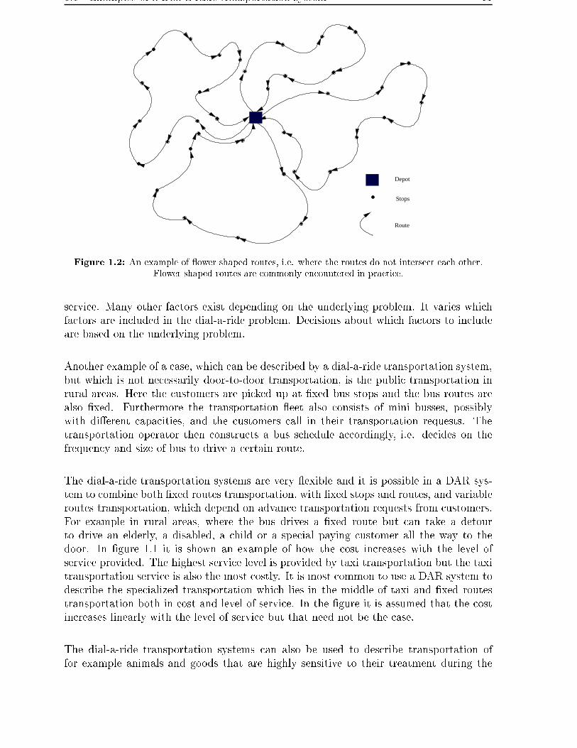
As in the taxi system it is also necessary to consider the customers service levels, eventhough the customers usually cannot freely choose their transportation operator service,since it is most often a publicly provided service. But lack of punctuality due to late arrivalby the transportation operator can cause problems and cost money in other organizations,which are perhaps also providing services to the customer. The unsatis�ed customer willdemand improvements and is sometimes entitled to that by rules or regulations or simplyby moral law. The estimation of customers service level in this case is mainly based ondeviations in arrival time and excess ride time, i.e. how much longer a customer has tosit in the bus than if it were a direct transport. Another factor to consider with regardsto the service level is the amount of time a customer has to sit in a halting vehicle. Thevehicle may have to halt in order to arrive at a correct time to collect or drop o� a cus-tomer. Waiting times like this are tedious for the customers and cause dissatisfaction.Yet another factor that can be considered when looking at the service level is the shapeof the route driven by the bus. That is, even though it might be optimal to drive in manyloops crossing them-selves it does not look like a good plan for the customer or even thebus driver. Such routes do therefore not seem practical. Instead the usual �ower shapedroutes where di�erent routes do not intersect, see �gure 1.2, are used, even though theyare more expensive. Other factors such as comfortability of vehicles, the manners of thebus driver and etc. are much harder to measure and will not be included in the dial-a-rideproblem. These are examples of the many di�erent factors that can in�uence the level of
1.1 Examples of a Dial a Ride transportation system 11
Stops
Route
Depot��������
��������
����
��������
���
���
��������
���
���
���
���
������
������
���
���
���
���
������
������
��������
��������
��������
����
������
������
���
���
����
��������
���
���
������
������
��������
����
����
������
������
����
����
����
��������
����
���
���
����
��������
���
���
������
������
Figure 1.2: An example of �ower shaped routes, i.e. where the routes do not intersect each other.Flower shaped routes are commonly encountered in practice.
service. Many other factors exist depending on the underlying problem. It varies whichfactors are included in the dial-a-ride problem. Decisions about which factors to includeare based on the underlying problem.
Another example of a case, which can be described by a dial-a-ride transportation system,but which is not necessarily door-to-door transportation, is the public transportation inrural areas. Here the customers are picked up at �xed bus stops and the bus routes arealso �xed. Furthermore the transportation �eet also consists of mini busses, possiblywith di�erent capacities, and the customers call in their transportation requests. Thetransportation operator then constructs a bus schedule accordingly, i.e. decides on thefrequency and size of bus to drive a certain route.
The dial-a-ride transportation systems are very �exible and it is possible in a DAR sys-tem to combine both �xed routes transportation, with �xed stops and routes, and variableroutes transportation, which depend on advance transportation requests from customers.For example in rural areas, where the bus drives a �xed route but can take a detourto drive an elderly, a disabled, a child or a special paying customer all the way to thedoor. In �gure 1.1 it is shown an example of how the cost increases with the level ofservice provided. The highest service level is provided by taxi transportation but the taxitransportation service is also the most costly. It is most common to use a DAR system todescribe the specialized transportation which lies in the middle of taxi and �xed routestransportation both in cost and level of service. In the �gure it is assumed that the costincreases linearly with the level of service but that need not be the case.
The dial-a-ride transportation systems can also be used to describe transportation offor example animals and goods that are highly sensitive to their treatment during the

12 Chapter 1. Introduction
transportation. The possibilities of usages are many and therefore it is very important toinvestigate the dial-a-ride problem in detail.
1.2 Purpose of the project
The work performed in this project is purely theoretical, i.e. the problem to be investi-gated is not based on a speci�c real-life problem. The problem will although be formulatedbased on realistic assumptions taken from a Danish transportation system.
The main goal of this project is to model and solve the dial-ride-problem using a solu-tion method, which has not yet been used to solve the dial-a-ride problem. The solutionmethod of choice in this project is cluster-�rst and route-second. The clustering willbe solved using the genetic algorithm and the routing will be determined by a modi�edspace-time nearest neighbour heuristic developed by Baugh et al. [2].
The solution method will be implemented in JAVA and tested using randomly createddata sets generated by Cordeau and Laporte [4]. The results obtained in this project arecompared with the results obtained by Cordeau and Laporte.
1.3 Outline
The remainder of this report will be divided into six chapters, which are described herebrie�y.
The dial-a-ride problem will be described in more detail in chapter 2, where an overviewwill be given of the most important related problems. A discussion of a multi-objectiveoptimization, followed by a discussion of the di�erence between the static and the dynamicdial-a-ride problem and also the di�erence between an outbound and inbound customer.There after the problem that is considered in this work is formulated and the mathematicalmodel for the DARP will be presented. There will be a description of the objectivefunction as well as the constraints. Lastly the NP-hardness of DARP will be addressedshortly.
In chapter 3 a short introduction to the history of the research on the dial-a-ride prob-lem is given. There will also be a description of some of the work that has previouslybeen published about the dial-a-ride problem and related problems. The work describedis work that has given inspiration and ideas to this project.
Chapter 4 gives a description of the solution method chosen to solve the DARP. Thesolution method is based on the cluster-�rst, route-second strategy. The clustering is theassignment of customers to vehicles, which is solved using the genetic algorithm. In therouting stage the customers already assigned to a vehicle are ordered, i.e. the actual route

1.4 Abbreviations 13
of the vehicle is constructed. The routing is solved using a heuristic adopted from Baughet al. [2]. The chapter starts by explaining the choice of the solution method followedby a description of the genetic algorithm and the modi�ed space time nearest neighbourheuristic.
In chapter 5 the implementation of the solution method chosen for solving the dial-a-rideproblem will be described. The problem is simpli�ed through relaxation of constraintsand solved in two stages, i.e. cluster-�rst, route-second. An initial heuristic is developedand several improvements proposed.
The experimental results are presented in chapter 6. The implemented algorithm willbe tested on several randomly generated problem instances constructed by Cordeau andLaporte [4]. The chapter will start by an introduction to the data instances used. Thenthe some parameters in the genetic algorithm are tuned and the in�uence of the weightson the di�erent parts of the objective function will be investigated. Next the initial al-gorithm will be tested on several instances. Thereafter some experiments to improve thealgorithm are tested. Lastly the best strategy found will be tested further and comparedwith the results found by Cordeau and Laporte.
The �nal conclusions of this project will be given in chapter 7.
1.4 Abbreviations
Table 1.1: Table of abbreviations.Abbreviation Full text
CPU Central Processing UnitDAR Dial-a-RideDARP Dial-a-Ride problemGA Genetic AlgorithmLP Linear ProblemMILP Mixed-Integer Linear ProblemMTC Montreal Transit CommissionNP-hard Non-deterministic Polynomial-time hardOR Operations ResearchPDP Pickup and Delivery ProblemTSP Travelling Salesman ProblemTW Time WindowsVRP Vehicle Routing ProblemVRPB Vehicle Routing Problem with Backhauls

14 Chapter 1. Introduction

Chapter 2
Dial-a-ride problem
In this chapter a more detailed description of the dial-a-ride problem is presented andrelated issues will be addressed. First the characteristics of the DARP are discussed andthe multi-objective optimization is described. An introduction of the static and dynamicversions of the DARP and the di�erence between an outbound and inbound passengerwill be given. Then a formulation of the speci�c problem used in the remainder of thisreport is given.
A basic mathematical model for the dial-a-ride problem with time windows is also pre-sented along with a discussion of the various constraints in the problem and the objectivefunction. The mathematical model that will be presented is very similar to the mathemat-ical model presented by Jørgensen [11] with auditorial extensions some of which are takenfrom Baugh et al. [2]. The chapter ends by a description of related problems followed bya discussion of the di�culty in solving the dial-a-ride problem since it can be proven tobe NP-hard1.
2.1 Characteristics of the dial-a-ride problem
The main characteristics of the static dial-a-ride problem with time windows will be de-scribed shortly in this section. These characteristics lay the foundation for formulatingthe mathematical model for the problem.
The objective of the dial-a-ride problem is to minimize total transportation costs and atthe same time maximize the level of service provided to the customers. In this project itis assumed that the maximization of the level of service is to be equivalent to minimizingthe unhappiness of the customers. The customers must be picked up or delivered withina given time interval. It is assumed that all customer requests are known in advance.It is required that each vehicle starts and ends in a depot but not necessarily the samedepot. The customers must �rst be picked up and then dropped o� by the same vehicle.
1In computational complexity theory, NP-hard refers to the class of decision problems that containsall problems H such that for all decision problems L in NP there is a polynomial-time many-one reductionto H
15

16 Chapter 2. Dial a ride problem
The vehicles have a �xed capacity, which may not be exceeded at any time. There is alsoan upper limit on the route duration for each vehicle and ride time for each customer.The constraints on time windows, ride times, route duration and capacity of the vehiclescan either be presented as soft or hard constraints. Hard constraints are constraints thatcannot be violated while soft constraints can be violated but it adds to the cost. Whichtype of constraint is used, hard or soft, is governed by the underlying problem.
2.2 Customers with special needs
Since the dial-a-ride systems are often used to describe cases which involve the transporta-tion of elderly and/or disabled persons this needs to be taken into account when makingthe model. The needs of these passengers are not the same as for other passengers. Theymay need assistance to get into/out of the vehicle, need special seats and so on. In or-der to get these factors into the model there is usually de�ned a service time associatedwith each stop, which accounts for the bus driver helping the passenger into the bus andsecure him on the bus. The need for special seats can be incorporated into the modelby specifying di�erent capacities for each seat type on the vehicle and then keeping trackof the load changes in each seat type. Another possibility is to de�ne the vehicles withone capacity and then de�ne the needs for special seats in number of regular seats. Forexample one passenger in a wheelchair needs two regular seats and a lying person needsfour regular seats on the bus.
2.3 Multi-objective optimization
In the dial-a-ride problem the objective is to minimize total transportation cost and min-imize the customer unhappiness. This kind of a optimization problem is a multi-objectiveoptimization problem. A multi-objective optimization problem involves a simultaneousoptimization of more than one objective function. The multi-objective function can bestated mathematically as follows:
Minimize v(h) =
v1(h)v2(h)...vσ(h)
(2.1)
where vi(h), i = 1, ..., σ are the σ objective functions in the multi-objective problem. It isunlikely that the di�erent objectives can be optimized by the same parameters. Thereforesome kind o� trade-o� between the criteria in the objective function is needed to ensurea satisfactory results. The concept of �optimality� does not apply directly for multi-objective optimization problems. A useful replacement is the notion of Pareto optimality.Essentially, a vector h∗ is said to be Pareto optimal for the multi-objective function 2.1 ifall other vectors h have a higher value for at least one of the objective functions (vi(·)).
The multi-objective problems are usually solved by combining the multiple objectives intoone scalar objective. The solution to the scalar objective is a Pareto optimal point for

2.4 Static vs. dynamic dial a ride problem 17
the original multi-objective function. A standard technique for combining the multipleobjectives in a multi-objective problem is to minimize a positively weighted sum of theobjectives, that is:
σ∑i=1
wivi(h), wi > 0, i = 1, 2, ..., σ (2.2)
The selection of the values of the weights wi is based on the importance of the di�erentobjectives and the importance of each objective evaluated by the user.
It is possible to handle the multi-objective function in other ways, e.g. by a multilevelprogramming. In the multilevel programming the objectives are ordered by importance.Next a set of points that optimizes the most important objective is found. Then thepoints in this set that optimize the second most important objective are found and soforth until all objectives have been optimized on successively smaller sets.
2.4 Static vs. dynamic dial-a-ride problem
Dial-a-ride transportation systems can be operated according to one of two modes, eitherstatic or dynamic.
In static mode all the transportation requests are known in advance. It is therefore pos-sible to plan the actual routes of the vehicles in advance. The static problem can also beused in the long-term decision, strategy, and planning process. In this case the informa-tion needed to create the static dial-a-ride problem, is constructed using historical dataor forecasted data. Di�erent scenarios are created and solved. In a way the solutions areused in a simulation process. The results are used as a reference giving a better overviewof the e�ects of potential events or trends and the e�ects of di�erent solution methods.
In dynamic mode the transportation requests are not known, or only partially known inadvance. The requests are instead gathered during the planning horizon when the cus-tomers call in with their transportation demands. In the dynamic case the actual routesof the vehicles are constructed in real-time. When solving the dynamic problem, thestatic problem is often solved �rst, based on requests known beforehand. That solutionis then used as a initial solution. This initial solution will then be modi�ed when a newtransportation request is received. This modi�cation can be performed by solving thestatic case over and over again. However it is usually not very e�cient so it will be betterto use a faster reopimization algorithm to resolve the problem each time a new request isreceived [11].
The solution methods used in the dynamic case must be very fast since the customer hasto be informed about whether his request can be met or not, and if so at what time heis to expect his ride, while he is still on the phone. In the static case however the timeused to solve the problem is not nearly as important, since requests are received the daybefore.

18 Chapter 2. Dial a ride problem
2.5 Inbound vs. outbound customers
The DARP customers can be divided into two groups, namely groups consisting of in-bound and outbound customers.
Inbound customers are customers that are located somewhere, perhaps at work, school orhospital, and need to be driven somewhere else, usually home. They need to be picked upafter work, school or hospital appointment at a speci�c point in time. It is also acceptableto collect them a little later than that time but not earlier since they are not ready toleave earlier. There is not a speci�c time window on their arrival time to their destinationlocation.
Outbound customers are customers that are to be picked up somewhere and then be de-livered somewhere else before a certain point in time. For example a person who needsto be driven from her home and to the doctors o�ce, where she needs to be at 3 o'clock.Here the customer can be picked up at any time but the delivery has to be no later than3 o'clock. Here no speci�c time windows are associated with the pickup location.
There is therefore either a time window constraint on the pickup or drop o� time for eachcustomer in the dial-a-ride system. Usually time windows for both acceptable pickup anddelivery times for each customer are de�ned. The time window, which is not speci�edby the customer, is derived from the allowed ride time of the customer speci�ed by thetransportation operator. A discussion of how the time windows can be set in DARP ispresented in section 2.10.4.
2.6 Problem formulation
There are a number of ways to formulate a dial-a-ride problem, which usually depend onthe underlying real-life problem. In this project there is no explicit real-life problem tosolve and the formulation of the problem can therefore be chosen freely. The problemformulation will however be focused on practical considerations as they are in the Danishtransportation sector, see Jørgensen [11].
The problem that will used in this report is formulated in the following way:
• The dial-a-ride transportation system
In this report focus will be set on a DAR transportation system that have customersto be transported from door to door but not necessarily directly. That is, customersare allowed to share a ride but there are no �xed routes. This is for example usuallythe case in the transportation of elderly and disabled people. All the vehicles startand end their routes at a depot.
• StaticIt is usually easier to use a static version of a problem when trying out new solution

2.6 Problem formulation 19
methods to solve a problem. That is because the generation of trial data sets issimpler and execution time will be shorter than for dynamic problems. The staticversion of the dial-a-ride problem is also often used as a foundation for the solutionof the dynamic problem. For these reasons it was decided to solve the static versionof the dial-a-ride problem in this project.
• CostThe cost in the DARP is calculated by a multi-objective function. The multi-objective function will be handled by combining the multiple objectives into onescalar objective by minimizing the positively weighted sum of the objectives. Thecost of transportation of the customers is estimated in this project to be transporta-tion cost and �cost of bad service�.
Transportation cost consists of transportation time, the total routing time of all thevehicles used in the transportation and the number of vehicles used. The reason forthese choices is that it is desirable for the transportation operator to have in�uenceon the length of the routes both in distance and time. The operator wants the ve-hicles to drive as short as possible since distance has direct in�uence on the vehiclecost, e.g. gas usage and maintenance. The transportation operator also wants tohave in�uence on the route duration, even though they do not violate the routeduration constraint. One could imagine that the transportation operator wants theroute duration to be as short as possible, thus being able to hire part-time drivers.If the route duration is shorter, the total routing schedule becomes more robust,meaning that if a driver calls in ill or a bus breaks down the possibility of addingthe customers to another route is greater. The operator wants also to be able to seewhat is the minimum number of vehicles needed to service all the customers. In thisproject it is though assumed that the number of available vehicles is constant andthis segment of the objective function will later be dropped. It is presented here forgeneralization purpose.
The cost of bad service is set to be the excess ride time of customers and wait-ing time of the bus with customers present in the bus. It is decided to use theexcess ride time for customers instead of total ride time as a part of an estimatefor bad customer service. Excess ride time is the extra time a customer is in thevehicle compared to direct transportation from pickup to drop o� locations. Thatis, the direct ride time is subtracted from the total ride time. The excess ride timegives a better estimate of the customer inconvenience than the total transportationtime, since it can be assumed that the customers know approximately how longtheir direct transportation time is and the customers will not be unhappy at leastuntil that time is exceeded. Another reason for using excess ride time instead oftotal transportation time is that the direct transportation time is a constant thatcannot be decreased. Therefore customers with long transportations have a higherweight than customers with short transportations, even though their inconvenienceis not larger than that of others. The reason having the waiting time in an idlebus a part of the bad service is because the longer the customers sit in the vehicleboth the cost and unhappiness of customers rice, especially if the bus is waiting idle.

20 Chapter 2. Dial a ride problem
• Fixed number of vehicles available and no customers rejected
The number of vehicles available also has to be decided. That can be performedin two ways. Firstly there can simply be an upper limit on the number of vehiclesavailable and secondly there are no limits on the number of vehicles, but the numberof vehicles depends on the needs of the customers. There is a vital di�erence con-cerning the customers in this decision. If there is an upper limit on the number ofvehicles it is not guaranteed that all customers can be serviced. That raises anotherquestion, which needs to be answered, whether all customers must be serviced orif they can be rejected. Those customers, who are rejected, are then to be sent,for instance, by taxi instead. In this project we will simply set an upper limit onthe number of vehicles available but customers still cannot be rejected. Rather thenumber of vehicles is set high enough so that it is not necessary to reject customers.It is considered important to service all the customers using the available vehiclesand rather than rejecting customers, time constraints are allowed to be broken.
• Capacity of the �eet
The capacity of the vehicles is also decided beforehand and to keep things simple itis decided to have a constant capacity for each vehicle available equal to the numberof seats in the vehicle.
• Special needs at each stop
In this project there is one �xed capacity for each vehicle so a special seat equal aspeci�c number of regular seats. At each stop there is a demand in number of seats.In this way it is also possible for customers to have extra passengers travelling withthem. There is also service times that correspond to each stop, i.e. customer, whichgives the possibility of assisting the customer getting in and out of the bus.
• Maximum ride time of customers
An upper limit on the time the customer is allowed to sit in the vehicle is de�ned.
• Time windows for each stop
A time window for all stops, which can be speci�ed either by the customer or thetransportation operator, is de�ned.
• Maximum route duration
A maximum on the length of the route duration, i.e. the time it takes the vehicleto leave the depot, service all the customers on its route and return to the depotagain is set. This maximum route length can for example correspond to the shiftlength of the drivers - as is the case in this project.
Constraints that will not be included into the model are for example constraints concerningunion rules and even placements of customers on the routes. Placing the customers evenlyis desirable since it evens out the workload on the drivers. Costs that will not be includedare �xed costs, such as capital cost, �xed costs for vehicles and depots, salary costs(assumed constant number of sta�), etc. The shape of the route will not be included intothe dissatisfaction measurement of the customers.

2.7 Notation in the Mathematical Model 21
2.7 Notation in the Mathematical Model
First lets assume that we have a set of n customer requests. Each request speci�es apickup location, i, and delivery location, n + i. The customers also specify their demand,dem, which is the number of seats required for the passengers that are to be transportedfrom location i to n + i at the same time, and either a preferred pickup time, ai, or dropo� time, bn+i. Each transportation vehicle, k, starts in an origin depot o(k) and ends ina destination depot d(k) and each vehicle has a constant capacity Ck.
Now we can de�ne the following sets:
P = {1, . . . , n} set of pickup locationsD = {n + 1, . . . , 2n} set of delivery locationsN = P ∪D set of pickup and delivery locationsK set of vehiclesV ⊂ K set of vehicles used in solutionA = N ∪ {o(k), d(k)} set of all possible stopping locations for all vehicles k ∈ K
We also de�ne the following parameters:
ai earliest time that service is allowed to start at in location ibi latest time that service is allowed to start at in location isi service time needed at location iti,j travelling time or distance from location i to jli change in load at location irk maximum route duration for vehicle kui maximum ride time for customer with pickup location i
The following decision variables will be used in the model:
xki,j =
{1, if vehicle k services customer at location i and next customer at location j0, otherwise
m number of vehicles used in solution, i.e. |V | = mT k
i time at which vehicle k starts its service at location iLk
i load of vehicle k after servicing location iW k
i waiting time of vehicle k before servicing location i
In the model the weights in the objective function will be the following:
w1 weight on customers transportation timew2 weight on number of vehicles usedw3 weight on route durationw4 weight on customers excess ride timew5 weight on waiting time for customers

22 Chapter 2. Dial a ride problem
2.8 Mathematical model
The resulting mathematical model then becomes:
Minimize
w1
∑k∈V
∑i,j∈A
ti,jxki,j + w2m + w3
∑k∈V
(T kd(k) − T k
o(k))+
w4
∑k∈V
∑i∈P
(T kn+i − si − T k
i − ti,n+i) + w5
∑k∈V
∑i∈N
W ki (Lk
i − li)(2.3)
Subject to ∑k∈V
∑j∈P∪d(k)
xko(k),j = m (2.4)
∑k∈V
∑i∈D∪o(k)
xki,d(k) = m (2.5)
∑j∈A
xki,j −
∑j∈A
xkj,i = 0 ∀k ∈ V, i ∈ N (2.6)
∑k∈V
∑j∈N
xki,j = 1 ∀i ∈ P (2.7)
∑j∈N
xki,j −
∑j∈N
xkj,n+i = 0 ∀k ∈ V, i ∈ P (2.8)
xki,j(T
ki + si + ti,j + W k
j − T kj ) ≤ 0 ∀k ∈ V, i, j ∈ A (2.9)
T ki + si + ti,n+i + W k
j − T ki+n ≤ 0 ∀k ∈ V, i ∈ P (2.10)
ai ≤ T ki ≤ bi ∀k ∈ V, i ∈ A (2.11)
xki,j(L
ki + lj − Lk
j ) = 0 ∀k ∈ V, i, j ∈ A (2.12)
li ≤ Lki ≤ Ck ∀k ∈ V, i ∈ P (2.13)
Lko(k) = Lk
d(k) = 0 ∀k ∈ V (2.14)
T kd(k) − T k
o(k) ≤ rk ∀k ∈ V (2.15)
T kn+i + T k
i ≤ ui ∀k ∈ V, i ∈ P (2.16)
xki,j ∈ {0, 1} ∀k ∈ K, i, j ∈ A (2.17)
2.9 Objective function
The objective function 2.3 of the dial-a-ride problem is a multi-criteria objective func-tion. The objective function consists of the competing objectives of minimizing the totaltransportation cost, i.e.∑
k∈V
∑i,j∈A
ti,jxki,j and m and
∑k∈V
T kd(k) − T k
o(k)
and the inconvenience of customers, i.e.∑k∈V
∑i∈P
T kn+i − si − T k
i − ti,n+i and∑k∈V
∑i∈N
W ki (Lk
i − li)
2.10 Constraints 23
The total transportation cost is here estimated to be proportional to the total time usedwhen transporting the customers by all the vehicles, the total number of vehicles used inthe solution and the total route time of all vehicles used. The customer inconvenience isestimated to be proportional to the total excess ride time for the customers and the totalwaiting time for the customers in the vehicles.
In order to handle this multi-criteria objective function each part of the objective functionis multiplied by a variable and added. These variables are called w1, w2, w3, w4 and w5.The values of the variables are then used to decide the weight of each criteria in the overallproblem.
2.10 Constraints
The constraints in the model can be divided into �ve groups: Depot, routing, precedence,timing, and capacity constraints.
2.10.1 Depot constraints
The depot constraints describe the requirement that each vehicle starts and ends in adepot. The depot constraints are represented by constraints 2.4 and 2.5 in the mathe-matical model. That is, the number of vehicles that exit the origin depots and enter thepickup locations and destination depots is the same as the number of vehicles that enterthe destination depots from the drop o� locations and origin depots. In these constraintsa vehicle is allowed to leave a origin depot and drive straight to a destination depot. Thereason for this is that it gives the possibility of not using an available vehicle, it stays inthe same depot. The possibility of reallocating a vehicle from one depot to another is alsoopen and then the vehicle has a new origin depot in the next planing horizon.
2.10.2 Routing constraints
The routing constraints 2.6 simply require that all locations are to be visited. Theyensure that there are equally many vehicles that drive to a location as drive from thesame location. There is also an upper limit on the route duration of each vehicle. Thisconstraint is represented by equation 2.15 in the model.
2.10.3 Precedence constraints
The precedence constraints represent the requirement that each customer must �rst bepicked up at his pickup location and then dropped o� at his delivery location by the samevehicle.
This is handled by the constraints 2.7 and 2.8. The �rst of these constraints makes surethat there is exactly one vehicle which leaves every origin location, i.e. every request is

24 Chapter 2. Dial a ride problem
Time
Arrival at Departure Arrival at Departurelocation from location location from location
Wi Wj sj
Ti Tj
ti,jsi
ii j j
Figure 2.1: The time axis used in the model. A vehicle arrives at location i and has to wait for timeWi. The servicing in location i starts at Ti and takes time si. The vehicle departures location i at timeTi + si and arrives at the next location j at time Ti + si + ti,j , where ti,j is the direct transportation
time from i to j.
met. The second set of constraints state that the origin and destination locations of acustomer are in the same trip. When these two constraints are considered together alongwith the routing constraint (equation 2.6) it can be seen that they make sure that eachcustomers pickup and drop o� locations are visited once and only once by the same vehicle.
In order to obtain a feasible solution a compatibility constraint is introduced. Con-straint 2.9 make sure that the arrival time at at location j (T k
j −W kj ) must be larger than
the sum of departure time from location i (T ki + si) and travelling time, ti,j, between the
locations if that leg is to be part of the route. Figure 2.1 shows the time axes used in thismodel.
Additionally to have a feasible solution it is necessary to visit �rst the origin point of acustomer and then the delivery point. That is, the arrival time at n + i must be largerthan or equal to the sum of the departure time from location i and the travelling time,ti,n+i, between the locations. This results in the constraints 2.10.
2.10.4 Timing constraints
In this model time windows for all pickup and delivery locations are de�ned. It meansthat the transporting vehicle has to enter the location within a speci�ed time period andstart servicing the customer. The time windows are introduced into the model throughthe constraints 2.11.
De�nition of time windows
The time windows are de�ned to be the interval [ai, bi] for the pickup locations and[an+i, bn+i] for the drop o� locations (∀i ∈ P ). The vehicle has to start servicing the cus-tomer within these time intervals. That means that it is legal for a vehicle to departurea location at later time than the upper time window states. This is the case if the timedi�erence is used servicing the customer entering or leaving the bus at that location.
The time windows for inbound customers (see de�nition in section 2.5) are set accordingto the customers requests on earliest pickup time. These desired times then set the lower
2.10 Constraints 25
limit for the pickup time window, i.e. equal to ai. Usually the transportation operator orthe authority providing the service speci�es a time limit on the maximum deviation fromthese desired times, dev, often 10-30 minutes. Then the upper limit on the pickup timewindow is set as: bi = ai + dev.
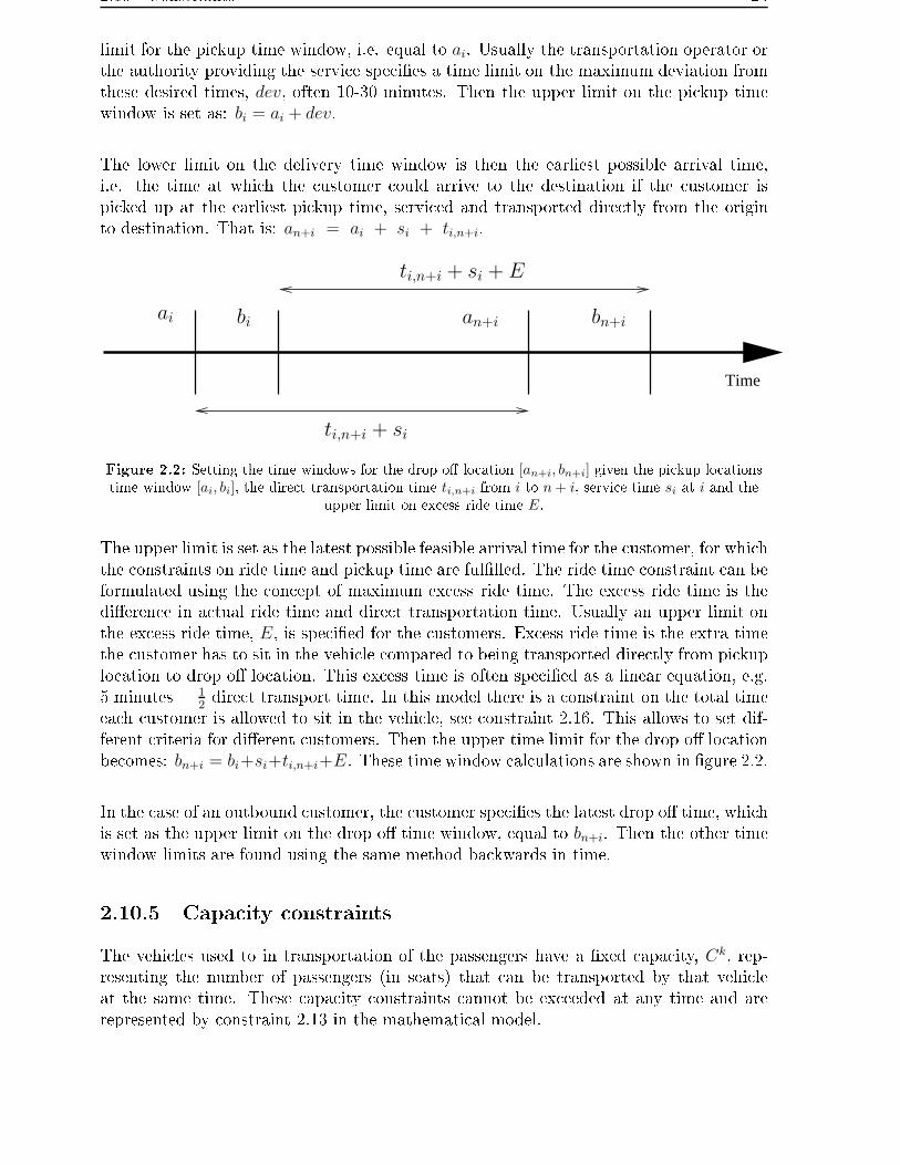
The lower limit on the delivery time window is then the earliest possible arrival time,i.e. the time at which the customer could arrive to the destination if the customer ispicked up at the earliest pickup time, serviced and transported directly from the originto destination. That is: an+i = ai + si + ti,n+i.
Time
ti,n+i + si
bi bn+i
ti,n+i + si + E
ai an+i
Figure 2.2: Setting the time windows for the drop o� location [an+i, bn+i] given the pickup locationstime window [ai, bi], the direct transportation time ti,n+i from i to n + i, service time si at i and the
upper limit on excess ride time E.
The upper limit is set as the latest possible feasible arrival time for the customer, for whichthe constraints on ride time and pickup time are ful�lled. The ride time constraint can beformulated using the concept of maximum excess ride time. The excess ride time is thedi�erence in actual ride time and direct transportation time. Usually an upper limit onthe excess ride time, E, is speci�ed for the customers. Excess ride time is the extra timethe customer has to sit in the vehicle compared to being transported directly from pickuplocation to drop o� location. This excess time is often speci�ed as a linear equation, e.g.5 minutes + 1
2direct transport time. In this model there is a constraint on the total time
each customer is allowed to sit in the vehicle, see constraint 2.16. This allows to set dif-ferent criteria for di�erent customers. Then the upper time limit for the drop o� locationbecomes: bn+i = bi+si+ti,n+i+E. These time window calculations are shown in �gure 2.2.
In the case of an outbound customer, the customer speci�es the latest drop o� time, whichis set as the upper limit on the drop o� time window, equal to bn+i. Then the other timewindow limits are found using the same method backwards in time.
2.10.5 Capacity constraints
The vehicles used to in transportation of the passengers have a �xed capacity, Ck, rep-resenting the number of passengers (in seats) that can be transported by that vehicleat the same time. These capacity constraints cannot be exceeded at any time and arerepresented by constraint 2.13 in the mathematical model.

26 Chapter 2. Dial a ride problem
Loads on vehicles
In order to keep track of the number seats needed for the passengers in each vehiclethroughout the route the term of load for each vehicle is introduced. Load of vehicle at apoint in time is the number of seats needed for the passengers in the vehicle at that pointin time. When a vehicle has serviced a pickup location i the change in load is representedby li = demi and the change in load after servicing a drop o� location n+i is ln+i = −demi.
The actual load of a vehicle k after servicing a location i is Lki . The load of the vehicle
after servicing the next location in the route, j, is then Lkj = Lk
i + lj . In order to calculatethe load in this manner constraint 2.12 is introduced to the model. It ensures that theloads are correctly calculated for the edges used in the route. The actual loads of thevehicles are set to zero at the depots in constraint 2.14.
2.10.6 Linearization of constraints
Note that constraints 2.9 and 2.12 are non-linear constraints. They can be linearized,which is necessary if an LP-solver is to be used to solve the problem. The linearizationof constraint 2.9 can be performed in the following way:
xki,j(T
ki + si + ti,j + W k
j − T kj ) ≤ 0 (2.18)
is equivalent toT k
i + si + ti,j + W kj − T k
j −M(1− xki,j) ≤ 0 (2.19)
where M is a large number and recall that xki,j is binary.
Constraint 2.12 can also be linearized. First the constraint needs to be replaced by twoinequality constraints, which combined are equivalent to the equality constraint 2.12. Thetwo inequalities are:
xki,j(L
ki + lj − Lk
j ) ≤ 0 (2.20)
xki,j(L
ki + lj − Lk
j ) ≥ 0 (2.21)
The linearization of the two inequalities 2.20 and 2.21 is performed in the same manneras is shown above for constraint 2.9.
2.11 Related problems
It is very useful to study the problems that are related to the DARP and the solutionmethods used to solve the related problems. Solution methods that give good results fora related problem can be expected to give good results for the DARP as well.
The travelling salesman problem (TSP) gets its name from a salesman who has todrive from door to door to visit his prede�ned customers trying to sell his merchandise.He leaves his house, visits all the customers and returns back to his home after the work

2.11 Related problems 27
is performed. He, of course, wants to return home as early as possible. The length of theworkday of the salesman is determined by the order of the visits to the customers. In thisstatement we are taking two assumptions. The �rst assumption is that the travelling timebetween any two customers is not time dependent, i.e. the travelling time is the same inthe morning, afternoon or night. The second assumption states that the travelling timebetween any two customers is independent on the order of the customers, i.e. travellingtime from customer i to customer j is the same as the travelling time from customer j tocustomer i. The TSP is then to �nd the route in which all the customers are visited withthe minimum total travel time.
Of course the TSP can be generalized to �t other systems in which it is necessary to getfrom a base location, visit other locations once and only once and end at the base again.The problem stated more generally is then to �nd a route for a vehicle which visits eachof n prede�ned locations once and only once and minimizes the total travel time. Thetravel time is dependent on the speed of the salesmans vehicle and the speed can vary,e.g. on di�erent types of roads, and therefore it is often the travelling distance that isminimized instead of travel time in TSP. It seems easy to solve such a problem but ifthere are n locations to visit there are (n− 1)! possible solutions to the problem.
This is the classical travelling salesman problem. Additional constraints and speci�cationscan be added to the problem, as in the vehicle routing problem (VRP). In VRP morethan one vehicle is available to visit the locations and each of the vehicles has a limitedidentical capacity. The home of the vehicles is called a depot, from where the vehiclesstart and end their route. There can be more than one depot and each having a certainnumber of vehicles available to visit the locations. Each vehicle is either making deliveriesto customers or picking up goods from vendors/plants - not both. Each customer is tobe serviced by exactly one vehicle, it is for example not possible for a vehicle to deliverthe customer half of the ordered goods and then another vehicle to bring the rest of theorder. In this problem the vehicles have a capacity and the distance between customersis known. There can be an upper limit on the length of routes of the vehicles and thedemand/supply at each location is known. The vehicle routing problem consists of allo-cating customers to vehicles and �nd the order in which each vehicle visits its customerso the total travelling distance of all vehicles serving all customers is minimized whilemaintaining all the constraints.
In the vehicle routing problem with backhauls (VRPB), which is an extension ofVRP, the set of customers is partitioned into two subsets: Linehaul and Backhaul cus-tomers. Each Linehaul customer requires the delivery of a given quantity of product fromthe depot, whereas a given quantity of product must be picked up from each Backhaulcustomer and transported to the depot. First all the deliveries in the same route must bemade and then the pickups in the same route take place, so as to avoid rearranging thegoods in the vehicle.
The pickup and delivery problem (PDP), also called the vehicle routing problemwith pickup and delivery (VRPPD), is a VRP with the addition that there is a pickup anda delivery location given for each transportation request. So that a vehicle has to drive to
28 Chapter 2. Dial a ride problem
a pickup location to pickup goods and then later in the route drive to the correspondingdrop o� location to deliver the goods that are stored in the vehicle. In other respectsthere is no other modi�cations from the VRP described above.
All the problems described above deal with the transport of goods, so issues as how longthe goods are in the vehicle are o� no or insigni�cant importance and we can disregardit. This is however not the case with the dial-a-ride problem, since it usually dealswith the transportation of people. That fact complicates things considerably, since serviceprovided to customers now has to be taken into account. Apart from that the dial-ride-problem is the same problem as PDP described above.
To all the problems described above time window constraints associated with each/someof the locations to be visited can be added. Time windows constitutes a time interval inwhich one is allowed to visit a speci�c location. For example, if the time window for cus-tomer 3 is [8, 9] it means that the transporting vehicle can deliver/pickup goods between8 and 9 o'clock. The time windows can be hard constraints, that is if the vehicle does notarrive within the speci�c time interval it either has to wait, if early, or if late, then thevehicle is not allowed to stop there. Soft time windows allow for visits outside the speci�ctime window but at an extra cost.
The last problem described here is the bin-packing problem. The bin-packing problemis the problem of packing a set of objects into a number of bins2 such that the total weightor volume does not exceed some maximum value. The objective is to arrange the itemsin such a way that the number of bins used is minimized.
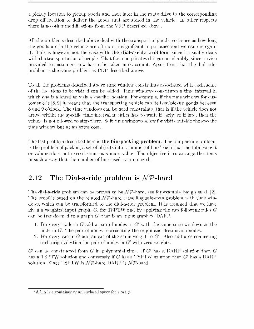
2.12 The Dial-a-ride problem is NP-hardThe dial-a-ride problem can be proven to be NP-hard, see for example Baugh et al. [2].The proof is based on the related NP-hard travelling salesman problem with time win-dows, which can be transformed to the dial-a-ride problem. It is assumed that we havegiven a weighted input graph, G, for TSPTW and by applying the two following rules Gcan be transformed to a graph G′ that is an input graph to DARP:
1. For every node in G add a pair of nodes in G′ with the same time windows as thenode in G. The pair of nodes representing the origin and destination nodes.
2. For every arc in G add an arc of the same weight to G′. Also add arcs connectingeach origin/destination pair of nodes in G′ with zero weights.
G′ can be constructed from G in polynomial time. If G′ has a DARP solution then Ghas a TSPTW solution and conversely if G has a TSPTW solution then G′ has a DARPsolution. Since TSPTW is NP-hard DARP is NP-hard.
2A bin is a container or an enclosed space for storage.

Chapter 3
Previous Work
Study of the dial-a-ride problem started in the late 1960s. Since then several versionsof the dial-a-ride problem have been proposed and several techniques used to solve theproblem.
In this chapter a short description of some of the papers that have been published onusing heuristics for solving the static multi-vehicle dial-a-ride problem with time windowsis presented. Firstly there will be a description of a paper in which the problem is solvedusing a heuristic algorithm based on insertion. Secondly an introduction of two papersthat use meta-heuristics; simulated annealing, and tabu search, to solve the problem isgiven. A discussion of using the genetic algorithm for solving the related problem ofpickup and delivery with time windows and the vehicle routing problem is presented. Thechapter will be concluded by a comparison of the papers along with a discussion of theirin�uence on this project.
3.1 Jaw et al.
The work performed by Jaw et al. [9] in 1986 is a pioneer research within the area of dial-a-ride and most of the following research performed in this area is based on their work.In the paper a sequential insertion heuristic algorithm for solving the static dial-a-rideproblem is described. The algorithm is referred to as ADARTW.
In the algorithm customers are �rst sorted according to their earliest pickup time. Thenthe algorithm tries to assign the customer on the top of the list to a vehicle, that isthe customer found to have the earliest pickup time. The assignment is performed byconsidering the additional cost of all feasible insertions of the customer to a vehicle andthe cheapest insertion is chosen. If the customer cannot be assigned to existing vehiclesthe customer is either rejected or a new vehicle initialized. The algorithm continues toprocess customers in sequential order according to the list, until the last customer on thelist has been processed.
29

30 Chapter 3. Previous Work
Each customer either has to give a desired pickup time or a desired delivery time. Timewindows are then calculated given:
• the desired times,• the direct ride time from origin to destination for each customer,• the maximum acceptable ride time for each customer, which is a linear function ofthe direct ride time,• the maximum acceptable deviation from the desired pickup or delivery time for eachcustomer.
The objective function combines the minimization of operator costs and the minimizationof customer inconvenience with respect to both customer ride time and deviation fromdesired pickup or delivery times speci�ed by each customer. The di�erent parts of theobjective function are balanced by multiplying them by user-speci�ed constants. Thevalues of the constants are then varied in the computational experiments.
In the computational experiments the ADARTW algorithm was run on a number ofsimulated data sets with 250 customers and 4 to 5 vehicles and real data sets with 2617customers and 28 vehicles. The CPU time for the simulated data set was about 20seconds and about 12 minutes for the real data set. The authors conclude that theircomputational experience shows that the ADARTW algorithm gives at least as good asor superior solutions to those encountered in manual planning in all respects.
3.2 Baugh et al.
In 1998 Baugh et al. [2] presented a paper in which the meta-heuristic algorithm, simulatedannealing, is used for solving the static dial-a-ride problem. The authors argue thatit is wise to use simulated annealing for solving the problem since it is easily adaptedto problems with a well de�ned neighbourhood structure, it has desirable theoreticalconvergence properties and it can easily be combined with other meta-heuristics, such astabu search.
The work is based on the classical cluster-�rst, route-second approach. A cluster is agroup of customers assigned to the same vehicle and also serviced together. Customersare �rst organized into clusters and then the routes are developed for each individual clus-ter. In this paper the clustering is performed using simulated annealing while the routingis performed using a modi�ed space-time nearest neighbour heuristic. The authors claimthat the clustering is the most vital part of the process since routing only involves a smallset of customers and therefore it is not necessary to solve the routing problem with analgorithm as sophisticated as one used for clustering.
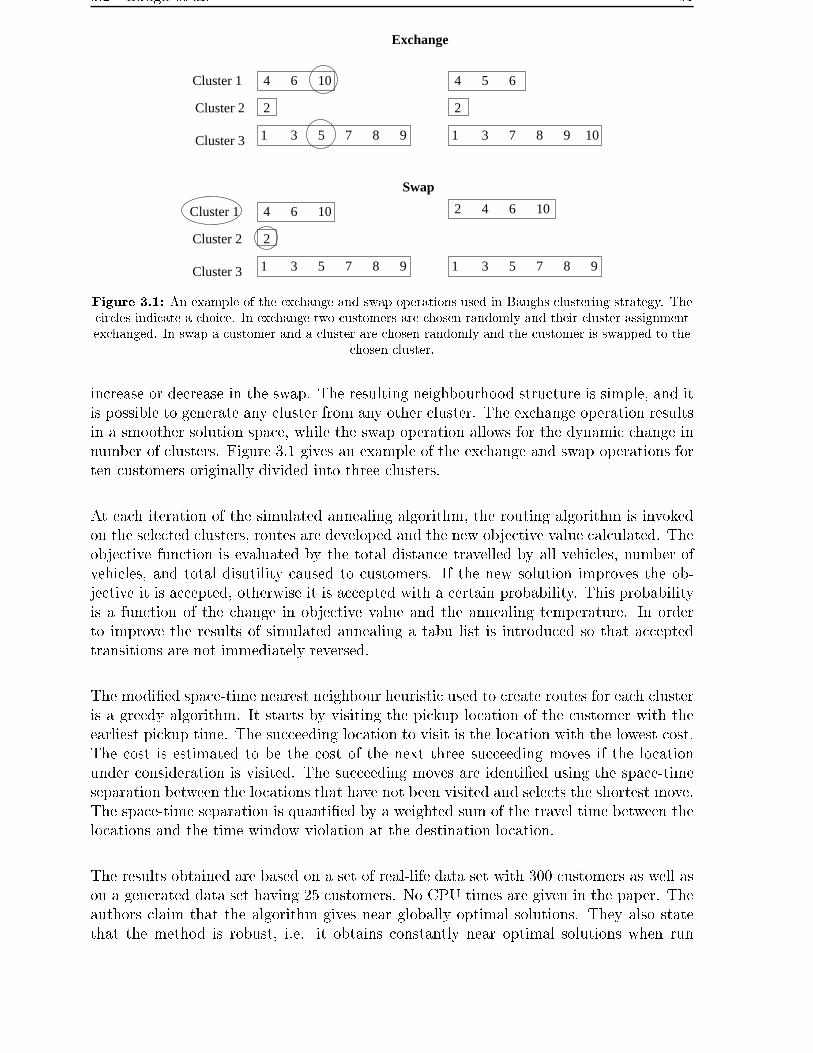
The clustering algorithm is initialized by assigning customers to clusters randomly. Twooperations are then used to alter the current clustering of customers. Either two customersare randomly chosen and their current clusters are exchanged, leaving the total numberof clusters unchanged. Alternately, a customer and a cluster are randomly selected, andthe customer is swapped to the selected cluster, as a result the number of clusters can
3.2 Baugh et al. 31
1 3 5 7 98
2
4 6 10
2
4 5 6
1 3 7 8 9 10
Cluster 1
Cluster 2
Cluster 3
1 3 5 7 98
2
4 6 10
1 3 5 7 98
2 4 6 10Cluster 1
Cluster 2
Cluster 3
Swap
Exchange
Figure 3.1: An example of the exchange and swap operations used in Baughs clustering strategy. Thecircles indicate a choice. In exchange two customers are chosen randomly and their cluster assignmentexchanged. In swap a customer and a cluster are chosen randomly and the customer is swapped to the
chosen cluster.
increase or decrease in the swap. The resulting neighbourhood structure is simple, and itis possible to generate any cluster from any other cluster. The exchange operation resultsin a smoother solution space, while the swap operation allows for the dynamic change innumber of clusters. Figure 3.1 gives an example of the exchange and swap operations forten customers originally divided into three clusters.
At each iteration of the simulated annealing algorithm, the routing algorithm is invokedon the selected clusters, routes are developed and the new objective value calculated. Theobjective function is evaluated by the total distance travelled by all vehicles, number ofvehicles, and total disutility caused to customers. If the new solution improves the ob-jective it is accepted, otherwise it is accepted with a certain probability. This probabilityis a function of the change in objective value and the annealing temperature. In orderto improve the results of simulated annealing a tabu list is introduced so that acceptedtransitions are not immediately reversed.
The modi�ed space-time nearest neighbour heuristic used to create routes for each clusteris a greedy algorithm. It starts by visiting the pickup location of the customer with theearliest pickup time. The succeeding location to visit is the location with the lowest cost.The cost is estimated to be the cost of the next three succeeding moves if the locationunder consideration is visited. The succeeding moves are identi�ed using the space-timeseparation between the locations that have not been visited and selects the shortest move.The space-time separation is quanti�ed by a weighted sum of the travel time between thelocations and the time window violation at the destination location.
The results obtained are based on a set of real-life data set with 300 customers as well ason a generated data set having 25 customers. No CPU times are given in the paper. Theauthors claim that the algorithm gives near globally optimal solutions. They also statethat the method is robust, i.e. it obtains constantly near optimal solutions when run

32 Chapter 3. Previous Work
on the test problems. Furthermore it is noted that a minimal user input for �ne tuningannealing parameters are needed.
3.3 Cordeau and Laporte
In 2003 Cordeau and Laporte [4] wrote a paper which describes how a tabu search heuris-tic is used for solving the static dial-a-ride problem. Their algorithm starts with an initialsolution that is randomly generated. In each iteration the best solution in the neighbour-hood of the current solution is chosen. In order to avoid cycling, solutions possessingsome attributes of recently visited solutions, are put on the tabu list and are thereforeforbidden for a number of iterations unless they constitute a new incumbent. It is al-lowed to explore infeasible solutions during the iterations. That is performed by relaxingthe constraints in the problem, by adding new terms into the objective function, each ofwhich represents an evaluation of the violation of one constraint multiplied by a positiveparameter. After each iteration the parameters are adjusted so that currently violatedconstraints get more weight in the objective function and the weights are reduced on con-straints that are ful�lled by the current solution. The objective function consists of thetotal transportation cost of the vehicles and the violation terms (customer inconvenienceis a part of the violation terms).
The initial solution is constructed by randomly assigning the customers requests to vehi-cles, and the order of the requests in each vehicles route is the same as the order in whichthey were assigned to the vehicle. The origin of each request comes �rst and then thedestination.
The neighbourhood of the current solution is constructed using a simple operator thatreassigns a request to a new vehicle in the current solution. Now the di�erence betweenthe new solution and the old solution is restricted to two routes. The order of requestsin the two routes is the same as before, but in one of the routes one request is missingwhile in the other one the same request has been inserted in the route in such a way,that the total increase in total cost for this solution is minimized. The cost for a solutionequals the objective function value for the solution. Routes are optimized every time anew best solution is identi�ed, and also systematically during the iteration process. Thisis performed by intra route exchanges. In the intra route exchanges every customer isremoved from its current route and the pickup and drop o� locations are reinserted intothe route in the best possible positions. The best possible position is the position thatminimize the objective function value.
In this algorithm, it is possible to use the full algorithm to evaluate candidate solutionsin the neighbourhood. The full algorithm consists of eight steps and in those steps timewindow violations, route duration and ride times are minimized. It is also possible totake the �rst six steps, which minimizes time window violations and route duration, andto perform the �rst two steps and only minimize the time window violations. The threedi�erent approaches were tested using both randomly generated data sets with 24 to 144customers and six real-life data sets containing either 200 or 295 customers. The CPU

3.4 Jih et al. 33
times for the randomly generated data sets are about 2 minutes for the smallest data setsand up to 93 minutes for the largest data sets. The CPU times for the real-life data setsare given to be about 13 to 268 minutes. The conclusion is that the full version of thealgorithm reviled the best solutions but is the most expensive in CPU-time. The resultsgiven in the paper are not compared to results obtained by others.
3.4 Jih et al.
Jih et al. [10] published a paper in 2002 on solving the single vehicle pickup and deliveryproblem with time windows using a family competition genetic algorithm.
When using the genetic algorithm it is necessary to have a chromosome representationof a route and that is performed by letting the chromosome represent the locations in atravelling sequence of the route.
The algorithm is allowed to explore infeasible solutions during the iterations process. Theobjective function, in GA-germs also known as the �tness function, is the summation ofthe total travel cost of the vehicle and the penalty for violating constraints, which is thecase with infeasible solutions.
The family competition genetic algorithm is based on the genetic algorithm with the ex-tension that every individual also owns its family. When creating a new generation eachindividual in the current population is set to be a family father. Each family father is usedto create a new family by recombining the family father and randomly chosen alternativeparents from the population. The recombining is called a crossover in GA terms. Thecrossover can be followed by a mutation, which is usually a small random change of asolution. The size of a family is a constant kf . In each iteration kfM new individuals arecreated, where M is the population size. Only the best individual in a family survivesand becomes a member of the new population. The iterations will run until a termina-tion condition is reached. In the termination condition, used in the experiments that arepresented, is not stated.
Two types of operators are used to change the current solution: Crossover and muta-tion. Four di�erent types of crossover are considered; the order-based crossover, uniformorder-based crossover, merge cross #1, and merge cross #2. The �rst two are traditionalcrossover operators but the last two use a global precedence vector to give guidance in thecrossover. Two mutation operators are considered. The �rst one selects two random genesand interchanges their position, while the second one chooses randomly two cut sites andthe order of the sub-routes is inverted. Mutation is used in this algorithm if a child andone of its parents represent the same route. The reason for this choice is that it supportsroute diversity and prevents the search space to become bound in a local optimal solutions.
The algorithm is run on randomly generated data sets with up to 100 customers andthe CPU time is about 38 minutes for the largest data sets. In the experiments the

34 Chapter 3. Previous Work
family competition genetic algorithm is compared to the traditional genetic algorithm.The authors found that the �rst one results in better solutions and the probability ofobtaining the best solution is higher at similar running times. The di�erent types ofcrossover operations are also compared and the order-based crossover is found not to besuited for the pickup and delivery problem. It is found that the uniform order-basedcrossover gives the best solutions but requires much execution time while both types ofthe merge crossover are faster but give reasonably good solutions and might therefore bebetter suited for real-time approach. The main conclusion is that the family competitiongenetic algorithm succeeded in �nding feasible solutions to the generated problems inreasonable time and that the choice of modifying operators greatly in�uences the resultsof the algorithm. The results of the algorithm are compared with the optimal valueswhich are available for the smaller data sets (up to 40 customers). The best results forthe family competition genetic algorithm is by using the uniform order-based crossover isable to reach the optimum on the average in 83% of the runs for the data sets with up to40 customers.
3.5 Pereira et. al
The paper written by Pereira et. al [13] is called: �GVR: a New Genetic Representationfor the Vehicle Routing Problem.� In the paper the genetic algorithm is used to solve thecapacitated VRP. A two-level schema (GVR) is designed to represent all the information apotential solution must encode. A potential solution must specify the number of vehiclesrequired, allocation of customers to vehicles and the order of customers in the route ofeach vehicle.
An individual represents a solution and is made of a chromosome. The genes in the chro-mosome are the customers in their visiting order. Each customer must be representedexactly once in the individual. If capacity of the vehicles is exceeded in any route, theroute is split up into smaller routes, i.e. new vehicles are added to the solution, untilcapacity is within limits, at the interpretation level.
The algorithm proceeds from an initial population of n individuals. In each iterationthere are chosen n parents and n o�springs created using genetic operators. Two typesof operators are considered: Crossover and mutation. The operators should be capable ofchanging the order of customers within routes, modifying the allocation of customers tovehicles and altering the number of routes in solution. The o�spring must also represent alegal solution. A legal solution is a solution in which each customer is assigned to exactlyone vehicle. The capacity of the vehicles is not an issue since it is assumed that thecapacity constraint is checked and �xed at interpretation level.
In the crossover an o�spring is created by inserting a fragment of genetic material (asub-route) from one parent into one line of the chromosome (route) of the other parent.The placement of the insertion is directly behind a customer that is not a part of thesub-route and is closest to the �rst customer in the sub-route. Afterwards duplicatesin other chromosomes are removed. An example of how the crossover works is given in

3.5 Pereira et. al 35
Route 2
5610
732
Route 2
Route 1
Route 2
Route 1 56872
56
7
Route 3
10
9 41
419
419
OffspringSub−route from Individual 2
Individual 2
Individual 1
10
8
3
2
1
839
4Route 1
Figure 3.2: An example of the crossover used by Pereira et al. An o�spring is created by selecting asub-route from parent 2, inserting it into parent 1 and removing duplicates. Here it is assumed
customer 6 is closest to customer 9.
�gure 3.2. In the �gure individual 1 and 2 have been chosen as parents. A sub-route israndomly selected from individual 2. The customer that is geographically closest to the�rst customer (6) in the sub-route and is not a part of the sub-route is identi�ed (9).The sub-route is inserted into individual 1 and the placement is directly behind customer9. The customers that originally belonged to individual 1 and are now duplicates of thecustomers in the sub-route are removed from the o�spring. The crossover is capable ofreducing the number of routes, changing the order of customers in routes and reallocatingcustomers to routes. It is however not possible to add new routes to the solution.
The o�springs can be mutated after the crossover. In this paper there are four mutationoperators. First, two customers can be swapped within the same route or di�erent routes.Second, routes can be inverted, i.e. the visiting order of customer is inverted. Third, acustomer is selected and inserted in another place, possibly creating a new route contain-ing only this customer. Fourth, a sub-route is chosen and inserted in another randomplace, both intra or inter-displacement are a possibility. The fourth mutation operatoris very similar to the crossover, the only di�erence is the selection of insertion placementof the sub-route. In the crossover it is behind the geographically closest customer but inthe mutation it is chosen randomly. The mutation operator is therefore capable of addingand deleting routes, altering order and allocation of customers.
The algorithm is tested on a collection of data sets with 12 instances from some well-known benchmarks1. The results show that the method is very e�cient for solving thisproblem. The authors are able to �nd reach the best solutions that have been found formost instances of the well-known benchmarks or be very close to the best. They are evenable to �nd new best solutions to some of the test instances. The method proved to berobust, i.e. parameter settings do not a�ect the quality of the solutions obtained. NoCPU times are given in the paper. It is however concluded that the results are to beconsidered preliminary.
1Augerat Set A, Augerat Set B and Christo�des and Elion
36 Chapter 3. Previous Work
3.6 Comparison
In this section a comparison of the papers, which have been described previously in thischapter, will be presented. There will also be a discussion of the ideas and inspirationthat these papers have had on the work described in this project.
The �rst paper is written by Jaw et al. in 1986. The paper describes a pioneeringwork performed in the area of the dial-a-ride problem. A sequential insertion heuristicalgorithm to solve the static dial-a-ride problem is proposed. In this algorithm the cus-tomers are sorted according to their earliest pickup times. The algorithm is used to solverandomly generated test instances with up to 250 customers in about 20 seconds andreal-life data sets with 2617 customers in about 12 minutes. The results of the real-lifedata sets are compared with results from manual planning and concluded that the solu-tion method gives as good as or superior solutions to the solutions obtained by manualplanning.
The paper is, in my opinion, very clearly written and interesting. It explained very wellthe time windows calculations and the complications involved in the dial-a-ride problem.
The second paper, written by Baugh et al. in 1998, describes how the DARPis solved using simulated annealing to group customers thereafter a space-time nearestneighbour heuristic is used to make routes for each group. To improve the performanceof the simulated annealing schema, a tabu list is included. The simulated annealing isused to solve randomly generated test instances with up to 25 customers and real-lifedata sets with up to 300 customers but no CPU times are given. The results obtainedfor the real-life data sets are compared to the plans used in practice. The results ob-tained by Baugh et al. outperformed the plans used in practice. It should however benoted that the plans are not optimal and include several policies that are not modeledby Baugh et al. Therefore I conclude that it is impossible to conclude about the qualityof the solutions obtained. The authors do however claim that the algorithm is capableof giving near globally optimal solutions but that is not shown explicitly. The algorithmis further claimed to be robust, i.e. obtains constantly good optimal solutions, and torequire minimal user input for �ne tuning the parameters needed in the algorithm.
The paper is very well written. The terms used in the paper are clearly and preciselyexplicated. As an example a mathematical model of the dial-a-ride problem is presented,which is not seen in many papers on the subject. Parts of that model are used in themathematical model presented in this project. The ideas of clustering and routing will beused in solution method and the routing heuristic presented in the paper lays the founda-tion for the routing heuristic used in this project. It is however questionable whether it iswise of the authors to use simulated annealing with a tabu list instead of simply using thetabu search heuristic. The fact that the authors do not give CPU times and explain howthey come to the conclusion that their algorithm is able to give near optimal solutionsdecreases the credibility of the paper in my opinion.

3.6 Comparison 37
The third paper is written by Cordeau and Laporte in 2003. There is a descrip-tion of how a tabu search heuristic can be used to solve the DARP. The method is testedon several randomly generated data with up to 144 customers in abut 93 minutes setsalong with some real-life data sets with up to 295 customers in 268 minutes. The resultsare not compared to results obtained by others and only the cost is presented as a resultfor each data set.
The paper is not as well written as the previous ones. It is harder to understand thepaper and catch precise information details. Furthermore, in the results chapter there isalso only reported the cost for the best solutions found and the results not compared withresults from others. Consequently it is impossible to compare the results with results inthe previous papers. However an Internet address where all the data is available alongwith more detailed results is given. It is excellent that the test cases are available forothers to use as to being able to compare results and it is perhaps the beginning of adatabase of standard dial-a-ride problems. All the test cases that will be used in thisproject are received from this Internet site.
The fourth paper, written by Jih et al. in 2002, gives a description of how afamily competing genetic algorithm is used to solve the single vehicle pickup and deliveryproblem. The algorithm is used to solve randomly generated data sets with up to 100customers using up to 38 minutes. For the smaller data sets the algorithm is able to �ndthe optimum with a probability of 83% on the average. The conclusion of the authorsis that the family competing genetic algorithm succeeds in �nding feasible solutions inreasonable time.
The paper is very interesting but very sparse in its description of the methods used tosolve the problem. Also only the single vehicle PDP with time windows is solved and it isnot clear how to extend the method to the multi vehicle case. The paper gave inspirationand ideas of how to use the GA in solving the dial-a-ride problem at the initial stages ofthe working process of this project.
The �fth paper is written by Pereira et al. in 2002. Here an analysis of how thegenetic algorithm is used to solve the vehicle routing problem is presented. A descrip-tion of a two level representational schema is given. The schema is constructed in orderto incorporate all the information that a candidate solution must encode. Experimentalresults show the method to be both e�ective and robust as well as capable of discoveringnew best solutions to some well-known benchmarks but no CPU times are given.
This paper is very well written. There are many examples and illustrations of how thealgorithm works. The two level representational schema and the crossover operators pre-sented in the paper gave an inspiration of how to use the genetic algorithm for solvingthe DARP presented in this project.
The �rst three of the papers using di�erent solution methods to solve the static dial-a-rideproblem. The formulation of the DARP is not the same in the papers and they use di�er-
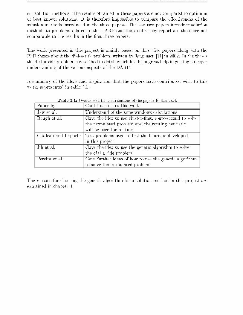
38 Chapter 3. Previous Work
ent solution methods. The results obtained in these papers are not compared to optimumor best known solutions. It is therefore impossible to compare the e�ectiveness of thesolution methods introduced in the three papers. The last two papers introduce solutionmethods to problems related to the DARP and the results they report are therefore notcomparable to the results in the �rst three papers.
The work presented in this project is mainly based on these �ve papers along with thePhD theses about the dial-a-ride problem, written by Jørgensen [11] in 2002. In the thesesthe dial-a-ride problem is described in detail which has been great help in getting a deeperunderstanding of the various aspects of the DARP.
A summary of the ideas and inspiration that the papers have contributed with to thiswork, is presented in table 3.1.
Table 3.1: Overview of the contributions of the papers to this work
Paper by: Contributions to this work
Jaw et al. Understand of the time windows calculationsBaugh et al. Gave the idea to use cluster-�rst, route-second to solve
the formulated problem and the routing heuristicwill be used for routing
Cordeau and Laporte Test problems used to test the heuristic developedin this project
Jih et al. Gave the idea to use the genetic algorithm to solvethe dial-a-ride problem
Pereira et al. Gave further ideas of how to use the genetic algorithmto solve the formulated problem
The reasons for choosing the genetic algorithm for a solution method in this project areexplained in chapter 4.

Chapter 4
Solution method
In this chapter a description of the solution method used to solve the dial-a-ride prob-lem formulated in chapter 2 is given. The solution method is based on the cluster-�rst,route-second principle. A genetic algorithm is developed for solving the clustering andthe modi�ed space-time nearest neighbour heuristic developed by Baugh et al. [2] is usedin an adjusted version for solving the routing.
The chapter starts by a description of the decision process of choosing the solution method.Next the genetic algorithm will be described containing a discussion on the important is-sues to consider when constructing the genetic algorithm, such as solution representation,population size, construction of initial population, �tness calculations, selection mech-anism and which modifying operators to chose. The two types of modifying operatorsaddressed are crossover and mutation. Thereafter the modi�ed space-time nearest neigh-bour heuristic will be described.
4.1 Choosing the solution method
The choice of solution method for solving the dial-a-ride problem depends on solutiontechniques considerations (such as existing algorithms in the available literature), avail-able computer software, computer/hardware and time.
In order to limit the search for existing algorithms to solve the problem, it is �rst consid-ered whether to use exact or heuristic algorithms. Lets start by comparing the two typesof algorithms.
When solving an optimization problem we are really only optimizing a model of a problemoriginating in the real-world. There is no guarantee that the best solution to the model isalso the best solution to the underlying real-world problem. Two reasons for why the bestsolutions do not match are that some real-world constraints can be decided to be omittedin the model, because they are not considered important, and the numbers used in themodel/implementation are not be precise to the last digit (e.g. π and measurements).Even though heuristics are not guaranteed to provide us with an optimal solution to the
39

40 Chapter 4. Solution method
underlying problem then neither are exact methods. Furthermore heuristic methods areusually more �exible and capable of coping with more complicated and realistic objec-tive functions and/or constraints than exact algorithms. Another reason for consideringheuristics for solving the dial-a-ride problem is the NP-hardness of the DARP, see sec-tion 2.12, which makes the problem solvable using exact algorithms only for small problemsizes.
In Baugh et al. [2] alternative mathematical programming approaches are explored forsolving a practical DARP. Three mixed-integer linear programming models (MILP) aretested and it concluded that the largest problem size that can be solved using commercialoptimization packages is about 10 customers. The MILP is solved using a custom branch-and-bound solver and it is observed that for problem sizes larger than 15 customers even�nding any feasible integer solution proves to be di�cult. A dial-a-ride system consistingof 15 customers is small compared to a realistic system of around 200-300 customers.
Next we need to consider which heuristic algorithm to use. As we can see in Cordeauand Laport [4] as well as in Baugh et al. [2], meta-heuristics work well when solving thedial-a-ride problem. According to Jih et al. [10] the genetic algorithm (GA) is a goodapproach for solving NP-hard problems and in particular the related travelling salesmanproblem and vehicle routing problem.
One of the main objectives of this project is to experiment with a new solution methodfor the dial-a-ride problem and the GA has not previously been used for solving the DARP.
Since the GA is considered to be a good approach for solving routing problems and has notbeen used for solving the DARP it is decided to investigate the behaviour of the geneticalgorithm when used for solving the dial-a-ride problem formulated here. The originalidea is solving the problem in one step using a sequential two-level chromosomes repre-sentation, similar to the one used in Pereira [13]. In the chromosome representation bothcustomers allocation to vehicles and the order of customers in the routes of the vehicles areencoded. The chromosome representation is used for solving the vehicle routing problembut the extension to the dial-a-ride problem is problematic. The main problem is to checkif the precedence constraint is kept. In order to solve this problem some elaborate �x-upprocedure would have to be initialized each time a new individual is created. That is acomplicated and time consuming process so other ideas are considered. The idea of thecluster-�rst, route-second strategy comes to mind inspired by papers written by Baughet al. [2] and Toth and Vigo [17]. In the papers the cluster-�rst, route-second solutionmethod is described, and Baugh et al. applies it to the DARP while Toth and Vigo applyit to the VRPB. The cluster-�rst, route-second strategy bears some similarities to thebin-packing problem. In the bin-packing problem objects are to be packed into a numberof bins, that is the objects are organized into clusters, one for each bin. The way theobjects are arranged into the bins can be decided simultaneously or decided after the ob-jects have been clustered. This is the same idea as the cluster-�rst, route-second in DARP.
The cluster-�rst, route-second is a strategy that partitions the entire set of customers into

4.2 The Genetic Algorithm 41
clusters. All the customers belonging to the same cluster are serviced by the same vehicle.Routes are thereafter developed for the individual clusters.
Based on the good experience with the cluster-�rst, route second strategy reported byothers [2] on similar problems it is decided to use cluster-�rst, route-second solution ap-proach. First it is considered using the GA for both clustering and routing, but since theGA behaves in a random manner it seemed like a better idea to use the GA for one partand another more deterministic method for the other part of the solution method. Themost crucial decision for DARP is the allocation of customers to vehicles. Therefore it isvital to use a good global solution technique, such as the GA, in that part of the problemwhile the routing can be solved by a faster heuristic. Very good heuristics algorithmsfor solving the routing problem to near optimality exist, such as the Lin-Kernighan al-gorithm [2]. Note however that the routing problems are expected to be small, typicallythe number of customers in a route is expected to be of the order 10 or 20. The modi�edspace-time nearest neighbour heuristic by Baugh et al. should give good solutions withminimal computational requirements [2].
The problem will be solved usingthe genetic algorithm for clustering and
a modi�ed space-time nearest neighbour heuristic for routing
4.2 The Genetic Algorithm
The main ideas behind the genetic algorithm are taken from biology. Terms such as nat-ural selection and the survival of the �ttest lie at the core of the genetic algorithm (GA).In the GA, a population of individuals is created, each individual represents a candidatesolution to the problem. Such a candidate solution is represented by a string of numbers,similar to the genetic representation of chromosomes for living organisms. So an individ-ual is represented by its genetic material.
The individuals are paired and o�springs produced, that is, new candidate solutionsare created using existing solutions. The selection of individuals to pair and produceo�springs is based on the �tness of the individuals, i.e. the �tter the individual is, thehigher probability of the individual to be allowed to produce o�springs. The �tness valuesof individuals are usually proportional to the corresponding objective function value ofthe solution the individual represents. The individuals used to produce an o�spring arecalled parents. The new o�springs are created using some kind of genetic operators. Thetwo most common genetic operators are crossover and mutation.
• CrossoverCrossover is the main genetic operator and is applied to pairs of individuals. Incrossover, an o�spring is created by combining the genetic material of two existingsolutions, e.g. the �rst part of one parent chromosome and the last part of the
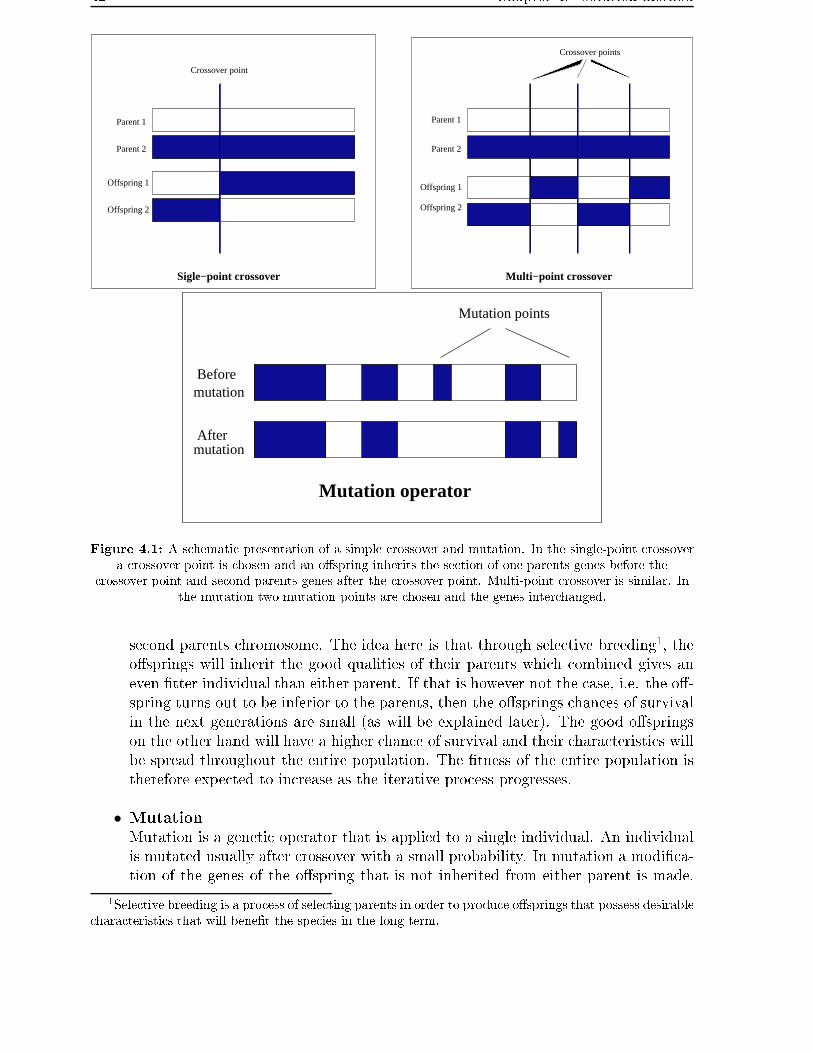
42 Chapter 4. Solution method
��������������������
��������������������
���
���
������������
������������
Offspring 2
Offspring 1
Parent 2
Parent 1
Crossover point
Offspring 2
Offspring 1
Parent 2
Parent 1
Sigle−point crossover Multi−point crossover
Crossover points
Mutation operator
Mutation points
mutationBefore
mutationAfter
Figure 4.1: A schematic presentation of a simple crossover and mutation. In the single-point crossovera crossover point is chosen and an o�spring inherits the section of one parents genes before the
crossover point and second parents genes after the crossover point. Multi-point crossover is similar. Inthe mutation two mutation points are chosen and the genes interchanged.
second parents chromosome. The idea here is that through selective breeding1, theo�springs will inherit the good qualities of their parents which combined gives aneven �tter individual than either parent. If that is however not the case, i.e. the o�-spring turns out to be inferior to the parents, then the o�springs chances of survivalin the next generations are small (as will be explained later). The good o�springson the other hand will have a higher chance of survival and their characteristics willbe spread throughout the entire population. The �tness of the entire population istherefore expected to increase as the iterative process progresses.
• Mutation
Mutation is a genetic operator that is applied to a single individual. An individualis mutated usually after crossover with a small probability. In mutation a modi�ca-tion of the genes of the o�spring that is not inherited from either parent is made.
1Selective breeding is a process of selecting parents in order to produce o�springs that possess desirablecharacteristics that will bene�t the species in the long term.

4.2 The Genetic Algorithm 43
Mutation can therefore introduce new characteristics which are not present in anypart of the parents population. Mutation is often said to be the raw material ofevolution for living organisms and this is what GA tries to capture. The purposeof mutation is to escape from one region of the solution space to a completely newregion. If there is no mutation in the process it is hard or impossible to investi-gate the whole solution space and it is not possible to prove that the GA withoutmutation will settle in a global or even a local optimum, which will be discussed ingreater detail in section 4.2.3.
For a more detailed discussion about speci�c genetic operators, see section 4.2.11 and foran example of simple crossover and mutation operators, see �gure 4.1.
The GA is an iterative procedure. It is started by creating an initial population ofindividuals and their �tness values calculated. Then individuals are chosen to mate andproduce o�springs through crossover. There is also a small probability that the o�springswill be mutated. The o�springs created in each iteration are called a generation. Usuallythe size of the population is kept constant, so when a new generation is created somemembers of the current population will be replaced by members of the new generation.This replacement is typically performed on the basis of the �tness value, that is, the �tnessvalue of each individual determines the probability of the individual being replaced. Thealgorithm is usually terminated after a certain number of iterations and the best individualin the last population returned as the best solution.
4.2.1 Original version of GA
The original version of the genetic algorithm is developed by Holland in 1960s and 1970s,see for example Reeves [14]. In the original version of GA one parent is selected ona �tness basis, that is, the probability of choosing a chromosome with a good �tnessvalue is higher than for those with worse values. The other parent is chosen completelyat random among all the individuals in the current population. Once the parents areselected they are mated and a pair of o�springs is generated using a crossover operation.In the crossover there is a single crossover point, which is chosen randomly. One o�springis then the combination of the part of the �rst parent preceding the crossover point andthe second parents part behind the crossover point. The o�springs sibling is created in avice versa manner. For an illustration of this crossover see �gure 4.1. One of the membersof the existing population is chosen randomly and replaced with one of the o�springs.This reproductive plan is repeated as many times as desired and the �ttest solution inthe last population is returned as a solution to the problem.
4.2.2 Other versions of GA
Several versions exist of the original genetic algorithm. Here some examples of possiblevariations will be given:
• Parents can be chosen in many other ways, such as selection based on ranking andtournament selection.

44 Chapter 4. Solution method
• More than one crossover point and their position chosen in other ways. It is evenpossible not to use speci�c crossover points but rather a more general crossoverschema to decide which genes to inherit from each parent.• More than one type of crossover and mutation operator used in the procedure.• Each crossover can produce either one or two o�springs.• Crossover/mutation probabilities varied in the iterative process.• New generations can have as many individuals as desired. Usually the size of a newgeneration is in the range of one individual to the total number of individuals ineach population, i.e. [1, M ].• New generation and current population can be combined in a number of other ways,i.e. the individuals to be replaced are chosen in a non random manner.• Fitness values can be chosen di�erently than purely by the objective function value,e.g. they can be mapped, scaled or ranked.• Varying the population size during the iterative process.• Di�erent kinds of stopping criteria used, e.g. CPU time or no improvements for acertain number of iterations.
These possible variations will be discussed in more detail later in this chapter. A generalpseudocode for the GA is given in algorithm 1.
Algorithm 1 Genetic algorithm
1: Initial population constructed
2: Initial population evaluated
3: repeat
4: Select individuals from current population as parents
5: Offsprings created through crossover
6: Offsprings mutated with mutation probability
7: Offsprings evaluated
8: Population updated
9: until Finished
10: Best individual returned
4.2.3 Convergence
In this section a discussion of the convergence aspects of the genetic algorithm will bepresented. For a stochastic, iterative procedure such as the GA it is important that it isguaranteed to converge to one of the global optimum solutions if given enough time.
The GA can be constructed with or without mutation but if the GA only has a crossoveroperator and not mutation, it is not possible to prove that the method will reach one ofthe global optima or even local optima. Because crossover alone is not capable of reachingall the subspaces of the solution space the mutation is introduced to secure a (theoretical)full search of the solution space.
It is proven in Sait and Youssef [15] that the GA with mutation will converge to one ofthe global optimum solution when the GA runs for a large enough number of generations.Unfortunately, large meaning in most cases unpractical CPU-time.

4.2 The Genetic Algorithm 45
Premature convergence
One of the problems that can rise in the genetic algorithm is called premature convergence.Premature convergence occurs if early in the iterative process the population becomes aset of many poor chromosomes and just one or two much better ones. Then the goodchromosomes can rapidly take over and lead to a premature convergence to a poor localoptimum early in the process, that is, selection has caused the search to narrow downtoo quickly. When this happens no new regions of the solution space are visited as theiterations progress and a great part of iterations go to waist.
4.2.4 Chromosome representation
An individual in the population represents a candidate solution to the problem. Theindividual is usually a string of numbers called a chromosome. It is very important tochoose a good chromosome representation of the candidate solutions to the problem. Achromosome representation often used is a string of integers, either binary or positiveintegers. The order of the genes in the chromosome and the length of the chromosomeare also important issues to consider.
1 0 1 1 1 0 1 0 0 0 0 1
Figure 4.2: An example of a binary chromosome representation.
Most of genetic algorithms assume a binary chromosome representation and an exampleof the binary chromosome representation can be seen in �gure 4.2. GA has also beensuccessful for problems requiring real integer values in their chromosome representation.Sometimes this is handled by mapping the real numbers onto a binary string. Thatcan though present practical problems. The main problem is that values that are close inoriginal space may be far apart in the binary-mapped space and vice versa. For this reasona non-binary coding may be preferable even though binary coding is straightforward.
Another chromosome representation worth mentioning is the sequence representation.The sequence representation is the most natural representation for many problems of
3 17
13
1116 12 14
764
210815
9
15
18
Figure 4.3: An example of a two level chromosome representation. A two level representation can bethought of as a two dimensional matrix. Here the lines can e.g. represent four routes and the customers
belonging to each route.

46 Chapter 4. Solution method
interest in OR such as for the travelling salesman problem and other problems wherepermutation is of importance. In the sequential representation the values of the genesindicate the order in which di�erent nodes are visited, e.g. the chromosome 2 1 3 , indi-cates that node 2 is �rst visited, then node 1 and last node 3.
The chromosome representations described above can be extended to two levels. A twolevel chromosomes are for example used to represent a candidate solution to the multi-vehicle routing problem, see section 3.5, in which there is one line for each route and thegenes indicate the customers in the route. In the two level chromosome representation itis possible use both binary and integer encoding. The two level representation can also bea sequence representation. An example of the two level chromosome representation canbe seen in �gure 4.3. Of course it is possible to have three or more levels of chromosomerepresentation as well.
4.2.5 Schemata
A schema is a subset of similar chromosomes. Similar means that the chromosomes havean identical gene at the same position, a schema can for example be * 1 * 1 * where *
can be replaced by 0 or 1 for a binary chromosome representation. Then both 0 1 0 1 0
and 1 1 1 1 0 are a part of this schema. The chromosomes are obviously also membersof several other schemata. In general if a chromosome is of length ` then it is an instanceof 2` distinct schemata. Because at each position in the vector there can either be thechromosomes actual value or a *. In a non-binary coding the * in a schema is interpretedas a symbol that can be replaced by any subset of possible symbols. In theory a popula-tion of M members could contain M2` schemata.
Schemata are only used to illustrate certain properties of the GA and are not explicitlyprocessed. That is, when implementing the genetic algorithm, no strings in the popula-tion represent partial solutions. All stings represent complete solutions.
The length of a schema is the distance between the �rst and last de�ned positions on
the schema, i.e. non *. In the example above, * 1 * 1 * , the length of the schema is2. The order of a schema is the number of de�ned positions, in the example above itis also 2. At the same time the �tness of a given chromosome is evaluated, informationabout the average �tness of each schemata of which the chromosome is an instance o� isalso gathered. The �tness ratio is the average �tness of a schema divided by the average�tness of the population.
Schema theorem
Using a reproductive plan where the parents are chosen based on their �tness and bothcrossover and mutation operators are used in which the probabilities of crossover andmutation are Pc and Pµ respectively. A schema S of order ord(S), length L(S) and has�tness ratio f(S, t) at time t then the expected number of representatives of schema S at

4.2 The Genetic Algorithm 47
time t + 1 is given by:
E(S, t + 1) ≥ {1− PcL(S)
`− 1(1− P [S, t])− Pµord(S)}f(S, t)N(S, t) (4.1)
where ` is the length of the chromosome, N(S, t) is the number of representatives ofschema S at time t and P [S, t] is the probability that S will be represented in the popu-lation at time t.
Considerations of equation 4.1 show that the representation of S in the population willincrease on the average provided that:
f(S, t) ≥ 1 +L(S)
`− 1+ Pµord(S) (4.2)
This means that short low-order schemata have a larger chance than the longer high orderonce of representation.
4.2.6 Population size
The decision on population size is very important since the population size greatly in-�uences the performance of the GA. In most implementations of the GA the populationsize is kept at a constant size M . Note that when choosing the population size and thepopulation size is small, there is a great possibility of under-covering the solution space.When the solution space is under-covered it has not been investigated well enough. Thesolutions can be divided into groups based on for example values of some parameters. Ifthere exists a group of solutions in which no solution has been investigated the solutionspace is said to be under-covered. When the population size is large, it is likely that repre-sentatives from a large number of solution groups are included and therefore the GA canperform a more informed search. Thus, large population size will discourage prematureconvergence to suboptimal solution but requires more evaluations per generation and mayresult in an unacceptable slow rate of convergence.
Some theoretical results imply that the optimal size for a population, in which there arebinary coded strings, grows exponentially with the length of the string, `. Other theoreti-cal experiments suggest that some size between ` and 2` is the optimal. Empirical resultson the other hand show that population size as small as 10 to 50 usually is good enoughfor most problems, see Reeves [14] or Sait and Youssef [15].
The population size can also be allowed to vary in the iterative process which can be agood idea since the population size has a great e�ect on the total runtime of the algorithm.Experiments show that population �tness improves very rapidly in the �rst generationsbut improvement decelerates as the number of iterations increase. The reason for this isthat improvements in the population are caused by �t individuals involved in crossoveror mutation and in later generations the role of individuals in bad �tness becomes in-signi�cant as a source of new �t individuals to the next generation. Therefore it seems
48 Chapter 4. Solution method
reasonable to allow the populations size to progressively decrease with the number ofgenerations. Such a decrease has been shown to cause a sizable reduction in runtimewithout any noticeable change in solution quality [15]. Another possibility is to vary thepopulation size with the size of the data instances. For instance to have the populationsize proportional to the number of customers.
4.2.7 Initial population
The GA works with a population of individuals and therefore an initial solution construc-tor is needed. The initial solution is in most cases chosen randomly but some reportsstate [14] that if the algorithm starts with a solution of higher quality the GA tends to�nd better solutions faster. One possibility is to include solutions obtained from otherheuristics into the initial population. The disadvantage is though that the possibility ofpremature convergence to a poor local optimum increases.
4.2.8 Stopping criteria
Usually the number of generations is used as a stopping criterion in the genetic algorithm.Other stopping criteria can also be used in the GA as in other iterative algorithms. Thestopping criterion can for example be chosen to be a function of solution quality, theavailable runtime, no improvement for the last h iterations and so forth. The choice ofthe stopping criterion depends on the problem and must be chosen carefully in order toobtains a satisfactory solution.
4.2.9 Fitness calculations
The value of the �tness function in the genetic algorithm is required to be a positivenumber. It is often set to be the value of the objective function associated with eachchromosome. This is however usually not a good idea since the populations tend toconverge to a set of very similar chromosomes and the di�erence in the objective valuesof the chromosomes in such a set is very hard to detect. Other methods have beenconstructed in order to reduce the problems of using the raw objective value. An exampleof other methods to assign �tness values to individuals are for example scaling and relativeorder [14] and [15].
Scaling
Scaling is constructed so as to limit competition in the beginning and stimulate it atlatter stages of the iterative process. A simple scaling procedure is to use the followingtransformation:
ΦS = c1vS + c2 (4.3)
where ΦS and vS are respectively the �tness value and the objective function value forchromosome S. The constants c1 and c2 are obtained from the conditions:
Φmean = vmean and Φmax = µvmean (4.4)

4.2 The Genetic Algorithm 49
where µ is added to ensure that the �ttest member of a population will be chosen on aaverage µ times.
Ranking
When ranking is used it is the relative order of �tness of the chromosomes and not theactual, mapped or scaled objective value that is used. The individuals are sorted inascending order of their �tness values and each of the chromosomes is assigned a new�tness value that corresponds to its number in the ascending order. Thereby the �tnessfunction is dissociated from the underlying objective function and the selection dependson relative �tness rather than actual �tness values.
4.2.10 Selection mechanism
The selection mechanism is the method used to select parents to mate and to update thepopulation in each iteration. Many types of selection mechanisms have been developedand in this section a description of three types of selection mechanism, namely stochas-tic sampling, selection based on ranking and tournament selection, and some possiblevariations are introduced.
Stochastic sampling
In the original version of GA one parent is chosen by means of a stochastic procedure,also called roulette wheel method or stochastic sampling with replacement, see �gure 4.4,while the second parent is chosen purely at random. In the roulette wheel method theprobability of choosing individuals is directly proportional to their �tness values. Thatis, the �tter an individual is, the greater chance of being selected. The new generationconsists of one new o�spring, which is set to replace a random member of the currentpopulation. The new population is the same as the old population with the exception ofone individual. In this case populations are said to be overlapping. In order to control theoverlapping of populations, a generation gap GAP is used. A generation gap is de�nedto be the proportion of existing population that is chosen to for reproduction and theiro�spring replaces a selected member of the existing population. In the original versionof GA GAP = M−1 (M is the population size), i.e. a single o�spring replaces a randommember of the population. GAP = M
M= 1, when as many o�springs as there are members
of the current population are generated, the new generation replaces the old populationcompletely. In this case there is no overlapping.
The genetic algorithm seems in general to work better when populations do not overlap.There is however the special case of incremental replacement (steady-state), GAP = M−1,that has been very successful [14]. There are two main reasons for the success. The in-cremental replacement has certain advantages since it is easier to implement and eachiteration is less time consuming. It is also easier to prevent occurrences of duplicates ineach population using incremental replacement. Duplicates are unwanted since the same

50 Chapter 4. Solution method
P3
P2
P1
P4
Figure 4.4: The roulette wheel method for choosing an individual in the population. Here there arefour individuals and sizes of the individuals sections of the pie is directly proportional to their �tness
values.
�tness value has to be evaluated twice and the solution space will not be explored as ex-tensively. In addition duplicates distort the selection process by increasing the duplicatechromosomes probability of being selected.
Another version of the stochastic selection mechanism has been constructed, in which itis made sure that the best member of the current population will survive to the next gen-eration. That is, the best member is forced to become a member of the next population.This is for example performed in the incremental replacement when the member to bereplaced is only chosen randomly among those that have �tness value below average. Itis also possible to de�ne a section, proportional to the population size, of the individu-als that is allowed to select for replacement. This kind of selection is of great interestfor optimization problems, since in optimization problems we are looking for the globaloptimum solution. This method makes sure that the best candidate solution always sur-vives to the next population, i.e. is never replaced by an o�spring and therefore never lost.
The selection of parents to mate is subject to sampling errors, which sometimes leads to aserious di�erence between the actual and expected number of times a chromosome is usedin mating. In order to account for this, the expected value model is constructed. In themodel, chromosomes are forced to become parents as often as their expected frequenciespredicted by their �tness values demand. This method is used without replacement andseems to out-perform the conventional approach of selection with replacement.
Selection based on ranking
Selection methods, like the stochastic sampling, that rely on the raw or scaled value of theobjective function to select parents and members of new population, work only for positive�tness values and can be problematic, since they can cause premature convergence. A
4.2 The Genetic Algorithm 51
key to a good GA performance is to maintain an adequate selective pressure2 on all theindividuals by means of an appropriate relative �tness measure. This can be accomplishedby ranking, see section 4.2.9. Here potential parents are chosen based on the probabilitydistribution:
P (S) =2S
M(M + 1)(4.5)
where S is the Sth chromosome in the ascending order and the population size is M . Thebest chromosome (S = M) has the chance of 2
M+1of being selected which is roughly twice
the chances of choosing the median, that has a chance of 1M. Ranking has been able to
produce better results [17] than stochastic selection.
Tournament selection
Tournament selection combines both selection and ranking mechanisms. In this schemathe population is treated as a permuted list of M chromosomes. The index numbers ofthe chromosomes are randomly permutated. The population is divided into successivesub-groups of τ ≥ 2 chromosomes. The chromosome in each group are compared and the�ttest chromosome in each sub-group chosen as parent. The list is randomly permutatedagain and the whole procedure repeated until M parents have been chosen. Each parentis then mated with a second parent randomly chosen from the whole population. In thisprocedure the best chromosome is selected τ times, the worst chromosome never and themedian chromosome is chosen once on the average. The special case of τ = 2 has similare�ects as ranking but there is no need to keep an ordered list of the chromosomes.
4.2.11 Modifying operators
In many cases the simple crossover operator (as is shown in �gure 4.1) has proved to beextremely e�ective and mutation encourages population diversity that helps the procedureto escape from local optimum regions. The procedure has high tolerance level regardingthe rate of mutation but if the rate gets too high it could get in the way of the crossoveroperations.
The modifying operators also depend on the chromosome representation used in the prob-lem. There are for example problems when using the simple crossover operators in se-quential chromosome representation, since it could for example result in chromosomeswith many genes of the same values. In �gure 4.5 both the o�springs represent infeasibletours as there are duplicate genes and other genes are missing. The genes can for examplerepresent customer numbers and then the above mentioned errors would mean that thereare some customers missing from the o�springs solution, while other customers are tobe visited twice (or more). Of course it is possible to use this operator and then use a�x-up method to eliminate duplicates and insert missing customers in the o�springs chro-mosomes. It might however be wise to investigate if other crossover methods are better
2Selective pressure is de�ned as the probability of the best individual being selected compared to theaverage probability of selection of all individuals.

52 Chapter 4. Solution method
1 2 3 4 5 6
3 6 5 4 2 1
1 2 5 4 2 1
3 6 3 4 5 6
Parent 1
Parent 2
Offspring 1
Offspring 2
Crossover point
Figure 4.5: Example of how the simple crossover works on a sequential chromosome representation.The o�springs get a section before the crossover point from one parents chromosome and the section
after the crossover point from the second parent.
suited for this problem.
Several crossover operators have been developed for solving the crossover problem de-scribed above. For other kinds of chromosome representation, where the simple crossoverand mutation operators have been very successful, more advanced operators have alsobeen developed. In this section some of the modifying operators will be described.
String-of-change crossover
Often, especially at later stages of the iterative process of the GA, the individuals in thepopulation converge to such an extent that the crossover has little e�ect. For examplethe parents 1 0 0 0 0 1 and 1 0 0 1 0 0 will fail to produce o�springs that di�erfrom themselves, if the crossover point is in any of the �rst three positions. The ideaof the string-of-change crossover is to �nd a crossover point that makes sure that theo�springs di�er from their parents. In the method an XOR string is computed where the0s represent same element in same position of both parents and the 1s di�erent elements.For example the XOR string for the example above is: 0 0 0 1 0 1 . The crossover pointis then only allowed to be between the outermost 1s of the XOR string, that is, in any ofthe last two positions in this example.
Uniform crossover
The uniform crossover is a generalization of the simple crossover. In the uniform crossoverthe crossover procedure is performed based on a binary string (template) that indi-cates which elements are to be taken from which parent. For example the template1 1 0 0 0 0 says that the �rst two elements are to be taken from one parent and the

4.2 The Genetic Algorithm 53
4 3 1 2 5 6 7
2 1 3 4 5 7 6 2 − 3 − − − 6
4 1 5 7
2 4 3 1 5 7 6
1 0 1 0 0 0 1Parent 1
Parent 2
Template
Missing elementsinserted in thesame order as they appear in Parent 2
OffspringPartialoffspring
Figure 4.6: An example of the uniform order-based crossover. Two parents are chosen and the genesfrom parent 1 are inherited by the o�spring in places where the template has a value of 1. The rest of
the genes are inserted into the o�spring in the same order as they appear in parent 2.
last four from the other parent. This is the way the simple crossover works in and it canbe generalized by allowing the pattern of 0s and 1s to be generated stochastically using aBernoulli distribution. For example the template 1 0 1 0 1 1 implies that the 2nd and4th elements are taken from one parent while the other elements are taken from a secondparent.
The advantages over the simple crossover is that the procedure is indi�erent to the lengthof schema, that is all schemata of given order have the same chance of being disrupted.This operator gives the possibility of more varied o�springs to be produced and thereforea better coverage of the solution space.
Inversion
In the simple crossover it is assumed that there is no order-relationship between adjacentgenes. If this is not the case re-ordering operators can be of importance. Inversion isan operator that takes into account the order relationships between genes. A sectionof the chromosome is cut out and re-inserted again in the reverse order. For example
2 7 5 | 6 1 3 | 4 becomes 5 7 2 3 1 6 4 . Inversion does not have re-combinative
power of crossover and has not been found to be signi�cantly useful.
C1 operator
The C1 operator is specially adapted for sequential chromosomes. The C1 operatorchooses a random crossover point. Then takes the elements preceding the crossover pointof one parent and �lls up the chromosome by taking in order each legitimate elements
from the second parent. For example if parent 1 is 2 1 | 3 4 5 6 7 and parent 2
is 4 3 | 1 2 5 7 6 then the o�springs become 2 1 4 3 5 7 6 and 4 3 2 1 5 6 7 .
This procedure preserves the absolute gene position of one parent and the relative orderof genes of the other parent and the o�springs represent feasible solutions.
Uniform order-based crossover
The uniform order-based crossover is also adapted for sequential chromosomes and it canbe said to be a generalization of the C1 operator. This method combines ideas from the

54 Chapter 4. Solution method
Route 2
5610
732
Route 2
Route 1
Route 2
Route 1 56872
56
7
Route 3
10
9 41
419
419
OffspringSub−route from Individual 2
Individual 2
Individual 1
10
8
3
2
1
839
4Route 1
Figure 4.7: An example of a GVR-crossover. An o�spring is created by selecting a section of parent 2,inserting it into parent 1 and removing duplicates. It is assumed customer 6 is closest to customer 9.
C1 operator, about using legitimate elements to �ll up the chromosome, and the uniformcrossover, about allowing stochastic order of elements in the templates. Here the 1's inthe template de�ne elements copied from the �rst parent, while the other elements arecopied from the second parent in the order they appear in the chromosome. The secondo�spring is created in the same manner. For an example of how the uniform order-basedcrossover works see �gure 4.6.
GVR-crossover
In the GVR-crossover an o�spring is created by inserting a fragment of genetic materialfrom one parent into one chromosome of the other parent. In the VRP this could for ex-ample represent the insertion of a sub-route from one parent into one route of the secondparent. In that case the placement of the insertion is directly behind a customer that isnot a part of the sub-route and is closest to the �rst customer in the sub-route. After-wards duplicates in other chromosomes are removed. This example of a GVR-crossoveris pictured in �gure 4.7. This �gure is also presented in chapter 3 but is representedhere. The crossover is capable of reducing the number of routes, changing the order ofcustomers in routes and reallocating customers to routes.
Mutation
Mutation is the random modi�cation of some element or elements of a chromosome. Inthe case of a sequential chromosome representation this may not be possible and themutation needs to be modi�ed. Here three modi�cations will be described.
• Exchange mutationTwo randomly chosen elements of the permutation are interchanged.
• Shift mutationA randomly chosen element is moved a random number of places to the left or right.The shift mutation has proved to be superior to the exchange mutation [14].
• Scramble sublist mutationTwo points on the string are chosen at random and the section in between the

4.3 Modi�ed space time nearest neighbour heuristic 55
two points is randomly permuted, i.e. scrambled, the elements between these twopoints. Some times it is necessary to limit the length of the portion, which is tobe scrambled. The scramble sublist mutation is considered to be superior to theexchange mutation [14].
4.3 Modi�ed space-time nearest neighbour heuristic
The modi�ed space-time nearest neighbour heuristic will be described in this section. Theheuristic is developed by Baugh et al. [2] and is used in an extended version for buildingroutes. The extensions that are needed in order to keep the constraints for the DARPformulated will be described in the next chapter.
The modi�ed space-time nearest neighbour heuristic is a greedy algorithm based on thespace-time nearest neighbour heuristic. The heuristic is constructed to develop a goodroute given customers with pickup and drop o� locations along with time windows forboth locations.
The heuristic starts by selecting the �rst customer in the route. The �rst customer is thecustomer with the earliest pickup time. The pickup location of the �rst customer is the�rst stop in the route. To �nd the next stop four candidate stops are considered. The can-didate stops are the four stops that are closest, in space and time, to the �rst customerspickup location. The next stop is chosen as the cheapest stop of the four candidate stops.The cost of a stop is evaluated as the cost of the possible next three succeeding movesafter that stop. This procedure is repeated until a route consisting of all the customerspickup and drop o� locations has been generated.
The selection of the four stops, that are taken into consideration as the next stop in theroute, is performed as follows. First the drop o� locations of the customers already in thevehicle are considered and the one closest to the current stop in space and time is chosen.If there is an empty seat in the vehicle then the pickup locations of customers that havenot yet been serviced are considered. If there exists such a pickup location that is closerto the current stop in space and time than the closest drop o� location (if any), thenthat stop is chosen as the �rst of the four stops, otherwise the drop o� location is set asthe �rst. This procedure is repeated three times, which results in four possible next stops.
The closeness of two stops is measured using a space-time separation between the stops.The space-time separation between two stops is quanti�ed by a weighted sum of traveltime between the stops and the time window violation at the latter stop. The time win-dow violation is positive if the latest time at which a destination stop can be reachedprecedes its time window. The time window violation is negative if the earliest time atwhich a destination stop can be visited exceeds its time window.
The cost of a move between two locations is set to be the weighted sum of travel timeand the absolute amount by which the time window is violated at the latter location.

56 Chapter 4. Solution method
In the algorithm the precedence constraint is not violated. The capacity constraints onthe vehicles are considered as hard constraints, while the time window constraints areconsidered to be soft. Other constraints present in the dial-a-ride problem are not a partof this heuristic algorithm in which it is also not possible to reject customers.
A pseudocode for the modi�ed space-time nearest neighbour heuristic is given in algo-rithm 2.
Algorithm 2 The modified space-time nearest neighbour heuristic
' Global data
1: C ← SetofCustomers
2: CS ← SetofCustomersServiced
3: CV ← SetofCustomersinVehicle
4: CN ← SetofCustomersNotServiced
5: Speed' Route
6: FirstCustomer ← c ∈ C with the earliest pickup time
7: Ctime ← FirstCustomer pickup time
8: CurrentNode ← FirstCustomer9: CS ← ∅10: CV ← {FirstCustomer}11: CN ← C − CV12: while (CS 6= C) do
13: N4 ← 4 nodes space-time closest to FirstCustomer14: Choose cheapest n ∈ N4 as NextNode15: Visit(NextNode)16: T time ← distance from CurrentNode to NextNode divided by Speed17: Ctime ← Ctime + T time18: if(Ctime < earliest time window at NextNode) do
19: Ctime ← earliest time window at NextNode)20: end if
21: CurrentNode ← NextNode22: end while
'Visit(NextNode)23: Update global data

Chapter 5
Implementation
In this chapter a description of how the chosen solution method, cluster-�rst, route-second,is used to solve the formulated dial-a-ride problem will be given. The chapter starts by anoverview of the solution method. Next a detailed description of the formulated dial-a-rideproblem and the necessary relaxations are presented. A relaxation of an optimizationproblem can e.g. be by converting hard constraints to soft constraints. Thereafter adescription of the implementation of the genetic algorithm used for clustering is presented.The decisions on the structure of the genetic algorithm are discussed. These decisions arechoice of chromosome representation, population size, initial population, stopping criteria,�tness calculation, selection mechanism and modifying operators. Next a descriptionof the implementation of the modi�ed space-time heuristic is presented along with theextensions needed to solve the formulated problem. Finally an overview is given of theinitial heuristic and improvements proposed.
5.1 Overview of the solution method
The implementation of the formulated dial-a-ride problem is divided into two parts, clus-tering and routing. In the clustering part as many groups of customers as there areavailable transportation vehicles are created. A cluster is allowed only to contain theorigin and destination depot and no customers, i.e. the vehicle is not used. However, themodel does not include minimization of the number of vehicles. Each customer can onlybelong to one group and only one group can be assigned to each vehicle. The clusteringof customers is solved using the genetic algorithm. When all the customers have beengrouped, a route for each vehicle is constructed. The routing involves deciding the orderof the stops of the vehicle along with the time table for the vehicle, that is, in whichorder the customers belonging to that particular group are to be picked up and droppedo� and at what time. The routing is solved using an extended version of the modi�edspace-time nearest neighbour heuristic developed by Baugh et al. [2] It will be referred toas the Baugh routing-heuristic in this chapter. The cost of the cluster is then calculatedbased on the particular route developed for the cluster. The cost calculations are a partof the routing heuristic.
57
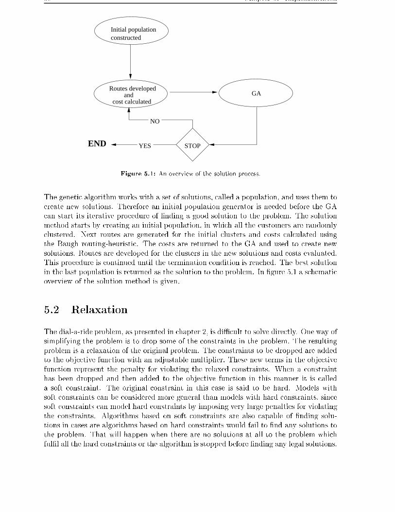
58 Chapter 5. Implementation
Initial populationconstructed
NO
YESEND
GAcost calculated
and Routes developed
STOP
Figure 5.1: An overview of the solution process.
The genetic algorithm works with a set of solutions, called a population, and uses them tocreate new solutions. Therefore an initial population generator is needed before the GAcan start its iterative procedure of �nding a good solution to the problem. The solutionmethod starts by creating an initial population, in which all the customers are randomlyclustered. Next routes are generated for the initial clusters and costs calculated usingthe Baugh routing-heuristic. The costs are returned to the GA and used to create newsolutions. Routes are developed for the clusters in the new solutions and costs evaluated.This procedure is continued until the termination condition is reached. The best solutionin the last population is returned as the solution to the problem. In �gure 5.1 a schematicoverview of the solution method is given.
5.2 Relaxation
The dial-a-ride problem, as presented in chapter 2, is di�cult to solve directly. One way ofsimplifying the problem is to drop some of the constraints in the problem. The resultingproblem is a relaxation of the original problem. The constraints to be dropped are addedto the objective function with an adjustable multiplier. These new terms in the objectivefunction represent the penalty for violating the relaxed constraints. When a constrainthas been dropped and then added to the objective function in this manner it is calleda soft constraint. The original constraint in this case is said to be hard. Models withsoft constraints can be considered more general than models with hard constraints, sincesoft constraints can model hard constraints by imposing very large penalties for violatingthe constraints. Algorithms based on soft constraints are also capable of �nding solu-tions in cases are algorithms based on hard constraints would fail to �nd any solutions tothe problem. That will happen when there are no solutions at all to the problem whichful�l all the hard constraints or the algorithm is stopped before �nding any legal solutions.
5.2 Relaxation 59
The constraints in the dial-a-ride problem can both be represented as hard and soft. Thedecision on whether or not a constraint is allowed to be converted to a soft constraint isbased on an analysis of the underlying problem. The formulated problem in this thesis ispurely theoretical but takes into account practical issues from the Danish transportationoperations. Lets look at the constraints in the problem one at a time.
• Depot constraint must be hard, otherwise each tour will end at the last customersdrop o� location. That is not practical since there is a bus driver in each vehicle whodemands to start and end his tour at one of the depots. It is either not desirable toleave the vehicle unattended somewhere in the city.
• Routing constraint is also kept as a hard constraint, because it is necessary to visitall the pickup and drop o� locations of the customers, since it is not allowed toreject customers in the formulated problem.
• The maximum route duration constraint is, on the other hand, converted to a softconstraint. The upper limit on the route duration in this project represents thelength of the workday of the drivers and it is possible that the drivers can work alittle longer if needed. One could imagine that overtime pay or compensation bydays o� at another time are a part of the job description of the drivers.
• The constraint on maximum customer ride times is also converted to a soft con-straint. The upper limit on maximum ride times is a constant for each customer.The reason for relaxing this constraint is simply making implementation easier. Italso suits the transportation operator, which usually sets this upper limit.
• It is not possible to relax the precedence constraint, since it can produce infeasiblesolutions. That is, it is physically impossible to drop a customer o� before the cus-tomer is picked up.
• The time windows constraints can be relaxed. The advantage of converting hardtime windows to soft time windows is that in practice time windows are usually soft,in the sense that there is a limit up to which a service provider will adhere to thetime windows. The soft time windows are also useful in evaluating the tradeo�s be-tween service requirements and cost requirements. Solutions with soft time windowsindicate the degree of violation allowing penalty methods to distinguish between agiven pair of infeasible solutions in attempting to �nd a feasible region. The timewindows are constructed based on the desired pickup or drop o� time given by thecustomer. The time windows constraints will be converted to soft constraints, i.e.it is allowed to adhere to the desired time given by the customer at an additional cost.
• The capacity constraints can be relaxed if desired. That is however problematic ifthe capacity of all the vehicles �xed and there are no means of adding an extracustomer to the vehicles. The capacity constraint is therefore set to be hard.
For the constraints it has been decided to relax, i.e. time windows, customer ride times,and route duration constraints, penalty factors are added to the objective function along
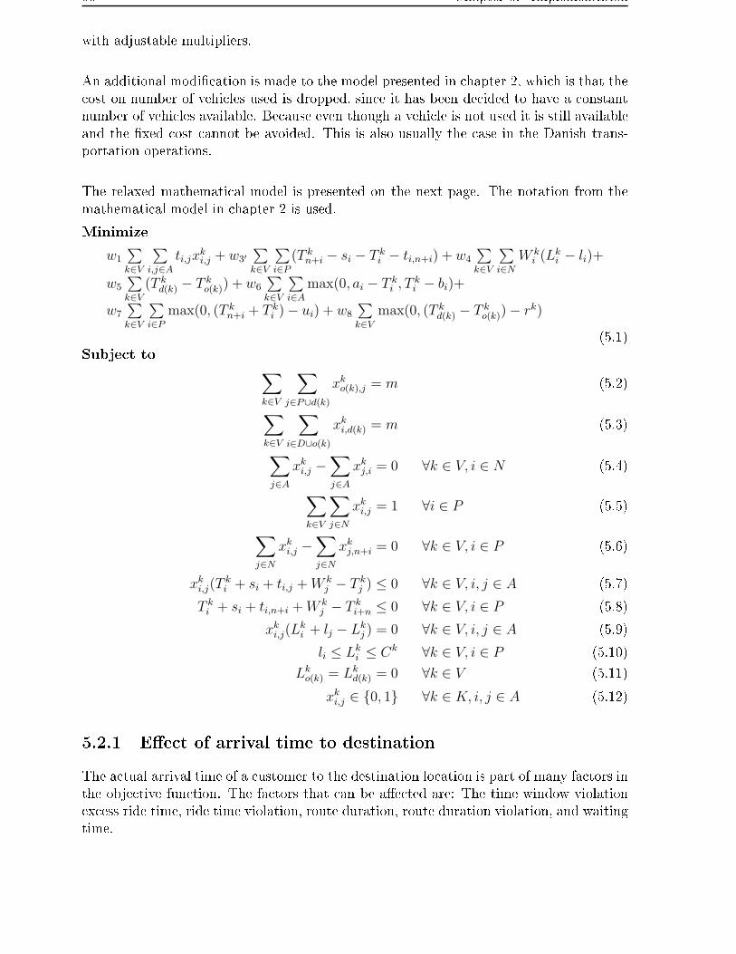
60 Chapter 5. Implementation
with adjustable multipliers.
An additional modi�cation is made to the model presented in chapter 2, which is that thecost on number of vehicles used is dropped, since it has been decided to have a constantnumber of vehicles available. Because even though a vehicle is not used it is still availableand the �xed cost cannot be avoided. This is also usually the case in the Danish trans-portation operations.
The relaxed mathematical model is presented on the next page. The notation from themathematical model in chapter 2 is used.
Minimize
w1
∑k∈V
∑i,j∈A
ti,jxki,j + w3′
∑k∈V
∑i∈P
(T kn+i − si − T k
i − ti,n+i) + w4
∑k∈V
∑i∈N
W ki (Lk
i − li)+
w5
∑k∈V
(T kd(k) − T k
o(k)) + w6
∑k∈V
∑i∈A
max(0, ai − T ki , T k
i − bi)+
w7
∑k∈V
∑i∈P
max(0, (T kn+i + T k
i )− ui) + w8
∑k∈V
max(0, (T kd(k) − T k
o(k))− rk)
(5.1)Subject to ∑
k∈V
∑j∈P∪d(k)
xko(k),j = m (5.2)
∑k∈V
∑i∈D∪o(k)
xki,d(k) = m (5.3)
∑j∈A
xki,j −
∑j∈A
xkj,i = 0 ∀k ∈ V, i ∈ N (5.4)
∑k∈V
∑j∈N
xki,j = 1 ∀i ∈ P (5.5)
∑j∈N
xki,j −
∑j∈N
xkj,n+i = 0 ∀k ∈ V, i ∈ P (5.6)
xki,j(T
ki + si + ti,j + W k
j − T kj ) ≤ 0 ∀k ∈ V, i, j ∈ A (5.7)
T ki + si + ti,n+i + W k
j − T ki+n ≤ 0 ∀k ∈ V, i ∈ P (5.8)
xki,j(L
ki + lj − Lk
j ) = 0 ∀k ∈ V, i, j ∈ A (5.9)
li ≤ Lki ≤ Ck ∀k ∈ V, i ∈ P (5.10)
Lko(k) = Lk
d(k) = 0 ∀k ∈ V (5.11)
xki,j ∈ {0, 1} ∀k ∈ K, i, j ∈ A (5.12)
5.2.1 E�ect of arrival time to destination
The actual arrival time of a customer to the destination location is part of many factors inthe objective function. The factors that can be a�ected are: The time window violationexcess ride time, ride time violation, route duration, route duration violation, and waitingtime.

5.3 The initial heuristic GA1 61
Time
Cos
t
direct transport time upper time window maximum ride time
α=0α=w
3‘
α=w3‘
+w6
α= w3‘
+w6+w
7
Figure 5.2: The in�uence of the arrival time on cost. The slope (α) of the cost increases in stepsdepending on the arrival time.
If the customer arrives on time to his destination within the time windows, the costcontributed by that customers arrival is, if any, the excess ride time. On the other hand,if he is late the time that passes from the upper bound of the time window to actualarrival is both the excess ride time and punishment for every minute the arrival timeexceeds the upper time limit. If the ride time of the customer also exceeds the maximumride time a penalty for that is also added to both the cost of excess ride time and timewindow violation. Above we are assuming that the maximum ride time for the customerplus the pickup time is higher than the upper bound on the drop o� time window. Thiscase is presented in �gure 5.2. So the cost of delivering a customer late increases in stepsdepending on these three constraints and how late the customer is delivered.
If the vehicle arrives too early to a location it has to wait. Two cases can arise; nocustomers are present in the vehicle, or one or more customer sits in the vehicle. In the�rst case the minutes the vehicle has to wait adds a penalty to the cost for violatingthe time windows, the route duration increases and possibly a route duration violationoccurs, if the maximum route duration is exceeded. The reason for having a penalty fora time window violation even though the vehicle is empty is to have the implementationof the time window violation uniformed. If there are customers present in the vehiclethe waiting minutes will add to the cost in several ways: A punishment for time windowviolation adds to cost, the waiting time multiplied by the number of customers present inthe halting vehicle also adds to cost, excess ride time for the customers, route durationincreases and possibly ride time or route duration violations as well.
5.3 The initial heuristic - GA1
In this section the initial heuristic, denoted GA1, used for solving the formulated DARPis described. The section is divided into two main parts which are the same as the twomain parts of GA1, i.e. clustering and routing. In the part about clustering a discussion

62 Chapter 5. Implementation
1 0 1 0 1 0 0 0 1 1 1 0 0 1 0 1 0Route 1
Route 2
Route 4
Route 3
cust
omer
1cu
stom
er 2
cust
omer
3cu
stom
er 4
cust
omer
5cu
stom
er 6
cust
omer
7cu
stom
er 8
depo
t
cust
omer
9cu
stom
er 1
0
cust
omer
11
cust
omer
12
cust
omer
16
cust
omer
15
cust
omer
14
cust
omer
13
1 0 0 0 0 0 0 1 0 0 0 1 0 1 0 0 1
1 0 0 1 0 0 0 0 0 0 0 0 0 0 1 0 0
1 1 0 0 0 1 1 0 0 0 0 0 1 0 0 0 0
Figure 5.3: An example of the binary chromosome representation used in the solution method. Thereare as many columns as customers and depots and as many rows as routes. The number of routes
equals the number of available vehicles. Each customer must be assigned to exactly one route and eachroute has to include the depot.
about the decisions on the structure of the genetic algorithm is presented. In the part onrouting the necessary extensions needed for the Baugh routing-heuristic are presented.
5.3.1 Clustering using GA
The construction of the GA involves taking decisions about which chromosome represen-tation that will best �t the solution to problem, which population size is adequate, howthe initial population should be generated, what stopping criteria to use, how the �tnesscalculations should be made, what kind of selection mechanism is best to use, and whichmodifying operators to use.
Chromosome representation
In order for an individual in the population to represent a solution to the problem ofallocating customers to vehicles it is decided to use a two level binary chromosome rep-resentation. This representation is a binary version of the chromosome representationintroduced by Pereira at al. [13].
In this representation there are as many lines as there are available vehicles and there areas many columns as there are customers and depots. A 1 at any position [g1, g2] indicatesthat the customer/depot represented by column g1 is allocated to the vehicle representedby line g2. In this chromosome representation it is very easy to verify that each customeris allocated to exactly one vehicle. In the formulated dial-a-ride problem there is only onedepot and it is also very easy to verify that all the vehicles routed include the depot. Theveri�cation is performed by adding up all the columns in the chromosome and checkingwhether or not the sum equals the number of vehicles for the �rst column (all the routesinclude the depot) and to 1 for the other columns (each customer is allocated to exactlyone vehicle). A chromosome that ful�lls these constraints, the constraint on each cus-tomer allocation to exactly one vehicle and the depot constraints, is a legal solution to

5.3 The initial heuristic GA1 63
the clustering part of the problem.
In �gure 5.3 there is an example of what the chromosome representation looks like whenthere are four vehicles available, one depot and 16 customers. As we can see each cus-tomer is allocated to exactly one vehicle. The routes can be constructed in many waysfor example route 1 could be constructed in the following way:
depot - 9.1 - 15.1 - 15.2 - 2.1 - 9.2 - 8.1 - 10.1 - 8.2 - 2.2 - 10.2 - 13.1 - 13.2 - 4.1 - 4.2 - depot
where the i.1 is the pickup location of customer i and i.2 is the drop o� location ofcustomer i, for all i in route 1.
Population size
The size of the population greatly in�uences the performance of the GA. If the pop-ulation size is too small it results in a high possibility that the solution space will beunder-covered, while a too large population will be a burden on the computational timeand may lead to unacceptable slow rate of convergence.
In the section about population size for the genetic algorithm (see section 4.2.6) no spe-ci�c guidelines about decisions on the population size are given but instead the di�erent�ndings of some theoretical results are given. Some of which indicate that a populationsize between the length of the string used in the chromosome representation and thedouble length is optimal, while empirical results on the other hand indicate that a popu-lations size as small as 30, independent on the problem size, works well for most problems.
It is decided to use the conventional method of a constant population size and performsome preliminary tests to decide how big the population size has to be for the problemsthat are to be solved. Tests of di�erent sizes of the population will be presented in chapter6.
Initial population
The initial population is created randomly. The consideration kept in mind in the initialpopulation generator is that each customer must be allocated to exactly one vehicle. Thisis easily checked in the chromosome representation by adding up the columns and makesure that this equals exactly one for all the customers. Another consideration is thedepots. In the problem formulation of this project (section 2.6) it is decided to use onlyone depot so the initial solution must have the depot presented in all clusters. That isthe summation of the depot column must equal the number of vehicles available. All theinitial solutions represent therefore a legal solution to the clustering part of the problem.

64 Chapter 5. Implementation
I I I I
R1
R2I2
I1
Req
Figure 5.4: Two resistors in parallel (R1 and R2) have equivalent resistance given by 1Req
= 1R1
+ 1R2
and I is the total current, I1 and I2 are the currents going through resistors R1 and R2 respectively.
Stopping criteria
It is possible to choose from di�erent stopping criteria, such as number of iterations,function of solution quality, the available runtime and no improvements for the last speci�cnumber of iterations. The most common is to use the number of iterations for stoppingcriteria and that will also bee the case in GA1. The main reason for that choice, besidesthe wide spread use of it, is that it is easily implemented, the number of iterations caneasily be altered and are proportional to the runtime. The actual number of iterationsneeded is hard to decide, but in chapter 6 the in�uence on solution quality for threedi�erent number of iterations will be investigated.
Fitness calculations
In the initial algorithm GA1 the �tness of an individual in the population is purely thevalue of the objective function for that particular solution. This is not recommended to[14] but it is easiest to implement and gives possibilities to investigate the e�ect of usingother methods.
The �tness value of a chromosome that represents solution S is:
Φ(S) = vS = fcost(S) + fpenalty(S) (5.13)
where vS is the objective function value for a solution S. fcost(S) represents the four�rst segments in the objective function 5.1 of the relaxed model and fpenalty(S) representsthe total punishment for violating the relaxed constraints, i.e. the last three segmentsof the objective function 5.1 in the relaxed model. For a feasible route, in view of theproblem before relaxation, the fpenalty(S) will equal to zero but for an infeasible route tothe unrelaxed problem the value of fpenalty(S) will be larger than zero, see section 5.2.Even though the problem has been relaxed, at this point it is still desirable to obtainsolutions that ful�ll the relaxed constraints or violate the relaxed constraints as little aspossible. Therefore, in the implementation of the objective function, the segments fpenalty
represents get a large weight, i.e. w6, w7 and w8 are set to high values.
Selection mechanism
In the initial algorithm GA1 two individuals are chosen to produce one o�spring. Oneparent is chosen by means of a stochastic procedure, while the second one is chosen ran-

5.3 The initial heuristic GA1 65
domly. The stochastic procedure also called the roulette wheel method, see section 4.2.10,gives each individual in the current population a probability of being chosen as parentproportional to the �tness value of the individual, i.e. if the individual is in good �tness(represents a low cost solution) the probability of choosing that individual is high, whilethe probability of choosing an individual in bad �tness is low. The only problem encoun-tered using this method is that it is designed for solving a maximization problem, i.e. thehigher �tness value an individual has the more probable it is to chose that particular in-dividual. This is the opposite to solving the dial-a-ride problem, which is a minimizationproblem. We are looking for the cheapest solution and therefore the lowest �tness value.This problem could have been solved by scaling or ranking the objective value in the�tness calculations but it is decided to use the raw objective value in the initial heuristic.The problem is to give solutions with low �tness values high probabilities and vice versaand making sure that the probabilities add up to 1. This problem resembles a problemencountered in electrical physics where the task is to �nd the current through a set ofparallel resistors, see �gure 5.4. First it is necessary to calculate the equivalent resistancefor the parallel resistors, i.e. how big a resistor is needed if the parallel resistors are to bereplaced by a single resistor. Using Ohms law, junction rule and that the resistors havethe same potential di�erence across them, the equivalent resistance is given by:
1
Req
=∑
i
1
Ri
(5.14)
where Ri is the equivalent resistance and Ri is the resistance in resistor i. The currentthrough each resistor is then proportional to the current that enters the parallel connection(indicated by I in �gure 5.4) and the equivalent resistance divided by the current in theresistor, i.e.
Ii = IReq
Ri∀i (5.15)
where Ii is the current through resistance i. Since the same current enters and leaves theparallel resistor the following is true:
1 =∑
i
Req
Ri(5.16)
This can be extended to the problem of constructing a roulette wheel for minimizationproblem. Then the resistance is substituted with the objective function value and the pro-portional current through each resistance (Ii/I) with the probability of using a solution.That is:
1
veq=
∑S
1
vS(5.17)
where vS is the objective value for solution S. The probability of selecting individual Sis then given by:
P (S) =veq
vS
∀S (5.18)
The roulette wheel method in which the selection probabilities are calculated using equa-tion 5.18 is used for selecting parent 1 in GA1.
66 Chapter 5. Implementation
In each iteration one o�spring is created, which replaces one random member that belongsto the Z portion of the current population that have the worst �tness values, i.e. representsolutions with high cost. Z is set to be proportional to the population size and threedi�erent values for Z will be tested in the next chapter. Using this method for updatingthe population, called incremental replacement, the best member of a current populationis guaranteed to survive to the next population. The best solution encountered so far willtherefore never be lost and is allowed to in�uence the development of future generations.
Modifying operators
The main purpose of the crossover operator is to generate better populations as the al-gorithm progresses. The mutation operator helps increasing diversity of the populationand coverage of the solution space. It is necessary to have both mutation and crossoverpresent in the genetic algorithm, otherwise it is impossible to prove the convergence ofthe GA.
The modifying operators in this problem must be capable o� reallocating customers fromone cluster to another, in order for the heuristic to be able to investigate the entire solu-tion space. The modifying operators must also generate legal solutions to the clusteringproblem. In a legal solution to the clustering problem, each customer must be allocatedto exactly one vehicle and the depot must be a part of every route.
• CrossoverThe crossover used in the algorithm is a version of the crossover described by Pereiraet al. [13], which is described in section 4.2.11. In this crossover, one line, i.e. onecluster, is chosen at random from both parents and a random binary template iscreated. The template is used as a recipe for one line in the o�spring, where a 1in the template indicates that the gene is to be taken from parent 2 and the restfrom parent 1. The o�spring consist of the new line while the other lines are dupli-cates from parent 1. When constructing a new solution in this manner it does notnecessarily represent a legal solution. Therefore it is checked if a customer existsthat is assigned to more than one vehicle or no vehicle at all. If such a customer isfound, a cluster is chosen randomly and either the customer is added or deleted fromthat cluster depending on whether the customer is allocated too often or never. Ifthe randomly chosen cluster is the cluster created in the crossover a new cluster israndomly chosen. This procedure is repeated until all the customers are allocatedto exactly one vehicle. It is not necessary to verify that the depot is present in everycluster since the parents represent a legal clustering solution. In each iteration onecrossover is performed resulting in one o�spring.
• Mutation
In the initial heuristic a simple mutation operator is used. The mutation operatormoves one random customer from its current cluster to another random cluster. It isnot possible to generate illegal solutions here using this mutation so no veri�cation orcorrection procedure is needed after mutation. The o�spring that has been createdin the crossover can be subjected to mutation with a certain probability, called the

5.3 The initial heuristic GA1 67
mutation probability, Pµ. It is also possible to apply mutation on other individualsthan the new o�spring. The normal procedure is to apply mutation with a �xedmutation probability to o�springs, which will be performed here as well.
5.3.2 Routing strategy
Latest
timepickup
Lower boundon dropoff TW
boundon dropoff TW
Upper
Time
Service time Direct transport time
Latest possible
departuretime from
locationpickup
si ti,n+i
bn+ian+i
Figure 5.5: Illustration of the latest pickup time calculations for an outbound customer. The latestpickup time is calculated backwards in time. The direct transportation time from pickup to drop oflocation and the service time at the pickup location are subtracted from the upper bound on the drop
o� time window.
Now clusters of customers have been generated using the GA in the �rst phase of thesolution method. In the second phase routes are constructed for the clusters and costsevaluated. The modi�ed space-time nearest neighbour heuristic (Baugh routing-heuristic)described by Baugh et al. is used, in an extended version, for developing routes and cal-culating cost for each route. The Baugh routing-heuristic is described in section 4.3.
In the Baugh routing-heuristic the cost of a route is set to be the weighted sum of traveltime and time window violations. The hard constraints that are included into the heuristicare the routing, precedence and capacity constraints. The depot, maximum route dura-tion and maximum ride time constraints are not included. Neither are excess ride times,waiting times with passengers in the vehicle nor route duration. The missing constraintsand cost factors are added to the heuristic. Service times at each location are also addedto the heuristic.
The method of choosing the �rst customer in a route is also altered. In the Baugh routing-heuristic the �rst customer is chosen to be the customer with the earliest pickup time,which does not give good results for the data used here, since part of the pickup locationshave no time window associated to them. It is the case for outbound customers. Thismeans that the time window is set to the whole planning horizon ([0, T ]) and the lowertime window is zero. Therefore these customers are often chosen as �rst customers, thedrop o� time had no in�uence. In order to account for this, the �rst customer to visitis instead chosen to be the customer with the earliest latest pick up time. For thosecustomers that have no pickup time windows there are assigned latest pickup times based
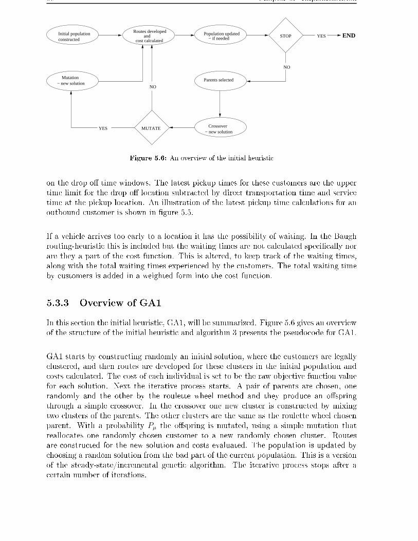
68 Chapter 5. Implementation
Initial populationconstructed cost calculated
and Routes developed
Parents selected
Crossover − new solution
Population updated − if needed
Mutation− new solution
YES ENDSTOP
NO
MUTATEYES
NO
Figure 5.6: An overview of the initial heuristic
on the drop o� time windows. The latest pickup times for these customers are the uppertime limit for the drop o� location subtracted by direct transportation time and servicetime at the pickup location. An illustration of the latest pickup time calculations for anoutbound customer is shown in �gure 5.5.
If a vehicle arrives too early to a location it has the possibility of waiting. In the Baughrouting-heuristic this is included but the waiting times are not calculated speci�cally norare they a part of the cost function. This is altered, to keep track of the waiting times,along with the total waiting times experienced by the customers. The total waiting timeby customers is added in a weighted form into the cost function.
5.3.3 Overview of GA1
In this section the initial heuristic, GA1, will be summarized. Figure 5.6 gives an overviewof the structure of the initial heuristic and algorithm 3 presents the pseudocode for GA1.
GA1 starts by constructing randomly an initial solution, where the customers are legallyclustered, and then routes are developed for these clusters in the initial population andcosts calculated. The cost of each individual is set to be the raw objective function valuefor each solution. Next the iterative process starts. A pair of parents are chosen, onerandomly and the other by the roulette wheel method and they produce an o�springthrough a simple crossover. In the crossover one new cluster is constructed by mixingtwo clusters of the parents. The other clusters are the same as the roulette wheel chosenparent. With a probability Pµ the o�spring is mutated, using a simple mutation thatreallocates one randomly chosen customer to a new randomly chosen cluster. Routesare constructed for the new solution and costs evaluated. The population is updated bychoosing a random solution from the bad part of the current population. This is a versionof the steady-state/incremental genetic algorithm. The iterative process stops after acertain number of iterations.

5.4 Improvements to GA1 69
5.4 Improvements to GA1
The possibilities of improving the initial heuristic are countless. In this section the im-provements that will be tested in the next chapter are described.
Number of o�springs in each iterations set to M - GA2
Some experimental results presented in the literature [14] indicate that it is a better ideato construct generations that are of the same size as the population size, instead of just1 as is the case in GA1. Therefore this will be the �rst e�ort on improving GA1. Whenupdating the population after each iteration the new population will be the best of currentpopulation and the new generation with some random members to increase diversity.
Number of duplicates decreased - GA3
Duplicates distort the selective process and waste computational resources. They aretherefore to be avoided if possible. In GA3 the probability of duplicate chromosomesis reduced by mutating the o�springs that have the same �tness values as their parent1 and therefore represent the same solution. That will produce a di�erent solution tothe problem where one customer has been reallocated. This procedure will not checkwhether or not the solution presented by the mutated o�spring is already present in thepopulation. The reason for that is to save computational time.
Randomness reduced - GA4
In this improvement di�erent methods for reducing the randomness of GA1 is described.
i. Parent 1 always better than parent 2. The parents are chosen in the same manneras in GA1, i.e. parent 1 is chosen using the roulette wheel method and parent 2 ischosen randomly. If this selection results in parent 1 to have a higher �tness valuethan parent 2 the parents are switched. Parent 1 is now parent 2 and parent 2 is nowparent 1. The o�spring always inherits most of its genes from parent 1 and the o�-spring will therefore always inherit more from the better parent in this improvement.
ii. The template not constructed completely randomly. The template used in the crossoverin GA1 is constructed randomly. The template indicates which genes are to be takenfrom which parent. In this improvement the construction of the template is modi-�ed. The probability of taking genes from parent 1 is increased.
iii. Select parent 1 from the best individuals in the population for the last part of the
iterations. For �ne tuning the solution, i.e. �nding a local optimum, the selectionof parent 1 in the last iterations is altered in this improvement. The parent 1 isselected using the roulette wheel method for the �rst iterations as before but in thelast iterations parent 1 is selected randomly among the best individuals (with thelowest �tness values). In the last part of the iterations it is the relative order ofindividuals as that is the basis for selection of parent 1 instead of the raw objective

70 Chapter 5. Implementation
value as is used in the roulette wheel method.
Heuristic run twice while keeping the total number of iterations constant -
GA5
The iterations have been set to a �xed number. It is possible to run the heuristic severaltimes, each time using only part of the iterations, while the total number of iterations iskept constant. A variation of running the heuristic several times without changing thetotal number of iterations is tried in GA5. In GA5 the heuristic is run normally but after acertain number of iterations the current population is mutated (new mutation operator)and the mutated population is used as a new initial solution for running the heuristicagain. The new mutation aims at getting to another part of the solution space. This isperformed by changing all the 0s to 1s and vice versa in the chromosomes. Thereafter thechromosomes are corrected so that they represent legal solutions. After a certain numberof iterations the last populations from each run are combined. The half of the best indi-viduals from each population is used to construct a new population. When selecting thebest individuals from both populations it is necessary to order the individuals and thatis performed using Bubble sort1. The iterations in GA5 are �nished normally using thenewly combined population.
1Bubble sort is a simple way sort an array of objects but not the fastest. The basic idea is to comparetwo neighboring objects, and to swap them if they are in the wrong order. In the �rst iteration all objectsare checked but in each of the following iterations the number of objects checked is reduced by one.

5.4 Improvements to GA1 71
Algorithm 3 GA1' Read data
1: M ← GetPopulationSize
2: G ← GetNumberOfGenerations (iterations)
3: Pµ ← GetMutationProbabilty
4: Z ← GetLevelOfWorstIndividuals
5: car ← GetNumberOfAvailableVehicles
6: stops ← GetNumberOfStops (2×number of customers)
' Initial population constructed
7: P ← RandomPopulationConstructor(M, car, stops)' Routes generated for initial population and costs calculated
8: for (i = 1 : M) do
9: for (j = 1 : car) do10: cluster ← GetCluster(P, i, j)11: route ← MakeRoute(cluster)12: routecost ← GetRouteCost(route)13: end for
14: cost(i) ← ∑j routecost
15: end for
' Genetic algorithm
16: for (i = 1 : G) do
17: random ← GetRandomInteger
' Select Parent 1 using the roulette wheel method
18: for (j = 1 : M) do
19: 1R ←
∑j
1cost(j)
20: end for
21: for (j = 2 : M) do
22: P (j) = P (j − 1) + Rcost(j)
23: end for
24: for (j = 2 : M) do
25: if(P (j − 1) < random < P (j)) Parent1 = j26: end for
' Select Parent 2 randomly
27: Parent2 ← GetRandomInteger
' One o�spring created using crossover
28: Offspring ← Crossover(Parent1, Parent2)'With probability Pµ apply mutation
29: Offspring ← Mutation(Offspring)' Routes for o�spring generated and costs calculated
30: for (j = 1 : car) do31: cluster ← GetCluster(Offspring)32: route ← MakeRoute(cluster)33: routecost ← GetRouteCost(route)34: end for
' Update population, a random solution of the M/Z worst chosen
35: Out ← Select(cost,M/Z)
36: P ← P + Offspring−Out37: cost ← Update
38: end for
39: Return best solution in P
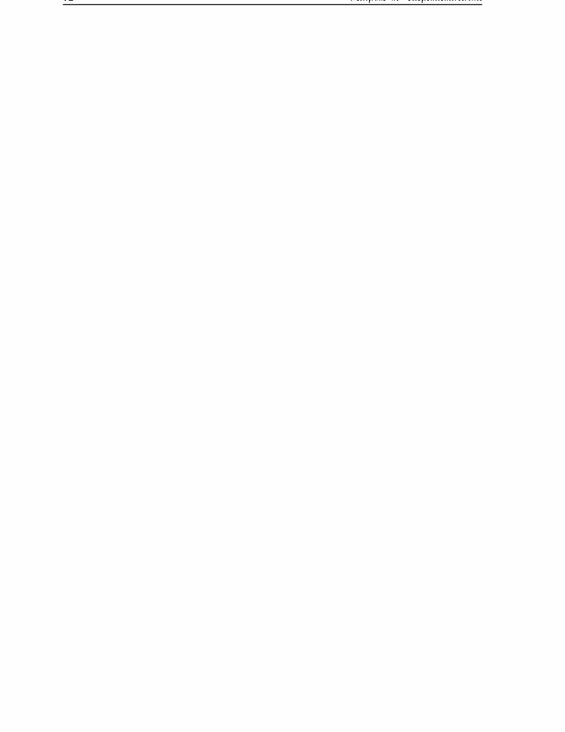
72 Chapter 5. Implementation

Chapter 6
Experimental results
This chapter presents the experimental results obtained from using the chosen solutionapproach for solving the formulated DARP. The solution approach is based on the cluster-�rst, route-second strategy. The genetic algorithm is used in clustering while the Baughrouting-heuristic is used to generate routes for the clusters. The chapter begins by a de-scription of the data that will be used in the experiments. Next the experimental resultswill be presented. The presentation of the experimental results will be divided into thefollowing three main parts.
In the �rst part the main focus will be on testing and tuning the initial heuristic. Firstvalues for four parameters in the genetic algorithm are selected by performing tests onthree data sets and selecting the combination that gives the best results. The parame-ters are population size, number of iterations, mutation probability, and the proportionof the population that can be replaced by a new solution. Secondly, experiments withthe weights in the objective function are performed. It will be shown how they can beadjusted to take into account di�erent points of a view about cost vs. level of service.The customer wants as high service as possible while the transportation operator wantsto provide the minimal accepted service at the lowest cost. The results from these exper-iments and considerations will be used to select values of the weights and the parametersin the GA that will be used in tests performed later in this chapter.
In the second part improvements to the initial heuristic proposed in the last chapter willbe tested. The e�ect of having the generation size equal to the population size, reducingthe number of duplicate solutions present in each population, reducing the randomnessin the heuristic and di�erent iteration approaches will be examined. When each improve-ment has been examined it is either accepted or rejected, that is, either the improvementis used further or eliminated. The later improvements can therefore possibly include pre-vious improvements as well as the improvement itself.
The third part of this chapter is devoted to giving a short comparison of the performanceof the best heuristic obtained in this project and of the simulated annealing solution ap-proach proposed by Cordeau and Laporte [4] for solving the dial-a-ride problem. Theygenerated the random data sets that are used for testing and tuning the initial and im-
73

74 Chapter 6. Experimental results
proved heuristics in this chapter.
6.1 Data
To my knowledge there are no well-known and established benchmarks available in theliterature of the version of DARP used in this project. The behaviour of the solutionmethod proposed here can therefore not be tested using data instances that have beenwidely tested and the results cannot be compared to the optimum or the best resultsobtained previously.
The test instances that will be used for testing the solution method proposed are obtainedfrom Cordeau and Laporte [4]. They created the test instances to analyze the behavior ofthe simulated annealing when solving the DARP. Cordeau and Laporte generated a set of20 randomly generated test instances (data sets) according to realistic assumptions. Theinformation regarding time window widths, vehicle capacity, route duration, and maxi-mum ride time is provided by the Montreal Transit Commission (MTC).
In the test instances there are between 24 and 144 customers. The �rst half of customersis assumed to consists of outbound customers while the remainder of the customers isassumed to be inbound. For each instance, the origin and destination locations are gen-erated using a procedure that creates clusters of vertices around a certain number of seedpoints. All instances contain of a single depot and the location of the depot is set at theaverage location of the seed points. For a more detailed description of this procedure referto Cordeau et al. [3].
For each instance the service time (si) in each location i (i ∈ N) is equal to 10 and theload change, li, in each location i is either 1 or -1. 1 for the pickup locations and -1 forthe drop o� locations, i.e. no customer has a companion travelling with them and all thecustomers need one seat. The depot location on the other hand has a service time andload change equal to zero, since no customers are entering or leaving the vehicle at thedepots. Maximum route duration, rk, in all instances is equal to 480, vehicle capacity,Ck, equal to 6 and maximum ride time, ui, is equal to 90.
A time window [ai, bi] is generated for each location. As mentioned in section 2.5 originpoint of an inbound customer and destination point of an outbound customer are subjectto time windows, while the other points have no customer speci�c time windows associ-ated to them. The time windows for these points is therefore set to [0, T ], where T is theplaning horizon. In the experiments it is equal to 1440, i.e. the number of minutes in oneday - 24× 60 = 1440. The time unit used is minutes.
Two groups of customer speci�c time windows are constructed in the data sets. The �rstone has narrow time windows while the second one has wide time windows. The timewindows in the �rst group are constructed by �rst choosing an uniform random number,

6.1 Data 75
Table 6.1: Size of data instances used in testsCustomers Vehicles
R1a & R1b 24 3R2a & R2b 48 5R3a 72 7R4b 96 9R5a & R5b 120 11R6a & R6b 144 13R07a & R07b 36 4R9a & R9b 108 8R10a & R10b 144 10
ai, in the interval [60, 480] and then choosing another uniform random number, bi, in theinterval [ai + 15, ai + 45]. For the wide time windows group ai is chosen in the samemanner but bi is chosen in the interval [ai +30, ai +90]. Resulting in time windows [ai, bi](i ∈ N). The test instances R1a to R10a have narrow time windows while test instancesR1b to R10b have wide time windows.
Test instances R1a to R6a and R1b to R6b are generated in such a manner that thenumber of available vehicles in comparison to the number of customers is higher than intest instances R7a to R10a and R7b to R10b, e.g. in R6a has 13 available vehicles whileR10a has 10 available vehicles, both instances having 144 customers.
All the test instances constructed by Cordeau and Laporte are available from the Internetat http://www.hec.ca/chairedistributique/data/darp/.
Table 6.1 gives the number of customers and available vehicles in the test instances thatwill be used in this project. Both test instances that have a large and small number ofvehicles available proportional to the number of customers are chosen. In the solutionprocedure used in this report it is not possible to reject customers. The in�uence of the noreject procedure can therefore be investigated. As can be seen, the number of customersis between 24 and 144 and both the instances with narrow and wide time windows arechosen. The reason for not choosing all the data sets given by Cordeau and Laporte isbecause they do not report complete solutions to all the problems. All the problems in ta-ble 6.1 have a given solution except R4b and R7a, which will be used in parameter tuning.
The distance between any two locations i and j is set to be the Euclidean distance be-tween the coordinates of locations i and j, i, j ∈ A. The speed of the vehicles is set to1, so the transportation time ti,j is equal to the Euclidean distance between i and j. Sothe �rst term in the objective function 5.1 equals now the total weighted transportationdistance.

76 Chapter 6. Experimental results
6.2 Testing and tuning the initial heuristic - GA1
In this section the results from solving the DARP using the initial heuristic, GA1, arepresented. GA1 is tested using three di�erent values for four parameters in the geneticalgorithm. The parameters found to give the best results in view of cost are chosen andused for the remainder of the tests performed in this chapter unless otherwise stated.
The solutions obtained by the heuristic vary in di�erent runs of the same data set. It istherefore necessary to perform several runs for each data set. In this project 5 runs foreach solution method on each data set will be performed and the average and best resultsreported. It is desirable to perform a higher number of runs than 5 but that is very timeconsuming and therefore 5 runs are chosen in this project.
6.2.1 Selecting values for the parameters in the GA
The values of four parameters in the genetic algorithm used in clustering the customershave yet to be declared. Those parameters are population size, M , number of generations(iterations), G, mutation probability, Pµ, and the proportion of the current populationthat can be replaced, Z. After performing some initial experiments the following valuesfor the four parameters are chosen to be tested further:
G = {10.000; 15.000; 30.000}M = {30; 50; 100}Pµ = {0, 01; 0, 05; 0, 10}Z = {0, 10; 0, 25; 0, 50}
All 81 combinations of these parameter values are run on three data sets, R4b, R6a, andR7a. These data sets are chosen because they represent both large and small number ofcustomers, narrow and wide time windows and tight and loose constraints on the numberof vehicles compared to number of customers. Furthermore data sets R4b and R7a arealso chosen because Cordeau and Laporte do not give a complete solution to these prob-lems. They can therefore not be used in the comparison of di�erent heuristics later in thechapter anyway.
The choice for the parameter values that are tuned is only based on the cost. Therefore itis the best and average costs obtained from running GA1 for all the combinations of theparameters for the three data sets are presented in tables 6.2, 6.3 and 6.4. The lines in thetables can be divided into three parts, one for each number of iterations (G) tried. Eachof the three parts of lines can again be divided into three parts, one for each populationsize (M) tested. Lastly these three parts can be divided into three lines, one for eachmutation probability (Pµ) tested. Three categories of columns are present in the tables,one for each part of the population that can be termed �bad� (Z).
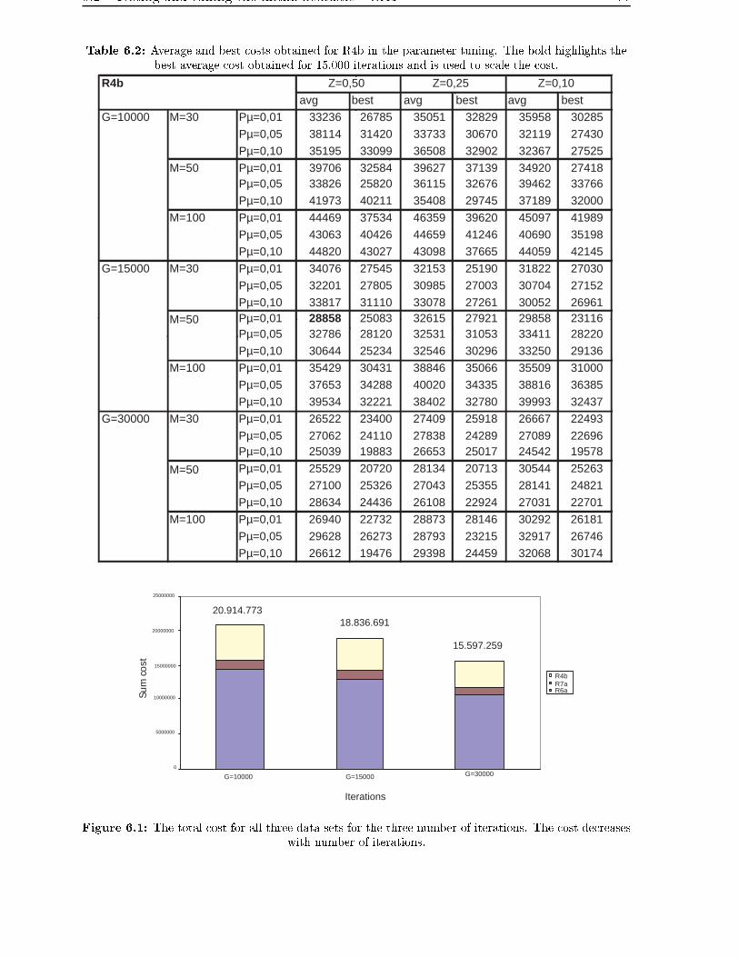
6.2 Testing and tuning the initial heuristic GA1 77
Table 6.2: Average and best costs obtained for R4b in the parameter tuning. The bold highlights thebest average cost obtained for 15.000 iterations and is used to scale the cost.
avg best avg best avg best
Pµ=0,01 33236 26785 35051 32829 35958 30285
Pµ=0,05 38114 31420 33733 30670 32119 27430
Pµ=0,10 35195 33099 36508 32902 32367 27525
Pµ=0,01 39706 32584 39627 37139 34920 27418Pµ=0,05 33826 25820 36115 32676 39462 33766
Pµ=0,10 41973 40211 35408 29745 37189 32000
Pµ=0,01 44469 37534 46359 39620 45097 41989
Pµ=0,05 43063 40426 44659 41246 40690 35198
Pµ=0,10 44820 43027 43098 37665 44059 42145
Pµ=0,01 34076 27545 32153 25190 31822 27030
Pµ=0,05 32201 27805 30985 27003 30704 27152
Pµ=0,10 33817 31110 33078 27261 30052 26961Pµ=0,01 28858 25083 32615 27921 29858 23116Pµ=0,05 32786 28120 32531 31053 33411 28220
Pµ=0,10 30644 25234 32546 30296 33250 29136
Pµ=0,01 35429 30431 38846 35066 35509 31000
Pµ=0,05 37653 34288 40020 34335 38816 36385
Pµ=0,10 39534 32221 38402 32780 39993 32437
Pµ=0,01 26522 23400 27409 25918 26667 22493
Pµ=0,05 27062 24110 27838 24289 27089 22696Pµ=0,10 25039 19883 26653 25017 24542 19578
Pµ=0,01 25529 20720 28134 20713 30544 25263
Pµ=0,05 27100 25326 27043 25355 28141 24821
Pµ=0,10 28634 24436 26108 22924 27031 22701
Pµ=0,01 26940 22732 28873 28146 30292 26181
Pµ=0,05 29628 26273 28793 23215 32917 26746
Pµ=0,10 26612 19476 29398 24459 32068 30174
R4b Z=0,50 Z=0,25 Z=0,10
G=10000
M=100
M=50
M=30
M=100
M=50
G=15000 M=30
G=30000
M=100
M=50
M=30
0
5000000
10000000
15000000
20000000
25000000
G=10000 G=15000 G=30000
R4bR7aR6a
18.836.691
15.597.259
20.914.773
Su
m c
ost
Iterations
Figure 6.1: The total cost for all three data sets for the three number of iterations. The cost decreaseswith number of iterations.
78 Chapter 6. Experimental results
Table 6.3: Average and best costs obtained for R6a in the parameter tuning. The bold highlights thebest average cost obtained for 15.000 iterations and is used to scale the cost.
avg best avg best avg best
Pµ=0,01 94754 86619 86130 80677 88731 76421
Pµ=0,05 95265 77042 96126 88447 98344 92155
Pµ=0,10 96287 91914 89039 72580 92779 83346
Pµ=0,01 102551 89675 102043 84958 98156 87013Pµ=0,05 101775 91209 100271 92151 104844 92408
Pµ=0,10 103225 93660 106121 97621 104782 97257
Pµ=0,01 123050 109879 113652 98036 119761 108304
Pµ=0,05 121809 113784 113990 91064 121300 115203
Pµ=0,10 120890 106611 118530 102408 109100 95476
Pµ=0,01 89123 79594 83945 78462 89357 73131
Pµ=0,05 87086 77743 91769 87825 86882 66397
Pµ=0,10 99905 84919 87491 77448 85391 71198Pµ=0,01 97617 94904 100878 88853 88719 74791Pµ=0,05 95963 91190 91781 83282 88759 77457
Pµ=0,10 98306 85578 91254 80268 89670 81995
Pµ=0,01 101332 79328 102886 94706 103477 91961
Pµ=0,05 106234 100581 105710 103504 100841 95297
Pµ=0,10 96084 86183 113114 104185 107298 92054
Pµ=0,01 80850 77854 70704 66274 74336 63040
Pµ=0,05 85234 76001 75796 64900 76224 66567Pµ=0,10 74222 61250 70174 63718 73249 65153
Pµ=0,01 77591 65891 77815 70128 74957 68186
Pµ=0,05 75899 64319 76668 67720 75976 63897
Pµ=0,10 72265 60873 73377 60912 75427 67690
Pµ=0,01 85162 75922 87715 80421 85181 68275
Pµ=0,05 85081 72969 84251 74251 88205 85478
Pµ=0,10 81092 68230 82603 71086 79743 74837
R6a Z=0,50 Z=0,25 Z=0,10
G=10000
M=50
M=30
M=100
M=100
M=50
M=30G=15000
G=30000
M=100
M=50
M=30
In tables 6.2, 6.3 and 6.4 it can be seen that the cost decreases as the number of iterationsincreases. Figure 6.1 shows that the total cost for all runs of 15.000 iterations is 10%lower than for 10.000 iterations. The total cost for 30.000 iterations is the lowest, or 17%lower than for 15.000 iterations. It seems therefore to be wise to set the number of iter-ations to 30.000 or higher. The drawback is the computational time, which seems to belinearly dependent on the number of iterations. The CPU time for R6a, the largest dataset, is about 150 minutes for 30.000 iterations, 75 minutes for 15.000 iterations and 50minutes for 10.000 iterations. In order to be able to complete the testing of GA1 and theimprovements in a reasonable amount of time as well as obtaining good solutions to theproblem I decided to use 15.000 iterations for further studying and testing. The remarksand conclusions in this chapter are based on the results obtained using 15.000 iterations.
General pattern about the other three parameters is hard to detect. When the problemsize is small a large population results in the lowest average cost, but when the size of

6.2 Testing and tuning the initial heuristic GA1 79
Table 6.4: Average and best costs obtained for R7a in the parameter tuning. The bold highlights thebest average cost obtained for 15.000 iterations and is used to scale the cost.
avg best avg best avg best
Pµ=0,01 9548 8281 8658 7607 9613 8370
Pµ=0,05 8942 8467 10297 8499 8150 7471
Pµ=0,10 9184 7295 8201 6826 8818 6706
Pµ=0,01 8646 7510 8505 7546 9122 8112Pµ=0,05 7916 6511 8035 6487 9433 8270
Pµ=0,10 7513 6244 9003 7445 9192 7447
Pµ=0,01 8762 8002 8941 7191 8762 7229
Pµ=0,05 10600 8940 8667 7989 10020 9182
Pµ=0,10 9660 8614 8518 6993 9114 7707
Pµ=0,01 7810 6859 9004 6623 8702 7065
Pµ=0,05 9194 7211 7985 7537 9268 7542
Pµ=0,10 8765 7921 9319 6883 9155 7064Pµ=0,01 9574 8077 7776 7040 8645 7114Pµ=0,05 8253 7720 8497 6917 8401 7473
Pµ=0,10 8976 7833 9407 7981 8664 6523
Pµ=0,01 8724 7695 8670 6833 7586 6943
Pµ=0,05 7862 7174 8234 7658 8261 7389
Pµ=0,10 8580 5876 8339 7138 8940 7652
Pµ=0,01 8255 7366 8068 7035 6928 6349
Pµ=0,05 7570 6855 8437 7536 8017 6094Pµ=0,10 7256 6413 7845 6382 7717 6398
Pµ=0,01 7361 6621 8005 6780 6978 6230
Pµ=0,05 7951 6594 7977 6900 8361 7736
Pµ=0,10 7860 7029 8158 7404 8403 7462
Pµ=0,01 8109 5820 7512 6840 7418 6385
Pµ=0,05 7888 6525 7455 6667 7689 7424
Pµ=0,10 8015 7067 7837 6172 7632 7316
R7a Z=0,50 Z=0,25 Z=0,10
G=10000
M=100
M=50
M=30
G=15000
M=100
M=50
M=30
M=100
M=50
M=30G=30000
the problem is large it is gives better results to use a small population. One reason forthis behaviour is that the total number of possible di�erent individuals increases withthe number of customers. When the size of the population is large the solution spaceis better covered but it takes a larger number of iterations to reach a local optimum ora near optimum solution. In order to perform a local search in the neighbourhood of agood solution that solution has to be used to produce new solutions in crossover. In thecrossover one parent is chosen randomly and the second parent is chosen proportional tothe �goodness� of the solution. When the number of individuals increases the probabilityof choosing each individual decreases and that goes also for the good solutions. Thereforethe number of times the best individuals are used in crossover is lower than for smallpopulation. For 15.000 iterations M = 30 is best for R6a, M = 50 is best for R4b andM = 100 is best for the smallest data set R7a. That is, the 15.000 iterations are notenough for the larger data sets and as a result the smaller population sizes work betterfor them.

80 Chapter 6. Experimental results
14,5
15
15,5
16
16,5
17
17,5
18
18,5
19
19,5
2 4 10 2 4 10 2 4 10 2 4 10 2 4 10 2 4 10 2 4 10 2 4 10 2 4 10
Pµ=0,01 Pµ=0,05 Pµ =0,01 Pµ=0,01 Pµ=0,05 Pµ =0,10 Pµ=0,01 Pµ=0,05 Pµ =0,10
M=30 M=50 M=100
,
Z -1
Sum
scal
ed c
ost
Figure 6.2: The total scaled cost for all combinations of M , Pµ and Z when G = 15.000 for R4b, R6aand R7a.
The overall best results for the mutation probability is Pµ = 0, 05 closely followed byPµ = 0, 01. For the size of the proportion of the population that can be subject to re-placement Z = 0, 10, i.e. it is possible to choose between M
10individuals to be replaced,
gives the overall best results. These results are obtained by summing the cost from allthe runs for all the combinations of three parameters while keeping Pµ or Z constants.
The data sets have from 36 to 144 customers and the average total cost ranges from 7.586to 123.050. Thus, a raw average will not be a good choice to select the best combinationof the three parameter values. If the raw average would be used then the data sets withhigher cost will have greater weight than the data sets with smaller costs. See for examplein �gure 6.1 that the total cost for R6a is much larger than the total cost for the othertwo smaller data sets. Therefore R6a is a dominant factor in the average total cost for allthe runs. For this reason the costs are scaled by dividing the costs of each combinationin each data set by the minimum average cost for that data set. This minimum averageis indicated by bold in tables 6.2, 6.3 and 6.4. The result of scaling the cost like this isthat the maximum range for the scaled cost in the three data sets is [0,72 ; 1,67] andthe range is similar for all three data sets. Therefore the data sets with higher cost dono longer weigh more than the less expensive ones. A summary of the scaled costs for15.000 iterations is given in �gure 6.2. In the �gure, each column represents the sum ofthe scaled costs of the results for data sets R4b, R6a and R7b for each combination ofthe three remaining parameters. As we can see in the �gure two combinations stand outas the best.
The two best combinations are:
M = 30 Pµ = 0, 05 Z = 0, 25
andM = 50 Pµ = 0, 01 Z = 0, 10
with total scaled costs 16,10 and 16,15 respectively. I decided to use the latter combina-tion since the overall scaled cost for the three data sets is the lowest for population sizeof 50.

6.3 Selecting values for the routing parameters in GA1 81
6.3 Selecting values for the routing parameters in GA1
The routing parameters are the weights, w1 to w8, in the objective function, see sec-tion 5.2. The relative values of these weights in comparison with one another give thecost factors in the objective function di�erent importance levels. The higher the value ofthe weight the more important the cost factor the weight is multiplying becomes. Thesize of the cost factor itself also plays a role in how the weights are to be set. That is,small cost factors need greater weights than larger cost factors in order to have a bearingin how the solutions will develop. The problem of the di�erent sizes of the costs can besolved by scaling the costs before they are entered into the �tness function but that willnot be performed here. Instead the weights will be set to take the di�erent sizes of costfactors into consideration. The weights are:
• w1: weight on driving time, which equals distance here since speed is equal to 1.• w3′: weight on excess passenger ride time.• w4: weight on passenger waiting time.• w5: weight on route duration.• w6: weight on time window violation.• w7: weight on passenger ride time violation.• w8: weight on route time violation.
Note that w2, weight on number of vehicles used, has been omitted from the model sincewe have a constant number of vehicles available, see section 5.2.
In the parameter tuning of the GA in the last section the values for the weights are setto:
w1 = 8, w3′ = 3, w4 = 1, w5 = 1, w6 = 20, w7 = 20, w8 = 20
When selecting the weights no one set of weights represents the �right� set giving the bestresults for some data instances, as is for the parameters in the GA1. The selection ofweights is performed by people and they can represent di�erent points of a view. In thissection two sets of weights will be tested on all the data sets presented in table 6.1 exceptthe three that have been used in the tuning of the GA parameters. One set of weights issupposed to represent customers choice and the second the transportation operator choice.
The results from the �ve runs performed for the 13 data sets used in testing the initial andimproved heuristics are summarized into tables. Each data instance is run 5 times andthe tables present the average results from the data obtained in these runs along with thebest total cost found for each instance. The results tables are made up of eleven columns:
• The �rst column gives the name of the data set for each line.• The second and third columns give the average and best total cost.• The fourth column presents the average passenger cost, i.e. average total cost di-vided by number of customers. The number of customers can be seen in table 6.1.• In the �fth column total distance for the routes in a solution is reported. The routesequal the number of vehicles available and the number of vehicles available in eachdata set can be seen in table 6.1.

82 Chapter 6. Experimental results
• The total route duration is presented in the sixth column.• The seventh column gives the total ride time for the customers.• The eighth column presents the waiting time experienced by the customers.• The ninth column gives the solutions average load of customers in the transportationvehicles. It is calculated based on the following equation 6.1:
Avg load =m∑
p=1
(1
Np
Np∑i=1
Li) (6.1)
where Np is the number of customer stops in route p, Li is the load after servicingat customer stop i and m is the number of vehicles used in the solution.• The tenth column gives the total time window violation for all the stops in theroutes of each data set.• The eleventh column presents the CPU times in minutes. The CPU times aremeasured on an Intel Celeron CPU 2 GHz computer.
The reason for presenting these results for the solutions cost is to being able to investigatethe development of the total cost, which is being minimized in the heuristic. It is alsoimportant to be able to study the route speci�c factors, distance, route duration, ridetime, waiting time, load and time window violation. These factors represent the �real�cost experienced by the customers and/or the transportation operator. Another reason isbeing better able to compare the results for di�erent heuristics.
6.3.1 GA1 - Customers choice
The customers in this section emphasize the level of service provided by the transportationoperator. They want the bus to arrive on time and the ride time to be minimal. On theother hand they do not want the service to be very expensive and therefore they set theirdemands on service to reasonably high levels in their opinion. After performing somepreliminary testing the resulting weights are:
w1 = 8, w3′ = 3, w4 = 1, w5 = 1, w6 = n, w7 = n, w8 = n
The weights on violating the relaxed constraints presented in the objective function (equa-tion 5.1) is set to n, i.e. the total number of customers in each data instance. The reasonfor this choice is that in GA parameter tuning it is experienced that the violation in-creases with the number of customers, because the values for the cost factors for distance,route duration and ride time increase proportionally with the number of customers. Thevalue of the cost terms for the relaxed constraints is not as dependent on the numberof customers as the above mentioned factors. Therefore, it is decided to set the weightsfor the violation terms to n. The weight on total distance driven by the transportationvehicles is set to 8, because the customers are concerned with the transportation cost.The weight on excess ride time is set to 3, as the customers perceive that it is importantthat the transportation time is short. The weights on waiting time with customers is setto 1, because the customers generally do not mind very much waiting in the vehicle aslong as the excess ride time is reasonable. The weight on route duration is also set to1, because the size of the route duration is large compared to the other segments in the

6.3 Selecting values for the routing parameters in GA1 83
�tness function and the customers are not very concerned with the route duration. Thisset of weights is tested on the 13 data sets and the results can be seen in table 6.5.
Table 6.5: GA1 - Weights set by customers choice
Cost Pass. Dist- Route Ride Wait. Avg TW CPU
avg best cost ance durat. time time load viol. [min]
R1a 5162 4729 215 316 1009 568 42 0,99 0 4,41
R2a 20893 14030 435 517 2015 1558 118 1,29 98 10,46
R3a 95377 88571 1325 1050 2844 3529 297 1,56 404 20,03
R5a 266671 237535 2222 1349 4419 5665 552 1,64 1027 55,74
R9a 433888 395670 4017 1379 3676 6267 250 2,01 2282 39,95
R10a 878412 769719 6100 1825 5085 8853 602 2,06 3597 63,41
R1b 4686 4165 195 293 995 540 17 0,94 3 4,41
R2b 17368 11626 362 557 1715 1472 57 1,22 22 10,47
R5b 138511 111773 1154 1353 4214 5377 306 1,64 258 55,82
R6b 262010 219236 1820 1778 5196 6648 397 1,60 522 76,54
R7b 12507 8302 347 485 1270 1169 44 1,24 32 7,03
R9b 252041 224697 2334 1369 3745 5832 319 1,84 932 37,89
R10b 670927 633757 4659 1779 4788 8378 129 2,03 2510 63,27
Total 3058453 2723812 25186 14048 40971 55855 3130 20,06 11687 449,44
We can see in the table that the average passenger cost varies from 215 to 6100 andincreases with number of customers. One reason for this is that the violation weightsare set to n, i.e. to the number of customers, and the violation of these constraintstherefore cost more for the large problems. The probability of getting positive values forthe relaxed segments of the �tness function is also greater for the larger data sets. Bothtotal distance and route duration increases almost linearly with the number of customers.The total passenger ride time is di�erent for the di�erent types of problems present.The ride time is higher when the time windows are narrow and when the vehicles haveincreased average load. The total passenger waiting time in the next column seems togrow with number of customers except for the R10b, which is very low. The average loadsin the vehicles range from 0,94 to 2,06. The top utilization of the transportation vehiclesis achieved when the number of vehicle compared to number of customers is low, as isthe case for R9a, R10a, R7b, R9b and R10b. The CPU times increase with the numberof customers and are higher for data sets with narrow time windows. The CPU timesfor the data sets with fewer number of vehicles per customers is lower than for the datasets with a higher number of vehicles. This is because the routing algorithm used in theheuristic uses about 99% of the CPU time and when the number of vehicles is increasedthe routing algorithm is called more often.
Figures 6.3, 6.4 and 6.5 show how the routes look like for one randomly chosen solutionfor data instance R1a. Figure 6.6 depicts all the three routes together. As we can seethe routes are not localized, meaning that the customers are not divided into groups bylocation. The stronger factor seems to respect the time windows. It can also be seen thatthe customers very often are driven directly from their pickup to their drop o� location(pickup locations have numbers ranging from 1 to 24 and the drop o� locations have the

84 Chapter 6. Experimental results
−6 −5 −4 −3 −2 −1 0 1 2 3−6
−4
−2
0
2
4
6
8Route 1: 0 22 10 46 11 35 7 31 1 34 12 25 2 26 4 36 28 23 47 0
Depot22 [147 177]
10
46
11 35 [178 215]
7 31
1
34
12
25 [258 287]
2
26 [329 361]
4
36 [381 397]
28 [416 460]
23 [471 499]
47
[202 236][260 276]
Figure 6.3: Route 1 for data set R1a (24 customers). The numbers 1 to 24 by a node indicate thepickup location of customers 1 to 24 and numbers 25 to 48 by a node indicate a drop o� location for
customers 1 to 24. The numbers in brackets [] are the time windows for the locations.
same number as the pickup location adding 24 and 0 indicates the depot). The level ofcustomer service is therefore high as the customers want.
−8 −6 −4 −2 0 2 4 6−4
−2
0
2
4
6
8
10Route 2: 0 20 44 3 27 13 37 6 15 39 21 30 45 0
Depot
20 [175 202]
44
3
27 [209 252]
13 [325 358]
37
6 15 [395 421]
39
21 [416 453]
30 [432 458]
45
Figure 6.4: Route 2 for data set R1a (24 customers). The numbers 1 to 24 by a node indicate thepickup location of customers 1 to 24 and numbers 25 to 48 by a node indicate a drop o� location for
customers 25-24 to 48-24. The numbers in brackets [] are the time windows for the locations.

6.3 Selecting values for the routing parameters in GA1 85
−10 −5 0 5−4
−2
0
2
4
6
8
10Route 3: 0 9 17 33 41 14 38 8 32 5 29 24 48 16 40 18 42 19 43 0
Depot
9
17 [86 114]
33 [102 123]
41
14 [111 152]
38
8
32 [225 252]
5 29 [305 349]
24
48
16 [389 401]
40
18 [409 426]
42
19 [454 470]
43 [321 346]
Figure 6.5: Route 3 for data set R1a (24 customers). The numbers 1 to 24 by a node indicate thepickup location of customers 1 to 24 and numbers 25 to 48 by a node indicate a drop o� location for
customers 25-24 to 48-24. The numbers in brackets [] are the time windows for the locations.
−10 −8 −6 −4 −2 0 2 4 6−6
−4
−2
0
2
4
6
8
10All three routes
Depot
Route 1Route 2Route 3
Figure 6.6: All the three routes for R1a together.
6.3.2 GA1 - Operators choice
The transportation operator has di�erent wishes than the customer. The operator wantsto provide minimal service that is still within the service requirements as inexpensively
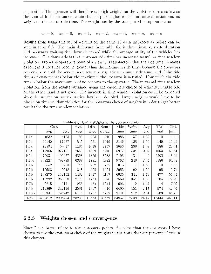
86 Chapter 6. Experimental results
as possible. The operator will therefore set high weights on the violation terms as is alsothe case with the customers choice but he puts higher weight on route duration and noweight on the excess ride time. The weights set by the transportation operator are:
w1 = 8, w3′ = 0, w4 = 1, w5 = 2, w6 = n, w7 = n, w8 = n
Results from using this set of weights on the same 13 data instances as before can beseen in table 6.6. The main di�erence from table 6.5 is that distance, route durationand passenger waiting time have decreased while the average utility of the vehicles hasincreased. The down side is that customer ride time has increased as well as time windowviolation. From the operators point of a view it is satisfactory that the ride time increasesas long as it does not become greater than the maximum ride time, because the operatorsconcern is to hold the service requirements, e.g. the maximum ride time, and if the ridetimes of customers is below the maximum the operator is satis�ed. How much the ridetime is below the maximum is of no concern to the operator. The increased time windowviolation, from the results obtained using the customers choice of weights in table 6.5,on the other hand is not good. The increase in time window violation could be expectedsince the weight on route duration has been doubled. Larger weights would have to beplaced on time window violation for the operators choice of weights in order to get betterresults for the time window violation.
Table 6.6: GA1 - Weights set by operators choice
Cost Pass. Dist- Route Ride Wait. Avg TW CPU
avg best cost ance durat. time time load viol [min]
R1a 4632 4183 193 283 910 986 57 1,52 0 4,44
R2a 26140 17487 545 521 1919 2146 128 1,66 149 10,44
R3a 79594 68017 1105 1018 2757 3683 200 1,69 386 20,31
R5a 317966 277191 2650 1309 4240 6977 504 2,02 1063 56,81
R9a 475031 409457 4398 1326 3588 7103 131 2 2502 43,24
R10a 908227 792889 6307 1781 4922 9762 249 2,34 3586 64,32
R1b 3552 3283 148 252 762 1015 7 1,65 0 4,46
R2b 16683 9648 348 525 1591 2053 92 1,60 95 10,74
R5b 168270 132152 1402 1317 4167 6025 344 1,79 477 56,34
R6b 313292 238888 2176 1734 5096 7569 354 1,83 705 77,28
R7b 9215 6171 256 454 1341 1606 112 1,57 4 7,02
R9b 279869 242116 2591 1307 3610 6490 151 2,17 974 42,94
R10b 880341 794942 6113 1737 4767 9441 212 2,31 3503 64,78
Total 3482812 2996424 28233 13563 39669 64857 2539 24,47 13444 463,11
6.3.3 Weights chosen and convergence
Since I can better relate to the customers points of a view than the operators I havechosen to use the customers choice of the weights in the tests that are presented later inthis chapter.

6.4 Improving the initial heuristic 87
0 5000 10000 150000.6
0.8
1
1.2
1.4
1.6
1.8
2
2.2x 10
5 R5a
Iterations
Cos
t
Figure 6.7: Graphs cost vs. number of iterations for 3 runs for R5a.
Figure 6.7 presents cost vs. number of iterations for three results obtained for R5a. Aswe can see the cost is high in the �rst iterations and then decreases very rapidly in the�rst part of the iterations (around the �rst 2000 iterations). The rate of cost decreasethen diminishes as the number of iterations increases. The results for the three runs aresimilar.
6.4 Improving the initial heuristic
Now all the parameters in GA1 have been determined. It is time to test the improvementstrategies described in chapter 5. First the size of each generation will be changed from1 to M , then the number of duplicates is reduced, next the randomness of GA1 will bereduced and lastly the heuristic will be executed twice in a run. Each improvement istested and either accepted or rejected. When an improvement is accepted it will be apart of later improvements, if rejected it will be eliminated from further testing. Theaim is to �nd the best procedure for solving the formulated DARP. The criteria set foracceptance is that the total average cost decreases and for no more than four individualdata instances the average passenger cost increases. The larger data sets dominate theaverage cost and in order to take better account for the smaller data sets the latter partof the acceptance criteria is set. Even though the selection criterion is purely based onthe cost the results for the routing factors will also be presented. It is interesting to followtheir development as well as the cost and the routing factors will be used later in thechapter for comparing the results obtained by the best procedure to the results obtainedby Cordeau and Laporte [4]. The tables in this section have the same structure as is usedin testing and tuning the initial heuristic, which is described in section 6.3.
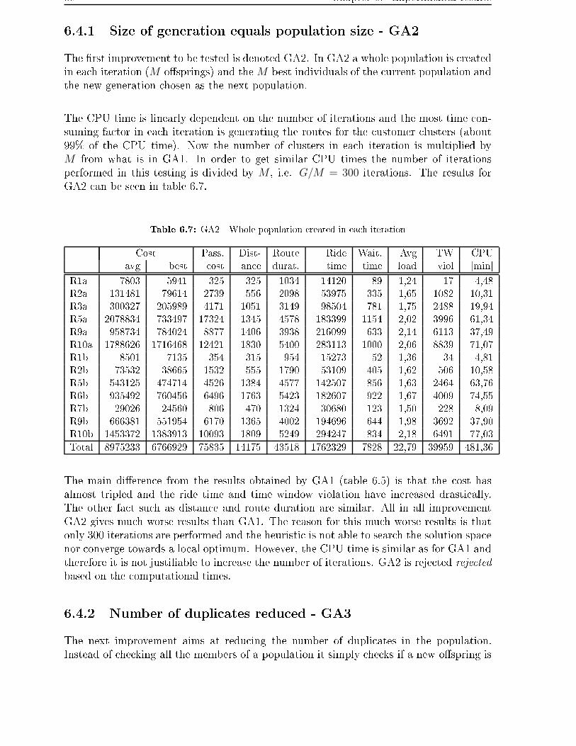
88 Chapter 6. Experimental results
6.4.1 Size of generation equals population size - GA2
The �rst improvement to be tested is denoted GA2. In GA2 a whole population is createdin each iteration (M o�springs) and the M best individuals of the current population andthe new generation chosen as the next population.
The CPU time is linearly dependent on the number of iterations and the most time con-suming factor in each iteration is generating the routes for the customer clusters (about99% of the CPU time). Now the number of clusters in each iteration is multiplied byM from what is in GA1. In order to get similar CPU times the number of iterationsperformed in this testing is divided by M , i.e. G/M = 300 iterations. The results forGA2 can be seen in table 6.7.
Table 6.7: GA2 - Whole population created in each iteration
Cost Pass. Dist- Route Ride Wait. Avg TW CPU
avg best cost ance durat. time time load viol [min]
R1a 7803 5941 325 325 1034 14120 89 1,24 17 4,48
R2a 131481 79614 2739 556 2098 53975 335 1,65 1082 10,31
R3a 300327 205989 4171 1051 3149 98504 781 1,75 2488 19,94
R5a 2078834 733497 17324 1345 4578 183399 1154 2,02 3996 61,34
R9a 958734 784024 8877 1406 3938 216099 633 2,14 6113 37,49
R10a 1788626 1716468 12421 1830 5400 283113 1000 2,06 8839 71,07
R1b 8501 7135 354 315 954 15273 52 1,36 34 4,81
R2b 73532 38665 1532 555 1790 53109 405 1,62 506 10,58
R5b 543125 474714 4526 1384 4577 142507 856 1,63 2464 63,76
R6b 935492 760456 6496 1763 5423 182607 922 1,67 4009 74,55
R7b 29026 24560 806 470 1324 30680 123 1,50 228 8,09
R9b 666381 551954 6170 1365 4002 194696 644 1,98 3692 37,90
R10b 1453372 1383913 10093 1809 5249 294247 834 2,18 6491 77,03
Total 8975233 6766929 75835 14175 43518 1762329 7828 22,79 39959 481,36
The main di�erence from the results obtained by GA1 (table 6.5) is that the cost hasalmost tripled and the ride time and time window violation have increased drastically.The other fact such as distance and route duration are similar. All in all improvementGA2 gives much worse results than GA1. The reason for this much worse results is thatonly 300 iterations are performed and the heuristic is not able to search the solution spacenor converge towards a local optimum. However, the CPU time is similar as for GA1 andtherefore it is not justi�able to increase the number of iterations. GA2 is rejected rejected
based on the computational times.
6.4.2 Number of duplicates reduced - GA3
The next improvement aims at reducing the number of duplicates in the population.Instead of checking all the members of a population it simply checks if a new o�spring is

6.4 Improving the initial heuristic 89
a duplicate of parent 1. If that is the case the o�spring is mutated and thereby a di�erentindividual created. This should increase diversity of the members of the population andlead to a better investigation of the solution space. The results from GA3 can be seen intable 6.8.
Table 6.8: GA3 - Number of duplicates reduced
Cost Pass. Dist- Route Ride Wait. Avg TW CPU
avg best cost ance durat. time time load viol [min]
R1a 4749 4486 198 300 1038 530 30 0,98 1 5,09
R2a 19247 17222 401 529 1971 1675 113 1,38 71 11,54
R3a 74278 65244 1032 1064 2808 3387 248 1,55 248 23,68
R5a 286856 264825 2390 1362 4330 5899 540 1,69 1031 57,36
R9a 405899 363147 3758 1374 3656 6187 172 2,01 2166 39,15
R10a 876352 830424 6086 1794 5055 8940 489 2,10 3587 65,60
R1b 4711 4479 196 306 903 561 4 0,94 2 5,17
R2b 13132 8872 274 551 1651 1368 20 1,21 17 10,94
R5b 131227 112076 1094 1368 4193 5029 281 1,54 224 57,29
R6b 238654 184394 1657 1813 5101 6326 288 1,55 555 78,02
R7b 9081 8074 252 462 1257 1098 67 1,17 4 7,88
R9b 208874 169310 1934 1309 3664 5315 194 1,75 769 39,16
R10b 625965 544459 4347 1734 4813 7972 270 1,98 2271 64,60
Total 2899023 2577013 23619 13964 40441 54285 2715 19,86 10946 465,49
The results for GA3 are compared to the results from GA1 (table 6.5) and it is noticedthat in all areas except vehicle utilization there is an improvement. The average passengercost decreases for all data instances except for R1a and R1b, the smallest instances, wherean increase of 2,5% and 32,4% respectively occurs. The average passenger cost for thelarger data instances decreases up to 28,9% in R10b. The total average cost decreases andan increase in average passenger cost occurs in two data instances, therefore the methodis accepted. Finally it is noticed that by using this method the number of duplicates inthe �nal population is greatly reduced, e.g. for R5a the maximum number of duplicatesfor the last population is 36 using GA1 but 1 using GA3.
6.4.3 Reducing the randomness in the heuristic - GA4
Several parts of the solution process depends on randomness. It is therefore worth whilechecking if reducing the random behavior will improve the results. In this section threemethods of reducing the use of random numbers will be tested. First, parent 1 is setto always represent the better parent, second, the template in the crossover procedure ismodi�ed and third, the selection of parent 1 in the last part of the iterations is limited tothe best individuals in the population.
Parent1 always better than parent 2 - GA4i
In GA4i the parents are chosen in the same manner as in GA1 to GA3. But if parent2 turns out to be the better than parent 1, i.e. has lower cost, the parent numbering

90 Chapter 6. Experimental results
is switched, so that parent 1 always represents a better individual than parent 2. Thismeans that the o�spring always inherits the major part of its genes from the parent withthe better �tness value. The results for GA4i are shown in table 6.9.
Table 6.9: GA4i - Parent1 always better than parent 2
Cost Pass. Dist- Route Ride Wait. Avg TW CPU
avg best cost ance durat. time time load viol [min]
R1a 5037 4605 210 290 1019 580 41 1,00 5 6,21
R2a 19611 13815 409 523 1927 1536 91 1,32 104 11,74
R3a 64481 52726 896 1042 2812 3301 257 1,51 234 21,76
R5a 205320 190686 1711 1374 4353 5399 432 1,60 638 59,14
R9a 333973 286677 3092 1335 3579 5991 178 1,99 1622 40,69
R10a 741004 620435 5146 1784 4955 8380 440 2,02 2845 66,60
R1b 4680 4113 195 294 939 563 0 1,02 2 6,25
R2b 13969 8812 291 530 1627 1325 37 1,18 28 11,81
R5b 126472 103218 1054 1376 4325 4966 262 1,55 214 58,89
R6b 207969 147452 1444 1756 5179 6023 252 1,50 462 80,75
R7b 9204 7499 256 463 1250 1076 21 1,22 7 8,19
R9b 167828 126355 1554 1359 3725 5402 178 1,79 483 40,75
R10b 591027 485320 4104 1803 4885 8102 304 1,99 2061 72,65
Total 2490574 2051715 20361 13930 40574 52644 2493 19,71 8703 485,44
When comparing the results of GA4i with the results of GA3 (table 6.8) we can seethat improvements have occurred in all categories except for route duration which hasslightly increased. The total average cost decreased 14% but in four data instances (R1a,R1b, R2b and R7b) the average passenger cost increases. These four instances are thefour smallest data instances tested and three of them have wider time windows. Thisimprovement therefore lies on the border of being accepted, but it should be noted thatin one (R1a) of the four the increase is almost insigni�cant (0,5%). The improvement,GA4i, is therefore accepted.
Template generated in a less random manner - GA4ii
The next improvement is to modify the template that is used in the crossover procedure.The template is used as a recipe in the crossover, i.e. it indicates which genes are to betaken from which parent. The template is generated in a complete random manner inGA1 to GA4i. In GA4ii the template is created by increasing the probability of selectinggenes from parent 1. It is not wise to increase the probability very much, especially in thebeginning of the iterations, therefore the probability is set to 60%. That is, the probabilityof choosing genes from parent 1 (the better parent) is 60%. The results for GA4ii aregiven in table 6.10.
Comparing the results from the 60% template and the results from GA4ii we can see thatthey are very similar in most categories. The total average cost has though decreased6,4%. The average passenger cost is lower or similar for all data sets except R3a and R5a

6.4 Improving the initial heuristic 91
Table 6.10: GA4ii - Template generated with 60% probability of choosing genes from parent 1
Cost Pass. Dist- Route Ride Wait. Avg TW CPU
avg best cost ance durat. time time load viol [min]
R1a 4696 4193 196 309 1041 477 29 0,89 1 5,57
R2a 19426 14003 405 539 1969 1367 81 1,18 98 11,43
R3a 65306 47801 907 1047 2779 3081 144 1,48 232 21,58
R5a 213420 180109 1778 1350 4250 5099 286 1,57 852 58,23
R9a 333283 299844 3086 1343 3597 6251 132 2,05 1488 40,78
R10a 740890 648300 5145 1811 5006 8413 401 2,00 2989 65,98
R1b 4762 4391 198 284 907 630 5 1,10 0 5,46
R2b 13580 10732 283 561 1719 1214 53 1,07 10 11,72
R5b 98111 74091 818 1344 4296 4615 221 1,45 119 58,93
R6b 185169 156823 1286 1799 5309 6134 361 1,53 384 81,23
R7b 9169 6682 255 478 1299 990 27 1,09 6 8,29
R9b 167709 155366 1553 1372 3679 5362 166 1,77 362 44,66
R10b 474758 419246 3297 1740 4733 7969 202 2,00 1548 66,41
Total 2330280 2021580 19206 13976 40584 51600 2109 19,18 8088 480,28
but in those cases it did not increase much, 1,2% and 3,9% respectively. The results aresatisfactory and the improvement is accepted.
Parent 1 selected from the best individuals for the last iterations - GA4iii
The last e�ort in reducing the randomness of the genetic algorithm is to alter the selec-tion mechanism of parent 1 for the last part of the iterations. Parent 1 is now chosenstochastically using the roulette wheel method. In GA4iii this is altered for the last 1000iterations where parent 1 is chosen randomly among the 15 best individuals in the currentpopulation. The decision on the number of the last iterations is based on that it is desir-able to keep the randomness in the search in the beginning and only �ne tune the solutionat the very end. The decision on 1000 and 15 individuals are results from preliminarytesting performed for the small data instances. The goal of this alteration is to intensifythe search for a local optimum in the last stages of the iterative process. The results forGA4iii are shown in table 6.11.
The results for GA4iii are a little bit worse than the results for GA4ii in table 6.10.The total average cost increases 4,0% and only in �ve data (R2a, R3a, R1b, R2b andR7b) instances the passenger average cost decreases. GA4iii is therefore rejected. Apossible reason for why the improvement does not improve the results is that the decisionson testing this improvement and the exact numbers, used for the last iterations andindividuals to choose parent 1 from, are based on results obtained from the small datainstances. The improvement also seems to work well for the smaller data sets. Theimprovement seems on the other hand not suited for the larger data instances. In thelarger instances the 15.000 iterations are not enough for a thorough investigation of thesolution space and the �ne tuning in the last iterations is waisted. It is better to use themto search for better regions in the solution space. If the number of iterations in GA4iii isincreased, I expect that the results for the larger data sets will also improve.

92 Chapter 6. Experimental results
Table 6.11: GA4iii - Parent 1 chosen from the 15 best for the last 1000 iterations.Cost Pass. Dist- Route Ride Wait. Avg TW CPU
avg best cost ance durat. time time load viol [min]
R1a 4774 4420 199 302 1034 524 28 0,95 1 5,46
R2a 17751 13017 370 524 1935 1487 105 1,22 61 11,40
R3a 63615 46519 884 1047 2821 2928 230 1,39 255 21,45
R5a 216819 181416 1807 1352 4358 5668 443 1,68 617 59,00
R9a 337471 316506 3125 1341 3620 6081 184 2,01 1703 40,19
R10a 711705 645698 4942 1820 5058 8535 376 2,01 2758 67,16
R1b 4522 4059 188 296 895 536 4 0,98 1 5,43
R2b 11356 9136 237 549 1690 1166 28 1,06 6 11,56
R5b 115337 80635 961 1363 4287 4377 192 1,41 213 57,35
R6b 204735 156074 1422 1751 5142 6386 223 1,61 431 79,83
R7b 8867 7728 246 483 1292 1050 36 1,17 3 8,01
R9b 169953 142208 1574 1343 3650 5467 177 6,60 529 40,08
R10b 554837 484938 3853 1781 4880 7843 221 1,95 2014 67,30
Total 2421742 2092355 19808 13953 40663 52048 2246 24,04 8590 474,19
6.4.4 Heuristic run twice and total number of iterations constant
- GA5
The number of iterations is a constant in the testing performed in this chapter, equal to15.000 (except for GA2). When having a constant number of iterations one question thatarises is how to best utilize these iterations. Until now the iterations have been used solv-ing the problem using one initial population. Another possibility is to run the heuristictwice from the start. In the �rst run a part of the total iterations are performed and the�nal population is saved. The �nal population from that run is mutated drastically, inorder to get to another region of the solution space, and the mutated population is usedas an initial population for the second run. In the second run a part of the iterations isperformed and then the �nal population along with the �nal population from the �rst runare combined. In the combination consists of the better half (the M/2 individuals havingthe lowest �tness values) from each �nal population from the two runs. The procedureis �nished running the remainder of the iterations using the combined population as aninitial population. Running the best heuristic encountered so far (GA4ii) in this manneris tested in this section and the improvement is referred to as GA5.
A decision on how many iterations to perform in each run and the last run using thecombined population as an initial solution is needed. In order to make that decisiongraphs of total cost vs. number of iterations are drawn for three randomly chosen runsfrom GA4ii for data sets R1a, R6b and R9a. Those data sets represent all the types ofdata sets that are presented in this chapter. The graphs are shown in �gure 6.8. Whenlooking at the graphs it can be seen that for all the data sets the cost is high in thebeginning and then decreases rapidly and seems to settle, at least for the smallest dataset R1a. The heuristic seems to converge to a local optimum. It can also be seen thatthe rate of decrease in the graphs decreases as the number of iterations increases. Afterabout 5000-6000 iterations the rate of decrease has slowed down and therefore I decided to

6.4 Improving the initial heuristic 93
0 5000 10000 150000.4
0.6
0.8
1
1.2
1.4
1.6
1.8
2
2.2x 10
4 R1a
Iterations
Cos
t
0 5000 10000 150002
3
4
5
6
7
8
9
10
11
12x 10
5 R9a
Iterations
Cos
t
0 5000 10000 150000
2
4
6
8
10
12x 10
5 R6b
Iterations
Cos
t
Figure 6.8: Graphs of cost vs number of iterations. The top �gure is for R1a, the middle one for R9aand the last one for R6b. In each �gure three randomly chosen runs are graphed.
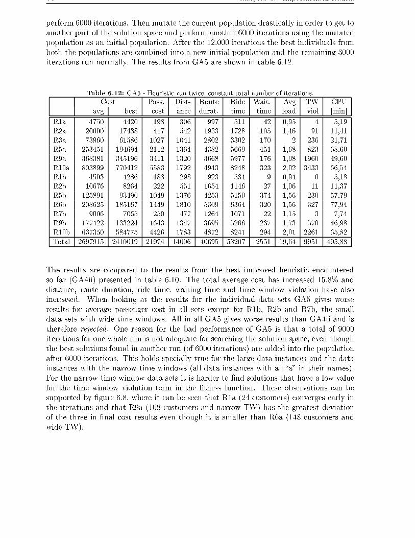
94 Chapter 6. Experimental results
perform 6000 iterations. Then mutate the current population drastically in order to get toanother part of the solution space and perform another 6000 iterations using the mutatedpopulation as an initial population. After the 12.000 iterations the best individuals fromboth the populations are combined into a new initial population and the remaining 3000iterations run normally. The results from GA5 are shown in table 6.12.
Table 6.12: GA5 - Heuristic run twice, constant total number of iterations.
Cost Pass. Dist- Route Ride Wait. Avg TW CPU
avg best cost ance durat. time time load viol [min]
R1a 4750 4420 198 306 997 511 42 0,95 4 5,19
R2a 20000 17438 417 542 1933 1728 105 1,46 91 11,41
R3a 73960 61586 1027 1041 2802 3302 170 2 236 21,71
R5a 253451 194694 2112 1364 4382 5669 451 1,68 823 68,60
R9a 368381 345196 3411 1320 3668 5977 176 1,98 1960 49,60
R10a 803899 770412 5583 1792 4943 8248 323 2,02 3433 66,54
R1b 4503 4286 188 298 923 534 9 0,94 0 5,18
R2b 10676 8264 222 551 1654 1146 27 1,06 11 11,37
R5b 125891 93490 1049 1376 4253 5150 374 1,56 230 57,79
R6b 208625 185167 1449 1810 5309 6364 320 1,56 327 77,94
R7b 9006 7065 250 477 1264 1071 22 1,15 3 7,74
R9b 177422 133224 1643 1347 3695 5266 237 1,73 570 46,98
R10b 637350 584775 4426 1783 4872 8241 294 2,01 2261 65,82
Total 2697915 2410019 21974 14006 40695 53207 2551 19,64 9951 495,88
The results are compared to the results from the best improved heuristic encounteredso far (GA4ii) presented in table 6.10. The total average cost has increased 15,8% anddistance, route duration, ride time, waiting time and time window violation have alsoincreased. When looking at the results for the individual data sets GA5 gives worseresults for average passenger cost in all sets except for R1b, R2b and R7b, the smalldata sets with wide time windows. All in all GA5 gives worse results than GA4ii and istherefore rejected. One reason for the bad performance of GA5 is that a total of 9000iterations for one whole run is not adequate for searching the solution space, even thoughthe best solutions found in another run (of 6000 iterations) are added into the populationafter 6000 iterations. This holds specially true for the large data instances and the datainstances with the narrow time windows (all data instances with an �a� in their names).For the narrow time window data sets it is harder to �nd solutions that have a low valuefor the time window violation term in the �tness function. These observations can besupported by �gure 6.8, where it can be seen that R1a (24 customers) converges early inthe iterations and that R9a (108 customers and narrow TW) has the greatest deviationof the three in �nal cost results even though it is smaller than R6a (148 customers andwide TW).

6.5 The best improvement 95
Table 6.13: The average results obtained by the best improved heuristic, GA4ii, and results from thebest solution for each data set.
Route duration Vehicle waiting time Ride time CPU
Average Best Average Best Average Best time
total avg total avg total avg total avg [min]
R1a 1041 1039 252 5,25 260 5,42 477 19,86 310 12,90 5,57
R2a 1969 1994 470 4,90 514 5,36 1367 28,47 1330 27,72 11,43
R3a 2779 2781 292 2,03 301 2,09 3081 42,79 2894 40,20 21,58
R5a 4250 4274 500 2,08 527 2,20 5099 42,49 4837 40,30 58,23
R9a 3597 3526 94 0,44 32 0,15 6251 57,88 6719 62,21 40,78
R10a 5006 5025 315 1,09 246 0,86 8413 58,42 8341 57,92 65,98
R1b 907 928 143 2,98 164 3,42 630 26,24 549 22,89 5,46
R2b 1719 1710 198 2,06 162 1,69 1214 25,30 1300 27,07 11,72
R5b 4296 4336 552 2,30 568 2,37 4615 38,46 4720 39,33 58,93
R6b 5309 5227 630 2,19 513 1,78 6134 42,59 6397 44,42 81,23
R7b 1299 1316 102 1,41 128 1,78 990 27,50 784 21,76 8,29
R9b 3679 3676 147 0,68 177 0,82 5362 49,65 5358 49,61 44,66
R10b 4733 4678 113 0,39 85 0,29 7969 55,34 8119 56,38 66,41
Total 40584 40508 3808 27,81 3678 28,21 51600 514,99 51657 502,72 488,61
6.5 The best improvement
The initial heuristic and six improvements have been tested. The improved heuristic,named GA4ii, gives the best results in the testing. GA4ii decreases average cost of 23,8%from the initial heuristic GA1, using customers choice of weights, while the CPU timehas gone up 6,9%. The reason for the increased CPU time is that in GA4ii duplicateo�springs are mutated (if a duplicate is produced in a crossover it is mutated and therouting algorithm is run twice for the o�spring) and parents are switched if parent 2represents the better parent. Both these changes to GA1 add a constant time to the CPUtime but the number of times is random. The new method of creating the template doesnot add to the computational time.
6.6 Comparison with Cordeau and Laporte results
In this section the results obtained using the best improved heuristic is compared to theresults obtained by Cordeau and Laporte. The average results from the best improvedheuristic (GA4ii) is presented in table 6.13 along with the results for the best solutionobtained for each data set (i.e. the solution with the lowest cost). Those are some ofthe same results as in table 6.10 but additionally vehicle waiting time is reported. Thevehicle waiting time is not reported in earlier tables since it is not a part of the objectiveto minimize the vehicle waiting time but the passengers waiting time, which is reportedin the tables earlier in the chapter. Cordeau and Laporte on the other hand report thiswaiting time and therefore it is included in table 6.13. The best solutions results are notthat di�erent from the average results, route duration and waiting time little lower andride time little higher.

96 Chapter 6. Experimental results
Table 6.14: Results obtained by Cordeau and Laporte.
Route Vehicle wait. time Ride time CPUduration total average total average [min]
R1a 881 211 4,4 1095 45,62 1,90R2a 1985 724 7,54 1977 41,18 8,06R3a 2579 607 4,22 3587 49,82 17,18R5a 3870 833 3,47 6154 51,3 46,24R9a 3155 323 1,5 5622 52,05 50,51R10a 4480 721 2,5 7164 49,75 87,53R1b 965 321 6,68 1042 43,4 1,93R2b 1565 309 3,22 2393 49,86 8,29R5b 3596 606 2,52 6105 50,87 54,33R6b 4072 449 1,56 7347 51,02 73,70R7b 1097 129 1,79 1762 48,94 4,23R9b 3249 487 2,26 5581 51,68 51,28R10b 4041 362 1,26 7072 49,11 92,41Total 35537 6082 42,92 56900 634,6 497,59
Cordeau and Laporte performed 104 to 105 iterations in order to get their best resultswhich are presented in table 6.14. In the testing in this project 15.000 iterations areperformed. The total CPU time is however comparable. Cordeau and Laporte use aPentium 4, 2 GHz computer in their CPU measurements. Recall that the experiments inthis project are performed on an Intel Celeron CPU 2 GHz computer. It can be pointedout again that on the average 99% of the CPU time in this project is by the routingheuristic.
The objective function used by Cordeau and Laporte is:
v(S) = v1(S) + αv2(S) + βv3(S) + γv4(S) + τv5(S) (6.2)
where v(S) is the objective value for solution S, v1(S) denotes the total routing cost of thevehicles, v2(S) denotes total load violation, v3(S) denotes total route duration violation,v4(S) denotes total time window violation and v5(S) denotes total ride time violation. α,β, γ and τ are a self-adjusting weights. The values of these weights changes in the iter-ations and no approximate values are given in the paper. The method used to calculatethe total routing cost is not speci�ed either in the paper. It is therefore impossible tocompare the cost obtained by the two solution methods.
The other results can be compared to some extent. They are; route duration, ride timeand vehicle waiting time. It can be seen that the route duration is higher in GA4ii than inCordeau and Laporte. The other two results, which are related to customer service, ridetime and vehicle waiting time are on the other hand lower in GA4ii than in the resultsobtained by Cordeau and Laporte. One reason for these results is that the weights areset to represent the customers choice in this project so there is an emphasis on customerservice factors.

6.7 Summary 97
6.7 Summary
Table 6.15: Summary of results obtained by the initial heuristic and the improvements. The upperpart presents the absolute results for each heuristic and the lower part presents the results relative to
GA4ii. A value lower than 1 indicates a lower result than in GA4ii and a higher value than 1 indicates ahigher result.
Cost Pass. Dist- Route Ride Wait. Avg TW CPU
avg best cost ance durat. time time load viol [min]
GA1 3058453 2723812 25186 14048 40971 55855 3130 20,06 11687 449,44
GA2 8975233 6766929 75835 14175 43518 1762329 7828 22,79 39959 481,36
GA3 2899023 2577013 23619 13964 40441 54285 2715 19,86 10946 465,49
GA4i 2490574 2051715 20361 13930 40574 52644 2493 19,71 8703 485,44
GA4ii 2330280 2021580 19206 13976 40584 51600 2109 19,18 8088 480,28
GA4iii 2421742 2092355 19808 13953 40663 52048 2246 24,04 8590 474,19
GA5 2697915 2410019 21974 14006 40695 53207 2551 19,64 9951 495,88
GA1 1,31 1,35 1,31 1,01 1,01 1,08 1,48 1,05 1,44 0,94
GA2 3,85 3,35 3,95 1,01 1,07 34,15 3,71 1,19 4,94 1,00
GA3 1,24 1,27 1,23 1,00 1,00 1,05 1,29 1,04 1,35 0,97
GA4i 1,07 1,01 1,06 1,00 1,00 1,02 1,18 1,03 1,08 1,01
GA4ii 1,00 1,00 1,00 1,00 1,00 1,00 1,00 1,00 1,00 1,00
GA4iii 1,04 1,04 1,03 1,00 1,00 1,01 1,06 1,25 1,06 0,99
GA5 1,16 1,19 1,14 1,00 1,00 1,03 1,21 1,02 1,23 1,03
The initial heuristic along with six improvements have been tested and the results reportedin this chapter and summarized in table 6.15. In the upper part of the table presents thetotal columns for each heuristic and the lower part presents the proportion of each heuris-tics results in comparison to GA4ii. A value lower than 1 indicates a lower result thanobtained by GA4ii, i.e. a better result for all columns except average load. A value higherthan 1 indicates a higher result than for GA4ii, i.e. a worse result for all columns exceptaverage load. The distance, passenger cost, route duration, and ride time for six of theseven results introduced earlier are also summarized in �gure 6.9. In the �gure the re-sults for GA2 are omitted, since GA2 gives much worse results for cost than the other ones.
In the table and the �gure it can be seen that GA4ii gives the best results in all casesexcept for average load. The cost, ride time, waiting time and time window violation areall in�uenced by the improvements while the di�erent heuristics give a near constant re-sults for distance and route duration. The largest improvements for GA4ii are decreasingaverage cost of 23,8% and time window violation of 30,8% compared to GA1. In the othercategories the results are similar but the CPU time has gone up 6,7%. The GA4ii provesto be superior to GA1 and is selected as the best solution method found in this project.
Some of the results that are presented in this chapter came as a big surprise to me. Forexample, I had pictured that the result would improve when the size of the populationin the genetic algorithm is increased. This is not the case. The main reason for that isthat for larger populations, a larger number of iterations are needed in order to perform
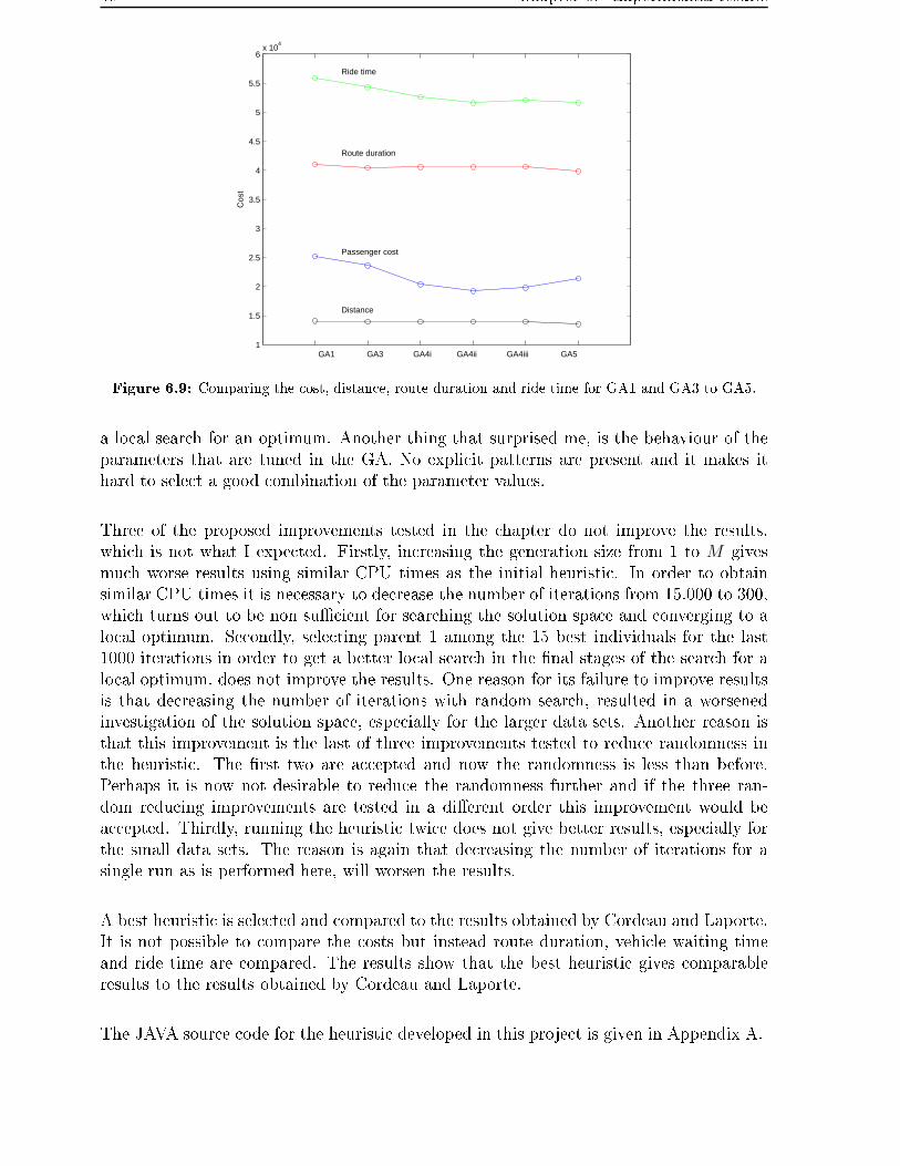
98 Chapter 6. Experimental results
1
1.5
2
2.5
3
3.5
4
4.5
5
5.5
6x 10
4
Passenger cost
Distance
Route duration
Ride time
GA1 GA3 GA4i GA4ii GA4iii GA5
Cos
t
Figure 6.9: Comparing the cost, distance, route duration and ride time for GA1 and GA3 to GA5.
a local search for an optimum. Another thing that surprised me, is the behaviour of theparameters that are tuned in the GA. No explicit patterns are present and it makes ithard to select a good combination of the parameter values.
Three of the proposed improvements tested in the chapter do not improve the results,which is not what I expected. Firstly, increasing the generation size from 1 to M givesmuch worse results using similar CPU times as the initial heuristic. In order to obtainsimilar CPU times it is necessary to decrease the number of iterations from 15.000 to 300,which turns out to be non su�cient for searching the solution space and converging to alocal optimum. Secondly, selecting parent 1 among the 15 best individuals for the last1000 iterations in order to get a better local search in the �nal stages of the search for alocal optimum, does not improve the results. One reason for its failure to improve resultsis that decreasing the number of iterations with random search, resulted in a worsenedinvestigation of the solution space, especially for the larger data sets. Another reason isthat this improvement is the last of three improvements tested to reduce randomness inthe heuristic. The �rst two are accepted and now the randomness is less than before.Perhaps it is now not desirable to reduce the randomness further and if the three ran-dom reducing improvements are tested in a di�erent order this improvement would beaccepted. Thirdly, running the heuristic twice does not give better results, especially forthe small data sets. The reason is again that decreasing the number of iterations for asingle run as is performed here, will worsen the results.
A best heuristic is selected and compared to the results obtained by Cordeau and Laporte.It is not possible to compare the costs but instead route duration, vehicle waiting timeand ride time are compared. The results show that the best heuristic gives comparableresults to the results obtained by Cordeau and Laporte.
The JAVA source code for the heuristic developed in this project is given in Appendix A.
Chapter 7
Conclusion
In this project the focus has been on solving the static dial-a-ride problem using a solutionprocedure not previously used for solving the DARP. Even though the project is mainlytheoretical realistic considerations from a Danish transportation operator have been in-cluded.
The project starts by describing the DARP both in words, by examples and by present-ing the mathematical formulation of DARP. The mathematical formulation is based onexisting literature but a few additions are presented in this project, cost of waiting timewith customers and constraints on maximum route duration and ride time.
An overview of the relevant literature that has given an inspiration to this project is pre-sented. This literature is a part of the background for choosing the method to solve theformulated dial-a-ride problem.
The solution method chosen for solving the DARP is the classical two-phase approachcluster-�rst, route-second. First, customers are clustered and the number of clustersequals the number of available transportation vehicles. Second, a route is developed forall the vehicles. The route is an ordered list of the pickup and drop o� locations ofthe customers along with arrival and departure times at each location. The clustering issolved using the genetic algorithm and the routing is solved using the modi�ed space-timenearest neighbour heuristic developed by Baugh et al. [2]. In the project, the modi�edspace-time nearest neighbour heuristic is extended to include the constraints present inthe formulated DARP. The extensions are to include the hard depot constraints, the softmaximum route duration and maximum ride time constraints. Also included are servicetimes, waiting times with passengers and excess ride times. An initial heuristic is con-structed and six improvements suggested.
The initial heuristic along with the suggested improvements are implemented in JAVA.The initial heuristic is tuned and tested using 16 randomly generated data sets made byCordeau and Laporte [4]. 3 of the 16 data sets are chosen for tuning and the remaining13 for examining the behaviour of the heuristic. Three values for four parameters in the
99
100 Chapter 7. Conclusion
genetic algorithm are selected based on the cost and CPU time results for solutions ob-tained for every combination of the factors. In the initial heuristic it is possible to havedi�erent emphasis on the factors present in the objective function by adjusting the valuesof weights. The results of selecting the weights as a customer and transportation operatorare presented.
A number of potential improvements are tested and de�ne the �nal �product� of thisproject. The results from the �nal �product� heuristic found in this project are comparedto the results given by Cordeau and Laporte. The comparison focuses on route dura-tion, ride and vehicle waiting times. The comparison showed that Cordeau and Laporteobtain better results for route duration whereas th �nal�product� heuristic obtains bet-ter results in the other two categories. The work presented by Cordeau and Laporte canbe considered state-of-the-art within the OR, and my best results are comparable to theirs.
New ideas have been tried in the solution method, which were not encountered in theliterature. One is the method for selecting the �rst customer in a route, which is based onselecting the customer with the earliest latest pickup time. The second is the modi�ca-tion of the roulette wheel method in the genetic algorithm to �t a minimization problem,where ideas are taken from physics.
Several ideas about improvements were left untested due to lack of time. For example touse ranking when selecting parents in the genetic algorithm and to experiment with di�er-ent crossover and mutation operators. I would also have liked to implement a new routingalgorithm. I was not pleased with the modi�ed space-time nearest neighbour heuristic. Itwas described as a fast heuristic but when comparing the CPU times with those obtainedby Cordeau and Laporte that cannot be the case. They are able to perform up to 100.000iterations with the same amount of CPU time as my �best� heuristic in this project useswhen performing 15.000 iterations on almost the same computer. About 99% of the CPUtime of the �best� heuristic is used by the routing algorithm and it would be possible toimprove the performance if a new routing algorithm was implemented. A possible alterna-tive from using the modi�ed space-time nearest neighbour heuristic is to use enumeration,i.e. to check all possible combinations of the stops and select the combination with theleast cost. Another possible alternative is to implement the Lin-Kernighan algorithm [2].
The overall conclusion of this project is that a new solution method that is able to solvethe DARP has been implemented and tested. It is possible to adjust the weights of sevenfactors in the cost calculations. That makes it possible to take di�erent points of a viewof how a dial-a-ride system should look like. The method can therefore be used to exam-ine the in�uence of di�erent strategies and di�erent emphasis in the DAR systems. Thenew solution method has achieved solutions comparable to the current state-of-the-artmethods.
Bibliography
[1] R. Borndorfer, M. Grotschel, F. Klostermeiner and C. Kuttner. Telebus Berlin: Vehi-cle Scheduling in a Dial-a-Ride System. Konrad-Zuse-Zentrum fur Informationstech-nik Berlin, 1997.
[2] J.W. Baugh jr., D.K.R. Kakivaya and J.R. Stone. Intractability of the dial-a-ride
problem and a multiobjective solution using simulated annealing. Engineering Opti-mization, 30(2):91 - 124, 1998.
[3] J.F. Cordeau, M. Gendrau and G. Laporte. A tabu search heuristic for periodic and
multi-depot vehicle routing problems. Networks 30, 105 - 119, 1997
[4] J.F. Cordeau and G. Laporte. A tabu search heuristic for the static multi-vehicle
dial-a-ride problem. Transportation Research, Part B, 37:579 - 594, 2003.
[5] T.H. Cormen, C.E. Leiserson and R.L. Rivest. Introduction to Algorithms. McGraw-Hill Book Company, 2000.
[6] P. Healy and R. Moll. A new extension of local search applied to the dial-a-ride
problem. European Journal of Operational Research, 83(1):83 - 104, 1995.
[7] F. S. Hiller and G. J. Lieberman. Introduction to Operations Research, sixth edition.McDraw-Hill Publishing Company, 1995.
[8] I. Ioachim, J. Desrosiers, Y. Dumas, M. M. Solomon and D. Villeneuve. A re-
quest clustering algorithm for door-to-door handicapped transportation. Transporta-tion Scinece, 29(1):63 - 78, 1995.
[9] J.J. Jaw, A.R. Odoni, H.N. Psaraftis and N.H.M. Wilson. A heuristic algorithm for
the multi-vehicle advance request dial-a-ride problem with time windows. Transporta-tion Research, Part B (Methodological), 20B(3):243 - 257, 1986.
[10] W.R. Jih, C.Y. Kao and F.Y.J. Hsu. Using Family Competition Genetic Algorithm
in Pickup and Delivery Problem with Time Window Constraints. In Proceedings ofthe 2002 IEEE International Symposium on Intelligent Control, Vancouver, Canada,496 - 501, 2002.
[11] R.M. Jørgensen. Dial-a-Ride.Doctor's thesis, Technical University of Denmark, 2002.
101

102 BIBLIOGRAPHY
[12] O.B.G. Madsen, H.F. Ravn and J.M. Rygaard. A heuristic algorithm for a dial-a-
ride problem with time windows, multiple capacities and multiple objectives. Annalsof Operation Research, 60:193 - 208, 1995.
[13] F.B. Pereira, J. Tavares, P. Machado and E. Costa. GVR: a New Genetic Represen-
tation for the Vehicle Routing Problem. Arti�cial Intelligence and Cognitive Science.13th Irish Conference, AICS 2002. Proceedings (Lecture Notes in Arti�cial Intelli-gence Vol. 2464), 95 - 102, 2002.
[14] C.R. Reeves.Modern Heuristic Techniques for Combinatorial Problems.McGraw-HillInternational Limited UK, 151 - 188, 1995.
[15] S.M. Sait and H. Youssef.Iterative Computer Algorithms with Application in Engi-
neering: Solving Combinatiorial Optimization Problems. IEEE Compture Society,109 - 167, 1999.
[16] P. Toth and D. Vigo. Heuristic algorithms for the handicapped persons transportationproblem. Transportation Science, 31(1):60 - 71, 1997.
[17] P. Toth and D. Vigo. Heuristic algorithm for the symmetric and asymmetric vehicle
routing problems with backhauls. European Journal of Operational Research Issue,113(3), 528 - 543, 1999.

Appendix A
JAVA source code
The JAVA source code for the heuristic developed in this project is given as follows:
import java.util.*;
import java.io.*;
class GA5{
public static void main (String[] args) {
long cputime = System.currentTimeMillis();
long routetime=0, rtime;
//Define parameters of the algorithm
String file = "pr16"; //Name of data file
final int M = 50; //Population size
final int G = 15000; //Number of generations, iterations
int Z = (int)M/10; //Worst individuals in population
if (Z==0) Z=1; //At least 1
System.out.println("Z="+Z+" M="+M+" G="+G+" "+file);
final float pm = 1; //Mutation rate * 100
final float big = 3.3E+38f; //big number
float just=60; //likely hood of choosing genes from p1
//float fjust=90; //max likely hood after iterations
//read data file + definations
Request req = new Request(file);
Car vehicle = new Car(file);
int car = vehicle.getNOCar(); //number of cars available
Route26042 ro = new Route26042(file);
final int stops = req.getStops(); //number of stops
//I assume there are always at least 2 stops
//and there is an even number of them
103
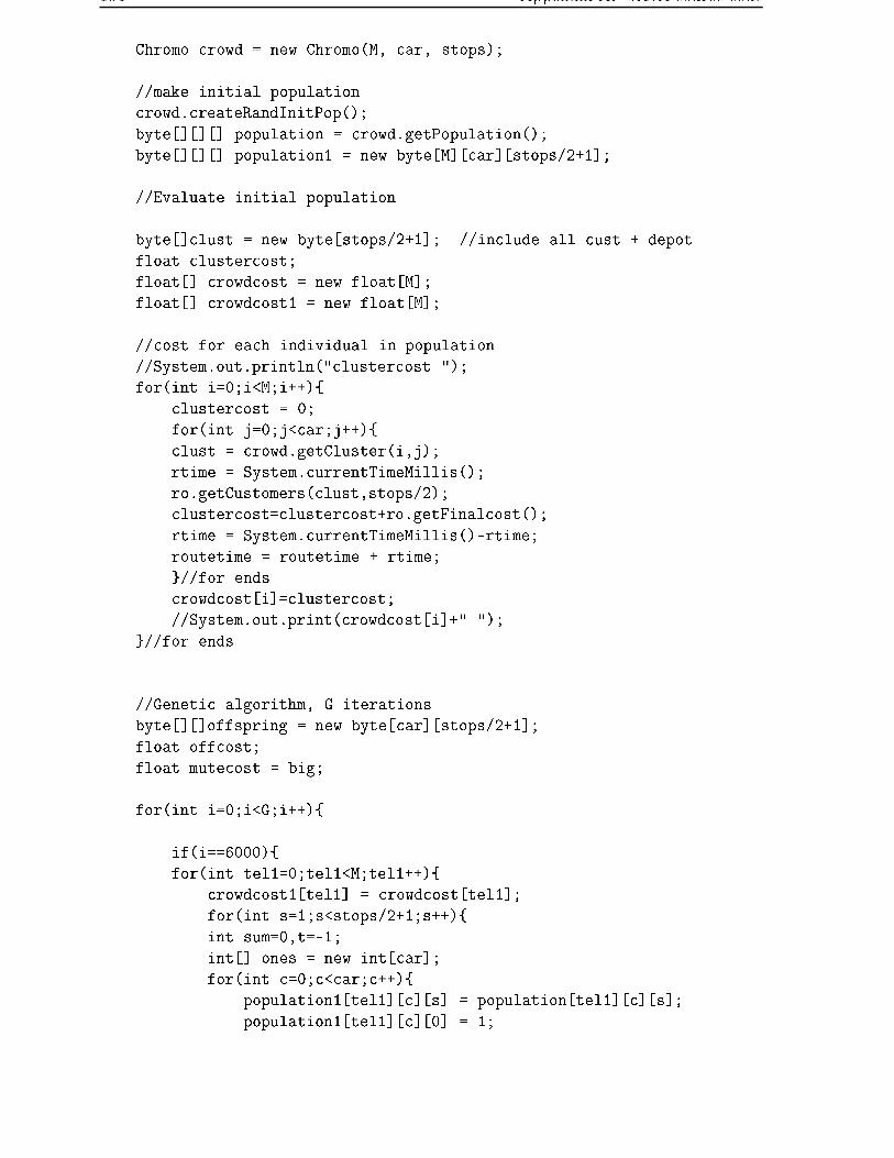
104 Appendix A. JAVA source code
Chromo crowd = new Chromo(M, car, stops);
//make initial population
crowd.createRandInitPop();
byte[][][] population = crowd.getPopulation();
byte[][][] population1 = new byte[M][car][stops/2+1];
//Evaluate initial population
byte[]clust = new byte[stops/2+1]; //include all cust + depot
float clustercost;
float[] crowdcost = new float[M];
float[] crowdcost1 = new float[M];
//cost for each individual in population
//System.out.println("clustercost ");
for(int i=0;i<M;i++){
clustercost = 0;
for(int j=0;j<car;j++){
clust = crowd.getCluster(i,j);
rtime = System.currentTimeMillis();
ro.getCustomers(clust,stops/2);
clustercost=clustercost+ro.getFinalcost();
rtime = System.currentTimeMillis()-rtime;
routetime = routetime + rtime;
}//for ends
crowdcost[i]=clustercost;
//System.out.print(crowdcost[i]+" ");
}//for ends
//Genetic algorithm, G iterations
byte[][]offspring = new byte[car][stops/2+1];
float offcost;
float mutecost = big;
for(int i=0;i<G;i++){
if(i==6000){
for(int tel1=0;tel1<M;tel1++){
crowdcost1[tel1] = crowdcost[tel1];
for(int s=1;s<stops/2+1;s++){
int sum=0,t=-1;
int[] ones = new int[car];
for(int c=0;c<car;c++){
population1[tel1][c][s] = population[tel1][c][s];
population1[tel1][c][0] = 1;

105
if(population[tel1][c][s]==0){
population[tel1][c][s]=1;
t++;
ones[t] = c;
}
else population[tel1][c][s]=0;
sum = sum+population[tel1][c][s];
}//for
if(sum<1) population[tel1][randInt(car)][s]=1;
if(sum>1){
for(int p=1;p<sum;p++){
int rand=randInt(sum);
while (ones[rand]==-1)rand=randInt(sum);
population[tel1][ones[rand]][s]=0;
ones[rand]=-1;
}//for
}//if sum
}//for s
//Evaluate the new mutated population
clustercost = 0;
byte[] line = new byte[stops/2+1];
for(int kk=0;kk<car;kk++){
for(int mm=0;mm<stops/2+1;mm++)
line[mm] = population[tel1][kk][mm];
rtime = System.currentTimeMillis();
ro.getCustomers(line,stops/2);
clustercost=clustercost+ro.getFinalcost();
rtime = System.currentTimeMillis()-rtime;
routetime = rtime+routetime;
}//for ends
crowdcost[tel1]=clustercost;
}//for tel1
printSolution(M,i,crowdcost);
}//end (if i== 6000)
if(i==12000){
Help h = new Help();
float[] cc1=new float[crowdcost1.length];
float[] cc2=new float[crowdcost.length];

106 Appendix A. JAVA source code
for(int ix=0;ix<crowdcost1.length;ix++){
cc1[ix]=crowdcost1[ix];
cc2[ix]=crowdcost[ix];
}
int[]cost1 = h.bubble(cc1);
int[]cost2 = h.bubble(cc2);
for(int t2=M/2;t2<cost2.length;t2++){
int t1 = t2-M/2;
crowdcost[cost2[t2]]=crowdcost1[cost1[t1]];
population[cost2[t2]] = population1[cost1[t1]];
}
}//end if(i==12000)
//select individual stochastically from population
//as parent 1
int rand;
int parent1;
rand = crowd.rand_int(100000000);
parent1 = parenta(M,crowdcost,rand);
//select random individual from population as parent 2
//different than parent 1
int parent2;
do {
parent2 = crowd.rand_int(M);
}while(parent2==parent1);
//if parent2 is better than parent1 then switch
if(crowdcost[parent1]>crowdcost[parent2]){
int parentx;
parentx=parent1;
parent1=parent2;
parent2=parentx;
}
byte[][]p1 = crowd.getIndividual(parent1);
byte[][]p2 = crowd.getIndividual(parent2);
//offspring generated, crossover parent 1 and 2
offspring =
crowd.cross_over2(p1,p2,just);

107
//evaluate offspring
byte[] line = new byte[stops/2+1];
offcost = 0;
for(int kk=0;kk<car;kk++){
for(int mm=0;mm<stops/2+1;mm++)
line[mm] = offspring[kk][mm];
rtime = System.currentTimeMillis();
ro.getCustomers(line,stops/2);
offcost=offcost+ro.getFinalcost();
rtime = System.currentTimeMillis()-rtime;
routetime = rtime+routetime;
}//for ends
//if offsprings cost same as parent 1 then mutate
int key=0;
if(Math.abs(offcost -crowdcost[parent1])< 1E-5f)
key=80;
//Mutation takes place with probability pm
rand = crowd.rand_int(100);
if (rand>=0 && rand<=pm || key==80){
key = 0;
crowd.mutation(offspring);
//evaluate mutated offspring
mutecost = 0;
for(int kk=0;kk<car;kk++){
for(int mm=0;mm<stops/2+1;mm++)
line[mm] = offspring[kk][mm];
rtime = System.currentTimeMillis();
ro.getCustomers(line,stops/2);
mutecost=mutecost+ro.getFinalcost();
rtime = System.currentTimeMillis()-rtime;
routetime = rtime+routetime;
}//for ends
}//if ends
if(mutecost < big) offcost = mutecost;
mutecost = big;
//}//for j ends
//insert offspring for random individual among
//the worst in population
//Z is proportional to M
float[] worst = new float[Z]; //cost of worst individuals
int[] wno = new int[Z];
//indices of corresponding individuals
108 Appendix A. JAVA source code
for(int z=0;z<worst.length;z++){
worst[z] = crowdcost[z];
wno[z] = z;
}//for ends
//small is the index of smallest element in worst
int small = findSmall(worst,M);
for(int t=Z;t<crowdcost.length;t++){
if(worst[small] < crowdcost[t]) {
worst[small] = crowdcost[t];
wno[small] = t;
}
small = findSmall(worst,M);
}//for ends
//choose random individual among the worst with the higest cost
int random = crowd.rand_int(wno.length);
int b = wno[random];
//offspring replaces the chosen individual
//in the current population
crowdcost[b] = offcost;
for(int c=0;c<car;c++){
for(int s=0;s<stops/2+1;s++){
population[b][c][s]=offspring[c][s];
}
}
}//for i ends
cputime = System.currentTimeMillis()-cputime;
//print solution
int small = findSmall(crowdcost,M);
byte[] line = new byte[stops/2+1];
float[]ddist = new float[car];
float[] samtalsridet = new float[car];
float[]rodur = new float[car];
float[]tw = new float[car];
float[]waittime = new float[car];
float[]bidtimifylki = new float[car];
int customer = stops/2;
System.out.print(file+" "+customer);
for(int kk=0;kk<car;kk++){
for(int mm=0;mm<stops/2+1;mm++)

109
line[mm] = population[small][kk][mm];
ro.getCustomers(line,stops/2);
int sum=0;
int[]order = ro.getRoute();
for(int k3=0;k3<order.length;k3++)sum = sum+order[k3];
int ld=0;
int[] load = ro.getLoad();
for(int k6=0;k6<load.length;k6++)ld = ld + load[k6];
int leng = load.length;
float prufa = leng-2;
System.out.print(" sum "+ld);
System.out.print(" "+prufa);
ddist[kk]=ro.getDist();
float[] ride = ro.getRidetime();
for(int je=0;je<ride.length;je++){
if(je%2==1)
samtalsridet[kk]=samtalsridet[kk] + ride[je];
}
float[]time= ro.getTime();
rodur[kk]=ro.getRouteDuration();
float[]window = ro.getTimeWindowsViol();
for(int k7=0; k7<window.length;k7++)tw[kk]=tw[kk]+window[k7];
float summa = 0f;
float[]bidtimi = new float[load.length];
float[]wait = ro.getWaitingTime();
for(int k8=1; k8<wait.length;k8++){
waittime[kk] = waittime[kk] + wait[k8];
bidtimi[k8]=load[k8-1]*wait[k8];
summa = summa + bidtimi[k8];
}
bidtimifylki[kk]=summa;
}//for ends
float samtals=0;
System.out.println("Distance for");
for(int tel=0; tel<ddist.length;tel++){
//System.out.print(" route "+tel+" is "+ddist[tel]);
samtals =samtals+ddist[tel];
}
System.out.println();
System.out.print(" dist "+samtals);
System.out.println();
samtals=0;
System.out.println("Ridetime for passangers in");
for(int tel=0; tel<samtalsridet.length;tel++){
System.out.print(" route "+tel+" is "+samtalsridet[tel]);
samtals =samtals+samtalsridet[tel];

110 Appendix A. JAVA source code
}
System.out.println();
System.out.print(" ride "+samtals);
System.out.println();
samtals=0;
System.out.println("Route duration in");
for(int tel=0; tel<rodur.length;tel++){
System.out.print(" route "+tel+" is "+rodur[tel]);
samtals =samtals+rodur[tel];
}
System.out.print(" route "+samtals);
samtals=0;
System.out.println("Timewindows violation in");
for(int tel=0; tel<tw.length;tel++){
System.out.print(" route "+tel+" is "+tw[tel]);
samtals =samtals+tw[tel];
}
System.out.println();
System.out.print(" tw "+samtals);
samtals=0;
System.out.println("Waiting times in");
for(int tel=0; tel<waittime.length;tel++){
System.out.print(" route "+tel+" is "+waittime[tel]);
samtals =samtals+waittime[tel];
}
System.out.println();
System.out.print(" wait "+samtals);
System.out.println();
samtals=0;
System.out.println("Waiting times in");
for(int tel=0; tel<bidtimifylki.length;tel++){
System.out.print(" route "+tel+" is "+waittime[tel]);
samtals =samtals+bidtimifylki[tel];
}
System.out.println();
System.out.print(" bid "+samtals);
System.out.println();
System.out.print(" M="+M+" G="+G+" pm="+pm+" Z="+Z+" "+file);
System.out.print(" cost "+crowdcost[small]);
System.out.print(" CPU "+cputime);
System.out.println("min: "+cputime/60000);
System.out.print(" Routingrunningtime "+routetime);
System.out.println
("Difference: "+(cputime-routetime)+" or ca "+
((cputime-routetime)*100/cputime)+"%");
System.out.println("Number of customers is "+stops/2);
System.out.println();
111
}//main ends
//print solution
public static void printSolution(int M,int i,float[]crowdcost){
int small = findSmall(crowdcost,M);
System.out.print(i+" , "+crowdcost[small]);
float[]cr = new float[crowdcost.length];
for(int ij=0;ij<cr.length; ij++)
cr[ij]=-crowdcost[ij];
small = findSmall(cr,M);
System.out.println(" , "+crowdcost[small]);
System.out.println();
}
//finds smallest element in an array vec and returns
public static int findSmall(int[] vec, int M){
int small = 2*M, t;
int sm = 2000000000, sm1;
for(t=0;t<vec.length;t++){
sm1=sm;
sm = Math.min(sm,vec[t]);
if(sm != sm1) small = t;
}//for ends
return(small);
}//findSmall ends
public static int findSmall(float[] vec, int M){
int small = 2*M, t;
float sm = 3.0E+38f, sm1;
for(t=0;t<vec.length;t++){
sm1=sm;
sm = Math.min(sm,vec[t]);
if(sm != sm1) small = t;
}//for ends
return(small);
}//findSmall ends
public static int parenta(int M, float[]cost, int rand){
//select individual stochastically from population
//as parent 1
float S=0;
112 Appendix A. JAVA source code
int B=100000000;
for (int index=0;index<M;index++)
S = S + 1/cost[index];
int[] probability = new int[M];
probability[0] = (int)(B/(cost[0]*S));
//probability*B of selecting ind 0 as parent 1
int parent1 = M-1; //default if no patent is chosen,
//because of numeration errors
for(int index=1;index<M;index++){
probability[index] =
probability[index-1] + (int)(B/(cost[index]*S));
}
if(rand < probability[0]) parent1 = 0;
for (int index=1;index<M;index++){
if(rand>=probability[index-1] && rand<probability[index])
parent1 = index;
}//for ends
return(parent1);
} //parenta ends
public static int parentb(int M, float[]cost, int rand){
int small=0;
float[] cro = new float[cost.length];
for(int ij=0;ij<cost.length;ij++)
cro[ij] = cost[ij];
for(int ij=0;ij<=rand;ij++){
small=findSmall(cro,M);
cro[small]=3.3E36f;
}
return(small);
}//parentb ends
public static int randInt(int L){ return((int)(Math.random()*L));}
}//class ends
class Help{
int[] bubble(float[] matrix){
int[] place = new int[matrix.length];
for(int t=0;t<place.length;t++)
place[t] = t;

113
for(int t1=matrix.length-1;t1>0;t1--){
for(int t2=0;t2<t1;t2++){
if(matrix[t2]>matrix[t2+1]){
float temp = matrix[t2];
int tplace = place[t2];
matrix[t2]= matrix[t2+1];
matrix[t2+1]=temp;
place[t2]=place[t2+1];
place[t2+1] = tplace;
}
}
}
return place;
}//bubble ends
}//class ends
class Route26042 {
private int[] v; //customers in cluster
private int[] cs; //customers served
private int[] cv; //customers in vehicle
private int[] cn; //customers not jet served
int MMM; //total number of customers
String filename;
int n; //total number of customers in all clusters
int cun; //number of customers in cluster
int speed = 1; //travelling time equal to E. dist
float w1=1,w2; //(2)weight total route dur and time windows viol
float w3,w4; //weight on ride time and route duration viol
float w5=3,w6=1; //5(0)weight on ex ridetime and waiting time
float w7=8; //weight on distance
int[] ord; //array that holds the order of cust in route
int[] load; //array with number of customers in vehicle after
//a node has been serviced
Request r;
Distance d;
Car car;
float[] ctime, wtime;
public Route26042(String file){filename = file;}
public void giveOrder(int[] order, int nn, float begin){
ctime = new float[order.length];
ctime[0]=begin;

114 Appendix A. JAVA source code
wtime = new float[order.length];
load = new int[order.length];
ord = new int[order.length];
ord = order;
cun = order.length/2-1;
n = nn;
}
public int[] getRoute(){return(ord);}
public float getFinalcost(){
if (ord.length > 2){
float finalcost = ordcost(ord);
return(finalcost);
}
else return(0);
}
public int[] getLoad(){
return(load);
}
public float[] getTime(){
if (ord.length > 2){
float cost = getFinalcost();
}
return(ctime);
}
//returns array with violated times
public float[] getTimeWindowsViol(){
//float cost = getFinalcost();
float[]out = new float[ord.length];
for(int i=0;i<ord.length;i++){
if(ctime[i]>=r.getLTimeWindow(ord[i])+r.getServicetime(ord[i])&&
ctime[i]<=r.getUTimeWindow(ord[i])+r.getServicetime(ord[i]))
out[i]=0;
else if
(ctime[i]<
r.getLTimeWindow(ord[i])+r.getServicetime(ord[i]))
out[i]=
ctime[i]-r.getLTimeWindow(ord[i])-r.getServicetime(ord[i]);
else out[i]=
ctime[i]-r.getUTimeWindow(ord[i])-r.getServicetime(ord[i]);
}//for ends

115
return(out);
}
//returns duration of a route
public float getRouteDuration(){
return(ctime[ctime.length-1]-ctime[0]);
}
//returns ride times of all customers in one route
public float[] getRidetime(){
float[]ride = new float[2*cun];
float cost=ordcost(ord);
int tel=0;
for(int i1=1;i1<ord.length-1;i1++){
if(ord[i1]<=n){
for(int i2=2;i2<ord.length-1;i2++){
if(ord[i2]==ord[i1]+n){
ride[tel] = ord[i1];
ride[tel+1]=ctime[i2]
-ctime[i1]-r.getServicetime(ord[i1]);
tel=tel+2;
}//if
}//for
}//if
}//for
return(ride);
}//getRidetime
//returns waiting times of all nodes in one route
public float[] getWaitingTime(){
return wtime;
}
//returns total distance between nodes in ord
public float getDist(){
float dist=0;
for(int i=0;i<ord.length-1;i++)
dist = dist+d.getDistance(ord[i],ord[i+1]);
return(dist);
}
public void getCustomers(byte[] clu, int MM){
//clu inholds customers to be routed
w2=MM;

116 Appendix A. JAVA source code
w3=MM;
w4=MM;
cun = 0;
for (int kk=1;kk<clu.length;kk++)
cun=cun+clu[kk]; //number of customers in cluster
n = clu.length-1; //total number of customers, depot not included
r = new Request(filename);
d = new Distance(filename);
car = new Car(filename);
//if there are any customers in cluster then continue, otherwise
//return depot to depot route
if(cun > 0){
v = new int[cun];
//v has the number of the customers in the cluster
int count = 0;
for (int i=1;i<clu.length;i++){
if (clu[i]==1){
v[count]=i;
count++;
}//if ends
}//for ends
route();
}//if ends
else {
ord = new int[2];
ord[0] = 0;
ord[1] = 0;
ctime = new float[2];
ctime[0] = 0;
ctime[1] = 0;
}
}//getCustomers ends
// -------------------- ROUTE ------------------------ //
//generate route for a cluster, algorithm taken from Baugh et al
public void route(){
117
ord = new int[2*cun+2]; //order of customers in solution
load = new int[2*cun+2];
ctime = new float[2*cun+2]; //time at which car has
//finished servicing the nodes,
wtime=new float[2*cun+2];
int nnode=-1, cnode=0; //newnode and current node
float ttime=20000, mincost;
//order as in resulting route
int sumcs=0; //sum: cs - customers that have been serviced
int sumcn=0; //sum: cn - customers not in vehicle
int sumv=0; //sum: v - all customers numbers in cluster
int[] firstcust=new int[v.length];
//first customer in route, cust no
int[] firstno=new int[cun];
//number of customer in route
cs = new int[cun];
cv = new int[cun];
cn = new int[cun];
int[]N4 = new int[4]; //4 closest nodes to be considered as next node
//****************************************************
//find cust in v with earliest latest pick-up time
//as first customer in route
int first=-5, no=-5;
float mini=3.3E38f;
float[]ultw = new float[v.length];
for(int re=0;re<v.length;re++){
if(v[re]>n/2) ultw[re]=r.getUTimeWindow(v[re]);
else ultw[re]=r.getUTimeWindow(v[re]+n)-
d.getDistance(v[re],v[re]+n)/speed-
r.getServicetime(v[re]);
if(mini>ultw[re]){mini=ultw[re]; no=re; first=v[re];}
}//for
//values set as -1 to indicate no customer for cs and cv, i.e.
//no customer is in vehicle or has been serviced in the begining,
//all customers number set into cn, customers not serviced
for(int i=0;i<v.length;i++){cn[i]=v[i]; cs[i]=-1; cv[i]=-1;}
118 Appendix A. JAVA source code
cv[no] = first; //first customer added to vehcile
cn[no] = -1; //first customer deleted from cn
ord[0]= 0; //start in depot
ord[1] = first; //then to first customer
load[0] = r.getLoadChange(0);
load[1] = load[0]+r.getLoadChange(first);
//sums calulated, used as stopping criterias in while loop
for(int i=0;i<cs.length;i++){
sumcs = sumcs + cs[i];
sumcn = sumcn + cn[i];
sumv = sumv + v[i];
}
//current node depot, next node first customer,
cnode = 0;
nnode = first;
ttime = d.getDistance(cnode,nnode)/speed;
//travel time from depot to first customer
//find start time for depot, first cust has lowest upper pickup tw
if (first>n/2)
ctime[0]=r.getLTimeWindow(first)-ttime+r.getServicetime(0);
else {
float L = r.getLTimeWindow(first+n)
-d.getDistance(first,first+n)/speed-r.getMaxRideTime();
ctime[0]= L-ttime+r.getServicetime(0);
}
if(ctime[0]<0)ctime[0]=r.getServicetime(0);
ctime[1] = ctime[0] + ttime + r.getServicetime(nnode);
//time after first cust
//if ctime is lower than lower time window, then wait
if(ctime[1] < r.getLTimeWindow(nnode)+r.getServicetime(nnode)){
ctime[1] = r.getLTimeWindow(nnode)+r.getServicetime(nnode);
wtime[1] = ctime[1]-ctime[0]-ttime-r.getServicetime(nnode);
}
//cnode set to first customer
cnode = nnode;
int kkk=1; //counter in while loop, used in ord and ctime
119
//////////////// WHILE LOOP STARTS ///////////////////////
//for(int oj=0; oj<2*cun; oj++){//for perhaps better?
while (sumcn > -cn.length || sumcs<sumv ){
int cek = 0;
for(int i=0;i<N4.length;i++){N4[i]=-1;}
for(int i=0;i<N4.length;i++){
//finds node closest to cnode but not included in N4
if(kkk<ctime.length)
nnode=closest(cnode, ctime, N4,kkk);
else System.out.println("L171 ctime problems");
//nnode=-2 when no more nodes are left
if (nnode==-2 && i==0)
System.out.println("KURT");
if (nnode == -2){
break;
}
else{ //nnode set into N4
int count=0;
for(int j=0;j<N4.length;j++ )
if(N4[j]!=-1)count++;
N4[count] = nnode;
}//else ends
}//for ends
mincost = 3.3E+38f;
//cost of nodes in N4 evaluated and cheapest chosen
for(int i=0;i<N4.length;i++){
if(N4[i] > -1){
if (mincost > cost(N4[i],cnode,ctime,kkk)){
mincost = cost(N4[i],cnode,ctime,kkk);
nnode = N4[i];
}
}
}
//Here something has gone wrong, algorithm should never have
//nnode= -2, it should stop before
if (nnode == -2){

120 Appendix A. JAVA source code
System.out.println("L151 BREAK");
break;
}//end if
kkk++;
visit(nnode);
ttime = d.getDistance(cnode,nnode)/speed;
if (kkk<ctime.length){
ctime[kkk] = ctime[kkk-1] + ttime + r.getServicetime(nnode);
if(ctime[kkk]<r.getLTimeWindow(nnode)+r.getServicetime(nnode)){
ctime[kkk]=r.getLTimeWindow(nnode)+r.getServicetime(nnode);
wtime[kkk]= ctime[kkk]-r.getServicetime(nnode)
-ctime[kkk-1]-ttime;
}
}
cnode = nnode;
load[kkk]=load[kkk-1]+r.getLoadChange(cnode);
//here the while loop has run more times than there are stops ??
if(kkk>ord.length) {
System.out.println("NB!!!! EXTRA LOOP, cnode="+cnode);
cek++;
}
//if ok add cnode into route
if(kkk<ord.length-1 && cnode>0) ord[kkk]=cnode;
else System.out.println("L289 Error in Route "+cnode);
if(cek>0)
System.out.println("Before: sumcs="+sumcs+", sumcn="+sumcn);
//recalculate stopping criterias
sumcs=0;
sumcn=0;
for(int i=0;i<cs.length;i++){
sumcs = sumcs + cs[i];
sumcn = sumcn + cn[i];
}
if(cek>0){
System.out.println("After: sumcs="+sumcs+", sumcn="+sumcn);
System.out.print(" sumv="+sumv+" cn.length="+cn.length);
}
}//while ends
121
}//route ends
// ------------------- CLOSEST ----------------------- //
//Returns node closest to cnode
public int closest(int cnode, float[] ctime, int[] N, int k){
float minldis=3.3E+38f, newldis;
int cstnode = -2, count;
//destination of c not in N
for (int c=0;c<cv.length;c++){
if(cv[c]!= -1){
count = 0;
for (int j=0;j<N.length;j++){
if(N[j]!=cv[c]+n){count++;}
}//for ends
if(count == N.length){
newldis = separation(cnode, cv[c]+n, ctime, k);
if(minldis > newldis){
minldis = newldis;
cstnode = cv[c]+n;
}//if ends
}//if ends
}//if ends
}//for ends
//now it is assumed that the customers travel alone,
//i.e. demand in each node is 1 or -1
count = 0;
for (int c=0;c<cv.length;c++){
if(cv[c]!= -1) count++;
}
if(count == car.getCarCapacity())
return(cstnode);
if(count > car.getCarCapacity()) {
System.out.println("Capacity violated!!!!!!!");
return(cstnode);
}
122 Appendix A. JAVA source code
//origin of c not in N
for (int c=0;c<cn.length;c++){
if(cn[c]!= -1){
count = 0;
for (int j=0;j<N.length;j++){
if(N[j]!=cn[c]){count++;}
}//for ends
if(count == N.length){
newldis = separation(cnode,cn[c] ,ctime,k);
if(minldis > newldis){
minldis = newldis;
cstnode = cn[c];
}//if ends
}//if ends
}//if ends
}//for ends
return(cstnode);
}//closest ends
// ---------------------- SEPARATION -------------------- //
//returns space-time separation between node cnode and nnode
public float separation(int cnode, int nnode,float[] ctime,int k){
float ttime, timek1;
float routedur=0, twviol=0,ridetimeviol=0, exride=0, wt=0;
ttime = d.getDistance(cnode,nnode)/speed;
timek1 = ctime[k] + ttime; //arrival time at nnode
//change in route duration, ctime[k+1]-ctime[k]
routedur = timek1 + r.getServicetime(nnode)-ctime[k];
//tw violations calculated
//for we want to get there soon (twviol>0)
if(timek1>r.getUTimeWindow(nnode))
twviol=timek1-r.getUTimeWindow(nnode);
//tw viol - if early then increase cost - can wait(twviol<0)
if(timek1<r.getLTimeWindow(nnode))
twviol=timek1-r.getLTimeWindow(nnode);
if(timek1 < r.getLTimeWindow(nnode)) //if arrival is to early

123
timek1= r.getLTimeWindow(nnode); //wait until ok
//customers ride time violations caluclated,
//if customer has been in the car for longer than max
//ride time sais then ride time viol > 0, service times of
//customer not included, i.e. nnode is a drop off location
// AND
//customers excess ride times calculated,
//ridetime - direct transport time
if(nnode>n){
for(int i=1;i<ord.length-2;i++){
if(ord[i]==nnode-n){
if(timek1-ctime[i]>r.getMaxRideTime())
ridetimeviol=timek1-ctime[i];
exride=
timek1- ctime[i] - d.getDistance(ord[i],nnode)/speed;
}//if
}//for
}//if
//waiting time calculated * persons in the vehicle
int count = 0;
for (int c=0;c<cv.length;c++){
if(cv[c]!= -1) count++;
}
wt = count*(timek1-(ctime[k] + ttime));
return(w1*routedur-w2*twviol-w3*ridetimeviol
-w5*exride+w6*wt+w7*ttime*speed);
}//separation ends
// ------------------------- COST ------------------------ //
//returns cost of visiting nnode
public float cost(int nnode, int cnode, float[]ctime, int k){
int[]vn = new int[4]; //next four nodes considered
int[]N = new int[4]; //empty array used in call to closest
float totcost = 0;
float ttime; //travel time
124 Appendix A. JAVA source code
int cc = 0;
float ertime; //earliest arrival time to node
for(int i=0;i<4;i++){vn[i]=-1;N[i] = -1;}
for(int i=0;i<4;i++){
totcost = totcost + movecost(cnode, nnode, ctime,k);
if (nnode>0) visit(nnode);
vn[i]=nnode;
ttime = d.getDistance(cnode,nnode)/speed;
ertime = ctime[k] + ttime; //arrival time at nnode
if(ertime<r.getLTimeWindow(nnode))
ertime=r.getLTimeWindow(nnode);
cnode = nnode;
k++;
ctime[k] = ertime + r.getServicetime(cnode);
//service at nnode finished
nnode = closest(cnode,ctime,N,k);
if (nnode==-2) {
cc++;
if (cc==1) {
nnode = 0;
totcost = totcost + movecost(cnode, nnode, ctime,k);
}
else break;
}//end if
}//end for
for(int i=vn.length-1;i>=0;i--){
if(vn[i]> 0)
unvisit(vn[i]);
}//for ends
return(totcost);
}//cost ends
// ----------------------- MOVECOST ------------------- //
//returns cost of move from current node to next node
public float movecost(int cnode, int nnode,float[]ctime, int k){
float ttime, timek1;

125
float routedur=0, twviol=0,ridetimeviol=0, exride=0, wt=0;
ttime = d.getDistance(cnode,nnode)/speed;
timek1 = ctime[k] + ttime; //arrival time at nnode
//change in route duration, ctime[k+1]-ctime[k]
routedur = timek1+wtime[k+1]+r.getServicetime(nnode)-ctime[k];
//tw violations calculated,
if(timek1>r.getUTimeWindow(nnode))
twviol=timek1-r.getUTimeWindow(nnode);
if(ctime[k] + ttime < r.getLTimeWindow(nnode))
twviol=r.getLTimeWindow(nnode)-(ctime[k] + ttime);
if(timek1 < r.getLTimeWindow(nnode)) //if arrival is to early
timek1= r.getLTimeWindow(nnode); //wait until ok
//customers ride time violations caluclated,
//if customer has been in the car for longer than max
//ride time sais then ride time viol > 0, service times of
//customer not included, i.e. nnode is a drop off location
// AND
//customers excess ride times calculated,
//ridetime - direct transport time
if(nnode>n){
for(int i=1;i<ord.length-2;i++){
if(ord[i]==nnode-n){
if(timek1-ctime[i]>r.getMaxRideTime())
ridetimeviol=timek1-ctime[i]-r.getMaxRideTime();
exride=
timek1- ctime[i] - d.getDistance(ord[i],nnode)/speed;
}//if
}//for
}//if
//waiting time calculated * persons in the vehicle
int count = 0;
for (int c=0;c<cv.length;c++){
if(cv[c]!= -1) count++;
}
wt = count*(timek1-(ctime[k] + ttime));
return(w1*routedur + w2*twviol + w3*ridetimeviol
+ w5*exride + w6*wt + w7*ttime*speed);
}//movecost ends

126 Appendix A. JAVA source code
// ----------------------- ORDCOST ------------------- //
//Returns cost of route
public float ordcost(int[] order){
float ttime, routeviol=0, serv, routedur=0,twviol=0;
float rideviol=0,xride=0,wt=0;
int cnode, nnode;
for(int i=0;i<cv.length;i++){cv[i]=-1;cs[i]=-1;cn[i]=v[i];}
load[0]=0;
cnode = order[0];
ctime[0]=retime();
for(int j=0;j<wtime.length;j++)
wtime[j]=0;
//update ctime, wtime, load for the route found
for(int i=1;i<order.length;i++){
nnode = order[i];
load[i]=load[i-1]+r.getLoadChange(order[i]);
ttime = d.getDistance(cnode,nnode)/speed;
ctime[i] = ctime[i-1]+ttime+r.getServicetime(nnode)+wtime[i];
if(ctime[i]<r.getLTimeWindow(nnode)+r.getServicetime(nnode)){
ctime[i]=r.getLTimeWindow(nnode)+r.getServicetime(nnode);
wtime[i]=ctime[i]-(ctime[i-1]+ttime+r.getServicetime(nnode));
}//if ends
if(i>1 && wtime[i]>0 && load[i-1]>load[i-2]) wait(i);
//if(diff>-1) totcost = diff;
cnode = nnode;
if(cnode>0) visit(cnode);
}//for ends
for(int i=1;i<order.length;i++){
ttime = d.getDistance(order[i-1],order[i])/speed;
serv = r.getServicetime(order[i]);
//tw violations calculated,
if(ctime[i]-serv>r.getUTimeWindow(order[i]))
twviol=twviol+(ctime[i]-serv)-r.getUTimeWindow(order[i]);
if(ctime[i-1]+ttime<r.getLTimeWindow(order[i]))
twviol=twviol+r.getLTimeWindow(order[i])-(ctime[i-1]+ttime);
//customers ride time violations caluclated,
//if customer has been in the car for longer than max

127
//ride time sais then ride time viol > 0, service times of
//customer not included, i.e. nnode is a drop off location
// AND
//customers excess ride times calculated,
//ridetime - direct transport time
if(order[i]>n){
for(int j=1;j<order.length-2;j++){
if(order[j]==order[i]-n){
if(ctime[i]-serv-ctime[j]>r.getMaxRideTime()){
rideviol= rideviol+ ctime[i]-serv-
ctime[j]-r.getMaxRideTime();
}
xride=xride+ctime[i]-serv-ctime[j]
-d.getDistance(order[i],order[j])/speed;
}//if
}//for
}//if
//waiting time calculated * persons in the vehicle
wt = wt+load[i-1]*(ctime[i]-serv-(ctime[i-1]+ttime));
}
if(wt<1E-5)wt=0;
//total route duration
routedur = ctime[ctime.length-1]-ctime[0];
//route duration violations calculated,
//if current time is higer than
//max allowable route duration then route viol becomes > 0
if(ctime[ctime.length-1]-ctime[0]>car.getRouteDuration())
routeviol =
ctime[ctime.length-1]-ctime[0]-car.getRouteDuration();
return(w1*routedur+w2*twviol+w3*rideviol
+w4*routeviol+w5*xride+w6*wt+w7*getDist());
}//ordcost ends
// ------------------------- RETIME -------------------------//

128 Appendix A. JAVA source code
//Recalculate starting time so that time windows are not violated
public float retime(){
float ttime;
if(ctime[ctime.length-1]>r.getUTimeWindow(ord[ord.length-1]))
ctime[ctime.length-1]=r.getUTimeWindow(ord[ord.length-1]);
for(int i=ctime.length-1;i>0;i--){
ttime = d.getDistance(ord[i],ord[i-1])/speed;
ctime[i-1] = ctime[i]-ttime-r.getServicetime(ord[i]) ;
if(ctime[i-1]<
r.getLTimeWindow(ord[i-1])+r.getServicetime(ord[i-1]))
ctime[i-1]=
r.getLTimeWindow(ord[i-1])+r.getServicetime(ord[i-1]);
if(ctime[i-1]>
r.getUTimeWindow(ord[i-1])+r.getServicetime(ord[i-1]))
ctime[i-1]=
r.getUTimeWindow(ord[i-1])+r.getServicetime(ord[i-1]);
}//for ends
return(ctime[0]);
}
// -------------------------- WAIT -----------------------//
//moves waiting times to nodes where there are fewer customers
//in the vehicle
public void wait(int no){
float start=wtime[no];
float diff=0;
for(int i=no;i>1;i--){
diff=r.getUTimeWindow(ord[i-1])
-ctime[i-1]+r.getServicetime(ord[i-1]);
//arrival time within tw
if(load[i-2]>load[i-1]|| wtime[i]<0.01 || diff<=0)break;
else{
if(diff>0 && diff<=wtime[i]){
wtime[i-1]=wtime[i-1]+diff;
ctime[i-1]=ctime[i-1]+diff;
wtime[i]=wtime[i]-diff;
diff=0;
}

129
if(diff>0 && diff>wtime[i]){
wtime[i-1]=wtime[i-1]+wtime[i];
ctime[i-1]=ctime[i-1]+wtime[i];
wtime[i]=0;
}
}//else ends
}//for ends
}//wait ends
// -------------------------- VISIT -------------------- //
//marks gnode as visited by updating global data
public void visit(int gnode){
for(int c=0;c<v.length;c++){
if(gnode==v[c]){
cn[c] = -1;
cv[c] = v[c];
break;
}
if(gnode==v[c]+n){
cs[c] = v[c];
cv[c] = -1;
break;
}
}//for ends
}//visit ends
// -------------------------- UNVISIT -------------------- //
//marks gnode as not visited by updating global data
public void unvisit(int gnode){
for(int c=v.length-1;c>=0;c--){
if(gnode==v[c]){

130 Appendix A. JAVA source code
cn[c] = v[c];
cv[c] = -1;
break;
}
if(gnode==v[c]+n){
cs[c] = -1;
cv[c] = v[c];
break;
}
}//for ends
}//uvisit ends
}//class ends
class Request {
int [][] req;
float [][] coo;
Data s;
int st, max;
public Request(){}
//Constructer that initializes matrices and reads in values
public Request(String filename){
final int sizereq=4, sizecoo=2;
Data s = new Data(filename);
st = s.getStops();
req = new int[st][sizereq];
coo = new float[st][sizecoo];
coo = s.getCoo();
req = s.getReq();
max = s.getMaxRideTime();
}//Request constructer ends
public int getStops(){return(st);}
public int getMaxRideTime(){return(max);}
public float[][] getCooMatrix(){
return(coo);
}//getCooMatrix ends
public float getxCoordinates(int custnum){
float x= coo[custnum][0];
return(x);

131
}//getxCoordinates ends
public float getyCoordinates(int custnum){
float y= coo[custnum][1];
return(y);
}//getyCoordinates ends
public float[] getxy(int custnum){
float[] xy = new float[2];
xy[0] = getxCoordinates(custnum);
xy[1] = getyCoordinates(custnum);
return(xy);
}
public int getServicetime(int custnum){
int s=req[custnum][0];
return(s);
}//getServicetime ends
public int getLoadChange(int custnum){
int c=req[custnum][1];
return(c);
}//getLoadChange ends
public int getLTimeWindow(int custnum){
int tw = req[custnum][2];
return(tw);
}//getlTimeWindow ends
public int getUTimeWindow(int custnum){
int tu = req[custnum][3];
return(tu);
}//getuTimeWindow ends
}//Request class ends
public class Data{
private LineNumberReader in;
int[] prob = new int[5];
float[][]coo;
int[][]req;
static int count;
String filename;
//method that reads number of depots, number of stops, max duration
//time of a tour, max capacity of cars, max riding time of customers
public Data(String file){
filename = file; readProblem(); read();

132 Appendix A. JAVA source code
}
public void readProblem() {
try{
in = new LineNumberReader(new FileReader(filename));
StringTokenizer dimen;
//reads the information into a vector prob
for (int i=1; i<2;i++){
String dimension = in.readLine();
dimen = new StringTokenizer(dimension);
while(dimen.hasMoreTokens()){
prob[0] = Integer.parseInt(dimen.nextToken());
prob[1] = Integer.parseInt(dimen.nextToken());
prob[2] = Integer.parseInt(dimen.nextToken());
prob[3] = Integer.parseInt(dimen.nextToken());
prob[4] = Integer.parseInt(dimen.nextToken());
}//while ends
}//for ends
}//try ends
catch (EOFException eof) {
closeFile();
}
catch (IOException e){
System.out.println("1 The file "+filename+" could not be opened "
+e.toString());
System.exit (1);
}//CATCH ENDS
}//readProblem ends
//method that returnes number of vechicles available
int getNOCar(){
return(prob[0]);
}
//method that returnes number of stops
int getStops(){
return(prob[1]);
}
//method that returns allowable route duration
int getRouteDuration(){
return(prob[2]);
}
//method that returns capacity of cars
int getCapacity(){
return(prob[3]);

133
}
//method that returns maximum riding time for customers
int getMaxRideTime(){
return(prob[4]);
}
//method that reads cooridnates of customers into a matrix coo and
//service time, load change, lower time window and upper time window
//into matrix req
public void read(){
try{
in = new LineNumberReader(new FileReader(filename));
StringTokenizer tokens;
//Reads cooridinates of the customers into a matrix coo
//and rest into a matrix req
int dim = getStops()+1;
int car = getNOCar();
req = new int[dim][4];
coo = new float[dim][2];
int d=0;
if(dim-1>0 && dim-1<10) d = 0;
if(dim-1>9 && dim-1<100) d = 1;
if(dim-1>99 && dim-1<1000) d = 2;
if(car>9 && car<100) d = d +1;
in.skip(12+d);
for(int i=0; i< dim+1;i++){
String tokenstring = in.readLine();
int index;
tokens = new StringTokenizer(tokenstring);
while(tokens.hasMoreTokens()){
index = Integer.parseInt(tokens.nextToken());
coo[index][0] = Float.parseFloat(tokens.nextToken());
coo[index][1]
= Float.parseFloat(tokens.nextToken());
req[index][0]
= Integer.parseInt(tokens.nextToken());
req[index][1]
= Integer.parseInt(tokens.nextToken());
req[index][2]
= Integer.parseInt(tokens.nextToken());
req[index][3]

134 Appendix A. JAVA source code
= Integer.parseInt(tokens.nextToken());
}//WHILE ENDS
} //FOR ENDS
} //TRY ENDS
catch (EOFException eof) {
closeFile();
}
catch (IOException e){
System.out.println("2 The file "+filename+" could not be opened "
+e.toString());
}//CATCH ENDS
}//readRequest ends
private void closeFile() {
try{
in.close();
System.exit(0);
}
catch (IOException e) {
System.err.println("Error closing file" + e.toString());
System.exit (1);
}
}//closeFile ends
public float[][] getCoo(){return(coo);}
public int[][] getReq(){return(req);}
} //CLASS Data ENDS
class Distance{
protected float [][] dist;
int sto;
float[][]dcoo;
public Distance(String filename){
Request r = new Request(filename);
sto = r.getStops();
dist = new float[sto+1][sto+1];
dcoo=r.getCooMatrix();
calculateDistance();
}//Distance Constructur ends
public void calculateDistance(){
for(int s=0;s<sto+1;s++){dist[s][s]=0;}
for(int s1=0;s1<sto+1;s1++){
for(int s2=0;s2<s1;s2++){
dist[s1][s2] =

135
(float)Math.sqrt((dcoo[s1][0]-dcoo[s2][0])*
(dcoo[s1][0]-dcoo[s2][0])+
(dcoo[s1][1]-dcoo[s2][1])*
(dcoo[s1][1]-dcoo[s2][1]));
}//for ends
}//for ends
for(int s1=0;s1<sto+1;s1++){
for(int s2=s1+1;s2<sto+1;s2++){
dist[s1][s2]=dist[s2][s1];
}//for ends
}//for ends
}//calculateDistance ends
//returnes distance between stop 1 and 2
public float getDistance(int cust1, int cust2){
return(dist[cust1][cust2]);
}//getDistance ends
}//Distance class ends
class Car {
int capacity, carno;
String filename;
Data d;
public Car(String file){
filename = file;
d = new Data(filename);
}
public int getCarCapacity(){return d.getCapacity();}
public int getNOCar(){return d.getNOCar();}
public int getRouteDuration(){return d.getRouteDuration();}
}//Car class ends
class Chromo extends Request{
byte[][][]ind;
int[][] sum;
int stops, car, pop;
public Chromo(){}
public Chromo(int p, int c, int st){
pop=p; car=c ; stops=st;
}

136 Appendix A. JAVA source code
public void createRandInitPop(){
int rand;
ind = new byte[pop][car][stops/2+1];
for(int i=0;i<pop;i++){
for (int j=0;j<car;j++)
ind[i][j][0]=1;
for(int k=1;k<stops/2+1;k++){
rand=rand_int(car);
ind[i][rand][k]=1;
}//for ends
}//for ends
checkPopulation();
//printMatrix(ind[0]);
//printMatrix(ind[1]);
}//createRandIndPop ends
public byte[][][] getPopulation(){return ind;}
public byte[][] getIndividual(int a){
byte[][]parent = new byte[car][stops/2+1];
for(int i=0;i<car;i++){
for(int j=0;j<stops/2+1;j++){parent[i][j]=ind[a][i][j];}
}
return(parent);
}
public byte[]getCluster(int a, int b){
byte[] clust = new byte[stops/2+1];
for (int i=0;i<stops/2+1;i++){clust[i]=ind[a][b][i];}
return(clust);
}
public void checkPopulation(){
int rand;
for(int i=0;i<pop;i++){
int sum=0;
for(int j=0;j<car;j++)
sum = sum + ind[i][j][0];
if(sum != car)
System.out.println("Error for depot "+sum+" car "+car);
for(int k=1;k<stops/2+1;k++){
int su=0;
for(int j=0;j<car;j++){su=su+ind[i][j][k];}

137
switch(su){
case 0:
rand=rand_int(car);
ind[i][rand][k]=1;
break;
case 1:
break;
default:
System.out.println
("Error individiual "+i+" car "+k);
}//switch ends
}//for ends
}//for ends
}//checkPopulation ends
public void custInCar(){
sum = new int[pop][car];
for(int i=0;i<pop;i++){
for (int j=0;j<car;j++){
for (int k=0;k<stops/2;k++){
sum[i][j]=sum[i][j]+ind[i][j][k];
}//for ends
}//for ends
}//for ends
}//CustInCar ends
public int getCustInCar(int ind,int carno){
custInCar();
return(sum[ind][carno]);
}
//cross over in which there is selected randomly rows from
//both parents, random template created and cross over done
//accordingly. Offspring is then same as first parent but
//row chosen replaced by cross over line. Then the offspring
//is checked to see if all customers are included once, if
//not the error is corrected, tried to keep the cross over
//line unchanged, to avoid duplicates: offspring = parent 1
public byte[][] cross_over1(byte[][]inda, byte[][]indb){
int row = inda.length; //# rows
int col = inda[0].length; //# columns in row 0
byte[][]offspring = new byte[row][col];
for(int i=0;i<row;i++){

138 Appendix A. JAVA source code
for (int j=0;j<col;j++)
offspring[i][j] = inda[i][j];
}
int randa = rand_int(row);
int randb = rand_int(row);
int[] template = new int[col];
for(int i=0;i<col;i++)template[i] = rand_int(2);
for(int i=0;i<col;i++){
if(template[i]==1){offspring[randa][i] = indb[randb][i];}
}//for ends
offspring = correct_Matrix(offspring, randa);
return(offspring);
}//cross1 ends
public byte[][] cross_over2(byte[][]inda, byte[][]indb, float just){
int row = inda.length; //# rows
int col = inda[0].length; //# columns in row 0
int rand;
byte[][]offspring = new byte[row][col];
for(int i=0;i<row;i++){
for (int j=0;j<col;j++)
offspring[i][j] = inda[i][j];
}
//choose a random row from both parents
int randa = rand_int(row);
int randb = rand_int(row);
//recipe of row randa in offspring, if value of template[i]=1
//then offspring[randa][i]=indb[randb][i], if template[i]=0
//then offspring[randa][i]=inda[randa][i]
int[] template = new int[col];
for(int i=0;i<col;i++){
rand = rand_int(100);
if (rand>just-1)
template[i] = 1;
}//for ends
for(int i=0;i<col;i++){
if(template[i]==1) offspring[randa][i] = indb[randb][i];
139
}
offspring = correct_Matrix(offspring, randa);
return(offspring);
}//cross2 ends
public void printMatrix(byte[][] matrix){
int row = matrix.length, col=matrix[0].length;
System.out.println();
for(int i=0;i<row;i++){
for(int j=0;j<col;j++){System.out.print(matrix[i][j]);}
System.out.println();
}
}
//random customer chosen and moved to another car
public void mutation (byte[][] matrix){
int i=0,out=0,row = matrix.length, col=matrix[0].length;
int randcust = rand_int(col);
while(out==0){out=matrix[i][randcust];i++;}
matrix[i-1][randcust]=0;
int rand = rand_int(row);
while (rand==i-1){rand=rand_int(row);}
matrix[rand][randcust]=1;
}
//returns a random integer on the interval [0, L-1]
public int rand_int(int L){ return((int)(Math.random()*L));}
public byte[][] correct_Matrix(byte[][] matrix, int randa){
int rand, row = matrix.length, col=matrix[0].length;
for(int j=0;j<row;j++){matrix[j][0]=1;}
for(int i=1;i<col;i++){
int su=0;
for(int j=0;j<row;j++){su=su+matrix[j][i];}
switch(su){
case 0:
rand=rand_int(row);
while (rand == randa) {rand=rand_int(row);}
matrix[rand][i]=1;
break;
case 1:
break;
case 2:
for(int j=0;j<row;j++){
if (matrix[j][i]==1 && j!=randa) matrix[j][i]=0;
140 Appendix A. JAVA source code
}
break;
default:
System.out.println("Something has gone wrong in cross_over");
}//switch ends
}//for ends
return(matrix);
}//correct_Matrix ends
public int getUTimeWindow(int c){
return(super.getUTimeWindow(c));
}
}//class ends