AirlineCrewScheduling

DuringTracking

JesperHolm

LYNGBY

2002

MASTER

THESIS

NR.??/02

IM

M

TryktafIMM,DTU

iii

Preface

ThisM.Sc.thesisisthe�nalrequirementforobtainingthedegree:Master

ofScienceinEngineering.Theworkhasbeencarriedoutintheperiodfrom

1stofSeptember2001to28thofFebruary2002attheOperationsResearch

sectionatInformaticsandMathematicalModeling,TechnicalUniversityof

Denmark.TheworkhasbeensupervisedbyProfessorJensClausen.

ThethesishasbeencarriedoutincollaborationwithScandinavianIT

GroupwhereKim

Milvang-JensenandStevenLaursenhavebeenmucol-

laborators.

Lyngby,February28th,2002

JesperHolm

c961050

i

v

Abstract

Thisthesisinvestigatesairlinecrewscheduling,whichcoverstheproblem

ofassigningcrewtoplanneddepartures.Theproblemisoftensubdivided

intoseveralphases:Thepairingphase,theassignmentphase,thetracking

phaseandtheday-to-dayphase.Inthisthesis,thetrackingphasehasbeen

themainfocus.Anexistingsystem

developedbyScandinavianITGroup

hasbeenusedasastartingpointforthedevelopedsoftware.

Thepropertiesofthetrackingphasemakeitdesirabletoconstructindi-

vidualworkshiftsforeachcrew.Thisapproachisincontrasttotheusual

approachestakenduringtheassignmentandpairingphases.Hence,asetof

individualworkshiftsisconstructedforeachcrewtobeconsidered.From

eachset,aworkshiftforeachcrewtomanischosenusingaSetCovering

formulation.

Theconstructionofworkshiftsisdonebyenumeratingasubsetofall

possibleworkshiftsbyusingheuristicsorbyusinganexistinggenerator

developedbyScandinavianITGroup.TheresultingSetCoveringProblem

issolvedusingSimulatedAnnealing.

A

totalof16�real-life�problemsareconsidered.Thesmallestcontains

slightlymorethan200crewand150open�ightsandthelargestcontains

justabove600crewand900open�ights.Usingthedevelopedheuristics

around90%

oftheplanneddepartureswerecovered.Incomparison,the

existingheuristicresultedinacoveragearound60%.

KeywordsAirlinecrewscheduling,SimulatedAnnealing,Combinatorial

Optimization,Heuristics.

v

Contents

1

Introduction

1.1

Terminology...........................

1.2

Phasesofairlinecrewscheduling

...............

1.3

Reportorganization

......................

2

Problem

description

2.1

Projectbackground.......................

3

Literaturereview

3.1

Pairingandassignment

....................

3.2

Tracking.............................

1

3.3

Day-to-day

...........................

1

4

Trackingphaseatsa

s

1

4.1

tap-ai..............................

1

4.1.1

Initialpairing......................

1

4.1.2

Reordering

.......................

1

4.1.3

Mainpairing

......................

1

4.2

Theprosandconsoftap-ai

.................

2

CONTENTS

vii

5

SolutionApproach

24

5.1

Pairinggeneration

.......................

25

5.1.1

Resources........................

25

5.1.2

Pairings.........................

26

5.1.3

Depth�rstsearch

...................

26

5.1.4

Depth-best�rstsearch.................

31

5.1.5

Pairingcost.......................

31

5.1.6

Searchingfromthe�middleandout�.........

34

5.1.7

Preprocessingoftheopen�ights...........

34

5.2

Pairingselection

........................

35

5.2.1

Solvingthesetcoveringproblem

...........

37

6

Implementation

41

6.1

Programdesign.........................

42

6.2

Memoryconsumption

.....................

43

7

Results

44

7.1

Data...............................

44

7.2

Modelparameters

.......................

49

7.2.1

ParametersinSimulatedAnnealing..........

50

7.2.2

Ghostcrewcost.....................

56

7.2.3

Pairingcostweights

..................

59

7.2.4

Boundingthedepth�rstsearch............

67

7.2.5

Searchfrontlengthfordepth-best�rstsearch

....

70

7.3

Performancetests........................

73

7.3.1

Searchingfrom�middleandout�...........

74

7.3.2

dfsversusdbfs

....................

74

7.3.3

dbfsversussig1

....................

77

7.4

Preprocessing..........................

81

CONTENTS

vi

8

Conclusion

8

8.1

Outlook

.............................

8

Bibliography

9

1

Chapter1

Introduction

Airlinecrew

schedulingistheproblem

ofassigningpersonnel(crew)to

planneddepartures.Becausecrewcostmakeuponeofthelargestdirect

expenseswhenoperatinganairlinecompany,optimizingcrewutilization

mayresultinhugegains.Thustheareaofcrewschedulingisimportant.

Unfortunately,obtaininggoodsolutionstotheairlinecrewschedulingprob-

lem

ishard.Firstofallbecausetheproblem

iscombinatorialinnature;

thereareahugenumberofwaysonecanmanthehundredsofdepartures

anairlinecompanyserveperday.However,theproblem

isnotrestricted

toasingledayandofteneverythingbetweenacoupleofdaysandupto

amonthhastobeconsidered.Ontopofthisalargesetofrulesgivenby

theaviationauthoritiesandunionagreementshastoberespected.Just

checkingthelegalityofagivensolutionisdi�cultandcomputationally

expensive.

ThisprojecthasbeencarriedoutincollaborationwithScandinavianAirline

Systems(sas).Forfurtherdetailsseesection2.1.

Belowanintroductiontotheterminologyusedinthe�eldofairlinecrew

schedulingwillbepresented.Followedbyamorein-depthintroductionto

airlinecrewscheduling.Finallyanoverviewoftherestofthereportis

given.

1.1

Terminology

1.1

Terminology

Inordertobeabletogiveamorespeci�cproblemformulationanintroduc

tiontosomeofthespecializedterminologyusedinairlinecrewschedulin

willbepresentedbelow.

Crew

Acrewisasingleperson.Therearetwomaintypesofcrew:Cabi

(servicingthepassengers)andcockpit(steeringtheaircraft).Inthi

projectonlycabincrewareconsideredandhencecrewwillbeuse

asansynonym

forcabincrew.Howevertheideasandmethoduse

shouldbeeasytoapplytocockpitcrewaswell.

BaseAbaseisanairport.Ahomebaseisthebasewhereacrew�belongs�

Forsasthisisoneofthefollowing:Copenhagen(CPH),Stockholm

(ARN),andOslo(OSL).

ConnectiontimeTheperiodoftimebetweenacrewarrivesatabas

withone�ightanddepartwithanother.

PairingA

pairingisaworkshiftforasinglecrew.On�gure1.1th

structureofapairingisshown.A

pairingstartsandendsonth

samebase(onthe�gureCPH).Apairingisconstructedfrom

oneo

moredutyperiodswhichareseriesof�ights(alsoknownaslegs)wit

asmallconnectiontime.Theperiodoftimebetweentwolegsin

dutyperiodiscalledasit.Eachdutyperiodstartswithabrie�ngan

terminateswithadebrie�ng.Whentheconnectiontimebetweentw

legsislargeitiscalledastop,whichseparatesdutyperiods.Pairing

mightalsobereferredtoasrostersorslings(thelatteronlyusedb

sas).

Open�ightOpen�ightisusedtodenoteseveralslightlydi�erentthings

Firstofallanopen�ightisa�ightwhichlacksoneormorecrew

Butoneopen�ightisalsousedtodenotethatonecrewismissin

ona�ight.Thismeansthatifa�ightislackingtwocrewthis�igh

representstwoopen�ights;oneforeachcrew.

Passivetransferisalsoknownasdeadheading.Acrewissaidtobeon

passivetransferwhensheisassignedtoa�ightthatisnotinlacko

crew.Thisisdonetotransportherfromonebasetoanother,eithe

becausesheisneededatthearrivingbaseortoreturnhertohe

homebase.

Standby

alsoknownasreservecrewisacrewthatcanbecalledonwor

witharelativeshorttimeofnotice(oftenacrewhastobeathe

homebasewithinanhour).

1.2 Phases of airline crew scheduling 3

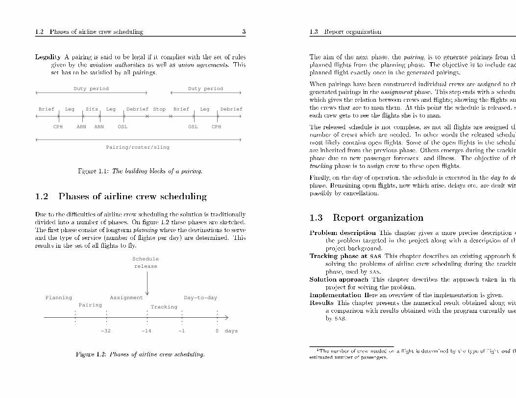
Legality A pairing is said to be legal if it complies with the set of rules

given by the aviation authorities as well as union agreements. This

set has to be satis�ed by all pairings.

LegBrief Sits Leg Debrief

CPH ARN ARN OSL

Stop Brief Leg Debrief

CPHOSL

Duty periodDuty period

Pairing/roster/sling

Figure 1.1: The building blocks of a pairing.

1.2 Phases of airline crew scheduling

Due to the di�culties of airline crew scheduling the solution is traditionally

divided into a number of phases. On �gure 1.2 these phases are sketched.

The �rst phase consist of longterm planning where the destinations to serve

and the type of service (number of �ights per day) are determined. This

results in the set of all �ights to �y.

0

Assignment

Pairing

release

Schedule

days

Planning

Tracking

Day−to−day

−14−32 −1

Figure 1.2: Phases of airline crew scheduling.

1.3 Report organization

The aim of the next phase, the pairing, is to generate pairings from th

planned �ights from the planning phase. The objective is to include eac

planned �ight exactly once in the generated pairings.

When pairings have been constructed individual crews are assigned to th

generated pairings in the assignment phase. This step ends with a schedul

which gives the relation between crews and �ights; showing the �ights an

the crews that are to man them. At this point the schedule is released, s

each crew gets to see the �ights she is to man.

The released schedule is not complete, as not all �ights are assigned th

number of crews which are needed. In other words the released schedul

most likely contains open �ights. Some of the open �ights in the schedul

are inherited from the previous phase. Others emerges during the trackin

phase due to new passenger forecasts1 and illness. The objective of th

tracking phase is to assign crew to these open �ights.

Finally, on the day of operation, the schedule is executed in the day-to-da

phase. Remaining open �ights, new which arise, delays etc. are dealt wit

possibly by cancellation.

1.3 Report organization

Problem description This chapter gives a more precise description o

the problem targeted in the project along with a description of th

project background.

Tracking phase at sas This chapter describes an existing approach fo

solving the problems of airline crew scheduling during the trackin

phase, used by sas.

Solution approach This chapter describes the approach taken in thi

project for solving the problem.

Implementation Here an overview of the implementation is given.

Results This chapter presents the numerical result obtained along wit

a comparison with results obtained with the program currently use

by sas.

1The number of crew needed on a �ight is determined by the type of �ight and th

estimated number of passengers.

5

Chapter2

Problem

description

Theproblemconsideredinthisprojectiscrewschedulingduringthetrack-

ingphase.Asdescribedinsection1.2aschedulehasalreadybeencon-

structedwhenenteringthetrackingphase.However,open�ightsarestill

aroundduringthetrackingphaseandtheproblemistoassigncrewtothese

�ights.Tobeabletosolvethisproblemtherehastobecrewavailablethat

canbeassignedtotheopen�ights.Therefore,di�erentkindsofstandby

timeareallocatedinthescheduleduringtheassignmentphase,whichcan

thenbeusedduringthetrackingandday-to-dayphases.

Agraphicalpresentationoftheproblem

isgivenon�gure2.1.On�gure

2.1(a)anopen�ightorientedviewofthescheduleisgiven�simplyshowing

theopen�ights.Noticethatopen�ightsCandDoriginatesfromthesame

�physical��ightbetweenCopenhagenandLondonwhichlackstwocrew

members.Thisshowsupinthescheduleastwodi�erentopen�ights.

On�gure2.1(b)thescheduleisshownfromacrewpointofviewwhichfor

eachcrewgivesthedi�erentactivitiesthatshehasbeenassigned.Duty

timeistimewhereacrewhasalreadybeenassignedto�ights;sheiswork-

ing.Standbyistimewherecrewcanbecalledonworkwitharelatively

shortnotice(oftenwithinanhour).Othertypesofstandbyareblank-days

andusable-time.Thedi�erenceslieinthespeci�crulesforhowandwhen

theycanbeusedtocloseopen�ights.Sparetimeisthetimewherecrewis

o�workandthereforecannotwork.Finallythereare�holes�inschedule

wherecrewisnotassignedtoaspeci�cactivity.Crew3hasaholeinher

2.1

Projectbackground

CPH

OSL

OSL

ARN

CPH

LHR

CPH

LHR

LHR

CPH

ABCD

Now

Time

EOpen flight

(a)Open�ightorientedviewofschedule

CPH

OSL

OSL

CPH

LHR

OSL

CPHARN

CPH

OSL

CPH

ARN

Cre

w

124 3

Dut

y

Spa

retim

e

Sta

ndby

Usa

ble−

tim No

Bla

nk−

days

(b)Creworientedviewofschedu

Figure2.1:Asamplescheduleshowingopen�ights(left)andcrewschedul

(right).

scheduleafterreturningtoCopenhagenfrom

Oslo.Holesmightbeuse

whenclosingopen�ights.

Allinone,standby,blank-days,usable-timeandholesinschedulearere

ferredtoasresourceperiods;timeinschedulewherecrewmightbeuse

tocloseopen�ights.Thisgivesthefollowingproblemstatement:

Closeasmanyopen�ightsaspossibleusingtheresourceperiods

allocatedinthescheduleascheaplyaspossible,withrespectto

somecostmeasure.

Ontopofthisacreworientedapproachshouldbetestedwhensolvingth

problem.Thismeansthatinformationaboutthecrewthatistoman

pairingshouldbesoughtusedwhenthepairingisgenerated.Thisisi

contrasttotheapproachdescribedabovewherepairingsaregeneratedi

thepairingphaseandassignedintheassignmentphase.

2.1

Projectbackground

TheprojecthasbeenmadeinacollaborationbetweenInformaticsan

MathematicalModelling(imm),TechnicalUniversityofDenmarkandScan

dinavianIT

Group(sig)thelatterbeing100%

ownedbyScandinavia

AirlineSystem(sas).

sighasdevelopedasystemcalledtap-aithatpriorto1998wassuccessfull

usedtosolvetheschedulingproblemduringthetrackingphase.However

2.1

Projectbackground

7

duetotheintroductionofnewunionrulestheheuristicsdeployedbytap-

aihasbecomeinvalid.From

1998andonwardsthetrackingphasehas

thereforebeendealtwithmanually.However,thecombinatorialnatureof

theproblemindicatesthatanOR-approachmightleadtonotablesavings.

tap-aihasapairinggenerationpartthathasbeensoughtusedtogenerate

pairingsofopen�ightswhichthencouldbeusedbythesta�.However,

sincenoinformationabouttheavailableresourcesinscheduleisusedit

isnotguaranteedthatthegeneratedpairingscanbeassignedtoacrew.

Practicesshowsthattheslingsgeneratedbytap-aioftendonot�twith

theresourcesinscheduleandtap-aiisnotcurrentlyusedbythesta�.

Chapter3

Literaturereview

Currently,therehasbeenmuchworkcarriedouttargetingthepairing

assignmentandday-to-dayphases.Butalmostno(published)workha

beendonedirectlytargetingthetrackingphase.Ithasonlybeenpossiblet

�ndonepaper[13]whichdealsdirectlywiththisphase.Butthetechnique

andideasusedinthepairing,assignmentandday-to-dayphasesarea

usablewhenconsideringschedulingduringtracking.

Theliteraturecanroughlybedividedinto3classes:Thosethatdealwit

thepairingandassignmentphases,theonethatdealswithtrackingan

thosethattrytosolveday-to-dayproblems.

3.1

Pairingandassignment

Theseproblemshavebeentargetedintwomainways;astwoseparate

problemsandasone.InbothcasesavariationoftheSetPartitionin

Problemisusedtoperformsomekindofselectionamongpairings:

3.1

Pairingandassignment

9

Minimize

Z=

n X j=1

c jxj

(3.1)

Subjectto

n X j=1

aijxj=1;

fori=1;:::;m

(3.2)

xjinteger;

forj=1;:::;n

(3.3)

aij

arisesfrom

amatrixA

whereeachrow

correspondstoa�ightand

eachcolumntoapairing.xj

denotesifpairing(column)jischosen,the

correspondingcostisc j.(3.2)ensuresthateach�ightisincludedexactly

onceinthesetofchosenpairings.Alternatively,asetcoveringmodelmight

bechosenwheretheequalsignin(3.2)isreplacedbyagreater-than-or-

equalsign.Theneach�ightiscoveredatleastoncebythechosenpairings.

BothmodelsareknowntobeNP-hard.However,afeasiblesolutiontothe

SetCoveringProblem

caneasilybefoundgivenitexist:Justincludeall

columnsinthesolution.Thisapproachcanobviouslynotbeusedwhen

dealingwiththeSetPartitioningProblembecauseofovercoverageofrows

isnotallowed.ThismakestheSetCoveringProblem

muchnicertowork

with.However,sinceovercoverageofrowsisallowedonemightgetmultiple

coverageof�ightsintheSetCoveringProblemformulation.

AnothercommonelementisagraphG

whichrepresentspossiblepairings.

Eachpathinthegraphrepresentsa(legal)pairingwhichthenagaincorre-

spondstoacolumninA.Somekindofcostorrestrictionisoftenintroduced

inG.

In[8]ageneticorevolutionaryalgorithm[12]isdevelopedthatsolvesthe

SetPartitioningProblemarisingfromcrewschedulingasdescribedabove.

Neitherpairingconstructionnortheassignmentofpairingstocrew

are

considered.

In[14]insteadofusingindividual�ightlegsasbuildingblocks,asetofduty

periods(see�gure1.1)isconstructed.Thesedutyperiodsarethenselected

inaSetCoveringProblemsothatasetofdutyperiodscoveringthe�ight

legsisobtained.Theselecteddutyperiodsareorganizedinagraphwhere

pathscorrespondtopairings.Theproblemissolvedbycolumngeneration

whereashortestpathalgorithmisusedonthegraphtogeneratecolumns

3.2

Tracking

1

toamasterproblem.ThisagainisaSetPartitioningProblem

withrow

representingtheselecteddutyperiodsandcolumnsrepresentingpairings

Averysimpleformoflegalityissoughtenforcedonthegeneratedpairing

throughthegraphrepresentation.Theinitialconstructionofdutyperiod

isnotconsidered,noristheassignmenttocrew.

In[4,6]agraphisconstructeddirectlyfrom

the�ightlegsandusedt

enumeratepossiblepairings.In[6]thepairingsareconstructedoncean

thenaSetPartitioningProblemissolved.In[4]agraphGk

isconstructe

foreachcrewkandapathinGk

nowrepresentsalegalpairingforcrewk

Ashortestpathproblemonthesegraphsareusedasthesubproblemin

columngenerationscheme.Themasterproblem

�again�becomesaSe

PartitioningProblem.Becauseapairingalwayshasacrewassociatedth

assignmentproblem

isalsosolved.Gk

isconstructedbyenumeratinga

possibleandlegalpairingsforcrewk.

[3]formulatesamathematicalmodelthatgivenasetofpairingPk

fo

eachcrewkselectsexactlyonepairingfromeachsetPk

sothatall�ight

arecoveredexactlyonce.Thismodelissolvedusingabranch-and-boun

technique.

In[9]aSimulatedAnnealingapproachistakentosolvetheassignmen

problem

(itisassumedthatasetofpairingsisgiven).Firstly,aninitia

assignmentofcrewtopairingsismadeusingsomeheuristic.Theneigh

bourhoodisde�nedbyeithermovingonepairingfromonecrewtoanothe

orbyswappingtwopairingsbetweentwocrew.

3.2

Tracking

Asmentionedabove,theonlypaperfounddealingdirectlywiththetrackin

phaseis[13].Firstly,itseparatestheintroducedphasesofairlinecrew

schedulingintotwometaphases;aplanningphaseandanoperationa

phase.Thisisoutlinedon�gure3.1.

3.3 Day-to-day 11

0 days

Planning Operation

PlanningPairing

Assignment

Tracking

Day−to−day

−32 −14 −1

Figure 3.1: The division of phases of crew scheduling into to

meta phases: The planning phase and the operational phase.

[13] de�nes the operational airline crew scheduling problem as that of �mod-

ifying individual monthly work schedules for airline crew members during

the operational phase of the planned schedule�.

The approach taken is column generation. The master problem is modelled

as a Set Partitioning Problem over the open �ights. The subproblem gen-

erates columns corresponding to pairings. The subproblem is formulated

as a shortest path problem on a duty graph Gk for each crew k. Each path

in the graph corresponds to a legal pairing. The cost associated with each

path in the Gk corresponds to the marginal cost of the new pairing in the

master problem.

The speci�c problem considered in this paper was that of cockpit crew.

3.3 Day-to-day

The day-to-day problem is also referred to as airline irregular operations

[15] or crew recovery [7], because it consists of targeting those problem that

arise due to disruption from maintenance problems, bad weather conditions

etc.

In [15] depth �rst search in a branch-and-bound tree is used to assign crew

to �ights that have become open due to disruption. The branch is done on

the assignment of a crew to an open �ight.

In [7] a graph Gk representing pairings is build for each crew k as an

extension of the already �own pairings by k. This is then used in a set

3.3 Day-to-day 1

covering formulation which ensures that each open �ight is covered at leas

once.

13

Chapter 4

Tracking phase at sas

This chapter describes the solution approach used currently by sas when

dealing with the tracking phase.

sas uses a program called tap-ai, based on self developed heuristics (which

will be described below) to close open �ights during the tracking phase.

Before 1998 tap-ai was able to e�ciently close open �ights. This was done

using reordering (from Danish �omdisponering�), which basically swaps

pairings in and out of the schedule, possibly changing already planned duty

(a more detailed description follows). But in 1998 a new union agreement

heavily limited the possibilities of changing planned duty time during the

tracking phase. Hence, the usefulness of this approach was limited.

tap-ai consists of two main parts: One that does the reordering, and one,

that generates pairings from the initial set of open �ights. To overcome the

di�culties of the new union agreement sig took the approach of letting tap-

ai generate pairings which could then be assigned to crew using allocated

resources in schedule (such as standby, blank-days, usable-time and �holes�)

instead of changing already planned duty � which was the case when using

reordering. Thus mirroring the pairing and assignment phases from �gure

1.2. The assignment is done manually.

In the following a more in-depth description of tap-ai will be given.

4.1 tap-ai 1

4.1 tap-ai

The pairing generation part approach of tap-ai can be divided into tw

steps; an initial pairing generation, which was the generator used befor

1998, and the (main) pairing generation. The latter which has been buil

on top of the initial pairing generation after 1998.

Both the pairing generation and the reordering parts of tap-ai uses th

initial pairing generation to build an initial set of pairings from the give

set of open �ights. Firstly, a description of this initial pairing is given

Secondly, a closer look will be taken at the reordering approach used prior t

1998, and thirdly, the main pairing generation used to day will be described

4.1.1 Initial pairing

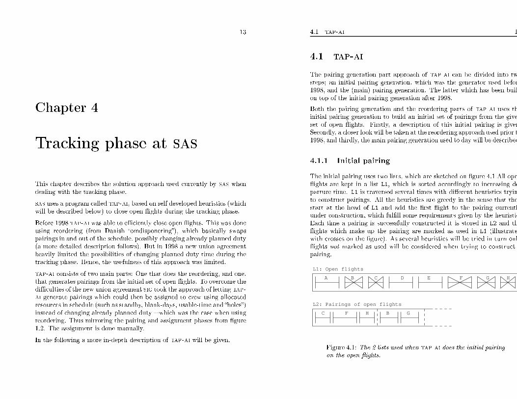
The initial pairing uses two lists, which are sketched on �gure 4.1 All ope

�ights are kept in a list L1, which is sorted accordingly to increasing de

parture time. L1 is traversed several times with di�erent heuristics tryin

to construct pairings. All the heuristics are greedy in the sense that the

start at the head of L1 and add the �rst �ight to the pairing currentl

under construction, which ful�ll some requirements given by the heuristic

Each time a pairing is successfully constructed it is stored in L2 and th

�ights which make up the pairing are marked as used in L1 (illustrate

with crosses on the �gure). As several heuristics will be tried in turn onl

�ights not marked as used will be considered when trying to construct

pairing.

L2: Pairings of open flights

L1: Open flights

A B C E G HD F

C HF B G

Figure 4.1: The 2 lists used when tap-ai does the initial pairing

on the open �ights.

4.1 tap-ai 15

As described, the initial pairing consist of a number of heuristics. They can

be divided into two main categories: A preprocessing (enforcing some rules)

and a number of heuristics which constructs pairings. The two categories

will be described next.

Preprocessing

First, a small amount of preprocessing is applied. This forces �ights to be

connected and locked1 if the �50 minute� rule2 apply. Similar the �trivsel

stop� rule3 is checked, and �ights that are required to be connected will be

connected and locked.

Heuristics

Next the following heuristics, which tries to build pairings from the �ights

in L1 are applied. The heuristics are tried successively in the order they

are listed.

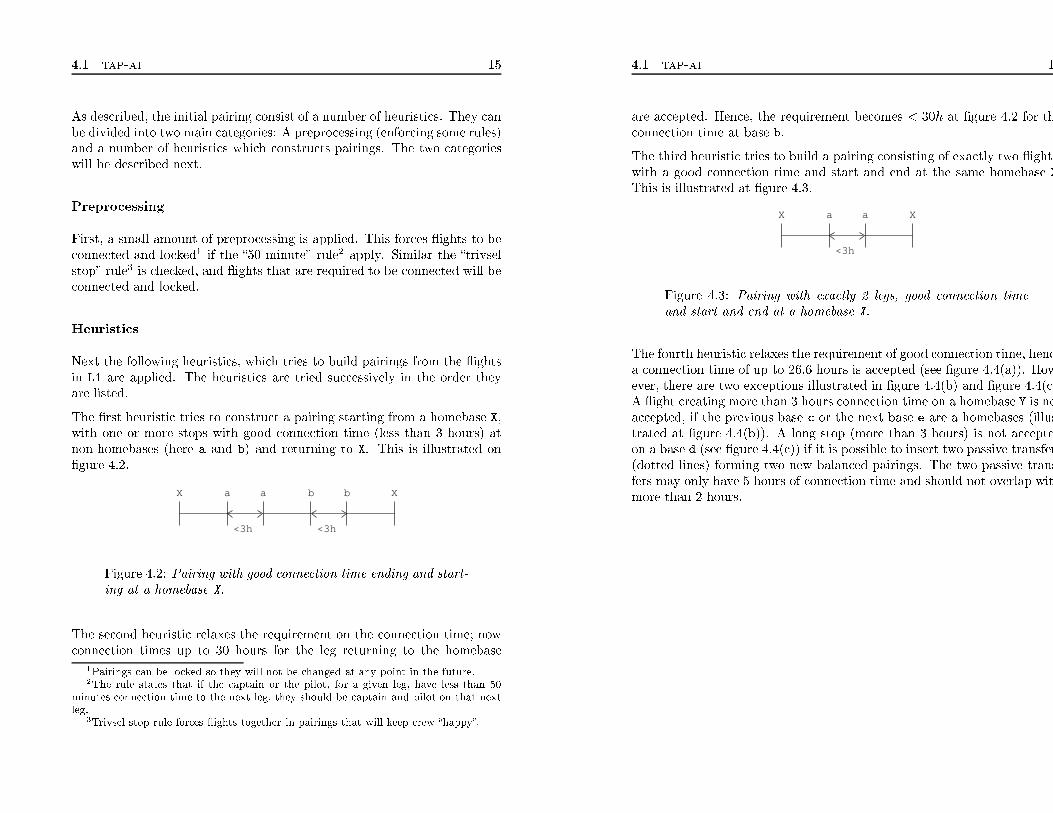
The �rst heuristic tries to construct a pairing starting from a homebase X,

with one or more stops with good connection time (less than 3 hours) at

non-homebases (here a and b) and returning to X. This is illustrated on

�gure 4.2.

<3h <3h

X a a b b X

Figure 4.2: Pairing with good connection time ending and start-

ing at a homebase X.

The second heuristic relaxes the requirement on the connection time; now

connection times up to 30 hours for the leg returning to the homebase

1Pairings can be locked so they will not be changed at any point in the future.

2The rule states that if the captain or the pilot, for a given leg, have less than 50

minutes connection time to the next leg, they should be captain and pilot on that next

leg.3Trivsel stop rule forces �ights together in pairings that will keep crew �happy�.

4.1 tap-ai 1

are accepted. Hence, the requirement becomes < 30h at �gure 4.2 for th

connection time at base b.

The third heuristic tries to build a pairing consisting of exactly two �ights

with a good connection time and start and end at the same homebase X

This is illustrated at �gure 4.3.<3h

X a a X

Figure 4.3: Pairing with exactly 2 legs, good connection time

and start and end at a homebase X.

The fourth heuristic relaxes the requirement of good connection time, henc

a connection time of up to 26.6 hours is accepted (see �gure 4.4(a)). How

ever, there are two exceptions illustrated in �gure 4.4(b) and �gure 4.4(c)

A �ight creating more than 3 hours connection time on a homebase Y is no

accepted, if the previous base c or the next base e are a homebases (illus

trated at �gure 4.4(b)). A long stop (more than 3 hours) is not accepte

on a base d (see �gure 4.4(c)) if it is possible to insert two passive transfer

(dotted lines) forming two new balanced pairings. The two passive trans

fers may only have 5 hours of connection time and should not overlap wit

more than 2 hours.

4.1 tap-ai 17

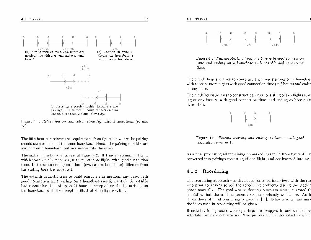
X a a b b X

<26.7h<26.7h

(a) Pairing with at most 26.6 hours con-

nection time with start and end at a home-

base X.

c Y Y e

>3h

(b) Connection time >

3 hours on homebase Y

and c or e also homebase.

c d d

<5h

e d e

<2h

<5h

d

c

(c) Inserting 2 passive �ights, forming 2 new

pairings, with at most 5 hours connection time

and no more than 2 hours of overlap.

Figure 4.4: Relaxation on connection time (a), with 2 exceptions (b) and

(c).

The �fth heuristic relaxes the requirement from �gure 4.4 where the pairing

should start and end at the same homebase. Hence, the pairing should start

and end on a homebase, but not necessarily the same.

The sixth heuristic is a variant of �gure 4.2. It tries to connect a �ight,

which starts on a homebase X, with one or more �ights with good connection

time. But now an ending on a base (even a non-homebase) di�erent from

the stating base X is accepted.

The seventh heuristic tries to build pairings starting from any base, with

good connection time, ending on a homebase (see �gure 4.5). A possible

bad connection time of up to 24 hours is accepted on the leg arriving on

the homebase, with the exception illustrated on �gure 4.4(c).

4.1 tap-ai 1

a b b c c Xd d

<24h<3h <3h

Figure 4.5: Pairing starting from any base with good connection

time and ending on a homebase with possible bad connection

time.

The eighth heuristic tries to construct a pairing starting on a homebase

with three or more �ights with good connection time (< 3 hours) and endin

on any base.

The ninth heuristic tries to construct pairings consisting of two �ights start

ing at any base a, with good connection time, and ending at base a (se

�gure 4.6).

a b b a

<3h

Figure 4.6: Pairing starting and ending at base a with good

connection time at b.

As a �nal processing all remaining unmarked legs in L1 from �gure 4.1 ar

converted into pairings consisting of one �ight, and are inserted into L2.

4.1.2 Reordering

The reordering approach was developed based on interviews with the sta

who prior to tap-ai solved the scheduling problems during the trackin

phase manually. The goal was to develop a system which mirrored th

heuristics that the sta� consciously or unconsciously would use. An in

depth description of reordering is given in [11]. Below a rough outline o

the ideas used in reordering will be given.

Reordering is a process where pairings are swapped in and out of crew

schedule using some heuristics. The process can be described as a loca

4.1 tap-ai 19

search heuristics that tries to transform a current schedule by swapping

pairings (of open �ights) into the schedule (possible) replacing other pair-

ings which then become open �ights. The hope is, that if the pairings that

are swapped into the schedule, are always �harder to cover� than the ones

they are replacing, the set of open pairings can, at some point in time, be

inserted into the schedule without replacing any other pairings.

To be able to use the above sketched local search a de�nition of �hard

to cover� and �easy to cover� pairings/�ights has to be introduced. The

following characteristics are considered:

Length Several short pairings are considered easier to cover than one long.

The hope is that small pairings can be more easily �tted into the

schedule than long ones.

Destination Flights between the three homebases are considered easy to

cover. This is natural since a huge number of personal are transported

with passive �ights between the homebases and they can be used to

cover �ights.

Departure time Pairings which are closer to operation are considered

more important to cover than pairings which are far from operation.

If it is not possible to get all open pairings closed, the set of remaining

open pairings (after the reordering process is terminated) should hopefully

be easier to cover than the initial set. Due to the last preference listed

(departure time) some important time has been achieved because open

�ights are moved forward in time.

4.1.3 Main pairing

The aim of the main pairing (in the following just referred to as pairing)

process is to produce pairings which can be covered with the resources

allocated in crew schedules. The pairings produced by the initial pairing are

optimized towards reordering of crew schedules, because it was originally

build to produce the initial set of pairings from the set of open �ights used

in the reordering part of tap-ai (as described above). Pairings used in the

reordering step are (in general) shorter than the available resources in crew

schedules. Therefore some further pairing is introduced to optimize the use

of resources.

The pairing process can run in one of two modes. In mode 1 one open �ight

is only included in one pairing (similar to the way the initial pairing works,

4.1 tap-ai 2

by marking open �ights as used). This way one can be sure, that a �ight i

not overcovered, because multiply instances of the same open �ight is no

present in several pairings.

Mode 2 does not mark �ight as used thereby producing several pairing

possible containing the same open �ight. This is dealt with by a greed

heuristics that postprocesses the set of generated pairings and selects

subset that do not contain any duplicate use of �ights.

The two di�erent modes re�ects two di�erent (and greedy) ways of dealin

with the set partitioning problem that lies beneath; generate pairings tha

covers each open �ight exactly once.

In the following descriptions of the heuristics used in the two modes ar

given.

Mode 1

Similar to the initial pairing a number of heuristics are tried in turn. The

all function on a list of pairings sorted by departure time (see �gure 4.7)

The heuristics start at the head of the list, and try to build a new pairin

constructed from pairings from the list. When a new pairing X is built it i

appended to the list and the pairing used (B, E and G) are marked as use

and ignored afterwards.

A B C D E F G X

E

G

B

Figure 4.7: List of pairings.

The �rst heuristic traverses the list of pairings looking for pairings, whic

starts or ends on a homebase. When such a pairing is found it is checked

it starts on a homebase. If it does not start on a homebase passive transfe

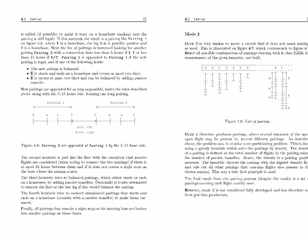
4.1 tap-ai 21

is added (if possible) to make it start on a homebase (making sure the

pairing is still legal). If this succeeds the result is a pairing like Pairing 1

on �gure 4.8, where X is a homebase, the leg X-b is possibly passive and

Y is a homebase. Next the list of pairings is traversed looking for another

pairing Pairing 2 with a connection time less than 5 hours if X=Y or less

than 15 hours if X6=Y. Pairing 2 is appended to Pairing 1 if the new

pairing is legal, and if one of the following holds:

� The new pairing is balanced.

� If it starts and ends on a homebase and covers at most two days.

� If it covers at most two days and can be balanced by adding passive

transfer.

New pairings are appended for as long as possible, under the rules described

above along with the 5/15 hours rule, forming one long pairing.

X b c Y

X!=Y: <15h

X=Y: <5h

d e fY

Pairing 1 Pairing 2

Figure 4.8: Pairing 2 are appended at Pairing 1 by the 5/15 hour rule.

The second heuristic is just like the �rst with the exception that passive

�ights are considered (when trying to connect the two pairings) if there is

at most 24 hours between them and if it does not create a night stop on

the base where the pairing starts.

The third heuristic tries to balanced pairings, which either starts or ends

on a homebase, by adding passive transfers. Optionally it is also attempted

to remove the �rst or the last leg if this would balance the pairing.

The fourth heuristic tries to connect unbalanced pairings that starts and

ends on a homebase (possible with a passive transfer) to make them bal-

anced.

Finally, all pairings that contain a night stop on the starting base are broken

into smaller pairings on those bases.

4.1 tap-ai 2

Mode 2

Mode 2 is very similar to mode 1 except that it does not mark pairing

as used. This is illustrated on �gure 4.9, which corresponds to �gure 4.7

Hence all possible combinations of pairings starting with B, that ful�lls th

requirements of the given heuristic, are built.

A B C D E F G X

G

E

Y

B B

F

G

Figure 4.9: List of pairing.

Mode 2 therefore produces pairings, where several instances of the sam

open �ight may be present in, several di�erent pairings. As describe

above, the problem now is to solve a set partitioning problem. This is don

using a greedy heuristic which sorts the pairings by density. The densit

of a pairing is de�ned as the total number of �ights in the pairing minu

the number of passive transfers. Hence, the density is a pairing qualit

measure. The heuristic chooses the pairing with the highest density �rs

and rule out all other pairings that contains �ights also present in th

chosen pairing. This way a best �rst principle is used.

The �nal result from the pairing process (despite the mode) is a set o

pairings covering each �ight exactly once.

However, mode 2 is not considered fully developed and has therefore no

been put into production.

4.2

Theprosandconsoftap-ai

23

4.2

Theprosandconsofta

p-a

i

Asalreadymentioned,theusefulnessofthereorderingpartoftap-aihas

beenheavilylimitedbythenewunionagreements.

Outofthetwomodesthatdoespairinggeneration,onlymode1hasmade

itintoproduction.Theproblemwithmode2isthatitusesahugeamount

ofmemoryandisslowcomparedwithmode1.Mode1isabletoquickly

produceasetofpairingswhichcoverstheopen�ights.However,sinceno

informationabouttheavailableresourcesinscheduleareused,thereisno

guaranteethatthegeneratedpairingscanbeassignedtocrew.Inpractice

ithasturnedout,thatthepairingsgeneratedbymode1oftendonot�t

theavailableresourcesinschedule.Thusmode1israrelyusedbythesta�

atsas.

Anotherdrawbackaretheheuristicsusedintheinitialpairing.Asone

mighthavenoticedtheyareredundantandstillresideinProlog,where

therestoftap-aiisimplementedinC/C++.Hence,maintenanceofthe

initialpairingisharderandmakingtap-aimorecomplexasawholemore

complex.

2

Chapter5

SolutionApproach

Asalreadydescribedthenewunionagreementshavemadetap-aie�ec

tivelyuseless.Theattemptmadetoovercomethesenewrestrictionswast

maketap-aiapuregeneratorwhichcouldbeusedbythesta�inthetrack

ingdepartment.However,asalreadydescribedithasnotbeensuccessfu

duetothequalityofthegeneratedpairings.Thereforesighaslookedfor

waytoimprovethegeneratedpairingsand,ifpossible,awayofassignin

crewtothegeneratedpairingsaswell.

Theusualapproachforpairingconstructiondoesnotincludeinformatio

aboutthecrewthat(atsomepointintime)isgoingto�ythepairing

Thismakessenseinthepairingphase(see�gure1.2)becausetheavailabl

resourcesintheassignmentphasearequiteuniform

amongcrew;noo

littleworkhasbeenassignedtocrewatthispoint.However,inthetrackin

phaseresourcesarespreadmorenon-uniformlyamongcrewbecausealarg

numberofpairingsalreadyhavebeenassignedtocrew.Thereforeth

pairingsthataregoingtobeassignedinthetrackingphasehastob

tailoredtothecrewthathastocoverthem.Firstly,thecrewhastob

availableintheperiodoftimethepairingcovers.Hencesheisgoingtob

onsomeformofstandby(standby,blank-day,usable-timeetc.).Secondly

thestartandendbasesofthepairinghaveto�twiththebaseatwhichth

crewisstandbyorithastobepossibletousepassivetransferstotranspor

thecrewto/from

thestart/endofthepairing.Thirdly,thepairingshav

tobelegal.

5.1 Pairing generation 25

The main idea which sig had considered was this tailoring of pairings. Gen-

erating tailored pairings for each crew also lie in the line of the reviewed

literature (see chapter 3). Here, a graph Gk which for each crew k rep-

resents the set of pairings tailored for k was widely used. Especially, in

the tracking and day-to-day phases for the reasons described above. The

pairings given by Gk was the used as columns in a Set Covering Problem or

Set Partitioning Problem. Below, a solution approach using these elements

will be presented. Firstly, the generation of pairings (Gk) will be covered

followed by the selection of the pairings each crew is to man.

5.1 Pairing generation

The goal of the pairing generation is for each crew to generate a set of

pairings that she might �y. This is conceptually done by searching through

a graph Gk for each crew k which represents the pairings constructed from

the open �ights which are tailored for k.

Firstly, a more precise de�nition of how resources are identi�ed will be

given, followed by a presentation of a number of heuristics for searching for

pairings in Gk.

5.1.1 Resources

A resource is a crew that has one or more standby allocated in her schedule.

A resource period is one or more successive standby periods in a crew

schedule. This de�nition might be extended to blank-days, usable-time

and �holes� (described in chapter 2). However, the majority of resource

time allocated in the schedule is standby and the extension might not be

straight forward due to di�erences in the rules concerning the use of the

di�erent resources. Thus only standby is considered.

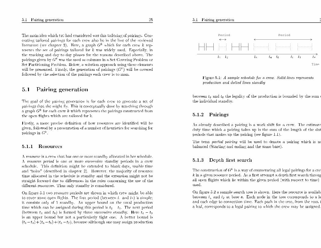
On �gure 5.1 two resource periods are shown in which crew might be able

to cover some open �ights. The �rst period (between t1 and t2) is simple;

it consists only of 1 standby. An upper bound on the total production

time which can be assigned during this period is t2 � t1. The next period

(between t3 and t8) is formed by three successive standby. Here t8 � t3

is an upper bound but not a particularly tight one. A better bound is

(t4� t3)+(t6� t5)+(t8� t7), because allthough one may assign production

5.1 Pairing generation 2

Time

Period Period

t3 t4 t5 t6 t7 t8t1 t2

Figure 5.1: A sample schedule for a crew. Solid lines represents

production and dotted lines standby

between t3 and t8 the legality of the production is bounded by the sum o

the individual standby.

5.1.2 Pairings

As already described a pairing is a work shift for a crew. The estimate

duty time which a pairing takes up is the sum of the length of the dut

periods that makes up the pairing (see �gure 1.1).

The term partial pairing will be used to denote a pairing which is no

balanced (Starting and ending and the same base).

5.1.3 Depth �rst search

The construction of Gk is a way of enumerating all legal pairings for a crew

k in a given resource period. As a �rst attempt a depth �rst search throug

all open �ights which lie within the given period (with respect to time) i

used.

On �gure 5.2 a sample search tree is shown. Here the resource is availabl

between t1 and t2 at base a. Each node in the tree corresponds to a le

and each edge to connection time. Each path in the tree, from the root t

a leaf, corresponds to a legal pairing to which the crew may be assigned.

5.1 Pairing generation 27

aaaaa

a

a

a

aaa

a

Time

aa

a

a

t1 t2

Figure 5.2: A sample search tree for the depth �rst search.

Nodes corresponds to legs and edges to connection time.

A closeup on the search tree is shown in �gure 5.3. Here four open �ights

can follow pi. Two to which it is directly connected, namely, pj and pk and

two, pl and pm, to which it is connected through passive �ights kl and km

respectively.

On table 5.1 pseudocode for a recursive depth �rst search which gener-

ates pairings is given. As arguments, DepthFirstSearch takes the pair-

ing p corresponding to the path to the current node in the search tree,

which initially is the empty pairing. Next it takes a list of partial pairings

[l1; : : : ; ln], which initially consists of one partial pairing for each open �ight

which matches the given resource period with respect to time. [l1; : : : ; ln]

is sorted by increasing departure time. Finally, Pr is the set of generated

pairings for resource period r.

Line 3-9 check the possible direct connections connecting p with an open

�ight. This corresponds to the connection between pi 7! pj and pi 7! pk on

�gure 5.3.

Line 10-17 check for possible connections between p and an open �ight

through a passive connection, which corresponds to pi 7! kl 7! pl and

pi 7! km 7! pm on �gure 5.3.

Line 19-24 check for passive �ights that would balance the current pairing.

Which corresponds to node kn on �gure 5.3.

Each of the 3 parts (line intervals) described above have more or less the

same structure. Firstly, they check if the given connection should be tried

5.1 Pairing generation 2

pi

pl

kmpm

pk

pj

kl

kn

Figure 5.3: A node pi in the searchtree with successors pj , pk pl

and pm. pl and pm are connected by two passive �ights kl and

km.

with the �okto� predicates in line 3, 10 and 19. If the connection shoul

be tried they check if a legal pairing has been generated (lines 5, 12 an

21) in which case it is saved (line 6, 13 and 22). If the connection does no

result in a legal pairing they check if the subtree beneath the current nod

should be explored (lines 7 and 14).

A more in-depth description of the di�erent predicates follows.

okToAppend(p,l,r)

okToAppend(p,l,r) is a predicate that decides if l should be appended t

p when trying to build a pairing for resource r.

On �gure 5.4 the situation is sketched. Firstly, it is checked whatever l

departure base c matches p's arrival base b and if the connection tim

between p and l, t3 � t2, lies within a prede�ned interval. Secondly, it i

checked whatever l lies within the current resource periods time interva

(t4 � t5 and t1 � t3). Finally, it is checked whatever the estimated duty o

p [ l is bigger than the estimated duty for the given resource period.

5.1 Pairing generation 29

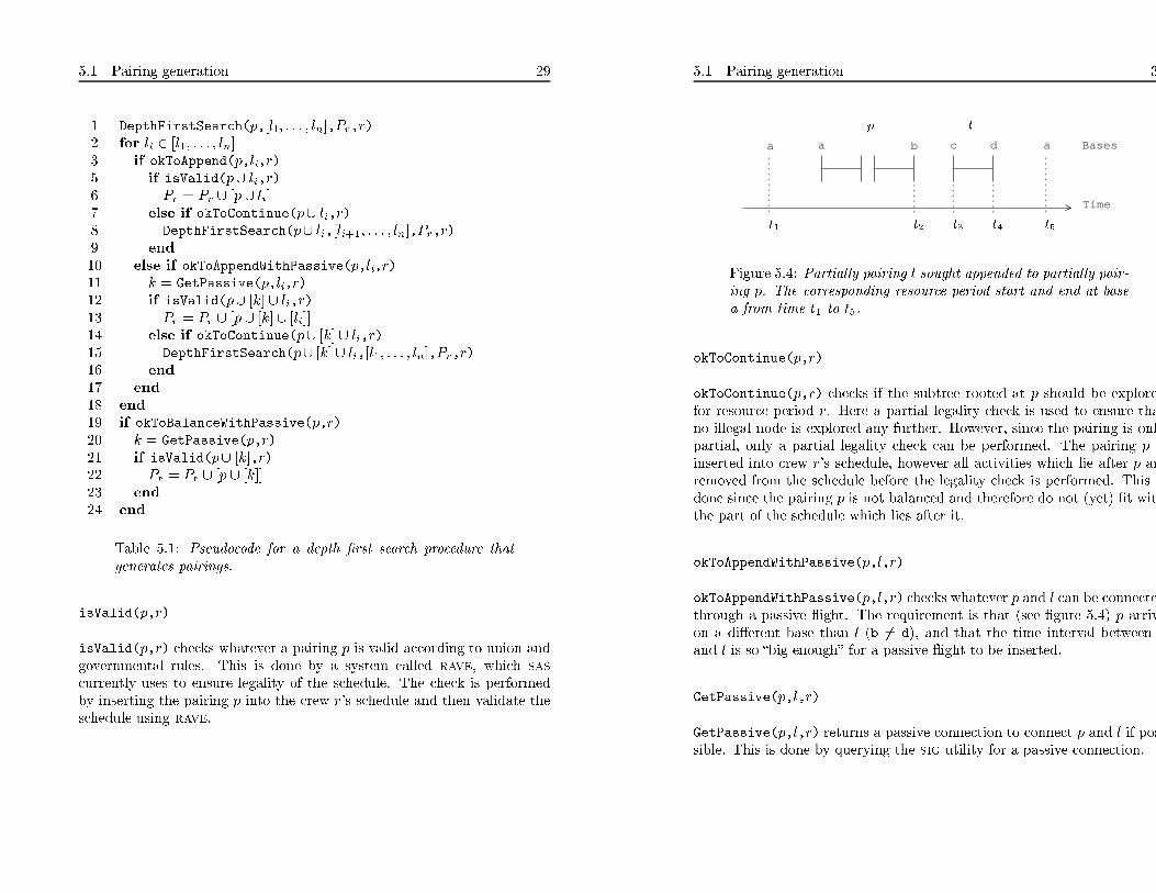
1 DepthFirstSearch(p,[l1; : : : ; ln],Pr,r)

2 for li 2 [l1; : : : ; ln]

3 if okToAppend(p,li,r)

5 if isValid(p[ li,r)

6 Pr = Pr [ [p [ li]

7 else if okToContinue(p[ li,r)

8 DepthFirstSearch(p[ li,[li+1; : : : ; ln],Pr,r)

9 end

10 else if okToAppendWithPassive(p,li,r)

11 k = GetPassive(p,li,r)

12 if isValid(p[ [k] [ li,r)

13 Pr = Pr [ [p [ [k] [ [li]]

14 else if okToContinue(p[ [k] [ li,r)

15 DepthFirstSearch(p[ [k] [ li,[l1; : : : ; ln],Pr,r)

16 end

17 end

18 end

19 if okToBalanceWithPassive(p,r)

20 k = GetPassive(p,r)

21 if isValid(p[ [k],r)

22 Pr = Pr [ [p [ [k]]

23 end

24 end

Table 5.1: Pseudocode for a depth �rst search procedure that

generates pairings.

isValid(p,r)

isValid(p,r) checks whatever a pairing p is valid according to union and

governmental rules. This is done by a system called rave, which sas

currently uses to ensure legality of the schedule. The check is performed

by inserting the pairing p into the crew r's schedule and then validate the

schedule using rave.

5.1 Pairing generation 3

Time

Basesa a b c d a

p

t1

l

t2 t3 t4 t5

Figure 5.4: Partially pairing l sought appended to partially pair-

ing p. The corresponding resource period start and end at base

a from time t1 to t5.

okToContinue(p,r)

okToContinue(p,r) checks if the subtree rooted at p should be explore

for resource period r. Here a partial legality check is used to ensure tha

no illegal node is explored any further. However, since the pairing is onl

partial, only a partial legality check can be performed. The pairing p i

inserted into crew r's schedule, however all activities which lie after p ar

removed from the schedule before the legality check is performed. This i

done since the pairing p is not balanced and therefore do not (yet) �t wit

the part of the schedule which lies after it.

okToAppendWithPassive(p,l,r)

okToAppendWithPassive(p,l,r) checks whatever p and l can be connecte

through a passive �ight. The requirement is that (see �gure 5.4) p arriv

on a di�erent base than l (b 6= d), and that the time interval between

and l is so �big enough� for a passive �ight to be inserted.

GetPassive(p,l,r)

GetPassive(p,l,r) returns a passive connection to connect p and l if pos

sible. This is done by querying the sig utility for a passive connection.

5.1 Pairing generation 31

okToBalanceWithPassive(p,r)

okToBalanceWithPassive(p,r) checks whatever it is realistic to balance

pairing p (see �gure 5.5) with a passive �ight. The requirement is that the

time between the arrival at b (t2) and the end of the given resource period

(t3) is big enough for at passive �ight and that p is not balanced already

(b 6= a).

Time

Basesa aba

t1 t3t2

p

Figure 5.5: Partially pairing l sought appended to partially pair-

ing p. The corresponding resource period start and end at base

a from time t1 to t5.

5.1.4 Depth-best �rst search

In the above description of the depth �rst search an implicit priority is used

during the search because [l1; : : : ; ln] is sorted by increasing departure time.

This way �ights with a small connection times are sought connected before

�ights with long connection times. This priority might not be optimal.

If a cost could be assigned to a pairing then at each node all possible

successors could be generated and sorted according to this cost. At each

node this would form a searchfront with a given length LSF . The nodes is

the searchfront could then be explored in turn by increasing cost.

5.1.5 Pairing cost

Estimating the cost of a pairing is not straightforward. Many factors in-

�uence on the quality of a pairing. Currently the only measurement used

by sig is the density of a pairing (introduced in section 4.1.3) which is the

total number of �ights in the pairing minus the number of passive �ights.

5.1 Pairing generation 3

This, however, is a very coarse estimate. Therefore a more �exible estimat

is introduced.

Together with sig, four aspects of a pairing have been identi�ed whic

in�uence the quality of a pairing and therefore should be re�ected in th

cost. These aspects will be introduced below.

Duty

The amount of open �ight duty which the pairing covers is important. Th

(estimated) duty of an open �ight has already been introduced in sectio

5.1.2 as the sum of the duty periods that make up the pairing. To mak

this comparable between di�erent resource periods the cost for duty is see

relatively to the estimated duty of the period the pairing is intended for:

Duty cost = 1�

Estimated duty of pairing

Estimated duty of resource period

In other words, this specify what you get (the duty covered by the pairing

relative to what you pay (the duty allocated in crew schedule). Since th

ratio grows, as the amount of duty that is covered grows the ratio actuall

measures what you gain. Therefore 1 minus the ratio is used as the cost. A

implicit assumption is made here that the remaining time in the resourc

period is not usable. Even though this might not be the case all the time

it seams reasonable during tracking. Here the goal is to use the resourc

periods allocated in the schedule and not to build up a schedule for from

scratch.

Passive �ights

The passive duty time in a pairing is also important since it basically i

time where a crew gets payed but do not work. Some passive legs in

pairing might be changed to �ordinary� legs, before crew sees the pairing

However, this is far from always the case and therefore passive �ights shoul

be avoided.

Once again a ratio is used to make the measure comparable:

Passive cost =

Estimated passive duty of pairing

Estimated duty of resource period

5.1 Pairing generation 33

Problem �ight

The notion of problem �ight arises because some open �ights are more

desirable to cover then other, or � put in other words � some open �ights

are more di�cult to cover than other.

A �ight from Copenhagen to Aalborg departing at 12.00 is easy to cover

compared with a �ight from Stockholm to Munich at 23.00. Therefore it

is more desirable to cover the second �ight than the �rst at this point in

the solution process. This idea is somewhat similar to that of reordering

(see section 4.1.2). Here the �ights are also ranked according to how big a

problem they are. And �ights that are bigger problems are sought swapped

into the schedule instead of less problematic ones.

Together with sig the following 4 aspects of an open �ight have been iden-

ti�ed which characterize a problem �ight:

� Time of departure (Early departures are problems).

� Time of arrival (Late arrivals are problems).

� Length of �ight (Long �ights are problems).

� If �ight creates a night stop (Night stops are problems).

Again a ratio is used to make the cost comparable between di�erent resource

periods.Problem Cost = 1�

Duty of problem legs

Estimated duty of resource period

Crew cover

Crew cover is the average ratio of crew which have resource periods which

matches (with respect to time) the legs in the given pairing. This gives a

rough estimate of how likely it is that the legs in the pairing can be covered

by another crew.

The cost of a pairing is a weighted sum of the introduced costs:

Cost =Duty Weight�Duty Cost+

Problem Weight� Problem Cost+

Passive Weight� Passive Cost+

Crew Cover Weight�Crew Cover Cost

5.1 Pairing generation 3

5.1.6 Searching from the �middle and out�

The search strategy forces a given partial pairing to be part of the pair

ings that are generated. This is illustrated on �gure 5.6. Here a partia

pairing from b to c is used as a starting point for 2 depth �rst searches

One searches backwards in time towards the start of the given period an

another forward in time towards the end of the period.

A modi�ed version of the depth �rst search described in section 5.1.3 i

used. The largest modi�cation is that between t1 and t2 the search has t

be backwards in time form b towards a.

a

aaa

a

aa

aa

cb

a

a

a

a

a

aa

Time

t1 t4t2 t3

Figure 5.6: A sample search tree for depth �rst searching back-

and forward from a given pairing.

5.1.7 Preprocessing of the open �ights

When constructing pairings for di�erent resource periods (di�erent crew

several open �ights will be sought connected over and over again. Therefor

a preprocessing of the open �ights where all possible successors are foun

for each �ight might improve performance. This idea forms a clone betwee

the classical approach, where all pairings are generated �rst and then crew

are assigned, and the idea that is tested in this project where crew ar

considered in the generation process.

The idea is to construct two maps which for each leg gives the possibl

direct successors and possible successors through a passive leg. Thought o

in terms of graphs the two maps represents a �meta graph� G that contain

5.2

Pairingselection

35

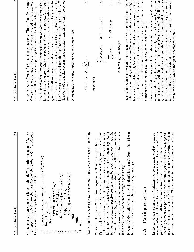
allpairingsthataregoingtobeconsidered.Thepathsrepresentedbythe

crewspeci�cgraphGk

arethenasubsetofthepathsinG.Pseudocode

forgeneratingthemapsisgivenintable5.2.

1

ConstructSuccessorMaps([l1;:::;ln],DS,PS,P)

2

forl i2

[l1;:::;l n]

3

forl j2

[li+1;:::;ln]

4

ifdirectSuccessor(l i,l j)

5

DS[li]=DS[li][

l j

6

elseifpassiveSuccessor(l i,l j)

7

PS[li]=PS[li][

l j

8

P[(l i;lj)]=GetPassive(l i,l j)

9

end

10

end

11

end

Table5.2:Pseudocodefortheconstructionofsuccessormapsforeachleg.

ConstructSuccessorMapstakes4arguments:Thelistofopen�ights

[l1;:::;ln]and3maps.DSisamapbetweenalegl iandalistofpos-

sibledirectsuccessorsofl i.

PS

mapsbetweenalegl iandthepossi-

blesuccessorsthroughapassiveleg.P

mapsapairofopenlegs(li;lj)

tothecorrespondingpassivelegthatcanbeusedtoconnectl iandl j.

directSuccessor(l i,l j)isapredicatethatindicatesifl jisapossibledi-

rectsuccessorofl i.passiveSuccessor(l i,l j)isapredicatethatindicates

ifl iandl jcanbeconnectedthroughapassiveleg.

Nowaslightlymodi�edversionofthedepth-�rstsearchfromtable5.1can

beusedtosearchtheopen�ightsgivenbythemaps.

5.2

Pairingselection

Intheprevioussectionasetofpairingshasbeenconstructedforeachre-

sourceperiod.Inthissectionwefocusontheselectionofasubsetofthose

pairingswhichwillbetheonesactually�own.Theproblem

consistsof

choosingatmostonepairingforeachresourceperiodthatthecorrespond-

ingcrewhastocover.TheproblemismodelledasaSetCoveringProblem

plussomeextraconstraints.Theseconstraintsensurethatacrewisnot

5.2

Pairingselection

3

assignedtwodi�erent�ightsatthesametime.Thisisdonebygroupin

thepairingsaccordingtothecrewtheywheregeneratedfor(seetable5.3

andthenallowatmostonepairingtobeselectedwithineachgroup.

ThechoiceofaSetCoveringProbleminfavourofaSetPartitioningProb

lemrestinthenatureofthetwoproblems.Sinceovercoverageisallowedi

theSetCoveringProblem,itisalwayseasytoconstructafeasiblesolutio

(giventhatallrowsarecoveredbyatleastonecolumneach);justinclud

allcolumns.OntheotherhandtheSetPartitioningProblemdoesnota

lowforovercoverage,andjust�ndingfeasiblesolutionmightbehard.Th

drawbackofusingthecoveringmodelisthatsome�ightsmightbecovere

severaltimes.

Amathematicalformulationoftheproblemfollows.

Maximize

Z=

m X i=1

c ixi

(5.1

Subjectto

m X i=1

aijxi�

1;

forj=1;:::;n

(5.2

X i2Ip

xi�

1;

forallcrewp

(5.3

xinonnegativeinteger

(5.4

xiisabinarydecisionvariablethatdecideswhetherpairingiisusedinth

solutionornotandc iisthecorrespondingcost.aijindicatesifopen�ight

iscoveredbypairingi.Ipisthesetofindicesforcolumnscorrespondingt

crewp.The�rstsetofconstraintsensuresthatallopen�ightsarecovere

atleastonce(5.2).Thesecondsetofconstraintsensuresthateachcrew

contributewithatmostonepairingtothesolution(5.3).

Toensurethatafeasiblesolutionalwaysexists,socalledghostcrew

ar

introduced.A

ghostcrewhasthepropertythatithasexactlyonepair

ingassociatedandthispairingcoversexactlyoneopen�ight.Henceon

ghostcrewisintroducedforeachopen�ight.Anotheruseoftheghostcrew

istocontrolthesearchprocess,sincethecostplacedonaghostcrewco

umnwilla�ecthowdesirableitistoincludenon-ghostcrewcolumnstha

coversthesamerowasthegivenghostcrewcolumn.

5.2

Pairingselection

37

Intable5.3anexampleofaprobleminstanceisgiven.Thepairingsforthe

�rstcrew,crewA,correspondstothe�rstkA

columns,crewBthenextkB

columnsandsoforth.Thelastncolumnscorrespondtotheghostcrews;

oneforeachopen�ightformingtheunionmatrix.

c 1

���

c kA

c kA

+1

���

c kA

+kB

���

c l

c l+1

���

c l+n

1

���

1

0

���

0

���

1

0

���

0

1

0

���

0

0

���

1

���

0

1

���

0

1

. . .

���

. . .

. . .

���

. . .

. . .

. . .

. . .

. ..

. . .

. . .

0

���

1

1

���

1

���

0

0

���

1

1

Table5.3:AnexampleofaninstanceoftheSetCoveringProb-

lem.Withnrowscorrespondingtoopen�ightsandm

columns

topairings.

5.2.1

Solvingthesetcoveringproblem

Therearemanypossiblestrategies(see[2]forasurvey)forsolvingthe

SetCoveringProblem.Onecouldtrytousealinearoptimizer1,oneofthe

manyheuristicsbasedonLagrangianrelaxationcombinedwithsubgradient

optimizationorsomeotherheuristicssuchasmetaheuristics.

Therearetwomajorproblemswiththeuseofalinearoptimizer.Firstly,

sig

currentlyhasnotgotone,soifthisapproachshouldbetakenthey

wouldhavetobuyone.Secondly,theproblem

whichhastobesolved

willbeverylargecontainingbetween100and1000open�ights(rows)and

allfromafewthousandupto150000pairings(columns).Theremightbe

notablesavingsintimeusingaheuristiccomparedwithanlinearoptimizer

whitproblemsofthatsize.Theadvantageofgettingtheoptimalsolution

mightbeoverlookedduetothefactthatthecostusedonlyisarough

estimate.Thecostismostlyusedasameanofguidingthesolutionprocess

ratherthanapreciseestimateofsolutioncost.Thereforethedi�erence

betweentwosolutionsthathaveaobjectvaluewithinafewprocentmight

be�invisible�tosas.

UsingLagrangianrelaxationcombinedwithsubgradientoptimizationisaf-

fordablemeasuredinrunningtime.Butsinceextrarestrictionhasbeen

1SuchasCPLEX

5.2

Pairingselection

3

introducedintothemathematicalmodelofthestandardSetCoveringProb

lem,itisnotobviousifLagrangianrelaxationcouldbeappliedsuccessfully

OntopofthisLagrangianrelaxationishardtoimplement.Thepossibl

gainwouldbeinsolutionqualitybecauseLagrangianrelaxationisknow

tooutperform

otherheuristicswhensolutionqualityismeasured.Buta

notedabovethegaininsolutionqualitymightnotbeworththetrouble.

Thedesiredcharacteristicspointinthedirectionofa(meta)heuristic

Firstly,theyareabletosolvelargeproblemswithareasonablesolutio

qualityveryfast.Secondly,theyareofteneasytoimplement.Ithasbee

possibleto�ndasetofsuccessfulapplicationsofSimulatedAnnealingo

thesetcoveringproblemandthereforeSimulateAnnealingischosen.

Intable5.4pseudocodeforthesimulatedannealing[10,1]heuristicisgiven

AsargumentsSimulatedAnnealingtakestheSetCoveringProblemSCP

thestarttemperatureT0,thecoolingfactor�andmaximum

numbero

iterationsi max.

1

SimulatedAnnealing(SCP;T0;�;maxIter)

1

XB

=;

2

cost(XB

)=1

4

X

=generateSolution(XB

,SCP)

3

fori2

0;:::;imax

and

notstop()

6

X0

=searchNeighbourhood(X;SCP)

7

Æ=cost(X0)�

cost(X)

8

$

=random[0;1[

9

ifÆ<0or$

<e

�

Æ Ti

10

X

=X0

11

ifcost(X0)<cost(XB

)

12

XB

=X0

13

end

14

end

15

Ti+1

=��

Ti

16

end

Table5.4:Simulatedannealing.

5.2

Pairingselection

39

Solutionandneighbourhood

AsolutionX

isaselectionofcolumns(pairings).X

isfeasibleifall�ights

arecoveredatleastonceandifthereexistnogroupinwhichtocolumns

areselected.

TheneighbourhoodofasolutionX

isde�nedasthesetofsolutionsthat

canbeobtainedbyrandomlydroppingdcolumnsfrom

X

andrebuilding

thesolutionwithoutreusingthedroppedcolumns.Theconstraintthatthe

droppedcolumnscannotbereusedonlyappliestonon-ghostcrewcolumns.

Thisensuresthattheneighbourhooddoesnotcontaininfeasiblesolutions.

Ifitwaspossibletoforbidtheselectionofaghostcrewcolumnafterithad

beendropped,itwouldnotbeguaranteedthatafeasiblesolutioncouldbe

constructed.Theproblem

arisesifaghostcrewcolumnisdroppedwhere

thematchingrowcannotbecoveredbyanyothercolumn.

Solutiongeneration

generateSolution(X,SCP)usesagreedyheuristictogenerateasolution

givena,possibleempty,solutionX

andtheproblemSCP.Thefunctionis

sketchedontable5.5.Itselectsatrandomanuncoveredrowj(line3)and

calculatesforeachcolumnithatcoversjtheratiobetweenthenumber

ofuncoveredrowscoveredbyiandthecostofi(line7-9).Thecolumni

thatmaximizesthisratioisincludedinthesolution(line12).Thisprocess

continuesuntilafeasiblesolutionisobtained.

Notethatonlythosecolumnsithatdoesnotful�llthepredicate

okToSelect(i,X,SCP)areconsideredinlines6-9.Therearetwocases

whereitisnotallowedtoincludecolumni:

�

Ifanothercolumnwhichisinthesamegroupasialreadyisselected

(whichcorrespondstoconstraint(5.3)fromthemathematicalformu-

lation)or

�

ifcolumniisanon-ghostcrewcolumnthathasjustbeendropped

fromthesolution(whichcorrespondstotheconstraintintroducedin

thede�nitionoftheneighbourhood).

5.2

Pairingselection

4

1

generateSolution(X,SCP)

2

whilenotfeasible(X)

3

j=selectUncoveredRow(X,SCP)

4

ratio=�

1

5

i max=�

1

6

fori2

isCoveredBy(i,j)andokToSelect(i,X,SCP)

7

ifuniqueCovers(i)

cost(i)

>ratio

8

ratio=

uniqueCovers(i)

cost(i)

9

i max=i

10

end

11

end

12

X

=X

[

i max

13

end

Table5.5:Agreedyapproachforsolutiongeneration.

Stoppingcriteria

Thefunctionstop()(intable5.4)representsthestoppingcriteria.Th

simplestpossiblemaybea�xnumberofiterations.Eventhoughthi

criteriamightseam

pooritisoftenusedinconjunctionwithsomeothe

criterion.Choosingamaximum

numberofiterationsisoftenusedtopre

determineanupperlimitonthesolutiontime.

Ifthemaximum

numberofiterationsischosenlargeenoughitisalmos

alwaysthecasethatthesolutionprocesscanbestoppedbeforethisnumbe

ofiterationsisreached.Anaturalmeasuretoapplyistolookatthelas

Literationsandobservehowtheobjectvaluehasvaried.Ifnoorlittl

variationhasbeenobservedthesolutionprocessishalted.

41

Chapter 6

Implementation

This chapter gives a short overview of the implementation. The program

has been implemented as an extension to tap-ai. The advantages using

this approach are many; �rstly, sig's existing data structures and library

functions can be used. This way pairings, �ights, schedules, crew etc.

are already implemented and ready to use together with several library

functions where the most important are the legality checking functions.

Secondly, this makes it easy to extract data from sas and use it to test

the program. The drawback is that tap-ai has been developed within

several di�erent programming paradigms: It started out as a Prolog pro-

gram, then some of the code was ported to C and lately an object oriented

approach has been used using C++. Nowadays, the program can run com-

pletely without using the parts of the program that still resides in Prolog.

As a natural choice an object oriented approach has been taken given that

sig currently has used this paradigm in the development of tap-ai.

There has been written around 9000 lines of code in this project. The code

and test data are available at imm at /home/proj/proj7/public.

In the program code for tap-ai the term sling is used which is a synonym

for pairing. Hence, to keep the terminology consistent sling has been used

instead of pairing in the code. However, to avoid confusion in this report

the term pairing is used on the subsequent �gures.

6.1 Program design 4

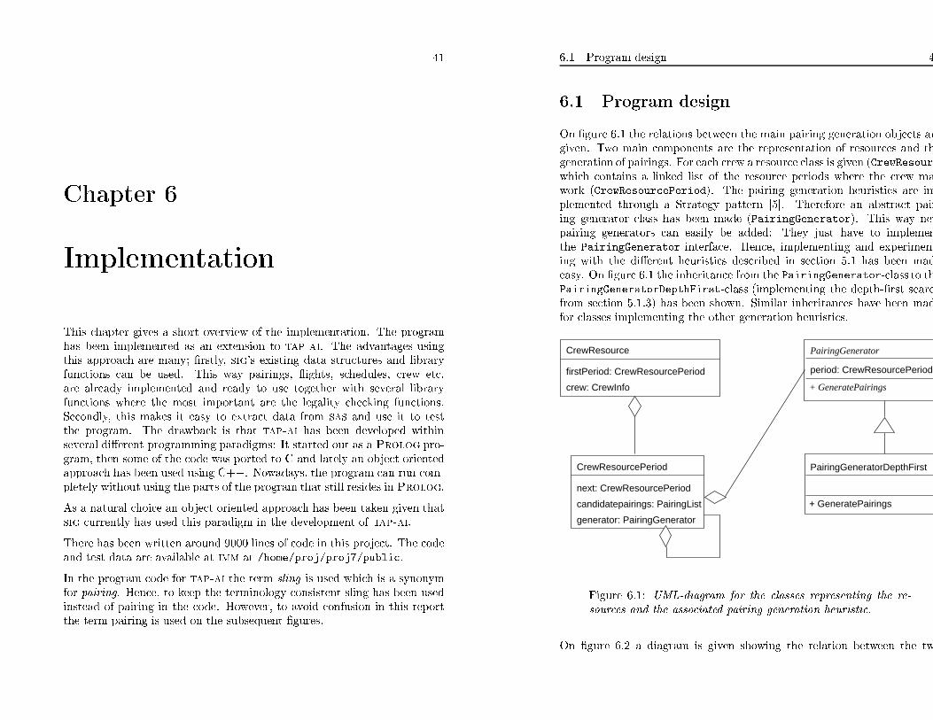
6.1 Program design

On �gure 6.1 the relations between the main pairing generation objects ar

given. Two main components are the representation of resources and th

generation of pairings. For each crew a resource class is given (CrewResour

which contains a linked list of the resource periods where the crew ma

work (CrewResourcePeriod). The pairing generation heuristics are im

plemented through a Strategy pattern [5]. Therefore an abstract pair

ing generator class has been made (PairingGenerator). This way new

pairing generators can easily be added: They just have to implemen

the PairingGenerator interface. Hence, implementing and experiment

ing with the di�erent heuristics described in section 5.1 has been mad

easy. On �gure 6.1 the inheritance from the PairingGenerator-class to th

PairingGeneratorDepthFirst-class (implementing the depth-�rst searc

from section 5.1.3) has been shown. Similar inheritances have been mad

for classes implementing the other generation heuristics.

generator: PairingGenerator

period: CrewResourcePeriod

PairingGenerator

CrewResourcePeriod

next: CrewResourcePeriod

candidatepairings: PairingList

+ GeneratePairings

CrewResource

firstPeriod: CrewResourcePeriod

crew: CrewInfo

PairingGeneratorDepthFirst

+ GeneratePairings

Figure 6.1: UML-diagram for the classes representing the re-

sources and the associated pairing generation heuristic.

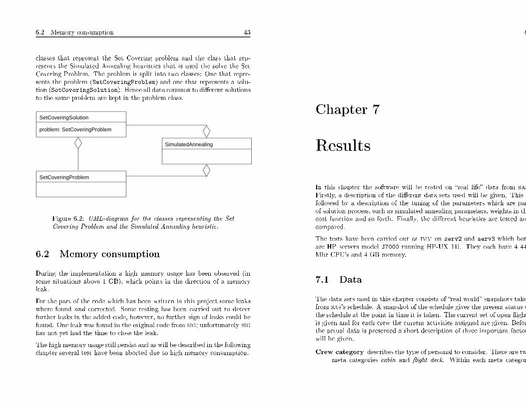
On �gure 6.2 a diagram is given showing the relation between the tw

6.2 Memory consumption 43

classes that represent the Set Covering problem and the class that rep-

resents the Simulated Annealing heuristics that is used the solve the Set

Covering Problem. The problem is split into two classes: One that repre-

sents the problem (SetCoveringProblem) and one that represents a solu-

tion (SetCoveringSolution). Hence all data common to di�erent solutions

to the same problem are kept in the problem class.

SetCoveringProblem

SetCoveringSolution

problem: SetCoveringProblem

SimulatedAnnealing

Figure 6.2: UML-diagram for the classes representing the Set

Covering Problem and the Simulated Annealing heuristic.

6.2 Memory consumption

During the implementation a high memory usage has been observed (in

some situations above 1 GB), which points in the direction of a memory

leak.

For the part of the code which has been written in this project some leaks

where found and corrected. Some testing has been carried out to detect

further leaks in the added code, however, no further sign of leaks could be

found. One leak was found in the original code from sig; unfortunately sig

has not yet had the time to close the leak.

The high memory usage still persist and as will be described in the following

chapter several test have been aborted due to high memory consumption.

4

Chapter 7

Results

In this chapter the software will be tested on �real life� data from sas

Firstly, a description of the di�erent data sets used will be given. This i

followed by a description of the tuning of the parameters which are par

of solution process, such as simulated annealing parameters, weights in th

cost function and so forth. Finally, the di�erent heuristics are tested an

compared.

The tests have been carried out at imm on serv2 and serv3 which bot

are HP servers model J7000 running HP-UX 11i. They each have 4 44

Mhz CPU's and 4 GB memory.

7.1 Data

The data sets used in this chapter consists of �real world� snapshots take

from sas's schedule. A snapshot of the schedule gives the present status o

the schedule at the point in time it is taken. The current set of open �ight

is given and for each crew the current activities assigned are given. Befor

the actual data is presented a short description of three important factor

will be given.

Crew category describes the type of personal to consider. There are tw

meta categories cabin and �ight deck. Within each meta categor

7.1

Data

45

thereareseveraldi�erentsubcategories.Asdescribedearlierthis

projectfocusesoncabincrew

andthereforethethreemaintypes

ofcabincrewareincludedinthedata.Thisisreasonablebecause

oftenacrewisquali�edtoworkasallormanyofthedi�erentsub

categorieswithinoneofthemetacategories.

Timeintervalistheperiodoftimethesnapshotcovers.Ifasmallinterval

ischosentheproblemcanbesolved�fast�becausethenumberofopen

�ightsandthenumberofcrew

areproportionalwiththeinterval

length.Butasmallintervalmightnotbesolved�good�becausethe

continuityoftheproblem.Manyopen�ightsmightlieclosetoor

crosstheendingsoftheintervalwhichmakesthem

impossibleto

cover.

Timebeforeoperation

isthenumberofdaysbetweenthedaythesnap-

shotwastakenandthe�rstdayinthesnapshot.

Inall16di�erentsnapshotshavebeentaken.Theshotshavebeendivided

into4groupsaccordingtothetimeintervaltheycover.

Ontable7.1foursnapshotsarelistedeachcoveringatimeintervalof2

days.The�rstcolumnshowsthenameoftheshot,thesecondcolumnthe

timebeforeoperation,thethirdthedates(inFebruary)thatarecovered

bytheshot.Thetwolastcolumnsshowsthenumberofcrewsandthe

numberofopen�ightsrespectively.

Name

Time

before

operation

Date

Crew

Open�ights

1

1

6.-7.

226

168

2

2

7.-8.

226

198

3

7

12.-13.

297

133

4

14

18.-19.

334

215

Table7.1:Datasnapshotfrom

5thFebruary2002.Eachshot

covers2days.

On�gure7.1thedistributionofresourceperiodsondi�erenttimeintervals

isshownforthefoursnapshotsfrom

table7.1.The�gureshowshowthe

dataclosetooperation(snapshot1and2)hasmanyshortresourceperiods

andfewlong.Thedatasetswith7and14daysbeforeoperation(snapshot

3and4)hasfewershortresourceperiodsandseverallongperiods.This

7.1

Data

4

situationarisesbecauseasoperationgetscloser,resourcesinschedulear

usedtocloseopen�ightsreducingthenumberofresourceperiodsandth

lengthoftheremainingresourceperiodsinschedule.The�top�inthe�20

25�-intervaliscausedbythefactthatsasoftenallocatesresourcestha

havethislength.

020406080100

120

140

160

180

9

periods

Est

imat

ed d

uty

(hou

rs)

Res

ourc

e pe

riods

, 5. F

ebru

ary

2002

cov

erin

g 2

days

]0-5

]]5

-10]

]10-

15]

]15-

20]

]20-

25]

]25-

30]

]30-

35]

]35-

40]

]40-

45]

]45-

1 2 3 4

Figure7.1:Numberofresourceperiodsversusresourceperiods

lengthforthedatasetfrom

table7.1.

Similartothepresentationofsnapshots1,2,3and4snapshot5,6,7,

and9arelistedintable7.2andthedistributionofresourcesperiodsi

shownon�gure7.2.

7.1

Data

47

Name

Time

before

operation

Date

Crew

Open�ights

5

2

7.-9.

294

245

6

5

10.-12.

331

212

7

8

13.-15.

358

285

8

14

19.-21.

456

209

Table7.2:Datasnapshotfrom

5thFebruary2002.Eachshot

covers3days.

020406080100

120

140

160

180

200

220

9

periods

Est

imat

ed d

uty

(hou

rs)

Res

ourc

e pe

riods

, 5. F

ebru

ary

2002

cov

erin

g 3

days

]0-5

]]5

-10]

]10-

15]

]15-

20]

]20-

25]

]25-

30]

]30-

35]

]35-

40]

]40-

45]

]45-

5 6 7 8

Figure7.2:Numberofresourceperiodsversusresourceperiods

lengthforthedatasetfrom

table7.2.

Snapshotsthatcovers4and5daysarelistedbelowintable7.3andtable

7.4withcorrespondingresourceperiodsdistributionsploton�gure7.3and

�gure7.4respectively.

7.1

Data

4

Name

Time

before

operation

Date

Crew

Open�ights

9

2

18.-21.

469

354

10

6

22.-25.

510

716

11

10

26.-1.

483

642

12

14

2.-5.

520

447

Table7.3:Datasnapshotfrom

15thFebruary2002.Eachshot

covers4days.

020406080100

120

140

160

180

9

periods

Est

imat

ed d

uty

(hou

rs)

Res

ourc

e pe

riods

, 15.

Feb

ruar

y 20

02 c

over

ing

4 da

ys

]0-5

]]5

-10]

]10-

15]

]15-

20]

]20-

25]

]25-

30]

]30-

35]

]35-

40]

]40-

45]

]45-

9 10 11 12

Figure7.3:Numberofresourceperiodsversusresourceperiods

lengthforthedatasetfrom

table7.3.

7.2

Modelparameters

49

Name

Time

before

operation

Date

Crew

Open�ights

13

2

18.-22.

553

502

14

6

22.-26.

563

899

15

10

26.-2.

555

751

16

14

2.-6.

611

512

Table7.4:Datasnapshotfrom

15.February2002.Eachshot

covers5days.

020406080100

120

140

160

180

200

9

periods

Est

imat

ed d

uty

(hou

rs)

Res

ourc

e pe

riods

, 15.

Feb

ruar

y 20

02 c

over

ing

5 da

ys

]0-5

]]5

-10]

]10-

15]

]15-

20]

]20-

25]

]25-

30]

]30-

35]

]35-

40]

]40-

45]

]45-

13 14 15 16

Figure7.4:Numberofresourceperiodsversusresourceperiods

lengthforthedatasetfrom

table7.4.

7.2

Modelparameters

Thee�ectonthesolutionfrom

thechoiceofvaluesforthedi�erentpa-

rameterswhichispartofthemodelaretestedandappropriatevaluesare

found.

7.2

Modelparameters

5

Forseveralreasonsthesetestshasonlybeencarriedoutonalimitedse

ofthesmallsnapshots.Firstly,thelongrunningtimesrangingfrom

coupleofhoursforthesmallshotsandmorethan10hoursforsomeofth

bigshotsmakestestingextremelytimeconsuming.Secondly,duetoth

memoryconsumption(asdescribedinsection6.2)ithasnotbeenpossibl

toruntestswithsomecombinationsofsnapshotandparameters.This�o

course�introducesfurtheruncertaintyregardingthechoiceofparameter

forthelargesnapshots.Hopefully,somesimilarityshouldexistamongth

snapshotsandtheparametersfoundwhentestingonthesmallsnapshot

shouldprovidegoodindicationsforthechoicesofparametersforthelarg

snapshots.

7.2.1

ParametersinSimulatedAnnealing

WhenusingSimulatedAnnealingseveralparameters(suchasstarttem

perature,coolingfactorandplateaulength)canbeadjustedandtheper

formanceoftheheuristicdependsheavilyonhowwelltheseparametersar

tuned.Intheliteratureitisoftenreportedthat�thebestparameterswa

foundaftermanyexperiments�.Thisisduetothefactthattheparameter

areheavilyproblemdependent.

Starttemperatureandcoolingfactor

AshintedinthepseudocodefortheSimulatedAnnealingprocedureth

coolingschemeisnota�plateauschedule�,wherethetemperatureiscon

stantinLsuccessiveiterationsandloweredeveryLiterations.Thereaso

isthatifvaluesforL,T0

and�aredetermined,asimilarbehaviourca

beachievedbysettingL=

1andraise�.Thereforethecoolingsched

ulesketchedinthepseudocode,wherethetemperatureisloweredateac

iteration,isusedandonlyT0

and�hastobeestimated.

On�gure7.5anaveragesolutionvalueisshownversusstarttemperatur

forthreedi�erentcoolingfactors.Foreachchoiceofcoolingfactoran

starttemperaturetheaverageistakenoverthe4datasetsfrom

table7.

(usingdepth�rstsearchforpairinggeneration).

7.2

Modelparameters

51

475

480

485

490

495

500 0.

11

1010

010

0010

000

Solution value

Sta

rt te

mpe

ratu

re

Sim

ulat

ed a

nnea

ling

para

met

ers

alph

a=0.

999

alph

a=0.

990

alph

a=0.

900

Figure7.5:SolutionvalueversusstarttemperatureT0

forthree

di�erentcoolingfactors�.

Figure7.5showsthat�=0:9and�=0:99coolstofastandbestresults

areachievedwith�=0:999.Thechoiceoftemperatureisnotthatclear;

1istolowand1000istohighbut10and100bothseemtobeacceptable.

Toshowtheimpactfrom

T0

onthesolutionprocesstworunsareshown

withdi�erentchoicesofT0.On�gure7.6theobjectvaluesforthecurrent

solutionandthebestfoundareshownversusthenumberofiterations.

Asonecanseemanyworsesolutionsareacceptedwithinthe�rst3500

iterationswhichindicatesthatthesolutionprocessmovesaroundinthe

solutionspace.Above5500iterationsthesearchconvergetowardsalocal

searchwhereonlybettersolutionsareaccepted.

7.2

Modelparameters

5

260

280

300

320

340

360

380

400

010

0020

0030

0040

0050

0060

0070

0080

0090

0010

000

Solution value

Itera

tions

Sim

ulat

ed a

nnea

ling:

Sol

utio

n va

lue

vs. i

tera

tions

.

Bes

tC

urre

nt

Figure7.6:Simulatedannealing.T0

=100and�=0:999.

On�gure7.7thestarttemperatureislowered.Nowworsesolutionsareonl

acceptedonaverysmallscaleafterthe�rst700iterations.Andabove300

iterationsthesolutionprocesslooksalmostlikepurelocalsearch.Thusth

solutionspaceisnotexploredsu�cientlyandthesolutionfoundiswors

thantheonefoundon�gure7.6withthehighertemperature.

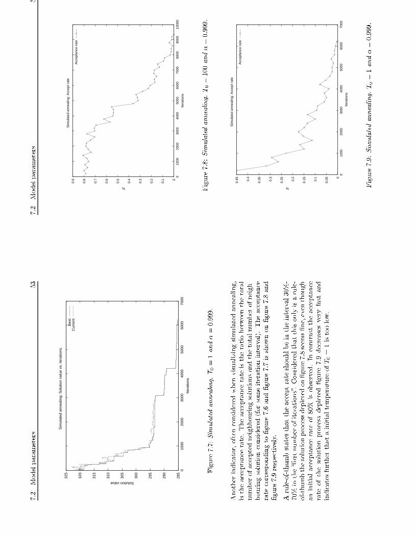
7.2

Modelparameters

53

285

290

295

300

305

310

315

320

325

010

0020

0030

0040

0050

0060

0070

00

Solution value

Itera

tions

Sim

ulat

ed a

nnea

ling:

Sol

utio

n va

lue

vs. i

tera

tions

.

Bes

tC

urre

nt

Figure7.7:Simulatedannealing.T0

=1and�=0:999.

Anotherindicator,oftenconsideredwhenvisualizingsimulatedannealing,

istheacceptancerate.Theacceptancerateistheratiobetweenthetotal

numberofacceptedneighbouringsolutionsandthetotalnumberofneigh-

bouringsolutionconsidered(forsomeiterationinterval).Theacceptance

ratecorrespondingto�gure7.6and�gure7.7isshownon�gure7.8and

�gure7.9respectively.

Arule-of-thumbstatesthattheacceptrateshouldbeintheinterval30%-

70%inthe��rstnumberofiterations�.Consideredthatthisonlyisarule-

of-thumbthesolutionprocessdepictedon�gure7.8seems�ne,eventhough

aninitialacceptancerateof80%

isobserved.Incontrasttheacceptance

rateofthesolutionprocessdepicted�gure7.9decreasesveryfastand

indicatesfurtherthatainitialtemperatureofT0

=1istoolow.

7.2

Modelparameters

5

0

0.1

0.2

0.3

0.4

0.5

0.6

0.7

0.8

0.9

010

0020

0030

0040

0050

0060

0070

0080

0090

0010

000

%

Itera

tions

Sim

ulat

ed a

nnea

ling:

Acc

ept r

ate

Acc

epta

nce

rate

Figure7.8:Simulatedannealing.T0

=100and�=0:999.

0

0.050.1

0.150.2

0.250.3

0.350.4

0.45

010

0020

0030

0040

0050

0060

0070

00

%Ite

ratio

ns

Sim

ulat

ed a

nnea

ling:

Acc

ept r

ate

Acc

epta

nce

rate

Figure7.9:Simulatedannealing.T0

=1and�=0:999.

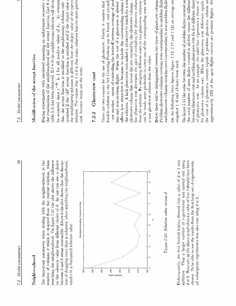
7.2

Modelparameters

55

Neighbourhood

Theimportantparameterwhendealingwiththeneighbourhood,isthe

numberofcolumnsdwhichisdroppedfrom

thecurrentsolution,when

searchingtheneighbourhood.On�gure7.10theplotshowsthein�uence

onthesolutionvaluefrom

di�erentchoiceofd.Asonecansee,achoice

between3and6seemsreasonable.Above6theplotshowsthatthedisrup-

tionofdroppingmorethan6columns,whensearchingtheneighbourhood,

resultsina�uctuatedsolutionvalue.

265

270

275

280

285

290

295

300

12

34

56

78

910

Solution value

d

Sim

ulat

ed a

nnea

ling:

Col

umns

to d

rop

Figure7.10:Solutionvalueversusd

Unfortunately,the�rstlimitedtestingshowedthatavalueofd=2was

su�cient.

Thusalargernumberofexperimentswascarriedoutusing

d=2.However,astheabovegraphshowsavalueof3or4shouldhavebeen

chosen.Tobeabletousetheresultsfromthe�rstlargesetofexperiments,

allsubsequentexperimentswasalsorunusingd=2.

7.2

Modelparameters

5

Modi�cationoftheacceptfunction

Duringexperimentswithsimulatedannealinganunfortunatepropertyo

thecombinationoftheneighbourhoodandtheacceptfunction(line9o

table5.4)hasbeenobserved.IfÆ=0theneighbouringsolutionwillalway

beacceptedsincee

�

0 Ti

is1forallpositivevaluesofTi.

Toovercom

this,theacceptfunctionismodi�edsotheneighbouringsolutiononlyi

acceptedifthe�old�acceptfunctionissatis�edandiftheobjectvalueo

theneighbouringsolutionisdi�erentfrom

theobjectvalueofthecurren

solution.ThereasonthatÆ=0isthatmanycolumnshasthesamepairin

cost,becausemanyarethesame.

7.2.2

Ghostcrew

cost

Therearetworeasonsfortheuseofghostcrew:Firstly,itensuresthat

feasiblesolutiontotheSetCoveringProblemcanbefound,andsecondly

�yetanother�meanofcontrollingthetradeo�betweencoverageofprob

lem

andnon-problem

�ights.Whenthecostofaghostcrewisalteredi

a�ectshowattractiveitbecomestoincludethecorrespondingcolumni

thesolution.Ahighghostcrewcostmakesitattractivetosearchforanon

ghostcrewcolumnthatcoverstherowcoveredbytheghostcrewcolumn.A

lowghostcrewcostdecreasesthegainofexcludingtheghostcrewcolum

fromthesolution.Byassigningdi�erentcoststotwoghostcrewcolumnsi

canbemademorepro�tabletocoveroneofthecorrespondingrowswit

anon-ghostcrewcolumnthantheother.

Belowtherewillbedistinguishedbetweentwotypesofghostcrewcolumns

Problemghostcrewcolumnscoveringrowscorrespondingtoproblem�ight

andghostcrewcolumnscoveringrowscorrespondingtonon-problem�ights

Onthefollowingthree�gures(�gure7.12,7.11and7.13)anaverageove

snapshot1,6and13havebeenused.

On�gure7.11theratiobetweenthenumberofproblem�ightscoveredan

thetotalnumberofopen�ightscoveredisplottedversusthedi�erenc

betweenghostcrewcostandproblemghostcrewcostfor�vedi�erentchoice

ofghostcrewcost.Asanexamplethesolidlinerepresentsachoiceof

forghostcrewcolumncost.Whentheghostcrewcostdi�erenceequals

thecostofaghostcrewcolumnequalsaproblem

ghostcrewcolumnan

approximately23%

oftheopen�ightscoveredareproblem

�ights.Sti

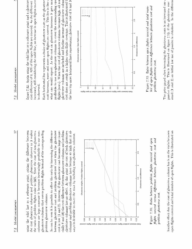
7.2

Modelparameters

57

usingthesolidlineasareferencepoint,raisingthedi�erencebetween

thecostghostcrewcolumnsandproblem

ghostcrewcolumnsto3makes

theratioofproblem

�ightsraiseto56%.Sincethecostofnon-ghostcrew

columnsarekeptconstantitbecomesincreasinglypro�tabletousenon-

ghostcrewcolumnsthatcoversproblem�ightsinsteadofthecorresponding

problemghostcrewcolumns.

Ascanbeseenitispossibletoa�ecttheratiobyincreasingthedi�erence

betweenghostcrewcostandproblem

ghostcrewcostwhentheghostcrew

costislow(1and2).However,iftheghostcrewcostbecomeslarge(espe-

cially8and16)thecostdi�erencebetweenghostcrewcolumnsandproblem

ghostcrewcolumnshasnoe�ect.Atthispointthecostofbothghostcrew

columnsandproblem

ghostcrewcolumnshavebecomesohighthatital-

waysisdesirabletocovertherowsbyincludingnon-ghostcrewcolumns.

0.150.2

0.250.3

0.350.4

0.450.5

0.550.6

0.65

00.

51

1.5

22.

53

Ratio between problem flights covered and total number of open flights covered

Gho

stcr

ew c

ost d

iffer

ence

Gho

stcr

ew w

eigh

ts: P

robl

em fl

ight

s co

vere

d

1 2 3 8 16

Figure7.11:Ratiobetweenproblem

�ightscoveredandopen

�ightscoveredversusdi�erencebetweenghostcrew

costand

problem

ghostcrewcost.

Anothere�ectthatthecostofghostcrewcolumnhasisontheratiobetween

open�ightscoveredandtotalnumberofopen�ights.Thisisillustratedon

7.2

Modelparameters

5

�gure7.12.Againusingthesolidlineasareferencepointandaghostcrew

costdi�erenceof0,40%oftheopen�ightsarecovered.Asthedi�erencei

increased,stillconsideringthesolidline,anincreaseinopen�ightscovere

isobserved.

Eachhorizontallinerepresentsachoiceofghostcrewcost;astheghostcrew

costincreases,moreandmoreopen�ightsarecovered.Thisliesinlineo

whatonewouldexpect:Asthecostonghostcrewincreasesitgetsmor

pro�tabletousenon-ghostcrewcolumnstocoverthecorrespondingope

�ights(rows).Whenthecostofghostcrewcolumnsbecomeshigh,allnon

ghostcrewcolumnsareincludedandfurtherincreaseofghostcrewcolum

costdoesnotresultinahigheropen�ightcoverage.Thisisillustratedb

thetwotopmosthorizontallinesrepresentingghostcrewcostof8and16

0.3

0.4

0.5

0.6

0.7

0.8

0.91

00.

51

1.5

22.

53

Ratio between open flights covered and total number of open flights

Gho

stcr

ew c

ost d

iffer

ence

Gho

stcr

ew w

eigh

ts: O

pen

fligh

ts c

over

ed

1 2 3 8 16Figure7.12:Ratiobetweenopen�ightscoveredandtotalnum-

berofopen�ightsversusdi�erencebetweenghostcrewcostand

problem

ghostcrewcost.

Thepricepayedwhenincreasingtheghostcrewcostsisanincreaseduseo

passive�ights.Thisisillustratedon�gure7.13;iftheghostcrewcosti

small(1and2)aninitiallowuseofpassiveisobtained.Asthedi�erenc

7.2

Modelparameters

59

betweenghostcrewcolumnsandproblem

ghostcrewcolumnsisincreased

theuseofpassiveincreasesaswell.Again,whentheghostcrewcostbe-

comeshigh(8and16)thecostofghostcrewcolumnsissohighthatitis

alwayspro�tabletocovertherowsbyincludingnon-ghostcrewcolumns.

Hencetheratioofpassiveusedbecomesconstant.

0.2

0.250.3

0.350.4

0.450.5

0.550.6

0.65

00.

51

1.5

22.

53

Ratio between passive flight used and total number of open flights covered

Gho

stcr

ew c

ost d

iffer

ence

Gho

stcr

ew w

eigh

ts: P

assi

ve u

sed

1 2 3 8 16

Figure7.13:Ratiobetweenpassive�ightsusedandopen�ights

coveredversusdi�erencebetweenghostcrewcostandproblem

ghostcrewcost.

7.2.3

Pairingcostweights

Anothermeanofcontrollingthesolutionprocessistheweightsusedin

thecostfunction(describedinsection5.1.5).Thetwomostcorrelated

weightsaretheproblem

weightandthepassiveweight;ifonewantsto

covermanyproblem�ightsonehastopayapricewhichusuallyincreases

theratioofpassive�ightsused.Firstly,theproblem

andpassiveweights

willbeexaminedfollowedbyanexaminationoftheutilizationweightand

thecrewcoverweight.

7.2

Modelparameters

6

Astestdatasnapshots1and5areusedandthenumbersreportedarea

averageoverthetwo.

Problem

andpassiveweights

On�gure7.14theratiobetweenproblem�ightscoveredandtotalnumbe

ofopen�ightscoveredisplottedversusproblem

weightfor�vedi�eren

choicesofpassiveweight.Asexpectedtheratioofproblem�ightscovere

increasesastheproblem�ightweightincreases.

0.32

0.33

0.34

0.35

0.36

0.37

0.38

0.390.

4

0.41

0.42

01

24

8

Ratio between problem flights covered and number of open flighst covered

Pro

blem

flig

ht w

eigh

t

Cos

t fun

ctio

n w

eigt

hs: P

robl

em fl

ight

s

0 1 2 4 8

Figure7.14:Ratiobetweenproblem

�ightscoveredandopen

�ightscoveredversusproblem

�ightsweight.For�vedi�erent

passiveweights.

On�gure7.15theuseofpassive�ightsisplottedversustheproblemweigh

for�vechoicesofpassiveweight.Firstly,itisnoticedthatasmallover

alldecreaseintheratioofpassiveusedcanbeobservedastheproblem

�ightweightincreases.Onemightexpectthattheuseofpassive�ight

wouldincreaseasmoreandmoreproblem

�ightsarecovered.However,

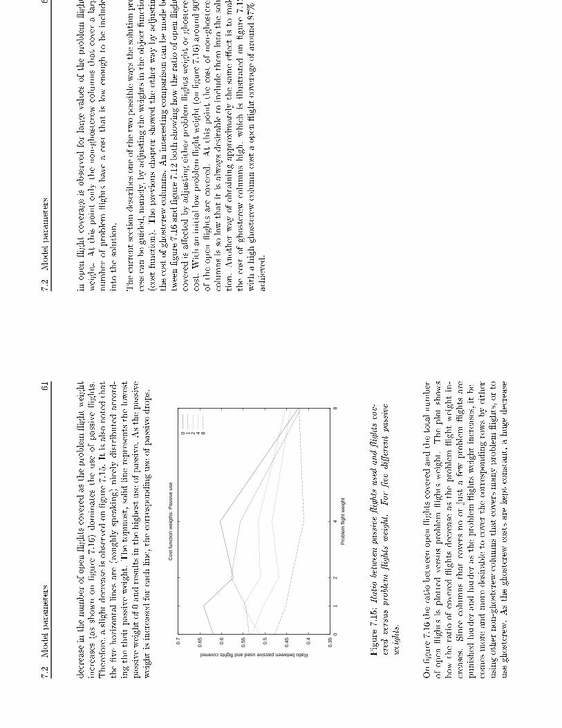
7.2

Modelparameters

61

decreaseinthenumberofopen�ightscoveredastheproblem�ightweight

increases(asshownon�gure7.16)dominatestheuseofpassive�ights.

Therefore,aslightdecreaseisobservedon�gure7.15.Itisalsonotedthat

the�vehorizontallinesare(roughlyspeaking)nicelydistributedaccord-

ingthetheirpassiveweight.Thetopmost,solidlinerepresentsthelowest

passiveweightof0andresultsinthehighestuseofpassive.Asthepassive

weightisincreasedforeachline,thecorrespondinguseofpassivedrops.

0.350.4

0.450.5

0.550.6

0.650.7

01

24

8

Ratio between passive used and flights covered

Pro

blem

flig

ht w

eigh

t

Cos

t fun

ctio

n w

eigt

hs: P

assi

ve u

se

0 1 2 4 8

Figure7.15:Ratiobetweenpassive�ightsusedand�ightscov-

eredversusproblem

�ightsweight.

For�vedi�erentpassive

weights.

On�gure7.16theratiobetweenopen�ightscoveredandthetotalnumber

ofopen�ightsisplottedversusproblem

�ightsweight.Theplotshows

howtheratioofcovered�ightsdecreaseastheproblem

�ightweightin-

creases.Sincecolumnsthatcoversnoorjustafewproblem

�ightsare

punishedharderandharderastheproblem�ightsweightincreases,itbe-

comesmoreandmoredesirabletocoverthecorrespondingrowsbyeither

usingothernon-ghostcrewcolumnsthatcoversmanyproblem�ights,orto

useghostcrew.Astheghostcrewcostsarekeptconstant,ahugedecrease

7.2

Modelparameters

6

inopen�ightcoverageisobservedforlargevaluesoftheproblem

�ight

weight.Atthispointonlythenon-ghostcrewcolumnsthatcoveralarg

numberofproblem

�ightshaveacostthatislowenoughtobeinclude

intothesolution.

Thecurrentsectiondescribesoneofthetwopossiblewaysthesolutionpro

cesscanbeguided,namely,byadjustingtheweightsintheobjectfunctio

(costfunction).Thepreviouschaptershowedtheotherwaybyadjustin

thecostofghostcrewcolumns.Aninterestingcomparisoncanbemodebe

tween�gure7.16and�gure7.12bothshowinghowtheratioofopen�ight

coveredisa�ectedbyadjustingeitherproblem�ightsweightorghostcrew

cost.Withaninitiallowproblem�ightweight(on�gure7.16)around90%

oftheopen�ightsarecovered.Atthispointthecostofnon-ghostcrew

columnsissolowthatitisalwaysdesirabletoincludethemintothesolu

tion.Anotherwayofobtainingapproximatelythesamee�ectistomak

thecostofghostcrew

columnshigh,whichisillustratedon�gure7.12

withahighghostcrewcolumncostaopen�ightcoverageofaround87%i

achieved.

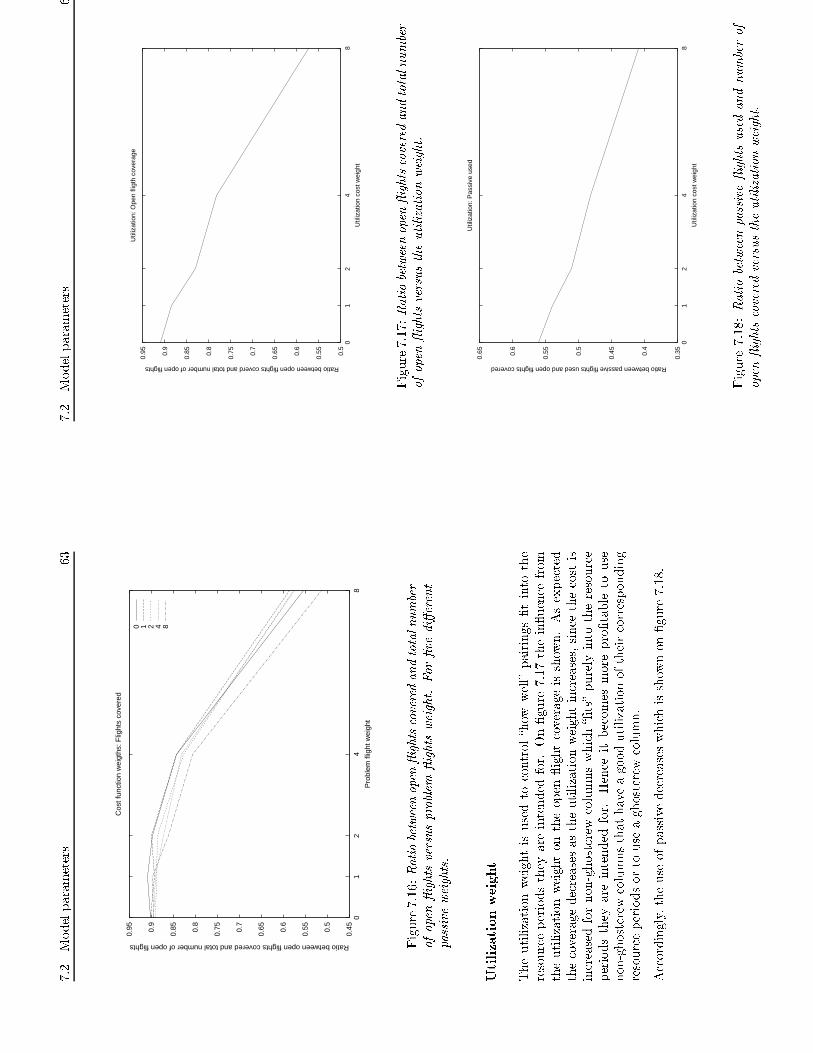
7.2

Modelparameters

63

0.450.5

0.550.6

0.650.7

0.750.8

0.850.9

0.95

01

24

8

Ratio between open flights covered and total number of open flights

Pro

blem

flig

ht w

eigh

t

Cos

t fun

ctio

n w

eigt

hs: F

light

s co

vere

d

0 1 2 4 8

Figure7.16:Ratiobetweenopen�ightscoveredandtotalnumber

ofopen�ightsversusproblem

�ightsweight.For�vedi�erent

passiveweights.

Utilizationweight

Theutilizationweightisusedtocontrol�howwell�pairings�tintothe

resourceperiodstheyareintendedfor.On�gure7.17thein�uencefrom

theutilizationweightontheopen�ightcoverageisshown.Asexpected

thecoveragedecreasesastheutilizationweightincreases,sincethecostis

increasedfornon-ghostcrewcolumnswhich��ts�purelyintotheresource

periodstheyareintendedfor.Henceitbecomesmorepro�tabletouse

non-ghostcrewcolumnsthathaveagoodutilizationoftheircorresponding

resourceperiodsortouseaghostcrewcolumn.

Accordingly,theuseofpassivedecreaseswhichisshownon�gure7.18.

7.2

Modelparameters

6

0.5

0.550.6

0.650.7

0.750.8

0.850.9

0.95

01

24

8

Ratio between open flights coverd and total number of open flights

Util

izat

ion

cost

wei

ght

Util

izat

ion:

Ope

n fli

gth

cove

rage

Figure7.17:Ratiobetweenopen�ightscoveredandtotalnumber

ofopen�ightsversustheutilizationweight.

0.350.4

0.450.5

0.550.6

0.65

01

24

8Ratio between passive flights used and open flights covered

Util

izat

ion

cost

wei

ght

Util

izat

ion:

Pas

sive

use

d

Figure7.18:Ratiobetweenpassive�ightsusedandnumberof

open�ightscoveredversustheutilizationweight.

7.2

Modelparameters

65

Crew

coverweight

Thecrewcoverweightpunishesthosepairingswhichcoveropen�ightswith

ahighcrewcover(asdescribedinsection5.1.5).Asthecrewcoverweight

isincreasedtheopen�ightscoveragedecreasesasitgetsmoreandmore

pro�tabletouseghostcrewcolumns.Thisisshownon�gure7.19.

0.81

0.82

0.83

0.84

0.85

0.86

0.87

0.88

0.890.9

01

24

8

Ratio between open flights coverd and total number of open flights

Cre

w c

over

cos

t wei

ght

Cre

w c

over

: Ope

n fli

ght c

over

age

Figure7.19:Ratiobetweenopen�ightscoveredandtotalnumber

ofopen�ightsversusthecrewcoverweight.

On�gure7.20thecorrespondinguseofpassiveisshown.Theuseincreases

becausethe�ightsthatbecomesmorepro�tabletocoveraretheones

withalow

crew

cover,whichoftenare�ightswhicharehardtocover

(oftenproblem�ights).Thisisillustratedon�gure7.21wheretheratioof

problem�ightscoveredareplotted.Hereasmallincreaseisobserved.

7.2

Modelparameters

6

0.450.5

0.550.6

0.650.7

0.75

01

24

8

Ratio between passive flights used and open flights covered

Cre

w c

over

cos

t wei

ght

Cre

w c

over

: Pas

sive

use

d

Figure7.20:Ratiobetweenpassive�ightsusedandnumberof

open�ightscoveredversusthecrewcoverweight.

0.34

0.34

5

0.35

0.35

5

0.36

0.36

5

0.37

0.37

5

01

24

8Ratio between problem flights covered and number of open flights covered

Cre

w c

over

cos

t wei

ght

Cre

w c

over

: Pro

blem

flig

ht c

over

age

Figure7.21:Ratiobetweenproblem

�ightscoveredandnumber

ofopen�ightscoveredversusthecrewcoverweight.

7.2

Modelparameters

67

7.2.4

Boundingthedepth�rstsearch

Duringthe�rstfewpilotexperimentsitbecameclearthatthesearchtree

hadtobeboundedmoreaggressivelythandescribedinthepseudocode(see

table5.1).Heretheboundingismadebyensuringtimeanddestination

matchandbyuseofthelegalitycheckingutility.However,thisdoesnot

provideane�cientlimitationofthesearchtree.Belowthenewbounds

areintroducedandtested.

Afterafew

pilotexperimentsitturnedoutthatforsomesearchtrees

severalhundredofthousandnodeswhereexplored,whichbecomesvery

timeconsuming.Asimplesolutionisanupperboundonthenumberof

searchnodestoexplore,below

calledM1.Anotheridea,whichalsois

basedonobservationsfrom

thepilotexperiments,isanupperboundon

thenumberofnodestoexplorewithoutanygenerationoflegalpairings,

below

calledM2.Forsomecrew

ahugenumberofnodesareexplored

withoutanysuccessfulpairinggeneration.Thereasonbeingthata�full�

legalitycheckcannotbecarriedoutbeforeacompletepairinghasbeen

constructed.Sincethenodesinthesearchtree(besidestheleaf-nodes)are

allpartialtheyarenotlegalbecausetheyarenotbalanced.Thereforeonly

alimitedlegalitycheckcanbeusedandtheviolationoftherulesetfor

somepairingswill�rstbediscoveredwhentheybecomebalanced.

Thetesthasbeencarriedoutonsnapshots1and5andtheresultsarethe

averageoverthesetwosnapshots.

On�gure7.22thein�uenceonthesolutiontimefrom

thechoicesofM1

andM2

areshown.ThedecisivefactorforthesolutiontimeisclearlyM1;

thechoiceofM2

hasnosigni�cantin�uenceontheoverallrunningtime.

7.2

Modelparameters

6

0

2000

4000

6000

8000

1000

0

1200

0

1400

0

1600

0

1800

0

2000

0 1000

050

000

7500

010

0000

1500

00

Solution time (seconds)

Max

imum

num

ber

of n

odes

Bou

ndin

g de

pth-

first

sea

rch:

Sol

utio

n tim

e

100

1000

1000

0

Figure7.22:SolutiontimeversusM1

forthreedi�erentchoicesofM2.

Togetacorrespondingmeasureofthein�uenceonthesolutionqualityth

solutioncostisplottedon�gure7.23andtheratioofopen�ightscovere

inthe�nalsolutionisplottedon�gure7.24.

7.2

Modelparameters

69

250

300

350

400

450 10

000

5000

075

000

1000

0015

0000

Cost

Max

imum

num

ber

of n

odes

Bou

ndin

g de

pth-

first

sea

rch:

Sol

utio

n co

st

100

1000

1000

0

Figure7.23:SolutioncostversusM1

for3di�erentchoicesofM2.

Again,themostsigni�cantfactorseemtobeM1.However,choosingahigh

valueofM2

=10000allowforasmallerchoiceofM1

=75000.Thismight

beinterpretedasfollows;byincreasingM1

youclearlygeneratemorepair-

ingsallowingforabettersolutiontotheSetCoveringproblem.However,

loweringthevalueofM1

mightbecompensatedbyincreasingthevalueof

M2.Now,insteadofgeneratingmanypairingsforsomecrew,severalother

crewwhichwasearliercuto�byM2

nowhaspairingsgenerated.

Anothermeasureofthesolutionqualityistherationofopen�ightscovered,

whichisplottedon�gure7.24.Theplotcorrespondswellwith�gure7.23;

aroundM1

=75000theplotseemto�attenoutespeciallyforthetwohigh

choicesofM2.

7.2

Modelparameters

7

0.72

0.74

0.76

0.780.

8

0.82

0.84

0.86

0.880.

9 1000

050

000

7500

010

0000

1500

00

Ratio of open flights covered

Max

imum

num

ber

of n

odes

Bou

ndin

g de

pth-

first

sea

rch:

Ope

n fli

ghts

cov

ered

100

1000

1000

0

Figure7.24:Ratioofopen�ightscoveredin�nalsolutionversus

M1

forthreedi�erentchoicesofM2.

7.2.5

Searchfrontlengthfordepth-best�rstsearch

Theimportantparameterwhenusingdepth-best�rstsearchisthelengt

LSF

ofthesearchfront.ThesearchislimitedtotheLSF-bestateachnode

AsmallvalueofLSF

willresultinaverygreedysearchthatonlyexplore

thecurrentlybestpartialpairingstherebyloweringthesolutionqualit

notable.OntheotherhandalargevalueofLSF

willcausethesearcht

exploreclosetoallsuccessorsofagivennodemakingthesearchaplai

(unbounded)depth�rstsearchandloosingthedesiredperformancegain

On�gure7.25thein�uencefrom

LSF

ontherunningtimeisshown.A

onewouldexpecttherunningtimeincreaseswithLSF;moreandmor

nodesareexplored.

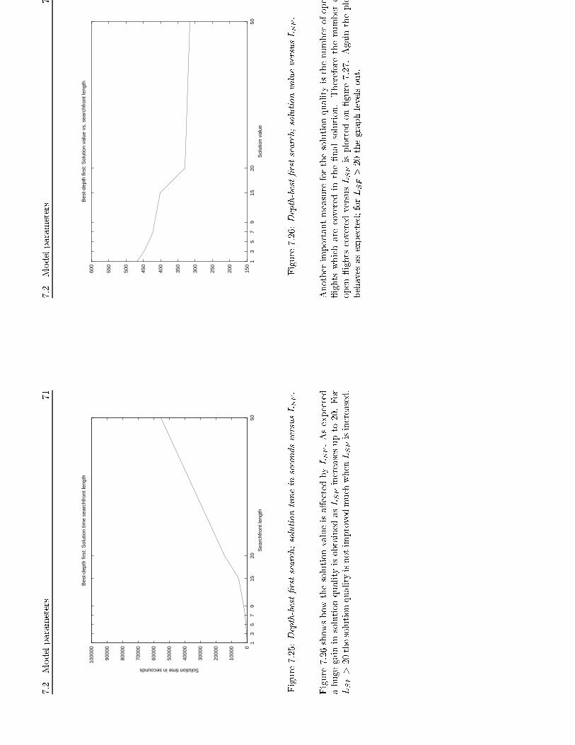
7.2

Modelparameters

71

0

1000

0

2000

0

3000

0

4000

0

5000

0

6000

0

7000

0

8000

0

9000

0

1000

00

13

57

915

2050

Solution time in secounds

Sea

rchf

ront

leng

th

Bes

t-de

pth

first

: Sol

utio

n tim

e se

arch

fron

t len

gth

Figure7.25:Depth-best�rstsearch;solutiontimeinsecondsversusLSF.

Figure7.26showshowthesolutionvalueisa�ectedbyLSF.Asexpected

ahugegaininsolutionqualityisobtainedasLSF

increasesupto20.For

LSF

>20thesolutionqualityisnotimprovedmuchwhenLSF

isincreased.

7.2

Modelparameters

7

150

200

250

300

350

400

450

500

550

600

13

57

915

2050

Sol

utio

n va

lue

Bes

t-de

pth

first

: Sol

utio

n va

lue

vs. s

earc

hfro

nt le

ngth

Figure7.26:Depth-best�rstsearch;solutionvalueversusLSF.

Anotherimportantmeasureforthesolutionqualityisthenumberofope

�ightswhicharecoveredinthe�nalsolution.Thereforethenumbero

open�ightscoveredversusLSF

isplottedon�gure7.27.Againtheplo

behavesasexpected;forLSF

>20thegraphlevelsout.

7.3

Performancetests

73

0.1

0.2

0.3

0.4

0.5

0.6

0.7

0.8

0.91

13

57

915

2050

Covered flights

Sea

rchf

ront

leng

th

Bes

t-de

pth

first

: No.

cov

ered

flig

hts

vs. s

earc

hfro

nt le

ngth

Figure7.27:depth-best�rstsearch.Numberofcoveredopen

�ightsin�nalsolutionversusLSF.

AsindicatedaboveavalueofLSF

=

20showstobeappropriate.Here

timesavingsareachievedwithouta�ectingthesolutionqualitynotable.

7.3

Performancetests

Inthissectionacomparisonofthedi�erentheuristicsdevelopedwillbe

carriedout,alongwithacomparisontheseagainstsig'sparinggeneration

mode1(asdescribedinsection4.1.3).

Usingsig'sparinggeneratorinsteadofoneofthedevelopedheuristicsis

easy:Firstly,sig'sgeneratorisusedtogeneratepairingsfrom

theopen

�ights.Secondly,foreachcrewthesubsetofthegeneratedpairingsthat

shemightmanareidenti�ed.Thisestablishesasituationsimilartothe

oneobtainedfromtheothergenerationheuristics.Hence,theSetCovering

Problemcanbeinitializedandsolvedasifoneoftheotherheuristicshad

beenused.

7.3

Performancetests

7

Belowabbreviationsforthedi�erentpairinggenerationheuristicswillb

used.Thesearegivenintable7.5.

Pairinggenerationheuristic

Abbreviation

Depth�rstsearch

dfs

Depth-best�rstsearch

dbfs

sig'spairinggenerationmode1

sig1

Depth�rstsearchwithpreprocessing

pre

Table7.5:Heuristicsandcorrespondingabbreviation.

7.3.1

Searchingfrom

�middleandout�

Thelastheuristicdescribedinchapter5wasthesearchingfrom�themid

dleandout�asitwasdescribedinsection5.1.6.However,thisheuristi

willnotbetestedanyfurtherinthischapter,duetothefact,thatthecur

rentsetupisnotsu�cient.Theheuristicstriestobuildapairinggiven

partialpairing,butinthecurrentsetupnoappropriatewayofchoosingo

constructingthispartialpairingisavailable.Asmallnumberofpilottest

havebeencarriedout,wheretheproblem�ightshavebeenusedasstartin

points.However,thisapproachproducesthesamepairingsoverandove

againandsomekindofpre-pairinghastobeintroducedtoproducesom

appropriatestartingpointsforthisheuristic.

7.3.2

d

fs

versusd

bfs

Inthissectiondfsanddbfswillbecompared.Forthelargersnapshots

lengthofLSF

=20isnotsu�cienttoboundthesearchtree:Itbecome

tootimeconsumingandforsomeofthesnapshots,thememorylimito

1GBisexceeded.Therefore,thetwoboundsintroducedforthedfsar

alsoappliedtothedbfs.TheparametersusedareLSF

=20,M1

=5000

andM1

=10000.HoweverforthedfsachoiceofM1

=25000hasbee

necessaryformostofthelargesnapshots(10,11,12,14,15and16)simpl

tostaybelowthe1GBmemorylimit.

On�gure7.28theopen�ightcoverageiscomparedfordfsanddbfs

Theexpectedgaininsolutionqualitydonotseemtoappear;onlyasma

7.3

Performancetests

75

improvementisseenforthelargeshots,however,dfshasbeenrunwith

alowervalueofM1.Hencetheobservedgainisevenlessimpressive.For

thesmallshotsdbfsperformsworsethandfs.

A100%�ightcoverageisnotexpectedsinceafractionoftheopen�ights

lieclosetoeitherthestartortheendofthesnapshot.Such�ightsmaybe

impossibletocovergiventhechosentimeinterval.

0.550.6

0.650.7

0.750.8

0.850.9

0.951

12

34

56

78

910

1112

1314

1516

Ration between open flights covered and total number of open flights

Sna

psho

t

DF

S v

s. D

BF

S: O

pen

fligh

ts c

over

age

DB

FS

DF

S

Figure7.28:dfsversusdbfs;theplotshowstheratiobetween

open�ightscoveredandtotalnumberofopen�ightsforthe16

snapshots.

On�gure7.29thesolutiontimeforthetwoheuristicsisshown.Forthe

largesnapshotsacomparisonishardtocarryoutsincethelowervalueof

M1

hasbeenusedfordfs.Hence,thebigdi�erenceinsolutiontimeisseen

forsnapshots10andabove.Forthesmallshotsitseemsliketheoverhead

introducedbysortingthesearchfrontislargerthanthegainobtainedby

boundingthesearchfront.

7.3

Performancetests

7

0

5000

1000

0

1500

0

2000

0

2500

0

3000

0

3500

0

4000

0

4500

0

5000

0

5500

0

12

34

56

78

910

1112

1314

1516

Solution time

Sna

psho

t

DF

S v

s. D

BF

S: S

olut

ion

time

DB

FS

DF

S

Figure7.29:dfsversusdbfs;solutiontimeversussnapshot

number.40000seconds�

11hours.

Theuseofpassive�ightsisshownon�gure7.30.Roughlyspeaking

loweruseofpassive�ightscanbeobservedforthedbfsthanthedfs

Thisseemsreasonablesincetheuseofpassiveisrepresentedinthecos

function.Hence,thedbfsexplorenodes,whichrepresentsalowuseo

passivebeforenodesrepresentingahighuseofpassive.

7.3

Performancetests

77

0.4

0.450.5

0.550.6

0.65

12

34

56

78

910

1112

1314

1516

Solution time

Sna

psho

t

DF

S v

s. D

BF

S: P

assi

e us

e

DB

FS

DF

S

Figure7.30:dfsversusdbfs;ratiobetweenpassiveuseand

numberopen�ightscoveredversussnapshotnumber.

Theabovetestsshows,thatthedbfsdoesnotgivethequalityimprovement

inthesolutiontobeexpected.Themainreasonforthisbeingthatthe

costfunctionhasbeenconstructedwithafullpairinginmind.Anexample

couldbe:Apartialpairingwhich(atthestartofthesearchtree)consistof

apassive�ightonlywouldbepunishedhardbythecostfunction.Itmight

notevenbeexplored,eventhoughthispartialpairingmightturnoutto

bepartofa�good�fullpairing.

7.3.3

d

bfs

versussig

1

On�gure7.31theopen�ightcoverageiscomparedforthedbfsandsig1

heuristics.Asitcanbeseen,thedbfsresultsinanotablyhighercoverage

comparedwiththesig1.Onlyforonesnapshot,number14,thesig1results

inahigheropen�ightcoverage.Asshownintable7.4snapshot14contains

thehighestnumberofopen�ightswhichmayexplainthepoorperformance.

Thisbehaviourisalsoobservedforsnapshot10whichcontainsthethird

7.3

Performancetests

7

highestnumberofopen�ights.Thereasonbeingthatthedbfsisbounded

ifthenumberofopen�ightsarelarge,largersearchtreeshavetobebuil

toincludemore�ights.However,thisispermittedbythebounds.

0.450.5

0.550.

6

0.650.

7

0.750.

8

0.850.

9

0.951

12

34

56

78

910

1112

1314

1516

Ration between open flights covered and total number of open flights

Sna

psho

t

DB

FS

vs.

SIG

1: O

pen

fligh

ts c

over

age

DB

FS

SIG

1

Figure7.31:dbfsversussig1pairinggenerationmode1;the

plotshowstheratiobetweenopen�ightscoveredandtotalnum-

berofopen�ightsforthe16snapshots.

Asmallincreaseinthecoverageforsig1canalsobeobservedasthesnap

shotnumberincreases.Asthesnapshotnumberincreases,thesizeofth

snapshotmeasuredintimeintervalalsoincrease.Asshowninsection7.1

thenumberoflargeresourceintervalsincreasesasthetimeintervalin

creases.Sosig1performancebetteronsnapshotswheretheresourcesar

lessfragmentedratherthanones,whereresourcesaremorefragmented

Thisisalsoconsistentwiththedescriptiongiveninchapter4:Theprob

lemwithsig1was,thatthepairingsgeneratedwastolongto�tthesma

fragmentedresources.

Bothsnapshot9and13,whicharetakenjust2daysbeforeoperation

resultsinhighcoverageforthedbfs.Atthispoint,resourcesarever

fragmentedandthetailoringofpairingsseemstopayo�.

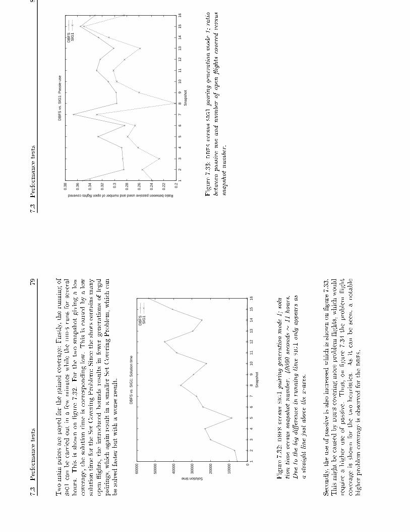
7.3

Performancetests

79

Twomainpricesarepayedforthegainedcoverage:Firstly,therunningof

sig1canbecarriedoutinafewminuteswhilethedbfsrunsforseveral

hours.Thisisshownon�gure7.32.Forthetwosnapshotgivingalow

coverage,thesolutiontimeiscorrespondinglow.Thisiscausedbyalow

solutiontimefortheSetCoveringProblem:Sincetheshotscontainsmany

open�ights,theintroducedboundsresultsinfewergenerationsoflegal

pairings,whichagainresultinasmallerSetCoveringProblem,whichcan

besolvedfasterbutwithaworseresult.

0

1000

0

2000

0

3000

0

4000

0

5000

0

6000

0

12

34

56

78

910

1112

1314

1516

Solution time

Sna

psho

t

DB

FS

vs.

SIG

1: S

olut

ion

time

DB

FS

SIG

1

Figure7.32:dbfsversussig1pairinggenerationmode1;solu-

tiontimeversussnapshotnumber.40000seconds�

11hours.

Duetothebigdi�erenceinrunningtimesig1onlyappearsas

astraightlinejustabovethex-axes.

Secondly,theuseofpassiveisalsoincreasedwhichisshownon�gure7.33.

Thismightbecausedbydbfscoveringmoreproblem�ights,whichwould

requireahigheruseofpassive.Thus,on�gure7.34theproblem

�ight

coverageisshownforthetwoheuristics.Asitcanbeseen,anotable

higherproblemcoverageisobservedforthedbfs.

7.3

Performancetests

8

0.2

0.22

0.24

0.26

0.280.

3

0.32

0.34

0.36

0.38

12

34

56

78

910

1112

1314

1516

Ratio between passive used and number of open flights covered

Sna

psho

t

DB

FS

vs.

SIG

1: P

assi

e us

e

DB

FS

SIG

1

Figure7.33:dbfsversussig1pairinggenerationmode1;ratio

betweenpassiveuseandnumberofopen�ightscoveredversus

snapshotnumber.

7.4

Preprocessing

81

0.150.2

0.250.3

0.350.4

0.450.5

0.550.6

0.65

12

34

56

78

910

1112

1314

1516

Ratio between number of problem flights covered and number of open flights covered

Sna

psho

t

DB

FS

vs.

SIG

1: P

robl

em c

over

age

DB

FS

SIG

1

Figure7.34:dbfsversussig1pairinggenerationmode1;ratio

betweenproblem�ightscoveredandnumberopen�ightscovered

versussnapshotnumber.

7.4

Preprocessing

Asseenabove,oneofthemajorlimitationsbyusingtheheuristicsisthe

runningtime.Asa�rstattemptthishasbeentargetedbyintroducinga

preprocessingoftheopen�ightsasdescribedinsection5.1.7.Theresults

aredescribedbelow.

On�gure7.35theopen�ightscoverageisshownforthefourdescribed

heuristics.Ascanbeseentheintroducingofpreprocessingincreasesthe

open�ightscoverageforthelargesnapshots.Thepreprocessingreducesthe

searchspacebyexcludingallnon-legalconnectionsfromthesearch.Thus,

morenodescanbeinvestigatedandmorelegalpairingscanbegenerated

resultinginbettersolutionstotheSetCoveringProblem.

7.4

Preprocessing

8

0.450.5

0.550.

6

0.650.

7

0.750.

8

0.850.

9

0.951

12

34

56

78

910

1112

1314

1516

Ration between open flights covered and total number of open flights

Sna

psho

t

Com

bine

d te

st: O

pen

fligh

ts c

over

age

PD

FS

DB

FS

DF

SS

IG1

Figure7.35:Open�ightscoverageversussnapshotnumberfor

thefourheuristics.

Thesolutiontimeisshownon�gure7.36.Inthis�gureanotableimprove

mentcanbeseen;preterminatesbefore20000seconds(=5.5hours)fo

allsnapshotsexceptshot10,whichisjustabove20000seconds.Compare

withasolutiontimeforsomeofthelargesnapshotsofabove11hoursfo

thedbfsthisresultmustbeconsideredsatisfying.NotethatM1

hasbee

furtherloweredfordfsonthelargesnapshotsasdescribedearlier.Hence

arelativelysmallsolutiontimeisobservedforsnapshotsnumberslarge

than10.

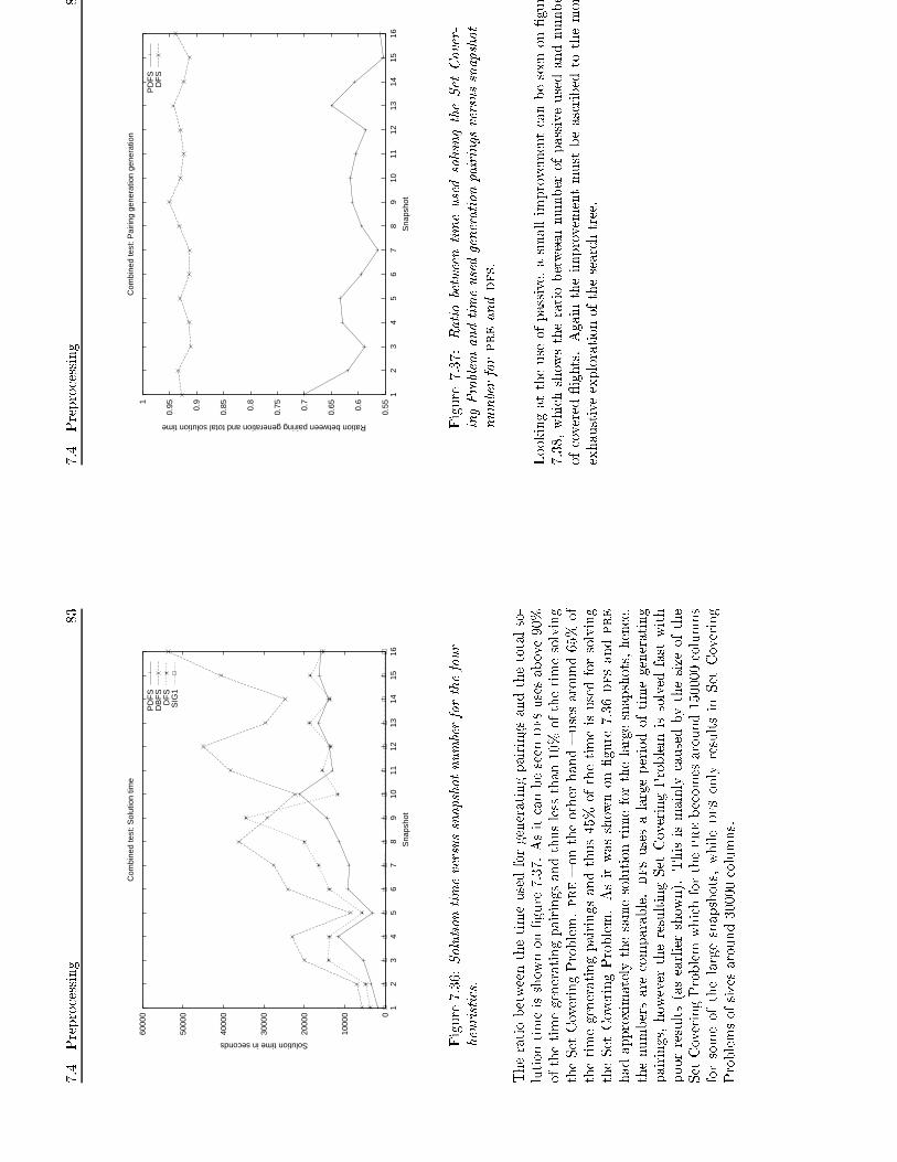
7.4

Preprocessing

83

0

1000

0

2000

0

3000

0

4000

0

5000

0

6000

0

12

34

56

78

910

1112

1314

1516

Solution time in seconds

Sna

psho

t

Com

bine

d te

st: S

olut

ion

time

PD

FS

DB

FS

DF

SS

IG1

Figure7.36:Solutiontimeversussnapshotnumberforthefour

heuristics.

Theratiobetweenthetimeusedforgeneratingpairingsandthetotalso-

lutiontimeisshownon�gure7.37.Asitcanbeseendfsusesabove90%

ofthetimegeneratingpairingsandthuslessthan10%ofthetimesolving

theSetCoveringProblem.pre�ontheotherhand�usesaround65%of

thetimegeneratingpairingsandthus45%

ofthetimeisusedforsolving

theSetCoveringProblem.Asitwasshownon�gure7.36dfsandpre

hadapproximatelythesamesolutiontimeforthelargesnapshots,hence,

thenumbersarecomparable.dfsusesalargeperiodoftimegenerating

pairings,howevertheresultingSetCoveringProblem

issolvedfastwith

poorresults(asearliershown).Thisismainlycausedbythesizeofthe

SetCoveringProblem

whichfortheprebecomesaround150000columns

forsomeofthelargesnapshots,whiledfsonlyresultsinSetCovering

Problemsofsizesaround30000columns.

7.4

Preprocessing

8

0.550.6

0.650.

7

0.750.

8

0.850.

9

0.951

12

34

56

78

910

1112

1314

1516

Ration between pairing generation and total solution time

Sna

psho

t

Com

bine

d te

st: P

airin

g ge

nera

tion

gene

ratio

n

PD

FS

DF

S

Figure7.37:RatiobetweentimeusedsolvingtheSetCover-

ingProblem

andtimeusedgenerationpairingsversussnapshot

numberforpreanddfs.

Lookingattheuseofpassive,asmallimprovementcanbeseenon�gur

7.38,whichshowstheratiobetweennumberofpassiveusedandnumbe

ofcovered�ights.Againtheimprovementmustbeascribedtothemor

exhaustiveexplorationofthesearchtree.

7.4

Preprocessing

85

0.150.2

0.250.3

0.350.4

0.450.5

0.550.6

0.65

12

34

56

78

910

1112

1314

1516

Ratio between passive use and number of open flights covered

Sna

psho

t

Com

bine

d te

st: P

assi

ve u

se

PD

FS

DB

FS

DF

SS

IG1

Figure7.38:Ratiobetweenpassiveandnumberofopen�ights

coveredversussnapshotnumberforthefourheuristics.

Toillustratethecorrespondingimpactontheproblem�ightcoverage,the

problem

�ightcoverageversussnapshotnumberisplottedon�gure7.39.

Hereitisseen,thattheproblem

�ightscoverageisnotdecreaseforthe

pre,eventhoughasmalldecreaseinpassiveusewasobservedon�gure

7.38.

7.4

Preprocessing

8

0.2

0.250.

3

0.350.

4

0.45

12

34

56

78

910

1112

1314

1516

Ratio between problem flights covered and number of open flights covered

Sna

psho

t

Com

bine

d te

st: P

robl

em c

over

age

PD

FS

DB

FS

DF

SS

IG1

Figure7.39:Ratiobetweenproblem

�ightscoveredandnum-

berofopen�ightscoveredversussnapshotnumberforthefour

heuristics.

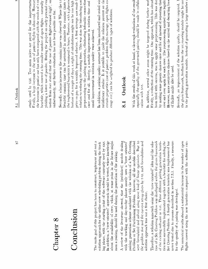
87

Chapter8

Conclusion

Themaingoalofthisprojecthasbeentoconstruct,implementandtesta

solutionapproachfortheairlinecrewschedulingproblemduringthetrack-

ingphase,withthestartingpointofthesoftwarecurrentlyusedbysas.

Inaddition,a�creworiented�approachshouldbetested,whereknowledge

abouttheavailabilityofcrew,which,atsomepointinthefuturemight

manapairing,shouldbeusedduringthegenerationofthepairing.

A

review

oftheliteratureshowed,thatthe(published)modelsdealing

withthetrackingandday-to-dayphasesmostlyusesa�crew

oriented�

pairinggenerationschemecombinedwiththesolutionofaSetCovering

Problem

orSetPartitioningProblem.However,allthemodelsdescribed

wereformulatedandsolvedusingsomekindoflinearoptimizer.Dueto

theproblemsizeandthecurrentsetupgivenbysas,suchformulationand

solutionapproachwasnota�rstchoice.

Therefore,asolutionapproachusingthe�creworiented�ideaandthesolu-

tionofaSetCoveringProblemwasdevelopedwithinthegivenframework

oftheexistingsoftwareatsas.Threedi�erentpairinggenerationheuris-

ticsweresuccessfullyimplementedtogetherwithaheuristicforsolvingthe

SetCoveringProblem.Afourthgenerationheuristicwasimplementedbut

nevertestedduetoreasonsdescribedinsection7.3.1.Finally,ameasure

forthequalityofapairingwasdeveloped.

Thenumericalresultsshowedasubstantialincreaseinthenumberofopen

�ightscoveredusingthenewheuristicscomparedwiththesoftwarecur-

8.1

Outlook

8

rentlyusedbysas.

Twomainpricesarepayedforthisimprovement

Firstly,alargeincreaseintheuseofpassive�ightsisobserved.However

theincreaseinpassiveusehasonlybeencomparedwiththeresultsofsas

heuristic,whichcoveredafarsmallernumberofopen�ights�naturally

yieldingaloweruseofpassive.Duringtheprojectanearlypersonaleva

uationfrom

sasstatedthattheuseofpassive�ights�seemedhigh�,an

unfortunately,anyfurtherevaluationhasnotbeenpossiblesofar.

Secondly,alargeincreaseintherunningtimewasobserved:Wherethesa

heuristicrunningtimecanbemeasuredinminutestherunningtimeso

theimplementedheuristicsismeasuredinhours.However,withaplannin

horizonofacoupleofdays,anightofcalculationsmightnotbetoohigh

pricetopayforanotablyimprovedsolution.A�rstattemptwasmadei

relationtoreducingtherunningtime.Thiswasdonebyintroducingsom

preprocessingtothepairinggeneration,eliminatinginfeasibleconnection

onceandforall.Hereby,anotableimprovementinsolutiontimeand

smallimprovementinsolutionqualitywereachieved.

Inaddition,apairingqualitymeasurehasbeenintroducedandtestedwit

satisfactoryresults:Itispossibletoguidethesolutionprocesssotha

certainproperties(useofpassive,problem�ightcoverage,open�ightscov

erageetc.)canbeweightedtoproducedi�erenttypesofsolutions.

8.1

Outlook

Withtheresultsofthisworkathand,athoroughevaluationoftheresult

especiallythequalityofthegeneratedpairingshouldbemadeincollabo

rationwithsas.

Inaddition,severalotherareasmightbetargetedduringfurtherwork

Firstly,areductionoftherunningtime.Oneapproach,whichhasalread

beentriedwithsuccess,wastoapplysomepreprocessing.Thiswasdon

bymakingsomegenericchoicesonceandforallinsteadofrepeatingthem

overandoveragainforeachcrew.Thepreprocessingapplieduseslegality

However,morerestrictivechoicesbasedonthearrivalanddepartingbase

of�ightsmightalsobeused.

Secondly,animprovementofthesolutionqualityshouldbetargeted.I

thegivenframework,feedbackfromthesetcoveringmodulemightbeuse

inthepairinggenerationmodule.Insteadofgeneratingalargenumbero

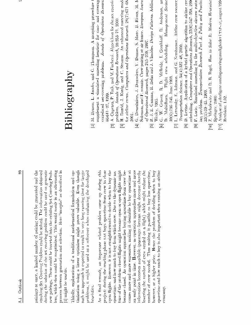
8.1

Outlook

89

pairingsatonce,alimitednumberofpairingcouldbegeneratedandthe

resultingSetCoveringProblemcouldbesolved.Theinformationobtained

duringthesolutionofthesetcoveringproblem

couldbeusedtogenerate

newpairings.ThesecouldbeinsertedintotheexistingSetCoveringProb-

lem,whichthencouldbereoptimized.Thiswouldresultinanalternating

processbetweengenerationandselection.Here�morphs�asdescribedin

[1]mightbeusable.

Thirdly,explorationsofatraditionalmathematicalformulationandop-

timizationusingalinearoptimizermightprovevaluable.Eventhough

suchanapproachisexpectedtoresultinverylongrunningtimeforlarger

problems,itmightbeusedasareferencewhenevaluatingthedeveloped

heuristics.

Asa�nalremark,animportantrelatedproblem

cameupduringthis

project;duringthetrackingphasesasbuyssparetimefrom

crewtoclose

open�ights.However,itisnotstraightforwardtodecidewhentobuythe

sparetime,andhowmuchtobuyfromwhichcrew.Duetothedynamicna-

tureoftheproblemclosed�ightsmightbecomeopenoropen�ightsmight

becomeclosed.Asoperationapproachesbuyingsparetimefrom

crewbe-

comesmoreandmoreexpensive,makingitdesirabletobuysparetimeat

anearlypointintime.However,asoperationapproachesmoreandmore

informationbecomesavailable(passengerforecastmightdecreasethereby

loweringthenumberofcrewneededona�ight)whichmightreducethe

numberofcrewneeded.Thusmakingitpossibletobuylesssparetime,

however,atahigherprice.Hencetheproblem

ofdecidingwhentobuy

sparetimeandhowmuchtobuyisalsoimportantwhenrunninganairline

company.

9

Bibliography

[1]M.Brusco,L.Jacobs,andG.Thompson.Amorphingproceduret

supplementasimulatedannealingheuristicforcost-andcoverage

correlatedset-coveringproblems.

AnnalsofOperationsResearch

86:611�27,1999.

[2]A.Caprara,P.Toth,andM.Fischetti.Algorithmsforthesetcoverin

problem.AnnalsofOperationsResearch,98:353�71,2000.

[3]H.Dawid,J.Konig,andC.Strauss.Anenhancedrosteringmode

forairlinecrews.ComputersandOperationsResearch,28(7):671�688

2001.

[4]G.Desaulniers,J.Desrosiers,Y.Dumas,S.Marc,B.Rioux,M.M

Solomon,andF.soumis.Crewpairingatairfrance.EuropeanJourna

ofOperationalResearch,pages245�259,1997.

[5]R.J.E.Gamma,R.HelmandJ.Vlissides.DesignPatterns.Addiso

Wesley,1995.

[6]G.W.Graves,R.D.McBride,I.Gershko�,D.Anderson,an

D.Mahidhara.

Flightcrew

scheduling.

ManagementSceince

39(6):736�745,June1993.

[7]L.Lettovsky,E.Johnson,andG.Nemhauser.Airlinecrewrecovery

TransportationScience,34(4):337�48,2000.

[8]D.Levine.Applicationofahybridgeneticalgorithm

toairlinecrew

scheduling.ComputersandOperationsResearch,23(6):547�558,1996

[9]P.Lucic.Simulatedannealingforthemulti-objectiveaircrewroster

ingproblem.TransportationResearchPartA:PolicyandPractice

33(1):19�45,1999.

[10]Z.MichalewiczandD.B.Fogel.HowtoSolveIt:ModernHeuristics

Springer,2000.

[11]Analyseafyderligereomdisponeringsmulighederitap-ai,august1994

Revision:1.02.

BIBLIOGRAPHY

91

[12]C.R.Reeves.Geneticalgorithmsfortheoperationsresearcher.IN-

FORMS,9(3):231�249,1997.

[13]M.Stojkovic,F.Soumis,andJ.Desrosiers.Theoperationalairline

crewschedulingproblem.TransportationScience,32(3):232�45,1998.

[14]P.Vance,C.Barnhart,E.Johnson,andG.Nemhauser.Airlinecrew

scheduling:anewformulationanddecompositionalgorithm.Opera-

tionsResearch,45(2):188�200,1997.

[15]G.Wei,G.Wu,andM.Song.Optimizationmodelandalgorithm

forcrewmanagementduringairlineirregularoperations.Journalof

CombinatorialOptimization,1(3):305�21,1997.