robustness in train scheduling master thesis imm, dtu · robustness in train scheduling master...
TRANSCRIPT
Robustness in train scheduling
Master thesis
IMM, DTU
Mads Andreas Hofman
Line Frølund Madsen
Project number 72
September 2005
Abstract
In this project robustness in train scheduling is examined. The project is conducted for DSB S-tog
because the current situation is influenced by a large amount of disturbances which cause delays
and low regularity. The aim of this project is to help DSB S-tog in the development of more robust
timetables. The robustness analysis is performed by comparing different already existing and new
timetables using simulation. The approach of simulation of timetables is new in connection with DSB
S-tog.
A generic model of the S-train network is modelled and implemented using the simulation tool Arena.
The model can simulate all arrivals and departures of the trains in the entire network during a day.
The model includes an implementation of three different recovery methods where trains are turned at
a station prior to the end station, replaced at the central station or entire lines are cancelled in order
to eliminate delays.
Distributions of the delays occurring at the stations in the S-train network are generated from historical
data for the experiments. A number of experiments are conducted and investigated. Experiments
include examination of the effect of the different recovery methods, investigation of the consequences
of delays and comparison of how different features in the timetables affect the robustness.
The results from the simulation show that generally the robustness decreases as the number of lines
in the timetable increases. Furthermore it is proven that the number of lines is not the only important
aspect when developing robust timetables. Buffer times at the terminal stations have a significant
impact on the robustness and it is also shown that the amount of necessary buffer needed to create a
robust timetable is limited. The allocation of buffer times is important since all lines should be able
to recover using buffer times. Furthermore line structure also turns out to have an impact on the
robustness.
Finally two totally new timetables with new line structures are developed in this project. They both
generally achieve an improved robustness.
Resume
Dette projekt omhandler robusthed i køreplaner. Projektet er udarbejdet for DSB S-tog, fordi de er
i en situation, hvor store forsinkelser fører til en lav regularitet. Formalet med dette projekt er at
hjælpe DSB-S-tog med at generere mere robuste køreplaner. Robusthedsanalysen er udført ved at
sammenligne forskellige køreplaner ved hjælp af simulation. Indgangsvinklen med at bruge simulation
er ny for DSB S-tog.
En generisk model af S-togs netværket er modelleret og implementeret i simulationsprogrammet Arena.
Modellen kan simulere alle ankomster og afgange i hele netværket over en dag. Ydermere er tre
forskellige genopretningsmetoder inkluderet i modellen; en hvor toge bliver vendt før endestationen,
en hvor toge bliver erstattet pa Københavns hovedbanegard og en metode, hvor hele linier bliver aflyst.
De forsinkelser, der bliver paført i modellen følger fordelinger, der er genereret udfra historisk data.
Flere forskellige forsøg er udført og evalueret. Der er eksperimenteret med hvilken indflydelse de tre gen-
opretningsmetoder har pa forskellige køreplaner, hvordan forskellige forsinkelser pavirker regulariteten
og forskellige køreplaner bliver sammenlignet i forhold til robusthed.
Resultaterne fra simulationen viser, at jo flere linier en køreplan indeholder, jo lavere bliver robust-
heden. Det viser sig ydermere, at mange andre faktorer har indflydelse pa robustheden. Buffertid pa
endestationerne har for eksempel stor indflydelse pa robustheden af en køreplan. Det viser sig ogsa,
at fordelingen af buffertid er vigtig og at der er en øvre grænse for, hvor meget ekstra buffer tid der
er nødvendig, for at lave en robust køreplan. Derudover har liniestrukturen i køreplanen en effekt pa
robustheden.
To helt ny køreplaner med en anderledes linestrukturer er ogsa udviklet. Disse giver begge en forbedret
robusthed.

Acknowledgment
This project is made in cooperation with DSB S-tog. We would like to thank the department of
production planning at DSB S-tog in general. Everybody have been very helpful. Specifically we
would like to thank Jens Clausen, Julie Jespersen, Morten N. Nielsen and Claus Ørum-Hansen for
their interest in the project.
Finally we thank our supervisor Jesper Larsen from IMM DTU.
Mads Andreas Hofman Line Frølund Madsen
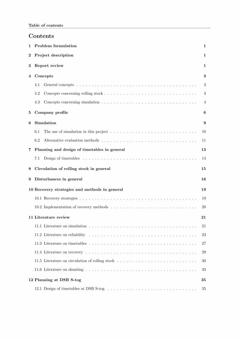
Table of contents
Contents
1 Problem formulation 1
2 Project description 1
3 Report review 1
4 Concepts 3
4.1 General concepts . . . . . . . . . . . . . . . . . . . . . . . . . . . . . . . . . . . . . . . 3
4.2 Concepts concerning rolling stock . . . . . . . . . . . . . . . . . . . . . . . . . . . . . . 3
4.3 Concepts concerning simulation . . . . . . . . . . . . . . . . . . . . . . . . . . . . . . . 4
5 Company profile 6
6 Simulation 9
6.1 The use of simulation in this project . . . . . . . . . . . . . . . . . . . . . . . . . . . . 10
6.2 Alternative evaluation methods . . . . . . . . . . . . . . . . . . . . . . . . . . . . . . . 11
7 Planning and design of timetables in general 13
7.1 Design of timetables . . . . . . . . . . . . . . . . . . . . . . . . . . . . . . . . . . . . . 14
8 Circulation of rolling stock in general 15
9 Disturbances in general 16
10 Recovery strategies and methods in general 19
10.1 Recovery strategies . . . . . . . . . . . . . . . . . . . . . . . . . . . . . . . . . . . . . . 19
10.2 Implementation of recovery methods . . . . . . . . . . . . . . . . . . . . . . . . . . . . 20
11 Literature review 21
11.1 Literature on simulation . . . . . . . . . . . . . . . . . . . . . . . . . . . . . . . . . . . 21
11.2 Literature on reliability . . . . . . . . . . . . . . . . . . . . . . . . . . . . . . . . . . . 23
11.3 Literature on timetables . . . . . . . . . . . . . . . . . . . . . . . . . . . . . . . . . . . 27
11.4 Literature on recovery . . . . . . . . . . . . . . . . . . . . . . . . . . . . . . . . . . . . 29
11.5 Literature on circulation of rolling stock . . . . . . . . . . . . . . . . . . . . . . . . . . 30
11.6 Literature on shunting . . . . . . . . . . . . . . . . . . . . . . . . . . . . . . . . . . . . 33
12 Planning at DSB S-tog 35
12.1 Design of timetables at DSB S-tog . . . . . . . . . . . . . . . . . . . . . . . . . . . . . 35
Table of contents
13 Circulation of rolling stock at DSB S-tog 37
13.1 Rolling stock at DSB S-tog . . . . . . . . . . . . . . . . . . . . . . . . . . . . . . . . . 37
13.2 Circulation plan . . . . . . . . . . . . . . . . . . . . . . . . . . . . . . . . . . . . . . . 37
14 Disturbances at DSB- S-tog 42
14.1 Regularity and reliability . . . . . . . . . . . . . . . . . . . . . . . . . . . . . . . . . . 42
14.2 Causes of disturbances at DSB- S-tog . . . . . . . . . . . . . . . . . . . . . . . . . . . 42
15 Recovery strategies and methods at DSB S-tog 45
15.1 Recovery strategies . . . . . . . . . . . . . . . . . . . . . . . . . . . . . . . . . . . . . . 45
15.2 Recovery implementation methods and practical requirements . . . . . . . . . . . . . . 47
16 Arena and description of the first models 48
16.1 Arena . . . . . . . . . . . . . . . . . . . . . . . . . . . . . . . . . . . . . . . . . . . . . 48
16.2 Description of Model 1 . . . . . . . . . . . . . . . . . . . . . . . . . . . . . . . . . . . . 52
16.3 Description of Model 2 . . . . . . . . . . . . . . . . . . . . . . . . . . . . . . . . . . . . 55
16.4 Animation . . . . . . . . . . . . . . . . . . . . . . . . . . . . . . . . . . . . . . . . . . . 59
17 Description of the final model 61
17.1 Main model . . . . . . . . . . . . . . . . . . . . . . . . . . . . . . . . . . . . . . . . . . 64
17.2 Station submodel . . . . . . . . . . . . . . . . . . . . . . . . . . . . . . . . . . . . . . . 65
17.3 Regularity . . . . . . . . . . . . . . . . . . . . . . . . . . . . . . . . . . . . . . . . . . . 69
17.4 Reliability . . . . . . . . . . . . . . . . . . . . . . . . . . . . . . . . . . . . . . . . . . . 71
17.5 Recovery Methods . . . . . . . . . . . . . . . . . . . . . . . . . . . . . . . . . . . . . . 71
17.6 Read/Write . . . . . . . . . . . . . . . . . . . . . . . . . . . . . . . . . . . . . . . . . . 80
17.7 Animation . . . . . . . . . . . . . . . . . . . . . . . . . . . . . . . . . . . . . . . . . . . 80
17.8 Delays in the model . . . . . . . . . . . . . . . . . . . . . . . . . . . . . . . . . . . . . 81
18 Verification and validation of the final model 83
18.1 Validation and assumptions . . . . . . . . . . . . . . . . . . . . . . . . . . . . . . . . . 83
18.2 Verification . . . . . . . . . . . . . . . . . . . . . . . . . . . . . . . . . . . . . . . . . . 85
19 Development of timetables for experiments 87
19.1 General procedure when developing and implementing a timetable . . . . . . . . . . . 97
20 Experiments 100
Table of contents
20.1 Introduction . . . . . . . . . . . . . . . . . . . . . . . . . . . . . . . . . . . . . . . . . . 100
20.2 Fundamental conditions for the experiments . . . . . . . . . . . . . . . . . . . . . . . . 102
21 Experiments with recovery methods for individual timetables 104
21.1 Timetable from 2003 (10 lines) . . . . . . . . . . . . . . . . . . . . . . . . . . . . . . . 105
21.2 Timetable for 2006 (9 lines) . . . . . . . . . . . . . . . . . . . . . . . . . . . . . . . . . 106
21.3 Proposed timetable with 10 lines . . . . . . . . . . . . . . . . . . . . . . . . . . . . . . 108
21.4 Combination timetable . . . . . . . . . . . . . . . . . . . . . . . . . . . . . . . . . . . . 109
21.5 Timetable with 11 and 12 lines . . . . . . . . . . . . . . . . . . . . . . . . . . . . . . . 109
22 Other experiments 111
22.1 Experiments with delay . . . . . . . . . . . . . . . . . . . . . . . . . . . . . . . . . . . 111
22.2 Experiments with more buffer time at end stations . . . . . . . . . . . . . . . . . . . . 115
22.3 Homogeneous stopping pattern . . . . . . . . . . . . . . . . . . . . . . . . . . . . . . . 119
22.4 Even distribution of tracks on København station . . . . . . . . . . . . . . . . . . . . . 120
22.5 Numbers in queues . . . . . . . . . . . . . . . . . . . . . . . . . . . . . . . . . . . . . . 120
23 Comparison of timetables 124
23.1 Comparison with delays and without recovery . . . . . . . . . . . . . . . . . . . . . . . 124
23.2 Comparison with recovery methods . . . . . . . . . . . . . . . . . . . . . . . . . . . . . 126
24 Conclusion on the experiments 131
25 Further research 133
25.1 Further development of the model . . . . . . . . . . . . . . . . . . . . . . . . . . . . . 133
25.2 Further experiments . . . . . . . . . . . . . . . . . . . . . . . . . . . . . . . . . . . . . 134
26 Conclusion 135
A Evaluation of simulation using Arena 136
B Output file 138
C Station numbers 143
D Dwell times 144
E Running times 145
F Station types 146
Table of contents
G Sequence 147
H Delay distribution 148
I Departure times in the plan with 12 lines 149
J Additional results 151
J.1 Experiments with recovery methods for individual timetables . . . . . . . . . . . . . . 151
J.2 Other experiments . . . . . . . . . . . . . . . . . . . . . . . . . . . . . . . . . . . . . . 153
J.3 Comparison of timetables . . . . . . . . . . . . . . . . . . . . . . . . . . . . . . . . . . 155
1 Problem formulation page 1
1 Problem formulation
This project is made in cooperation with DSB S-tog because they have a situation with unstable
timetables. The timetable without any modifications is only used a few days every year, the rest of
the time the timetable is modified because of unpredictable disturbances. These changes can be of
smaller or bigger dimensions, but a lot of work is put into the modifications of the timetable. The goal
for DSB S-tog is to be able to develop more robust timetables.
2 Project description
The objective of this project is to gain knowledge about the construction of robust timetables. This
is done by testing certain hypotheses regarding the stability and robustness of timetables. A robust
timetable should be able to recover from disturbances without having to re-arrange the whole plan.
Robust means that the performance of the system is less sensitive to deviations from the scheduled
timetable. Robustness is measured by categorizing a timetable according to a regularity measure,
concerning percentage departures on time but also how well the original timetable can be re-established
when disturbances have occurred.
In the process of planning a new timetable, one way of constructing a robust timetable could be to
create a number of different plans and then use simulation to determine which timetable is the most
robust. This process is very time consuming and therefore not suitable in the short term planning
process. In this project timetables with different features will be examined, and the results should
help ease the process of developing robust timetables. The timetables will be examined by building a
simulation model of the train network and investigating the results from different simulation scenarios.
The aim of this project is to get an impression of what effect different features in timetables have
on the robustness. Robustness of timetables will be measured by systematically simulating multiple
timetables affected by disturbances. The main objective is to indicate factors in the construction of
timetables, which influence the robustness of the plan. The affected timetables also have to be re-
established in order to evaluate how well they recover. A secondary objective of the project is to study
different approaches for recovering, once a disturbance has occurred. The idea is to test and compare
different recovery methods. A final purpose of the project is to investigate the simulation tool Arena.
3 Report review
The first phase of the project concerns the process of gaining knowledge about relevant subjects such
as simulation, railways, disturbances and recovery methods. In chapter 4 different concepts concerning
robustness, railways and simulation are presented. A company profile of DSB S-tog is given in chapter 5.
This chapter is followed by an examination of simulation in general and alternative evaluation methods
in chapter 6. Furthermore it is described why simulation is used to evaluate timetables in this project.
Design of timetables is examined in chapter 7, circulation of rolling stock in chapter 8, disturbances and
3 Report review page 2
delays in chapter 9, and finally recovery strategies and recovery implementation methods are described
in chapter 10. These four chapters address the general cases, the specific situation at DSB S-tog is
described later in the report. Existing literature about railways, simulation, reliability and recovery
strategies is studied to gain knowledge about terminology, research results from already completed
projects and also to get ideas for the modelling and experiment phases in this project. Summaries
of the studied articles are given in chapter 11. In the chapters 12 to 14 the subjects of design of
timetables, circulation of rolling stock, disturbances and delays and finally recovery strategies and
recovery implementation specific for DSB S-tog are examined.
The second phase of the project involves the simulation tool Arena. A model of the S-train network
will be developed in Arena. This is an important phase, because an additional objective in the project
is to study the simulation tool Arena and also because the more precise the model the more useful
the results of the later simulation will be. A description of the features in Arena and the modelling
process is given in the chapters 16 to 18.
The next phase is the process of gathering data for the experiments. The data needed for the experi-
ments are timetables with different features according to robustness and costumer service. Since DSB
S-tog have not made bigger changes in the timetables over the past 10 years, only a few very different
timetables are completely developed and directly available for this project. Therefore a part of the
project concerns developing new timetables. The timetables used for the experiments are examined in
chapter 19.
The fourth phase of the project is the simulation phase. In this phase different timetables are simulated
and experiments with disturbances and different recovery methods are conducted. Furthermore a
number of hypotheses regarding robustness are examined. The results of this phase are the actual
objectives of the project. This phase is described in the chapters 20 to 23.
The final phase is the evaluation and conclusion of the experiments and the project.
The data used in the experiments are included on the attached CD-rom.
4 Concepts page 3
4 Concepts
In this chapter some useful concepts are described. These will be used throughout the report. The
concepts are inspired from the literature, but since the meanings of some of the concepts are somewhat
diverse, the specific interpretation in this report is given.
4.1 General concepts
Robustness: Robust means that the performance of the system is less sensitive to deviations from the
scheduled timetable.
Regularity : Regularity is calculated as the percentage of departures on time.
Reliability : Reliability measures the number of actual departures from the stations compared to the
scheduled number of departures.
Disturbance: A disturbance is typically defined as a delay above a certain size e.g. more than 2.5
minutes lateness.
4.2 Concepts concerning rolling stock
Rolling stock : Trains are often described as rolling stock.
Train unit : A train unit is a number of carriages and a locomotive. Different subtypes of train units
might have different numbers of carriages.
Train type: Train type depends on e.g. the type of fuel the train uses or the age of the trains.
Train series and lines: A train series is defined by two terminal stations and all the stations in between.
A train line is covering a train series but the train running the line does not necessarily stop at all the
stations between the terminal stations.
Shunting : Sometimes during the day, for example outside rush hour, not all the available rolling stock
is used. To fully use the railway infrastructure by the running trains, the redundant trains are parked
in a shunt yard. The process of parking a train is called shunting. In this project shunting covers both
turning at terminal stations and actual parking of trains.
Marshalling : Marshalling is the procedure of either connecting or separating train units to generate
larger or smaller trains e.g. before and after the rush hour. Marshalling generally includes shunting of
the train units before connection or after separation.
Merging : Merging of lines is the action of switching between lines i.e. the train covering one line is
changed to covering another line, at a terminal during the circulation. Merging has the purpose of
reducing waiting time at the end stations and thereby reducing the total number of trains necessary
to run a plan.
Infrastructure: The infrastructure is defined as the entire network on which the trains are applied.

4.3 Concepts concerning simulation page 4
The infrastructure includes the stations, the tracks, the shunt yards, the signals etc.
Headways: The time between two consecutive trains traversing a point in the network. Minimum
headway is the minimum time between consecutive trains, which must be observed according to
safety. Minimum headways are sometimes referred to as safe headways. Planned headways are the
times between the departures for the different lines in the timetable.
Dwell time and running time: The dwell time is the time a train is waiting at a station i.e. the duration
of the stop at a station. The running time is the scheduled driving time from one station to another
(or between two points in the network).
Buffer time: Buffer time, also referred to as slack time, is the extra time which can be incorporated
into the timetable to be able to maintain scheduled departure and arrival times when delays occur.
Cycle time: The period of time it takes for a train to complete a tour from a terminal station and
back to the same terminal station.
Primary and secondary delays: Delays can be split into two categories. When disturbances occur on
running times or dwell times the resulting delays are called primary delays. Primary delays are initial
delays caused on a train from the outside and not by other trains. To reduce the delays the timetables
contain buffer time. But when buffer time is too small a cause of delay on a train may give rise to a
conflict with another train. These delays are called secondary delays. Secondary delays are delays of
trains caused by earlier delays of other trains. Primary delays are also called source delays. Secondary
delays are also referred to as knock-on delays.
Repositioning trip: Transportation of trains without passengers. Also referred to as dead heading.
4.3 Concepts concerning simulation
Simulation model : A simulation model is a computer model of a real system, with the purpose of
illustrating the behaviour of a well-defined system.
Simulation: Simulation is to solve a problem by experimenting with a simulation model. A batch
simulation is a series of simulations, where a series of experiments are run, to solve a given problem.
Static vs. dynamic simulation: Time does not play a role in static simulation but does in dynamic
simulation. Most operational models are dynamic.
Continuous vs. discrete simulation: In a continuous simulation the state of the system can change
continuously over time e.g. water running out of a tank. The basis of the continuous simulation is that
the simulation time is increased by one constant time increment at each simulation step. After each
time increment, the state changes occurred during the previous time interval are calculated. When
continuous simulation follows the clock it is called Real-time simulation. In a discrete simulation
changes can occur only at separated points of time. Discrete simulation is controlled by events, and
the state changes are updated after every event. Sometimes elements of both types are combined in a
simulation.
4.3 Concepts concerning simulation page 5
Stochastic vs. deterministic simulation: A Stochastic simulation involves randomness or probability.
Stochastic simulation can be used to e.g. analyse the effect of certain faults (randomness) applied to
the system. A deterministic simulation model is not influenced by these external factors. Deterministic
simulation is often used to illustrate a system for the sake of e.g. learning.
Iconic simulation models vs. logical simulation models: An iconic model is a physical replica or scale of
the system. A logical model is a mathematical model which builds on approximations and assumptions
about the way the system will work. If the logical model is valid it should reflect the actual behaviour
of the real system.
Macroscopic vs. microscopic simulation: A simulation model is categorized as either macroscopic or
microscopic depending on the level of detail. If the simulation model is an exact representation of
the real system the model is microscopic, but if details like signals, weather or human behavior are
omitted the simulation level is macroscopic. In the case where all materialistic details are implemented
and only human behavior is omitted the level of detail is called mesoscopic.
5 Company profile page 6
5 Company profile
In this chapter a description of the company DSB S-tog will be given. Figures and statistics are mainly
taken from the DSB S-tog Annual Report 2004 [5].
DSB S-tog A/S is a company within the DSB Group, the Danish State Railways (DSB), the company
which runs most of the trains in Denmark. DSB S-tog operates the S-train network which is an
important part of the public transportation system in the Greater Copenhagen area. The public
transport network in Copenhagen also includes busses, metro and a number of small train networks.
The traffic network also includes regional and international train connections. Regional trains link
with the S-trains at some of the larger stations e.g. Høje Taastrup, Valby, Hellerup, Nørreport and
København. The S-trains intertwine with the metro at Nørreport, Vanløse and Flintholm stations.
DSB S-tog has the responsibility of planning and implementing timetables for the S-trains and is in
charge of quality control and maintenance of the trains. DSB S-tog is also responsible for environmental
issues, logistics, purchasing, safety works and the development of technical train solutions. Besides
planning and running the S-trains DSB S-tog also plan and schedule the crew which run and maintain
the S-trains. On the other hand DSB S-tog is not responsible for maintenance of track, signals, stations,
security systems etc. which is taken care of by BaneDanmark, a company run by the Department of
Transport and Energy in the Danish government.
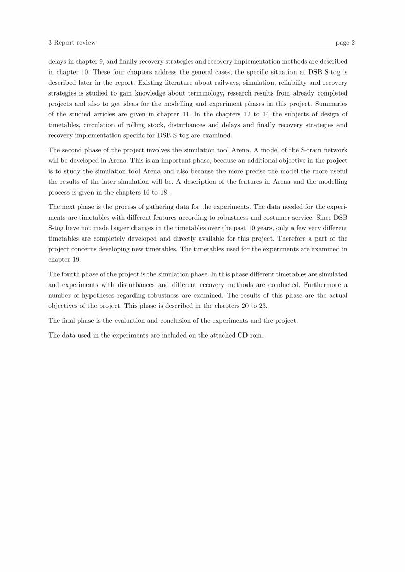
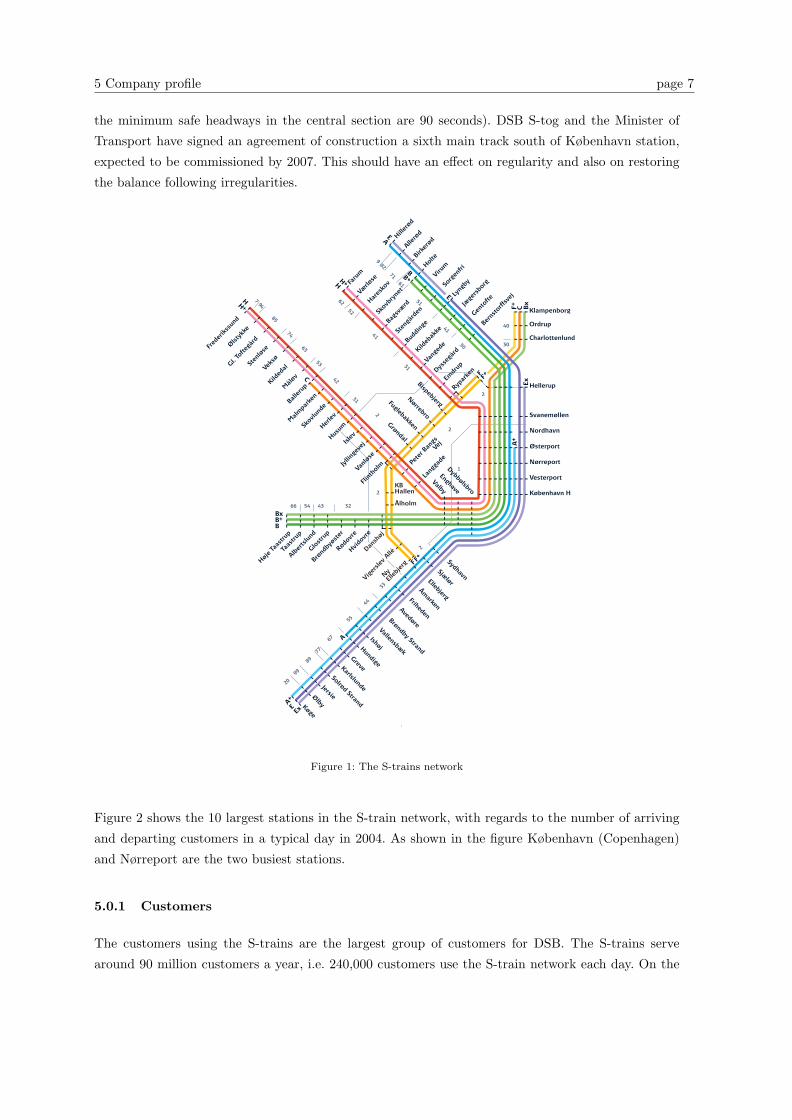
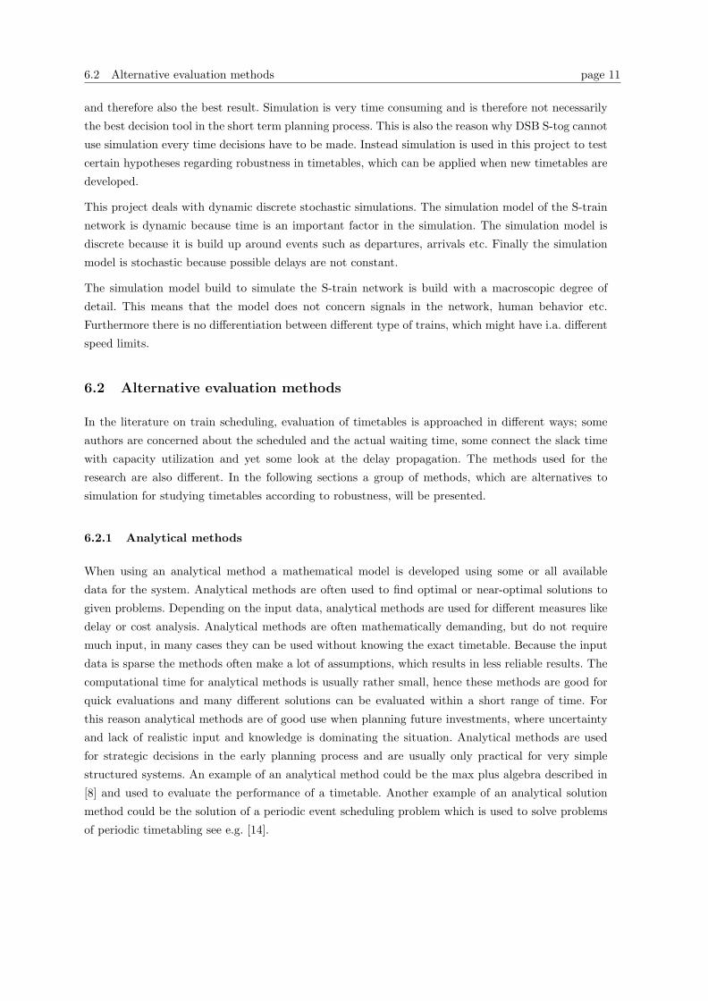
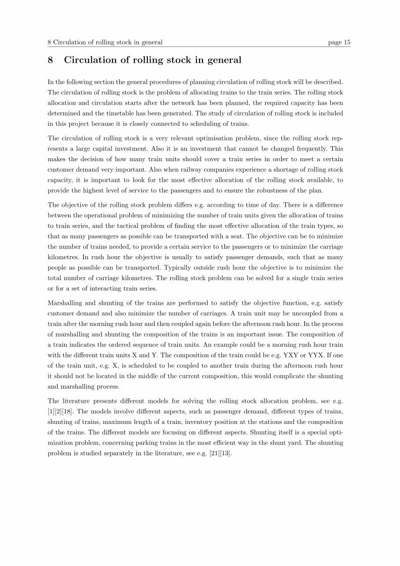
The S-train network consists of 170 km double tracks and 80 stations. The network is constantly
occupied by approximately 80 trains during the day and there are 1100 departures daily. The S-train
network is displayed in Figure 1. The figure shows the stations, the train series and the lines in the
current plan. The numbers in the figure refer to the different zones relating to the cost of travelling.
There are 5 main train series in the S-train network; Køge-Hillerød, Høje Taastrup-Holte, Frederikssund-
Farum, Ballerup-Klampenborg and Ny Ellebjerg-Hellerup. The train series are covered by different
lines, indicated by different colours and the capital letters A, B, C, E, F, and H. For example the train
series between Høje Taastrup and Holte is covered by the green line B. The line B+ is also covering
the train series between Høje Taastrup and Holte but this line is only used during daily hours. This
is the case for all the +-lines. The x-lines are only used during the rush hour in the morning and in
the afternoon. All the lines have a frequency of 20 minutes and are run according to an hourly cyclic
timetable. When more departures are needed to fulfil the demand, extra lines are used to cover the
series. This explains the +-lines and the x-lines. Main lines and extra lines, e.g. B and B+, are run
with 10 minute intervals. The lines F and F+, covering the train series between Ny Ellebjerg and
Hellerup, is called Ringbanen because it runs around the city.
As all trains in the network travel from one end station to another in the train series, the distance
between København (Copenhagen central station) and Svanemøllen defines a bottleneck. Since all
trains (excluding Ringbanen) has to travel through this part of the network and the frequencies on
all lines are 20 minutes there is a limit on the number of trains passing this section. Currently the
headways in the central section are scheduled to be 2 min. and the frequency is 20 minutes, hence
a maximum of 10 train lines can traverse the tracks from København to Svanemøllen (in practice
5 Company profile page 7
the minimum safe headways in the central section are 90 seconds). DSB S-tog and the Minister of
Transport have signed an agreement of construction a sixth main track south of København station,
expected to be commissioned by 2007. This should have an effect on regularity and also on restoring
the balance following irregularities.
66 54 43 32
20
99
89
77
67
55
44
33
2
82
7161
51
41
30
62
52
41
31
94
85
74
63
53
42
31
2
7
9
1
40
30
2
2
2
København H
Sydhavn
Peter
Ban
gsVej
SjælørEllebjerg
Åmarken
FrihedenAvedøre
Brøndby Strand
Vallensbæk
IshøjHundigeGreveKarlslunde
Solrød Strand
JersieØlbyKøge
Berns
torff
svej
Gento
fteJæ
gers
borg
Lyng
bySorg
enfri
VirumHolteBirk
erød
Allerø
dHiller
ød
Rødovre
Brønd
byøst
er
Glost
rup
Alber
tslu
nd
Taas
trup
Høje Ta
astru
p
Vesterport
Nørreport
Nordhavn
Svanemøllen
Hellerup
Charlottenlund
Ordrup
Klampenborg
Emdru
p
Rypar
kenDys
segå
rd
Vange
deKild
ebak
ke
Buddinge
Sten
gård
en
Bagsv
ærd
Skovb
ryne
t
Hares
kov
Værlø
seFaru
m
Bispebjerg
Valby
Enghave
Dybbølsbro
Vanlø
se
Jylli
ngev
ejIsle
vHusumHer
lev
Skovl
unde
Mal
mpar
ken
Balle
rupM
åløv
Kilded
alVeksø
Lang
gade
Sten
løse
Ølst
ykke
Gl. To
ftegå
rd
Hvidovr
e
Østerport
Fred
erik
ssund
Flin
tholm
Nørrebro
FuglebakkenGrøndal
Dansh
øj
KBHallen
Ålholm
Viger
slev
Allé
NyEl
lebje
rg
C
H +
EA
BB +
H
F+
CBxB+B
A+
E
Ex
A
A+E
H +H
F
Ex
FF+
Bx
F+
DSB S-togKøreplan Gælder fra januar 2005
Figure 1: The S-trains network
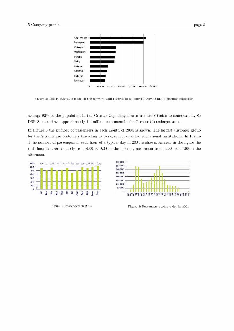
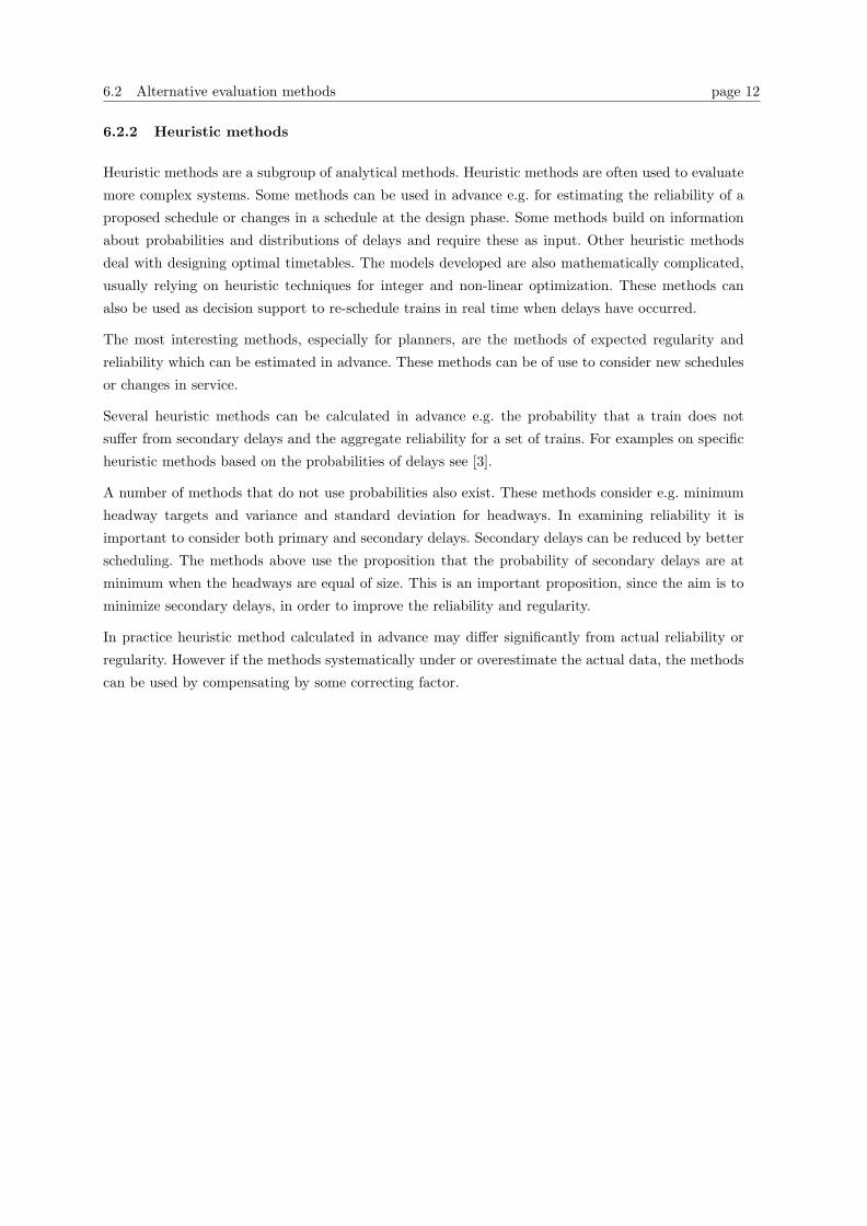
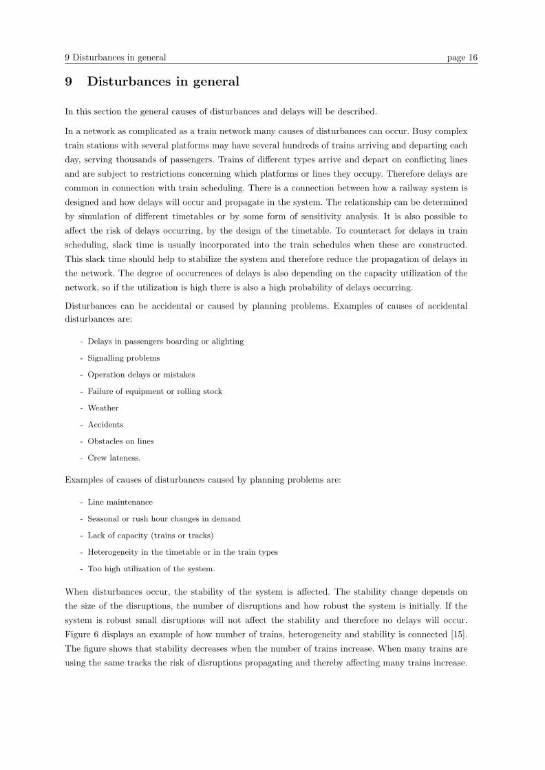
Figure 2 shows the 10 largest stations in the S-train network, with regards to the number of arriving
and departing customers in a typical day in 2004. As shown in the figure København (Copenhagen)
and Nørreport are the two busiest stations.
5.0.1 Customers
The customers using the S-trains are the largest group of customers for DSB. The S-trains serve
around 90 million customers a year, i.e. 240,000 customers use the S-train network each day. On the
5 Company profile page 8
Figure 2: The 10 largest stations in the network with regards to number of arriving and departing passengers
average 92% of the population in the Greater Copenhagen area use the S-trains to some extent. So
DSB S-trains have approximately 1.4 million customers in the Greater Copenhagen area.
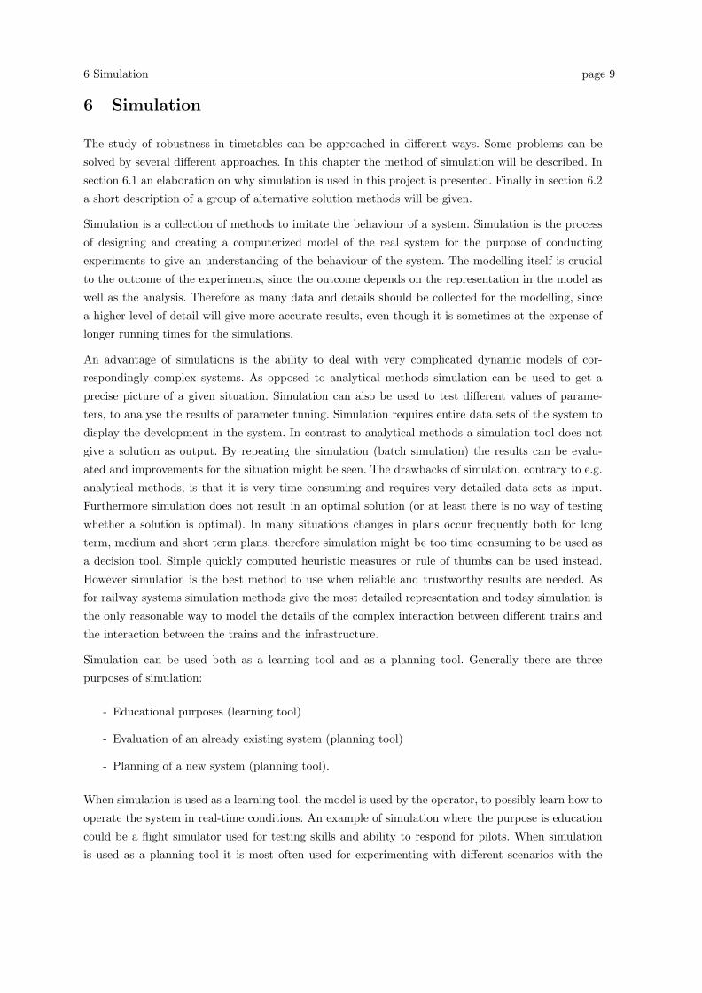
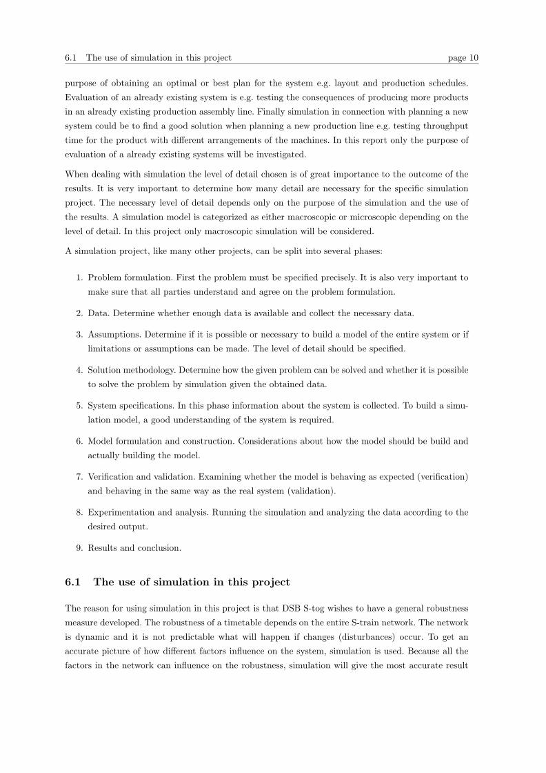
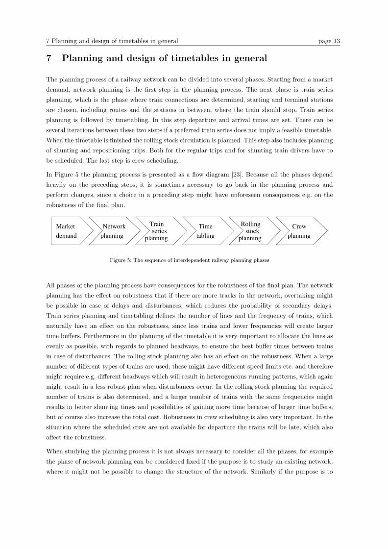
In Figure 3 the number of passengers in each month of 2004 is shown. The largest customer group
for the S-trains are customers travelling to work, school or other educational institutions. In Figure
4 the number of passengers in each hour of a typical day in 2004 is shown. As seen in the figure the
rush hour is approximately from 6:00 to 9:00 in the morning and again from 15:00 to 17:00 in the
afternoon.
Figure 3: Passengers in 2004 Figure 4: Passengers during a day in 2004
6 Simulation page 9
6 Simulation
The study of robustness in timetables can be approached in different ways. Some problems can be
solved by several different approaches. In this chapter the method of simulation will be described. In
section 6.1 an elaboration on why simulation is used in this project is presented. Finally in section 6.2
a short description of a group of alternative solution methods will be given.
Simulation is a collection of methods to imitate the behaviour of a system. Simulation is the process
of designing and creating a computerized model of the real system for the purpose of conducting
experiments to give an understanding of the behaviour of the system. The modelling itself is crucial
to the outcome of the experiments, since the outcome depends on the representation in the model as
well as the analysis. Therefore as many data and details should be collected for the modelling, since
a higher level of detail will give more accurate results, even though it is sometimes at the expense of
longer running times for the simulations.
An advantage of simulations is the ability to deal with very complicated dynamic models of cor-
respondingly complex systems. As opposed to analytical methods simulation can be used to get a
precise picture of a given situation. Simulation can also be used to test different values of parame-
ters, to analyse the results of parameter tuning. Simulation requires entire data sets of the system to
display the development in the system. In contrast to analytical methods a simulation tool does not
give a solution as output. By repeating the simulation (batch simulation) the results can be evalu-
ated and improvements for the situation might be seen. The drawbacks of simulation, contrary to e.g.
analytical methods, is that it is very time consuming and requires very detailed data sets as input.
Furthermore simulation does not result in an optimal solution (or at least there is no way of testing
whether a solution is optimal). In many situations changes in plans occur frequently both for long
term, medium and short term plans, therefore simulation might be too time consuming to be used as
a decision tool. Simple quickly computed heuristic measures or rule of thumbs can be used instead.
However simulation is the best method to use when reliable and trustworthy results are needed. As
for railway systems simulation methods give the most detailed representation and today simulation is
the only reasonable way to model the details of the complex interaction between different trains and
the interaction between the trains and the infrastructure.
Simulation can be used both as a learning tool and as a planning tool. Generally there are three
purposes of simulation:
- Educational purposes (learning tool)
- Evaluation of an already existing system (planning tool)
- Planning of a new system (planning tool).
When simulation is used as a learning tool, the model is used by the operator, to possibly learn how to
operate the system in real-time conditions. An example of simulation where the purpose is education
could be a flight simulator used for testing skills and ability to respond for pilots. When simulation
is used as a planning tool it is most often used for experimenting with different scenarios with the
6.1 The use of simulation in this project page 10
purpose of obtaining an optimal or best plan for the system e.g. layout and production schedules.
Evaluation of an already existing system is e.g. testing the consequences of producing more products
in an already existing production assembly line. Finally simulation in connection with planning a new
system could be to find a good solution when planning a new production line e.g. testing throughput
time for the product with different arrangements of the machines. In this report only the purpose of
evaluation of a already existing systems will be investigated.
When dealing with simulation the level of detail chosen is of great importance to the outcome of the
results. It is very important to determine how many detail are necessary for the specific simulation
project. The necessary level of detail depends only on the purpose of the simulation and the use of
the results. A simulation model is categorized as either macroscopic or microscopic depending on the
level of detail. In this project only macroscopic simulation will be considered.
A simulation project, like many other projects, can be split into several phases:
1. Problem formulation. First the problem must be specified precisely. It is also very important to
make sure that all parties understand and agree on the problem formulation.
2. Data. Determine whether enough data is available and collect the necessary data.
3. Assumptions. Determine if it is possible or necessary to build a model of the entire system or if
limitations or assumptions can be made. The level of detail should be specified.
4. Solution methodology. Determine how the given problem can be solved and whether it is possible
to solve the problem by simulation given the obtained data.
5. System specifications. In this phase information about the system is collected. To build a simu-
lation model, a good understanding of the system is required.
6. Model formulation and construction. Considerations about how the model should be build and
actually building the model.
7. Verification and validation. Examining whether the model is behaving as expected (verification)
and behaving in the same way as the real system (validation).
8. Experimentation and analysis. Running the simulation and analyzing the data according to the
desired output.
9. Results and conclusion.
6.1 The use of simulation in this project
The reason for using simulation in this project is that DSB S-tog wishes to have a general robustness
measure developed. The robustness of a timetable depends on the entire S-train network. The network
is dynamic and it is not predictable what will happen if changes (disturbances) occur. To get an
accurate picture of how different factors influence on the system, simulation is used. Because all the
factors in the network can influence on the robustness, simulation will give the most accurate result
6.2 Alternative evaluation methods page 11
and therefore also the best result. Simulation is very time consuming and is therefore not necessarily
the best decision tool in the short term planning process. This is also the reason why DSB S-tog cannot
use simulation every time decisions have to be made. Instead simulation is used in this project to test
certain hypotheses regarding robustness in timetables, which can be applied when new timetables are
developed.
This project deals with dynamic discrete stochastic simulations. The simulation model of the S-train
network is dynamic because time is an important factor in the simulation. The simulation model is
discrete because it is build up around events such as departures, arrivals etc. Finally the simulation
model is stochastic because possible delays are not constant.
The simulation model build to simulate the S-train network is build with a macroscopic degree of
detail. This means that the model does not concern signals in the network, human behavior etc.
Furthermore there is no differentiation between different type of trains, which might have i.a. different
speed limits.
6.2 Alternative evaluation methods
In the literature on train scheduling, evaluation of timetables is approached in different ways; some
authors are concerned about the scheduled and the actual waiting time, some connect the slack time
with capacity utilization and yet some look at the delay propagation. The methods used for the
research are also different. In the following sections a group of methods, which are alternatives to
simulation for studying timetables according to robustness, will be presented.
6.2.1 Analytical methods
When using an analytical method a mathematical model is developed using some or all available
data for the system. Analytical methods are often used to find optimal or near-optimal solutions to
given problems. Depending on the input data, analytical methods are used for different measures like
delay or cost analysis. Analytical methods are often mathematically demanding, but do not require
much input, in many cases they can be used without knowing the exact timetable. Because the input
data is sparse the methods often make a lot of assumptions, which results in less reliable results. The
computational time for analytical methods is usually rather small, hence these methods are good for
quick evaluations and many different solutions can be evaluated within a short range of time. For
this reason analytical methods are of good use when planning future investments, where uncertainty
and lack of realistic input and knowledge is dominating the situation. Analytical methods are used
for strategic decisions in the early planning process and are usually only practical for very simple
structured systems. An example of an analytical method could be the max plus algebra described in
[8] and used to evaluate the performance of a timetable. Another example of an analytical solution
method could be the solution of a periodic event scheduling problem which is used to solve problems
of periodic timetabling see e.g. [14].
6.2 Alternative evaluation methods page 12
6.2.2 Heuristic methods
Heuristic methods are a subgroup of analytical methods. Heuristic methods are often used to evaluate
more complex systems. Some methods can be used in advance e.g. for estimating the reliability of a
proposed schedule or changes in a schedule at the design phase. Some methods build on information
about probabilities and distributions of delays and require these as input. Other heuristic methods
deal with designing optimal timetables. The models developed are also mathematically complicated,
usually relying on heuristic techniques for integer and non-linear optimization. These methods can
also be used as decision support to re-schedule trains in real time when delays have occurred.
The most interesting methods, especially for planners, are the methods of expected regularity and
reliability which can be estimated in advance. These methods can be of use to consider new schedules
or changes in service.
Several heuristic methods can be calculated in advance e.g. the probability that a train does not
suffer from secondary delays and the aggregate reliability for a set of trains. For examples on specific
heuristic methods based on the probabilities of delays see [3].
A number of methods that do not use probabilities also exist. These methods consider e.g. minimum
headway targets and variance and standard deviation for headways. In examining reliability it is
important to consider both primary and secondary delays. Secondary delays can be reduced by better
scheduling. The methods above use the proposition that the probability of secondary delays are at
minimum when the headways are equal of size. This is an important proposition, since the aim is to
minimize secondary delays, in order to improve the reliability and regularity.
In practice heuristic method calculated in advance may differ significantly from actual reliability or
regularity. However if the methods systematically under or overestimate the actual data, the methods
can be used by compensating by some correcting factor.
7 Planning and design of timetables in general page 13
7 Planning and design of timetables in general
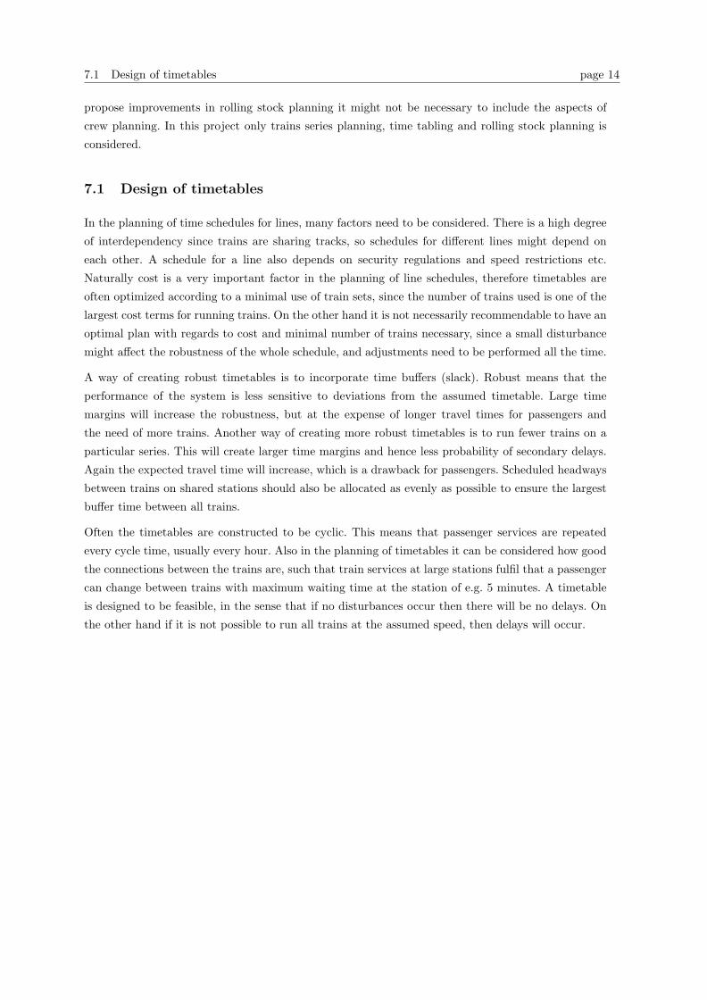
The planning process of a railway network can be divided into several phases. Starting from a market
demand, network planning is the first step in the planning process. The next phase is train series
planning, which is the phase where train connections are determined, starting and terminal stations
are chosen, including routes and the stations in between, where the train should stop. Train series
planning is followed by timetabling. In this step departure and arrival times are set. There can be
several iterations between these two steps if a preferred train series does not imply a feasible timetable.
When the timetable is finished the rolling stock circulation is planned. This step also includes planning
of shunting and repositioning trips. Both for the regular trips and for shunting train drivers have to
be scheduled. The last step is crew scheduling.
In Figure 5 the planning process is presented as a flow diagram [23]. Because all the phases depend
heavily on the preceding steps, it is sometimes necessary to go back in the planning process and
perform changes, since a choice in a preceding step might have unforeseen consequences e.g. on the
robustness of the final plan.
Market planningNetwork
demandstock
Time series
tablingplanning
Train
planning
Rolling
planningCrew
Figure 5: The sequence of interdependent railway planning phases
All phases of the planning process have consequences for the robustness of the final plan. The network
planning has the effect on robustness that if there are more tracks in the network, overtaking might
be possible in case of delays and disturbances, which reduces the probability of secondary delays.
Train series planning and timetabling defines the number of lines and the frequency of trains, which
naturally have an effect on the robustness, since less trains and lower frequencies will create larger
time buffers. Furthermore in the planning of the timetable it is very important to allocate the lines as
evenly as possible, with regards to planned headways, to ensure the best buffer times between trains
in case of disturbances. The rolling stock planning also has an effect on the robustness. When a large
number of different types of trains are used, these might have different speed limits etc. and therefore
might require e.g. different headways which will result in heterogeneous running patterns, which again
might result in a less robust plan when disturbances occur. In the rolling stock planning the required
number of trains is also determined, and a larger number of trains with the same frequencies might
results in better shunting times and possibilities of gaining more time because of larger time buffers,
but of course also increase the total cost. Robustness in crew scheduling is also very important. In the
situation where the scheduled crew are not available for departure the trains will be late, which also
affect the robustness.
When studying the planning process it is not always necessary to consider all the phases, for example
the phase of network planning can be considered fixed if the purpose is to study an existing network,
where it might not be possible to change the structure of the network. Similarly if the purpose is to
7.1 Design of timetables page 14
propose improvements in rolling stock planning it might not be necessary to include the aspects of
crew planning. In this project only trains series planning, time tabling and rolling stock planning is
considered.
7.1 Design of timetables
In the planning of time schedules for lines, many factors need to be considered. There is a high degree
of interdependency since trains are sharing tracks, so schedules for different lines might depend on
each other. A schedule for a line also depends on security regulations and speed restrictions etc.
Naturally cost is a very important factor in the planning of line schedules, therefore timetables are
often optimized according to a minimal use of train sets, since the number of trains used is one of the
largest cost terms for running trains. On the other hand it is not necessarily recommendable to have an
optimal plan with regards to cost and minimal number of trains necessary, since a small disturbance
might affect the robustness of the whole schedule, and adjustments need to be performed all the time.
A way of creating robust timetables is to incorporate time buffers (slack). Robust means that the
performance of the system is less sensitive to deviations from the assumed timetable. Large time
margins will increase the robustness, but at the expense of longer travel times for passengers and
the need of more trains. Another way of creating more robust timetables is to run fewer trains on a
particular series. This will create larger time margins and hence less probability of secondary delays.
Again the expected travel time will increase, which is a drawback for passengers. Scheduled headways
between trains on shared stations should also be allocated as evenly as possible to ensure the largest
buffer time between all trains.
Often the timetables are constructed to be cyclic. This means that passenger services are repeated
every cycle time, usually every hour. Also in the planning of timetables it can be considered how good
the connections between the trains are, such that train services at large stations fulfil that a passenger
can change between trains with maximum waiting time at the station of e.g. 5 minutes. A timetable
is designed to be feasible, in the sense that if no disturbances occur then there will be no delays. On
the other hand if it is not possible to run all trains at the assumed speed, then delays will occur.
8 Circulation of rolling stock in general page 15
8 Circulation of rolling stock in general
In the following section the general procedures of planning circulation of rolling stock will be described.
The circulation of rolling stock is the problem of allocating trains to the train series. The rolling stock
allocation and circulation starts after the network has been planned, the required capacity has been
determined and the timetable has been generated. The study of circulation of rolling stock is included
in this project because it is closely connected to scheduling of trains.
The circulation of rolling stock is a very relevant optimisation problem, since the rolling stock rep-
resents a large capital investment. Also it is an investment that cannot be changed frequently. This
makes the decision of how many train units should cover a train series in order to meet a certain
customer demand very important. Also when railway companies experience a shortage of rolling stock
capacity, it is important to look for the most effective allocation of the rolling stock available, to
provide the highest level of service to the passengers and to ensure the robustness of the plan.
The objective of the rolling stock problem differs e.g. according to time of day. There is a difference
between the operational problem of minimizing the number of train units given the allocation of trains
to train series, and the tactical problem of finding the most effective allocation of the train types, so
that as many passengers as possible can be transported with a seat. The objective can be to minimize
the number of trains needed, to provide a certain service to the passengers or to minimize the carriage
kilometres. In rush hour the objective is usually to satisfy passenger demands, such that as many
people as possible can be transported. Typically outside rush hour the objective is to minimize the
total number of carriage kilometres. The rolling stock problem can be solved for a single train series
or for a set of interacting train series.
Marshalling and shunting of the trains are performed to satisfy the objective function, e.g. satisfy
customer demand and also minimize the number of carriages. A train unit may be uncoupled from a
train after the morning rush hour and then coupled again before the afternoon rush hour. In the process
of marshalling and shunting the composition of the trains is an important issue. The composition of
a train indicates the ordered sequence of train units. An example could be a morning rush hour train
with the different train units X and Y. The composition of the train could be e.g. YXY or YYX. If one
of the train unit, e.g. X, is scheduled to be coupled to another train during the afternoon rush hour
it should not be located in the middle of the current composition, this would complicate the shunting
and marshalling process.
The literature presents different models for solving the rolling stock allocation problem, see e.g.
[1][2][18]. The models involve different aspects, such as passenger demand, different types of trains,
shunting of trains, maximum length of a train, inventory position at the stations and the composition
of the trains. The different models are focusing on different aspects. Shunting itself is a special opti-
mization problem, concerning parking trains in the most efficient way in the shunt yard. The shunting
problem is studied separately in the literature, see e.g. [21][13].
9 Disturbances in general page 16
9 Disturbances in general
In this section the general causes of disturbances and delays will be described.
In a network as complicated as a train network many causes of disturbances can occur. Busy complex
train stations with several platforms may have several hundreds of trains arriving and departing each
day, serving thousands of passengers. Trains of different types arrive and depart on conflicting lines
and are subject to restrictions concerning which platforms or lines they occupy. Therefore delays are
common in connection with train scheduling. There is a connection between how a railway system is
designed and how delays will occur and propagate in the system. The relationship can be determined
by simulation of different timetables or by some form of sensitivity analysis. It is also possible to
affect the risk of delays occurring, by the design of the timetable. To counteract for delays in train
scheduling, slack time is usually incorporated into the train schedules when these are constructed.
This slack time should help to stabilize the system and therefore reduce the propagation of delays in
the network. The degree of occurrences of delays is also depending on the capacity utilization of the
network, so if the utilization is high there is also a high probability of delays occurring.
Disturbances can be accidental or caused by planning problems. Examples of causes of accidentaldisturbances are:
- Delays in passengers boarding or alighting
- Signalling problems
- Operation delays or mistakes
- Failure of equipment or rolling stock
- Weather
- Accidents
- Obstacles on lines
- Crew lateness.
Examples of causes of disturbances caused by planning problems are:
- Line maintenance
- Seasonal or rush hour changes in demand
- Lack of capacity (trains or tracks)
- Heterogeneity in the timetable or in the train types
- Too high utilization of the system.
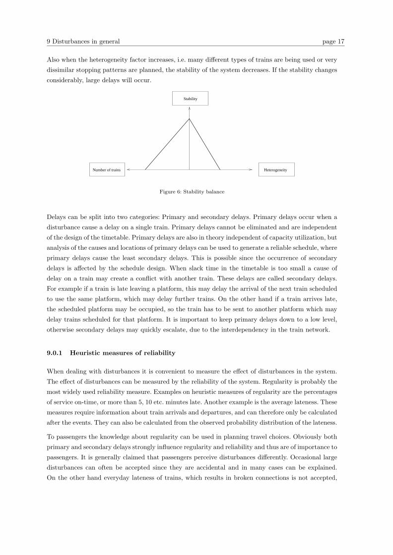
When disturbances occur, the stability of the system is affected. The stability change depends on
the size of the disruptions, the number of disruptions and how robust the system is initially. If the
system is robust small disruptions will not affect the stability and therefore no delays will occur.
Figure 6 displays an example of how number of trains, heterogeneity and stability is connected [15].
The figure shows that stability decreases when the number of trains increase. When many trains are
using the same tracks the risk of disruptions propagating and thereby affecting many trains increase.
9 Disturbances in general page 17
Also when the heterogeneity factor increases, i.e. many different types of trains are being used or very
dissimilar stopping patterns are planned, the stability of the system decreases. If the stability changes
considerably, large delays will occur.
Stability
Number of trains Heterogeneity
Figure 6: Stability balance
Delays can be split into two categories: Primary and secondary delays. Primary delays occur when a
disturbance cause a delay on a single train. Primary delays cannot be eliminated and are independent
of the design of the timetable. Primary delays are also in theory independent of capacity utilization, but
analysis of the causes and locations of primary delays can be used to generate a reliable schedule, where
primary delays cause the least secondary delays. This is possible since the occurrence of secondary
delays is affected by the schedule design. When slack time in the timetable is too small a cause of
delay on a train may create a conflict with another train. These delays are called secondary delays.
For example if a train is late leaving a platform, this may delay the arrival of the next train scheduled
to use the same platform, which may delay further trains. On the other hand if a train arrives late,
the scheduled platform may be occupied, so the train has to be sent to another platform which may
delay trains scheduled for that platform. It is important to keep primary delays down to a low level,
otherwise secondary delays may quickly escalate, due to the interdependency in the train network.
9.0.1 Heuristic measures of reliability
When dealing with disturbances it is convenient to measure the effect of disturbances in the system.
The effect of disturbances can be measured by the reliability of the system. Regularity is probably the
most widely used reliability measure. Examples on heuristic measures of regularity are the percentages
of service on-time, or more than 5, 10 etc. minutes late. Another example is the average lateness. These
measures require information about train arrivals and departures, and can therefore only be calculated
after the events. They can also be calculated from the observed probability distribution of the lateness.
To passengers the knowledge about regularity can be used in planning travel choices. Obviously both
primary and secondary delays strongly influence regularity and reliability and thus are of importance to
passengers. It is generally claimed that passengers perceive disturbances differently. Occasional large
disturbances can often be accepted since they are accidental and in many cases can be explained.
On the other hand everyday lateness of trains, which results in broken connections is not accepted,
9 Disturbances in general page 18
therefore these minor disturbances should be avoided. Another reason for avoiding too many small
disturbances is that these may easily cause large delays over time. An important issue in connection
with reliability is the door-to-door travel time, which means that it is not only the regularity of one
train that is important, the connections to other trains are just as important, because it is the entire
travel time the passengers are concerned about. If the connections are trustworthy it is easier for the
passengers to plan their transport. To operators and marketing heuristic measures of reliability can be
used to plan, manage, control and improve services. To the top management the measures are needful
to check if operators deliver what they promise in terms of quality of service or contracted goals.
10 Recovery strategies and methods in general page 19
10 Recovery strategies and methods in general
As described earlier, many different types of disturbances may occur in the daily operation of railways.
These disturbances can be dealt with in different ways; by re-establishing the original plan, by re-
scheduling or by regaining regular headways. The three strategies will be examined in this chapter.
The distinction between strategies is inspired from the different recovery strategies described in the
literature see e.g. [10][7]. The different recovery strategies represent several recovery methods such as
cancelling trains, replacing late trains or reducing minimum dwell times. An examination of different
implementations of recovery methods is also made in this chapter.
10.1 Recovery strategies
Management by re-establishing the original plan
In this strategy the traffic controllers try to solve the problems by using the time margins (slack) build
into the timetable. Connections between different trains may be broken, trains may be late, platforms
may be changed, running times and dwell times may be reduced, but generally the plan remains intact.
This strategy is usually used to deal with minor disturbances, since otherwise it may take too long to
re-establish the original plan. Management of minor disturbances is usually predictable. There might
be rules for how long a train may wait at stations for connections or rules to change order of trains if
only one train is late. Two examples of how re-establishing can be used are given in the following.
When trains are late at arrival, reducing the dwell times can help trains get back on time. Suppose
a train has a scheduled dwell time of 6 minutes and a minimum required dwell time of 3 minutes. If
it arrives 4 minutes late, it can be ready to depart after 3 minutes, hence only 1 minute late instead
of 4 minutes. On the other hand if the minimum dwell time is 1 minute, it is ready to depart after 1
minute, but of course it is not allowed to depart before the scheduled time, hence the train can leave
on time after 2 minutes, and thereby the delay has been eliminated.
If trains arrive later than scheduled their assigned platform may be occupied by later trains. In this
case the train could be held until the assigned platform becomes free. On the other hand it could
also be send to another platform if one becomes free sooner. Similarly if a train departs late, the next
train scheduled for the same platform can either wait until the platform becomes available, or go to
another platform if one becomes free sooner. It should be noted though that these on-the-day changes
in platforms may cause further secondary delays to the following trains if not done carefully, which
should be considered before allowing changes. Experiments have shown that allowing the change of
platform reduces secondary delays [4]. The strategy depends on how heavily congested the system is.
If trains run on a very tight schedule it might not be such a good idea, to allow changes in platform,
since this will disrupt a large number of trains. On the other hand if the schedules contain larger
headways it might reduce delays considerably. The strategy also depends on whether all platforms
are feasible for all train types. Furthermore there might be some restrictions due to the layout of the
network, which might prevent the strategy from being possible. Regarding passenger satisfaction, it
should also be considered whether it is convenient to get from one platform to the others.
10.2 Implementation of recovery methods page 20
Management by re-scheduling
In this recovery strategy trains or lines may by re-routed or cancelled. Essentially a new plan is made
and the logistical plan is disrupted. The goal in the end is to re-establish the original plan but this
may take several hours, or it might not even be possible within the same day. This strategy is used in
operations when major incidents cause delays e.g. accidents or rolling stock failure. There might be
rules on which train lines to cancel in case of disturbance or which lines to re-route. Even if certain
rules exist for management of large disturbances, the outcome still depends very much on the exact
circumstances and on the choices made by the operator responsible for traffic control.
Management by regaining regular headways
A third recovery strategy is to regain regular headways as quick as possible. After a disruption the
affected trains may be clustered. Instead of waiting for the scheduled departure time for every train
they are set off as fast at possible with the smallest possible headways. The idea is to get as many
trains rolling as possible and maximizing capacity utilization. This recovery strategy is mostly used in
urban rail network where the trains are scheduled to run within small intervals e.g. metro systems. On
very busy stations the exact minute of departure is not of most importance because the frequencies
of train departures are very large. If e.g. trains are running between two stations with an interval of
3 minutes it seldom matters to passengers exactly what train is reached. In longer term when the
disruption is stabilized the trains are re-scheduled to the original plan.
10.2 Implementation of recovery methods
In this section two different ways of implementing recovery methods are examined. The first imple-
mentation method is referred to as an ’expert system’, because a set of rules are used to recover
when disruptions occur. The rules are derived from operational experience or the acquired skills of the
control centerer staff. These rules can be implemented in a computer, written down in a rule book or
just be in memory of the operators. Whenever the rules are developed this can be a quick method of
determining a recovery solution, but the solution is not necessarily the best possible, and therefore it
is important to evaluate the results of a recovery and the rules should be updated continuously.
The other implementation method is based on a mathematical model with an objective function and
a search procedure. The objective function must optimize the recovery and the search procedure
must be used to find the set of operation instructions that optimizes the objective function. This
implementation method is often not very fast but gives an optimal solution. Furthermore it is not
always straight forward to develop the objective function, to find an appropriate search procedure, or
to model the appropriate constraints.
The difference of computer decided or train operator decided recovery is also of importance. When
smaller disturbances are to be eliminated the decisions are often made by a computer system and for
bigger disturbances train operators make the final decisions. The two implementation methods can
also be combined.
11 Literature review page 21
11 Literature review
In the literature several related problems concerning planning and scheduling of timetables is treated.
In this chapter a number of articles on the subject is reviewed. First some articles on simulation are
reviewed. These are of great interest because simulation is the subject of this project. Then a number
of articles describing reliability and measures of reliability are addressed. The articles are relevant in
connection with measuring robustness of a timetable, since reliability can be used as a measure of
robustness. Then a few articles about recovery methods are presented. Recovery is of interest in this
connection because it is important to investigate how a timetable react when disturbances occur, and
also to examine how easily an affected timetables can be re-established. Finally a couple of articles
concerning allocation of rolling stock and shunting are included, because these article are proven
very useful in gaining knowledge about terminology and understanding basic concepts within railway
planning and timetable scheduling.
11.1 Literature on simulation
The use of simulation in the planning of the Dutch railway services
Hoogheimstra and Teunisse [10] describe their research on robustness in timetables in the Dutch
railway network. The authors present their considerations about planning of the infrastructure and
timetables. They also state the importance of reliability and punctuality. A program called DONS
(Designer Of Network Schedules) is used to generate timetables. The goal of the paper is to determine
if construction of timetables can be refined to increase the robustness of the operation. To attain this
goal a DONS-simulator is developed. The simulation tool enables the authors to study the effect of
small disturbances on the punctuality of trains in the entire network. The simulator will also be used
to evaluate how investments in infrastructure effects punctuality in later research. This paper does
not present the final results of the research. The paper only describes the building and testing process
of a prototype of the DONS-simulator. In the following article “Simone: Large scale train network
simulations” [16] the final simulation tool is described.
Simone: Large scale train network simulations
Middelkoop and Bouwman [16] describes the architecture and features of the simulation program
Simone (Simulation Model Network). Simone is a simulation environment developed with the purpose
of determining the robustness of a timetable and the stability of a railway network, and thereby
improve the quality and stability of the timetables from a set of different criteria. It does this by
determining bottlenecks in the network, by examining the number of delayed departures for all the
stations in the network. Simone can also be used for analyzing delays and exploring causes and effects
of delays for different layouts of railway infrastructures and timetables. Simone can simulate an entire
railway network, compared to other models, studied in connection with the literature review in this
report, which are limited to a smaller set of elements e.g. one train line or a small number of stations.
11.1 Literature on simulation page 22
The article describes the Dutch rail network, for which Simone has been designed. Netherlands rail
network consists of almost 600 stations (including junctions) and about 2750 kilometer tracks. Simone
is used to compare the quality of different timetables. Quality in timetables depends on network
properties such as correspondences between trains and use of shared capacity.
Central in Simone is the timetable, which drives the activities. When there are no disturbances all
trains run according to schedule. When disturbances occur Simone inspects the different types of delays
(primary and secondary) and the user gets extensive information on the delays and delay propagation
in a specific simulation. Simone also provides other information and statistics on the states of the
trains and stations in the model. This makes it useful for comparing the robustness and punctuality
of different timetables.
The article also describes the architecture and functionalities of Simone in more details and shows some
graphical representations of train networks. Also a case study for a specific station in the Netherlands
is given in the articles. The case study shows some of the functions in the program.
The authors describe how Simone has been used on several different studies already with good results
and that it proves to be a good research tool. It provides insight on the performance of different
timetable and infrastructure combinations. An advantage is the possibility of simulation an entire
railway network.
Simulatorsystem inom tagtrafikstyring, en kundskapsdokumentation
English title: A train traffic operation and planning simulator within railways
In the report [20] Sandblad et al. describe various concepts within simulation of train traffic for use
in both planning and training. The article is an introduction to simulation in general.
They describe the development of a new simulator system which can contribute to improved methods
for train traffic planning, experiments for developing new systems and training of operators.
The report explains the purpose of using simulation in train traffic planning in general. It also explains
the difference between simulation as a planning tool and as a learning tool. There is also a thorough
description of other purposes of simulation e.g. understanding the behaviour of the system, as a base
for difficult decisions, or for controlling the system.
In addition the report describes the different phases in the planning and implementation of a simula-
tion project. These include problem specification, construction of the model, validation of the model,
programming, verification of the program, planning the experiments, realization of experiments, eval-
uation of results and conclusion.
The article includes many descriptions of concepts. Some of these concepts are symbolic models (which
build on mathematical equations) as opposed to iconic models. Stochastic models contra deterministic
models is also explained. Finally modelling time, continuous simulation vs. event simulation (discrete
simulation), real-time simulation and batch simulation are described.
11.2 Literature on reliability page 23
11.1.1 Comparison of the literature on simulation
The first two articles described in the previous section are both dealing with simulation used as
a planning tool in the Dutch railway services. The first article describes the early phases in the
development of the simulation tool and the second one the actual simulation tool that has been
implemented. The tool has not been completed at the time of the publication, but it has not been
possible to find more recent articles on the subject. Both articles are interesting because the scopes
are the same as for this project, that is developing a simulation model which can be used to analyze
robustness, delay propagation etc. for a railway network. The simulation model in the articles are
developed for the entire Dutch railway network, which is much larger than the network dealt with in
this project. The articles have been very useful in gaining knowledge about simulation of railways.
The third article is an overview of concepts and explains general terms within the field of simulation,
but does not go into further details about modelling, limitations etc. It also describes the general phases
in a simulation project. It does not include any problem cases or evaluation of specific simulation tools.
Therefore it is used as a basic article to get an understanding of the idea of simulation in general.
11.2 Literature on reliability
Ex ante heuristic measures of schedule reliability
In the article [3] Carey describes different heuristic measures of stability. The reason for using these
measures is that analytical methods are practical only for simple system, and simulation methods are
very time consuming, so in practice the most widely used measures are heuristic.
The author choose to focus on measures which can be used in advance for example in the design phase
or to estimate the reliability of a proposed schedule. In practice the percentage of services which are
on time, and the percentage which is more than 5 or 10 minutes late, is often used as a measure
of reliability. These percentages are obtained from the frequency of the distribution of the lateness,
therefore they cannot be used as a measure in advance. It should be noted that even though the
measures in the article are meant to be used in advance some past information is needed to determine
the distribution of the occurrence of delays.
In practice most train conflicts only involve two consecutive trains, so to minimize secondary delays
slack time is usually build into the schedule. Initially the author states a measure of reliability which
assumes that no secondary delays occur, except secondary delays caused by immediately proceeding
trains. This measure is based on the probability of the occurrence of secondary delays, and it is a
measure of the probability that a train keeps within its headway. The measure is also used as a base
to formulate another measure which take all kinds of secondary delays into account.
The author also proposes measures of reliability of an entire schedule. These measures are based on the
mean of the individual train reliabilities. As a second type of measures the author proposes a number
of measures which build on the expected size of the secondary delays, instead of on the probability
of occurrence of secondary delays. Again there is a measure for the expected secondary delays on a
11.2 Literature on reliability page 24
single train, and also a measure of reliability for a whole schedule. Both cases of measures of reliability
are expected to be reasonably good when the stations in the system are not very congested. If heavily
congested the measure based on the expected size of the secondary delays is likely to be best since it
takes into account what happens when trains are delayed more than their scheduled headways. Also
the definition of reliability implies that the reliability always increase with headways. Finally making
headways more equal for all trains, reduce the probability of secondary delays.
Furthermore the author states some heuristic measures of reliability which do not use probabilities.
These measures are not based on information on the previous occurrence of delays. There are several
reasons for preferring these measures over the probabilistic ones e.g. what matters to the decision
maker is not past delays, but future delays. All of these measures are based on the number, size and
spread of minimum headways.
Finally the author plans to test the different measures by comparing the results with results obtained
by using stochastic simulation.
Testing schedule performance and reliability for train stations
In this article [4] Carey and Carville develop a number of experiments with a simulation model to
predict the probability distribution of secondary delays at stations. The purpose is to create a method
that can be used to test and compare reliability of different proposed schedules or schedule changes.
The authors state that all methods developed so far are deterministic models, meaning that the
methods do not indicate how the created schedule will perform when faced with delays. Delays are
common in connection with train scheduling due to e.g. delays in passengers boarding or alighting.
These primary delays cannot be eliminated. Therefore the authors are concerned with developing a
method for describing the behaviour of a train schedule when faced with typical primary delays. This
can be used to find a reliable schedule where primary delays cause the least secondary delays.
The authors describe a number of different experiments. First four experiments are described where
delays are drawn from a uniform distribution and then the same four experiments are presented where
the delays are drawn from a beta distribution. In the first experiments they simulate how secondary
delays vary as the range of primary delays increase and decrease, while holding the number of trains
with primary delays fixed. In the second type of experiments the authors simulate how secondary
delays vary as the percentage of trains having primary delays vary.
In the first experiment the authors investigate the distribution of secondary delays and total number
of delays. They display a number of curves that illustrate the behaviour of percentage of delayed trains
as a function of the minutes of delays. They also calculate the mean of the delays occurring and state
the confidence intervals. They find that the distribution of the means is approximately normal.
In the second experiment they investigate punctuality improvements at a station. One of the experi-
ments is how it affects the punctuality if trains that are late are allowed to depart after a minimum
required dwell time. This turns out to have a great positive effect on punctuality. Also the departure
delays can be reduced compared to the arrival delays.

11.2 Literature on reliability page 25
In the third experiment it is examined how secondary delays vary with the size of the primary delays.
It is shown that secondary delays increase as the maximum primary delays increase.
The fourth experiment research the effect of allowing platform changes on the day. It is noted that
on-the-day changes in platform may cause yet further secondary delays. On the contrary it turns
out that allowing platform changes in response to on-the-day lateness cause a dramatic reduction in
secondary delays.
The remaining experiments in the article research schedule performance when primary delays belong
to a beta distribution. The reason for this is that the probability distribution function of the beta
distribution has a skewed bell shape, with a longer tail of lateness than earliness, which describes real
data from delays in schedules better in practice, than the uniform distribution.
Again experiments with the distribution of secondary delays are performed. These experiments show
how the numbers of primary delays affect the number and size of secondary delays.
There is also an experiment on how secondary delays vary with the percentage of trains subject to
primary delays. It displays that the percentage of trains with secondary delays is almost a linear
function of the percentage of trains with primary delays.
The last experiment deals with the effect of allowing on-the-day platform changes. As for the exper-
iments with the uniform distribution this turns out to have a large positive effect on reducing the
secondary delays.
The simulations in this article can be used for many purposes. First from the distributions of delays the
measures of punctuality can be read directly. The simulations are also useful for identifying reliability
problems and bottlenecks in the system. This can be done by breaking down the delay distributions
for each train service, station, platform, line, train type etc. The simulation model can also be used
to estimate the effect on punctuality of proposed changes in infrastructure.
We find the article very relevant in this context because the purpose of the simulation resembles the
objective of this project. The experiments and results are also very interesting.
Reliability and heterogeneity of railway services
Vromans, Dekker and Kroon [23] present the concepts of reliability in connection with public railway
systems. Reliability is a key factor in transportation to preserve a high customer service level. In railway
services there are many possible causes for disturbances and therefore also many causes for delays to
spread in the system. One way of increasing reliability is to reduce the propagation of delays due to the
interdependence between trains. The shared use of infrastructure by different railway services, different
trains with different speeds and destinations is assumed to be the main reason for the propagation of
delays throughout the network. In the article the authors try to overcome the problem by creating
more homogeneous timetables, and thereby reduce the running time differences per track section.
The article aims at developing timetables which both absorb primary delays fast and cause as few
secondary delays as possible.
11.2 Literature on reliability page 26
The line plan and the timetable determine the heterogeneity of the railway system. In the article
heterogeneity is measured as the average headway at a location along the line or between trains. Reli-
ability in general is most often measured by the percentage of punctuality. This measure is calculated
as the percentage of trains arriving within a certain number of minutes from the scheduled arrival
time.
Railway traffic is considered to be homogeneous if all trains have similar characteristics, especially the
same average speed. If there are large differences in the timetable characteristics of the trains using
the same track then the railway traffic is called heterogeneous. Heterogeneity usually leads to small
headways, which may increase delay propagation in the system. The authors propose a number of
possibilities for homogenization of a railway system: Reducing speed for fast trains, Speeding up slow
trains, equalizing the number of stops etc.
The article presents both a theoretical and a practical case. In the cases the current heterogeneous
situation is compared to an alternative homogeneous situation, where the lines and number of stops are
homogenized as much as possible. The authors use simulation to analyze and evaluate the alternative
timetables. It turns out for both cases that in the homogeneous situation the reliability increases
significantly, meaning that the number of primary and secondary delays decrease, and hence the new
timetables should be more reliable. The authors conclude that other consequences of homogenization
should also be taken into concern e.g. lower customer service and flexibility. The article does not
consider these consequences.
The article is very relevant in relation to robustness, since the measures mentioned can be used to
determine robustness. Furthermore homogeneity in headways turns out to have a significant impact on
robustness which is an important result. The results from the article have been used as an inspiration
for some of the hypotheses tested in this project.
Train service reliability. A survey of methods for deriving relationships for train delays
Mattsson [15] presents a report where the possibility of deriving causal relationships for train delays
are described. Several approaches for the study of primary and secondary delays are reviewed in the
report. The focus is on secondary delays and especially on how the amount of secondary delays can be
related to the amount of primary delays and the capacity utilization. First the author presents some
theories on calculating delay. The author connect the theories about delays to capacity. Obviously a
timetable becomes more robust if it contains slack or buffer time. To increase the buffer time in a
timetable is the same as to reduce the capacity. The discussion about delays therefore involves the
discussion about capacity utilization. If there is lack of capacity the risk for disturbances increases.
The article presents three methods for deriving relationships for train delays; analytical methods,
statistical analysis and simulation approaches. In every subject the author summarize the results from
earlier research of other people. This article is mostly a literature study on the subject. The conclusion
is that the analytical methods and statistical analysis are mathematical demanding and not very
thorough, but they do not require as much input data and computational time as the simulation
methods. When using the first two methods the timetable does not have to be completely developed.

11.3 Literature on timetables page 27
This makes the methods good strategic decision tools in the long term planning process. The simulation
methods offer the most detailed representation of a railway system, and is therefore more reliable, when
it comes to studying delays.
Performance evaluation of network timetables using PETER
Goverde and Odijk [8] present a new analytic tool that evaluates network performance in a deter-
ministic setting, corresponding to the times used in timetable construction. This new tool is called
PETER (Performance Evaluation of Timed Events in Railways). PETER is a stability analysis tool for
periodic timetables of interconnected train networks. The evaluation of the timetables is done without
use of simulation, which makes PETER more suitable for quick evaluations since simulation can be
very time consuming.
The authors present a recursive algebra that calculates the departure time at a certain time period.
This departure time is calculated from the scheduled departure time for the period and the actual
departure time in the previous period (including possible delays). Furthermore specific network data
is taken into consideration.
By analysing this algebra PETER evaluates the stability of the timetable. In the following some
stability factors are mentioned and explained shortly. The minimum network cycle time is the average
cycle time when minimum cycle times are used in a periodic timetable. The minimum network cycle
time gives the earliest possible departure times. By using the timetable with the earliest possible
departure time the earliest operation mode is given, which is the optimal operation mode according
to time and cost. The actual periodic operation mode differs from the earliest by added slack time, to
make the timetable more flexible. The throughput indicated the difference between the minimum cycle
time and the actual cycle time. The stability margin is a network performance indicator of robustness
of the train network. The article also deals with recovery time analysis and delay propagation.
PETER is used on the Dutch Intercity (IC) network of 2000-2001 containing 19 IC train lines serving
70 stations. A case study shows how PETER performs the stability analysis. There are no specific
comments or figures on the performance of PETER.
11.3 Literature on timetables
Constructing Periodic Timetables using MIP - a case study from DSB S-trains
Nielsen, Hove and Clausen [17] describe a mathematical model to create timetables in DSB S-tog. The
model is a mixed integer program and is implemented in GAMS and solved with CPLEX. The model
is primarily used for generating alternatives to the current timetable used at DSB S-tog, to perform
scenario analysis and to consider what-if scenarios.
The main objective in the construction of timetables is to minimize the total number of trains necessary
to run the resulting timetable. This objective can be achieved by merging lines. In the article the
authors start by explaining all the variables and parameters used in the model such as running times,

11.3 Literature on timetables page 28
minimum turn around times and number of trains available. They also describe how the model is
constructed and how feasible solutions are generated. It is described how even headways should be
emphasized in the solution to improve customer service and at the same time driving times should be
minimized. It is noted that there is a trade off between even headways and minimizing driving times,
since a perfect even headway distribution can be achieved by converting all express lines to slow lines
by introducing slack (which of course ruins the minimization of driving times).
In the second part of the article the authors investigate 2 different cases. The first one is a scenario
that considers the savings of trains obtained by merging lines at the terminals. The authors state that
the model is able to find optimal merges between pairs of lines given a small set of possible merges.
Next the authors consider different scenarios on the values of the parameters used for conflict checking.
The scenarios show that the cost (number of trains) is heavily dependent on the infrastructure, meaning
that the minimal headways defined by the infrastructure determine the cycle time and thereby the
number of trains necessary to run the plan.
The model turns out to be relatively fast and solves the problem within a couple of minutes. Therefore
it is convenient for what-if analysis.
Naturally this article is very interesting for this project, since it describes issues which are important
in relation to developing timetables for DSB S-tog. Furthermore the MIP model described can be used
to generate timetables for the simulation model developed in this project.
Analysing stability and investment in railway networks using advanced evolutionary al-
gorithms
Engelhardt-Funke and Kolonko [6] present a genetic approach for optimizing timetables. The stability
of timetables are analysed. A given timetable T is evaluated with respect to three cost functions; the
total investment required C(T ), the total scheduled waiting time W (T ) and the mean actual total
waiting time V (T ) for timetable T . A timetable is stable if W (T ) ∼ V (T ). One of the goals in the
paper is to find Pareto-optimal timetables, which means that for a timetable T , another timetable T ′
does not exist such that W (T ′) < W (T ) and C(T ′) < C(T ). Given a timetable and the specifications
of a network the authors presents formulas for W (T ), C(T ) and V (T ), and thereby show how to find
Pareto-optimal timetables. A Pareto-optimal timetable is not optimal according to robustness, but
optimal according to cost (C(T )) and passenger satisfaction (W (T )).
Finally a genetic approach is presented. The genetic algorithm applies to a population of timetables.
In each generation the population is enlarged by offspring, which are produced from the present
population using genetic operators such as cross-over and mutation. Selection of timetables for the next
generation is based on the cost functions C(T ) and the scheduled waiting time function W (T ). This
would develop solutions with low investment cost and low waiting times. The authors use simulated
annealing to make an intensive local improvement of the population. This means that at some points
a single timetable is picked random from the population and improved. This improvement will affect
the entire population. This procedure speeds up the optimisation process in the genetic algorithm.

11.4 Literature on recovery page 29
The test of the cost functions and the genetic algorithm is based on data from the German railway
system.
This article does not discuss robustness in timetables directly, but it documents a way of creating
timetables and gives an impression of other important factors when creating a timetable; investment
cost and passenger waiting time.
11.4 Literature on recovery
Dynamic re-scheduling of trains after disruption
The authors Goodman and Takagi [7] have written an article about scheduling and recovery strategies.
The paper reviews some of the applications of computers to the problem of recovering from distur-
bances. When recovering from disruptions different criteria are considered; regaining the scheduled
departures as quickly as possible, aiming for regular headways or maximizing capacity utilization. The
authors says that in metro systems the recovery strategy of gaining regular headways is often more
effective that regaining the original schedule. The authors also mention different network types, such
as metro and national networks. These different types of network requires different recovery strategies.
Two main methods of implementing recovery strategies are discussed. One where a known set of rules
is used to recover when disturbances occur, which requires complex ’rule books’. The other method is
based on developing an objective function and a search procedure and iteratively finding the optimal
recovery strategy. This last method requires extensive information about the network. Often these two
methods are combined.
Furthermore the difference of computer decided or train operator decided recovery is discussed. The
article ends with a literature review on scheduling and recovery strategies. Generally it is more complex
to re-schedule than schedule, and therefore it is important to develop a robust schedule in order to
avoid too much re-scheduling.
A train Holding Model for Urban Rail Transit Systems
The article by Puong and Wilson [19] describes the development of and experiments with a train
holding model. The goal of using the model is to limit the negative impacts smaller disturbances
have on a train network. A train holding occurs if disturbances affect a train and several other trains
following and causes a temporary blockage in the network.
The holding model in the article is formulated as a Mixed Integer Problem (MIP). The objective in
the model is to minimize the total passenger waiting time at stations and to minimize extra passenger
riding time due to a train holding. The objective function is minimized with respect to some con-
straint concerning track capacity behind and ahead of the blockage causing the holding, minimum
safe headways, maximum deviation from schedule and queuing situations.
The MIP is solved with a two-step procedure, starting with finding a worst case but feasible solution
and then improving this solution. This two-step technique makes the execution time fast enough to
11.5 Literature on circulation of rolling stock page 30
solve problems in real time.
Two experiments are examined with the holding model developed. A 20 minute blockage during
peak hours on a train series with 12 stations is considered. The two experiments are without and
with concern of train capacity respectively. In the first experiment the holding pattern results in
nearly perfectly even headways. This experiment states that passenger waiting times at stations are
minimized when the variance of headways is minimized. The second experiment where train capacity
is considered shows that holding trains on early stations can benefit the holding cost on later stations.
It is also stated that buffer time at terminal stations (end stations) has a positive effect on secondary
delays in the reverse direction.
Finally the authors discuss how the developed holding model can be used if larger disruptions occur.
The model can also be used in short-turning. Short-turning occurs when the transit system is blocked
and the network is separated into two parts.
We find this article interesting, mostly because is documents that buffer time at end stations and even
headways have a positive effect in the reduction of secondary delays. These two subjects will also be
examined in our experiments. Because the model described in the article handles smaller and bigger
disturbances and because it has a reasonable execution time, it is useful in a train network, where
smaller blockages occur frequently and should be eliminated fast.
Future framework for Maglev train traffic control system utilizing autonomous decen-
tralized architecture
Kawakami [11] presents a future framework for the Maglev (magnetically levitated) trains. In Japan a
superconducting Maglev train system is under development. The trains are high speed trains running
between Tokyo and Osaka at 500 km/h. The goal of the system is to be able to recover from disruptions
and provide electrical energy savings. The author present different recovery strategies. If small delay
occurs the speed of the delayed train is raised, and the delay is eliminated. If trains are severely
disrupted, the order of arrival, departure and shunting are changed if possible. The delay recovery in
the system is supposed to be automated. The system calculates the minimum headway. If disruptions
occur, changes are made where the headways are not at the minimum.
No computational results are given in the article, because the system is still under development.
11.5 Literature on circulation of rolling stock
Allocation of railway rolling stock for passenger trains
Abbink, Von Der Berg, Kroon and Salomon [1] consider the problem of minimizing the number of
train units of different types and subtypes for an hourly train series in the Netherlands, given that the
passengers seat demand must be satisfied. The authors point to the fact that for a railway company to
have a high service level for the passengers, it requires high punctuality for the trains and an adequate
rolling stock capacity. Since rolling stock capacity is currently limited in the Dutch railways, this
11.5 Literature on circulation of rolling stock page 31
article seeks to find a more effective allocation of the available rolling stock.
The planning process related to rolling stock allocation and circulation starts after the line system
and the timetables have been generated. When determining the allocation of equipment the preferred
equipment must be taken into account as much as possible. Also the allocation is determined by
the required capacity, which is again determined from an expected number of passengers. Another
restriction is that the length of a train cannot exceed the length of the shortest platform along the
route. Furthermore at most one train type can be allocated for each train, because train units of
different types cannot be combined into one train. Finally it is desirable to have as few subtypes as
possible, since this may increase the robustness of the railway system because adjustment of traffic
control becomes simpler.
The article presents a model for allocating different material types of rolling stock to different train
series in the best possible way. The authors present an integer programming (IP) model that minimizes
the total number of seat shortages on the trains during the morning rush hour. This is done by allocat-
ing material types and possibly subtypes with different capacities to all trains running simultaneously
at 8 o’clock, which is the busiest moment of the day.
The approach is applied to the Dutch railways for several scenarios that differ in the number of
material types and subtypes that can be allocated to a line. The model is also tested on 50 regional
train series (which is almost the entire set of regional train series in the Netherlands) and proved to
find an optimal solution in a couple of seconds using CPLEX. Finally it is concluded that the shortages
in the number of seats in the solution found by the model was significantly lower than in the manual
solution currently being used. Also the model reduced the throughput time of the entire planning
process, which gives the possibility of analyzing several scenarios and compare these.
Efficient circulation of rolling stock
Alfieri, Groot, Kroon and Schrijver [2] describe a model to determine the circulation of rolling stock
on a single line for a single day. The objective is to find an optimal match between customer demand
and rolling stock capacity. In order to utilize the train units on the line in an efficient way, the
units are added to or removed from the trains in certain stations according to the customer demand.
Adding or removing train has to follow specific rules, so it is important to keep track of the order of
units in the trains. These rules make the circulation of rolling stock a very complex problem. Finding
an appropriate rolling stock circulation means finding a balance between several objectives such as
minimizing the number of train units required for operating the train lines and minimizing the variable
rolling stock cost. In the article several objectives are explored, to find the best solution. The different
objectives concern minimizing the number of trains, the number of kilometres driven or a combination
of these. The allocation problem is solved with and without concern of the composition of the trains.
The approach in this article is to model the problem as an IP formulation. The model is used for a
single train series connecting two end stations, and the timetables are fixed. The number of trains
running depends on the circulation time for the train series and the frequency. This type of problem is
modelled as an ordered multi-commodity flow problem in the article, since the order of the train units
11.5 Literature on circulation of rolling stock page 32
in the trains are important. The model is represented in a flow graph where the nodes correspond
to the events and edges correspond to trips. In each node flow balance must be assured. The model
is also based on describing the feasible transitions of the compositions of the trains in a number of
transition graphs. In these graphs nodes represent feasible train compositions on a trip and edges
represent feasible transitions between compositions. The aim is to find an appropriate path in each
transition graph and at the same time to keep track of the stock of the train units in all stations.
The paper deals with the solution approach based on a combination of solving a multi-commodity flow
problem and finding paths in the transition graphs. Because the dimension of the problem becomes
very large the solution approach is partitioned into a flow part and a composition part. The flow part
deals with solving the integer multi-commodity flow problem and provides a lower bound since the
composition is neglected. Then it is checked whether the given solution can be transformed into an
overall feasible solution to the problem, with regards to transitions, without changing the objective
value.
The algorithm is tested on real-life case studies from the Dutch railway company. The results show
that most of the computational time is spend on solving the flow problem. The results also show that
the algorithm is capable of solving the problem to optimality within reasonable computational times.
It is also concluded that in order to study more complex cases e.g. several trains or lines, different
methods would be needed, since the problem might become too large for this solution approach.
Circulation of railway rolling stock: A branch-and-price approach
Peeters and Kroon [18] describe an algorithmic approach to determine an efficient railway rolling stock
circulation on a single line or on a set of interacting lines. The problem of allocation of rolling stock,
in this article, is the problem of satisfying passenger seat demand at minimum cost.
The authors have developed a model for solving the allocation of rolling stock material. The model
deals with passenger demand, different types of trains, shunting of trains and inventory position at the
stations. The model also take into consideration the composition of the trains, since this is an important
issue when recombining the train units. The composition of the trains helps to make a better match
between available rolling stock and the passenger seat demand. For each train the possible changes
in its composition at a station can be presented by a transition graph, where the nodes represent the
feasible compositions on a trip and the arcs represent the feasible transitions between compositions at
a station. The objective of the model minimizes shunting operations, carriage kilometers and kilometer
shortages. These three factors are combined in one cost function in the objective function.
Dantzig-Wolfe decomposition is used to decompose the problem, where the decomposition is based on
the trains. A linear programming (LP) relaxation of the decomposed problem is solved using column
generation. The solution to the LP-relaxed problem results in a price, which is the shortest path
through the transition graph for a train. To obtain a proven optimal integer solution the authors
develop a branch-and-price procedure, where the price is calculated as just explained and branching
is done on the composition of the trains.
11.6 Literature on shunting page 33
The branch-and-price algorithm is tested on real-life instances from the Dutch operator of passenger
trains, which means that the decomposed problem has a subproblem for each train. The required
CPU time is short compared to using CPLEX, which makes the method useful for performing what-if
analysis. The article presents some what-if analysis, e.g. the investigation of only using two types
of trains on a line. Another example is the question of extending a platform at a single station and
thereby the maximum length of the trains going through this station. This means that the model can
be used by planners to solve many subproblems in the planing process.
11.6 Literature on shunting
Shunting of passenger train units: An integrated approach
Schrijver, Lentink and Kroon [21] describe a new model for the Train Unit Shunting Problem (TUSP).
Usually extra rolling stock is available outside the rush hour. This extra rolling stock can be parked
at a shunting yard in order to be able to fully use the railway infrastructure for other trains. Shunting
yards are also used at night as depots for the trains. The order in which the trains are parked at the
shunting yard is not without importance. When a train unit is to be used from the shunting yard it
should be reachable and at night the trains should be parked in the order they are to be used the
next day. The shunting plans created should be robust, since changes almost always occur. The train
unit shunting problem consists of matching arrival and departure of shunting units and parking these
shunting units in the shunting yard such that the total shunting cost is minimized.
The authors split the problem in two case; a basic model where shunting is only possible from one
side, meaning there is no passing through the shunting yard, and an extended model where shunting
is possible from both sides. In both model the objective is to minimize splitting of trains because this
results in more shunting and to avoid parking trains of different types at the same shunting track.
Results are based on real-life cases of the Dutch passenger railway operator. The article does not
present any actual computational results.
Applying Operations Research techniques to planning of train shunting
In the paper [13] Lentink, Fioole, Kroon and Van’t Woudt present a model based algorithmic solution
approach for creating shunt plans in a railway station. Creating such plans includes matching of
arriving and departing train units, decisions on where to park the shunted units and determining the
routes for the shunted units in the station.
Because practical situations often involve many train units, the problem becomes too large to be solved
as one optimization problem. So the proposed solution approach consists of a decomposition of the
problem into 4 subproblems:
1. Matching arriving and departing train units
2. Estimating route costs of train units
11.6 Literature on shunting page 34
3. Parking of train units on shunting tracks
4. Routing of train units to shunting yards
These 4 subproblems are solved separately. The first subproblem is solved as a network problem,
and seeks to keep as many train units together to minimize the number of shuntings. The second
subproblem is solved by estimating the cost of routing for all possible routes in the network from
subproblem 1. The third problem is solved as a set partitioning problem, assigning units to shunt
tracks. The set partitioning problem is solved using column generation. The fourth subproblem is
solved using a search algorithm to search for feasible routes sequentially.
Finally the article presents two experiments, for two stations in the Dutch railway network. The results
show that the algorithm is able to park all blocks of train units in 7 out of 8 cases, within reasonable
computational time.
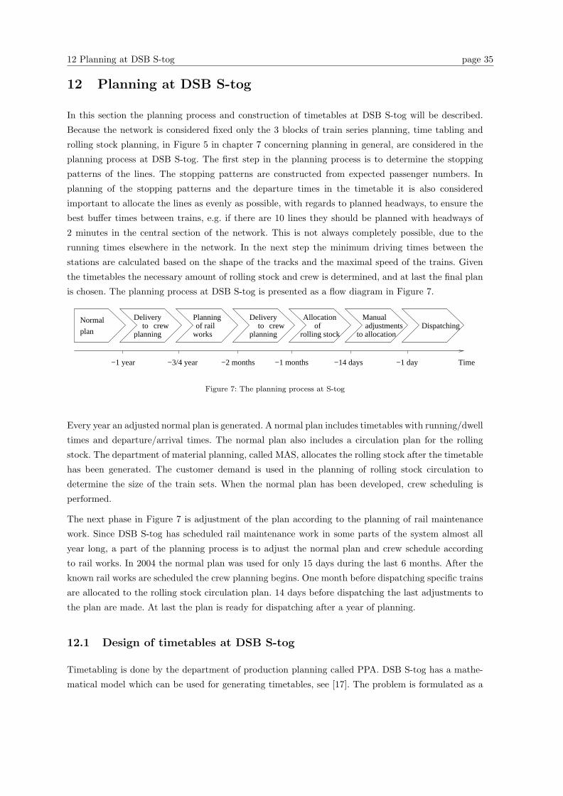
12 Planning at DSB S-tog page 35
12 Planning at DSB S-tog
In this section the planning process and construction of timetables at DSB S-tog will be described.
Because the network is considered fixed only the 3 blocks of train series planning, time tabling and
rolling stock planning, in Figure 5 in chapter 7 concerning planning in general, are considered in the
planning process at DSB S-tog. The first step in the planning process is to determine the stopping
patterns of the lines. The stopping patterns are constructed from expected passenger numbers. In
planning of the stopping patterns and the departure times in the timetable it is also considered
important to allocate the lines as evenly as possible, with regards to planned headways, to ensure the
best buffer times between trains, e.g. if there are 10 lines they should be planned with headways of
2 minutes in the central section of the network. This is not always completely possible, due to the
running times elsewhere in the network. In the next step the minimum driving times between the
stations are calculated based on the shape of the tracks and the maximal speed of the trains. Given
the timetables the necessary amount of rolling stock and crew is determined, and at last the final plan
is chosen. The planning process at DSB S-tog is presented as a flow diagram in Figure 7.
Time
Normal
plan
Planningof rail
works
Allocation of
rolling stock
Manualadjustments
to allocationDispatching
−1 year −3/4 year −2 months −1 months −14 days −1 day
Deliveryto crew
planning
Deliveryto crew
planning
Figure 7: The planning process at S-tog
Every year an adjusted normal plan is generated. A normal plan includes timetables with running/dwell
times and departure/arrival times. The normal plan also includes a circulation plan for the rolling
stock. The department of material planning, called MAS, allocates the rolling stock after the timetable
has been generated. The customer demand is used in the planning of rolling stock circulation to
determine the size of the train sets. When the normal plan has been developed, crew scheduling is
performed.
The next phase in Figure 7 is adjustment of the plan according to the planning of rail maintenance
work. Since DSB S-tog has scheduled rail maintenance work in some parts of the system almost all
year long, a part of the planning process is to adjust the normal plan and crew schedule according
to rail works. In 2004 the normal plan was used for only 15 days during the last 6 months. After the
known rail works are scheduled the crew planning begins. One month before dispatching specific trains
are allocated to the rolling stock circulation plan. 14 days before dispatching the last adjustments to
the plan are made. At last the plan is ready for dispatching after a year of planning.
12.1 Design of timetables at DSB S-tog
Timetabling is done by the department of production planning called PPA. DSB S-tog has a mathe-
matical model which can be used for generating timetables, see [17]. The problem is formulated as a

12.1 Design of timetables at DSB S-tog page 36
mixed integer problem (MIP). The MIP model is implemented in GAMS and solved by the MIP solver
in CPLEX. The cost of operating a given timetable is proportional to the number of trains required to
run the plan. Therefore the main objective in the MIP model is to minimize the number of train sets
necessary. An additional objective is to minimize the time between departures at certain stations e.g.
København, in cases where several lines cover the same series. The inputs to the model are the defined
train series network, the stopping pattern for each line, the running times between the stations, the
dwell time at stations, a requirement of 20 minute frequencies on all lines and scheduled headways of
2 minutes in the central section. The model does not take customer demand into account. The main
decision variables in the model are the departure times from each station for each line. The output
from the model is a timetable.
To make the timetable robust against disturbances, slack time is incorporated. Dwell times are adapted
to the expected number of passengers and disruption patterns at each station. Running times are
increased with a buffer of approximately 3.6 seconds pr. kilometre in certain places in the network.
Also at the end stations slack is added to minimize the risk of new trips being affected by the lateness
from the subsequent trips.

13 Circulation of rolling stock at DSB S-tog page 37
13 Circulation of rolling stock at DSB S-tog
In this chapter circulation of rolling stock at DSB S-tog will be described.
13.1 Rolling stock at DSB S-tog
DSB S-tog use 3 different types of trains called 2nd, 3rd and 4th generation, where the 4th generation
trains are the newest. In Table 1 the 2003 numbers of the 3 different train types are seen. In 2005
lines A and E between Køge or Hundige and Hillerød are covered by the new fourth generation trains,
because this series has been improved to be able to handle the speed of this train type. Lines B, C
and H can be covered by all three types of trains. Ringbanen, line F, is always covered by the third
generation trains. In 2006 all the S-train lines should be covered by 4th generation trains. It is not
possible to make any combination of the trains across the three different generations. The S-trains are
powered by electricity.
Type Number of trains Set type
2nd generation 5 2-coach
61 4-coach
3rd generation 8 4-coach train sets
4th generation 83 8-coach train sets
Table 1: S-trains rolling stock at the end of 2003
There are several different material depots, where trains can be stored or shunting can occur. These de-
pots are at København, Høje Taastrup, Køge, Hillerød, Hundige, Farum, Frederikssund, Klampenborg
and Ballerup.
Maintenance of the trains can only be done at Høje Taastrup station, so all the trains have to terminate
at this station within given intervals to get a service inspection. A train can normally drive 22.000
kilometres or approximately 60 days before a maintenance check is needed. The only prepare centre
is in Hundige, where external cleaning of the trains is carried out. Internal cleaning can be handled at
most of the large stations.
13.2 Circulation plan
After the timetable is constructed the allocation of rolling stock is scheduled. First it is planned how
many train units and which types are needed for each line but not exactly which specific train units.
The lengths of the trains are determined from the customer demand, but the maximum length of a
train is limited by the shortest platform in the network. The plan for the circulation of rolling stock
indicates how many train units of each type are needed on a specific line on a specific day.
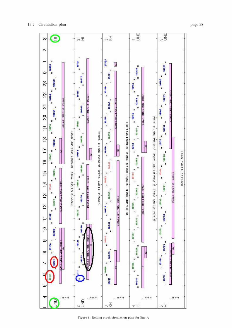
13.2 Circulation plan page 38
Figure 8: Rolling stock circulation plan for line A
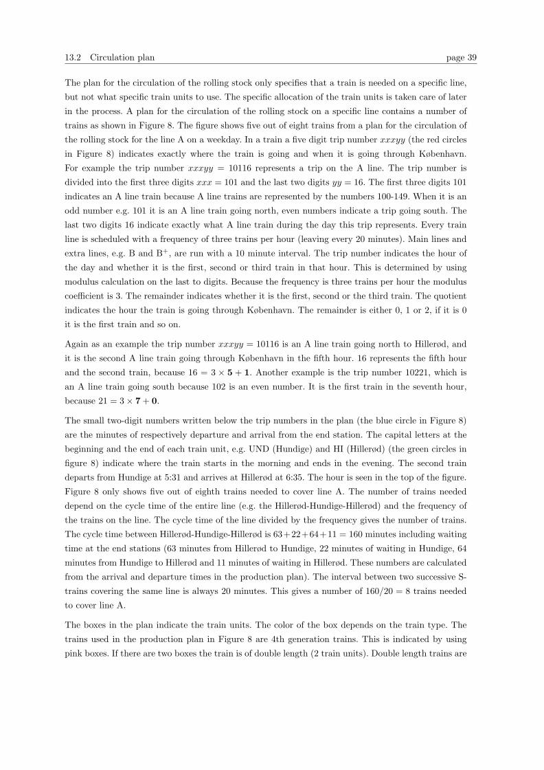
13.2 Circulation plan page 39
The plan for the circulation of the rolling stock only specifies that a train is needed on a specific line,
but not what specific train units to use. The specific allocation of the train units is taken care of later
in the process. A plan for the circulation of the rolling stock on a specific line contains a number of
trains as shown in Figure 8. The figure shows five out of eight trains from a plan for the circulation of
the rolling stock for the line A on a weekday. In a train a five digit trip number xxxyy (the red circles
in Figure 8) indicates exactly where the train is going and when it is going through København.
For example the trip number xxxyy = 10116 represents a trip on the A line. The trip number is
divided into the first three digits xxx = 101 and the last two digits yy = 16. The first three digits 101
indicates an A line train because A line trains are represented by the numbers 100-149. When it is an
odd number e.g. 101 it is an A line train going north, even numbers indicate a trip going south. The
last two digits 16 indicate exactly what A line train during the day this trip represents. Every train
line is scheduled with a frequency of three trains per hour (leaving every 20 minutes). Main lines and
extra lines, e.g. B and B+, are run with a 10 minute interval. The trip number indicates the hour of
the day and whether it is the first, second or third train in that hour. This is determined by using
modulus calculation on the last to digits. Because the frequency is three trains per hour the modulus
coefficient is 3. The remainder indicates whether it is the first, second or the third train. The quotient
indicates the hour the train is going through København. The remainder is either 0, 1 or 2, if it is 0
it is the first train and so on.
Again as an example the trip number xxxyy = 10116 is an A line train going north to Hillerød, and
it is the second A line train going through København in the fifth hour. 16 represents the fifth hour
and the second train, because 16 = 3 × 5 + 1. Another example is the trip number 10221, which is
an A line train going south because 102 is an even number. It is the first train in the seventh hour,
because 21 = 3× 7 + 0.
The small two-digit numbers written below the trip numbers in the plan (the blue circle in Figure 8)
are the minutes of respectively departure and arrival from the end station. The capital letters at the
beginning and the end of each train unit, e.g. UND (Hundige) and HI (Hillerød) (the green circles in
figure 8) indicate where the train starts in the morning and ends in the evening. The second train
departs from Hundige at 5:31 and arrives at Hillerød at 6:35. The hour is seen in the top of the figure.
Figure 8 only shows five out of eighth trains needed to cover line A. The number of trains needed
depend on the cycle time of the entire line (e.g. the Hillerød-Hundige-Hillerød) and the frequency of
the trains on the line. The cycle time of the line divided by the frequency gives the number of trains.
The cycle time between Hillerød-Hundige-Hillerød is 63+22+64+11 = 160 minutes including waiting
time at the end stations (63 minutes from Hillerød to Hundige, 22 minutes of waiting in Hundige, 64
minutes from Hundige to Hillerød and 11 minutes of waiting in Hillerød. These numbers are calculated
from the arrival and departure times in the production plan). The interval between two successive S-
trains covering the same line is always 20 minutes. This gives a number of 160/20 = 8 trains needed
to cover line A.
The boxes in the plan indicate the train units. The color of the box depends on the train type. The
trains used in the production plan in Figure 8 are 4th generation trains. This is indicated by using
pink boxes. If there are two boxes the train is of double length (2 train units). Double length trains are
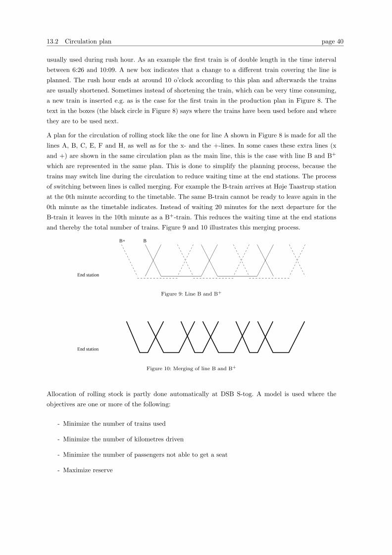
13.2 Circulation plan page 40
usually used during rush hour. As an example the first train is of double length in the time interval
between 6:26 and 10:09. A new box indicates that a change to a different train covering the line is
planned. The rush hour ends at around 10 o’clock according to this plan and afterwards the trains
are usually shortened. Sometimes instead of shortening the train, which can be very time consuming,
a new train is inserted e.g. as is the case for the first train in the production plan in Figure 8. The
text in the boxes (the black circle in Figure 8) says where the trains have been used before and where
they are to be used next.
A plan for the circulation of rolling stock like the one for line A shown in Figure 8 is made for all the
lines A, B, C, E, F and H, as well as for the x- and the +-lines. In some cases these extra lines (x
and +) are shown in the same circulation plan as the main line, this is the case with line B and B+
which are represented in the same plan. This is done to simplify the planning process, because the
trains may switch line during the circulation to reduce waiting time at the end stations. The process
of switching between lines is called merging. For example the B-train arrives at Høje Taastrup station
at the 0th minute according to the timetable. The same B-train cannot be ready to leave again in the
0th minute as the timetable indicates. Instead of waiting 20 minutes for the next departure for the
B-train it leaves in the 10th minute as a B+-train. This reduces the waiting time at the end stations
and thereby the total number of trains. Figure 9 and 10 illustrates this merging process.
End station
BB+
Figure 9: Line B and B+
End station
Figure 10: Merging of line B and B+
Allocation of rolling stock is partly done automatically at DSB S-tog. A model is used where the
objectives are one or more of the following:
- Minimize the number of trains used
- Minimize the number of kilometres driven
- Minimize the number of passengers not able to get a seat
- Maximize reserve

13.2 Circulation plan page 41
- Maximize seats.
This model is used to optimize the rolling stock used in the rush hour. The model is also used to
examine the requirement for rolling stock and in some of the phases of allocation of rolling stock
combined with manual scheduling work.
As mentioned in chapter 12 new circulation plans are created when the timetable is improved once
a year. The circulation planners make these plans in a specified program, where they build up the
plan by hand using drag and drop. It is made from experience and the changes in the timetable are
often small, which enables the planners to reuse some sequences of the old plans. The circulation
plans also include periodic maintenance of the trains. About 2 months before the new timetable is
published actual train sets are attached to the rolling stock plan. This is mostly done automatically.
As a main rule the same trains run the same lines day after day, this minimizes dead heading of
the trains (transport without passengers). During the next period after the circulation plan has been
completed, the situation is monitored to adjust the new timetable, if any changes occur because of
acute track maintenance or severe disturbances.
When the new timetable is published and running, the network is monitored from a control centre,
and different recovery strategies are used if and when disturbances occur. This phase is examined in
chapter 15.
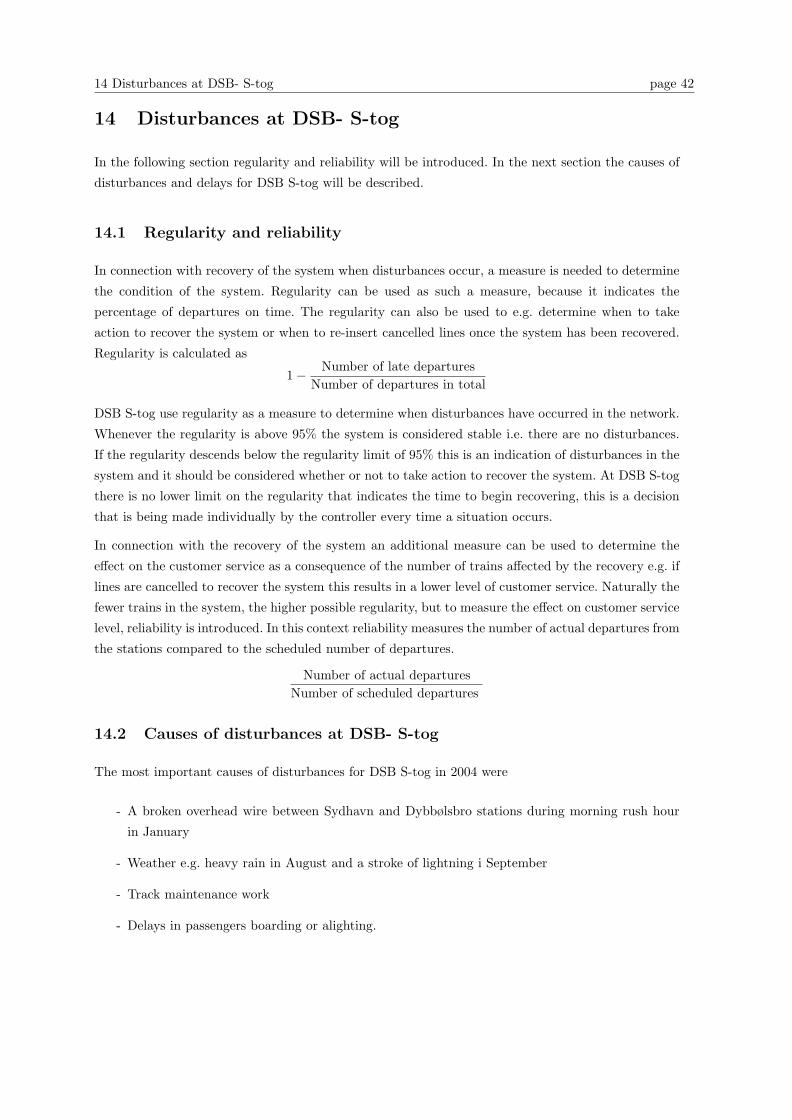
14 Disturbances at DSB- S-tog page 42
14 Disturbances at DSB- S-tog
In the following section regularity and reliability will be introduced. In the next section the causes of
disturbances and delays for DSB S-tog will be described.
14.1 Regularity and reliability
In connection with recovery of the system when disturbances occur, a measure is needed to determine
the condition of the system. Regularity can be used as such a measure, because it indicates the
percentage of departures on time. The regularity can also be used to e.g. determine when to take
action to recover the system or when to re-insert cancelled lines once the system has been recovered.
Regularity is calculated as
1− Number of late departuresNumber of departures in total
DSB S-tog use regularity as a measure to determine when disturbances have occurred in the network.
Whenever the regularity is above 95% the system is considered stable i.e. there are no disturbances.
If the regularity descends below the regularity limit of 95% this is an indication of disturbances in the
system and it should be considered whether or not to take action to recover the system. At DSB S-tog
there is no lower limit on the regularity that indicates the time to begin recovering, this is a decision
that is being made individually by the controller every time a situation occurs.
In connection with the recovery of the system an additional measure can be used to determine the
effect on the customer service as a consequence of the number of trains affected by the recovery e.g. if
lines are cancelled to recover the system this results in a lower level of customer service. Naturally the
fewer trains in the system, the higher possible regularity, but to measure the effect on customer service
level, reliability is introduced. In this context reliability measures the number of actual departures from
the stations compared to the scheduled number of departures.
Number of actual departuresNumber of scheduled departures
14.2 Causes of disturbances at DSB- S-tog
The most important causes of disturbances for DSB S-tog in 2004 were
- A broken overhead wire between Sydhavn and Dybbølsbro stations during morning rush hour
in January
- Weather e.g. heavy rain in August and a stroke of lightning i September
- Track maintenance work
- Delays in passengers boarding or alighting.
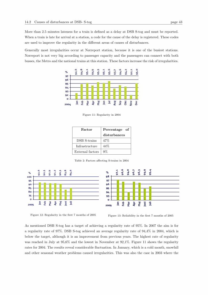
14.2 Causes of disturbances at DSB- S-tog page 43
More than 2.5 minutes lateness for a train is defined as a delay at DSB S-tog and must be reported.
When a train is late for arrival at a station, a code for the cause of the delay is registered. These codes
are used to improve the regularity in the different areas of causes of disturbances.
Generally most irregularities occur at Nørreport station, because it is one of the busiest stations.
Nørreport is not very big according to passenger capacity and the passengers can connect with both
busses, the Metro and the national trains at this station. These factors increase the risk of irregularities.
Figure 11: Regularity in 2004
Factor Percentage of
disturbances
DSB S-trains 47%
Infrastructure 44%
External factors 9%
Table 2: Factors affecting S-trains in 2004
Figure 12: Regularity in the first 7 months of 2005 Figure 13: Reliability in the first 7 months of 2005
As mentioned DSB S-tog has a target of achieving a regularity rate of 95%. In 2007 the aim is for
a regularity rate of 97%. DSB S-tog achieved an average regularity rate of 94,4% in 2004, which is
below the target, although it is an improvement from previous years. The highest rate of regularity
was reached in July at 95,6% and the lowest in November at 92,1%. Figure 11 shows the regularity
rates for 2004. The results reveal considerable fluctuation. In January, which is a cold month, snowfall
and other seasonal weather problems caused irregularities. This was also the case in 2003 where the
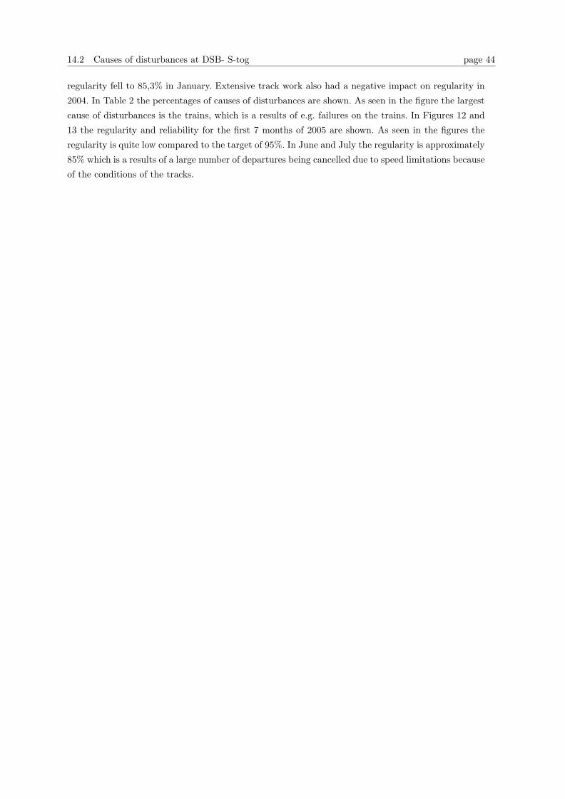
14.2 Causes of disturbances at DSB- S-tog page 44
regularity fell to 85,3% in January. Extensive track work also had a negative impact on regularity in
2004. In Table 2 the percentages of causes of disturbances are shown. As seen in the figure the largest
cause of disturbances is the trains, which is a results of e.g. failures on the trains. In Figures 12 and
13 the regularity and reliability for the first 7 months of 2005 are shown. As seen in the figures the
regularity is quite low compared to the target of 95%. In June and July the regularity is approximately
85% which is a results of a large number of departures being cancelled due to speed limitations because
of the conditions of the tracks.
15 Recovery strategies and methods at DSB S-tog page 45
15 Recovery strategies and methods at DSB S-tog
In this chapter recovery strategies and methods used at DSB S-tog will be described. Furthermore it
is explained how the recovery methods are implemented. Some of the practical requirements that need
to be taken care of during recovery will also be examined.
15.1 Recovery strategies
When the S-train network is influenced by disturbances different kinds of changes are applied to the
system to recover from the disruptions. When changes are made, the passengers are informed, to make
sure that the disturbances affect them as little as possible. In situations with delays the controller will
try to recover by re-establishing the original plan, in order to avoid affection the passengers more than
necessary. If the disturbances make it impossible to re-establish the original plan, re-scheduling will
have to take place.
15.1.1 Re-establishing strategies
When disturbances occur in the S-train network all planned marshalling to larger or smaller size is
cancelled. This is done to use the time more effective on recovering instead of creating further delays.
Also if delays have occurred, more passengers may be waiting at the station so if the train has to leave
the station within the scheduled dwell time it can be an advantage if the train has already marshalled
to larger size to leave it like this.
Platform changes on-the-day are being used e.g. if a train arrives late at the terminal station it might
be re-scheduled to the platform where it has the next departure.
A train may skip some of the smaller stations if delays occur e.g. a B line train on the way from
Hellerup to Holte may stop at Lyngby only and skip all stations in between (like the A and E line
trains). In this case passengers will be advices on an earlier station, to give them the possibility of
changing train.
A late train may turn around before the end station and continue in the opposite direction according
to the plan. For example an A line train going to Hillerød can turn around in Holte if it is sufficiently
late.
If a fast train catches up with a slower train due to delays and it is impossible for the fast train to
pass the slow train, the two trains may swap ’identity’ or running patterns on the next station, so
the first train leaves as a fast train and the latter train becomes a slow train. As an example if an H
line train catches up with a C line train on the way to Vanløse, the C line train which is in front may
continue from Vanløse as an H line train, and then the H line train will continue as a C line train.
If large delays influence a specific train e.g. an A line train, a new A line train can be inserted at
København to leave on the scheduled time. When the delayed A line train arrives at København it
is simply taken out. The passengers in the delayed train will have to leave the train at København
15.1 Recovery strategies page 46
and take the next train. Considering that the train was already late these passengers are of course
further delayed, but at the same time all other passengers planning to use the train from København
can continue their travel without delays.
When trains are put out of order, so that they will have to be repaired before they can be used again,
the controller tries to insert a replacement train to take over the trip whenever possible. Replacement
trains are usually scheduled to begin their trip from København, since this is where both trains and
crew are available in reserve.
Reducing dwell times to a minimum is possible at all the stations in the network. The train driver
can decide to reduce the dwell time in order to reduce to delay. Reducing headways to a minimum
is possible at some of the longer stretches of tracks, usually in the ends of the train series. Reducing
running times might be possible in few sections of the network, when disturbances occur. A system
exists that informs the train driver on which speed he should drive in order to keep the distance to
the preceding train.
The order of the trains follows a specific sequence given by the timetable. This sequence is only
broken if large delays occur. Changes in the order are not always easy. Overtaking can only take place
at stations with more than one track in the same direction or at places in the network with double
tracks. Only few stations have double tracks, which makes overtaking rare. If a train is delayed at
arrival to a station all other trains scheduled for arrival later at the same platform are held back
until the delayed train has arrived, unless the controller informs the system to react otherwise. The
controllers learn by experience how much a train must be delayed before they have to take action and
change the order of trains.
15.1.2 Re-scheduling strategies
When the sizes of the disturbances make it impossible to re-establish the original plan, the controller
needs to re-schedule the trains.
One of the strategies that DSB S-tog use is that when large disturbances occur, the +-lines and x-lines
are cancelled. This results in larger headways which may reduce delays considerably. As of today DSB
S-tog never plan re-insertion of cancelled lines the same day. All recovery is done with regards to
execution of normal schedule the following morning.
If disturbances block the traffic somewhere in the central section between Svanemøllen and København
e.g. at Nørreport, then the train lines are divided into a northern part and a southern part that circulate
between the end stations and the blocked station.
All recovery strategies are evaluated according to estimates on the capacity of free rolling stock and
available personnel. Sometimes when irregularities occur there are too few train drivers to re-establish
the normal schedule. This is a limitation for recovery.
15.2 Recovery implementation methods and practical requirements page 47
15.2 Recovery implementation methods and practical requirements
At DSB S-tog the different recovery strategies and methods are not implemented in an automatic
decision system. A decision about using a specific recovery method in a given situation is typically
based on experience. A rule book concerning which methods to use exists but is rarely used. Plans
for the future is to update this rule book and make some of the decision automatic and concerning
both materiel and personnel. This new system should be able to generate solutions automatically, for
restoring the normal operations plan. It should also be possible to evaluate several feasible solutions
with regards to quality e.g. robustness and total recovery time in real-time.
DSB S-tog has a system that shows the original plan as it was in the morning. This can be of great
help to determine where the trains are located in the system at a given time. This information is very
important to the controller, when he or she needs to make a new plan or re-schedule the trains. The
system can be used for manually re-scheduling the trains.
A system for generating solutions for re-inserting cancelled trains is under development. When lines
are cancelled, the trains are taken out at the depots. When re-inserting the trains, crew needs to be
transported to the depots. Given a train which is the first possible for transporting crew to the depots,
the system can generate a solution that takes care of the order of re-insertion of the trains. The system
only generates feasible solutions and does not take into consideration the quality of the solutions.
Trains running on lines that are cancelled for the rest of the day, are shunted to the shunting yards at
the end stations where they are scheduled for the following morning. Defective train units are shunted
to the maintenance yard in time according to the gravity of the faults, meaning that if the train is
severely damaged it is taken directly to the maintenance yard, whereas if it is only a minor fault, e.g.
a door that cannot open, it may continue the trip for the rest of the day.
If disturbances and delays have occurred in the system during the day, the main goal for recovering is
to ensure the necessary number of train units are at each depot at the end of the day to prepare for the
scheduled traffic the following morning. Sometimes less important maintenance schedules are cancelled
to keep the necessary number of trains on the tracks the next day. The different defects on the trains
are reported and categorized in the production plan, so the controller can use this information to
cancel or postpone less crucial maintenance in the planning of recovery.
16 Arena and description of the first models page 48
16 Arena and description of the first models
In this chapter an introduction and description of the simulation program Arena will be given. Only
the elements of Arena used in the models in this project will be explained. We have learned about
Arena by reading the text book [12]. To illustrate our learning process with Arena, the use of Arena
will be examined through two of the models, made before the final model of the S-train network was
build. Starting with a very simple model in section 16.2, where the subject of routing between two
stations was explored. In Model 2 in section 16.3 three entire stations were build with concern of dwell
time, delay, headways, fast routes etc. First Arena is described in general.
16.1 Arena
At the highest level of abstraction, Arena deals with entities, resources, variables, attributes and
events. Entities are the elements that traverse the model during simulation e.g. the trains. Resources
can represent processes and other static assets in the model e.g. stations and tracks. Variables are all
the adjustable or changing parts of the model e.g. running times and dwell times. Variables are global
and pertain the whole model as opposed to attributes, which are entity specific variables representing
characteristics for the different entities in the model. An attribute only pertain the entity it is connected
to. An example of an attribute can be the time the entity should be disposed and leave the system.
This can be specific for each entity and can be stored in an attribute. If the value is used in other
correlations, not only including the specific entity, the value should be stored in a variable. Finally
events are all the things that happen during the run of the simulation. Variables and attributes might
be changed during an event. Examples of events are arrivals and departures, or when an entity enters
or leaves the model.
When building a simulation model in Arena the basic building blocks are modules. The modules are
split into two categories: flowchart modules and data modules, see Figure 14 and 15.
Figure 14: Flowchart Module Figure 15: Data Module
Flowchart modules describe the dynamic processes, the movements and the changes in the model.
The data for the flowchart modules can be specified in the associated dialog boxes. These modules
are connected to indicate the movement of the entities in the model. The data modules define the
characteristics of different elements like entities, queues and resources. They are also used to set
variables or expressions that pertain the whole model.
At a lower level of abstraction, elements and blocks can be used instead of modules. Basic process
modules often have some of the same features as elements and blocks, but not with the same level of
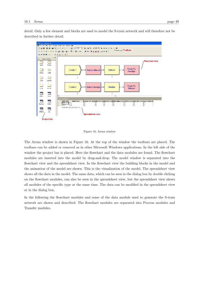
16.1 Arena page 49
detail. Only a few element and blocks are used to model the S-train network and will therefore not be
described in further detail.
Figure 16: Arena window
The Arena window is shown in Figure 16. At the top of the window the toolbars are placed. The
toolbars can be added or removed as in other Microsoft Windows applications. In the left side of the
window the project bar is placed. Here the flowchart and the data modules are found. The flowchart
modules are inserted into the model by drag-and-drop. The model window is separated into the
flowchart view and the spreadsheet view. In the flowchart view the building blocks in the model and
the animation of the model are shown. This is the visualization of the model. The spreadsheet view
shows all the data in the model. The same data, which can be seen in the dialog box by double clicking
on the flowchart modules, can also be seen in the spreadsheet view, but the spreadsheet view shows
all modules of the specific type at the same time. The data can be modified in the spreadsheet view
or in the dialog box.
In the following the flowchart modules and some of the data module used to generate the S-train
network are shown and described. The flowchart modules are separated into Process modules and
Transfer modules.
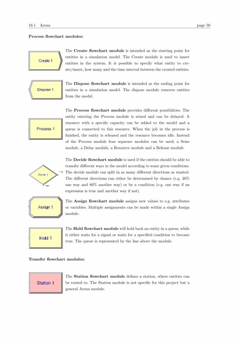
16.1 Arena page 50
Process flowchart modules:
The Create flowchart module is intended as the starting point for
entities in a simulation model. The Create module is used to insert
entities in the system. It is possible to specify what entity to cre-
ate/insert, how many and the time interval between the created entities.
The Dispose flowchart module is intended as the ending point for
entities in a simulation model. The dispose module removes entities
from the model.
The Process flowchart module provides different possibilities. The
entity entering the Process module is seized and can be delayed. A
resource with a specific capacity can be added to the model and a
queue is connected to this resource. When the job in the process is
finished, the entity is released and the resource becomes idle. Instead
of the Process module four separate modules can be used; a Seize
module, a Delay module, a Resource module and a Release module.
The Decide flowchart module is used if the entities should be able to
transfer different ways in the model according to some given conditions.
The decide module can split in as many different directions as wanted.
The different directions can either be determined by chance (e.g. 20%
one way and 80% another way) or by a condition (e.g. one way if an
expression is true and another way if not).
The Assign flowchart module assigns new values to e.g. attributes
or variables. Multiple assignments can be made within a single Assign
module.
The Hold flowchart module will hold back an entity in a queue, while
it either waits for a signal or waits for a specified condition to become
true. The queue is represented by the line above the module.
Transfer flowchart modules:
The Station flowchart module defines a station, where entities can
be routed to. The Station module is not specific for this project but a
general Arena module.

16.1 Arena page 51
The Route flowchart module transfers an entity to a specified sta-
tion, or the next station in the station visitation sequence defined for
the entity. A delay time to transfer to the next station can be defined.
If a Route module is not used, the travel time between two flowchart
modules is zero.
Data modules:
The Entity data module defines the various entity types and their
initial picture values in a simulation. Entities can be defined in the
Entity data module or a new entity will automatically be defined when
used for the first time in a flowchart module. The entity pictures can be
edited (see the menu Edit-Entity Picture). Various colored trains are
made to match particular S-train lines in the models in this project.
The Queue data module may be utilized to change the ranking
rule for a specified queue. The default ranking rule for all queues is
first-in-first-out.
The Variable data module is used to define the dimension and
initial value(s) of the variables. A variable can represent a single value,
an array or a matrix of values. Variables can be referred to in other
modules (e.g. the Decide module), can be reassigned a new value with
the Assign module or can be used in any expression.
The Advanced Set data module specifies queue sets, entity sets and
other sets and their respective members. A set defines a group of simi-
lar elements that may be referenced via a common name and a set index.
Examples of how these different modules are used are seen in the following sections. All the modules
except the Route and Station modules are connected using the Connect button on the toolbar, see
Figure 17. Then the entities will travel from module to module during the simulation. The travel time
on the connections are zero, as mentioned Route modules are used when the travel time between two
modules should not be zero.
Figure 17: Connect button
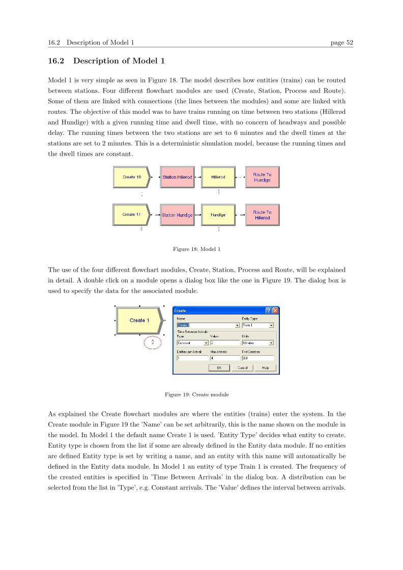
16.2 Description of Model 1 page 52
16.2 Description of Model 1
Model 1 is very simple as seen in Figure 18. The model describes how entities (trains) can be routed
between stations. Four different flowchart modules are used (Create, Station, Process and Route).
Some of them are linked with connections (the lines between the modules) and some are linked with
routes. The objective of this model was to have trains running on time between two stations (Hillerød
and Hundige) with a given running time and dwell time, with no concern of headways and possible
delay. The running times between the two stations are set to 6 minutes and the dwell times at the
stations are set to 2 minutes. This is a deterministic simulation model, because the running times and
the dwell times are constant.
Figure 18: Model 1
The use of the four different flowchart modules, Create, Station, Process and Route, will be explained
in detail. A double click on a module opens a dialog box like the one in Figure 19. The dialog box is
used to specify the data for the associated module.
Figure 19: Create module
As explained the Create flowchart modules are where the entities (trains) enter the system. In the
Create module in Figure 19 the ’Name’ can be set arbitrarily, this is the name shown on the module in
the model. In Model 1 the default name Create 1 is used. ’Entity Type’ decides what entity to create.
Entity type is chosen from the list if some are already defined in the Entity data module. If no entities
are defined Entity type is set by writing a name, and an entity with this name will automatically be
defined in the Entity data module. In Model 1 an entity of type Train 1 is created. The frequency of
the created entities is specified in ’Time Between Arrivals’ in the dialog box. A distribution can be
selected from the list in ’Type’, e.g. Constant arrivals. The ’Value’ defines the interval between arrivals.
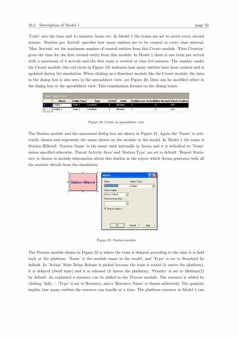
16.2 Description of Model 1 page 53
’Units’ sets the time unit to minutes, hours etc. In Model 1 the trains are set to arrive every second
minute. ’Entities per Arrival’ specifies how many entities are to be created at every time interval.
’Max Arrivals’ set the maximum number of created entities from this Create module. ’First Creation’
gives the time for the first created entity from this module. In Model 1 there is one train per arrival
with a maximum of 4 arrivals and the first train is created at time 0.0 minutes. The number under
the Create module (the red circle in Figure 19) indicates how many entities have been created and is
updated during the simulation. When clicking on a flowchart module like the Create module, the data
in the dialog box is also seen in the spreadsheet view, see Figure 20. Data can be modified either in
the dialog box or the spreadsheet view. This examination focuses on the dialog boxes.
Figure 20: Create in spreadsheet view
The Station module and the associated dialog box are shown in Figure 21. Again the ’Name’ is arbi-
trarily chosen and represents the name shown on the module in the model. In Model 1 the name is
Station Hillerød. ’Station Name’ is the name used internally in Arena and it is defaulted to ’Name’
unless specified otherwise. ’Parent Activity Area’ and ’Station Type’ are set to default. ’Report Statis-
tics’ is chosen to include information about this station in the report which Arena generates with all
the statistic details from the simulation.
Figure 21: Station module
The Process module shown in Figure 22 is where the train is delayed according to the time it is held
back at the platform. ’Name’ is the module name in the model, and ’Type’ is set to Standard by
default. In ’Action’ Seize Delay Release is picked because the train is seized (it enters the platform),
it is delayed (dwell time) and it is released (it leaves the platform). ’Priority’ is set to Medium(2)
by default. As explained a resource can be added to the Process module. The resource is added by
clicking ’Add...’. ’Type’ is set to Resource, and a ’Resource Name’ is chosen arbitrarily. The quantity
implies how many entities the resource can handle at a time. The platform resource in Model 1 can
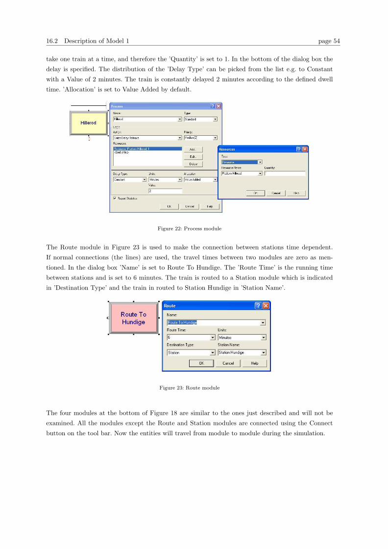
16.2 Description of Model 1 page 54
take one train at a time, and therefore the ’Quantity’ is set to 1. In the bottom of the dialog box the
delay is specified. The distribution of the ’Delay Type’ can be picked from the list e.g. to Constant
with a Value of 2 minutes. The train is constantly delayed 2 minutes according to the defined dwell
time. ’Allocation’ is set to Value Added by default.
Figure 22: Process module
The Route module in Figure 23 is used to make the connection between stations time dependent.
If normal connections (the lines) are used, the travel times between two modules are zero as men-
tioned. In the dialog box ’Name’ is set to Route To Hundige. The ’Route Time’ is the running time
between stations and is set to 6 minutes. The train is routed to a Station module which is indicated
in ’Destination Type’ and the train in routed to Station Hundige in ’Station Name’.
Figure 23: Route module
The four modules at the bottom of Figure 18 are similar to the ones just described and will not be
examined. All the modules except the Route and Station modules are connected using the Connect
button on the tool bar. Now the entities will travel from module to module during the simulation.
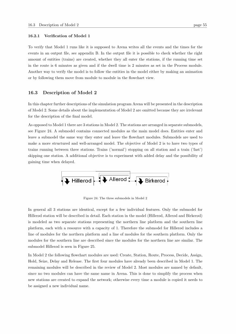
16.3 Description of Model 2 page 55
16.2.1 Verification of Model 1
To verify that Model 1 runs like it is supposed to Arena writes all the events and the times for the
events in an output file, see appendix B. In the output file it is possible to check whether the right
amount of entities (trains) are created, whether they all enter the stations, if the running time set
in the route is 6 minutes as given and if the dwell time is 2 minutes as set in the Process module.
Another way to verify the model is to follow the entities in the model either by making an animation
or by following them move from module to module in the flowchart view.
16.3 Description of Model 2
In this chapter further descriptions of the simulation program Arena will be presented in the description
of Model 2. Some details about the implementation of Model 2 are omitted because they are irrelevant
for the description of the final model.
As opposed to Model 1 there are 3 stations in Model 2. The stations are arranged in separate submodels,
see Figure 24. A submodel contains connected modules as the main model does. Entities enter and
leave a submodel the same way they enter and leave the flowchart modules. Submodels are used to
make a more structured and well-arranged model. The objective of Model 2 is to have two types of
trains running between three stations. Trains (’normal’) stopping on all station and a train (’fast’)
skipping one station. A additional objective is to experiment with added delay and the possibility of
gaining time when delayed.
Figure 24: The three submodels in Model 2
In general all 3 stations are identical, except for a few individual features. Only the submodel for
Hillerød station will be described in detail. Each station in the model (Hillerød, Allerød and Birkerød)
is modeled as two separate stations representing the northern line platform and the southern line
platform, each with a resource with a capacity of 1. Therefore the submodel for Hillerød includes a
line of modules for the northern platform and a line of modules for the southern platform. Only the
modules for the southern line are described since the modules for the northern line are similar. The
submodel Hillerød is seen in Figure 25.
In Model 2 the following flowchart modules are used: Create, Station, Route, Process, Decide, Assign,
Hold, Seize, Delay and Release. The first four modules have already been described in Model 1. The
remaining modules will be described in the review of Model 2. Most modules are named by default,
since no two modules can have the same name in Arena. This is done to simplify the process when
new stations are created to expand the network; otherwise every time a module is copied it needs to
be assigned a new individual name.
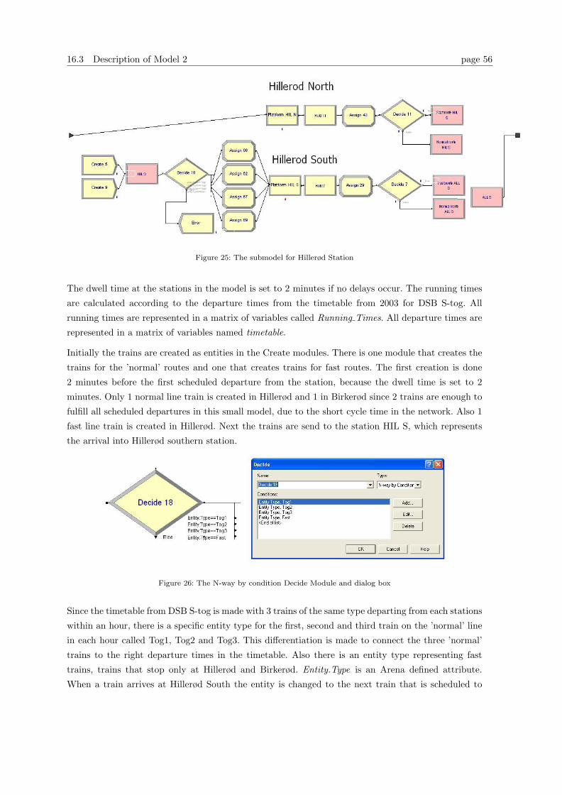
16.3 Description of Model 2 page 56
Figure 25: The submodel for Hillerød Station
The dwell time at the stations in the model is set to 2 minutes if no delays occur. The running times
are calculated according to the departure times from the timetable from 2003 for DSB S-tog. All
running times are represented in a matrix of variables called Running Times. All departure times are
represented in a matrix of variables named timetable.
Initially the trains are created as entities in the Create modules. There is one module that creates the
trains for the ’normal’ routes and one that creates trains for fast routes. The first creation is done
2 minutes before the first scheduled departure from the station, because the dwell time is set to 2
minutes. Only 1 normal line train is created in Hillerød and 1 in Birkerød since 2 trains are enough to
fulfill all scheduled departures in this small model, due to the short cycle time in the network. Also 1
fast line train is created in Hillerød. Next the trains are send to the station HIL S, which represents
the arrival into Hillerød southern station.
Figure 26: The N-way by condition Decide Module and dialog box
Since the timetable from DSB S-tog is made with 3 trains of the same type departing from each stations
within an hour, there is a specific entity type for the first, second and third train on the ’normal’ line
in each hour called Tog1, Tog2 and Tog3. This differentiation is made to connect the three ’normal’
trains to the right departure times in the timetable. Also there is an entity type representing fast
trains, trains that stop only at Hillerød and Birkerød. Entity.Type is an Arena defined attribute.
When a train arrives at Hillerød South the entity is changed to the next train that is scheduled to
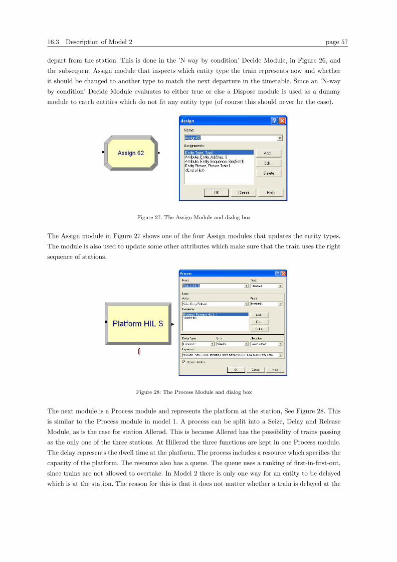
16.3 Description of Model 2 page 57
depart from the station. This is done in the ’N-way by condition’ Decide Module, in Figure 26, and
the subsequent Assign module that inspects which entity type the train represents now and whether
it should be changed to another type to match the next departure in the timetable. Since an ’N-way
by condition’ Decide Module evaluates to either true or else a Dispose module is used as a dummy
module to catch entities which do not fit any entity type (of course this should never be the case).
Figure 27: The Assign Module and dialog box
The Assign module in Figure 27 shows one of the four Assign modules that updates the entity types.
The module is also used to update some other attributes which make sure that the train uses the right
sequence of stations.
Figure 28: The Process Module and dialog box
The next module is a Process module and represents the platform at the station, See Figure 28. This
is similar to the Process module in model 1. A process can be split into a Seize, Delay and Release
Module, as is the case for station Allerød. This is because Allerød has the possibility of trains passing
as the only one of the three stations. At Hillerød the three functions are kept in one Process module.
The delay represents the dwell time at the platform. The process includes a resource which specifies the
capacity of the platform. The resource also has a queue. The queue uses a ranking of first-in-first-out,
since trains are not allowed to overtake. In Model 2 there is only one way for an entity to be delayed
which is at the station. The reason for this is that it does not matter whether a train is delayed at the
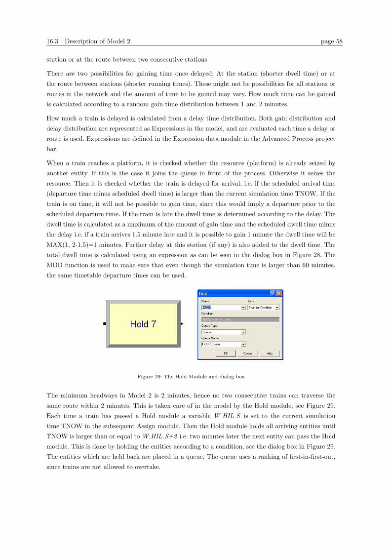
16.3 Description of Model 2 page 58
station or at the route between two consecutive stations.
There are two possibilities for gaining time once delayed: At the station (shorter dwell time) or at
the route between stations (shorter running times). These might not be possibilities for all stations or
routes in the network and the amount of time to be gained may vary. How much time can be gained
is calculated according to a random gain time distribution between 1 and 2 minutes.
How much a train is delayed is calculated from a delay time distribution. Both gain distribution and
delay distribution are represented as Expressions in the model, and are evaluated each time a delay or
route is used. Expressions are defined in the Expression data module in the Advanced Process project
bar.
When a train reaches a platform, it is checked whether the resource (platform) is already seized by
another entity. If this is the case it joins the queue in front of the process. Otherwise it seizes the
resource. Then it is checked whether the train is delayed for arrival, i.e. if the scheduled arrival time
(departure time minus scheduled dwell time) is larger than the current simulation time TNOW. If the
train is on time, it will not be possible to gain time, since this would imply a departure prior to the
scheduled departure time. If the train is late the dwell time is determined according to the delay. The
dwell time is calculated as a maximum of the amount of gain time and the scheduled dwell time minus
the delay i.e. if a train arrives 1.5 minute late and it is possible to gain 1 minute the dwell time will be
MAX(1, 2-1.5)=1 minutes. Further delay at this station (if any) is also added to the dwell time. The
total dwell time is calculated using an expression as can be seen in the dialog box in Figure 28. The
MOD function is used to make sure that even though the simulation time is larger than 60 minutes,
the same timetable departure times can be used.
Figure 29: The Hold Module and dialog box
The minimum headways in Model 2 is 2 minutes, hence no two consecutive trains can traverse the
same route within 2 minutes. This is taken care of in the model by the Hold module, see Figure 29.
Each time a train has passed a Hold module a variable W HIL S is set to the current simulation
time TNOW in the subsequent Assign module. Then the Hold module holds all arriving entities until
TNOW is larger than or equal to W HIL S+2 i.e. two minutes later the next entity can pass the Hold
module. This is done by holding the entities according to a condition, see the dialog box in Figure 29.
The entities which are held back are placed in a queue. The queue uses a ranking of first-in-first-out,
since trains are not allowed to overtake.
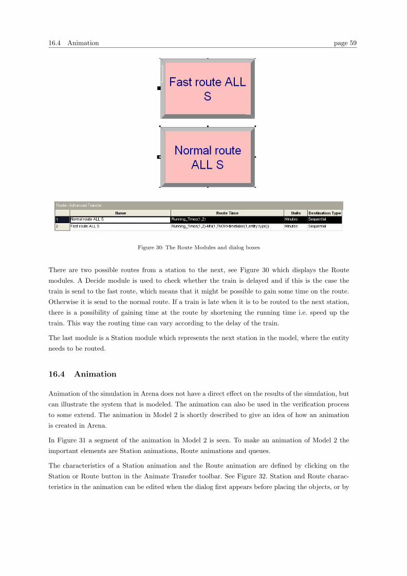
16.4 Animation page 59
Figure 30: The Route Modules and dialog boxes
There are two possible routes from a station to the next, see Figure 30 which displays the Route
modules. A Decide module is used to check whether the train is delayed and if this is the case the
train is send to the fast route, which means that it might be possible to gain some time on the route.
Otherwise it is send to the normal route. If a train is late when it is to be routed to the next station,
there is a possibility of gaining time at the route by shortening the running time i.e. speed up the
train. This way the routing time can vary according to the delay of the train.
The last module is a Station module which represents the next station in the model, where the entity
needs to be routed.
16.4 Animation
Animation of the simulation in Arena does not have a direct effect on the results of the simulation, but
can illustrate the system that is modeled. The animation can also be used in the verification process
to some extend. The animation in Model 2 is shortly described to give an idea of how an animation
is created in Arena.
In Figure 31 a segment of the animation in Model 2 is seen. To make an animation of Model 2 the
important elements are Station animations, Route animations and queues.
The characteristics of a Station animation and the Route animation are defined by clicking on the
Station or Route button in the Animate Transfer toolbar. See Figure 32. Station and Route charac-
teristics in the animation can be edited when the dialog first appears before placing the objects, or by
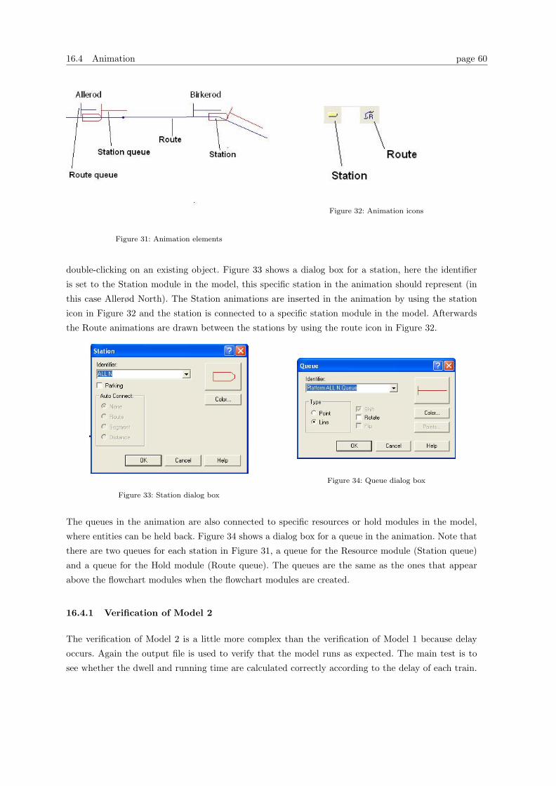
16.4 Animation page 60
Figure 31: Animation elements
Figure 32: Animation icons
double-clicking on an existing object. Figure 33 shows a dialog box for a station, here the identifier
is set to the Station module in the model, this specific station in the animation should represent (in
this case Allerød North). The Station animations are inserted in the animation by using the station
icon in Figure 32 and the station is connected to a specific station module in the model. Afterwards
the Route animations are drawn between the stations by using the route icon in Figure 32.
Figure 33: Station dialog box
Figure 34: Queue dialog box
The queues in the animation are also connected to specific resources or hold modules in the model,
where entities can be held back. Figure 34 shows a dialog box for a queue in the animation. Note that
there are two queues for each station in Figure 31, a queue for the Resource module (Station queue)
and a queue for the Hold module (Route queue). The queues are the same as the ones that appear
above the flowchart modules when the flowchart modules are created.
16.4.1 Verification of Model 2
The verification of Model 2 is a little more complex than the verification of Model 1 because delay
occurs. Again the output file is used to verify that the model runs as expected. The main test is to
see whether the dwell and running time are calculated correctly according to the delay of each train.
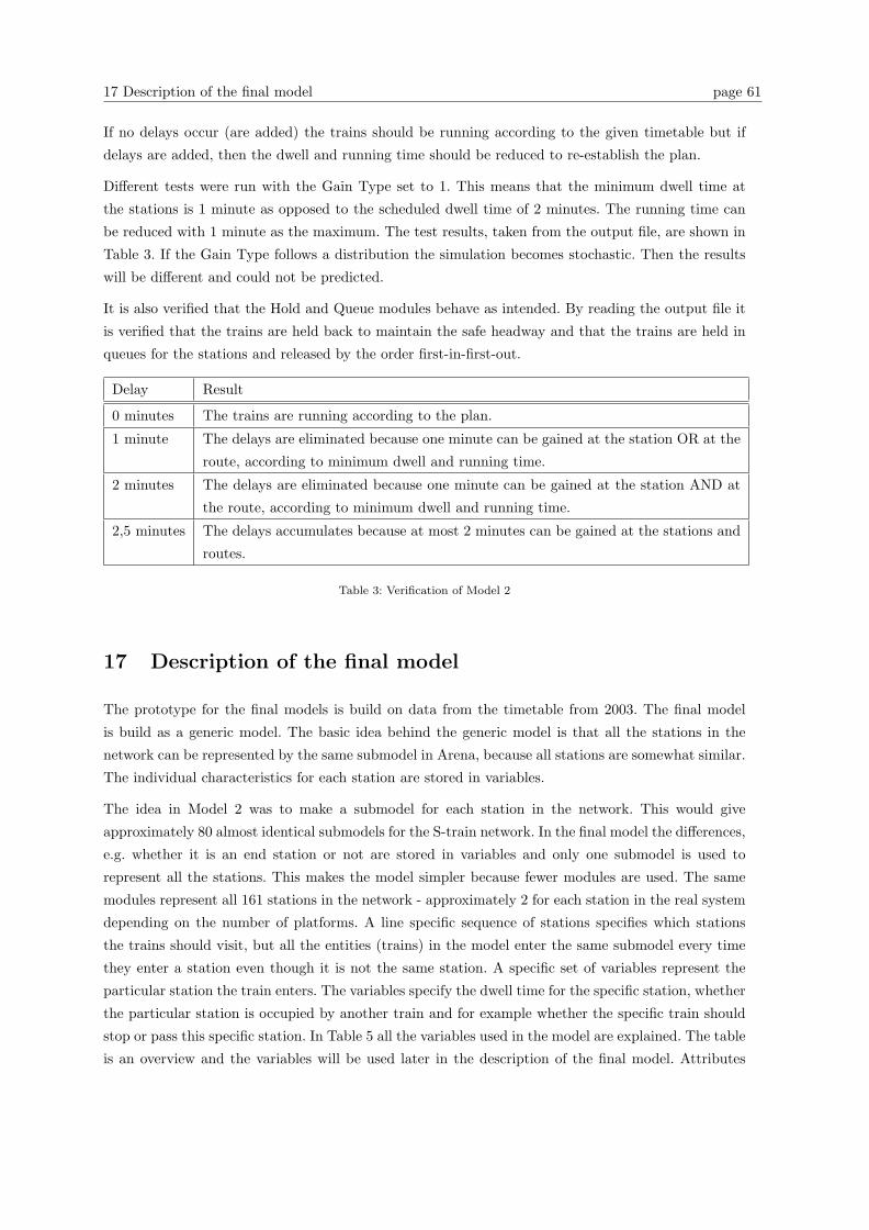
17 Description of the final model page 61
If no delays occur (are added) the trains should be running according to the given timetable but if
delays are added, then the dwell and running time should be reduced to re-establish the plan.
Different tests were run with the Gain Type set to 1. This means that the minimum dwell time at
the stations is 1 minute as opposed to the scheduled dwell time of 2 minutes. The running time can
be reduced with 1 minute as the maximum. The test results, taken from the output file, are shown in
Table 3. If the Gain Type follows a distribution the simulation becomes stochastic. Then the results
will be different and could not be predicted.
It is also verified that the Hold and Queue modules behave as intended. By reading the output file it
is verified that the trains are held back to maintain the safe headway and that the trains are held in
queues for the stations and released by the order first-in-first-out.
Delay Result
0 minutes The trains are running according to the plan.
1 minute The delays are eliminated because one minute can be gained at the station OR at the
route, according to minimum dwell and running time.
2 minutes The delays are eliminated because one minute can be gained at the station AND at
the route, according to minimum dwell and running time.
2,5 minutes The delays accumulates because at most 2 minutes can be gained at the stations and
routes.
Table 3: Verification of Model 2
17 Description of the final model
The prototype for the final models is build on data from the timetable from 2003. The final model
is build as a generic model. The basic idea behind the generic model is that all the stations in the
network can be represented by the same submodel in Arena, because all stations are somewhat similar.
The individual characteristics for each station are stored in variables.
The idea in Model 2 was to make a submodel for each station in the network. This would give
approximately 80 almost identical submodels for the S-train network. In the final model the differences,
e.g. whether it is an end station or not are stored in variables and only one submodel is used to
represent all the stations. This makes the model simpler because fewer modules are used. The same
modules represent all 161 stations in the network - approximately 2 for each station in the real system
depending on the number of platforms. A line specific sequence of stations specifies which stations
the trains should visit, but all the entities (trains) in the model enter the same submodel every time
they enter a station even though it is not the same station. A specific set of variables represent the
particular station the train enters. The variables specify the dwell time for the specific station, whether
the particular station is occupied by another train and for example whether the specific train should
stop or pass this specific station. In Table 5 all the variables used in the model are explained. The table
is an overview and the variables will be used later in the description of the final model. Attributes
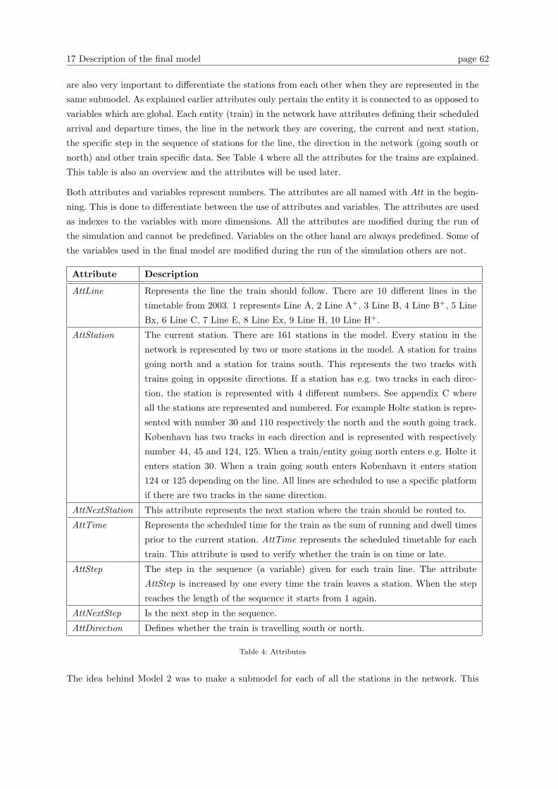
17 Description of the final model page 62
are also very important to differentiate the stations from each other when they are represented in the
same submodel. As explained earlier attributes only pertain the entity it is connected to as opposed to
variables which are global. Each entity (train) in the network have attributes defining their scheduled
arrival and departure times, the line in the network they are covering, the current and next station,
the specific step in the sequence of stations for the line, the direction in the network (going south or
north) and other train specific data. See Table 4 where all the attributes for the trains are explained.
This table is also an overview and the attributes will be used later.
Both attributes and variables represent numbers. The attributes are all named with Att in the begin-
ning. This is done to differentiate between the use of attributes and variables. The attributes are used
as indexes to the variables with more dimensions. All the attributes are modified during the run of
the simulation and cannot be predefined. Variables on the other hand are always predefined. Some of
the variables used in the final model are modified during the run of the simulation others are not.
Attribute Description
AttLine Represents the line the train should follow. There are 10 different lines in the
timetable from 2003. 1 represents Line A, 2 Line A+, 3 Line B, 4 Line B+, 5 Line
Bx, 6 Line C, 7 Line E, 8 Line Ex, 9 Line H, 10 Line H+.
AttStation The current station. There are 161 stations in the model. Every station in the
network is represented by two or more stations in the model. A station for trains
going north and a station for trains south. This represents the two tracks with
trains going in opposite directions. If a station has e.g. two tracks in each direc-
tion, the station is represented with 4 different numbers. See appendix C where
all the stations are represented and numbered. For example Holte station is repre-
sented with number 30 and 110 respectively the north and the south going track.
København has two tracks in each direction and is represented with respectively
number 44, 45 and 124, 125. When a train/entity going north enters e.g. Holte it
enters station 30. When a train going south enters København it enters station
124 or 125 depending on the line. All lines are scheduled to use a specific platform
if there are two tracks in the same direction.
AttNextStation This attribute represents the next station where the train should be routed to.
AttTime Represents the scheduled time for the train as the sum of running and dwell times
prior to the current station. AttTime represents the scheduled timetable for each
train. This attribute is used to verify whether the train is on time or late.
AttStep The step in the sequence (a variable) given for each train line. The attribute
AttStep is increased by one every time the train leaves a station. When the step
reaches the length of the sequence it starts from 1 again.
AttNextStep Is the next step in the sequence.
AttDirection Defines whether the train is travelling south or north.
Table 4: Attributes
The idea behind Model 2 was to make a submodel for each of all the stations in the network. This

17 Description of the final model page 63
Array of variables Description
Dwell(AttStation) The variable Dwell is an array with 161 rows with dwell times for the 161
stations in the model. See appendix D
MinDwell(AttStation) The variable MinDwell is also an array with 161 rows with minimum dwell
times for the 161 stations.
Running(AttStep,AttLine) Is an array defining running times between stations for all lines. The longest
line defines the first dimension of the array and the number of lines defines the
second dimension. See appendix E
Occup(AttStation) This array with 161 variables is used to make sure that there is only 1 train at
the station at a time. The variable is set to one for a particular station, when
a train enters this station. It is set to zero when the train leaves the station.
This way only one train can visit each station at the time even though all the
stations are represented by the same submodel.
Headways(AttStation) This array with 161 variables defines the headways after the particular station.
Headways are the minimum time interval between two consecutive trains.
WaitHeadways(AttStation) When a train leaves a station WaitHeadways(AttStation) is set to the current
simulation time (TNOW). The next train leaving the same station is held until
TNOW is greater than WaitHeadways(AttStation) + Headways(AttStation) to
make sure the right headways are kept on the routes between stations even
though all the routes are represented by the same submodel.
StationTypes(AttStation,AttLine) Indicates whether the train on the given line should stop on the specific sta-
tion. If StationTypes(AttStation,AttLine)= 1 the train should stop, if Station-
Types(AttStation,AttLine)= 3 the train should not stop on this station and
if StationTypes(AttStation,AttLine)= 2 the station is an end station. Virum
station is e.g. represented with a 1 for lines B/B+ and a 3 for lines A and E.
Holte station is represented with a 2 for lines B/B+ because these two lines
terminate in Holte and a 1 for lines A and E. See appendix F
Sequence(AttStep,AttLine) The sequence of all the stations on each line, including the stations where the
trains covering the line does not stop. For example the sequence for line A is
(Hillerød, Allerød, Birkerød, Holte, Virum, . . ., Ishøj, Hundige, . . ., Hillerød).
The sequence represents the stations in both directions. The sequence, as all
other variables, are represented with numbers. See appendix G
SequenceLength(AttLine) The lengths of the sequences for all lines.
MinShunt(AttStation,AttLine) The minimum shunting time at the end stations defined as the minimum time
required to turn around at the specific end station.
ChooseRec This variable is set to 0, 1, 2 or 3 defining whether no recovery method is used
(set to 0) or whether one of the 3 recovery methods are used (set to 1, 2 or 3).
A Branch module in the station submodel leads to one of the four choices.
WarmUp Because all trains are inserted at the end stations for each line, there is a warm
up period before the system is actually running according to the situation in
the real world. Regularity is not calculated during the warm up period and
delay are not added until TNOW is greater than the warm up time. The warm
up period is set to 250 minutes, because this is approximately how long time
it takes before all the trains are running.
MaxNoNextQueue This variable is used to hold back trains if the queue for the next station is to
long.
Table 5: Variables and Arrays in Main Model

17.1 Main model page 64
approach would have been time consuming but easy to implement, because the small differences at
the stations could be implemented directly in the submodel representing the specific station, but very
challenging to maintain because even few changes would have to be repeated for all station submodels.
Furthermore it would have been a lot of work to copy-paste and connect all the station submodels.
The final model needs a few more variables to separate the stations from each other when all stations
are represented by the same modules, but this also means that changes only have to made once and
the model becomes more well-arranged.
The final model can be split into separate parts:
- The main model, where entities (trains) are created.
- Station submodel, representing all the stations in the network.
- Two submodels where regularity and reliability are calculated.
- Three submodels with the three recovery methods.
- A submodel that reads running and dwell times from Excel and writes regularity data to text
files.
- Animation.
These different parts of the model will all be described in the following sections.
17.1 Main model
The main model is where the different entities (trains) are created and entering the system. The main
model is shown in Figure 35. 10 different types of entities are created for the model of the timetable
from 2003, one for each line in the network. The number of created entities of each type depends on
the number of train units needed to cover the line with an interval of 20 minutes between each train.
Table 6 shows the different entity types, the quantity created and the station they enter first. Each
entity is created according to the first departure time in the timetable and then every 20 minutes the
next entities are created.
Every Create module in the main model is followed by an Assign module, where the important at-
tributes AttLine, AttTime, AttStep and AttStation for each train are assigned. The attribute AttLine
depends on the line the created train should cover, AttTime is set to TNOW (the current simulation
time), the time the entity is created and AttStep is set to 1. All entities are created in the north end
because the first station in the sequences are the north end station. The attribute AttStation is set
to the first station, given by Sequence(AttStep,AttLine). The only assignment that are different for
the 10 different Assign modules are AttLine, which depends on the type of the train.
The next Assign module ’Choose Recovery Method 0 or 1 to 3’ assigns the variable ChooseRec to
0,1,2 or 3. If ChooseRec = 0 no recovery method is activated. Otherwise one of the three recovery
methods are used later in the model.
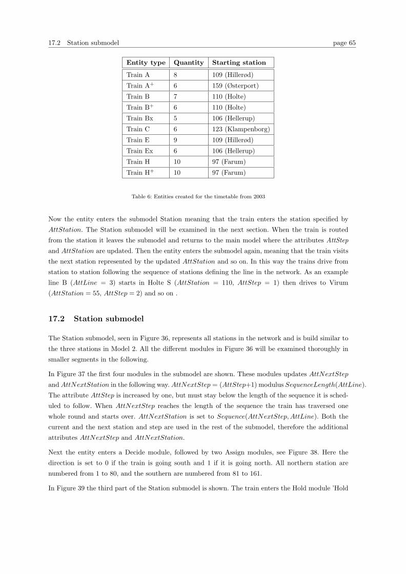
17.2 Station submodel page 65
Entity type Quantity Starting station
Train A 8 109 (Hillerød)
Train A+ 6 159 (Østerport)
Train B 7 110 (Holte)
Train B+ 6 110 (Holte)
Train Bx 5 106 (Hellerup)
Train C 6 123 (Klampenborg)
Train E 9 109 (Hillerød)
Train Ex 6 106 (Hellerup)
Train H 10 97 (Farum)
Train H+ 10 97 (Farum)
Table 6: Entities created for the timetable from 2003
Now the entity enters the submodel Station meaning that the train enters the station specified by
AttStation. The Station submodel will be examined in the next section. When the train is routed
from the station it leaves the submodel and returns to the main model where the attributes AttStep
and AttStation are updated. Then the entity enters the submodel again, meaning that the train visits
the next station represented by the updated AttStation and so on. In this way the trains drive from
station to station following the sequence of stations defining the line in the network. As an example
line B (AttLine = 3) starts in Holte S (AttStation = 110, AttStep = 1) then drives to Virum
(AttStation = 55, AttStep = 2) and so on .
17.2 Station submodel
The Station submodel, seen in Figure 36, represents all stations in the network and is build similar to
the three stations in Model 2. All the different modules in Figure 36 will be examined thoroughly in
smaller segments in the following.
In Figure 37 the first four modules in the submodel are shown. These modules updates AttNextStep
and AttNextStation in the following way. AttNextStep = (AttStep+1) modulus SequenceLength(AttLine).
The attribute AttStep is increased by one, but must stay below the length of the sequence it is sched-
uled to follow. When AttNextStep reaches the length of the sequence the train has traversed one
whole round and starts over. AttNextStation is set to Sequence(AttNextStep, AttLine). Both the
current and the next station and step are used in the rest of the submodel, therefore the additional
attributes AttNextStep and AttNextStation.
Next the entity enters a Decide module, followed by two Assign modules, see Figure 38. Here the
direction is set to 0 if the train is going south and 1 if it is going north. All northern station are
numbered from 1 to 80, and the southern are numbered from 81 to 161.
In Figure 39 the third part of the Station submodel is shown. The train enters the Hold module ’Hold
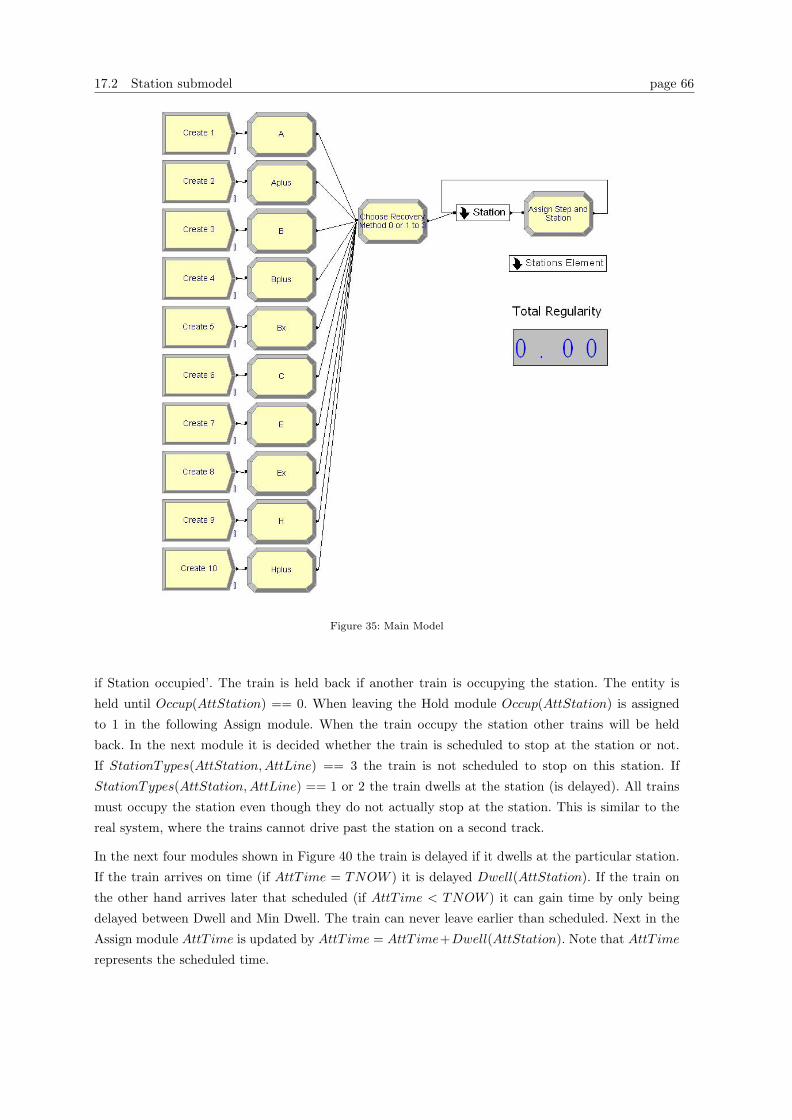
17.2 Station submodel page 66
Figure 35: Main Model
if Station occupied’. The train is held back if another train is occupying the station. The entity is
held until Occup(AttStation) == 0. When leaving the Hold module Occup(AttStation) is assigned
to 1 in the following Assign module. When the train occupy the station other trains will be held
back. In the next module it is decided whether the train is scheduled to stop at the station or not.
If StationTypes(AttStation, AttLine) == 3 the train is not scheduled to stop on this station. If
StationTypes(AttStation, AttLine) == 1 or 2 the train dwells at the station (is delayed). All trains
must occupy the station even though they do not actually stop at the station. This is similar to the
real system, where the trains cannot drive past the station on a second track.
In the next four modules shown in Figure 40 the train is delayed if it dwells at the particular station.
If the train arrives on time (if AttT ime = TNOW ) it is delayed Dwell(AttStation). If the train on
the other hand arrives later that scheduled (if AttT ime < TNOW ) it can gain time by only being
delayed between Dwell and Min Dwell. The train can never leave earlier than scheduled. Next in the
Assign module AttT ime is updated by AttT ime = AttT ime+Dwell(AttStation). Note that AttT ime
represents the scheduled time.
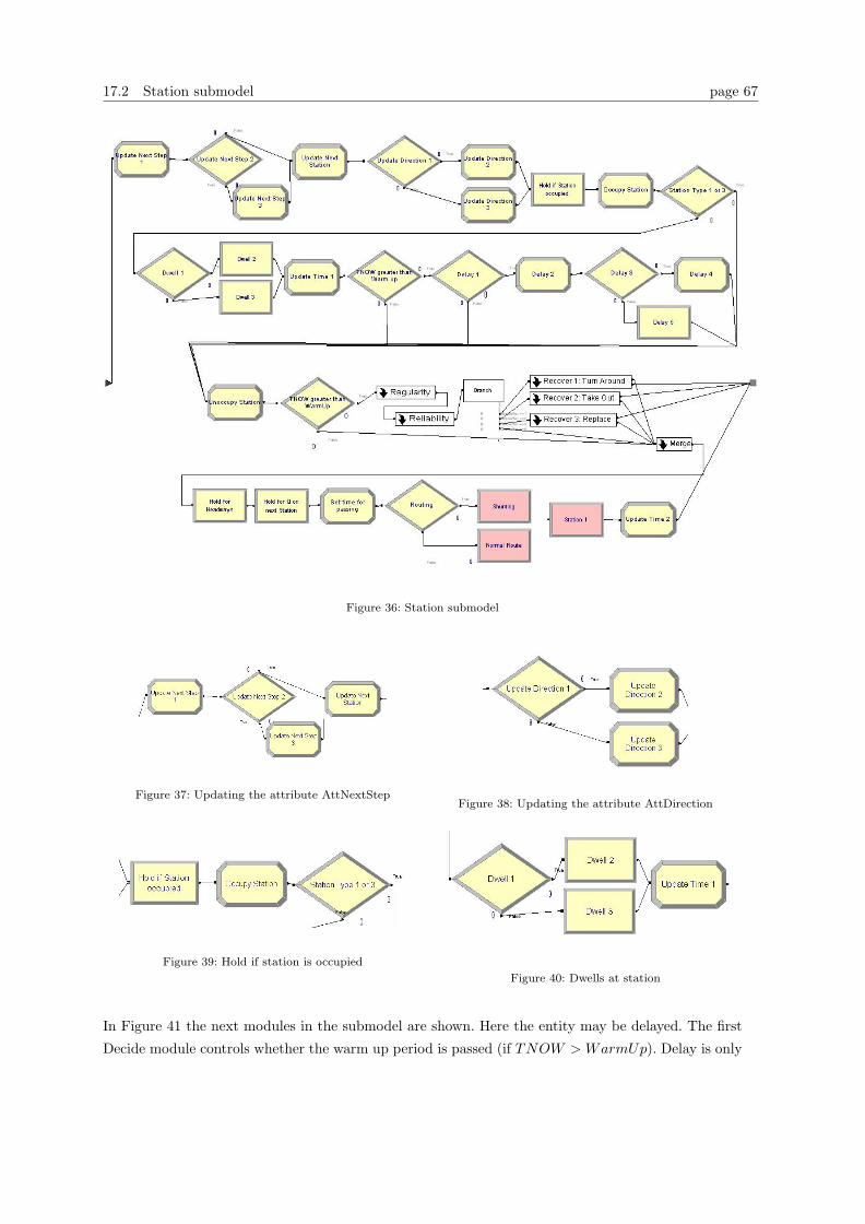
17.2 Station submodel page 67
Figure 36: Station submodel
Figure 37: Updating the attribute AttNextStepFigure 38: Updating the attribute AttDirection
Figure 39: Hold if station is occupied
Figure 40: Dwells at station
In Figure 41 the next modules in the submodel are shown. Here the entity may be delayed. The first
Decide module controls whether the warm up period is passed (if TNOW > WarmUp). Delay is only
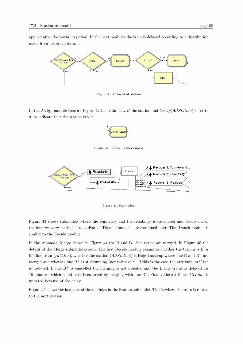
17.2 Station submodel page 68
applied after the warm up period. In the next modules the train is delayed according to a distribution
made from historical data.
Figure 41: Delayed at station
In the Assign module shown i Figure 42 the train ’leaves’ the station and Occup(AttStation) is set to
0, to indicate that the station is idle.
Figure 42: Station is unoccupied
Figure 43: Submodels
Figure 43 shows submodels where the regularity and the reliability is calculated and where one of
the four recovery methods are activated. These submodels are examined later. The Branch module is
similar to the Decide module.
In the submodel Merge shown in Figure 44 the B and B+ line trains are merged. In Figure 45 the
details of the Merge submodel is seen. The first Decide module examines whether the train is a B or
B+ line train (AttLine), whether the station (AttStation) is Høje Taastrup where line B and B+ are
merged and whether line B+ is still running (not taken out). If this is the case the attribute AttLine
is updated. If line B+ is cancelled the merging is not possible and the B line trains is delayed for
10 minutes, which could have been saved by merging with line B+. Finally the attribute AttT ime is
updated because of the delay.
Figure 46 shows the last part of the modules in the Station submodel. This is where the train is routed
to the next station.
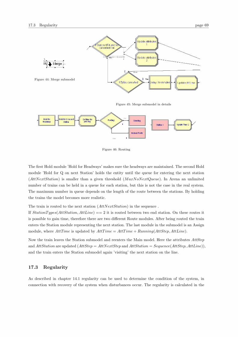
17.3 Regularity page 69
Figure 44: Merge submodel
Figure 45: Merge submodel in details
Figure 46: Routing
The first Hold module ’Hold for Headways’ makes sure the headways are maintained. The second Hold
module ’Hold for Q on next Station’ holds the entity until the queue for entering the next station
(AttNextStation) is smaller than a given threshold (MaxNoNextQueue). In Arena an unlimited
number of trains can be held in a queue for each station, but this is not the case in the real system.
The maximum number in queue depends on the length of the route between the stations. By holding
the trains the model becomes more realistic.
The train is routed to the next station (AttNextStation) in the sequence .
If StationTypes(AttStation, AttLine) == 2 it is routed between two end station. On these routes it
is possible to gain time, therefore there are two different Route modules. After being routed the train
enters the Station module representing the next station. The last module in the submodel is an Assign
module, where AttTime is updated by AttT ime = AttT ime + Running(AttStep,AttLine).
Now the train leaves the Station submodel and reenters the Main model. Here the attributes AttStep
and AttStation are updated (AttStep = AttNextStep and AttStation = Sequence(AttStep,AttLine)),
and the train enters the Station submodel again ’visiting’ the next station on the line.
17.3 Regularity
As described in chapter 14.1 regularity can be used to determine the condition of the system, in
connection with recovery of the system when disturbances occur. The regularity is calculated in the
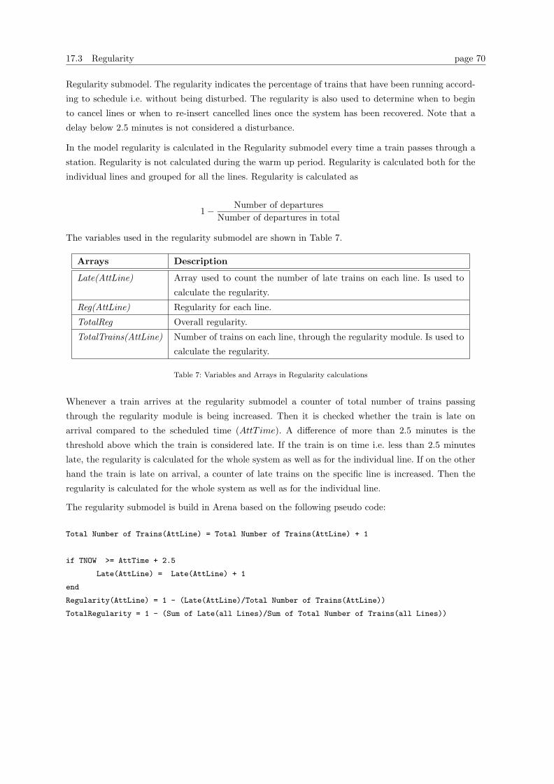
17.3 Regularity page 70
Regularity submodel. The regularity indicates the percentage of trains that have been running accord-
ing to schedule i.e. without being disturbed. The regularity is also used to determine when to begin
to cancel lines or when to re-insert cancelled lines once the system has been recovered. Note that a
delay below 2.5 minutes is not considered a disturbance.
In the model regularity is calculated in the Regularity submodel every time a train passes through a
station. Regularity is not calculated during the warm up period. Regularity is calculated both for the
individual lines and grouped for all the lines. Regularity is calculated as
1− Number of departuresNumber of departures in total
The variables used in the regularity submodel are shown in Table 7.
Arrays Description
Late(AttLine) Array used to count the number of late trains on each line. Is used to
calculate the regularity.
Reg(AttLine) Regularity for each line.
TotalReg Overall regularity.
TotalTrains(AttLine) Number of trains on each line, through the regularity module. Is used to
calculate the regularity.
Table 7: Variables and Arrays in Regularity calculations
Whenever a train arrives at the regularity submodel a counter of total number of trains passing
through the regularity module is being increased. Then it is checked whether the train is late on
arrival compared to the scheduled time (AttT ime). A difference of more than 2.5 minutes is the
threshold above which the train is considered late. If the train is on time i.e. less than 2.5 minutes
late, the regularity is calculated for the whole system as well as for the individual line. If on the other
hand the train is late on arrival, a counter of late trains on the specific line is increased. Then the
regularity is calculated for the whole system as well as for the individual line.
The regularity submodel is build in Arena based on the following pseudo code:
Total Number of Trains(AttLine) = Total Number of Trains(AttLine) + 1
if TNOW >= AttTime + 2.5
Late(AttLine) = Late(AttLine) + 1
end
Regularity(AttLine) = 1 - (Late(AttLine)/Total Number of Trains(AttLine))
TotalRegularity = 1 - (Sum of Late(all Lines)/Sum of Total Number of Trains(all Lines))
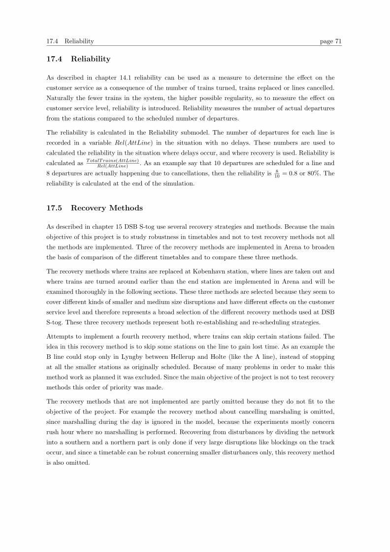
17.4 Reliability page 71
17.4 Reliability
As described in chapter 14.1 reliability can be used as a measure to determine the effect on the
customer service as a consequence of the number of trains turned, trains replaced or lines cancelled.
Naturally the fewer trains in the system, the higher possible regularity, so to measure the effect on
customer service level, reliability is introduced. Reliability measures the number of actual departures
from the stations compared to the scheduled number of departures.
The reliability is calculated in the Reliability submodel. The number of departures for each line is
recorded in a variable Rel(AttLine) in the situation with no delays. These numbers are used to
calculated the reliability in the situation where delays occur, and where recovery is used. Reliability is
calculated as TotalTrains(AttLine)Rel(AttLine) . As an example say that 10 departures are scheduled for a line and
8 departures are actually happening due to cancellations, then the reliability is 810 = 0.8 or 80%. The
reliability is calculated at the end of the simulation.
17.5 Recovery Methods
As described in chapter 15 DSB S-tog use several recovery strategies and methods. Because the main
objective of this project is to study robustness in timetables and not to test recovery methods not all
the methods are implemented. Three of the recovery methods are implemented in Arena to broaden
the basis of comparison of the different timetables and to compare these three methods.
The recovery methods where trains are replaced at København station, where lines are taken out and
where trains are turned around earlier than the end station are implemented in Arena and will be
examined thoroughly in the following sections. These three methods are selected because they seem to
cover different kinds of smaller and medium size disruptions and have different effects on the customer
service level and therefore represents a broad selection of the different recovery methods used at DSB
S-tog. These three recovery methods represent both re-establishing and re-scheduling strategies.
Attempts to implement a fourth recovery method, where trains can skip certain stations failed. The
idea in this recovery method is to skip some stations on the line to gain lost time. As an example the
B line could stop only in Lyngby between Hellerup and Holte (like the A line), instead of stopping
at all the smaller stations as originally scheduled. Because of many problems in order to make this
method work as planned it was excluded. Since the main objective of the project is not to test recovery
methods this order of priority was made.
The recovery methods that are not implemented are partly omitted because they do not fit to the
objective of the project. For example the recovery method about cancelling marshaling is omitted,
since marshalling during the day is ignored in the model, because the experiments mostly concern
rush hour where no marshalling is performed. Recovering from disturbances by dividing the network
into a southern and a northern part is only done if very large disruptions like blockings on the track
occur, and since a timetable can be robust concerning smaller disturbances only, this recovery method
is also omitted.
17.5 Recovery Methods page 72
17.5.1 Turn around before the end station
The idea in this recovery methods is that if a train is delayed more than it is possible to gain while
shunting at the end station or more than a maximum time e.g. 5 minutes, it will turn around at a
station prior to the end station.
At DSB S-tog this is a recovery method that is being used, and in principle it is possible to turn
around at all stations. In practice trains are only allowed to turn around at larger stations, to give
passengers a possibility of changing to other trains.
The stations in the model where it is possible to turn around are
- Ballerup - going south (except line C)
- Buddinge - going north
- Friheden - going south
- Glostrup - going south
- Hellerup - going north or south (except north for lines Bx and Ex)
- Holte - going north (except for lines B and B+)
- Hundige - going south (except line A)
- København - going north or south
- Lyngby - going north
- Vanløse - going south.
It is not possible to turn around in both directions, because a train should not be allowed to visit only
few stations and then turn around and run back. This assumption is made from a passenger service
perspective.
When a train on a specific line has just turned around, the following train on the same line is not
allowed to turn around. Otherwise it would be difficult for the customers to reach the outer stations
in the network when disturbances and delays occur. Hence when a train has been turned, the next
train is set to drive through to the end station, and then the next train again is allowed to turn etc.
In the model this is handled by setting a variable LineOut(AttLine) for the line to 1 when a train
has been turned, and then when the next train on the line (in the same direction) has reached the last
station on the line where it is possible to turn around the variable is set to 0 again, making it possible
for trains on the specific line to turn around. This should ensure that at least every second train runs
all the way to the end station.
When a train has been turned around at a station it is being inserted at the scheduled time AttTime,
where it should have left the station (going in the other direction). In the model the insertion is
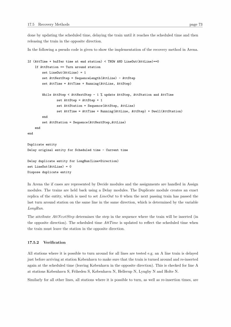
17.5 Recovery Methods page 73
done by updating the scheduled time, delaying the train until it reaches the scheduled time and then
releasing the train in the opposite direction.
In the following a pseudo code is given to show the implementation of the recovery method in Arena.
If (AttTime + buffer time at end station) < TNOW AND LineOut(AttLine)==0
If AttStation == Turn around station
set LineOut(AttLine) = 1
set AttNextStep = SequenceLength(AttLine) - AttStep
set AttTime = AttTime + Running(AttLine, AttStep)
While AttStep < AttNextStep - 1 % update AttStep, AttStation and AttTime
set AttStep = AttStep + 1
set AttStation = Sequence(AttStep, AttLine)
set AttTime = AttTime + Running(AttLine, AttStep) + Dwell(AttStation)
end
set AttStation = Sequence(AttNextStep,AttLine)
end
end
Duplicate entity
Delay original entity for Scheduled time - Current time
Delay duplicate entity for LongRun(Line+Direction)
set LineOut(AttLine) = 0
Dispose duplicate entity
In Arena the if cases are represented by Decide modules and the assignments are handled in Assign
modules. The trains are held back using a Delay modules. The Duplicate module creates an exact
replica of the entity, which is used to set LineOut to 0 when the next passing train has passed the
last turn around station on the same line in the same direction, which is determined by the variable
LongRun.
The attribute AttNextStep determines the step in the sequence where the train will be inserted (in
the opposite direction). The scheduled time AttTime is updated to reflect the scheduled time when
the train must leave the station in the opposite direction.
17.5.2 Verification
All stations where it is possible to turn around for all lines are tested e.g. an A line train is delayed
just before arriving at station København to make sure that the train is turned around and re-inserted
again at the scheduled time (leaving København in the opposite direction). This is checked for line A
at stations København S, Friheden S, København N, Hellerup N, Lyngby N and Holte N.
Similarly for all other lines, all stations where it is possible to turn, as well as re-insertion times, are
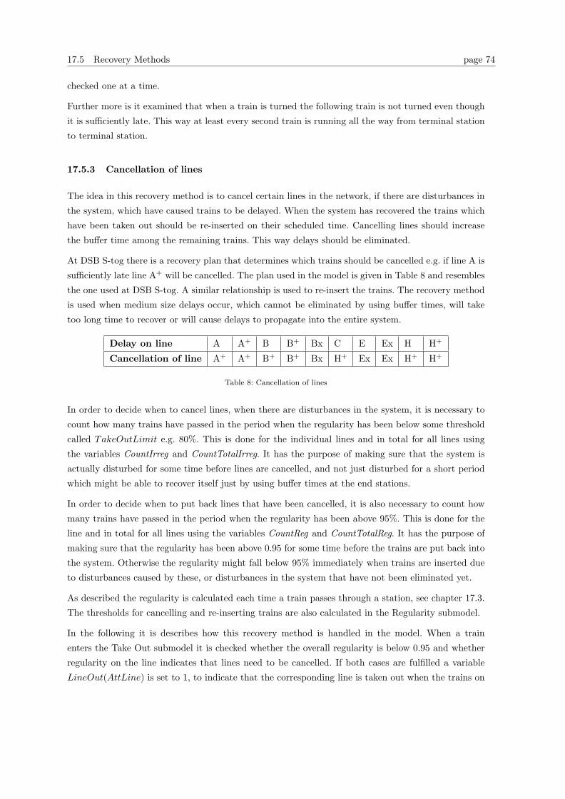
17.5 Recovery Methods page 74
checked one at a time.
Further more is it examined that when a train is turned the following train is not turned even though
it is sufficiently late. This way at least every second train is running all the way from terminal station
to terminal station.
17.5.3 Cancellation of lines
The idea in this recovery method is to cancel certain lines in the network, if there are disturbances in
the system, which have caused trains to be delayed. When the system has recovered the trains which
have been taken out should be re-inserted on their scheduled time. Cancelling lines should increase
the buffer time among the remaining trains. This way delays should be eliminated.
At DSB S-tog there is a recovery plan that determines which trains should be cancelled e.g. if line A is
sufficiently late line A+ will be cancelled. The plan used in the model is given in Table 8 and resembles
the one used at DSB S-tog. A similar relationship is used to re-insert the trains. The recovery method
is used when medium size delays occur, which cannot be eliminated by using buffer times, will take
too long time to recover or will cause delays to propagate into the entire system.
Delay on line A A+ B B+ Bx C E Ex H H+
Cancellation of line A+ A+ B+ B+ Bx H+ Ex Ex H+ H+
Table 8: Cancellation of lines
In order to decide when to cancel lines, when there are disturbances in the system, it is necessary to
count how many trains have passed in the period when the regularity has been below some threshold
called TakeOutLimit e.g. 80%. This is done for the individual lines and in total for all lines using
the variables CountIrreg and CountTotalIrreg. It has the purpose of making sure that the system is
actually disturbed for some time before lines are cancelled, and not just disturbed for a short period
which might be able to recover itself just by using buffer times at the end stations.
In order to decide when to put back lines that have been cancelled, it is also necessary to count how
many trains have passed in the period when the regularity has been above 95%. This is done for the
line and in total for all lines using the variables CountReg and CountTotalReg. It has the purpose of
making sure that the regularity has been above 0.95 for some time before the trains are put back into
the system. Otherwise the regularity might fall below 95% immediately when trains are inserted due
to disturbances caused by these, or disturbances in the system that have not been eliminated yet.
As described the regularity is calculated each time a train passes through a station, see chapter 17.3.
The thresholds for cancelling and re-inserting trains are also calculated in the Regularity submodel.
In the following it is describes how this recovery method is handled in the model. When a train
enters the Take Out submodel it is checked whether the overall regularity is below 0.95 and whether
regularity on the line indicates that lines need to be cancelled. If both cases are fulfilled a variable
LineOut(AttLine) is set to 1, to indicate that the corresponding line is taken out when the trains on

17.5 Recovery Methods page 75
the line reach a depot station. At the depot the trains are held back until the regularity has stabilized
above 0.95 again.
It is assumed in the model that trains can be taken out at depot stations only, which is also the case
in the real system. Depot stations are København, Hillerød, Farum, Frederikssund, Høje Taastrup,
Køge, Ballerup, Klampenborg and Hundige.
When trains are taken out at the depots there is not always enough personnel at the depots to be able
to put them back into the system, because the only personnel depot is at København. In the model it
is assumed that personnel will be available at all times to make it possible to re-insert trains.
In the following a pseudo code is given to show the case for an A line train which is late and the
corresponding A+ line which will be cancelled. The method is similar for all other lines. The method
consists of 3 parts: Adjust variables, Cancel line and Re-insert line.
if TotalRegularity <= 0.95
if CountIrreg(Line A) >= CountLimit
set LineOut(Line A+)=1 % Adjust variables
end
end
if AttStation == Depot AttStation AND LineOut(A+)==1 AND AttLine = 2 % (Line A+)
Hold train until LineOut(Line A+)==0 % Cancel line
When LineOut(Line A+)==0 %Re-insert line
Delay train until AttTime - AMOD(TNOW,TotalTourTime(Line A+))- Dwell(AttStation)
set AttTime = TNOW
set AttStep = AttStep - 1
set AttNextStep = AttNextStep - 1
set AttStation = Sequence(AttStep, AttLine)
set AttNextStation = Sequence(AttNextStep, AttLine)
end
end
if CountTotalReg >= PutBackLimit
set LineOut(Line A+)=0
end
AMOD is the real number remainder function in Arena. The amount of delay before re-insertion
depend on the cycle time stored in the variable TotalTourT ime. It is calculated in the following way
to make sure that the trains are re-inserted at the time when they would have left the station on
schedule.
As an example a train has a scheduled time for leaving København which is AttT ime = 107.5. The
line has been cancelled earlier and now the system has recovered to a regularity above 0.95, therefore
the line should be re-inserted. The TotalTourT ime for this line is 120 min. and the current time is
300. So the train should leave København at 107.5+2× 120 = 347.5 The current time 300 is given by
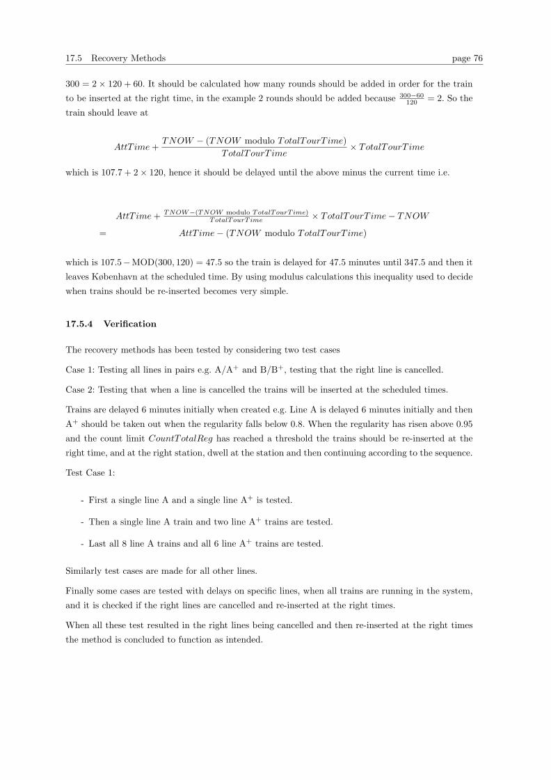
17.5 Recovery Methods page 76
300 = 2× 120 + 60. It should be calculated how many rounds should be added in order for the train
to be inserted at the right time, in the example 2 rounds should be added because 300−60120 = 2. So the
train should leave at
AttT ime +TNOW − (TNOW modulo TotalTourT ime)
TotalTourT ime× TotalTourT ime
which is 107.7 + 2× 120, hence it should be delayed until the above minus the current time i.e.
AttT ime + TNOW−(TNOW modulo TotalTourTime)TotalTourTime × TotalTourT ime− TNOW
= AttT ime− (TNOW modulo TotalTourT ime)
which is 107.5−MOD(300, 120) = 47.5 so the train is delayed for 47.5 minutes until 347.5 and then it
leaves København at the scheduled time. By using modulus calculations this inequality used to decide
when trains should be re-inserted becomes very simple.
17.5.4 Verification
The recovery methods has been tested by considering two test cases
Case 1: Testing all lines in pairs e.g. A/A+ and B/B+, testing that the right line is cancelled.
Case 2: Testing that when a line is cancelled the trains will be inserted at the scheduled times.
Trains are delayed 6 minutes initially when created e.g. Line A is delayed 6 minutes initially and then
A+ should be taken out when the regularity falls below 0.8. When the regularity has risen above 0.95
and the count limit CountTotalReg has reached a threshold the trains should be re-inserted at the
right time, and at the right station, dwell at the station and then continuing according to the sequence.
Test Case 1:
- First a single line A and a single line A+ is tested.
- Then a single line A train and two line A+ trains are tested.
- Last all 8 line A trains and all 6 line A+ trains are tested.
Similarly test cases are made for all other lines.
Finally some cases are tested with delays on specific lines, when all trains are running in the system,
and it is checked if the right lines are cancelled and re-inserted at the right times.
When all these test resulted in the right lines being cancelled and then re-inserted at the right times
the method is concluded to function as intended.
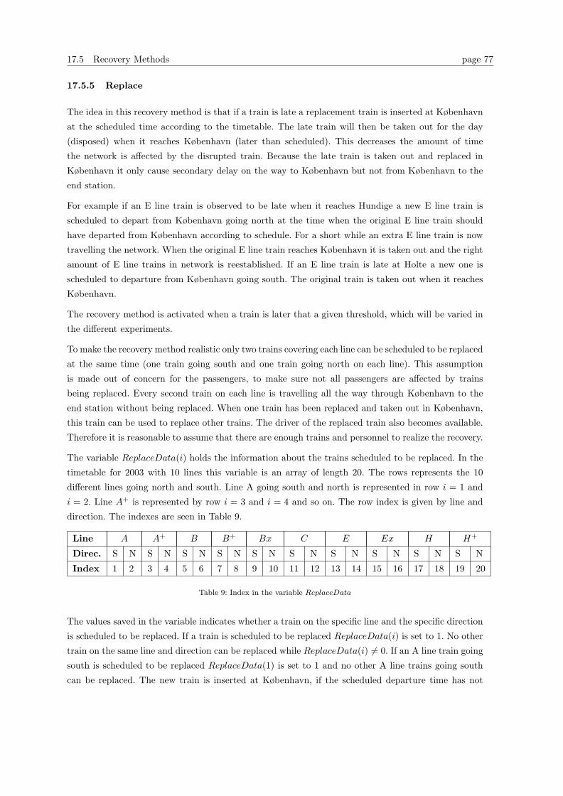
17.5 Recovery Methods page 77
17.5.5 Replace
The idea in this recovery method is that if a train is late a replacement train is inserted at København
at the scheduled time according to the timetable. The late train will then be taken out for the day
(disposed) when it reaches København (later than scheduled). This decreases the amount of time
the network is affected by the disrupted train. Because the late train is taken out and replaced in
København it only cause secondary delay on the way to København but not from København to the
end station.
For example if an E line train is observed to be late when it reaches Hundige a new E line train is
scheduled to depart from København going north at the time when the original E line train should
have departed from København according to schedule. For a short while an extra E line train is now
travelling the network. When the original E line train reaches København it is taken out and the right
amount of E line trains in network is reestablished. If an E line train is late at Holte a new one is
scheduled to departure from København going south. The original train is taken out when it reaches
København.
The recovery method is activated when a train is later that a given threshold, which will be varied in
the different experiments.
To make the recovery method realistic only two trains covering each line can be scheduled to be replaced
at the same time (one train going south and one train going north on each line). This assumption
is made out of concern for the passengers, to make sure not all passengers are affected by trains
being replaced. Every second train on each line is travelling all the way through København to the
end station without being replaced. When one train has been replaced and taken out in København,
this train can be used to replace other trains. The driver of the replaced train also becomes available.
Therefore it is reasonable to assume that there are enough trains and personnel to realize the recovery.
The variable ReplaceData(i) holds the information about the trains scheduled to be replaced. In the
timetable for 2003 with 10 lines this variable is an array of length 20. The rows represents the 10
different lines going north and south. Line A going south and north is represented in row i = 1 and
i = 2. Line A+ is represented by row i = 3 and i = 4 and so on. The row index is given by line and
direction. The indexes are seen in Table 9.
Line A A+ B B+ Bx C E Ex H H+
Direc. S N S N S N S N S N S N S N S N S N S N
Index 1 2 3 4 5 6 7 8 9 10 11 12 13 14 15 16 17 18 19 20
Table 9: Index in the variable ReplaceData
The values saved in the variable indicates whether a train on the specific line and the specific direction
is scheduled to be replaced. If a train is scheduled to be replaced ReplaceData(i) is set to 1. No other
train on the same line and direction can be replaced while ReplaceData(i) 6= 0. If an A line train going
south is scheduled to be replaced ReplaceData(1) is set to 1 and no other A line trains going south
can be replaced. The new train is inserted at København, if the scheduled departure time has not

17.5 Recovery Methods page 78
been exceeded. If the new train is inserted ReplaceData(i) is set to 2, to indicating that the original
train should be taken out, when it reaches København. This is done to make sure the original train
is only taken out if it has been successfully replaced. If a train is scheduled to be replaced at a point
of time later than the time it should depart from København according to the timetable, a new train
cannot be inserted and the original train should not be taken out as planned.
When the original train reaches København and it is not taken out, ReplaceData(i) is set to zero,
to indicating that another train on this line and direction can be replaced if necessary. If the train is
taken out at København ReplaceData is set to zero, 25 minutes later. The reason for this is that only
every second train covering each line in each direction is allowed to be replaced. The interval between
two trains covering the same line is 20 minutes. The 5 minutes represents a buffer, if the next train
should be delayed.
The following pseudo code shows how this recovery method is build in Arena. The method is separated
in two parts. One covering København station where trains are taken out and all other stations where
late trains are observed and scheduled to be inserted at København.
The first pseudo code is for all stations but København, where a train is scheduled to be replaced if
it is later than a given threshold and no other train on the specific line and direction is scheduled to
be replaced. The attributes AttStation, AttT ime and AttStep for the replaced train at København
is calculated in a while loop. The attribute AttDispose is set to 1 to indicate that the train should
be taken out when it reaches København. Finally a new train is created by duplicating the original
one. The attributes are set for the new entity and then it is delayed until it is scheduled to arrive at
København. When the new train is released it enters København station.
if AttStation <> København AND train is late
set row index i for ReplaceData variable % as in the table
if ReplaceData(i) == 0
set AttInsertTime = AttTime
set AttInsertStep = AttStep
while AttInsertStation <> København
AttInsertStep = AttInsertStep + 1
AttStation = Sequence(AttInsertStep,AttLine)
AttInsertTime = AttInsertTime + Dwell(AttStation)+
Running(AttInsertStep,AttLine)
end
set ReplaceData(i) = 1
set AttDispose = 1
set AttStation = Sequence(AttStep,AttLine)
If AttInsertTime > TNOW % The train can be replaced
Duplicate entity
set AttTime = AttInsertTime
set AttStep = AttInsertStep
set ReplaceData(i) = 2
% The original train will be taken out when it reaches København

17.5 Recovery Methods page 79
Delay until AttTime - TNOW
end
end
end
In the pseudo code for the model in København the train entering the station (København) is takenout if it has been successfully replaced.
if AttDispose == 1
if ReplaceData(i) == 2 % the train has been succesfully replaced
Delay 25 minutes
set ReplaceData(i) = 0 % new trains can be replaced
Dispose train/entity
end if
else
set ReplaceData(i) = 0 % new trains can be replaced
AttDispose = 0
end if
17.5.6 Verification
To test the recovery method Replace it is important that the replacement train is inserted at the right
time, that the original train is taken out only if it is replaced and that only one train on each line is
replaced at the same time. The test is split in several cases.
One at a time a train on each line is created and delayed. This train should be replaced at København.
The following values are examined:
- Testing whether the right index i is set for the variable ReplaceData, depending on line and
direction
- Whether ReplaceData(i) is set to one if the train can be replaced and later set to 2 if it is
actually replaced
- See if the new train is inserted at the right time, step and station
- Control that the original train is disposed, but only if it has been replaced
- Make sure that a second train on the same line cannot be replaced before another train has
travelled all the way to København with no interruptions. The following train should not be
replaced but the third train should be allowed to be replaced if necessary
- Ensure that trains later on can get replaced, i.e. ReplaceData(i) is set back to zero 25 minutes
after the train is disposed.
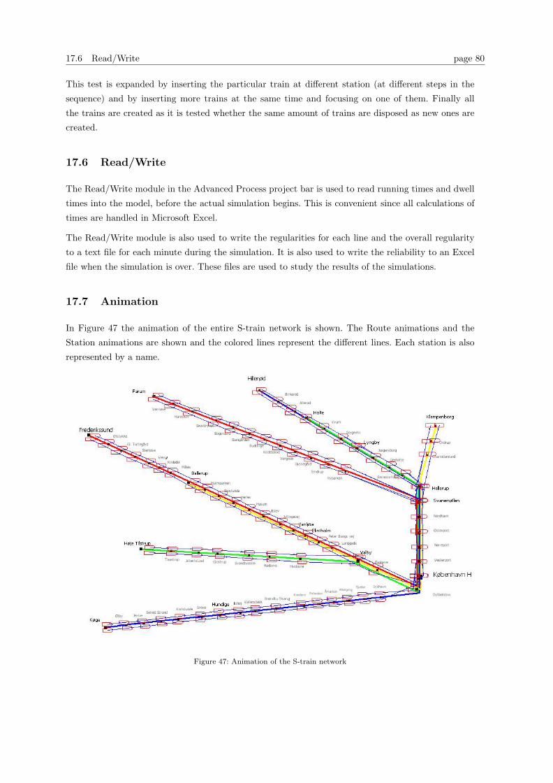
17.6 Read/Write page 80
This test is expanded by inserting the particular train at different station (at different steps in the
sequence) and by inserting more trains at the same time and focusing on one of them. Finally all
the trains are created as it is tested whether the same amount of trains are disposed as new ones are
created.
17.6 Read/Write
The Read/Write module in the Advanced Process project bar is used to read running times and dwell
times into the model, before the actual simulation begins. This is convenient since all calculations of
times are handled in Microsoft Excel.
The Read/Write module is also used to write the regularities for each line and the overall regularity
to a text file for each minute during the simulation. It is also used to write the reliability to an Excel
file when the simulation is over. These files are used to study the results of the simulations.
17.7 Animation
In Figure 47 the animation of the entire S-train network is shown. The Route animations and the
Station animations are shown and the colored lines represent the different lines. Each station is also
represented by a name.
Figure 47: Animation of the S-train network
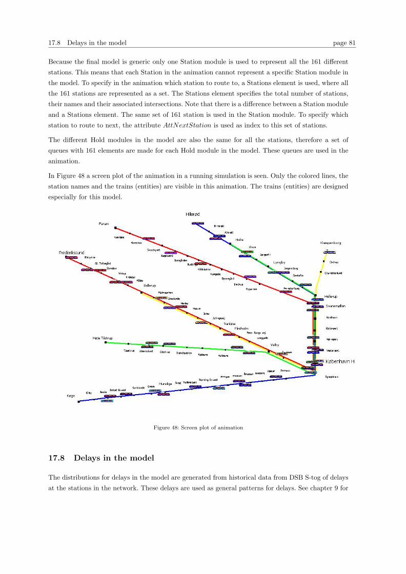
17.8 Delays in the model page 81
Because the final model is generic only one Station module is used to represent all the 161 different
stations. This means that each Station in the animation cannot represent a specific Station module in
the model. To specify in the animation which station to route to, a Stations element is used, where all
the 161 stations are represented as a set. The Stations element specifies the total number of stations,
their names and their associated intersections. Note that there is a difference between a Station module
and a Stations element. The same set of 161 station is used in the Station module. To specify which
station to route to next, the attribute AttNextStation is used as index to this set of stations.
The different Hold modules in the model are also the same for all the stations, therefore a set of
queues with 161 elements are made for each Hold module in the model. These queues are used in the
animation.
In Figure 48 a screen plot of the animation in a running simulation is seen. Only the colored lines, the
station names and the trains (entities) are visible in this animation. The trains (entities) are designed
especially for this model.
Figure 48: Screen plot of animation
17.8 Delays in the model
The distributions for delays in the model are generated from historical data from DSB S-tog of delays
at the stations in the network. These delays are used as general patterns for delays. See chapter 9 for

17.8 Delays in the model page 82
Figure 49: The output from the Input Analyzer
a description of causes of primary delays.
The delays in the historical data are taken from 4 Tuesdays in 2003, distributed over a year to allow for
seasonal changes, and also distributed over the month to allow for daily changes. At DSB S-tog delays
are allowed to be negative (i.e. an early arrival instead of a late arrival). This is not the case in the
model where only actual delays are allowed. Therefore all negative delays are removed. Furthermore
all delays above 2.5 minutes are recorded, hence secondary delays have to be removed before the
distributions can be generated. The number of trains affected by each delay is recorded in the Data
Warehouse at DSB S-tog and these reports can be used to remove all secondary delays manually, since
the first (primary) delay is marked with a code.
The delay data for each station is approximated with a statistical distribution, which is used in the
model. The statistical distributions are found using the Input Analyzer in Arena. The Input Analyzer is
a tool for ´fitting´ statistical distributions to empirical data. The Input Analyzer finds the distribution
best suited for representing the data. It is not necessarily the same type of distribution that fits the
delay data best for all station. It is also possible to fit other distributions instead of the ’best fit’ to
the data, and in this case the Input Analyzer will return the parameters for the chosen distribution
and also the square error when choosing this distribution. The output from the Input Analyzer when
fitting a beta distribution to the delay data for København can be seen in Figure 49.
The beta distribution has been chosen for all the stations in the model, because this was the distribution
18 Verification and validation of the final model page 83
that was returned from the Input Analyzer for the largest number of station. The beta distribution is
also intuitively a fitting choice since the distribution should display a large number of small delays, and
less occurrences of large delay values. This can be achieved with the beta distribution. It could also have
been accomplished by using other distributions. Further more the beta distribution is recommended
to represent delays in the article Test schedule performance and reliability for trains stations [4].
The reason for choosing the beta distribution for all station even though it is not the ’best fit’ in all
cases, is also to get a more homogeneous base for the experiments and as long as the same patterns
of delays are used to evaluate all different timetables, the simulations should give an indication of
the differences between these. In addition the square errors for the beta distributions are rather small
compared to the best fit distributions.
There is a unique distribution for delays at each station, because of the variability in the historical
data. The delays represent primary delays. In appendix H the delay distributions can be seen.
The probability of delays occurring has been fixed at 50% since it turned out that approximately
half of the delays registered in the Data Warehouse at DSB S-tog were negative (i.e. the trains were
arriving early). This is of course a worst case scenario since some negative delays would have cancelled
out some of the the smaller (positive) delays over time.
18 Verification and validation of the final model
It is very important to make sure that the final model runs as intended. Test of the model is separated
in two parts; validation and verification. Validation is the process of ensuring that the model behaves
in the same way as the real system. If the model does not match the real system in all cases it is
important to make some clear assumptions of why the model can be used to simulate the real system.
Verification is the process of ensuring that the final model behave in the way it is intended according
to the modeling assumptions made. This process is also known as debugging.
18.1 Validation and assumptions
One way of validating the model, is to compare it with the real system if such one exists. This was
not possible in this project due to lack of suitable real world results.
Another validation is to study the assumptions made in the modelling phase. The model should be
a representation of the real system except some assumptions that do not affect the credibility of the
model and the results. The degree of assumptions depends on the objective of the simulation project.
The model should be as accurate as possible and match the aim of the given project. Basically the
more accurate the better, but too many detail might in some cases be redundant. The model in this
project is not made to give an exact picture of the real system, but is used to compare timetables
and to see how they differ according to real world scenarios. The most important thing in this project
is that the comparisons are made on the same basis. Because assumptions are made and the model
is not an exact representation of the real network the degree of detail is macroscopic. The following
18.1 Validation and assumptions page 84
assumptions are made:
- The model only simulates worst case scenarios (rush hour). This assumption should not affect
the results since the stability and the robustness of a timetable is assumed lowest in rush hour.
- The trains can never depart earlier than scheduled in the model. This is also considered a worst
case scenario, and does not affect the results.
- Ringbanen is omitted from the model. This change does not have much affect on the results of
the simulation, because Ringbanen is almost a separated network since it only interact with the
other lines in the S-train network at very few stations. In the real system Ringbanen have a very
high regularity and therefore it is excluded in this project.
- In the model all minimum safe headways are set to 1.5 minutes. Actual minimum headways in
the real network are 1.5 minutes in the central area. Other places in the network the actual
minimum safe headways are higher, but exact information could not be obtained and therefore
headways are set to 1.5 minutes in the entire network in the model. This should not have an
impact on the results, since all the timetables are compared on the same basis.
- Possible delays are only added at the stations. The delay follows a distribution made from
historical data. Delays in the real system are added anywhere at the stations or on the routes,
but the historical data is only gathered for each station. The data for a station therefore also
contains the delay on the previous route, which makes this assumption very reasonable.
- The delay added in the model is made from historical data, which makes it very trustworthy.
In the historical data both late and early trains are observed. Since an assumption about trains
never leaving earlier than scheduled are made, the delay distributions are not completely correctly
used in the model. In the model a compensation is made by only adding delay every second time
a train enters a station (delay is added with 50% probability).
- To recover from disruptions (delays) by gaining time is only possible at stations or when turning
around at end stations. This is done by using minimum dwell times and minimum shunting times.
This assumption is very similar to the actual situation, since no data on gaining at routes are
available and trains very rarely gain time while routing between stations, because the scheduled
speed is close to maximum speed.
- In the real system there is only one track between Farum and Værløse, because the track is
crossing an old bridge (Fiskebækbro). This mean that trains in the real system use the same
track in both directions between these two stations. This is not modelled in the simulation model
to simplify the modelling process and because it is mostly in the central area that trains affect
each other.
- Some places in the model the tracks split from one to two tracks or merge from two to one
track. The exact locations of the splits or the merging in the real system are different along the
network. Splitting and merging tracks are implemented in the model in the following way. If the
tracks split or merge between station A and Station B, the tracks split or merge right before the
18.2 Verification page 85
station B. This is done to simplify the model. In the real network, if the tracks are merged right
before station B or split right after station B it is considered the best case scenario because the
tracks are kept double as long as possible. Opposite, if the tracks are merged right after or split
right before station B it is considered the worst case scenario, because this case minimizes the
length of double track. Since both best and worst case scenarios are represented, this assumption
seems reasonable.
- Only the stations existing in the timetable from 2003 is used in all the timetables i.e. the station
Danshøj is omitted. This should have no affect on the simulation, since the running times are
modified to match this case. It is done to be able to compare the results for the different
timetables on the same basis.
- The dwell times used in the timetable from 2003 is used in all the timetables. This does not
affect the simulation, because the running times are calculated from the departure times in the
timetable and the dwell time (running = departure− dwell).
- If data for minimum shunting times were not available they are taken as an average of all
the minimum shunt times. Similarly missing dwell and minimum dwell times are added by
considering the size of the station. This is only the case at very few stations and should not
affect the results.
18.2 Verification
The verification is completed in several phases during the modelling. Every time new modules or
submodels are added it is ensured that the model is running as intended. A lot of the verification is
already done in the previous models build before the final model. In these earlier models it is verified
that all the used flowchart and data modules are used correctly and behave as expected according
to this particular simulation problem. It is further tested whether all the Decide modules split the
entities in the expected directions, that the Hold modules hold the entities until the given condition
is satisfied and that the right assignments are made in the Assign modules. The different expressions
used for actual dwell times, delay and running time are also tested thoroughly in previous models and
in the final model. In Arena it is possible to trace all attribute and variable values and information
about the entities during the simulation, and also to perform the simulation step by step. This has
been used in the verification.
The following is a description of the overall test scenarios.
1. First a very simple verification method is to allow only one single entity to enter the system and
follow that entity step by step to ensure that the model logic is correct.
2. Run the simulation with one line or all lines active to see in the animation whether the right
trains are covering the right lines.
3. For each line verify, that the cycle time (the time it takes to run one round starting at a random
station and ending at the same station) is correct. This test is performed with constant running
18.2 Verification page 86
and dwell times and with added delay and the possibility to gain at stations by using minimum
dwell times or by gaining at the end station by using minimum shunting time. This verifies that
the running and dwell times are correct and that the trains can gain time correctly at stations
and while shunting at the end station.
4. Verify that the trains on all lines are stopping at the right stations. Also that the dwell and
running times are correct according to the timetable. This is done by sending one train through
the system and then examine the output file to verify the stopping pattern, the dwell times and
the running times. This is repeated for all the lines.
By making these four test in the given order small errors are found in the first cases. The last case is
more time consuming but the only one that verifies the model in details.
19 Development of timetables for experiments page 87
19 Development of timetables for experiments
When experimenting with robustness in timetables several timetables with different features are neces-
sary. Different features are number of lines, stopping patterns, line structure, cycle time, homogeneous
use of the double tracks, homogeneous scheduled headways and buffer times at end stations. Each
timetable used in the experiments in this project has some of these specific characteristics which all
relate to robustness and customer service level. In all the timetables every line are departing with a
frequency of 20 minutes. The timetables are partly developed by DSB S-tog and partly constructed
for this project. The overall timetables used in the experiments are:
- Actual timetable for 2006 (9 lines) developed by DSB S-tog
- Actual timetable from 2003 (10 lines) developed by DSB S-tog
- Proposed timetable with 10 lines developed by DSB S-tog
- Proposed timetable with 11 lines partly developed by DSB S-tog
- Proposed timetable with 12 lines partly developed by DSB S-tog
- Constructed timetable with 20 lines including a circular line in the central section
- Constructed timetable with 17 lines and a combination of circular line and drive-through lines
in the central section.
These timetables and modifications of them will be examined thoroughly in the following sections. All
the modifications are made specifically for this project.
19.0.1 Timetable from 2003
The actual timetable for 2003 with 10 lines is developed by DSB S-tog and was used in 2003. It is
very similar to the normal timetable in 2005. The timetable for 2003 is included in the experiments
to analyse the current situation. This timetable was the first data received from DSB S-tog and the
Arena model is build based on this timetable. The line plan of the 2003 timetable is shown in Figure
50.
In the real system line Ex is inserted in Køge, drive to Hellerup and is taken out at København. A
version of the timetable from 2003 has been developed where line Ex is taken out in København, to
examine the situation in the real world system.
In the general plan from 2003 used in this project line Ex is augmented from København to Køge
to make line Ex circular. In reality only four departures for line Ex exist during the day. These four
departures are in the morning rush hour. In this project line Ex is run continually, because the purpose
is to examine a worst case situation.
A version of the 2003 timetable with a more homogeneous distribution of the tracks at København
has also been developed and implemented. In København there are two tracks in each direction. The
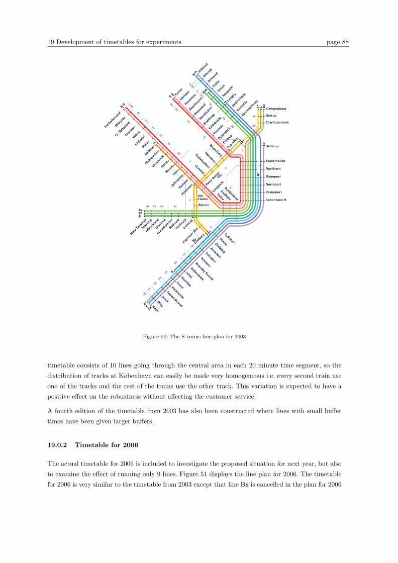
19 Development of timetables for experiments page 88
66 54 43 32
20
99
89
77
67
55
44
33
2
82
7161
51
41
30
62
52
41
31
94
85
74
63
53
42
31
2
7
9
1
40
30
2
2
2
København H
Sydhavn
Peter
Ban
gsVej
SjælørEllebjerg
Åmarken
FrihedenAvedøre
Brøndby Strand
Vallensbæk
IshøjHundigeGreveKarlslunde
Solrød Strand
JersieØlbyKøge
Berns
torff
svej
Gento
fteJæ
gers
borg
Lyng
bySorg
enfri
VirumHolteBirk
erød
Allerø
dHiller
ød
Rødovre
Brønd
byøst
er
Glost
rup
Alber
tslu
nd
Taas
trup
Høje Ta
astru
p
Vesterport
Nørreport
Nordhavn
Svanemøllen
Hellerup
Charlottenlund
Ordrup
Klampenborg
Emdru
p
Rypar
kenDys
segå
rd
Vange
deKild
ebak
ke
Buddinge
Sten
gård
en
Bagsv
ærd
Skovb
ryne
t
Hares
kov
Værlø
seFaru
m
Bispebjerg
Valby
Enghave
Dybbølsbro
Vanlø
se
Jylli
ngev
ejIsle
vHusumHer
lev
Skovl
unde
Mal
mpar
ken
Balle
rupM
åløv
Kilded
alVeksø
Lang
gade
Sten
løse
Ølst
ykke
Gl. To
ftegå
rd
Hvidovr
e
Østerport
Fred
erik
ssund
Flin
tholm
Nørrebro
FuglebakkenGrøndal
Dansh
øj
KBHallen
Ålholm
Viger
slev
Allé
NyEl
lebje
rg
C
H +
EA
BB +
H
F+
C
BxB+B
A+
E
Ex
A
A+E
H +H
F
Ex
FF+
Bx
F+
DSB S-togKøreplan Gælder fra januar 2005
Figure 50: The S-trains line plan for 2003
timetable consists of 10 lines going through the central area in each 20 minute time segment, so the
distribution of tracks at København can easily be made very homogeneous i.e. every second train use
one of the tracks and the rest of the trains use the other track. This variation is expected to have a
positive effect on the robustness without affecting the customer service.
A fourth edition of the timetable from 2003 has also been constructed where lines with small buffer
times have been given larger buffers.
19.0.2 Timetable for 2006
The actual timetable for 2006 is included to investigate the proposed situation for next year, but also
to examine the effect of running only 9 lines. Figure 51 displays the line plan for 2006. The timetable
for 2006 is very similar to the timetable from 2003 except that line Bx is cancelled in the plan for 2006
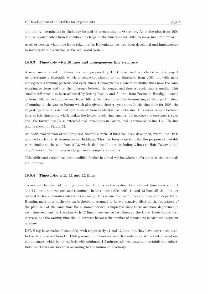
19 Development of timetables for experiments page 89
and line A+ terminates in Buddinge instead of terminating at Østerport. As in the plan from 2003
line Ex is augmented from København to Køge in the timetable for 2006, to make line Ex circular.
Another version where line Ex is taken out in København has also been developed and implemented
to investigate the situation in the real world system.
19.0.3 Timetable with 10 lines and homogeneous line structure
A new timetable with 10 lines has been proposed by DSB S-tog, and is included in this project
to investigate a timetable which is somewhat similar to the timetable from 2003 but with more
homogeneous running patterns and cycle times. Homogeneous means that similar lines have the same
stopping patterns and that the difference between the longest and shortest cycle time is smaller. This
smaller difference has been achieved by letting lines A and A+ run from Farum to Hundige, instead
of from Hillerød to Hundige and from Hillerød to Køge. Line H is terminating at Østerport instead
of running all the way to Farum which also gives a shorter cycle time. In the timetable for 2003, the
longest cycle time is defined by the series from Frederikssund to Farum. This series is split between
lines in this timetable, which makes the longest cycle time smaller. To improve the customer service
level the former line Bx is extended and terminates in Farum, and is renamed to line Dx. The line
plan is shown in Figure 52.
An additional version of the proposed timetable with 10 lines has been developed, where line Dx is
modified such that it terminates in Buddinge. This has been done to make the proposed timetable
more similar to the plan from 2003, which also has 10 lines, including 3 lines to Høje Taastrup and
only 2 lines to Farum, to possibly get more comparable results.
This additional version has been modified further in a final version where buffer times at the terminals
are improved.
19.0.4 Timetables with 11 and 12 lines
To analyse the effect of running more than 10 lines in the system, two different timetables with 11
and 12 lines are developed and examined. In these timetables with 11 and 12 lines all the lines are
covered with a 20 minutes interval as normally. This means that more lines result in more departures.
Running more lines in the system is therefore assumed to have a negative effect on the robustness of
the plan, but at the same time the customer service is improved since there are more departures in
each time segment. In the plan with 12 lines there are no fast lines, so the travel times should also
increase, but the waiting time should decrease because the number of departures in each time segment
increase.
DSB S-tog have drafts of timetables with respectively 11 and 12 lines, but they have never been used.
In the data received from DSB S-tog some of the lines arrive at København (and the central area) one
minute apart, which is not realistic with minimum 1.5 minute safe headways and certainly not robust.
Both timetables are modified according to the minimum headways.
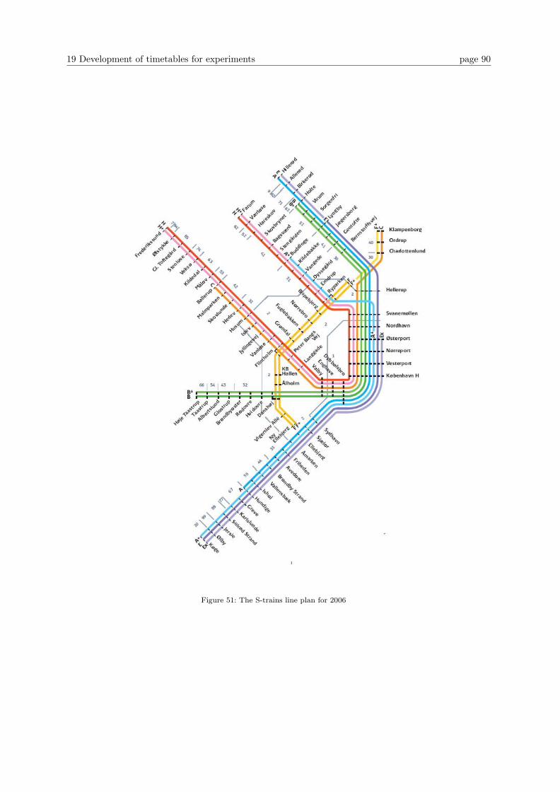
19 Development of timetables for experiments page 90
Figure 51: The S-trains line plan for 2006

19 Development of timetables for experiments page 91
København H
Sydhavn
Peter
Ban
gs
Vej
SjælørN
y Ellebjerg
Åmarken
FrihedenAvedøre
Brøndby Strand
Vallensbæk
IshøjHundigeGreveKarlslunde
Solrød Strand
JersieØlbyKøge
Berns
torff
svej
Gento
fteJæ
gers
borg
Lyng
bySorg
enfri
VirumHolteBirk
erød
Allerø
dHiller
ød
Rødovre
Brønd
byøst
er
Glost
rup
Alber
tslu
nd
Taas
trup
Høje T
aast
rup
Vesterport
Nørreport
Nordhavn
Svanemøllen
Hellerup
Charlottenlund
Ordrup
Klampenborg
Emdru
p
Rypar
kenDys
segå
rd
Vange
deKild
ebak
ke
Buddinge
Sten
gård
en
Bagsv
ærd
Skovb
ryne
t
Hares
kov
Værlø
seFaru
m
Bispebjerg
Valby
Enghave
Dybbølsbro
Vanlø
se
Jylli
ngev
ejIsl
evHusumHer
lev
Skovl
unde
Mal
mpar
ken
Balle
rupM
åløv
Kilded
alVeksø
Lang
gade
Sten
løse
Ølst
ykke
Gl. To
ftegå
rd
Hvidovr
e
Østerport
Fred
erik
ssund
Flin
tholm
Nørrebro
FuglebakkenGrøndal
Dansh
øj
KBHallen
Ålholm
Viger
slev
Allé
Dx
E+
E
D+
F
E
A +
B +
C+
B+
A+
C
/D+
FC +
E +
D+
R +
R+
Dx
E +
A +
B+
B+
A+
C +
Dx
E+
C+
R+
R +
R
BA
B
A
F
C
E
C
F
E
R
S2006Hurtigløsning Myldretider
Figure 52: The proposed line plan with 10 lines
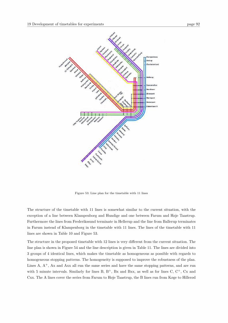
19 Development of timetables for experiments page 92
Figure 53: Line plan for the timetable with 11 lines
The structure of the timetable with 11 lines is somewhat similar to the current situation, with the
exception of a line between Klampenborg and Hundige and one between Farum and Høje Taastrup.
Furthermore the lines from Frederikssund terminate in Hellerup and the line from Ballerup terminates
in Farum instead of Klampenborg in the timetable with 11 lines. The lines of the timetable with 11
lines are shown in Table 10 and Figure 53.
The structure in the proposed timetable with 12 lines is very different from the current situation. The
line plan is shown in Figure 54 and the line description is given in Table 11. The lines are divided into
3 groups of 4 identical lines, which makes the timetable as homogeneous as possible with regards to
homogeneous stopping patterns. The homogeneity is supposed to improve the robustness of the plan.
Lines A, A+, Ax and Axx all run the same series and have the same stopping patterns, and are run
with 5 minute intervals. Similarly for lines B, B+, Bx and Bxx, as well as for lines C, C+, Cx and
Cxx. The A lines cover the series from Farum to Høje Taastrup, the B lines run from Køge to Hillerød
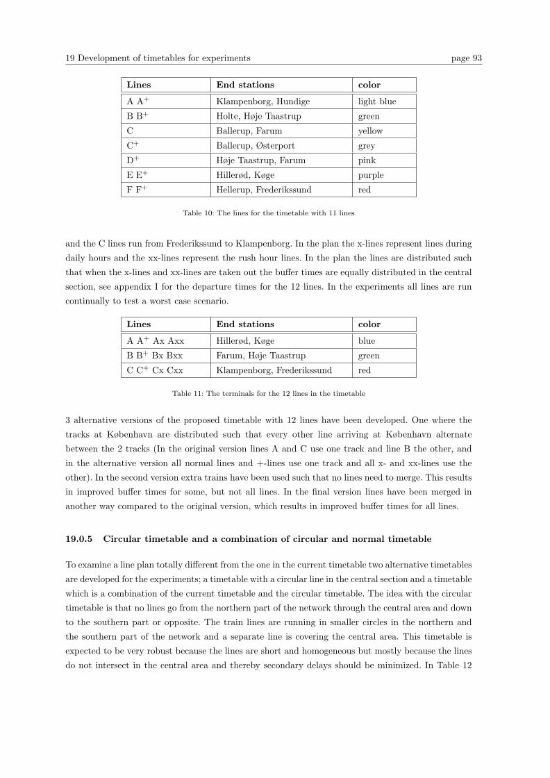
19 Development of timetables for experiments page 93
Lines End stations color
A A+ Klampenborg, Hundige light blue
B B+ Holte, Høje Taastrup green
C Ballerup, Farum yellow
C+ Ballerup, Østerport grey
D+ Høje Taastrup, Farum pink
E E+ Hillerød, Køge purple
F F+ Hellerup, Frederikssund red
Table 10: The lines for the timetable with 11 lines
and the C lines run from Frederikssund to Klampenborg. In the plan the x-lines represent lines during
daily hours and the xx-lines represent the rush hour lines. In the plan the lines are distributed such
that when the x-lines and xx-lines are taken out the buffer times are equally distributed in the central
section, see appendix I for the departure times for the 12 lines. In the experiments all lines are run
continually to test a worst case scenario.
Lines End stations color
A A+ Ax Axx Hillerød, Køge blue
B B+ Bx Bxx Farum, Høje Taastrup green
C C+ Cx Cxx Klampenborg, Frederikssund red
Table 11: The terminals for the 12 lines in the timetable
3 alternative versions of the proposed timetable with 12 lines have been developed. One where the
tracks at København are distributed such that every other line arriving at København alternate
between the 2 tracks (In the original version lines A and C use one track and line B the other, and
in the alternative version all normal lines and +-lines use one track and all x- and xx-lines use the
other). In the second version extra trains have been used such that no lines need to merge. This results
in improved buffer times for some, but not all lines. In the final version lines have been merged in
another way compared to the original version, which results in improved buffer times for all lines.
19.0.5 Circular timetable and a combination of circular and normal timetable
To examine a line plan totally different from the one in the current timetable two alternative timetables
are developed for the experiments; a timetable with a circular line in the central section and a timetable
which is a combination of the current timetable and the circular timetable. The idea with the circular
timetable is that no lines go from the northern part of the network through the central area and down
to the southern part or opposite. The train lines are running in smaller circles in the northern and
the southern part of the network and a separate line is covering the central area. This timetable is
expected to be very robust because the lines are short and homogeneous but mostly because the lines
do not intersect in the central area and thereby secondary delays should be minimized. In Table 12
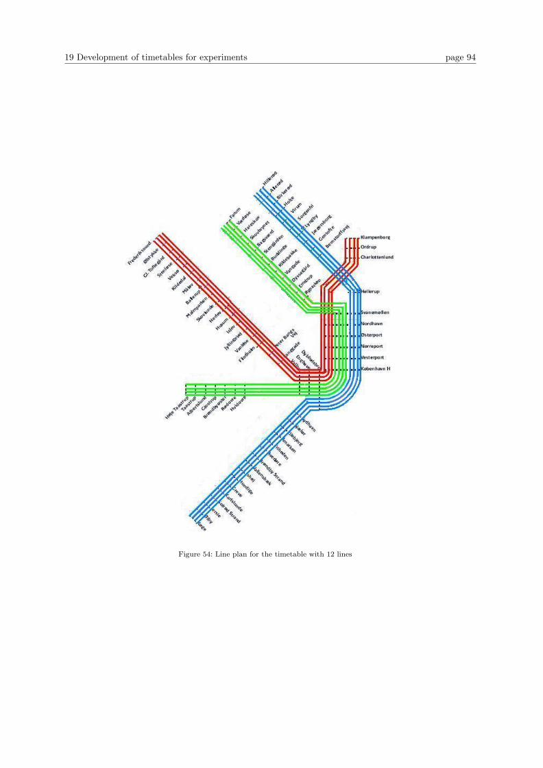
19 Development of timetables for experiments page 94
Figure 54: Line plan for the timetable with 12 lines
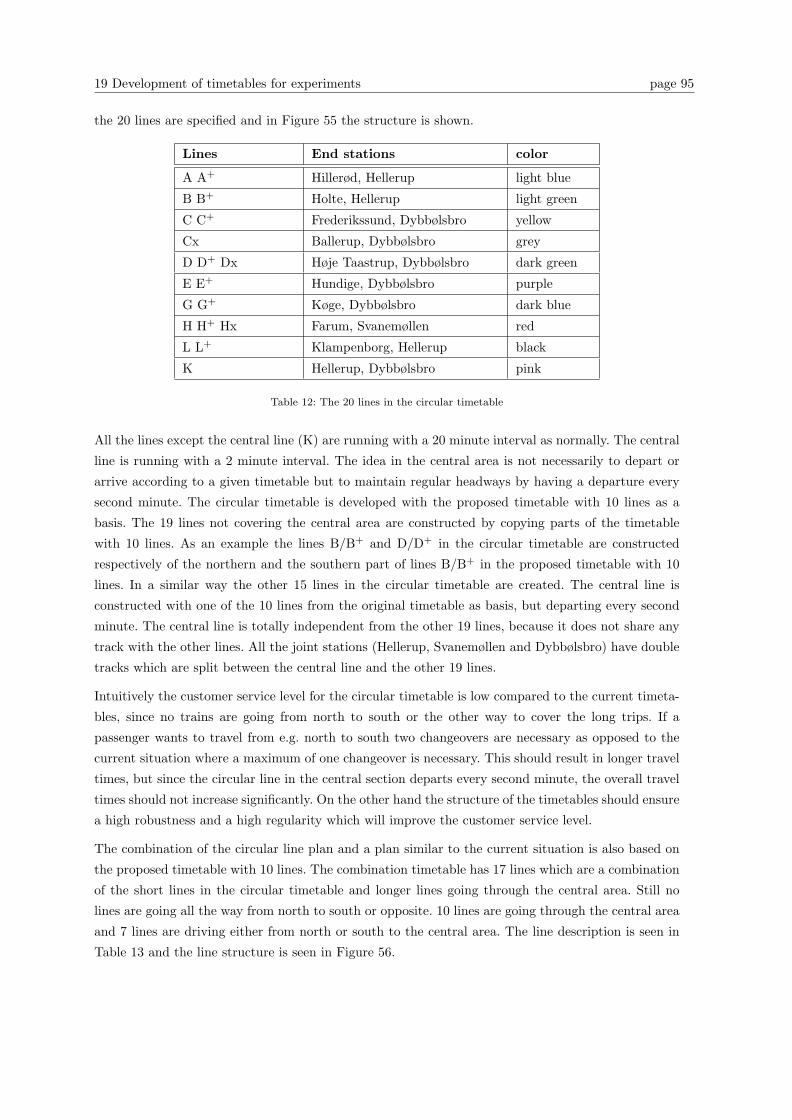
19 Development of timetables for experiments page 95
the 20 lines are specified and in Figure 55 the structure is shown.
Lines End stations color
A A+ Hillerød, Hellerup light blue
B B+ Holte, Hellerup light green
C C+ Frederikssund, Dybbølsbro yellow
Cx Ballerup, Dybbølsbro grey
D D+ Dx Høje Taastrup, Dybbølsbro dark green
E E+ Hundige, Dybbølsbro purple
G G+ Køge, Dybbølsbro dark blue
H H+ Hx Farum, Svanemøllen red
L L+ Klampenborg, Hellerup black
K Hellerup, Dybbølsbro pink
Table 12: The 20 lines in the circular timetable
All the lines except the central line (K) are running with a 20 minute interval as normally. The central
line is running with a 2 minute interval. The idea in the central area is not necessarily to depart or
arrive according to a given timetable but to maintain regular headways by having a departure every
second minute. The circular timetable is developed with the proposed timetable with 10 lines as a
basis. The 19 lines not covering the central area are constructed by copying parts of the timetable
with 10 lines. As an example the lines B/B+ and D/D+ in the circular timetable are constructed
respectively of the northern and the southern part of lines B/B+ in the proposed timetable with 10
lines. In a similar way the other 15 lines in the circular timetable are created. The central line is
constructed with one of the 10 lines from the original timetable as basis, but departing every second
minute. The central line is totally independent from the other 19 lines, because it does not share any
track with the other lines. All the joint stations (Hellerup, Svanemøllen and Dybbølsbro) have double
tracks which are split between the central line and the other 19 lines.
Intuitively the customer service level for the circular timetable is low compared to the current timeta-
bles, since no trains are going from north to south or the other way to cover the long trips. If a
passenger wants to travel from e.g. north to south two changeovers are necessary as opposed to the
current situation where a maximum of one changeover is necessary. This should result in longer travel
times, but since the circular line in the central section departs every second minute, the overall travel
times should not increase significantly. On the other hand the structure of the timetables should ensure
a high robustness and a high regularity which will improve the customer service level.
The combination of the circular line plan and a plan similar to the current situation is also based on
the proposed timetable with 10 lines. The combination timetable has 17 lines which are a combination
of the short lines in the circular timetable and longer lines going through the central area. Still no
lines are going all the way from north to south or opposite. 10 lines are going through the central area
and 7 lines are driving either from north or south to the central area. The line description is seen in
Table 13 and the line structure is seen in Figure 56.
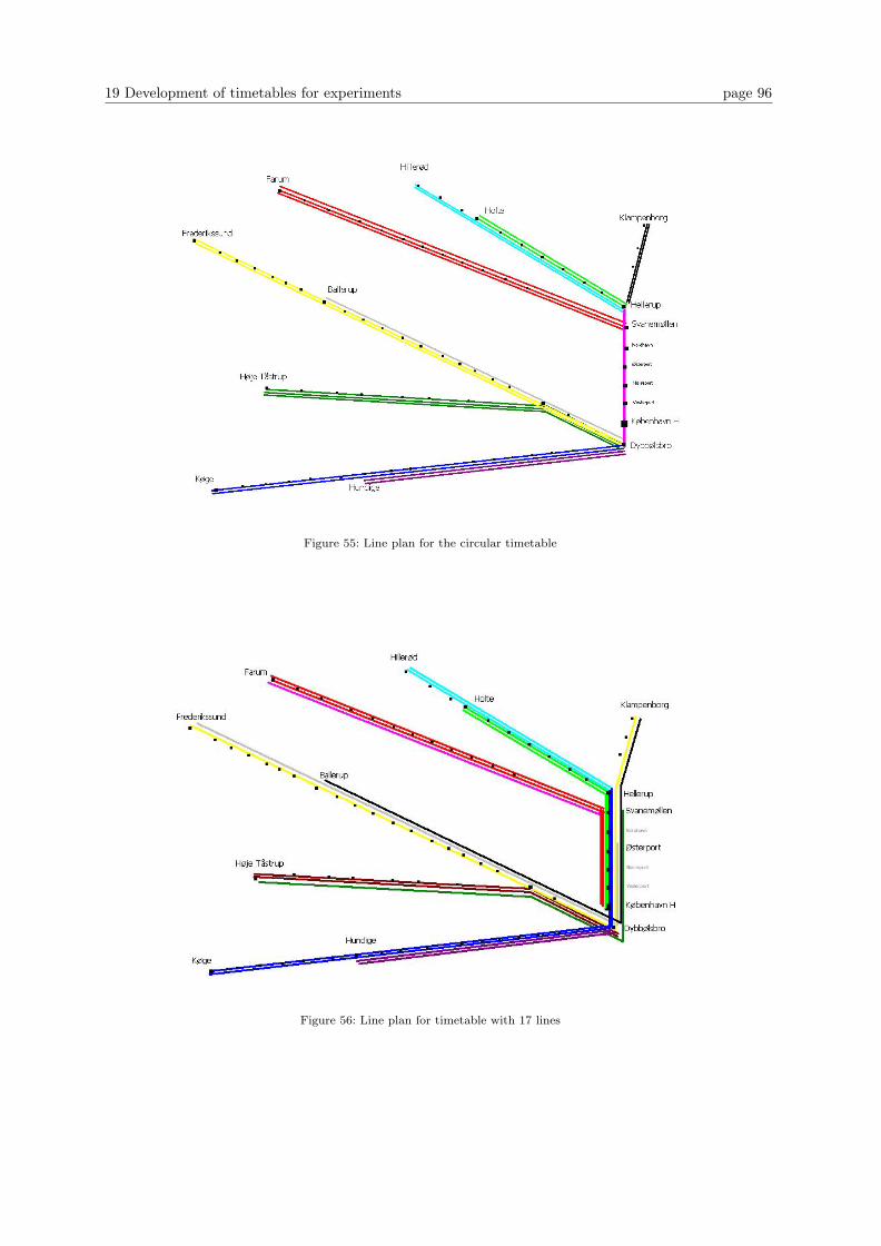
19 Development of timetables for experiments page 96
Figure 55: Line plan for the circular timetable
Figure 56: Line plan for timetable with 17 lines
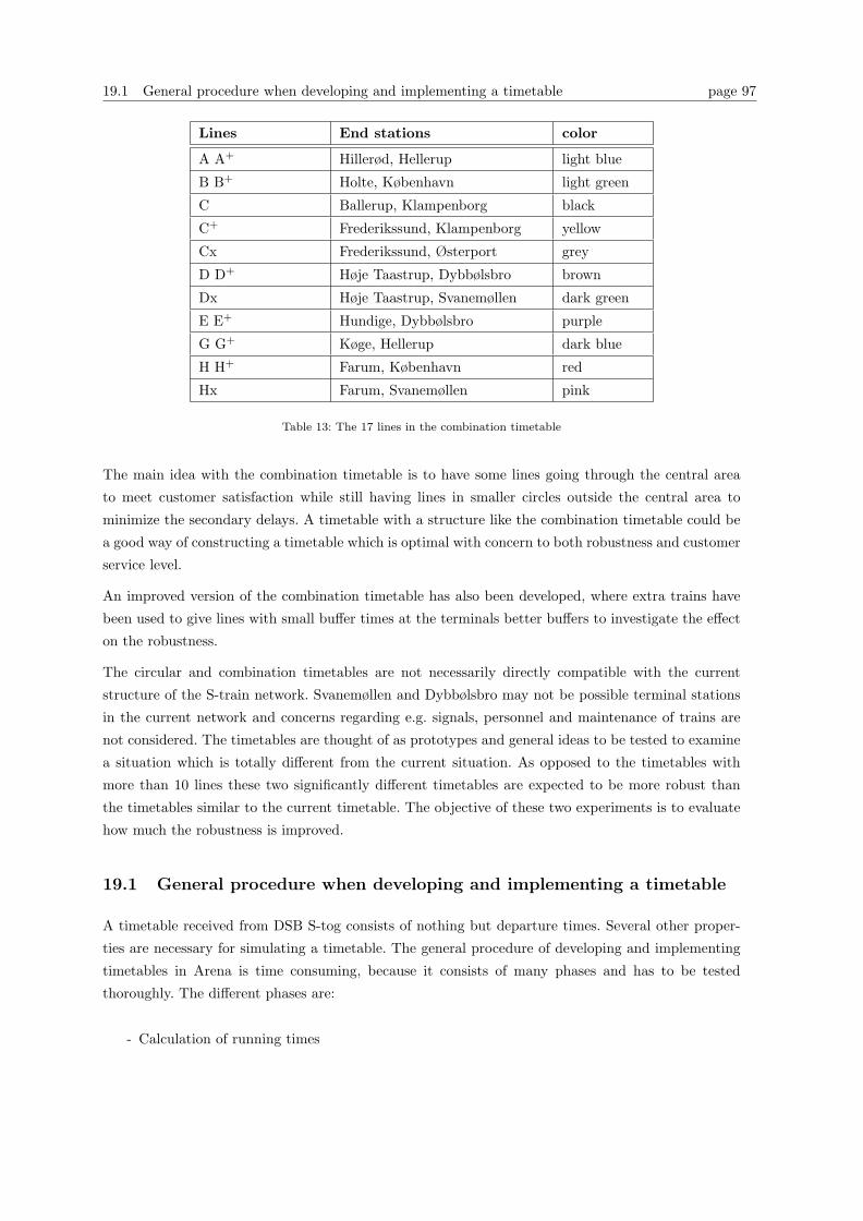
19.1 General procedure when developing and implementing a timetable page 97
Lines End stations color
A A+ Hillerød, Hellerup light blue
B B+ Holte, København light green
C Ballerup, Klampenborg black
C+ Frederikssund, Klampenborg yellow
Cx Frederikssund, Østerport grey
D D+ Høje Taastrup, Dybbølsbro brown
Dx Høje Taastrup, Svanemøllen dark green
E E+ Hundige, Dybbølsbro purple
G G+ Køge, Hellerup dark blue
H H+ Farum, København red
Hx Farum, Svanemøllen pink
Table 13: The 17 lines in the combination timetable
The main idea with the combination timetable is to have some lines going through the central area
to meet customer satisfaction while still having lines in smaller circles outside the central area to
minimize the secondary delays. A timetable with a structure like the combination timetable could be
a good way of constructing a timetable which is optimal with concern to both robustness and customer
service level.
An improved version of the combination timetable has also been developed, where extra trains have
been used to give lines with small buffer times at the terminals better buffers to investigate the effect
on the robustness.
The circular and combination timetables are not necessarily directly compatible with the current
structure of the S-train network. Svanemøllen and Dybbølsbro may not be possible terminal stations
in the current network and concerns regarding e.g. signals, personnel and maintenance of trains are
not considered. The timetables are thought of as prototypes and general ideas to be tested to examine
a situation which is totally different from the current situation. As opposed to the timetables with
more than 10 lines these two significantly different timetables are expected to be more robust than
the timetables similar to the current timetable. The objective of these two experiments is to evaluate
how much the robustness is improved.
19.1 General procedure when developing and implementing a timetable
A timetable received from DSB S-tog consists of nothing but departure times. Several other proper-
ties are necessary for simulating a timetable. The general procedure of developing and implementing
timetables in Arena is time consuming, because it consists of many phases and has to be tested
thoroughly. The different phases are:
- Calculation of running times
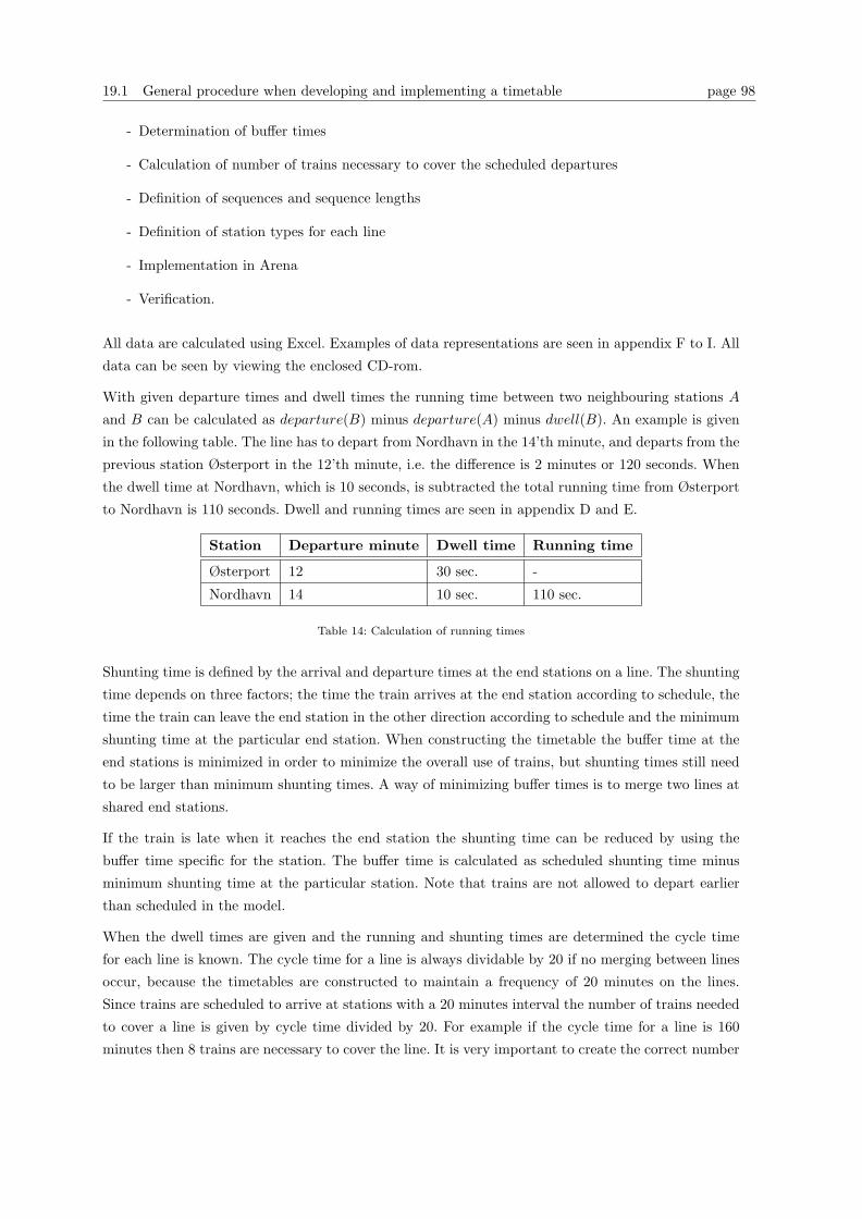
19.1 General procedure when developing and implementing a timetable page 98
- Determination of buffer times
- Calculation of number of trains necessary to cover the scheduled departures
- Definition of sequences and sequence lengths
- Definition of station types for each line
- Implementation in Arena
- Verification.
All data are calculated using Excel. Examples of data representations are seen in appendix F to I. All
data can be seen by viewing the enclosed CD-rom.
With given departure times and dwell times the running time between two neighbouring stations A
and B can be calculated as departure(B) minus departure(A) minus dwell(B). An example is given
in the following table. The line has to depart from Nordhavn in the 14’th minute, and departs from the
previous station Østerport in the 12’th minute, i.e. the difference is 2 minutes or 120 seconds. When
the dwell time at Nordhavn, which is 10 seconds, is subtracted the total running time from Østerport
to Nordhavn is 110 seconds. Dwell and running times are seen in appendix D and E.
Station Departure minute Dwell time Running time
Østerport 12 30 sec. -
Nordhavn 14 10 sec. 110 sec.
Table 14: Calculation of running times
Shunting time is defined by the arrival and departure times at the end stations on a line. The shunting
time depends on three factors; the time the train arrives at the end station according to schedule, the
time the train can leave the end station in the other direction according to schedule and the minimum
shunting time at the particular end station. When constructing the timetable the buffer time at the
end stations is minimized in order to minimize the overall use of trains, but shunting times still need
to be larger than minimum shunting times. A way of minimizing buffer times is to merge two lines at
shared end stations.
If the train is late when it reaches the end station the shunting time can be reduced by using the
buffer time specific for the station. The buffer time is calculated as scheduled shunting time minus
minimum shunting time at the particular station. Note that trains are not allowed to depart earlier
than scheduled in the model.
When the dwell times are given and the running and shunting times are determined the cycle time
for each line is known. The cycle time for a line is always dividable by 20 if no merging between lines
occur, because the timetables are constructed to maintain a frequency of 20 minutes on the lines.
Since trains are scheduled to arrive at stations with a 20 minutes interval the number of trains needed
to cover a line is given by cycle time divided by 20. For example if the cycle time for a line is 160
minutes then 8 trains are necessary to cover the line. It is very important to create the correct number

19.1 General procedure when developing and implementing a timetable page 99
of trains for each line. If a smaller number of trains are created a gap of more than 20 minutes between
the first and the last inserted train will exist. Opposite if more trains than needed are inserted the
first and the last inserted train will arrive at stations at the same time, which is not permitted. In the
case where two lines are merging the cycle time may not be dividable by 20, but by 10. The B and
B+-trains are merged e.g. in the timetable used in 2003. The cycle time is 130 minutes for both lines
which results in 6 B-trains and 7 B+-trains or 7 B-trains and 6 B+-trains needed.
For each line in the timetable a sequence of stations is defined. A sequence for a specific line is all
the stations the train covering that line is passing (stopping or not). An example of a sequences is
seen in appendix G. The sequence length is the number of stations in a sequence. The double tracks
at some stations are distributed between all the train lines. The distribution of the double tracks is
done according to the line structures, e.g. the double tracks at Dybbølsbro station in the northern
direction is split between the lines from Sydhavn and the lines coming from Enghave. Similarly with
the double tracks at Valby north, Hellerup and Svanemøllen. The distribution of the double tracks
at København is different. Because all the lines have the same conditions at this station, no natural
splitting exists. The double tracks at København can be split to obtain maximal headways at both
track or with concern of customer satisfaction i.e. letting similar lines such as A/A+ use the same
track/platforms.
To specify whether a line is scheduled to stop at a particular station in the sequence, station types
specific for each line are defined. The station type is set to 1 to specify that the line is scheduled to
stop on this particular station, and 3 if not. Station type 2 indicates the end stations for the particular
line. The running time can only be reduced at the end stations, therefore a specific station type for
end stations is used. In appendix F an example of station types is shown.
Implementing a new timetable in Arena requires that many of the variables are changed according to
value and dimension. The values depend on the timetable and the dimensions mostly depend on the
number of lines or sequence lengths. The new values (running times, sequences etc.) are either read
directly from Excel when the simulation is running or copied manually. In addition some modules in
the model should be changed or added to match the timetable. Other amounts of trains might be
necessary to cover the lines, depending on the cycle times for the lines and the number of lines. If
lines are merged this feature must also be adjusted in the model. Finally the recovery methods must
be adapted to match the new timetable.
Finally the Arena model matching the new timetable is tested thoroughly to verify that it is running
as intended. This is done by repeating the tests of the entire final model and parts of the tests of the
recovery methods.

20 Experiments page 100
20 Experiments
In the following chapters the experiments with the different timetables are presented and analyzed. The
timetables are described in chapter 19. Experiments will be made with the main timetables and with
the modified versions. The experiments concern evaluation of the recovery methods and comparison
of the timetables. Furthermore the following hypotheses will be examined throughout these chapters.
- Secondary delays have a significant negative effect on regularity.
- Average delay and regularity are linearly dependent.
- Larger buffers at the end stations have a positive effect on regularity and robustness.
- A more homogeneous timetable with regards to stopping patterns, will result in a higher robust-
ness.
- Even distribution of the tracks on København station will result in more robust timetables.
- More lines in a timetable result in a lower regularity.
- A timetable with 12 lines and a frequency of 20 minutes will increase the customer service level
and might be possible without decreasing the stability of the system.
- A new network pattern where lines are split into northern lines, southern lines and shuttle service
in the central part of the network will result in a more robust timetable (circular timetable).
- A timetable similar to the circular timetable, but with some lines running through the central
section before turning, called the combination timetable, will result in higher regularity.
In this chapter some introductions to fundamental conditions for the experiment are given. In chapter
21 the results from the experiments with the individual timetables are reviewed. All the different
timetables are simulated with and without use of recovery methods. In chapter 21 the main objective
is to examine the effect of the three recovery methods on the different timetables. Chapter 22 presents
the results from additional experiments with delay and with buffer time at the end stations. In chapter
23 all the different timetables are compared. The main objective of chapter 23 is to examine what
effect more lines, different line structures and buffer time have on regularity and robustness. Finally
in chapter 24 overall conclusions on all the experiment will be given. The results that are evaluated
but not presented in the chapters are given in appendix J.
20.1 Introduction
All experiments will be run for 12.5 hours from 6:00 to 18:30 i.e. 750 minutes, since this is approximately
the period of time when all lines (except x-lines) are running in the network in the real system. Due
to the insertion time of all the trains, the simulation time will actually be 1000 minutes. There is a
250 minute warm up period before all trains are actually running in the system. All lines will be run
20.1 Introduction page 101
continually, even though the x-lines are cancelled outside rush hour in the real world situation. This
is done to test the worst case robustness of the different plans. Note that the simulation time is in
minutes, i.e. when referring to ’time’ in the experiments or in figures, the unit is minutes. In the results
from the experiments the warm up period is never considered. This means that regularity, reliability
and average delay are measured after the warm up period. Furthermore the time on the x-axes in
figures starting at 0 minutes is after the warm up period of 250 minutes.
In section 17.8 it is described how delay for each stations is calculated from historical data. Delay
for each station is given by a distribution. In the experiments there will be 50% probability of delays
occurring at each station. 50% probability of delays means that approximately every second time a
train enters a station, delay is added according to the distribution of delay for the particular station.
As explained delays are drawn from a distribution and therefore 5 independent statistically identical
simulations are run, to reduce the effect of outlying random values. An experiment with 10 replica-
tions was made and there were no considerable differences in the mean values, therefore 5 replications
is considered sufficient. Only the mean value taken from the 5 replications is considered in the ex-
periments. Mean regularity, mean reliability and average delay occurring for the trains are recorded
for each experiment. In experiments with recovery methods the numbers of affected trains are also
recorded. These values might be non-integral since they are average values from the 5 replications.
To broaden the level of comparison in the experiments the timetables are simulated with and without
use of recovery method. The test cases for each timetable are:
1. With delays, but without recovery
2. With delays and recovery method Take out
3. With delays and recovery method Turn around
4. With delays and recovery method Replace.
In the experiments the following measures of robustness are used:
1. Regularity (percentage of trains running on time)
2. Average delay
3. Reliability (number of planned departures compared to actual number of departures)
4. Number of affected trains (replaced, turned or cancelled).
In principle high robustness is indicated by a stable regularity. Furthermore in this context high
regularity indicates high robustness. A high regularity and few affected trains also indicates high
robustness.
20.2 Fundamental conditions for the experiments page 102
20.2 Fundamental conditions for the experiments
The data used for the experiments consists of several timetables with different features. Using simula-
tion these different timetables can be compared with respect to robustness, but many factors should
be considered while making this comparison.
The number of lines is an important factor when examining the robustness of a timetable, but there
are also other factors which should be considered. Number of trains necessary for running the plan
and buffer times at the end stations have a big influence on robustness. In Table 15 the minimum,
maximum and average buffer times (in minutes) at the end stations and the trains needed to cover the
scheduled departures in the timetable are listed for the different timetables. A timetable is assumed
robust if it has large average buffer times at the terminal stations, but larger buffer times at terminal
stations results in a larger number of trains necessary to cover the timetable. Seen from an economical
point of view the fewer trains needed the better. The optimal solution is a robust timetable with as
few trains as possible.
Some of the timetables constructed by DSB S-tog are made with different running times, because
new trains have made it possible to run faster. With faster running times fewer trains can cover the
timetable. This makes the possibility of comparing timetables according to necessary number of trains
somewhat more difficult. An exact comparison on the basis of number of trains needed is therefore
only possible when modifications of the particular timetables are made.
In the results it should be accounted for that not all lines have the same departure times in each plan.
Therefore some variability can occur in the results even though two timetables seem to be similar. As
an example the line Ex has different departure times in the plan for 2003 (10 lines) and 2006 (9 lines),
which results in line Ex departing from København differently for each of the two timetables, which
again results in line Ex following lines E and A+ respectively on the route from København to Køge.
In this example line Ex is affected by secondary delays from different trains which has an effect on the
overall robustness. Generally the construction of the timetables has a big influence on the robustness.
The order of the lines in the central area where most secondary delay occur is different from plan to
plan and therefore complicates the comparison.
The main problem when comparing the different timetables is that only one or two of each type
(number of lines or structure) are represented in the experiments. This makes the basis of comparison
more uncertain and the possibility of generalizing the results difficult, but it is still possible to give an
overall comparison by taking these issues into consideration.
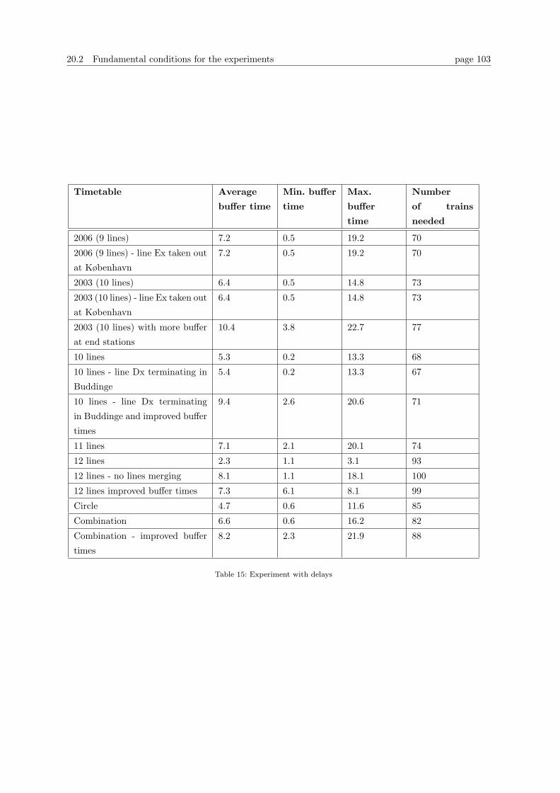
20.2 Fundamental conditions for the experiments page 103
Timetable Average
buffer time
Min. buffer
time
Max.
buffer
time
Number
of trains
needed
2006 (9 lines) 7.2 0.5 19.2 70
2006 (9 lines) - line Ex taken out
at København
7.2 0.5 19.2 70
2003 (10 lines) 6.4 0.5 14.8 73
2003 (10 lines) - line Ex taken out
at København
6.4 0.5 14.8 73
2003 (10 lines) with more buffer
at end stations
10.4 3.8 22.7 77
10 lines 5.3 0.2 13.3 68
10 lines - line Dx terminating in
Buddinge
5.4 0.2 13.3 67
10 lines - line Dx terminating
in Buddinge and improved buffer
times
9.4 2.6 20.6 71
11 lines 7.1 2.1 20.1 74
12 lines 2.3 1.1 3.1 93
12 lines - no lines merging 8.1 1.1 18.1 100
12 lines improved buffer times 7.3 6.1 8.1 99
Circle 4.7 0.6 11.6 85
Combination 6.6 0.6 16.2 82
Combination - improved buffer
times
8.2 2.3 21.9 88
Table 15: Experiment with delays
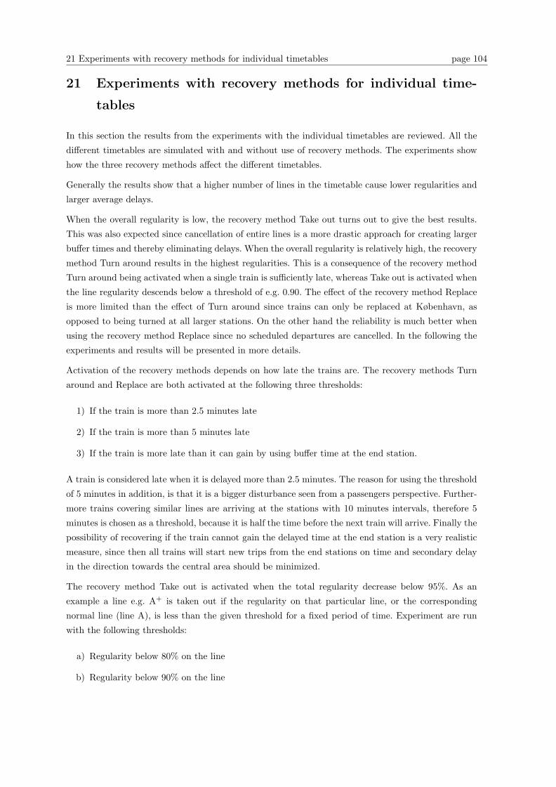
21 Experiments with recovery methods for individual timetables page 104
21 Experiments with recovery methods for individual time-
tables
In this section the results from the experiments with the individual timetables are reviewed. All the
different timetables are simulated with and without use of recovery methods. The experiments show
how the three recovery methods affect the different timetables.
Generally the results show that a higher number of lines in the timetable cause lower regularities and
larger average delays.
When the overall regularity is low, the recovery method Take out turns out to give the best results.
This was also expected since cancellation of entire lines is a more drastic approach for creating larger
buffer times and thereby eliminating delays. When the overall regularity is relatively high, the recovery
method Turn around results in the highest regularities. This is a consequence of the recovery method
Turn around being activated when a single train is sufficiently late, whereas Take out is activated when
the line regularity descends below a threshold of e.g. 0.90. The effect of the recovery method Replace
is more limited than the effect of Turn around since trains can only be replaced at København, as
opposed to being turned at all larger stations. On the other hand the reliability is much better when
using the recovery method Replace since no scheduled departures are cancelled. In the following the
experiments and results will be presented in more details.
Activation of the recovery methods depends on how late the trains are. The recovery methods Turn
around and Replace are both activated at the following three thresholds:
1) If the train is more than 2.5 minutes late
2) If the train is more than 5 minutes late
3) If the train is more late than it can gain by using buffer time at the end station.
A train is considered late when it is delayed more than 2.5 minutes. The reason for using the threshold
of 5 minutes in addition, is that it is a bigger disturbance seen from a passengers perspective. Further-
more trains covering similar lines are arriving at the stations with 10 minutes intervals, therefore 5
minutes is chosen as a threshold, because it is half the time before the next train will arrive. Finally the
possibility of recovering if the train cannot gain the delayed time at the end station is a very realistic
measure, since then all trains will start new trips from the end stations on time and secondary delay
in the direction towards the central area should be minimized.
The recovery method Take out is activated when the total regularity decrease below 95%. As an
example a line e.g. A+ is taken out if the regularity on that particular line, or the corresponding
normal line (line A), is less than the given threshold for a fixed period of time. Experiment are run
with the following thresholds:
a) Regularity below 80% on the line
b) Regularity below 90% on the line
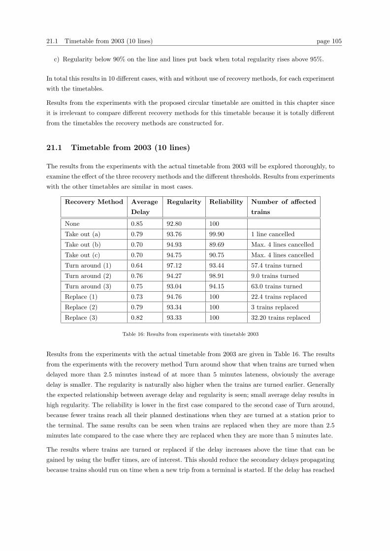
21.1 Timetable from 2003 (10 lines) page 105
c) Regularity below 90% on the line and lines put back when total regularity rises above 95%.
In total this results in 10 different cases, with and without use of recovery methods, for each experiment
with the timetables.
Results from the experiments with the proposed circular timetable are omitted in this chapter since
it is irrelevant to compare different recovery methods for this timetable because it is totally different
from the timetables the recovery methods are constructed for.
21.1 Timetable from 2003 (10 lines)
The results from the experiments with the actual timetable from 2003 will be explored thoroughly, to
examine the effect of the three recovery methods and the different thresholds. Results from experiments
with the other timetables are similar in most cases.
Recovery Method Average
Delay
Regularity Reliability Number of affected
trains
None 0.85 92.80 100
Take out (a) 0.79 93.76 99.90 1 line cancelled
Take out (b) 0.70 94.93 89.69 Max. 4 lines cancelled
Take out (c) 0.70 94.75 90.75 Max. 4 lines cancelled
Turn around (1) 0.64 97.12 93.44 57.4 trains turned
Turn around (2) 0.76 94.27 98.91 9.0 trains turned
Turn around (3) 0.75 93.04 94.15 63.0 trains turned
Replace (1) 0.73 94.76 100 22.4 trains replaced
Replace (2) 0.79 93.34 100 3 trains replaced
Replace (3) 0.82 93.33 100 32.20 trains replaced
Table 16: Results from experiments with timetable 2003
Results from the experiments with the actual timetable from 2003 are given in Table 16. The results
from the experiments with the recovery method Turn around show that when trains are turned when
delayed more than 2.5 minutes instead of at more than 5 minutes lateness, obviously the average
delay is smaller. The regularity is naturally also higher when the trains are turned earlier. Generally
the expected relationship between average delay and regularity is seen; small average delay results in
high regularity. The reliability is lower in the first case compared to the second case of Turn around,
because fewer trains reach all their planned destinations when they are turned at a station prior to
the terminal. The same results can be seen when trains are replaced when they are more than 2.5
minutes late compared to the case where they are replaced when they are more than 5 minutes late.
The results where trains are turned or replaced if the delay increases above the time that can be
gained by using the buffer times, are of interest. This should reduce the secondary delays propagating
because trains should run on time when a new trip from a terminal is started. If the delay has reached

21.2 Timetable for 2006 (9 lines) page 106
the limit where the train no longer is certain to run on time on the next trip, the recovery method is
activated. Depending on the average buffer time at the terminal station, meaning how much can be
gained at the end stations, this threshold gives better or worse results that by using 2.5 or 5 minutes
delay as threshold. Activating the recovery method when the train is more late than it can possibly
gain at the end station should be the most realistic solution, because there is no reason to use a
recovery method if the delay can be eliminated by using buffer times. In the real world a combination
of the three thresholds is probably used.
In the experiments with the recovery method Take out it is seen, that when the threshold for the
regularity on lines is set to 80% below which lines are taken out, the results for average delay and
regularity are worse than the situation where the threshold is set to 90%. This is not surprising since
trains with delays are kept longer in the system, in the first case, before they are taken out and
therefore affect the average delay and the regularity for a longer time. On the other hand keeping the
trains in the system longer has a positive effect on the reliability, and therefore the reliability is higher
in the first case.
Naturally it can be seen from the results that when the reliability decrease the regularity increase. Less
trains running will result in more buffer times between trains which decreases the risk of secondary
delays. Thereby the possibility of getting a better regularity increases.
Comparing the results for Take out (b) and Take out (c) it can be seen that the regularity is a little
bit higher and the reliability a little smaller when lines are not re-inserted (case b). The reason is that
when lines are re-inserted they increase the reliability on the line and the overall regularity decreases,
because there are more trains running in the system.
The recovery method Turn around gives the highest regularity in the experiments with the timetable
from 2003. The reason for this is that the regularity is reasonably high in the case where no recovery
method is applied. If the regularity was low in the case with no recovery, Take out would intuitively
turn out to be the best recovery method since this is a more drastic approach. The recovery method
Replace is not expected to be the best regarding regularity, since the recovery only takes place at one
station (København) as opposed to the other two recovery methods. When using Replace the reliability
is 100% no matter how many trains are replaced at København station. Naturally the passengers are
also disturbed when a train is replaced, but only the passengers in the train, not the passengers waiting
on the stations, since no departures are cancelled.
An additional experiment is made with the timetable from 2003. Instead of having line Ex running
continually between Køge and Østerport, the line starts in Køge, goes to Østerport and ends in
København where it is taken out. This is the actual structure of the plan for 2003. The experiment
results in a average regularity of 94.78%, which is a general improvement of 0.6 percentage points.
21.2 Timetable for 2006 (9 lines)
The results from the experiments with the actual timetable for 2006, shown in appendix J, are generally
very good and show that the plan is very robust. This is not surprising since only 9 lines are running,
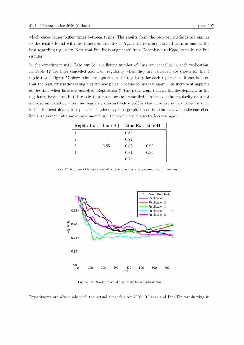
21.2 Timetable for 2006 (9 lines) page 107
which cause larger buffer times between trains. The results from the recovery methods are similar
to the results found with the timetable from 2003. Again the recovery method Turn around is the
best regarding regularity. Note that line Ex is augmented from København to Køge, to make the line
circular.
In the experiment with Take out (c) a different number of lines are cancelled in each replication.
In Table 17 the lines cancelled and their regularity when they are cancelled are shown for the 5
replications. Figure 57 shows the development in the regularity for each replication. It can be seen
that the regularity is decreasing and at some point it begins to increase again. The increment happens
at the time when lines are cancelled. Replication 3 (the green graph) shows the development in the
regularity best, since in this replication most lines are cancelled. The reason the regularity does not
increase immediately after the regularity descend below 95% is that lines are not cancelled at once
but at the next depot. In replication 1 (the navy blue graph) it can be seen that when the cancelled
line is re-inserted at time approximately 450 the regularity begins to decrease again.
Replication Line A+ Line Ex Line H+
1 0.82
2 0.87
3 0.95 0.86 0.90
4 0.87 0.90
5 0.75
Table 17: Number of lines cancelled and regularities in experiment with Take out (c)
0 100 200 300 400 500 600 7000.9
0.92
0.94
0.96
0.98
1
time
Reg
ular
ity
Mean RegularityReplication 1Replication 2Replication 3Replication 4Replication 5
Figure 57: Development of regularity for 5 replications
Experiments are also made with the actual timetable for 2006 (9 lines) and Line Ex terminating in

21.3 Proposed timetable with 10 lines page 108
København in the southern direction. Instead of having line Ex going in a circle between Køge and
Østerport, the line starts in Køge, goes to Østerport and ends in København where it is taken out.
It turns out that all results, with regards to regularity and average delays, are better when line Ex
is taken out at København. This is not surprising since there are less trains in the system that can
be disturbed and there is more buffer time between trains in the section from København to Køge
when line Ex does not run this distance. Surprisingly this small change has a very positive effect on
regularity. The regularity is improved with an average of 1.5 percentage points, which is a significant
improvement. This result indicates that line Ex has a low regularity and therefore a considerable
effect on the overall regularity. This indication is confirmed by examining the regularity on the lines
specifically. In the real plan developed for 2006 line Ex does not run from København to Køge.
21.3 Proposed timetable with 10 lines
Results from the experiments with the proposed timetable with 10 lines are given in Table 18.
Recovery Method Average
Delay
Regularity Reliability Number of affected
trains
None 1.37 85.49 100
Take out (a) 1.22 87.95 95.52 Max. 2 lines cancelled
Take out (b) 0.84 93.06 79.21 Max. 3 lines cancelled
Take out (c) 0.92 91.26 80.25 Max. 3 lines cancelled
Turn around (1) 0.70 96.72 94.34 56.8 trains turned
Turn around (2) 0.88 92.16 98.85 14 trains turned
Turn around (3) 0.69 95.29 84.23 111 trains turned
Replace (1) 0.83 93.80 100 43 trains replaced
Replace (2) 0.93 91.55 100 5 trains replaced
Replace (3) 0.89 92.19 100 59.4 trains replaced
Table 18: Results from experiments with proposed timetable with 10 lines
The interesting observation in these experiments is that the reliability in Turn around (1) is much
better than Turn around (3), even though the regularity is lower for Turn around (3). The low regularity
is a result of small buffer times in this timetable, which causes a large number of trains to be more
late than they can gain at the end stations, and thereby a large number of trains are being turned. A
higher regularity is reached in Turn around (1) even though fewer trains are turned. The reason for
this difference can be explained by the variation of trains being turned. When turning trains which
are delayed more than 2.5 minutes all trains in the network can be turned if delayed. On the contrary
when the threshold depends on the buffer time, which are different for the 10 lines, only some delays
can be eliminated.
As another experiment the proposed timetable with 10 lines has been modified such that line Dx
terminates in Buddinge. This has been done to make the proposed timetable more similar to the plan
from 2003, which also has 10 lines, including 3 lines to Høje Taastrup and only 2 lines to Farum, to

21.4 Combination timetable page 109
possibly get more comparable results. The results from the experiments with the modified version of
the timetable are shown in appendix J. The comparison of the timetable from 2003 and the proposed
timetable with 10 lines will be given in chapter 23.
When comparing the results from the two experiments with the proposed timetable with 10 lines (line
Dx terminating in Buddinge and Farum respectively), not surprisingly it turns out that shortening
line Dx results in a better regularity. In this case the regularity only improves with an average of 0.5
percentage point, which indicates that running line Dx all the way to Farum does not influence the
overall regularity much.
21.4 Combination timetable
Recovery Method Average
Delay
Regularity Reliability Number of affected
trains
None 0.80 93.35 100
Take out (a) 0.77 93.77 97.95 Max 1 line cancelled
Take out (b) 0.67 95.07 86.39 Max 3 line cancelled
Replace (1) 0.68 95.50 100 15 trains replaced
Replace (2) 0.70 94.90 100 3 trains replaced
Replace (3) 0.71 94.72 100 9 trains replaced
Table 19: Results from experiments with combination timetable
In the results from the experiments with the proposed combination timetable, given in Table 19, the
recovery method Replace gives the highest regularity. The regularity is considered high in the case
where no recovery method is being used, and therefore the regularity cannot be improved much by
cancelling lines, since this is done when the regularity gets below 95%. The recovery method Turn
around is not implemented since lines are relatively short, and therefore cannot be turned before the
end stations, hence it is not surprising that Replace gives the best results.
21.5 Timetable with 11 and 12 lines
The results from the experiments with the timetable with 11 lines, shown in Table 20, are generally
good, considering that the timetable has an extra line. The robustness is generally on the level of
the results from the experiments with the timetables with 10 lines. This indicates that not only the
number of lines affect the regularity. Further comparisons of the different timetables will be made later
in this chapter.
In the experiments with the timetable with 11 lines the recovery method Take out gives the highest
regularities. This is a result of a lower regularity when no recovery method is used, and therefore the
more drastic approach of cancelling entire lines should be the best method to obtain a high regularity.
The highest regularity also gives the lowest reliability because 4 lines must be cancelled to attain the

21.5 Timetable with 11 and 12 lines page 110
Recovery Method Average
Delay
Regularity Reliability Number of affected
trains
None 1.22 86.80 100
Take out (a) 0.82 93.67 87.30 Max 2 lines cancelled
Take out (b) 0.70 95.19 67.75 Max 4 lines cancelled
Turn around (1) 0.84 94.18 93.26 75 train turned
Turn around (2) 0.95 91.87 99.04 13 train turned
Turn around (3) 0.96 91.44 97.50 30 train turned
Replace (1) 1.02 90.47 100 26 train replaced
Replace (2) 1.09 88.91 100 9 train replaced
Replace (3) 1.08 89.32 100 23 train replaced
Table 20: Results from experiments with plan with 11 lines
high regularity.
Similarly in the experiments with the timetable with 12 lines the recovery method Take out also turns
out to be the best method, if concerned about a high regularity and low average delays. The results
can be seen in appendix J. Again Take out achieves the lowest reliability due to a large number of
scheduled departures being cancelled in order to obtain a high regularity. In the second case where
the lines are taken out if the total regularity decreases below 90%, all 6 lines possible (Ax, Axx, Bx,
Bxx, Cx and Cxx) are taken out and as a result the reliability is around 50% since half the number
of lines are taken out.

22 Other experiments page 111
22 Other experiments
In this chapter additional experiments with delays are conducted. It is shown that the regularity
is non-linearly decreasing when the probability of delay increases. Furthermore it is confirmed that
small and large delays have very different impacts on the regularity, and more interestingly that small
delays cause secondary delays when added to the large delays. In a third experiment with delays the
relationship between average delay and regularity is seen to be linear.
This chapter also examines experiments with buffer times. Results from several experiments show that
the amount of buffer time has a significant effect on the robustness of the timetable. More buffer time
results in less recovery needed to achieve higher regularities. Furthermore it is shown that the amount
of buffer time necessary to achieve a robust timetable is limited.
Last in this chapter it is confirmed that trains are waiting in queues for station and routes mainly in
the central area.
22.1 Experiments with delay
The delays added in the model are given by distributions and the probability of delay is determined to
fit a realistic regularity. Generally in the experiments the probability of delays occurring is set to 50.
Experiments are made to examine how the probability of delay affects the regularity. Four timetables
with respectively 9 lines (actual 2006), 10 lines (proposed timetable with improved buffer times), 11
and 12 lines are simulated with probability of delay set to 0, 10, 20, . . . , 100. All the experiments are
run without recovery methods.
0 100 200 300 400 500 600 700 800 900 10000.65
0.7
0.75
0.8
0.85
0.9
0.95
1
Time (minutes)
Reg
ular
ity
0% delay10% delay20% delay30% delay40% delay50% delay60% delay70% delay80% delay90% delay100% delay
Figure 58: Regularity for the different percentage delay
values
0 10 20 30 40 50 60 70 80 90 1000.2
0.3
0.4
0.5
0.6
0.7
0.8
0.9
1
Probability of delay
Reg
ular
ity
9 lines10 lines11 lines12 lines
Figure 59: Regularity as a function of probability of delay
for the four timetables
Figure 58 shows the regularity for the different probability values for the timetable with 9 lines. The
results confirm that a lower probability of delay results in a better regularity. The results also show
that this relationship is not linear. The change from probability e.g. 80% to 90% has a bigger negative
22.1 Experiments with delay page 112
effect on regularity than the change from 20% to 30% probability. Experiments with the other three
timetables give the same results only with other values on the y-axes. In Figure 59 the regularity after
750 minutes are shown as a function of probability of delay for all the timetables. Here it is seen that
the regularity is decreasing when the probability of delay is increasing. Note that the relationship is
not linear. This relationship can be explained because of secondary delay. Naturally the delays added
directly to the trains affect the regularity, but the secondary delays occurring because of the interaction
between the trains also affect the regularity.
22.1.1 Large and small delays
As explained earlier the delays added in the model are determined from historical data. The distri-
butions representing the delays are different for each station. For some stations the delays are bigger
than for others as it is in the real system. To examine how small and large delays affect the regularity
of the system, experiments with small and large delays are made separately. Because a definition of
small and large delays is difficult to determine, the median is used. The delays are divided into the
80 stations with the smallest delays and 81 stations with the largest delays. In the experiment with
smaller delays all the 81 distributions of larger delays are set to zero, meaning that no delays occur on
these 81 stations. Similarly for the experiment with large delays, the distributions for the small delays
are set to zero. This means that in both experiments delays are only occurring at half the stations as
opposed to the experiment with all delays, where delay might occur at all the stations. The experiment
with all the delays will therefore result in the lowest regularity.
Again the experiment is made with four timetables with respectively 9 lines (actual 2006), 10 lines
(proposed timetable with improved buffer times), 11 and 12 lines. The experiments are run with no
recovery and 100 % probability of delays. This means that at the stations where the delay distribution
is not zero, delay will be added every time a train enters the station.
The results of the experiments are shown in Figure 61 and 60. The figures show the regularity for
the timetables with respectively 11 and 12 lines. The results from the timetables with 9 and 10 lines
show the same results and can be seen in appendix J. Experiment with the same four timetables and a
percentage delay of 50% have also been conducted and results were similar. It is seen that even though
the definition of small and large delays is vague the results from the experiments with large and small
delays are very different. The regularity with only the large delay (the black curve) is an improvement
compared to the regularity for the simulation where all delay are added, but clearly the larger delays
have a negative effect on the regularity. The smaller delays have almost no effect on the regularity.
The simulation with only small delays (the blue curve) gives a very good regularity close to 100% (a
close-up shows that it is not exactly 100%). This can be explained by the possibility of gaining time
at each station by reducing dwell time to the minimum and by gaining time at the end stations. This
experiment also confirms that secondary delays have a big effect on regularity. Smaller delays alone
do not affect regularity, but omitting the smaller delays gives a considerably better regularity than
with all delays added. This is the effect of secondary delays.
This experiment confirms that large delays should be minimized and that a focus on larger delays is
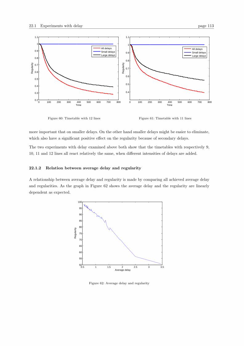
22.1 Experiments with delay page 113
0 100 200 300 400 500 600 700 8000.2
0.3
0.4
0.5
0.6
0.7
0.8
0.9
1
1.1
Time
Reg
ular
ity
All delaysSmall delaysLarge delays
Figure 60: Timetable with 12 lines
0 100 200 300 400 500 600 700 800
0.4
0.5
0.6
0.7
0.8
0.9
1
1.1
Time
Reg
ular
ity
All delaysSmall delaysLarge delays
Figure 61: Timetable with 11 lines
more important that on smaller delays. On the other hand smaller delays might be easier to eliminate,
which also have a significant positive effect on the regularity because of secondary delays.
The two experiments with delay examined above both show that the timetables with respectively 9,
10, 11 and 12 lines all react relatively the same, when different intensities of delays are added.
22.1.2 Relation between average delay and regularity
A relationship between average delay and regularity is made by comparing all achieved average delay
and regularities. As the graph in Figure 62 shows the average delay and the regularity are linearly
dependent as expected.
0.5 1 1.5 2 2.5 3 3.550
55
60
65
70
75
80
85
90
95
100
Average delay
Reg
ular
ity
Figure 62: Average delay and regularity
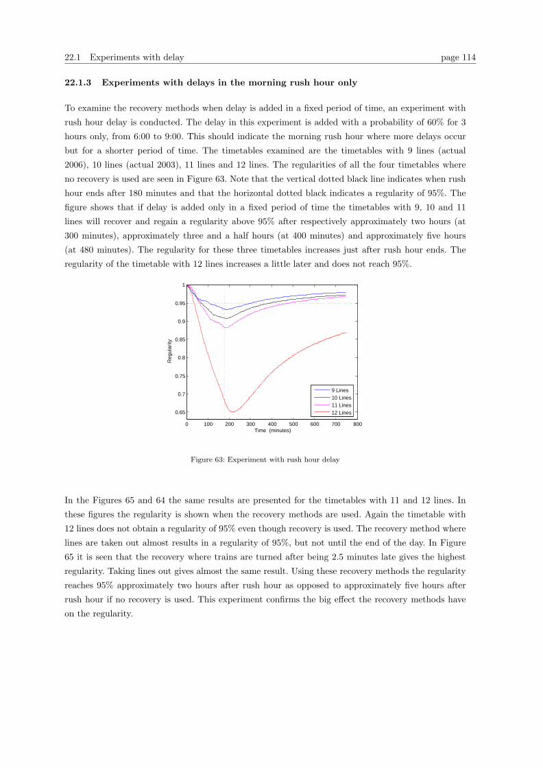
22.1 Experiments with delay page 114
22.1.3 Experiments with delays in the morning rush hour only
To examine the recovery methods when delay is added in a fixed period of time, an experiment with
rush hour delay is conducted. The delay in this experiment is added with a probability of 60% for 3
hours only, from 6:00 to 9:00. This should indicate the morning rush hour where more delays occur
but for a shorter period of time. The timetables examined are the timetables with 9 lines (actual
2006), 10 lines (actual 2003), 11 lines and 12 lines. The regularities of all the four timetables where
no recovery is used are seen in Figure 63. Note that the vertical dotted black line indicates when rush
hour ends after 180 minutes and that the horizontal dotted black indicates a regularity of 95%. The
figure shows that if delay is added only in a fixed period of time the timetables with 9, 10 and 11
lines will recover and regain a regularity above 95% after respectively approximately two hours (at
300 minutes), approximately three and a half hours (at 400 minutes) and approximately five hours
(at 480 minutes). The regularity for these three timetables increases just after rush hour ends. The
regularity of the timetable with 12 lines increases a little later and does not reach 95%.
0 100 200 300 400 500 600 700 800
0.65
0.7
0.75
0.8
0.85
0.9
0.95
1
Time (minutes)
Reg
ular
ity
9 Lines10 Lines11 Lines12 Lines
Figure 63: Experiment with rush hour delay
In the Figures 65 and 64 the same results are presented for the timetables with 11 and 12 lines. In
these figures the regularity is shown when the recovery methods are used. Again the timetable with
12 lines does not obtain a regularity of 95% even though recovery is used. The recovery method where
lines are taken out almost results in a regularity of 95%, but not until the end of the day. In Figure
65 it is seen that the recovery where trains are turned after being 2.5 minutes late gives the highest
regularity. Taking lines out gives almost the same result. Using these recovery methods the regularity
reaches 95% approximately two hours after rush hour as opposed to approximately five hours after
rush hour if no recovery is used. This experiment confirms the big effect the recovery methods have
on the regularity.
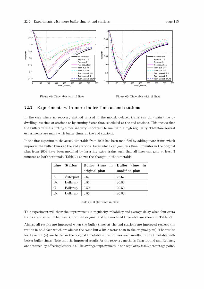
22.2 Experiments with more buffer time at end stations page 115
0 100 200 300 400 500 600 700 800
0.65
0.7
0.75
0.8
0.85
0.9
0.95
1
Time (minutes)
Reg
ular
ity
No recoveryReplace, 2.5Replace, 5Replace, shuntTake out, 0.8Take out, 0.9Turn around, 2.5Turn around, 5Turn around, shunt
Figure 64: Timetable with 12 lines
0 100 200 300 400 500 600 700 8000.88
0.9
0.92
0.94
0.96
0.98
1
Time (minutes)
Reg
ular
ity
No recoveryReplace, 2.5Replace, 5Replace, shuntTake out, 0.8Take out, 0.9Turn around, 2.5Turn around, 5Turn around, shunt
Figure 65: Timetable with 11 lines
22.2 Experiments with more buffer time at end stations
In the case where no recovery method is used in the model, delayed trains can only gain time by
dwelling less time at stations or by turning faster than scheduled at the end stations. This means that
the buffers in the shunting times are very important to maintain a high regularity. Therefore several
experiments are made with buffer times at the end stations.
In the first experiment the actual timetable from 2003 has been modified by adding more trains which
improves the buffer times at the end stations. Lines which can gain less than 3 minutes in the original
plan from 2003 have been modified by inserting extra trains such that all lines can gain at least 3
minutes at both terminals. Table 21 shows the changes in the timetable.
Line Station Buffer time in
original plan
Buffer time in
modified plan
A+ Østerport 2.67 22.67
Bx Hellerup 0.83 20.83
C Ballerup 0.50 20.50
Ex Hellerup 0.83 20.83
Table 21: Buffer times in plans
This experiment will show the improvement in regularity, reliability and average delay when four extra
trains are inserted. The results from the original and the modified timetable are shown in Table 22.
Almost all results are improved when the buffer times at the end stations are improved (except the
results in bold face which are almost the same but a little worse than in the original plan). The results
for Take out (a) are better in the original timetable since no lines are cancelled in the timetable with
better buffer times. Note that the improved results for the recovery methods Turn around and Replace,
are obtained by affecting less trains. The average improvement in the regularity is 0.3 percentage point.

22.2 Experiments with more buffer time at end stations page 116
Recovery Average Delay Regularity Reliability Trains affected
Original
2003
Modified
2003
Original
2003
Modified
2003
Original
2003
Modified
2003
Original
2003
Modified
2003
None 0.85 0.82 92.80 93.27 100 100 - -
Take out (a) 0.79 0.82 93.76 93.27 99.90 100 1 line 0
Take out (b) 0.70 0.74 94.93 94.48 89.69 88.65 4 lines 4 lines
Turn around (1) 0.64 0.60 97.12 97.84 93.44 95.10 57.4 45
Turn around (2) 0.76 0.72 94.27 94.71 98.91 99.29 9 7.8
Turn around (3) 0.75 0.75 93.04 94.21 94.15 99.56 63 4.2
Replace (1) 0.73 0.71 94.76 95.21 100 100 22.4 16
Replace (2) 0.79 0.75 93.34 94.15 100 100 3 1.6
Replace (3) 0.82 0.80 93.33 93.39 100 100 32.2 0.2
Table 22: Experiments with improved buffer times for the timetable from 2003
This might be considered a small improvement for the cost of four extra trains, but less recovery has to
be performed, which implies that the timetable becomes more robust when more buffer time is added.
The reliability is also improved when less recovery has to be performed to maintain the scheduled
plan. This implies an improvement in customer service level.
An experiment with the proposed timetable with 10 lines has also been conducted by modifying the
timetable such that all lines have buffer times larger than 2.5 minutes at the end stations. The modified
plan is made from the plan where line Dx terminates in Buddinge. Buffer times from the original plan
and for the modified plan can be seen in Table 23 for the lines where changes have occurred.
Line Station Original buffer time Modified buffer time
A and A+ Farum 0.6 20.6
E and E+ Hillerød 0.2 20.2
Table 23: Buffer times for experiment with improved buffer times in timetable with 10 lines
Generally the results for the modified version are better than the results from the original timetable.
The results can be seen in appendix J. An average of 5.4 trains are turned in the modified plan, which
is significantly lower than the average of 101.4 trains which are turned in the original timetable in
order to maintain the schedule. This implies that almost the same regularity can be obtained with
the modified timetable by turning approximately 20 times less trains than needed to obtain the same
regularity in the original plan.
The average regularity is improved by 2.9 percentage points, which is a significant improvement ob-
tained by using only 4 extra trains. Furthermore less recovery is needed to obtain a significantly better
result. The results show that even smaller improvements in the buffer times have a significant impact
on the overall regularity and average delay. Finally the experiment shows that not only is the regularity
improved but the timetable becomes more robust, since less recovery is needed.
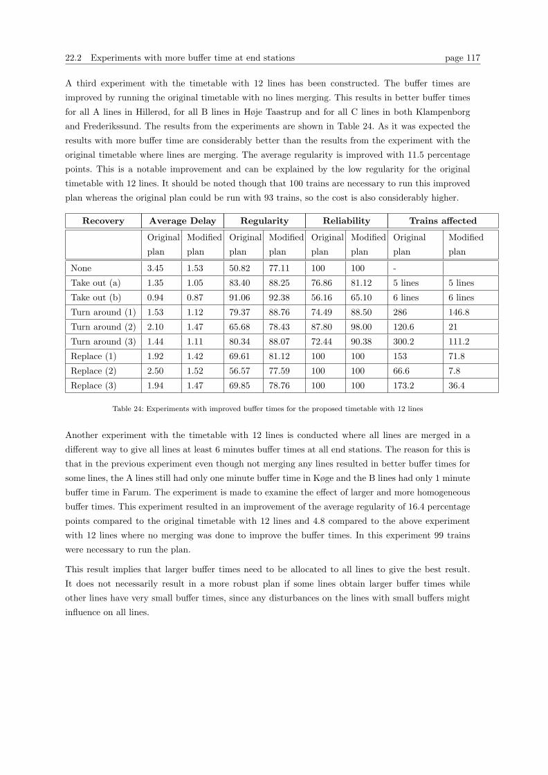
22.2 Experiments with more buffer time at end stations page 117
A third experiment with the timetable with 12 lines has been constructed. The buffer times are
improved by running the original timetable with no lines merging. This results in better buffer times
for all A lines in Hillerød, for all B lines in Høje Taastrup and for all C lines in both Klampenborg
and Frederikssund. The results from the experiments are shown in Table 24. As it was expected the
results with more buffer time are considerably better than the results from the experiment with the
original timetable where lines are merging. The average regularity is improved with 11.5 percentage
points. This is a notable improvement and can be explained by the low regularity for the original
timetable with 12 lines. It should be noted though that 100 trains are necessary to run this improved
plan whereas the original plan could be run with 93 trains, so the cost is also considerably higher.
Recovery Average Delay Regularity Reliability Trains affected
Original
plan
Modified
plan
Original
plan
Modified
plan
Original
plan
Modified
plan
Original
plan
Modified
plan
None 3.45 1.53 50.82 77.11 100 100 -
Take out (a) 1.35 1.05 83.40 88.25 76.86 81.12 5 lines 5 lines
Take out (b) 0.94 0.87 91.06 92.38 56.16 65.10 6 lines 6 lines
Turn around (1) 1.53 1.12 79.37 88.76 74.49 88.50 286 146.8
Turn around (2) 2.10 1.47 65.68 78.43 87.80 98.00 120.6 21
Turn around (3) 1.44 1.11 80.34 88.07 72.44 90.38 300.2 111.2
Replace (1) 1.92 1.42 69.61 81.12 100 100 153 71.8
Replace (2) 2.50 1.52 56.57 77.59 100 100 66.6 7.8
Replace (3) 1.94 1.47 69.85 78.76 100 100 173.2 36.4
Table 24: Experiments with improved buffer times for the proposed timetable with 12 lines
Another experiment with the timetable with 12 lines is conducted where all lines are merged in a
different way to give all lines at least 6 minutes buffer times at all end stations. The reason for this is
that in the previous experiment even though not merging any lines resulted in better buffer times for
some lines, the A lines still had only one minute buffer time in Køge and the B lines had only 1 minute
buffer time in Farum. The experiment is made to examine the effect of larger and more homogeneous
buffer times. This experiment resulted in an improvement of the average regularity of 16.4 percentage
points compared to the original timetable with 12 lines and 4.8 compared to the above experiment
with 12 lines where no merging was done to improve the buffer times. In this experiment 99 trains
were necessary to run the plan.
This result implies that larger buffer times need to be allocated to all lines to give the best result.
It does not necessarily result in a more robust plan if some lines obtain larger buffer times while
other lines have very small buffer times, since any disturbances on the lines with small buffers might
influence on all lines.
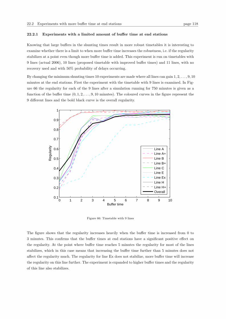
22.2 Experiments with more buffer time at end stations page 118
22.2.1 Experiments with a limited amount of buffer time at end stations
Knowing that large buffers in the shunting times result in more robust timetables it is interesting to
examine whether there is a limit to when more buffer time increases the robustness, i.e. if the regularity
stabilizes at a point even though more buffer time is added. This experiment is run on timetables with
9 lines (actual 2006), 10 lines (proposed timetable with improved buffer times) and 11 lines, with no
recovery used and with 50% probability of delays occurring.
By changing the minimum shunting times 10 experiments are made where all lines can gain 1, 2, . . . , 9, 10
minutes at the end stations. First the experiment with the timetable with 9 lines is examined. In Fig-
ure 66 the regularity for each of the 9 lines after a simulation running for 750 minutes is given as a
function of the buffer time (0, 1, 2, . . . , 9, 10 minutes). The coloured curves in the figure represent the
9 different lines and the bold black curve is the overall regularity.
0 1 2 3 4 5 6 7 8 9 100.1
0.2
0.3
0.4
0.5
0.6
0.7
0.8
0.9
1
Buffer time
Reg
ular
ity Line ALine A+Line BLine B+Line CLine ELine ExLine HLine H+Overall
Figure 66: Timetable with 9 lines
The figure shows that the regularity increases heavily when the buffer time is increased from 0 to
3 minutes. This confirms that the buffer times at end stations have a significant positive effect on
the regularity. At the point where buffer time reaches 5 minutes the regularity for most of the lines
stabilizes, which in this case means that increasing the buffer time further than 5 minutes does not
affect the regularity much. The regularity for line Ex does not stabilize, more buffer time will increase
the regularity on this line further. The experiment is expanded to higher buffer times and the regularity
of this line also stabilizes.

22.3 Homogeneous stopping pattern page 119
The experiments with timetables with 10 and 11 lines give similar results, see Figures 67 and 68. In the
experiment with the timetable with 10 lines the regularity also stabilize when the buffer time reaches
5 minutes, similar to the timetable with 9 lines, except that all the 10 lines reach stabilization and
many of the lines are already stabilized when buffer time reaches 3 minutes. In the experiment with
the timetable with 11 lines the regularity does not stabilize before the buffer time reaches 8 minutes.
Again a single line (line F) does not reach stabilization within the given buffer times.
0 1 2 3 4 5 6 7 8 9 100.1
0.2
0.3
0.4
0.5
0.6
0.7
0.8
0.9
1
Buffer time
Reg
ular
ity
Line ALine A+Line BLine B+Line CLine C+Line ELine E+Line FLine DxOverall
Figure 67: Timetable with 10 lines
0 1 2 3 4 5 6 7 8 9 100.1
0.2
0.3
0.4
0.5
0.6
0.7
0.8
0.9
1
Buffer time
Reg
ular
ity
Line ALine A+Line BLine B+Line CLine C+Line ELine E+Line FLine F+Line D+Overall
Figure 68: Timetable with 11 lines
Depending on the timetable and the line structure the limit for when more buffer time does not improve
the regularity any further will vary. This experiment shows that buffer time at end stations has a
positive effect on the regularity, but at some point the regularity will stabilize and more buffer time
will not improve the regularity further. Furthermore the experiment shows that for these timetables
the possibility of gaining minimum 3 to 5 minutes a the end station has a very positive effect on
regularity but more buffer times are not necessarily important, i.e. a few minutes of buffer time are
enough but very important.
22.3 Homogeneous stopping pattern
In the article Reliability and heterogeneity of railway services [23] it is concluded that the more homo-
geneous the timetable is according to stopping pattern, cycle time and line structure, the more robust
the plan will be.
Many of the timetables developed by DSB S-tog and used in this project use a combination of fast
and slow lines. Some lines cover all stations on train series and some lines skip smaller stations. There
are also big differences between cycle times for the different lines in the timetables. Some lines have a
cycle time of 200 and some only 120 minutes. This makes the timetables heterogeneous.
The proposed timetable with 10 lines is more homogeneous than the actual timetable from 2003 also
with 10 lines. It is more homogeneous according to cycle times and stopping patterns because all lines
in pairs stop at the same stations e.g. A and A+. When modified to be somewhat similar according to
22.4 Even distribution of tracks on København station page 120
buffer times at the end stations the more homogeneous timetable results in a higher regularity hence
a higher robustness.
The proposed timetable with 12 lines is considered to be very homogeneous concerning line structure
and stopping patterns. Only 3 different types of lines are used to cover the entire network. If other
similar timetables with 12 lines where accessible, the proposed timetable might have been proven to
be more robust than a less homogeneous timetable with 12 lines.
Because of the data available for this project, it has not been possible to fully confirm the hypotheses
about robustness and homogeneity. The timetables have to be compared on a very similar basis, which
is not possible, because a limited number of different timetables were accessible within the time frame
of this project.
22.4 Even distribution of tracks on København station
The hypothesis concerning even distribution of tracks on København station is explored. It is investi-
gated whether it can have a positive effect on regularity if trains are equally distributed between the
two tracks at København. Even headways should result in better buffer times between the trains for
all lines, and therefore it should improve the robustness of the plan. Note that there are two tracks in
each direction at København station.
In the proposed plan with 12 lines, the tracks are originally allocated such that all C line trains (C,
C+, Cx and Cxx) use the first track at København. All A line trains and all B line trains use the
second track. In this experiment every other line (given from their departure times at København)
use either the first or the second track at København respectively. A similar experiment is conducted
for the actual timetable from 2003.
The results did not show any improvements in neither regularity nor average delay. The reason is
probably that this minor improvement is too small to affect the results. In a scenario where tracks
were evenly distributed at all stations with double tracks an improvement might have been seen.
Therefore the hypothesis stating that even distribution of tracks will results in better regularity cannot
be accepted on the base of the results.
22.5 Numbers in queues
In the following the numbers of trains in queues for stations and queues for routes are explored. In
Table 25 the numbers in queues for the stations are observed for all the main timetables, run with
delays but without recovery. It is assumed that the numbers will be similarly distributed for the
different timetables if recovery was used (naturally the average number in queue would be smaller).
In Table 26 the numbers of trains in queue for the routes to the stations are shown. In the tables
the maximum number in queue for the 5 replications are observed. Only stations and routes where a
maximum number of 2 or more trains in queue appeared are included. It can be seen that most of the
stations and routes where queues occur, are in the central section, which was also the expected result,
22.5 Numbers in queues page 121
because all the trains are travelling through this section of the network. Furthermore Enghave station
appears to have a maximum of 2 trains in queue for a large number of the timetables. This is probably
because several lines meet in Valby before going to Enghave and then to Dybbølsbro, and both Valby
in the northern direction and Dybbølsbro have double tracks, and therefore Enghave, which has a
single track only, defines a bottleneck. This results in queues.
Note that there are no trains in queues for the stations when simulating the timetable for 2006. Note
also that the results for the circular timetable have been omitted, due to the different structure.
It should be noted from comparing the two tables that the number of queues for the routes is somewhat
larger than the number of queues for the stations. This is due to the way safe headways are handled
in the model. Trains are held back on the routes to maintain safe headways in the model. Queue on a
station occurs when the station is occupied by another train. This situation only arises when a trains
is delayed more than 90 seconds at the station, because otherwise the next train will be held back
at the route to the station. For example if a train is delayed 30 seconds at Enghave this does not
influence the next train because it arrives at least 90 seconds later due to the safe headways on the
routes. Naturally these numbers does not apply for the larger stations where the dwell time alone is
30-60 seconds and therefore a smaller amount of delay will cause a queue on the station. This might
also be the reason for the largest queues arising in the central section, because this is where the dwell
times are largest (30 seconds on most stations) and also the largest amounts of delays occur, because
of the large number of passengers etc. Therefore the risks of queues at the stations in the central
section are larger, not only because all trains are travelling through these section.
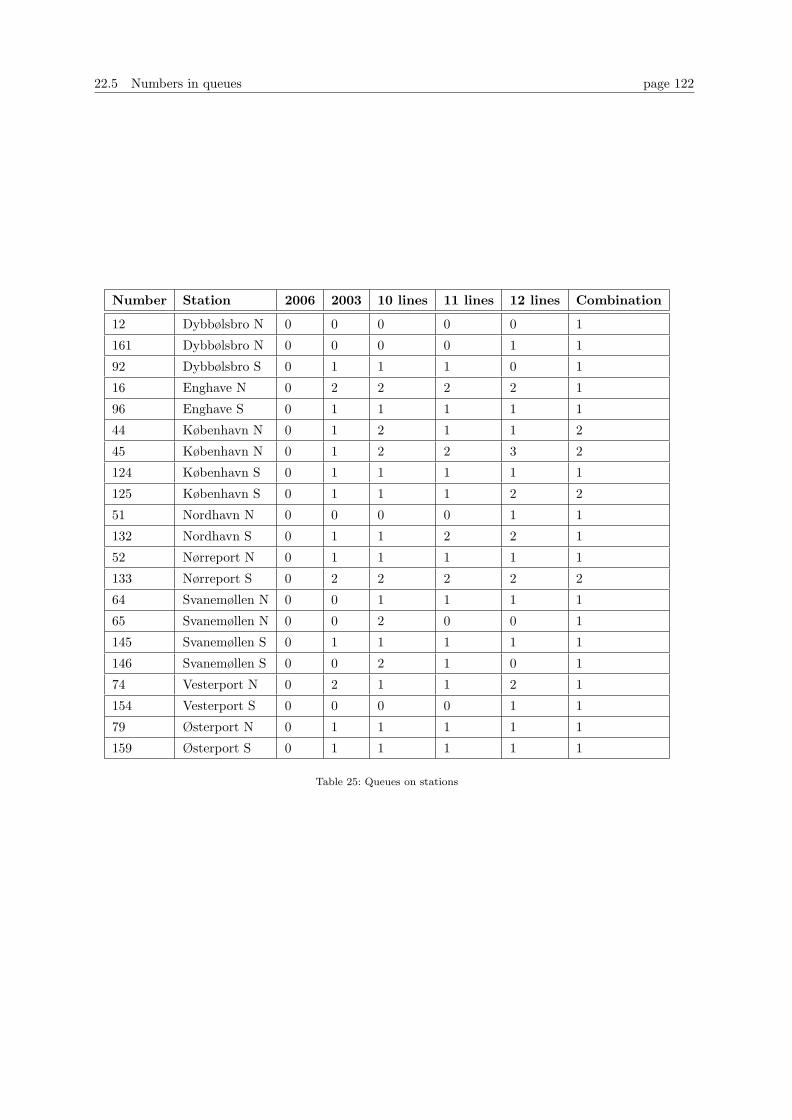
22.5 Numbers in queues page 122
Number Station 2006 2003 10 lines 11 lines 12 lines Combination
12 Dybbølsbro N 0 0 0 0 0 1
161 Dybbølsbro N 0 0 0 0 1 1
92 Dybbølsbro S 0 1 1 1 0 1
16 Enghave N 0 2 2 2 2 1
96 Enghave S 0 1 1 1 1 1
44 København N 0 1 2 1 1 2
45 København N 0 1 2 2 3 2
124 København S 0 1 1 1 1 1
125 København S 0 1 1 1 2 2
51 Nordhavn N 0 0 0 0 1 1
132 Nordhavn S 0 1 1 2 2 1
52 Nørreport N 0 1 1 1 1 1
133 Nørreport S 0 2 2 2 2 2
64 Svanemøllen N 0 0 1 1 1 1
65 Svanemøllen N 0 0 2 0 0 1
145 Svanemøllen S 0 1 1 1 1 1
146 Svanemøllen S 0 0 2 1 0 1
74 Vesterport N 0 2 1 1 2 1
154 Vesterport S 0 0 0 0 1 1
79 Østerport N 0 1 1 1 1 1
159 Østerport S 0 1 1 1 1 1
Table 25: Queues on stations
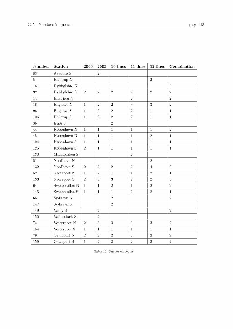
22.5 Numbers in queues page 123
Number Station 2006 2003 10 lines 11 lines 12 lines Combination
83 Avedøre S 2
5 Ballerup N 2
161 Dybbølsbro N 2
92 Dybbølsbro S 2 2 2 2 2 2
14 Ellebjerg N 2 2
16 Enghave N 1 2 2 3 3 2
96 Enghave S 1 2 2 2 1 1
106 Hellerup S 1 2 2 2 1 1
36 Ishøj S 2
44 København N 1 1 1 1 1 2
45 København N 1 1 1 1 2 1
124 København S 1 1 1 1 1 1
125 København S 2 1 1 1 1 1
130 Malmparken S 2
51 Nordhavn N 2
132 Nordhavn S 2 2 2 2 4 2
52 Nørreport N 1 2 1 1 2 1
133 Nørreport S 2 3 3 2 2 3
64 Svanemøllen N 1 1 2 1 2 2
145 Svanemøllen S 1 1 1 2 2 1
66 Sydhavn N 2 2
147 Sydhavn S 2
149 Valby S 2 2
150 Vallensbæk S 2
74 Vesterport N 2 3 3 3 3 2
154 Vesterport S 1 1 1 1 1 1
79 Østerport N 2 2 2 2 2 2
159 Østerport S 1 2 2 2 2 2
Table 26: Queues on routes
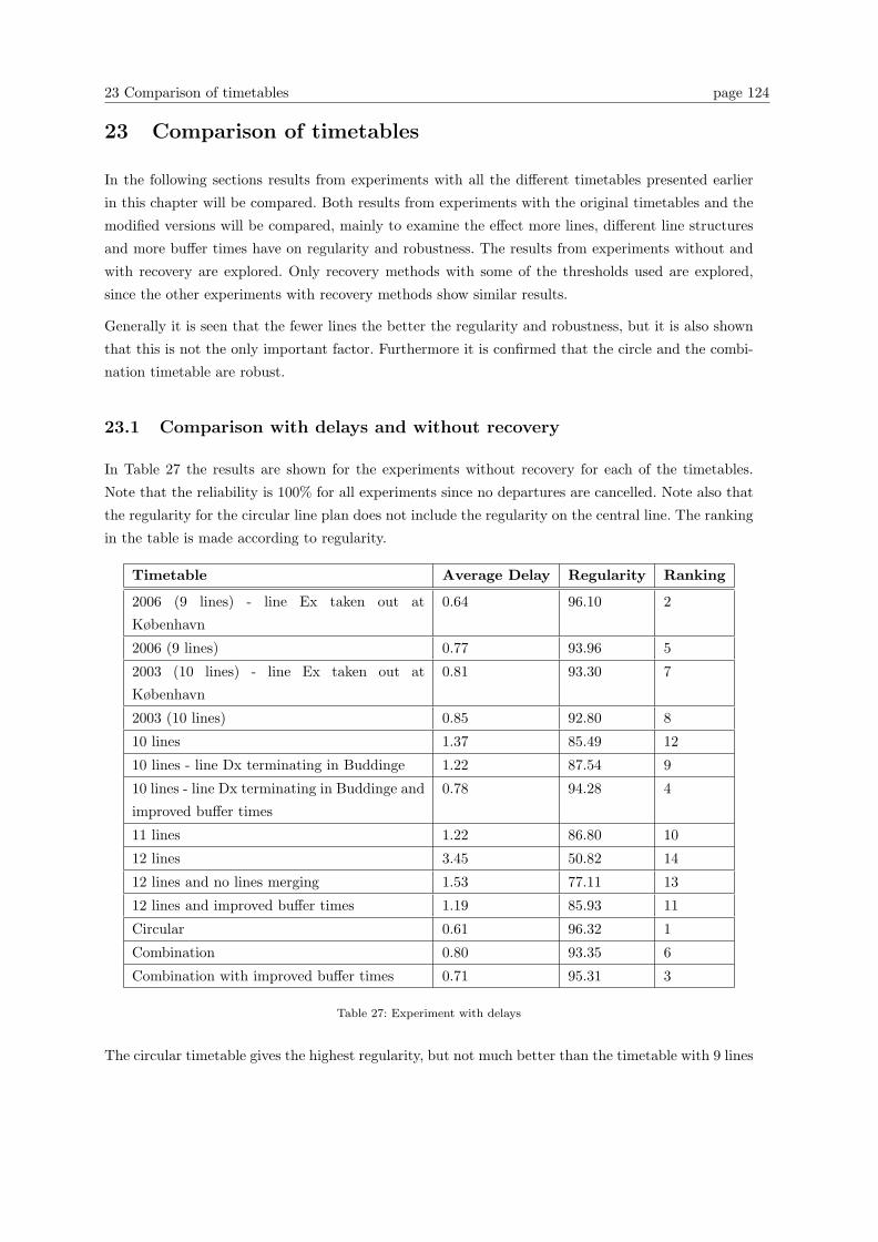
23 Comparison of timetables page 124
23 Comparison of timetables
In the following sections results from experiments with all the different timetables presented earlier
in this chapter will be compared. Both results from experiments with the original timetables and the
modified versions will be compared, mainly to examine the effect more lines, different line structures
and more buffer times have on regularity and robustness. The results from experiments without and
with recovery are explored. Only recovery methods with some of the thresholds used are explored,
since the other experiments with recovery methods show similar results.
Generally it is seen that the fewer lines the better the regularity and robustness, but it is also shown
that this is not the only important factor. Furthermore it is confirmed that the circle and the combi-
nation timetable are robust.
23.1 Comparison with delays and without recovery
In Table 27 the results are shown for the experiments without recovery for each of the timetables.
Note that the reliability is 100% for all experiments since no departures are cancelled. Note also that
the regularity for the circular line plan does not include the regularity on the central line. The ranking
in the table is made according to regularity.
Timetable Average Delay Regularity Ranking
2006 (9 lines) - line Ex taken out at
København
0.64 96.10 2
2006 (9 lines) 0.77 93.96 5
2003 (10 lines) - line Ex taken out at
København
0.81 93.30 7
2003 (10 lines) 0.85 92.80 8
10 lines 1.37 85.49 12
10 lines - line Dx terminating in Buddinge 1.22 87.54 9
10 lines - line Dx terminating in Buddinge and
improved buffer times
0.78 94.28 4
11 lines 1.22 86.80 10
12 lines 3.45 50.82 14
12 lines and no lines merging 1.53 77.11 13
12 lines and improved buffer times 1.19 85.93 11
Circular 0.61 96.32 1
Combination 0.80 93.35 6
Combination with improved buffer times 0.71 95.31 3
Table 27: Experiment with delays
The circular timetable gives the highest regularity, but not much better than the timetable with 9 lines
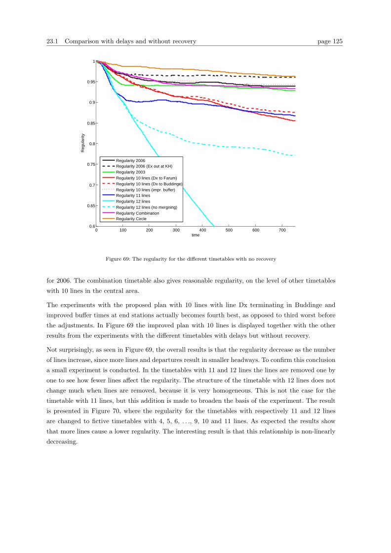
23.1 Comparison with delays and without recovery page 125
0 100 200 300 400 500 600 7000.6
0.65
0.7
0.75
0.8
0.85
0.9
0.95
1
time
Reg
ular
ity
Regularity 2006Regularity 2006 (Ex out at KH)Regularity 2003Regularity 10 lines (Dx to Farum)Regularity 10 lines (Dx to Buddinge)Regularity 10 lines (impr. buffer)Regularity 11 linesRegularity 12 linesRegularity 12 lines (no mergning)Regularity CombinationRegularity Circle
Figure 69: The regularity for the different timetables with no recovery
for 2006. The combination timetable also gives reasonable regularity, on the level of other timetables
with 10 lines in the central area.
The experiments with the proposed plan with 10 lines with line Dx terminating in Buddinge and
improved buffer times at end stations actually becomes fourth best, as opposed to third worst before
the adjustments. In Figure 69 the improved plan with 10 lines is displayed together with the other
results from the experiments with the different timetables with delays but without recovery.
Not surprisingly, as seen in Figure 69, the overall results is that the regularity decrease as the number
of lines increase, since more lines and departures result in smaller headways. To confirm this conclusion
a small experiment is conducted. In the timetables with 11 and 12 lines the lines are removed one by
one to see how fewer lines affect the regularity. The structure of the timetable with 12 lines does not
change much when lines are removed, because it is very homogeneous. This is not the case for the
timetable with 11 lines, but this addition is made to broaden the basis of the experiment. The result
is presented in Figure 70, where the regularity for the timetables with respectively 11 and 12 lines
are changed to fictive timetables with 4, 5, 6, . . ., 9, 10 and 11 lines. As expected the results show
that more lines cause a lower regularity. The interesting result is that this relationship is non-linearly
decreasing.
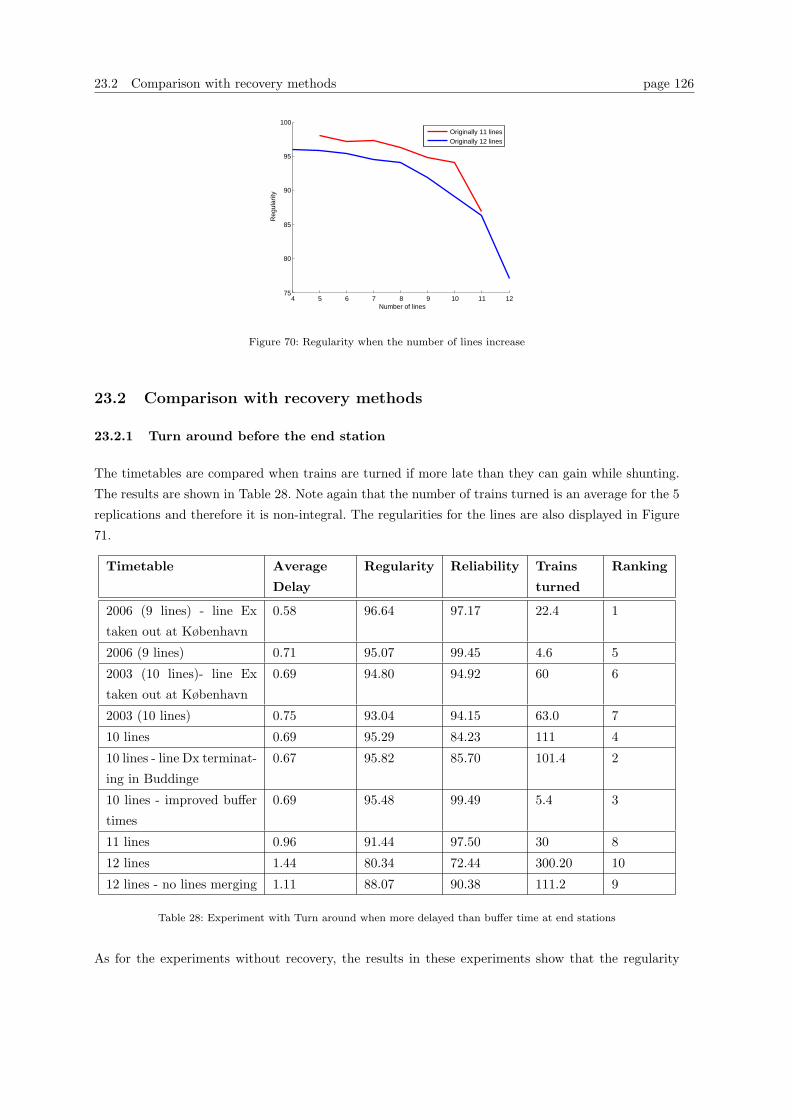
23.2 Comparison with recovery methods page 126
4 5 6 7 8 9 10 11 1275
80
85
90
95
100
Number of lines
Reg
ular
ity
Originally 11 linesOriginally 12 lines
Figure 70: Regularity when the number of lines increase
23.2 Comparison with recovery methods
23.2.1 Turn around before the end station
The timetables are compared when trains are turned if more late than they can gain while shunting.
The results are shown in Table 28. Note again that the number of trains turned is an average for the 5
replications and therefore it is non-integral. The regularities for the lines are also displayed in Figure
71.
Timetable Average
Delay
Regularity Reliability Trains
turned
Ranking
2006 (9 lines) - line Ex
taken out at København
0.58 96.64 97.17 22.4 1
2006 (9 lines) 0.71 95.07 99.45 4.6 5
2003 (10 lines)- line Ex
taken out at København
0.69 94.80 94.92 60 6
2003 (10 lines) 0.75 93.04 94.15 63.0 7
10 lines 0.69 95.29 84.23 111 4
10 lines - line Dx terminat-
ing in Buddinge
0.67 95.82 85.70 101.4 2
10 lines - improved buffer
times
0.69 95.48 99.49 5.4 3
11 lines 0.96 91.44 97.50 30 8
12 lines 1.44 80.34 72.44 300.20 10
12 lines - no lines merging 1.11 88.07 90.38 111.2 9
Table 28: Experiment with Turn around when more delayed than buffer time at end stations
As for the experiments without recovery, the results in these experiments show that the regularity
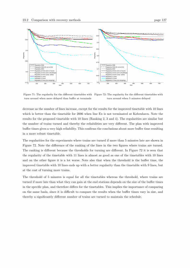
23.2 Comparison with recovery methods page 127
0 100 200 300 400 500 600 7000.75
0.8
0.85
0.9
0.95
1
time
Reg
ular
ity
Regularity 2006Regularity 2006 (Ex out at KH)Regularity 2003Regularity 10 lines (Dx to Farum)Regularity 10 lines (Dx to Buddinge)Regularity 10 lines (impr. buffer)Regularity 11 linesRegularity 12 linesRegularity 12 lines (no mergning)
Figure 71: The regularity for the different timetables with
turn around when more delayed than buffer at terminals
0 100 200 300 400 500 600 7000.6
0.65
0.7
0.75
0.8
0.85
0.9
0.95
1
time
Reg
ular
ity
Regularity 2006Regularity 2006 (Ex out at KH)Regularity 2003Regularity 10 lines (Dx to Farum)Regularity 10 lines (Dx to Buddinge)Regularity 10 lines (impr. buffer)Regularity 11 linesRegularity 12 linesRegularity 12 lines (no mergning)
Figure 72: The regularity for the different timetables with
turn around when 5 minutes delayed
decrease as the number of lines increase, except for the results for the improved timetable with 10 lines
which is better than the timetable for 2006 when line Ex is not terminated at København. Note the
results for the proposed timetable with 10 lines (Ranking 2, 3 and 4). The regularities are similar but
the number of trains turned and thereby the reliabilities are very different. The plan with improved
buffer times gives a very high reliability. This confirms the conclusions about more buffer time resulting
in a more robust timetable.
The regularities for the experiments where trains are turned if more than 5 minutes late are shown in
Figure 72. Note the difference of the ranking of the lines in the two figures where trains are turned.
The ranking is different because the thresholds for turning are different. In Figure 72 it is seen that
the regularity of the timetable with 11 lines is almost as good as one of the timetables with 10 lines
and on the other figure it is a lot worse. Note also that when the threshold is the buffer time, the
improved timetable with 10 lines ends up with a better regularity than the timetable with 9 lines, but
at the cost of turning more trains.
The threshold of 5 minutes is equal for all the timetables whereas the threshold, where trains are
turned if more late than what they can gain at the end stations depends on the size of the buffer times
in the specific plan, and therefore differs for the timetables. This implies the importance of comparing
on the same basis, since it is difficult to compare the results when the buffer times vary in size, and
thereby a significantly different number of trains are turned to maintain the schedule.
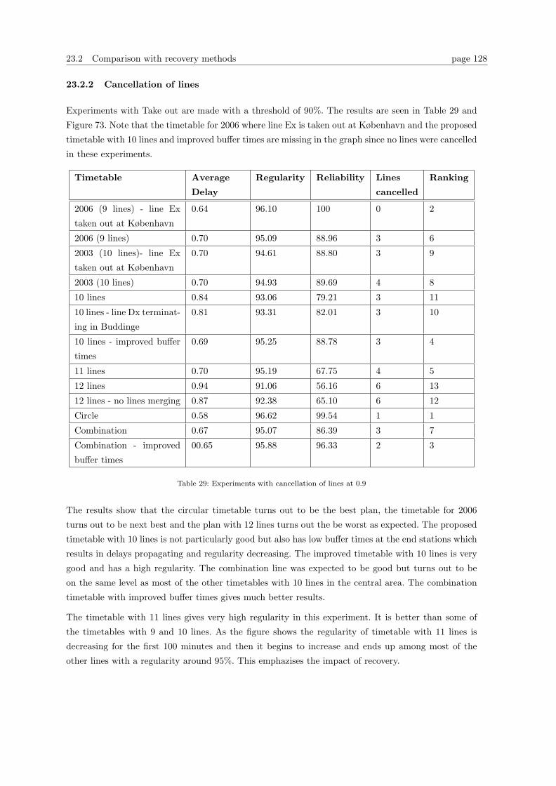
23.2 Comparison with recovery methods page 128
23.2.2 Cancellation of lines
Experiments with Take out are made with a threshold of 90%. The results are seen in Table 29 and
Figure 73. Note that the timetable for 2006 where line Ex is taken out at København and the proposed
timetable with 10 lines and improved buffer times are missing in the graph since no lines were cancelled
in these experiments.
Timetable Average
Delay
Regularity Reliability Lines
cancelled
Ranking
2006 (9 lines) - line Ex
taken out at København
0.64 96.10 100 0 2
2006 (9 lines) 0.70 95.09 88.96 3 6
2003 (10 lines)- line Ex
taken out at København
0.70 94.61 88.80 3 9
2003 (10 lines) 0.70 94.93 89.69 4 8
10 lines 0.84 93.06 79.21 3 11
10 lines - line Dx terminat-
ing in Buddinge
0.81 93.31 82.01 3 10
10 lines - improved buffer
times
0.69 95.25 88.78 3 4
11 lines 0.70 95.19 67.75 4 5
12 lines 0.94 91.06 56.16 6 13
12 lines - no lines merging 0.87 92.38 65.10 6 12
Circle 0.58 96.62 99.54 1 1
Combination 0.67 95.07 86.39 3 7
Combination - improved
buffer times
00.65 95.88 96.33 2 3
Table 29: Experiments with cancellation of lines at 0.9
The results show that the circular timetable turns out to be the best plan, the timetable for 2006
turns out to be next best and the plan with 12 lines turns out the be worst as expected. The proposed
timetable with 10 lines is not particularly good but also has low buffer times at the end stations which
results in delays propagating and regularity decreasing. The improved timetable with 10 lines is very
good and has a high regularity. The combination line was expected to be good but turns out to be
on the same level as most of the other timetables with 10 lines in the central area. The combination
timetable with improved buffer times gives much better results.
The timetable with 11 lines gives very high regularity in this experiment. It is better than some of
the timetables with 9 and 10 lines. As the figure shows the regularity of timetable with 11 lines is
decreasing for the first 100 minutes and then it begins to increase and ends up among most of the
other lines with a regularity around 95%. This emphazises the impact of recovery.
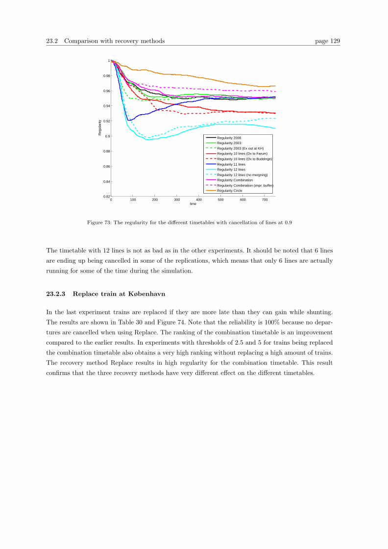
23.2 Comparison with recovery methods page 129
0 100 200 300 400 500 600 7000.82
0.84
0.86
0.88
0.9
0.92
0.94
0.96
0.98
1
time
Reg
ular
ity
Regularity 2006
Regularity 2003
Regularity 2003 (Ex out at KH)
Regularity 10 lines (Dx to Farum)
Regularity 10 lines (Dx to Buddinge)
Regularity 11 lines
Regularity 12 lines
Regularity 12 lines (no mergning)
Regularity Combination
Regularity Combination (impr. buffer)
Regularity Circle
Figure 73: The regularity for the different timetables with cancellation of lines at 0.9
The timetable with 12 lines is not as bad as in the other experiments. It should be noted that 6 lines
are ending up being cancelled in some of the replications, which means that only 6 lines are actually
running for some of the time during the simulation.
23.2.3 Replace train at København
In the last experiment trains are replaced if they are more late than they can gain while shunting.
The results are shown in Table 30 and Figure 74. Note that the reliability is 100% because no depar-
tures are cancelled when using Replace. The ranking of the combination timetable is an improvement
compared to the earlier results. In experiments with thresholds of 2.5 and 5 for trains being replaced
the combination timetable also obtains a very high ranking without replacing a high amount of trains.
The recovery method Replace results in high regularity for the combination timetable. This result
confirms that the three recovery methods have very different effect on the different timetables.

23.2 Comparison with recovery methods page 130
Timetable Average
Delay
Regularity Reliability Trains
replaced
Ranking
2006 (9 lines) - line Ex
taken out at København
0.63 96.15 100 12.8 1
2006 (9 lines) 0.75 94.35 100 11.4 6
2003 (10 lines) - line Ex
taken out at København
0.75 94.65 100 23.6 5
2003 (10 lines) 0.82 93.33 100 32.20 7
10 lines 0.89 92.19 100 59.4 9
10 lines - line Dx terminat-
ing in Buddinge
0.88 92.22 100 56 8
10 lines - improved buffer
times
0.74 94.85 100 0.6 3
11 lines 1.08 89.32 100 23 10
12 lines 1.94 69.85 100 173.2 12
12 lines - no lines merging 1.47 78.76 100 36.4 11
Combination 0.71 94.72 100 9 4
Combination - improved
buffer times
0.68 95.53 100 0.6 2
Table 30: Experiment with Replace when more delayed than buffer time at terminals
0 100 200 300 400 500 600 7000.6
0.65
0.7
0.75
0.8
0.85
0.9
0.95
1
time
Reg
ular
ity
Regularity 2006
Regularity 2006 (Ex out at KH)
Regularity 2003
Regularity 10 lines (Dx to Farum)
Regularity 10 lines (Dx to Buddinge)
Regularity 10 lines (impr. buffer)
Regularity 11 lines
Regularity 12 lines
Regularity 12 lines (no mergning)
Regularity Combination
Figure 74: The regularity for the different timetables with Replace when more delayed than slack time at end stations

24 Conclusion on the experiments page 131
24 Conclusion on the experiments
The conclusion on the experiments with the three recovery methods is that when the overall regularity
is high, turning trains gives the best overall results with regards to both regularity, average delay and
reliability. Cancelling lines is only activated when the regularity is low and therefore this recovery
method is appropriate for medium and larger disturbances. The recovery method of cancelling lines
generally has the worst reliability. Replacing trains is not as effective as turning trains, because the
trains can be replaced at København station only. On the other hand this recovery method has a very
high reliability, since no departures are cancelled, which means that only the passengers in the train
that is scheduled to be replaced are affected.
The experiments with delay showed that more delay results in lower regularity, and the relation is non-
linearly decreasing. Another conclusion is that large delays naturally have a more significant effect on
regularity than smaller delays, but also that secondary delays have a significant impact on regularity,
so smaller delays should also be eliminated if possible.
One of the main conclusions from the experiments is that the amount of buffer time at the end stations
has a considerable effect on the robustness. A minimum of three to five minutes (in these experiments)
of buffer at the end stations results in high regularity and few trains affected when the recovery
methods are used. This indicates that a timetable becomes more robust when a reasonable amount
of buffer time is used. Furthermore it is shown that the necessary amount of buffer time is limited,
which makes it realistic to implement the result. It should be noted though, that if more buffer time
is added more trains are needed, which is a negative result seen from an economical point of view.
Since the amount of necessary buffer time is limited it should be possible to construct timetables with
reasonable buffer times to achieve a higher robustness.
Investigating the occurrences and sizes of queues showed that most of the stations and routes where
queues occur, are in the central section, which was also the expected result, because all the trains are
travelling through this section of the network. Furthermore it was concluded that an additional reason
for the queues arising in the central section was because of the larger dwell times and higher amounts
of delays.
The conclusion for the comparison of the different timetables is that not surprisingly the number of
lines in a timetable seems to have a significant impact on the regularity and thereby robustness of the
plan. In general a higher number of lines, with the same frequency of 20 minutes on all lines, results
in a lower regularity. Overall the improved timetable with 10 lines turns out to give the best results
with regards to number of lines, regularity and number of affected trains. The timetable for 2006 is
also very good, but the consequence of this plan is a lower customer service level since it includes one
line less. Furthermore it is concluded that the number of lines is not the only important factor when
considering robustness of a timetable. A timetable with 10 lines is shown to have a higher regularity
than a timetable with 9 lines because of better buffer times at the end stations.
A larger number of lines and the same frequencies results in a larger number of departures, which
improves the customer service level. Therefore it would be desirable if it was possible to use a timetable
24 Conclusion on the experiments page 132
with more than 10 lines, to raise the customer service level. The conclusion from the experiments with
the timetable with 12 lines is that the achieved regularities are not acceptable. A regularity of 88.76%
is obtained with the timetable with 12 lines and no lines merging when trains are turned. The highest
regularity of 92.38% is achieved when lines are cancelled. This is a reasonable regularity, but the
result should not be accounted for in recommending running 12 lines since the higher regularity was
achieved by cancelling 5-6 lines. The timetable with 11 lines might be possible though since some of
the experiments resulted in a regularity at the same level as for the timetables with 10 lines.
The constructed circular timetable resulted in high regularity as expected. It is better than all the
other timetables in all the experiments. It should be noted though, that the timetable with 9 lines is
almost as good. The regularity is only approximately 0.4 percentage points lower for the timetable for
2006. The combination timetable can be compared with the other timetables with 10 lines through the
central area. It is better that these timetables in all the experiments where the combination timetable
has improved buffer times. This is not surprising, because the lines are shorter in the combination
timetable. Note that the circular and combination timetables are not necessarily directly compatible
with the current structure of S-train network. These two timetables are meant as prototypes and have
the purpose of testing an entirely new line structure.
25 Further research page 133
25 Further research
In this chapter it is discussed how the model can be expanded to broaden the use of it or to increase
the level of detail. Furthermore some additional experiments are mentioned.
25.1 Further development of the model
To make the recovery strategies more realistic additional recovery methods could be implemented, but
most importantly the recovery methods should be combined in a way in accordance with how recovery
is done in the real system. A decision tool for which recovery method to use in particular situations
should be developed to make the recovery methods more realistic. This involves analyzing in detail,
when different recovery methods are applied by the controllers.
The delay added in the model is made from historical data, which makes it very trustworthy. In the
historical data both late and early trains are observed. Since an assumption about trains never leaving
earlier than scheduled is made, the delay distributions are not directly applicable in the model. In the
model compensation is made by only adding delay every second time a train enters a station (delay
is added with 50% probability). To make the results more accurate two things can be done. Either
the assumption should be adjusted and letting trains depart earlier at stations. This way the delay
distribution would be strictly correct. Another way to make the model more accurate could be to
determine a more precise delay probability instead of 50%.
Furthermore some other assumptions made in the model could be adjusted to increase the degree of
detail in the model. Generally the assumptions concerning only examining a worst case scenario could
be omitted to broaden the use of the model. This means that data should be modified to simulate a
day in details and not only rush hour situations, with regards to number of trains used, lines inserted
and cancelled etc. Concerns about marshalling and train specific data could also be added to broaden
the use of the model.
Overtaking could be made possible. In Arena this can be done by using a Resource module for the
platforms instead of a Hold and a Delay module. At a station where overtaking is possible there are
two tracks. A Resource with capacity 2, could be used to represent the two tracks. This would imply
the need for a ranking rule, to specify the order of the entities in the queue to the resource (the
station). This way a train with a higher rank could enter the station earlier than one with a lower
rank, if they are both waiting to enter the station. Furthermore it might be possible to gain time at
a few routes in case of delays. This could also be implemented in the model if possible.
To increase the level of detail in the model the correct headways in the entire network could be added.
This is very simple to implement, but the information have not been available for this project.
In the real system there is only one track between Farum and Værløse because of an old bridge
(Fiskebækbro). The trains use the same track in both directions. This is omitted in the model, but
could be implemented by adding a fictive station between Farum and Værløse which trains in both
directions should visit.
25.2 Further experiments page 134
Finally it would be an improvement in the model if additional measures of the number of primary and
secondary delays were included, to make it easier to display where the problems occur in the network.
This is a difficult task, and requires very specific definitions on how primary delays are measured.
25.2 Further experiments
- The comparison of the timetables could be expanded with more timetables to generalize the
results. Furthermore timetables which were identical except for one feature could be of use to
determine more thoroughly whether a specific hypothesis could be accepted.
- Experiments where the trains may switch to another platform if the scheduled platform is oc-
cupied should minimize secondary delays. The result is investigated in [4] and could be demon-
strated using the model developed in this project. In Arena switching between platforms can be
implemented by using resources for the platforms.
- Experiments with double tracks at all the stations in the central area (Dybbølsbro to Svanemøllen),
could be used to examine the effect of minimizing the bottleneck in this section of the network.
- Experimenting with equally distributed planned headways in the timetables should result in
secondary delays being minimized. This result is stated in [3] and could be examined with the
model developed in this project, by comparing timetables with and without this feature, if such
timetables were available or developed.
- Further experiments with distribution and propagation of delays might be interesting, to examine
the effect of primary and secondary delays thoroughly.
- Experimenting with quantifying customer service level (other than by number of departures as
in this project e.g. average door-to-door travel time) to weight robustness up against service
level, since a higher service is desirable but not at the expense of the robustness of the plan.
26 Conclusion page 135
26 Conclusion
The objective of this project was to gain knowledge about the construction of robust timetables
for DSB S-tog. The objective has been achieved by experimenting with timetables with different
features. Several important factors regarding robustness were investigated. Robustness of timetables
was measured by systematically simulating multiple timetables affected by disturbances. The approach
of simulation of timetables was new in connection with DSB S-tog.
In order to obtain knowledge about railways, simulation, robustness and recovery several articles
from the literature have been studied. An objective in the first phase of the project was also to gain
knowledge about the company DSB S-tog. This phase of the project served as a good basis for the
understanding of the problem and development of the model.
Another purpose of the project was to study the simulation program Arena. A generic model of the
S-train network has been modelled and build in Arena. The process of building and implementing the
model turned out to be the longest phase in the project. One of the reasons was that a precise model
would make the results of the later simulation much more useful. The model build in this project can
simulate all arrivals and departures of trains in the entire network during a day within seconds.
Three different recovery methods have also been implemented in order to broaden the basis for the
experiments. Furthermore an additional objective in the project was to compare different recovery
methods, representing different recovery strategies used by DSB S-tog. Turning trains proved to be
the best recovery method when the regularity is high, whereas the more drastic approach of cancelling
lines turned out to be the best recovery method when the overall regularity is low.
The aim of this project was to get an impression of what effect different features in timetables have
on the robustness of the plan. In order to examine the effect a large number of similar timetables were
necessary. Since DSB S-tog have made only minor changes in the timetables over the past 5 years,
only a few very different timetables are completely developed and directly available for this project.
Therefore parts of the project turned out to include developing new timetables. Fourteen different
timetables have been implemented to test the different hypotheses regarding robustness. Five of these
timetables were developed by DSB S-tog, seven were further modifications of the existing timetables
and two timetables were developed specific for this project.
The results from the experiments with the different timetables showed that the number of lines in the
plan has a large impact on the overall regularity. Furthermore the results illustrated that there are
other factors which also influence the robustness of the timetable. The amount of buffer times at the
terminal stations turned out to have a significant effect on the robustness. Results also showed that
it is important how the total amount of buffer time is allocated to the different lines in the plan, and
that the necessary amount of buffer time to create a robust timetable is limited. Finally testing totally
different line structures also proved to have a positive effect on the robustness of the plan, and the
timetable developed with a circular line in the central section actually resulted in the best robustness
in all the experiments.
A Evaluation of simulation using Arena page 136
A Evaluation of simulation using Arena
In this appendix the Arena simulation software is evaluated. Since we have not had any experience
with other simulation tools this evaluation will be a subjective examination of the pros and cons by
using Arena. Some of the detail in the advantages and disadvantages are very specific and requires
some knowledge about Arena. Generally we have found Arena easy to use and very suitable for this
project.
Advantages:
- Generally Arena is extremely versatile. It can model anything from a production line to a hospital
waiting room. Furthermore both discrete and continuous simulation is possible.
- Arena is easy to use for beginners, because of the drag and drop feature. It requires no knowl-
edge about programming, but knowing the general syntaxes makes the modelling easier. When
building a model in Arena many different modules are connected. Using the modules is easy
because all values are shortly explained by their names and in many cases the default value can
be used. Mistakes about unassigned values are rare because of the specifications in the modules.
A feature offers help when building an expression where Arena defined variables or attributes
are used. This feature also minimizes errors.
- Compared to programming the simulation model oneself in e.g. Java, it is very time saving to
use Arena because of the many defaulted features.
- Arena has great graphics, to support the animation or to make the model easy to read and
demonstrate.
- Arena provides good test conditions. There is the possibility of stepping through the modules in
the model while simulating, where the modules can be highlighted when an entity is travelling
through. The modification of variables and attributes can be watched while stepping through
the simulation. Finally the simulation can be run with a trace which makes it possible to follow
every move of the each specific entity during the simulation. The movement can be seen in the
output file (.out).
- The structure of the model is shown in the Navigate project bar. This gives a well-arranged view
of the model. Also the possibility of making ’named views’ of specific parts of the model, makes
the model more structured.
- Arena is compatible with most Microsoft products e.g. Excel and Access. This makes it possible
to read and write data from e.g. Excel instead of writing it manually in the Arena model. This
feature is limited to only reading and writing numbers and a limited number of characters, which
is a weakness.
- In Arena a large amount of ’SMART models’ are included. These models demonstrate different
specific features and are of good use for learning about the logic of the modules.
A Evaluation of simulation using Arena page 137
- The possibility of running more replications makes it easy to compensate for e.g. stochastic data
and variance.
- The computational time is reasonably fast. The model made in this project can simulate 5
replications of all arrivals and departures of trains during a day within seconds.
Disadvantages:
- The help function in Arena is sometimes difficult to use, it is not always explicative enough and
is short of examples. With basic problems about how different modules or tools are used the
help feature is good. It is not possible to ask specific questions and therefore the more complex
problems are hard to solve using the help feature.
- A disadvantage in Arena is that the variables cannot be organized or sorted alphabetically in
the Variable Data module. This makes the view of the variables very chaotic.
- The Decide module in Arena could be improved with a copy feature. This would make it more
simple to generate several similar if-cases.
- In Arena it is possible to define a set of entities, station names, queues etc., but it is not possible
to determine if a specific object e.g. an entity is a member of a set. This improvement could
shorten and simplify the ’N-way by condition’ Decide modules. As an example it has to be
decided if the current station (AttStation) equals one of 20 stations. The easiest solution would
be to create a set containing the 20 stations and then examining whether the current station is
a member of that set. This is not possible in Arena, the solution here is to examine whether the
current station equals the first, the second station, . . . or the 20’th station.
- Arena is not practical for microscopic simulation because the model will need to consist of a
huge number of modules. In such cases specific simulation tools for e.g. railways or road networks
might be more suitable.
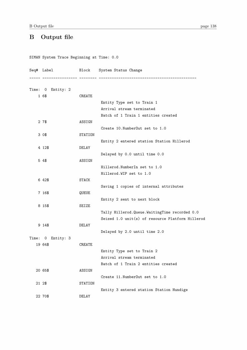
B Output file page 138
B Output file
SIMAN System Trace Beginning at Time: 0.0
Seq# Label Block System Status Change
_____ ________________ ________ _____________________________________________
Time: 0 Entity: 2
1 6$ CREATE
Entity Type set to Train 1
Arrival stream terminated
Batch of 1 Train 1 entities created
2 7$ ASSIGN
Create 10.NumberOut set to 1.0
3 0$ STATION
Entity 2 entered station Station Hillerod
4 12$ DELAY
Delayed by 0.0 until time 0.0
5 4$ ASSIGN
Hillerod.NumberIn set to 1.0
Hillerod.WIP set to 1.0
6 42$ STACK
Saving 1 copies of internal attributes
7 16$ QUEUE
Entity 2 sent to next block
8 15$ SEIZE
Tally Hillerod.Queue.WaitingTime recorded 0.0
Seized 1.0 unit(s) of resource Platform Hillerod
9 14$ DELAY
Delayed by 2.0 until time 2.0
Time: 0 Entity: 3
19 64$ CREATE
Entity Type set to Train 2
Arrival stream terminated
Batch of 1 Train 2 entities created
20 65$ ASSIGN
Create 11.NumberOut set to 1.0
21 2$ STATION
Entity 3 entered station Station Hundige
22 70$ DELAY
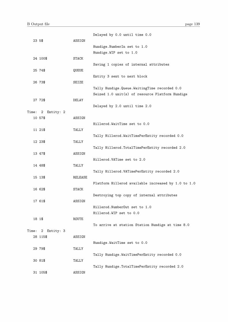
B Output file page 139
Delayed by 0.0 until time 0.0
23 5$ ASSIGN
Hundige.NumberIn set to 1.0
Hundige.WIP set to 1.0
24 100$ STACK
Saving 1 copies of internal attributes
25 74$ QUEUE
Entity 3 sent to next block
26 73$ SEIZE
Tally Hundige.Queue.WaitingTime recorded 0.0
Seized 1.0 unit(s) of resource Platform Hundige
27 72$ DELAY
Delayed by 2.0 until time 2.0
Time: 2 Entity: 2
10 57$ ASSIGN
Hillerod.WaitTime set to 0.0
11 21$ TALLY
Tally Hillerod.WaitTimePerEntity recorded 0.0
12 23$ TALLY
Tally Hillerod.TotalTimePerEntity recorded 2.0
13 47$ ASSIGN
Hillerod.VATime set to 2.0
14 48$ TALLY
Tally Hillerod.VATimePerEntity recorded 2.0
15 13$ RELEASE
Platform Hillerod available increased by 1.0 to 1.0
16 62$ STACK
Destroying top copy of internal attributes
17 61$ ASSIGN
Hillerod.NumberOut set to 1.0
Hillerod.WIP set to 0.0
18 1$ ROUTE
To arrive at station Station Hundige at time 8.0
Time: 2 Entity: 3
28 115$ ASSIGN
Hundige.WaitTime set to 0.0
29 79$ TALLY
Tally Hundige.WaitTimePerEntity recorded 0.0
30 81$ TALLY
Tally Hundige.TotalTimePerEntity recorded 2.0
31 105$ ASSIGN
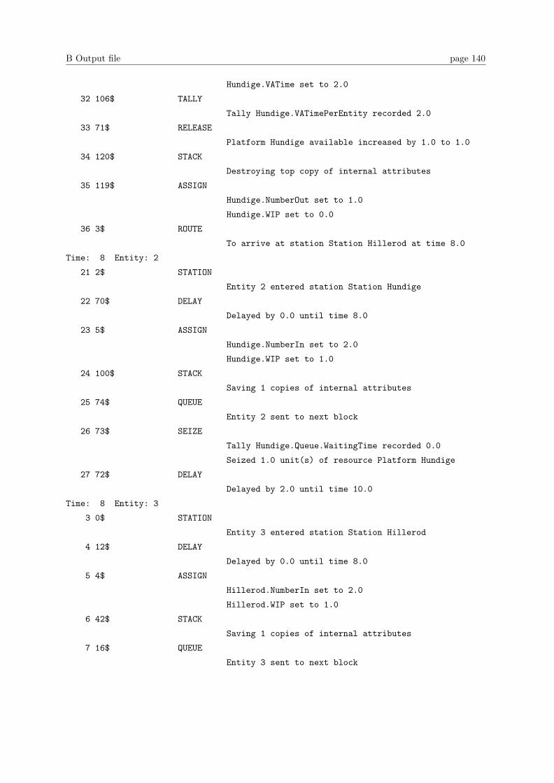
B Output file page 140
Hundige.VATime set to 2.0
32 106$ TALLY
Tally Hundige.VATimePerEntity recorded 2.0
33 71$ RELEASE
Platform Hundige available increased by 1.0 to 1.0
34 120$ STACK
Destroying top copy of internal attributes
35 119$ ASSIGN
Hundige.NumberOut set to 1.0
Hundige.WIP set to 0.0
36 3$ ROUTE
To arrive at station Station Hillerod at time 8.0
Time: 8 Entity: 2
21 2$ STATION
Entity 2 entered station Station Hundige
22 70$ DELAY
Delayed by 0.0 until time 8.0
23 5$ ASSIGN
Hundige.NumberIn set to 2.0
Hundige.WIP set to 1.0
24 100$ STACK
Saving 1 copies of internal attributes
25 74$ QUEUE
Entity 2 sent to next block
26 73$ SEIZE
Tally Hundige.Queue.WaitingTime recorded 0.0
Seized 1.0 unit(s) of resource Platform Hundige
27 72$ DELAY
Delayed by 2.0 until time 10.0
Time: 8 Entity: 3
3 0$ STATION
Entity 3 entered station Station Hillerod
4 12$ DELAY
Delayed by 0.0 until time 8.0
5 4$ ASSIGN
Hillerod.NumberIn set to 2.0
Hillerod.WIP set to 1.0
6 42$ STACK
Saving 1 copies of internal attributes
7 16$ QUEUE
Entity 3 sent to next block

B Output file page 141
8 15$ SEIZE
Tally Hillerod.Queue.WaitingTime recorded 0.0
Seized 1.0 unit(s) of resource Platform Hillerod
9 14$ DELAY
Delayed by 2.0 until time 10.0
Time: 10 Entity: 2
28 115$ ASSIGN
Hundige.WaitTime set to 0.0
29 79$ TALLY
Tally Hundige.WaitTimePerEntity recorded 0.0
30 81$ TALLY
Tally Hundige.TotalTimePerEntity recorded 2.0
31 105$ ASSIGN
Hundige.VATime set to 4.0
32 106$ TALLY
Tally Hundige.VATimePerEntity recorded 2.0
33 71$ RELEASE
Platform Hundige available increased by 1.0 to 1.0
34 120$ STACK
Destroying top copy of internal attributes
35 119$ ASSIGN
Hundige.NumberOut set to 2.0
Hundige.WIP set to 0.0
36 3$ ROUTE
To arrive at station Station Hillerod at time 16.0
Time: 10 Entity: 3
10 57$ ASSIGN
Hillerod.WaitTime set to 0.0
11 21$ TALLY
Tally Hillerod.WaitTimePerEntity recorded 0.0
12 23$ TALLY
Tally Hillerod.TotalTimePerEntity recorded 2.0
13 47$ ASSIGN
Hillerod.VATime set to 4.0
14 48$ TALLY
Tally Hillerod.VATimePerEntity recorded 2.0
15 13$ RELEASE
Platform Hillerod available increased by 1.0 to 1.0
16 62$ STACK
Destroying top copy of internal attributes
17 61$ ASSIGN
B Output file page 142
Hillerod.NumberOut set to 2.0
Hillerod.WIP set to 0.0
18 1$ ROUTE
To arrive at station Station Hundige at time 16.0
ARENA Simulation Results
IMM - License: STUDENT
Summary for Replication 1 of 1
Project: Model 1 Run execution date : 5/17/2005
Analyst: Mads og Line Model revision date: 5/17/2005
Replication ended at time : 10.0 Minutes
Base Time Units: Minutes
Simulation run time: 0.02 minutes.
Simulation run complete.
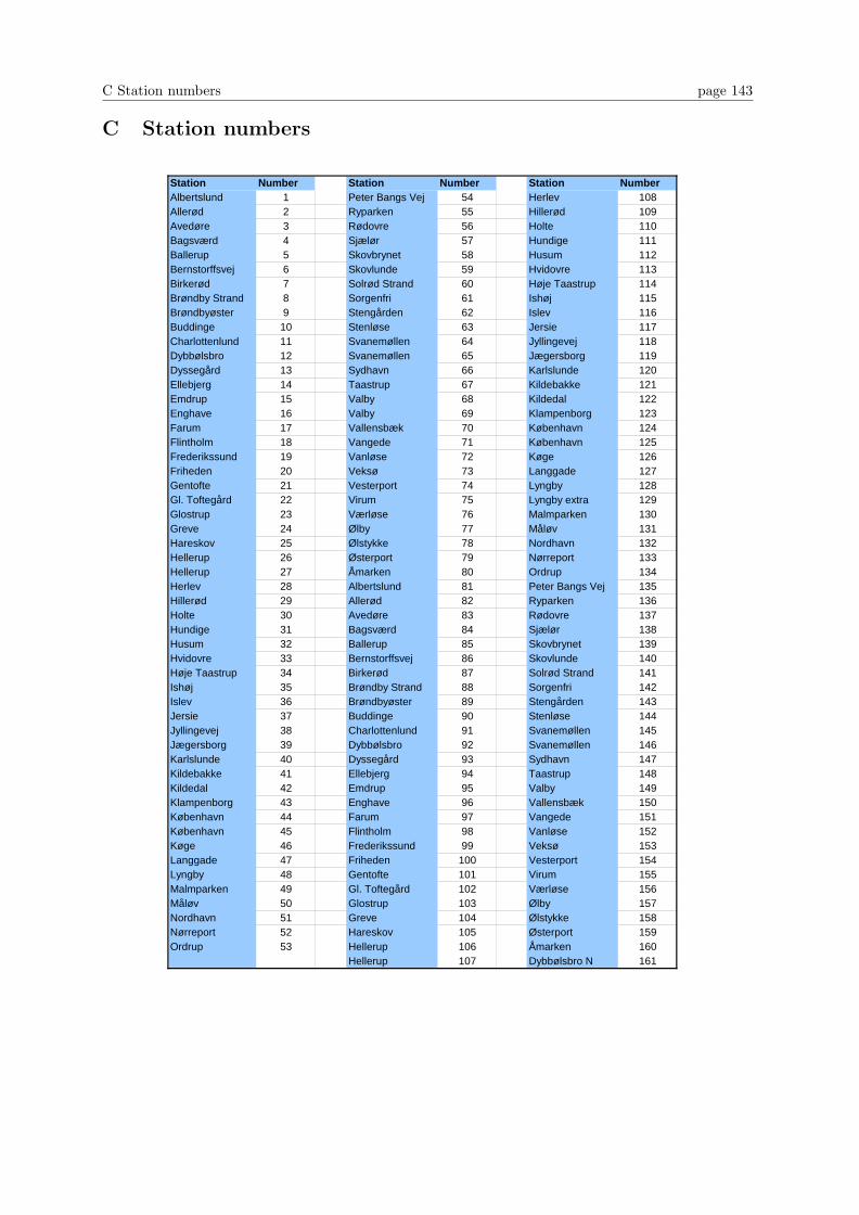
C Station numbers page 143
C Station numbers
Station Number Station Number Station NumberAlbertslund 1 Peter Bangs Vej 54 Herlev 108Allerød 2 Ryparken 55 Hillerød 109Avedøre 3 Rødovre 56 Holte 110Bagsværd 4 Sjælør 57 Hundige 111Ballerup 5 Skovbrynet 58 Husum 112Bernstorffsvej 6 Skovlunde 59 Hvidovre 113Birkerød 7 Solrød Strand 60 Høje Taastrup 114Brøndby Strand 8 Sorgenfri 61 Ishøj 115Brøndbyøster 9 Stengården 62 Islev 116Buddinge 10 Stenløse 63 Jersie 117Charlottenlund 11 Svanemøllen 64 Jyllingevej 118Dybbølsbro 12 Svanemøllen 65 Jægersborg 119Dyssegård 13 Sydhavn 66 Karlslunde 120Ellebjerg 14 Taastrup 67 Kildebakke 121Emdrup 15 Valby 68 Kildedal 122Enghave 16 Valby 69 Klampenborg 123Farum 17 Vallensbæk 70 København 124Flintholm 18 Vangede 71 København 125Frederikssund 19 Vanløse 72 Køge 126Friheden 20 Veksø 73 Langgade 127Gentofte 21 Vesterport 74 Lyngby 128Gl. Toftegård 22 Virum 75 Lyngby extra 129Glostrup 23 Værløse 76 Malmparken 130Greve 24 Ølby 77 Måløv 131Hareskov 25 Ølstykke 78 Nordhavn 132Hellerup 26 Østerport 79 Nørreport 133Hellerup 27 Åmarken 80 Ordrup 134Herlev 28 Albertslund 81 Peter Bangs Vej 135Hillerød 29 Allerød 82 Ryparken 136Holte 30 Avedøre 83 Rødovre 137Hundige 31 Bagsværd 84 Sjælør 138Husum 32 Ballerup 85 Skovbrynet 139Hvidovre 33 Bernstorffsvej 86 Skovlunde 140Høje Taastrup 34 Birkerød 87 Solrød Strand 141Ishøj 35 Brøndby Strand 88 Sorgenfri 142Islev 36 Brøndbyøster 89 Stengården 143Jersie 37 Buddinge 90 Stenløse 144Jyllingevej 38 Charlottenlund 91 Svanemøllen 145Jægersborg 39 Dybbølsbro 92 Svanemøllen 146Karlslunde 40 Dyssegård 93 Sydhavn 147Kildebakke 41 Ellebjerg 94 Taastrup 148Kildedal 42 Emdrup 95 Valby 149Klampenborg 43 Enghave 96 Vallensbæk 150København 44 Farum 97 Vangede 151København 45 Flintholm 98 Vanløse 152Køge 46 Frederikssund 99 Veksø 153Langgade 47 Friheden 100 Vesterport 154Lyngby 48 Gentofte 101 Virum 155Malmparken 49 Gl. Toftegård 102 Værløse 156Måløv 50 Glostrup 103 Ølby 157Nordhavn 51 Greve 104 Ølstykke 158Nørreport 52 Hareskov 105 Østerport 159Ordrup 53 Hellerup 106 Åmarken 160
Hellerup 107 Dybbølsbro N 161
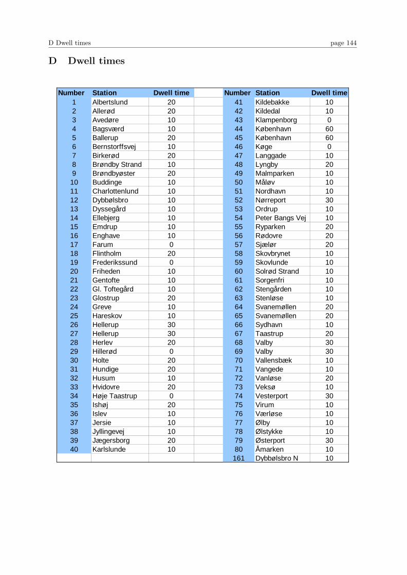
D Dwell times page 144
D Dwell times
Number Station Dwell time Number Station Dwell time1 Albertslund 20 41 Kildebakke 102 Allerød 20 42 Kildedal 103 Avedøre 10 43 Klampenborg 04 Bagsværd 10 44 København 605 Ballerup 20 45 København 606 Bernstorffsvej 10 46 Køge 07 Birkerød 20 47 Langgade 108 Brøndby Strand 10 48 Lyngby 209 Brøndbyøster 20 49 Malmparken 10
10 Buddinge 10 50 Måløv 1011 Charlottenlund 10 51 Nordhavn 1012 Dybbølsbro 10 52 Nørreport 3013 Dyssegård 10 53 Ordrup 1014 Ellebjerg 10 54 Peter Bangs Vej 1015 Emdrup 10 55 Ryparken 2016 Enghave 10 56 Rødovre 2017 Farum 0 57 Sjælør 2018 Flintholm 20 58 Skovbrynet 1019 Frederikssund 0 59 Skovlunde 1020 Friheden 10 60 Solrød Strand 1021 Gentofte 10 61 Sorgenfri 1022 Gl. Toftegård 10 62 Stengården 1023 Glostrup 20 63 Stenløse 1024 Greve 10 64 Svanemøllen 2025 Hareskov 10 65 Svanemøllen 2026 Hellerup 30 66 Sydhavn 1027 Hellerup 30 67 Taastrup 2028 Herlev 20 68 Valby 3029 Hillerød 0 69 Valby 3030 Holte 20 70 Vallensbæk 1031 Hundige 20 71 Vangede 1032 Husum 10 72 Vanløse 2033 Hvidovre 20 73 Veksø 1034 Høje Taastrup 0 74 Vesterport 3035 Ishøj 20 75 Virum 1036 Islev 10 76 Værløse 1037 Jersie 10 77 Ølby 1038 Jyllingevej 10 78 Ølstykke 1039 Jægersborg 20 79 Østerport 3040 Karlslunde 10 80 Åmarken 10
161 Dybbølsbro N 10
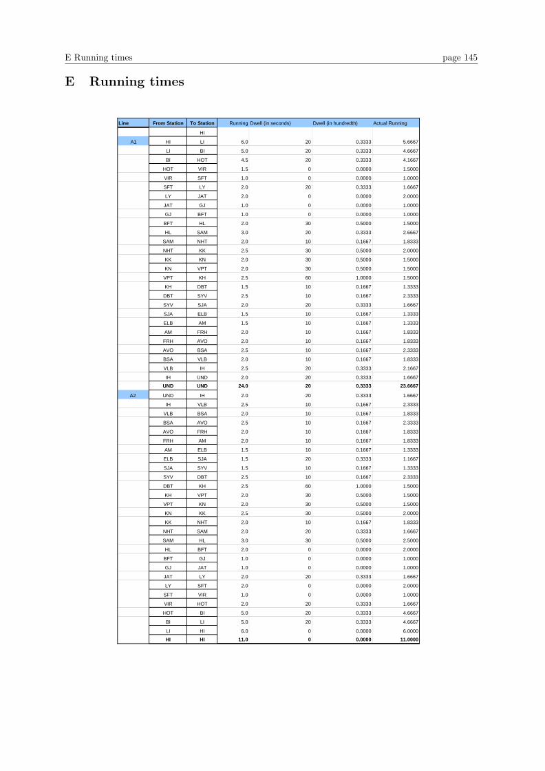
E Running times page 145
E Running times
Line From Station To Station Running Dwell (in seconds) Dwell (in hundredth) Actual Running
HI
A1 HI LI 6.0 20 0.3333 5.6667
LI BI 5.0 20 0.3333 4.6667
BI HOT 4.5 20 0.3333 4.1667
HOT VIR 1.5 0 0.0000 1.5000
VIR SFT 1.0 0 0.0000 1.0000
SFT LY 2.0 20 0.3333 1.6667
LY JAT 2.0 0 0.0000 2.0000
JAT GJ 1.0 0 0.0000 1.0000
GJ BFT 1.0 0 0.0000 1.0000
BFT HL 2.0 30 0.5000 1.5000
HL SAM 3.0 20 0.3333 2.6667
SAM NHT 2.0 10 0.1667 1.8333
NHT KK 2.5 30 0.5000 2.0000
KK KN 2.0 30 0.5000 1.5000
KN VPT 2.0 30 0.5000 1.5000
VPT KH 2.5 60 1.0000 1.5000
KH DBT 1.5 10 0.1667 1.3333
DBT SYV 2.5 10 0.1667 2.3333
SYV SJA 2.0 20 0.3333 1.6667
SJA ELB 1.5 10 0.1667 1.3333
ELB AM 1.5 10 0.1667 1.3333
AM FRH 2.0 10 0.1667 1.8333
FRH AVO 2.0 10 0.1667 1.8333
AVO BSA 2.5 10 0.1667 2.3333
BSA VLB 2.0 10 0.1667 1.8333
VLB IH 2.5 20 0.3333 2.1667
IH UND 2.0 20 0.3333 1.6667
UND UND 24.0 20 0.3333 23.6667
A2 UND IH 2.0 20 0.3333 1.6667
IH VLB 2.5 10 0.1667 2.3333
VLB BSA 2.0 10 0.1667 1.8333
BSA AVO 2.5 10 0.1667 2.3333
AVO FRH 2.0 10 0.1667 1.8333
FRH AM 2.0 10 0.1667 1.8333
AM ELB 1.5 10 0.1667 1.3333
ELB SJA 1.5 20 0.3333 1.1667
SJA SYV 1.5 10 0.1667 1.3333
SYV DBT 2.5 10 0.1667 2.3333
DBT KH 2.5 60 1.0000 1.5000
KH VPT 2.0 30 0.5000 1.5000
VPT KN 2.0 30 0.5000 1.5000
KN KK 2.5 30 0.5000 2.0000
KK NHT 2.0 10 0.1667 1.8333
NHT SAM 2.0 20 0.3333 1.6667
SAM HL 3.0 30 0.5000 2.5000
HL BFT 2.0 0 0.0000 2.0000
BFT GJ 1.0 0 0.0000 1.0000
GJ JAT 1.0 0 0.0000 1.0000
JAT LY 2.0 20 0.3333 1.6667
LY SFT 2.0 0 0.0000 2.0000
SFT VIR 1.0 0 0.0000 1.0000
VIR HOT 2.0 20 0.3333 1.6667
HOT BI 5.0 20 0.3333 4.6667
BI LI 5.0 20 0.3333 4.6667
LI HI 6.0 0 0.0000 6.0000
HI HI 11.0 0 0.0000 11.0000
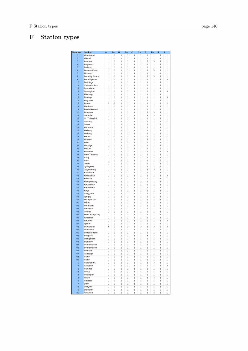
F Station types page 146
F Station types
Nummer Station A A+ B B+ C C+ E E+ F L1 Albertslund 1 1 1 1 1 1 1 1 1 12 Allerød 1 1 1 1 1 1 1 1 1 13 Avedøre 1 1 1 1 1 1 3 3 1 14 Bagsværd 1 1 1 1 1 1 1 1 1 15 Ballerup 1 1 1 1 1 1 1 1 1 16 Bernstorffsvej 1 1 1 1 1 1 3 3 1 17 Birkerød 1 1 1 1 1 1 1 1 1 18 Brøndby Strand 1 1 1 1 1 1 3 3 1 19 Brøndbyøster 1 1 1 1 1 1 1 1 1 310 Buddinge 1 1 1 1 1 1 1 1 1 111 Charlottenlund 1 1 1 1 1 1 1 1 1 112 Dybbølsbro 1 1 1 1 1 1 1 1 1 113 Dyssegård 1 1 1 1 1 1 1 1 1 314 Ellebjerg 1 1 1 1 1 1 1 1 1 115 Emdrup 1 1 1 1 1 1 1 1 1 316 Enghave 1 1 1 1 1 1 1 1 1 117 Farum 2 2 1 1 1 1 1 1 1 218 Flintholm 1 1 1 1 1 1 1 1 1 119 Frederikssund 1 1 1 1 1 1 1 1 1 120 Friheden 1 1 1 1 1 1 3 3 1 121 Gentofte 1 1 1 1 1 1 3 3 1 122 Gl. Toftegård 1 1 1 1 1 1 1 1 1 123 Glostrup 1 1 1 1 1 1 1 1 1 124 Greve 1 1 1 1 1 1 1 1 1 125 Hareskov 1 1 1 1 1 1 1 1 1 126 Hellerup 1 1 1 1 1 1 1 1 1 127 Hellerup 1 1 1 1 1 1 1 1 1 128 Herlev 1 1 1 1 1 1 1 1 1 129 Hillerød 1 1 1 1 1 1 2 2 1 130 Holte 1 1 2 2 1 1 1 1 1 131 Hundige 1 1 1 1 1 1 1 1 1 132 Husum 1 1 1 1 1 1 1 1 3 133 Hvidovre 1 1 1 1 1 1 1 1 1 334 Høje Taastrup 1 1 1 1 1 1 1 1 1 135 Ishøj 1 1 1 1 1 1 1 1 1 136 Islev 1 1 1 1 1 1 1 1 3 137 Jersie 1 1 1 1 1 1 1 1 1 138 Jyllingevej 1 1 1 1 1 1 1 1 3 139 Jægersborg 1 1 1 1 1 1 3 3 1 140 Karlslunde 1 1 1 1 1 1 1 1 1 141 Kildebakke 1 1 1 1 1 1 1 1 1 342 Kildedal 1 1 1 1 1 1 1 1 3 143 Klampenborg 1 1 1 1 2 2 1 1 1 144 København 1 1 1 1 1 1 1 1 1 145 København 1 1 1 1 1 1 1 1 1 146 Køge 1 1 1 1 1 1 1 1 1 147 Langgade 1 1 1 1 1 1 1 1 1 148 Lyngby 1 1 1 1 1 1 1 1 1 149 Malmparken 1 1 1 1 1 1 1 1 3 150 Måløv 1 1 1 1 1 1 1 1 1 151 Nordhavn 1 1 1 1 1 1 1 1 1 152 Nørreport 1 1 1 1 1 1 1 1 1 153 Ordrup 1 1 1 1 1 1 1 1 1 154 Peter Bangs Vej 1 1 1 1 1 1 1 1 1 155 Ryparken 1 1 1 1 1 1 1 1 1 156 Rødovre 1 1 1 1 1 1 1 1 1 357 Sjælør 1 1 1 1 1 1 1 1 1 158 Skovbrynet 3 3 3 3 3 3 3 3 3 359 Skovlunde 1 1 1 1 1 1 1 1 3 160 Solrød Strand 1 1 1 1 1 1 1 1 1 161 Sorgenfri 1 1 1 1 1 1 3 3 1 162 Stengården 1 1 1 1 1 1 1 1 1 163 Stenløse 1 1 1 1 1 1 1 1 1 164 Svanemøllen 1 1 1 1 1 1 1 1 1 165 Svanemøllen 1 1 1 1 1 1 1 1 1 166 Sydhavn 1 1 1 1 1 1 1 1 1 167 Taastrup 1 1 1 1 1 1 1 1 1 168 Valby 1 1 1 1 1 1 1 1 1 169 Valby 1 1 1 1 1 1 1 1 1 170 Vallensbæk 1 1 1 1 1 1 3 3 1 171 Vangede 1 1 1 1 1 1 1 1 1 372 Vanløse 1 1 1 1 1 1 1 1 1 173 Veksø 1 1 1 1 1 1 1 1 1 174 Vesterport 1 1 1 1 1 1 1 1 1 175 Virum 1 1 1 1 1 1 3 3 1 176 Værløse 1 1 1 1 1 1 1 1 1 177 Ølby 1 1 1 1 1 1 1 1 1 178 Ølstykke 1 1 1 1 1 1 1 1 1 179 Østerport 1 1 1 1 1 1 1 1 2 180 Åmarken 1 1 1 1 1 1 3 3 1 1
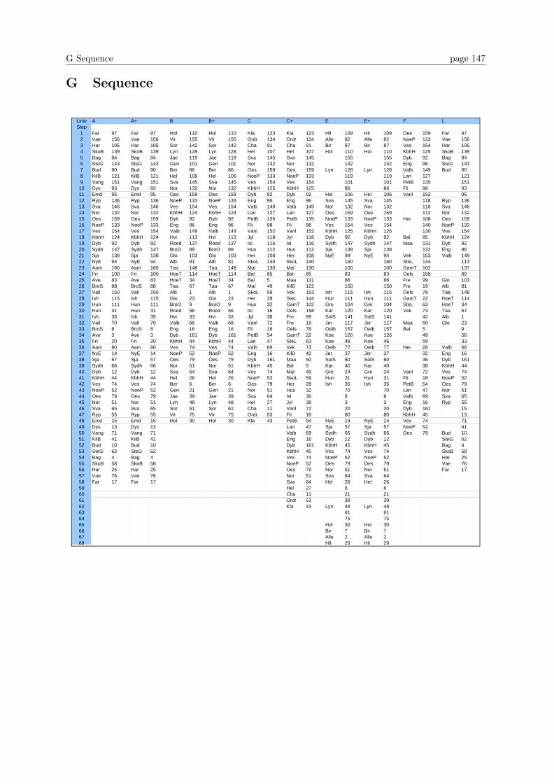
G Sequence page 147
G Sequence
Linie A A+ B B+ C C+ E E+ F LStep
1 Far 97 Far 97 Hol 110 Hol 110 Kla 123 Kla 123 Hil 109 Hil 109 Oes 159 Far 972 Vae 156 Vae 156 Vir 155 Vir 155 Ordr 134 Ordr 134 Alle 82 Alle 82 NoeP 133 Vae 1563 Har 105 Har 105 Sor 142 Sor 142 Cha 91 Cha 91 Bir 87 Bir 87 Ves 154 Har 1054 SkoB 139 SkoB 139 Lyn 128 Lyn 128 Hel 107 Hel 107 Hol 110 Hol 110 KbhH 125 SkoB 1395 Bag 84 Bag 84 Jae 119 Jae 119 Sva 145 Sva 145 155 155 Dyb 92 Bag 846 SteG 143 SteG 143 Gen 101 Gen 101 Nor 132 Nor 132 142 142 Eng 96 SteG 1437 Bud 90 Bud 90 Ber 86 Ber 86 Oes 159 Oes 159 Lyn 128 Lyn 128 Valb 149 Bud 908 KilB 121 KilB 121 Hel 106 Hel 106 NoeP 133 NoeP 133 119 119 Lan 127 1219 Vang 151 Vang 151 Sva 145 Sva 145 Ves 154 Ves 154 101 101 PetB 135 15110 Dys 93 Dys 93 Nor 132 Nor 132 KbhH 125 KbhH 125 86 86 Fli 98 9311 Emd 95 Emd 95 Oes 159 Oes 159 Dyb 92 Dyb 92 Hel 106 Hel 106 Vanl 152 9512 Ryp 136 Ryp 136 NoeP 133 NoeP 133 Eng 96 Eng 96 Sva 145 Sva 145 118 Ryp 13613 Sva 146 Sva 146 Ves 154 Ves 154 Valb 149 Valb 149 Nor 132 Nor 132 116 Sva 14614 Nor 132 Nor 132 KbhH 124 KbhH 124 Lan 127 Lan 127 Oes 159 Oes 159 112 Nor 13215 Oes 159 Oes 159 Dyb 92 Dyb 92 PetB 135 PetB 135 NoeP 133 NoeP 133 Her 108 Oes 15916 NoeP 133 NoeP 133 Eng 96 Eng 96 Fli 98 Fli 98 Ves 154 Ves 154 140 NoeP 13317 Ves 154 Ves 154 Valb 149 Valb 149 Vanl 152 Vanl 152 KbhH 125 KbhH 125 130 Ves 15418 KbhH 124 KbhH 124 Hvi 113 Hvi 113 Jyl 118 Jyl 118 Dyb 92 Dyb 92 Bal 85 KbhH 12419 Dyb 92 Dyb 92 Roed 137 Roed 137 Isl 116 Isl 116 Sydh 147 Sydh 147 Maa 131 Dyb 9220 Sydh 147 Sydh 147 BroO 89 BroO 89 Hus 112 Hus 112 Sja 138 Sja 138 122 Eng 9621 Sja 138 Sja 138 Glo 103 Glo 103 Her 108 Her 108 NyE 94 NyE 94 Vek 153 Valb 14922 NyE 94 NyE 94 Alb 81 Alb 81 SkoL 140 SkoL 140 160 160 SteL 144 11323 Aam 160 Aam 160 Taa 148 Taa 148 Mal 130 Mal 130 100 100 GamT 102 13724 Fri 100 Fri 100 HoeT 114 HoeT 114 Bal 85 Bal 85 83 83 Oels 158 8925 Ave 83 Ave 83 HoeT 34 HoeT 34 Bal 5 Maa 131 88 88 Fre 99 Glo 10326 BroS 88 BroS 88 Taa 67 Taa 67 Mal 49 KilD 122 150 150 Fre 19 Alb 8127 Vall 150 Vall 150 Alb 1 Alb 1 SkoL 59 Vek 153 Ish 115 Ish 115 Oels 78 Taa 14828 Ish 115 Ish 115 Glo 23 Glo 23 Her 28 SteL 144 Hun 111 Hun 111 GamT 22 HoeT 11429 Hun 111 Hun 111 BroO 9 BroO 9 Hus 32 GamT 102 Gre 104 Gre 104 SteL 63 HoeT 3430 Hun 31 Hun 31 Roed 56 Roed 56 Isl 36 Oels 158 Kar 120 Kar 120 Vek 73 Taa 6731 Ish 35 Ish 35 Hvi 33 Hvi 33 Jyl 38 Fre 99 SolS 141 SolS 141 42 Alb 132 Vall 70 Vall 70 Valb 68 Valb 68 Vanl 72 Fre 19 Jer 117 Jer 117 Maa 50 Glo 2333 BroS 8 BroS 8 Eng 16 Eng 16 Fli 18 Oels 78 Oelb 157 Oelb 157 Bal 5 934 Ave 3 Ave 3 Dyb 161 Dyb 161 PetB 54 GamT 22 Koe 126 Koe 126 49 5635 Fri 20 Fri 20 KbhH 44 KbhH 44 Lan 47 SteL 63 Koe 46 Koe 46 59 3336 Aam 80 Aam 80 Ves 74 Ves 74 Valb 69 Vek 73 Oelb 77 Oelb 77 Her 28 Valb 6837 NyE 14 NyE 14 NoeP 52 NoeP 52 Eng 16 KilD 42 Jer 37 Jer 37 32 Eng 1638 Sja 57 Sja 57 Oes 79 Oes 79 Dyb 161 Maa 50 SolS 60 SolS 60 36 Dyb 16139 Sydh 66 Sydh 66 Nor 51 Nor 51 KbhH 45 Bal 5 Kar 40 Kar 40 38 KbhH 4440 Dyb 12 Dyb 12 Sva 64 Sva 64 Ves 74 Mal 49 Gre 24 Gre 24 Vanl 72 Ves 7441 KbhH 44 KbhH 44 Hel 26 Hel 26 NoeP 52 SkoL 59 Hun 31 Hun 31 Fli 18 NoeP 5242 Ves 74 Ves 74 Ber 6 Ber 6 Oes 79 Her 28 Ish 35 Ish 35 PetB 54 Oes 7943 NoeP 52 NoeP 52 Gen 21 Gen 21 Nor 51 Hus 32 70 70 Lan 47 Nor 5144 Oes 79 Oes 79 Jae 39 Jae 39 Sva 64 Isl 36 8 8 Valb 69 Sva 6545 Nor 51 Nor 51 Lyn 48 Lyn 48 Hel 27 Jyl 38 3 3 Eng 16 Ryp 5546 Sva 65 Sva 65 Sor 61 Sor 61 Cha 11 Vanl 72 20 20 Dyb 161 1547 Ryp 55 Ryp 55 Vir 75 Vir 75 Ordr 53 Fli 18 80 80 KbhH 45 1348 Emd 15 Emd 15 Hol 30 Hol 30 Kla 43 PetB 54 NyE 14 NyE 14 Ves 74 7149 Dys 13 Dys 13 Lan 47 Sja 57 Sja 57 NoeP 52 4150 Vang 71 Vang 71 Valb 69 Sydh 66 Sydh 66 Oes 79 Bud 1051 KilB 41 KilB 41 Eng 16 Dyb 12 Dyb 12 SteG 6252 Bud 10 Bud 10 Dyb 161 KbhH 45 KbhH 45 Bag 453 SteG 62 SteG 62 KbhH 45 Ves 74 Ves 74 SkoB 5854 Bag 4 Bag 4 Ves 74 NoeP 52 NoeP 52 Har 2555 SkoB 58 SkoB 58 NoeP 52 Oes 79 Oes 79 Vae 7656 Har 25 Har 25 Oes 79 Nor 51 Nor 51 Far 1757 Vae 76 Vae 76 Nor 51 Sva 64 Sva 6458 Far 17 Far 17 Sva 64 Hel 26 Hel 2659 Hel 27 6 660 Cha 11 21 2161 Ordr 53 39 3962 Kla 43 Lyn 48 Lyn 4863 61 6164 75 7565 Hol 30 Hol 3066 Bir 7 Bir 767 Alle 2 Alle 268 Hil 29 Hil 29
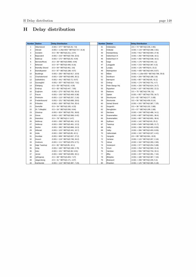
H Delay distribution page 148
H Delay distribution
Number Station Delay Distribution Number Station Delay Distribution
1 Albertslund -0.001 + 277 * BETA(0.26, 7.9) 41 Kildebakke -0.5 + 74 * BETA(0.226, 2.85)
2 Allerød -0.001 + 1.26e+003 * BETA(0.717, 31.8) 42 Kildedal -0.001 + 119 * BETA(0.288, 2.81)
3 Avedøre -0.5 + 95 * BETA(0.211, 2.07) 43 Klampenborg -0.001 + 912 * BETA(0.664, 27.8)
4 Bagsværd -0.001 + 215 * BETA(0.728, 32.6) 44 København H -0.001 + 292 * BETA(0.538, 18.1)
5 Ballerup -0.001 + 172 * BETA(0.25, 4.04) 45 København H -0.001 + 292 * BETA(0.538, 18.1)
6 Bernstorffsvej -0.5 + 39 * BETA(0.0908, 4.94) 46 Køge -0.001 + 176 * BETA(0.444, 11)
7 Birkerød -0.5 + 97 * BETA(0.406, 8.16) 47 Langgade -0.001 + 215 * BETA(0.367, 6.3)
8 Brøndby Strand -0.5 + 94 * BETA(0.461, 3.8) 48 Lyngby -0.001 + 126 * BETA(0.5, 15.2)
9 Brøndbyøster -0.5 + 87 * BETA(0.188, 4.07) 49 Malmparken -0.001 + 439 * BETA(0.404, 8.07)
10 Buddinge -0.001 + 265 * BETA(0.917, 10.9) 50 Måløv -0.001 + 1.16e+003 * BETA(0.766, 35.6)
11 Charlottenlund -0.001 + 158 * BETA(0.695, 30.2) 51 Nordhavn -0.001 + 204 * BETA(0.188, 3.9)
12 Dybbølsbro -0.001 + 441 * BETA(0.72, 9.07) 52 Nørreport -0.001 + 807 * BETA(0.85, 42.1)
13 Dyssegård -0.001 + 307 * BETA(0.519, 7.51) 53 Ordrup -0.001 + 174 * BETA(0.751, 4.7)
14 Ellebjerg -0.5 + 59 * BETA(0.82, 4.36) 54 Peter Bangs Vej -0.001 + 200 * BETA(0.624, 24.7)
15 Emdrup -0.5 + 65 * BETA(0.447, 7.95) 55 Ryparken -0.001 + 187 * BETA(0.592, 22.2)
16 Enghave -0.001 + 270 * BETA(0.763, 35.4) 56 Rødovre -0.5 + 75 * BETA(0.706, 31)
17 Farum -0.001 + 193 * BETA(0.409, 8.38) 57 Sjælør -0.001 + 957 * BETA(0.755, 34.7)
18 Flintholm -0.001 + 115 * BETA(0.267, 2.16) 58 Skovbrynet -0.5 + 82 * BETA(0.277, 5.08)
19 Frederikssund -0.001 + 151 * BETA(0.688, 29.6) 59 Skovlunde -0.5 + 56 * BETA(0.459, 8.14)
20 Friheden -0.001 + 300 * BETA(0.764, 35.4) 60 Solrød Strand -0.001 + 243 * BETA(0.387, 7.25)
21 Gentofte -0.5 + 34 * BETA(0.165, 4.23) 61 Sorgenfri -0.5 + 36 * BETA(0.152, 3.88)
22 Gl. Toftegård -0.5 + 54 * BETA(0.556, 9.64) 62 Stengården -0.5 + 57 * BETA(0.199, 2.68)
23 Glostrup -0.001 + 824 * BETA(0.781, 36.8) 63 Stenløse -0.001 + 240 * BETA(0.486, 14.1)
24 Greve -0.001 + 162 * BETA(0.568, 6.42) 64 Svanemøllen -0.001 + 687 * BETA(0.801, 38.4)
25 Hareskov -0.5 + 78 * BETA(2.4, 5.47) 65 Svanemøllen -0.001 + 687 * BETA(0.801, 38.4)
26 Hellerup -0.001 + 265 * BETA(0.461, 12.3) 66 Sydhavn -0.001 + 142 * BETA(0.63, 25.1)
27 Hellerup -0.001 + 265 * BETA(0.461, 12.3) 67 Taastrup -0.001 + 549 * BETA(0.585, 21.7)
28 Herlev -0.001 + 382 * BETA(0.868, 15.3) 68 Valby -0.001 + 266 * BETA(0.403, 8.05)
29 Hillerød -0.001 + 123 * BETA(0.441, 10.7) 69 Valby -0.001 + 266 * BETA(0.403, 8.05)
30 Holte -0.001 + 265 * BETA(0.85, 42.1) 70 Vallensbæk -0.001 + 102 * BETA(0.327, 4.41)
31 Hundige -0.001 + 606 * BETA(0.657, 27.2) 71 Vangede -0.5 + 89 * BETA(0.561, 19.9)
32 Husum -0.001 + 119 * BETA(0.748, 34.2) 72 Vanløse -0.001 + 115 * BETA(0.267, 2.16)
33 Hvidovre -0.001 + 111 * BETA(0.376, 6.71) 73 Veksø -0.001 + 162 * BETA(0.283, 2.65)
34 Høje Taastrup -0.5 + 82 * BETA(0.85, 42.1) 74 Vesterport -0.001 + 377 * BETA(0.254, 5.68)
35 Ishøj -0.001 + 160 * BETA(0.168, 2.79) 75 Virum -0.001 + 254 * BETA(0.583, 21.6)
36 Islev -0.001 + 101 * BETA(0.38, 6.91) 76 Værløse -0.001 + 556 * BETA(0.734, 33.1)
37 Jersie -0.001 + 646 * BETA(0.695, 30.1) 77 Ølby -0.001 + 207 * BETA(0.391, 7.44)
38 Jyllingevej -0.5 + 68 * BETA(0.403, 7.27) 78 Ølstykke -0.001 + 188 * BETA(0.387, 7.24)
39 Jægersborg -0.5 + 31 * BETA(0.171, 4.07) 79 Østerport -0.001 + 208 * BETA(0.205, 5.3)
40 Karlslunde -0.001 + 110 * BETA(0.387, 7.23) 80 Åmarken -0.001 + 125 * BETA(0.365, 6.18)
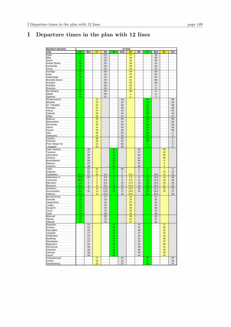
I Departure times in the plan with 12 lines page 149
I Departure times in the plan with 12 lines
Northern directionLine A Bxx C+ Ax B Cxx A+ Bx C Axx B+ CxKøge 17 22 27 32Ølby 20 25 30 35Jersie 24 29 34 39Solrød Strand 26 31 36 41Karlslunde 29 34 39 44Greve 32 37 42 47Hundige 34 39 44 49Ishøj 37 42 47 52Vallensbæk 39 44 49 54Brøndby Strand 41 46 51 56Avedøre 43 48 53 58Friheden 45 50 55 0Åmarken 47 52 57 2Ny Ellebjerg 49 54 59 4Sjælør 51 56 1 6Sydhavn 52 57 2 7Frederikssund 13 18 23 28Ølstykke 19 24 29 34Gl. Toftegård 21 26 31 36Stenløse 23 28 33 38Veksø 27 32 37 42Kildedal 29 34 39 44Måløv 32 37 42 47Ballerup 35 40 45 50Malmparken 37 42 47 52Skovlunde 39 44 49 54Herlev 41 46 51 56Husum 43 48 53 58Islev 45 50 55 0Jyllingevej 47 52 57 2Vanløse 48 53 58 3Flintholm 49 54 59 4Peter Bangs Vej 51 56 1 6Langgade 53 58 3 8Høje Taastrup 35 40 45 50Taastrup 37 42 47 52Albertslund 40 45 50 55Glostrup 43 48 53 58Brøndbyøster 45 50 55 0Rødovre 47 52 57 2Hvidovre 49 54 59 4Valby 52 54 57 59 2 4 7 9Enghave 55 57 0 2 5 7 10 12Dybbølsbro 55.5 57 59 0.5 2 4 5.5 7 9 10.5 12 14København H 57.5 59 1 2.5 4 6 7.5 9 11 12.5 14 16Vesterport 59.5 1 3 4.5 6 8 9.5 11 13 14.5 16 18Nørreport 1.5 3 5 6.5 8 10 11.5 13 15 16.5 18 20Østerport 4.5 6 8 9.5 11 13 14.5 16 18 19.5 21 23Nordhavn 6.5 8 10 11.5 13 15 16.5 18 20 21.5 23 25Svanemøllen 8.5 10 12 13.5 15 17 18.5 20 22 23.5 25 27Hellerup 10.5 14 15.5 19 20.5 24 25.5 29Bernstorffsvej 12 17 22 27Gentofte 14 19 24 29Jægersborg 16 21 26 31Lyngby 18 23 28 33Sorgenfri 20 25 30 35Virum 22 27 32 37Holte 24 29 34 39Birkerød 28 33 38 43Allerød 32 37 42 47Hillerød 37 42 47 52Ryparken 12 17 22 27Emdrup 14 19 24 29Dyssegård 16 21 26 31Vangede 17 22 27 32Kildebakke 19 24 29 34Buddinge 21 26 31 36Stengården 22 27 32 37Bagsværd 24 29 34 39Skovbrynet 26 31 36 41Hareskov 28 33 38 43Værløse 30 35 40 45Farum 34 39 44 49Charlottenlund 17 22 27 32Ordrup 19 24 29 34Klampenborg 22 27 32 37
12 lines

I Departure times in the plan with 12 lines page 150
Southern directionLine C Bxx A+ Cx B Axx C+ Bx A Cxx B+ AxKlampenborg 35 40 45 50Ordrup 38 43 48 53Charlottenlund 40 45 50 55Farum 23 28 33 38Værløse 27 32 37 42Hareskov 29 34 39 44Skovbrynet 31 36 41 46Bagsværd 33 38 43 48Stengården 35 40 45 50Buddinge 36 41 46 51Kildebakke 38 43 48 53Vangede 40 45 50 55Dyssegård 41 46 51 56Emdrup 43 48 53 58Ryparken 45 50 55 0Hillerød 20 25 30 35Allerød 25 30 35 40Birkerød 29 34 39 44Holte 33 38 43 48Virum 35 40 45 50Sorgenfri 37 42 47 52Lyngby 39 44 49 54Jægersborg 41 46 51 56Gentofte 43 48 53 58Bernstorffsvej 45 50 55 0Hellerup 43.5 47 48.5 52 53.5 57 58.5 2Svanemøllen 45.5 47 49 50.5 52 54 55.5 57 59 0.5 2 4Nordhavn 47.5 49 51 52.5 54 56 57.5 59 1 2.5 4 6Østerport 49.5 51 53 54.5 56 58 59.5 1 3 4.5 6 8Nørreport 52.5 54 56 57.5 59 1 2.5 4 6 7.5 9 11Vesterport 54.5 56 58 59.5 1 3 4.5 6 8 9.5 11 13København H 56.5 58 0 1.5 3 5 6.5 8 10 11.5 13 15Dybbølsbro 58.5 0 2 3.5 5 7 8.5 10 12 13.5 15 17Enghave 0 2 5 7 10 12 15 17Valby 3 5 8 10 13 15 18 20Hvidovre 8 13 18 23Rødovre 10 15 20 25Brøndbyøster 12 17 22 27Glostrup 14 19 24 29Albertslund 17 22 27 32Taastrup 20 25 30 35Høje Taastrup 22 27 32 37Langgade 4 9 14 19Peter Bangs Vej 6 11 16 21Flintholm 8 13 18 23Vanløse 9 14 19 24Jyllingevej 10 15 20 25Islev 12 17 22 27Husum 14 19 24 29Herlev 16 21 26 31Skovlunde 18 23 28 33Malmparken 20 25 30 35Ballerup 22 27 32 37Måløv 25 30 35 40Kildedal 28 33 38 43Veksø 30 35 40 45Stenløse 34 39 44 49Gl. Toftegård 36 41 46 51Ølstykke 38 43 48 53Frederikssund 44 49 54 59Sydhavn 5 10 15 20Sjælør 6 11 16 21Ny Ellebjerg 8 13 18 23Åmarken 10 15 20 25Friheden 12 17 22 27Avedøre 14 19 24 29Brøndby Strand 16 21 26 31Vallensbæk 18 23 28 33Ishøj 20 25 30 35Hundige 23 28 33 38Greve 25 30 35 40Karlslunde 28 33 38 43Solrød Strand 31 36 41 46Jersie 33 38 43 48Ølby 37 42 47 52Køge 40 45 50 55
12 lines
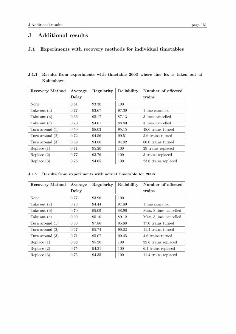
J Additional results page 151
J Additional results
J.1 Experiments with recovery methods for individual timetables
J.1.1 Results from experiments with timetable 2003 where line Ex is taken out at
København
Recovery Method Average
Delay
Regularity Reliability Number of affected
trains
None 0.81 93.30 100
Take out (a) 0.77 93.67 97.39 1 line cancelled
Take out (b) 0.66 95.17 87.13 3 lines cancelled
Take out (c) 0.70 94.61 88.80 3 lines cancelled
Turn around (1) 0.59 98.03 95.15 48.6 trains turned
Turn around (2) 0.72 94.56 99.51 5.6 trains turned
Turn around (3) 0.69 94.80 94.92 60.0 trains turned
Replace (1) 0.71 95.20 100 29 trains replaced
Replace (2) 0.77 93.76 100 3 trains replaced
Replace (3) 0.75 94.65 100 23.6 trains replaced
J.1.2 Results from experiments with actual timetable for 2006
Recovery Method Average
Delay
Regularity Reliability Number of affected
trains
None 0.77 93.96 100
Take out (a) 0.73 94.44 97.89 1 line cancelled
Take out (b) 0.70 95.09 88.96 Max. 3 lines cancelled
Take out (c) 0.69 95.10 89.12 Max. 3 lines cancelled
Turn around (1) 0.58 97.86 95.88 37.0 trains turned
Turn around (2) 0.67 95.74 99.02 11.4 trains turned
Turn around (3) 0.71 95.07 99.45 4.6 trains turned
Replace (1) 0.68 95.20 100 22.6 trains replaced
Replace (2) 0.75 94.31 100 6.4 trains replaced
Replace (3) 0.75 94.35 100 11.4 trains replaced

J.1 Experiments with recovery methods for individual timetables page 152
J.1.3 Results from experiments with actual timetable for 2006 and line Ex taken out
at København
Recovery Method Average
Delay
Regularity Reliability Number of affected
trains
None 0.64 96.10 100
Take out (a) 0.64 96.10 100
Take out (b) 0.64 96.10 100
Turn around (1) 0.54 98.00 96.45 35.4 trains turned
Turn around (2) 0.59 96.86 99.50 4.0 trains turned
Turn around (3) 0.58 96.64 97.17 22.4 trains turned
Replace (1) 0.56 97.48 100 14 trains replaced
Replace (2) 0.64 96.08 100 1.4 trains replaced
Replace (3) 0.63 96.15 100 12.8 trains replaced
J.1.4 Results from experiments with proposed timetable with 10 lines and line G ter-
minating in Buddinge
Recovery Method Average
Delay
Regularity Reliability Number of affected
trains
None 1.22 87.54 100
Take out (a) 1.05 89.59 94.51 Max. 2 lines cancelled
Take out (b) 0.81 93.06 82.01 Max. 3 lines cancelled
Take out (c) 0.80 93.31 83.26 Max. 3 lines cancelled
Turn around (1) 0.67 97.16 94.56 55.8 trains turned
Turn around (2) 0.84 92.86 99.00 10.2 trains turned
Turn around (3) 0.67 95.82 85.70 101.4 trains turned
Replace (1) 0.86 92.89 100 45.4 trains replaced
Replace (2) 0.92 91.35 100 6 trains replaced
Replace (3) 0.88 92.22 100 56 trains replaced
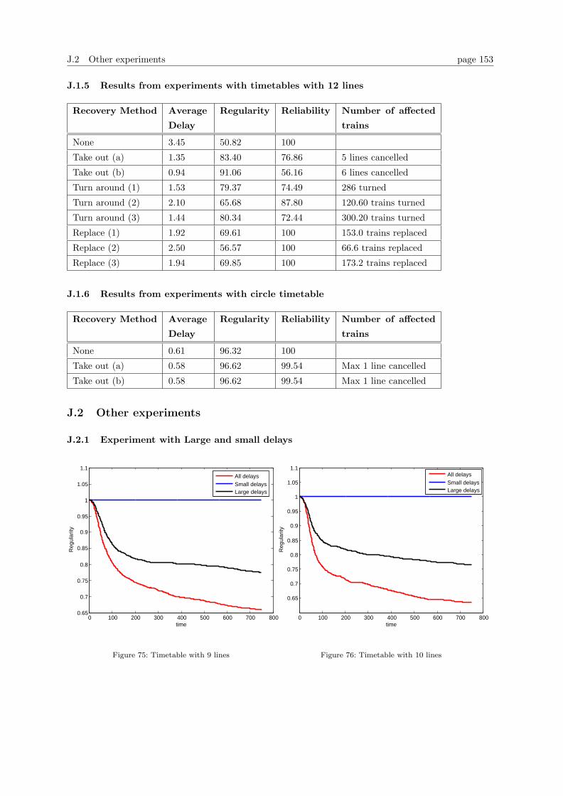
J.2 Other experiments page 153
J.1.5 Results from experiments with timetables with 12 lines
Recovery Method Average
Delay
Regularity Reliability Number of affected
trains
None 3.45 50.82 100
Take out (a) 1.35 83.40 76.86 5 lines cancelled
Take out (b) 0.94 91.06 56.16 6 lines cancelled
Turn around (1) 1.53 79.37 74.49 286 turned
Turn around (2) 2.10 65.68 87.80 120.60 trains turned
Turn around (3) 1.44 80.34 72.44 300.20 trains turned
Replace (1) 1.92 69.61 100 153.0 trains replaced
Replace (2) 2.50 56.57 100 66.6 trains replaced
Replace (3) 1.94 69.85 100 173.2 trains replaced
J.1.6 Results from experiments with circle timetable
Recovery Method Average
Delay
Regularity Reliability Number of affected
trains
None 0.61 96.32 100
Take out (a) 0.58 96.62 99.54 Max 1 line cancelled
Take out (b) 0.58 96.62 99.54 Max 1 line cancelled
J.2 Other experiments
J.2.1 Experiment with Large and small delays
0 100 200 300 400 500 600 700 8000.65
0.7
0.75
0.8
0.85
0.9
0.95
1
1.05
1.1
time
Reg
ular
ity
All delaysSmall delaysLarge delays
Figure 75: Timetable with 9 lines
0 100 200 300 400 500 600 700 800
0.65
0.7
0.75
0.8
0.85
0.9
0.95
1
1.05
1.1
time
Reg
ular
ity
All delaysSmall delaysLarge delays
Figure 76: Timetable with 10 lines
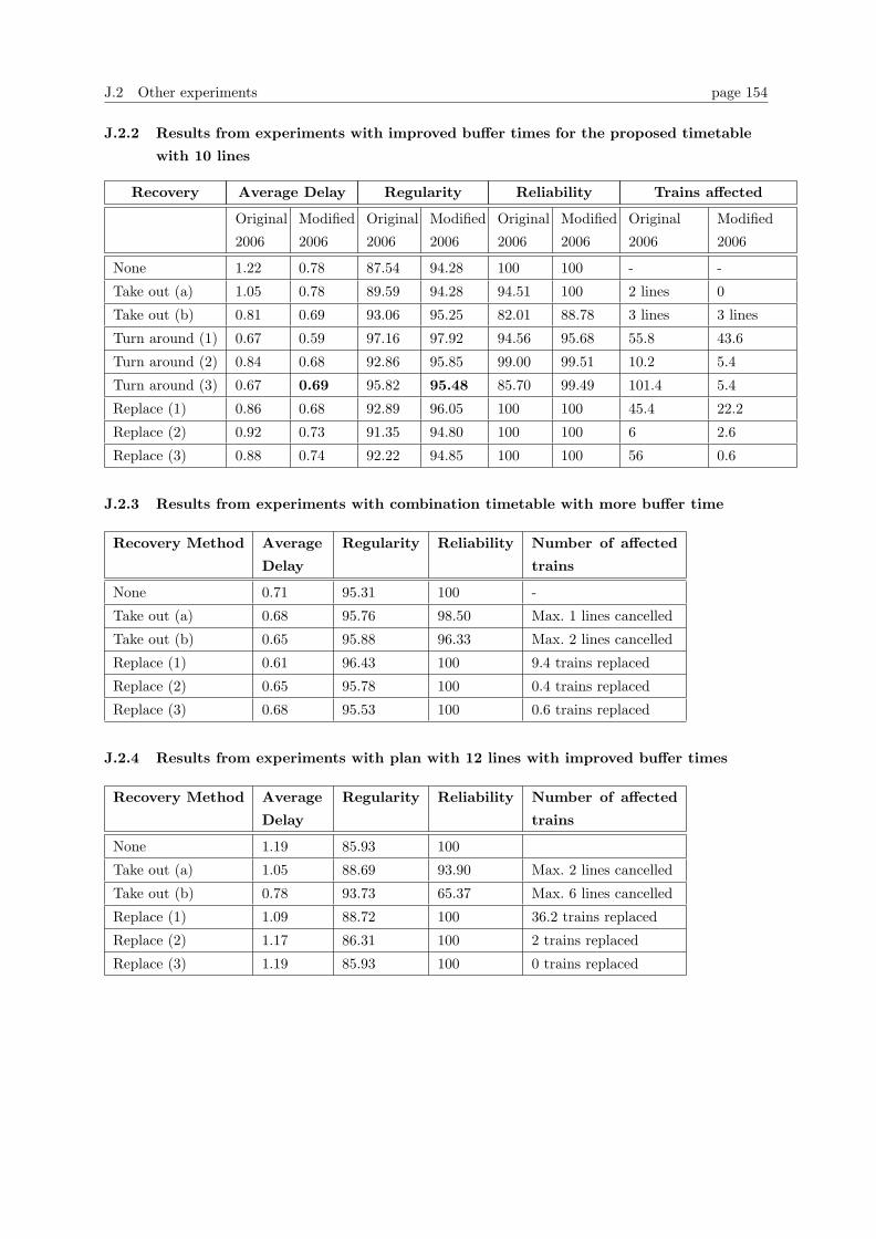
J.2 Other experiments page 154
J.2.2 Results from experiments with improved buffer times for the proposed timetable
with 10 lines
Recovery Average Delay Regularity Reliability Trains affected
Original
2006
Modified
2006
Original
2006
Modified
2006
Original
2006
Modified
2006
Original
2006
Modified
2006
None 1.22 0.78 87.54 94.28 100 100 - -
Take out (a) 1.05 0.78 89.59 94.28 94.51 100 2 lines 0
Take out (b) 0.81 0.69 93.06 95.25 82.01 88.78 3 lines 3 lines
Turn around (1) 0.67 0.59 97.16 97.92 94.56 95.68 55.8 43.6
Turn around (2) 0.84 0.68 92.86 95.85 99.00 99.51 10.2 5.4
Turn around (3) 0.67 0.69 95.82 95.48 85.70 99.49 101.4 5.4
Replace (1) 0.86 0.68 92.89 96.05 100 100 45.4 22.2
Replace (2) 0.92 0.73 91.35 94.80 100 100 6 2.6
Replace (3) 0.88 0.74 92.22 94.85 100 100 56 0.6
J.2.3 Results from experiments with combination timetable with more buffer time
Recovery Method Average
Delay
Regularity Reliability Number of affected
trains
None 0.71 95.31 100 -
Take out (a) 0.68 95.76 98.50 Max. 1 lines cancelled
Take out (b) 0.65 95.88 96.33 Max. 2 lines cancelled
Replace (1) 0.61 96.43 100 9.4 trains replaced
Replace (2) 0.65 95.78 100 0.4 trains replaced
Replace (3) 0.68 95.53 100 0.6 trains replaced
J.2.4 Results from experiments with plan with 12 lines with improved buffer times
Recovery Method Average
Delay
Regularity Reliability Number of affected
trains
None 1.19 85.93 100
Take out (a) 1.05 88.69 93.90 Max. 2 lines cancelled
Take out (b) 0.78 93.73 65.37 Max. 6 lines cancelled
Replace (1) 1.09 88.72 100 36.2 trains replaced
Replace (2) 1.17 86.31 100 2 trains replaced
Replace (3) 1.19 85.93 100 0 trains replaced
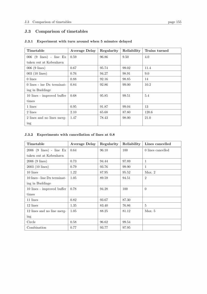
J.3 Comparison of timetables page 155
J.3 Comparison of timetables
J.3.1 Experiment with turn around when 5 minutes delayed
Timetable Average Delay Regularity Reliability Trains turned
006 (9 lines) - line Ex
taken out at København
0.59 96.86 9.50 4.0
006 (9 lines) 0.67 95.74 99.02 11.4
003 (10 lines) 0.76 94.27 98.91 9.0
0 lines 0.88 92.16 98.85 14
0 lines - ine Dx terminat-
ing in Buddinge
0.84 92.86 99.00 10.2
10 lines - improved buffer
times
0.68 95.85 99.51 5.4
1 lines 0.95 91.87 99.04 13
2 lines 2.10 65.68 87.80 120.6
2 lines and no lines merg-
ing
1.47 78.43 98.00 21.0
J.3.2 Experiments with cancellation of lines at 0.8
Timetable Average Delay Regularity Reliability Lines cancelled
2006 (9 lines) - line Ex
taken out at København
0.64 96.10 100 0 lines cancelled
2006 (9 lines) 0.73 94.44 97.89 1
2003 (10 lines) 0.79 93.76 99.90 1
10 lines 1.22 87.95 95.52 Max. 2
10 lines - line Dx terminat-
ing in Buddinge
1.05 89.59 94.51 2
10 lines - improved buffer
times
0.78 94.28 100 0
11 lines 0.82 93.67 87.30
12 lines 1.35 83.40 76.86 5
12 lines and no line merg-
ing
1.05 88.25 81.12 Max. 5
Circle 0.58 96.62 99.54
Combination 0.77 93.77 97.95
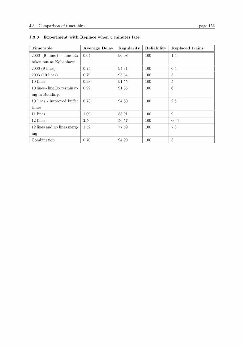
J.3 Comparison of timetables page 156
J.3.3 Experiment with Replace when 5 minutes late
Timetable Average Delay Regularity Reliability Replaced trains
2006 (9 lines) - line Ex
taken out at København
0.64 96.08 100 1.4
2006 (9 lines) 0.75 94.31 100 6.4
2003 (10 lines) 0.79 93.34 100 3
10 lines 0.93 91.55 100 5
10 lines - line Dx terminat-
ing in Buddinge
0.92 91.35 100 6
10 lines - improved buffer
times
0.73 94.80 100 2.6
11 lines 1.09 88.91 100 9
12 lines 2.50 56.57 100 66.6
12 lines and no lines merg-
ing
1.52 77.59 100 7.8
Combination 0.70 94.90 100 3
References
References
[1] Abbink, Von Der Berg, Kroon and Salomon Allocation of Railway Rolling Stock for Passenger
Trains, Transportation Science vol. 38 No. 1pp. 33-41, February 2004.
[2] Alfieri, Groot, Kroon and Schrijver Efficient Circulation of Railway Rolling Stock, ERIM Research
Report ERS-2002-110-LIS, Erasmus University Rotterdam, 2002.
[3] Carey and Malachy Ex ante heuristic measures of schedule reliability, Transportation Research
Part B 33(7), pp. 473-494, 1999.
[4] Carey and Carville Testing schedule performance and reliability for train stations, journal of
Operational Research Society 51, pp. 666-682, 2000.
[5] DSB S-tog Annual Report 2003,
http://www.dsb.dk/servlet/Satellite?pagename=Millenium%2FPage%2FStandardForside&c=Page&cid=1002716363235
date 01-03-2005.
[6] Engelhardt-Funke and Kolonko Analysing stability and investments in railway networks using
advanced evolutionary algorithms, International Transactions In Operational Research 11 pp.
382-394 , 2004.
[7] Goodman and Takagi Dynamic re-scheduling of trains after disruption, Computers in Railways
IX, WIT Press, 2004.
[8] Goverde and Odijk Performance evaluation of network timetables using PETER, Computers in
Railways VIII, WIT Press, 2002.
[9] Hallowell and Harker Predicting on-time performance in scheduled railroad operations: method-
ology and application to train scheduling, Transportation Research Part A: Policy and Practice
Vol.32 Issue.4, pp. 279-295, 1998.
[10] Hooghiemstra and Teunisse The Use of simulation in the planning of the dutch railway services,
Proceedings of the 1998 Winter Simulation Conference, 1998.
[11] Kawakami Future Framework for Maglev Train Traffic Control System Utilizing Autonomous
Decentralized Architecture, Autonomous Decentralized Systems, 1997 pp. 327-333, 1997.
[12] Kelton, Sadowski and Sturrock Simulation with ARENA third edition, McGraw-Hill, 2004.
[13] Lentink, Fioole, Kroon and Van’t Woudt Applying Operations Research techniques to planning
of train shunting, ERIM Report Series Reference No. ERS-2003-094-LIS, Erasmus University
Rotterdam, January 2004.
[14] Liebchen and Mohring The Modeling Power of the Periodic Event Scheduling Problem: Railway
Timetables - and Beyond, CASPT, 2004.
[15] Mattsson Train service reliability A survey of methods for deriving relationships for train delays
Unpublished, http://users.du.se/ jen/Seminarieuppsatser/Forsening-tag-Mattsson.pdf, 2004.
References
[16] Middelkoop and Bouwman SIMONE: Large scale train network simulations, Proceedings of the
2001 Winter Simulation Conference pp. 1042-1047, Institute of Electrical and Electronic Engi-
neering, Piscataway, New Jersey, 2001.
[17] Nielsen, Hove and Clausen Constructing Periodic Timetables using MIP - a case study from DSB
S-trains, International Journal of Operations Research 2005.
[18] Peeters and Kroon Circulation of Railway Rolling Stock: A Branch-and-Price Approach, ERIM
Research Report ERS-2003-055-LIS, Erasmus University Rotterdam, 2003.
[19] Puong and Wilson A Train Holding Model for Urban Rail Transit Systems,
http://fugazi.engr.arizona.edu/caspt/puong.pdf CASPT, 2004.
[20] Sandblad et al. T9 - Simulatorsystem inom tagtrafikstyring, en kundskabsdokumentation, Upsala
Universitet, 26-05-2003.
[21] Schrijver, Lentink and Kroon Shunting of Passenger Train Units: An Integrated Approach, ERIM
Research Report ERS-2002-74-LIS , Erasmus University Rotterdam, 2002.
[22] Sevaux and Quere Solving a robust maintenance schedule problem at the French railways company,
Research report LAMIH/SP-2003-3, March 2003.
[23] Vroman, Dekker and Kroon Reliability and heterogeneity of railway services, ERIM Research
Report ERS-2003-090-LIS, Erasmus University Rotterdam, 2003.
[24] Wolsey, Laurence A. Integer Programming, Wiley, 1998.