impact of u.s. naval vessel movements within san francisco
TRANSCRIPT

IMPACT OF U. S. NAVAL VESSEL MOVEMENTS WITHINSAN FRANCISCO BAY AREA ON NAVAL SUPPLY
CENTER OAKLAND'S TRANSPORTATIONSYSTEM
Gary John Angelopoulos

NAVAL POSTGRADUATE SCHOOLMonterey, California
THESISIMPACT 0? U.S. NAVAL VESSEL MOVEMEN
SAN FRANCISCO BAY AREA ON NAVALCENTER OAKLAND'S TRANSPORTATION
IS WITHINSUPPLYSYSTEM
by
Gary John Angelopoulos
September 1979
Thesis Advisor: A. W.
Thesis 3o-Advisor: E.
McMasters?. Roland
Approved for public release; distribution unlimitei


imLASSIEISDSECURITY CLASSIFICATION OF THIS PACE (Whan Data Enterad)
REPORT DOCUMENTATION PAGE1 AEPORT NUMBTS
READ INSTRUCTIONSBEFORE COMPLETING FORM
2. GOVT ACCESSION NO 1. RECIPIENTS CATALOG NUMBER
4. TITLE (and Subillla)
IMPACT OF U.S. NAVAL VESSEL MOVEMENTS WITHINTHE SAN FRANCISCO BAY AREA ON NAVAL SUPPLYCENTER OAKLAND'S TRANSPORTATION SYSTEM
S. TYPE OF REPORT PERIOO COVERED
Master's ThesisSeptember 19?9
• . PERFORMING ORG. REPORT NUMBER
7. AUTHORS
Gary John Angelopoulos
S. CONTRACT OR GRANT NUMBERf*.)
1. PERFORMING ORGANIZATION NAME AND AOORESS
Naval Postgraduate SchoolMonterey, California 93940
10. PROGRAM ELEMENT. PROJECT, TASKAREA * WORK UNIT NUMBERS
11. CONTROLLING OFFICE NAME AND AOORESS
Naval Postgraduate SchoolMonterey, California 93940
12. REPORT DATE
So-nte-riber 1 Q?Q1). NUMBER OF PAGES
9014. MONITORING AGENCY NAME * AOORESSfff dlttarwnt from Controlling Oftlea)
Naval Postgraduate School
18. SECURITY CLASS, (ol tnta riport)
Unclassifiedlonterey, California 93940 n* OECLASSIF! CATION/' DOWN GRADING
SCHEDULE
16. DISTRIBUTION STATEMENT (ol tnia Kaport)
Approved for public release; distribution unlimited
17. DISTRIBUTION STATEMENT (ol tttm abatrmct antarod In Sleek 30. it dlttarwnt tram Kwport)
IS. SUPPLEMENTARY NOTES
IS. KEY WORDS -Continue on rwwwraa tida it nocaaaarr *nd Idwniitr or block numbor)
Simulation, Logistics, Materials, SIMSCRIPT, Shipping
20. ABSTRACT (Continue on rwvaraw aide It nwemaaewy and Idmnttty by block ntambet)
This simulation is a versatile SIMSCRIPT program designed todetermine transportation destination fluctuations caused by U.S. NavalVessel movements in the San Francisco Bay Area. The through-put modelwas designed to investigate the relationship between the annual numberof delivery trips and the average material delivery delay. Numerousparameters have been taken into consideration in the generation of a
model that is as realistic as possible. Requirement priority, itemquantity , customer movement, ultimate destination, and process ti^.e
DO, ISTti 1473
(Page 1)
EDITION OF 1 NOV SS IS OBSOLETES/N 0103-014* 6601
I
UNCLASSIFIEDSECURITY CLASSIFICATION OF TNIS PAOE (Whan Data Knterwd)


UNCLASSIFIED't»CuMlT» CltllinOTiax O* Tmi> »»atfwi.w n««« t«rm<
are the significant random variables which have been assignedprobabilistic distributions. In view of the simulation results, itwould appear that actual modification of the current shippingparameters may yield substantial transportation savings.
DD Form 1473,ra„, eeT1?Tnn
, 1 Jan 73 UNCLAooIrl^j _S/N 0102-014-6601 »ccu«iw CLAMirie*Tio« 0' thii *»otr»»»~ o«« !»«•»•*>

Approved for public release; distribution unlimited
IMPACT OF U.S. NAV^L VESSEL MOVEMENTS WITHIN THE SANFRANCISCO BAY AREA ON NAVAL SUPPLY CENTER OAKLAND'S
TRANSPORTATION SYSTEM
by
Gary J. Angelopculosder. Supply Corps, U:
B.S., Philadelphia CoLLege of Textiles and Science, 1966Lieutenant Commander, Supply Corps, UnitedStates Navy
"extile
Submitted in partial fulfillment of therequirements for the degree of
MASTE5 OF SCIENCE IN OPERATIONS RESEARCH
from the
NAVAL POSTGRADUATE SCHOOL
September 1979

ABSTRACT
This simulation is a versatile SIMSCRIPT program
designed to determine transportation destination
fluctuations caused by U.S. Naval vessel movements in
the San Francisco Bay area. The through-put model was
designed to investigate the relationship between the
annual number of delivery trips and the average
material delivery delay. Numerous parameters have
been taken into consideration in the generation of a
model that is as realistic as possible. Reguirement
priority, item guantity, customer movement, ultimate
destination, and process time are the significant
random variables which have been assigned
probabilistic distributions. In view of the
simulation results, it would appear that actual
modification of the current shipping parameters may
yield substantial t ransportaion savings.


TABLE OF CONTENTS
I. INTRODUCTION 9
A. BACKGROUND 9
B. OBJECTIVE 12
C. SCOPE 12
II. ASSUMPTIONS AND PARAMETER EVALUATIONS 13
A. MOBILE CUSTOMERS 13
1. Ship Movement. 13
2. In Port Duration 15
B. MATERIAL REQUIREMENTS AND PROCESSING 25
1. Historical Demand File 25
2. Data Base Establishment 28
3. Data Extraction 28
4. Sample Siza 29
5. Data Reduction 30
6. Bundle Preparation Time 31
7. Mail Time per Bundle 37
3. Number of Requisitions per Bundle 38
9. Requisition Priority 39
10. Process Times 40
11. Quantity per Requisition 41
12. Weight per Requisition. 42
III. SIMULATION 44
A. GENERAL 44
3. PROGRAM DESCRIPTION 44
1. Detailed Analysis 45
2. Seeds 46
3. Equilibrium Determination 47
4. Shipping Strategies , 48
5. Measures of Effectiveness 48
C. RESULTS 48

IV. DISCUSSION AND CONCLUSIONS 51
A. DISCUSSION 51
B. CONCLUSIONS 54
Appendix A: SHIPS INFORMATION BULLETIN 56
Appendix 3: FORTRAN PROGRAM ANG$DATA 57
Appendix C: FORTRAN PR03RAM ANG$DAT1 58
Appendix D: SIMSCRIPT PROGRAM ANGSSIM 60
Appendix S: CASE II CHANGES 63
Appendix F: CASE III CHANGES 30
Appendix G: CASE IV CHANGES 81
Appendix H: DETAILED RESULTS 85
LIST OF REFERENCES 87
INITIAL DISTRIBUTION LIST 89
LIST OF FIGURES 7
LIST OF TABLES 8

LIST OF FIGURES
1. Vessel Schedule 19
2. Auxiliary Amunition Transition Matrix 20
3. Auliliary Replenishment Transition Matrix 21
4. Auxiliary Refrigerated Stores Matrix 22
5. Auxiliary Repair Transition Matrix 23
6. Mine Sweeper Ocean Transition Matrix 24
7. Historical Demand Record Format 27
8. AE 24 Bundle Inter-preparation Histogram 33
9. AE 28 Bundle Inter-preparation Histogram 34
10. Shipments VS Waiting Time 53

LIST OF TABLES
1. Local Vessel Demand Data 11
2. In-port Frequency Data 16
3. Relative Frequencies Of Inter-preparation Time 32
k. Probabilities Of Requisitions Per Bundle 39
5. Averaged Results 50


INTRODUCTION
A. BACKGROUND
Naval Supply Center (NSC), Oakland, California is one of
five major support facilities in the United States Navy.
Approximately 600,000 line items have been positioned at NSC
Oakland to provide material support to active aid reserve
fleet units, lDcal and overseas shipyards, naval air
stations, several overseas depots, and numerous smaller
commands. It also has the capability of responding
effectively to a wide variety of functional tasks. Those
services provided include accounting functions, household
goods storage and movement, central area procurement,
operation of a fuel support facility, and support to foreign
governments.
NSC Oakland is further tasked with implementing these
mission requirements over a vast area of the giobe. In
fact, it includes the Pacific Ocean (Hawaii Area excluded),
the Indian Ocean, and Northern California.
In Northern California, direct support is provided to
174 local commands. The size of these commands varies from
a major shipyard to small boats, and within this spectrum
there is a group of unique customers. They are U. S. Naval
vessels which are mobile; each ship may be found at several
different locations during the course of a year. Such
movement has impact on the material segregation fmction and
the transportation requirements of NSC Oakland. During


fiscal year 1978, seventeen vessels represented those local
customers whose transportation, destinations varied
significantly. Many more than seventeen ships are
homeported in the Bay Araa. However, the other vessels,
when present, always berthed at the same location. Thus,
their delivery distance requirements were known. The
seventeen mobile customers include:
Eight Auxiliary Ammunition Vessels (AE's),
Three Auxiliary Refrigerated and Stores Vessels (AFS's),
Three Auxiliary Oiler and Replenishment Vessels (AOR's),
Two Mine Sweeper Ocean Vessels (MSO's),
One Auxiliary Repair Vessel (AR) .
Table 1 is a statistical review of all vessels
requisitions as documented in the Historical Demand File at
NSC Oakland from September 1977 to September 1978. It
amplifies the relative significance of vessel support on
both a local and global level. Those vessels marked by a
ii*ii berthed at more than one location in the bay area during
the year .
10

Taki§ N°i li. LQCAL VESSEL DEMAND DATA.
EB3M i/7j TO 9/78
SHIP NUMBER OF NUMBER OF PERCENT OF PERCENT OF
CLASS VESSELS DEMANDS LOCAL GLOBAL
cv 2 33359 12.9269 3.8635
DD 1 2413 .3742 .1118
FF 3 22481 3.4862 1. 0420
SS 11 18622 2.3878 .8631
LKA 1 41 16 .6383 . 1908
HHEC 5 4628 .7177 .2145
WPB 5 4 26 .0661 .0197
AE* 8 46422 7. 1989 2. 1516
AFS* 3 46425 7.1993 2. 1517
AOR* 3 25194 3.9069 1 . 1677
AR* 1 35767 5.5466 1.6577
MS°* 2 3926 .6088 . 1820
TOTALS* 17 157734 24 .46 00 7.3106
TOTALS 45 293779 45.5576 13.6160
The seventeen -mobile ships represented 24.46 percent of
NSC Oakland's local business as shown in Table 1. The ships
in this group were found to change location from as few as
four to as many as eighteen times in a one year period (It
should be noted that trips in which vessels returned to
their place of departure were not included) . A mobile
customer located at NSC Dakland today may be found tomorrow
at the Naval Weapons Station Concord, some thirty-three
miles away. Thus, over a short period of time,
transportation requirements may materialize or disappear.
Such fluctuations have had a significant impact on the Bay
Area Local Delivery (BALD) system which transports material
from NSC Oakland to thesa shins.
B. OBJECTIVE
11


It is the intent of this paper to quantify, through
simulation, the impact of local mobile customers on the
transportation requirements of NSC Oakland's' Bay Area Local
Delivery system (BALD)
.
C. SCOPE
Simulation was chosen as the technique for evaluation of
this problem for the following reasons: 1. The actual
material transportation requirements for the mobile
customers were not available, and the cost to obtain such
data was considered to be prohibitive; 2. Alternative
delivery schemes can be evaluated prior to imposing them on
the actual system.
Only those previously identified local vessels, their
movements, and -che associated NSC Oakland material support
during the year from September 1977 to September 1978 was
considered in this simulation.
The decision parameters utilized included both empirical
distributions and classical distributions. They were
developed through the use of histograms and standard data
analysis techniques. However, when data was United, some
distributions were subjectively developed. This approach
was taken under the assumption that it was better to utilize
what information was avaiLable, rathec then to use entirely
arbitrary values.
12


II. ASSUMPTIONS AND PARAMETER SVALUAIIDNS
Exact identification and quantification of all
simulation parameters and variables is not only a formidable
task but, in general, an impossible one. It is apparent
that any process complex enough to warrant computer
simulation will also require simplifying assumptions. In
the interest of realizing a viable finding within a
constrained time period and with limited assets, numerous
suppositions were required. Whenever possible, each premise
has been analytically or logically justified in the
following subsections.
A. M03ILE CUSTOMERS
The vessel movement lata analyzed was extracted from
fifty-four weekly Ships Information Bulletins (NASUPPACT-30)
published by the Naval Support Activity, Treasure Island,
San Francisco, California. Appendix A is an example of one
such bulletin.
Figure 1 is a graphical representation of the operating
cycles of the seventeen port-mobile vessels for fiscal year
1978. It is the basis of the vessel mobility seotion of the
simulation.
1 Shi£ Movement
Ship movement between local Bay Area ports was
13

assumed to be a Markov Process. As a consequence, knowledge
of past movements of a vessel will not change the
probability of moving from one location to another or,
stated differently, the system is memoryless and will not
modify future behavior because of knowledge of past movment.
Thus, a stochastic matrix of the transition process from one
location to another was constructed.
Since ships of the same class (for example,
Auxiliary Ammunition Vessels) are operationally funded at
the same level, operate with similar life cycles, perform
the same mission, and are manned at the same compliment;
ship movements were aggregated by class and Markov chains
were developed for each class.
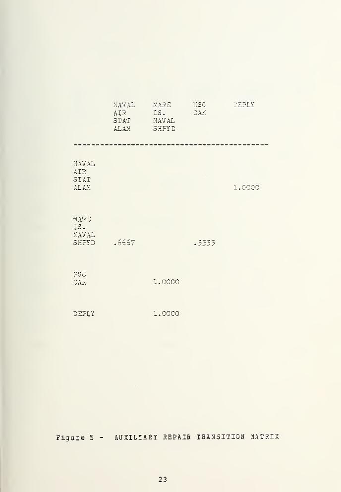
Figures 2, 3, 4, 5, and 6 show the matrices for each
ship class. They were developed by first identifying the
ports visited by each ship class. Those ports were then
annotated on the left vertical and top horizontal sides of
the class matrix. Next, these vessels' movements (Figure 1)
were annotated in the matrix as follows: a. The initial
location of a vessel was identified on the left vertical
side of the matrix; b. The location that this vessel next
moved to was then noted it the top horizontal side of the
matrix; c. A check mark was then entered within the matrix
based on these two locations. This procedure was then
repeated using this ship's new location as the left vertical
starting port of the matrix. When all the vessel movements
within a class had been processed, the probabilities of
movement from one location to another were determined across
each row of the matrix by dividing all elements' values (sum
of a group of check marks) in a row by the total row sum.
If one were interested in determining the
probabilities where a AF3 would be expected to move given it
is at Alameda, Figure 4 would be utilized. Starting with
14

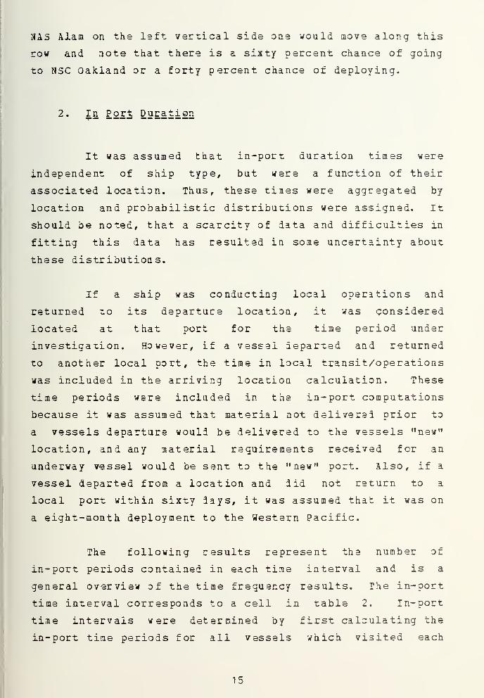
HAS Alam on the left vertical side one would move along this
row and note that there is a sixty percent chance of going
to NSC Oakland or a forty percent chance of deploying.
2 • Ib Por^ Duration
It was assumed that in-port duration times were
Independent of ship type, but were a function of their
associated location. Thus, these times were aggregated by
location and probabilistic distributions were assigned. It
should be noted, that a scarcity of data and difficulties in
fitting this data has resulted in some uncertainty about
these distributions.
If a ship was conducting local operations and
returned to its departure location, it was considered
located at that port for the time period under
investigarion. However, if a vessel departed and returned
to another local port, the time in local transit/operations
was included in the arriving location calculation. These
time periods were included in the in-port computations
because it was assumed that material not deliverei prior to
a vessels departure would be delivered to the vessels "new"
location, and any material requirements received for an
underway vessel would be sent to the "new" port. Also, if a
vessel departed from a location and did not return to a
local port within sixty days, it was assumed that it was on
a eight-month deployment to the Western Pacific.
The following results represent the number of
in-port periods contained in each time interval and is a
general overview of the time frequency results. The in-port
time interval corresponds to a cell in table 2. In-port
time intervals were determined by first calculating the
in-port time periods for all vessels which visited each
15


port. These periods ware then sorted by port. Time
interval (ceils) were next selected which would result in
approximately five in-port duration observations per cell.
Due to the extreme spread of the data it was not possible to
display the complete cell data for all ports. In some cases
so few data points were available that the above procedure
could not be done, and these cases were ommitad from the
Table. In other cases extreme values were observed which
were more than double the next largest value. These values
were in general considered outliers and were truncated from
the data set.
For example, the in-port durations for N&S Alameda
were calculated utilizing Figure 1. They were then ordered
and analyzed. The data was segmented into two groups.
Table 2 shows the first three ceils of this segmentation.
In this case, each cell represents four days. The remainder
of the distribution was also observed to be uniform (no
significent upward or downward trends) and they ranged from
twenty-seven to one-hundred and twenty-nine days.
Table No.. 2_j_ I N-
P
ORT gRBQOSNCY DATA
PORT
ALAMEDA
MARE IS
OAKLAND
CONCORD
TREASURE IS
DEPLOYED
ELL 1
5
6
6
7
6
9
CELL 2
5
5
4
5
7
CELL 3
5
5
2
5
These results are presented as a partial explanation
of the subjective determination of the in-port time
distributions. Upon completion of the inter-departure time
analysis, probabilistic distributions were assigned by
16


geographic location as follows:
a. Naval Station Alameda: The in-port time is
uniformly distributed between four and seventeen days with
probability 0.5, and uniformly distributed between
twenty-seven and one hundred twenty-nine days with
probability .5.
b. Naval Weapons Station Concord: The in-port time
was found to be exponentially distributed with the parameter
egual to .06 12.
c. NSC Oakland: The distribution was found to be
uniform between nine and fifty-six days.
d. Naval Station Treasure Island: The in-port time
is uniformly distributed between three and seventy-eight
days.
e. San Francisco Shipyard: The maintenance time was
seven days with a .65 probability, or was two-hundred-forty
days with a .35 probability.
f . Todd Shipyard (Alameda) : The time distribution
was found to be uniform from thirty-eight to eighty-four
days.
g. Bethlehem Steel Shipyard (San Francisco) :
Maintenance periods were either thirty or one-hundred-eighty
days with egual probability.
h. Triple A Shipyard (San Francisco) : In-port
time was found to be seven days.
i. Merritt and Pacific Shipyards (Oakland) :
Maintenance time was forty-four days for both locations.
17


j. Mare Island Naval Shipyard: The maintenance
periods were uniformly distributed between three and
twenty-eight days with probability .668 or uniformally
distributed between forty-three and ninety-one lays with a
.332 probability.
k. Deployed: The time in this catagory was assumed
to be uniformly distributed between fifteen and sixty days
with probability .65, and was two hundred and forty days
(eight-month deployment to the Western Pacific) with
probability .35.
18


ec<
L
tn
8^u to2 C< Lkj
K * Oa"- K 25 < =< 2 > ^ 2— in — ^ _= > C^» . K <Q cj -Ccr < c
UJ Ji < ^u; a_ _ v o
2 < s ls 5
Lu £T < UJ < UJ
rs. « tj, 2 = 2
a: u<
= g
< 2 <— —
23 <- ,w OZ 2
; wj
k >< <2 2
£252" O >- 2 a.
5 —> 2 £a < c
WS3owoCO
dcow>
0)
•Hfa
— m fn t in o
12 CD C* < < 5 £ < 2 S < «S"', <'5r0|N= N 2 N ^5flO N^^§ 2ll.- a: | mZ „On x OjOu
£ £ £
19


ICZ2h- >< <LL c o^ cr
hi J-
:--o
^ _i 1— 2C
,-M
oa
o
in
3
rn ar* \r\
—
4
"j
r>- o_Jl/>V— <_J ("VI o<a<-£ r*. oX.H-Q rvj '"J*
«^ U. <y")(_J • •
iC3
~C•_ i-JO NciCvno r\<i—>C <r
oo
lTi o
!35o
m m.* f\J
• •
r\ a ao ">» -^ "3
"3 ^ f! ~3
a -- \i O-4 • • •
HOS
oMMCO203e-t
zO
OS
—
MX
u
cn•Hf-bi
< _i r— i ^.'jO'-c>- -i2.<-zz ^ <; <i < :> ui >
'
X<Tt— —J i. -i <^ —j'-O'-J U_ _ l—"Z. r><. Z. in z. -« </) </i
r_j-d^
. v) J£ L_
20


NAVAL NSC 3ETHAIR OAK SHPYDSTAT SANALAM FRAN
DSPLY
NAVALAIRSTATalam .3333 oo / .5000
ns;
5000 .5000
TODDSHPYDSANFRAN 1 .0000
BETHSHPYDCJ A WJ n.+ <
FRAN 1 .0000
DEPLY 1 .0000
Figure 3 - AUXILIARY REPLENISHMENT TRANSITION MATRIX
21


NAVAL NSC TODDAIP OAK SHPYDSTAT SANALAM FRAN
NAVALAIRSTATALAM .6000
NSCOAK .6000 .2000
TODDSHPYDSANFt?AN 1.0000
TRPL ASHPYDSANFRAN 1.0000
DEPLY
./fOOO
.2000
DEPLY .5000 .5000
Figure 4 - AUXILIARY REFRIGERATED STORES MATRIX
22

NAVAL MAP E NSCAia IS. OAKSTAT NAVALALAM 5HPYD
DEPLY
NAVALAIRSTATALAM 1.0000
MARSIS.NAVALSHPYE f r /- rnno/CO! .3333
NSCOAK I. OOOO
DEPLY 1.0000
Figure 5 - AUXILIARY REPAIR TRANSITION MATRIX
23


NAVAL SAN T.I. MERRITT PACIFICAIR FRAN NAVAL SHPYD DRY DOCSTAT SHPYD SUP OAK OAKALAK ACT
DSPLY
NAVALAIPSTATALAM
SANFRANSHPYD
TODDSHPYDSANFRAN
T.I.NAVALSUPACT
MERR ITTSHPYDOAK
PACIFICDRY DOCOAK
DEPLY
.5000
1.0000
.5000
1.0000
.2222 .kkk5 .1111 .2222
1.0000
1.0000
1.0000
Figure 6 - MINE SSEEPER OCEAN TRANSITION MATRIX
24


B. MATERIAL REQUIREMENTS AND PROCESSING
The material requirements and distribution processes
experienced by NSC Oakland were reduced to a series of
inter-related functions. The criteria for this breakdown
was twofold: first, the function must be estimatable; and
second, only realistic processes were considered.
Suosequent paragraphs discuss the various assumptions
and procedures undertaken to quantify the inter-linking
segments of the material pipeline under investigation.
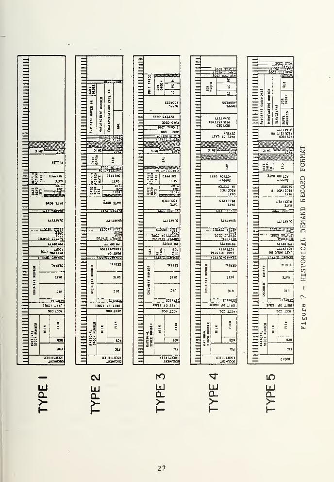
1 • Si§.^2£i2^i. Pep an d File
Numerous mechanized data bases were available at NSC
Oakland. However, after a detailed evaluation, it was
decided that the Requisition Demand History File (RDHF)
would provide the most useful data. The Requisition Demand
History File is a readily available mechanized file
encompassing transactions from two fiscal years. Figure 7
depicts the standard format of the file's five possible
one-hundred character records. These records will be
discussed below. This file is composed of those material
actions (requisitions) which have been transferred from the
Requisition Status File because of their historical
significance. Both the Requisition Status File and the
Requisition Demand History File are composed of records.
The initial basic entry which estaolishes the record is a
requisition and other pertinent data is subsequently added.
A record- by-recocd scanning of the Requisition
Status File is conducted to determine which records should
25

be retained because of their historical value. The
following decision parameters represent the significant
catagories of records which are transferred to the RDHF[ 11 ]:
a. Requisitions issued with and without proof of
shipment as follows: (1) if the record has been in the file
sixty or more days, without proof of shipment, a Record Type
four is assigned; (2) if the record has been in the file
sixty or more days with proof of delivery and the issue
group is one or two, a Record Type one is assigned; (3) if
the record has been in the file thirty days or nore with a
proof of shipment and the issue group is three, a Record
Type one is assigned.
b. Those records with an exception supply status
(rejected/canceled) as follows: (1) requisitions in the
"file for sixty or more days and and in issue group one or
two are assigned Type Code five; (2) requisitions in the
file for thirty or more days and in issue group three are
assigned a Type Cede five.
c. Records which indicate the item was sent to
purchase as follows: (1) if the record has been in the file
ninety or more days without purchase order data and is in
issue group one or two, or if the record has been in the
file thirty days or more without purchase order data and is
in issue group three, a Type Code three is assigned; (2) if
the record has been in the file sixty days or more with
purchase order data and the associated issue group is one or
two or if the record has been in the file for thirty days or
more and the issue group is three, a Type Cods of two is
assigned
.
26

cj4«i«
3lrO
bo gag.uurrno
DaeV;ams *34j4ig
-
<at. MIJJKMrag <u»«ar
33IA41SSrtSSI II in
oidiioaiuswooo
4UCD JIOH
5§ «u5
*at
ft
Si .
g* °
* 5mm S ! c
S S £
S i2e !»
jnimjl, !-:,,
aggjgJS^SfeiiS
aca
oo u3033 «0|ip»iisiLmiJlM
_,=>„ :3<jihs
|C 2 ! 3J.rO
1 J«Uss-
STr2-E I,il81ti
0A3« 11 ro
J4JU. Si Cv.'J
JU.ii.wno
813011 3H?5Tjo6mj21j
sruris a* *«*rtf
UIDOIU•oiirtirrsw
jo m04rijjns;n«vwa
M "l»l«3S
3* UMs
i i
8J
»W
la'] MiS30SSI iO 11 in
900 100*
£
S5» o 131
3SJ
aauiioailGMnooa
-£
ss3aoo»u.ns
1003 BgTj
Hnirmawra
33S aaaa
juiiwne
8BBB 8853
313303 RTOoSn
uiaoidd
aanaaBBB-I 33
trian
ZjEPQE3nssi io ii in
903 133Y
-IO J«t
— o- O
43 I J 11*301itttuooa
ZZ3
JlflBU. j^tD
30,03
^ ©«-»©
S5
u
IS34CKJY14405
JUIiWiTOouisinoM
03SIA34
SlUriS•isin jo lira
JIMIlliPI
slli?Mwa
Jira loijjr
tOiSJS 11
0JAI3334UN
03A 1331*3J.r0
iJil dHfl-TS
uiurno
".lllrli WI/BU
;c<fa
3003 siurls
Ul«0ld4
UiAiicrKI010M iST"l
tflJJnS/awHIa-
^
|
X
1a
T»(diS
3-tfQ
oin
iDiwns3IKSI iO um
900 U0T
-J 3
O »— u*- oK «9
X
:
13K
0SJ
« Hi 1*301lGMnOOO
jflfla nflrl
?rw
ai Is> *
i
»
^
3J.ro »oijjri"i«ns
lOJiiiI 03AI333JJ
uro
03AI3338liro
^^ 3i>flJ73
UllMflO
nun mriraauiiL
iiuusrshioiom isri
xiuns aurTBo"
Z 5
Z S
iria3S
JJIAajl
— 3ISSI JO iiM
Eh
aoEn
QgoWaQ
oMo£-•
COi-i
•H
LlI
a. a.>-
ro
a.UJa.
27


2. Data Base Establishment
Eight standard labeled IBM tapes were obtained from
NSC Oakland. These tapes were generated from the RDHF and
they contained all material transactions from September 1,
1976 to August 30, 1977. Over two million records were on
these tapes. The transactions encompassed local material
issues, demands for material not stocked at NS3 Oakland,
inter-depot transfers of material, and local procurements.
The customers creating the majority of these demands for
material were located worli wide and numbered oyer eight
thousand.
As only data for local customers was desired,
numerous extraction programs were developed. The resulting
data base contained only issues from stock for local
customers, including local procurements. Much of the
purification (duplicate records were discovered) and
extraction of this data was conducted with the assistance of
N. B. Nelson, LCDR, SC, QSN, a fellow student at the Naval
Postgraduate School. Upon completion of this reduction
approximately 600,000 records (four tapes) remained and it
was from this base that the vessel data was developed.
3 . Data Extraction
Those data elements actually extracted for further
analysis were common to all file records and in the same
data fields. Specifically, the data fields used were as
follows: a. the document number's unit identification code
(UIC) and date; b. the date received; c. the supply
action date; e. the quantity; and f. the priority.
23


The Appendix B program, AMG$DATA, extracted those
records from the local customer transactions data base which
met the following conditions:
a. Only those records of the previously identified
mobile customers were considered.
b. Of the above records, only those records which
the supply status code indicated that material had been
locally issued were actually extracted (supply status code
BA) .
Each data record which meet the above criteria, was
also coded to facilitate the identity of its owner and the
owner's ship class.
4 . Sample Size
In most cases the entire data base was used in the
determination of the simulation parameters. The quantity,
submission time, and process time parameters (as described
later in this chapter) were the only varibles in which a
sample was intentionally taken. This action was due to the
limited memory space available for the execution of the
FORTRAN program ANG$Dat1 and to keep the requirements down
to reasonable values so that the required data runs could be
made. In another case (Issue Group One priorities) a
smaller sample size resulted because its occurrance was very
scarce.
Tchebychef f s Theorem of Inequality [12] was
utilized to determine sample size because normality could
not be assumed to describe the underlying population.
Since it was desired that the sample mean would be
29


within one fifth of a stindard deviation of the true mean
with a probability of at least 0.95, a sample size of 500
was selected whenever possible.
5 • Data Reduction
The FORTRAN program which begins the data analysis
required for th9 simulation model is ANG$DAT1, Appendix C.
Numerous data arrays were developed for further analysis, as
follows:
a. Total daily requisitions submitted by each
customer were represented by a matrix (365x17) . The 365
dimension is the day Df the year the requisition was
prepared, and the 17 dimension represents tha seventeen
vessels under consideration. Quantities within the matrix
were the actual number of requisitions prepared on a
specific day by a particular vessel (we will call this a
requisition bundle) . Date differences for a giv=n customer
within this matrix will be called the "inter-preparation
times" for the bundles shown.
b. From the quantity field of the first 500
requisitions per local customer another matrix (500x17) was
developed. This was done because the data base was random
by customer and the quantity was assumed to be independent
of the ship's location and time. The 500 dimension in this
data array corresponds to the size of the sample, and the
seventeen dimension again represented those vessels under
consideration. The actual data elements in the matrix were
the quantities ordered pec requisition.
c. Submission time data for bundles of requisitions
was also considered independent of the vessel or its class,
and thus only one sample of 500 inter-arrival times was
30

extracted by selecting every one-hundred and eightieth
requisition. Its value was computed by subtracting the
document's date of preparation from the data of the
document's receipt. This action was considered appropriate
since groups of reguisitions were modeled, and it was
assumed all reguisitions ready for submission would be
submitted together.
d. The process time for a reguisition was modeled
as being dependent on the Issue Group of the reguisition.
This parameter was computed by subtracting the document's
receipt date from the document's ready for shipment date,
and was arranged into a matrix (500x3) . The 533 dimension
was the sample size, and the three dimension represents the
Issue Group. Individual data elements corresponded to
process times per reguisition priority by NSC Oakland.
6 . Bundle Preparation Time
Appendix D, ANGSFHIS, is the FORTRAN program which
differenced tthe document number dat.es as recorded in the
inter-preparation time matrix and utilized tha standard
library routine HISTG to produce a listing of the relative
frequencies of times' from one to nine days for each
customer
.
Analysis of this data revealed a significant
similarity of the output by vessel class. Figures 8 and 9,
and Table 3 illustrate this similarity. Note the small
values for the standard deviations of tha relative
freguencies at the bottom of Table 3. Because the relative
freguencies were so alike, the vessels were grouped by class
in this and all other vessel dependent parameter
evaluations.
31


Table NOj_ 3_._ RELATIVE FREQUENCIES OF INTER-PREPARATION
TIME
AE 1
TIMES BETWEEN BUNDLE PREPARATIONS IN DAYS
22 .51 .19 .14 .08 .06 .02
24 .54 .15 .11 .09 .04 .02 .01 .02 .02
25 .42 .20 .10 .10 .05 .04 .05 .02 .02
26 .53 .18 .09 .09 .06 .00 .03 .02 .01
29 .53 .20 .11 .08 .03 .03 .00 .01 .01
32 .56 .13 .14 .07 .04 .02 .01 .01
33 .46 .19 .03 .08 .08 .06 .02 .01 .02
35 .53 .16 .11 .10 .06 .02 .01 .00 .01
AVE .516 .175 .112 .085 .053 .024 .014 .011 .002
SI.DE .046 .026 .021 .010 .016 .013 .016 .008 .003
32


:c UU t f C I c S
o ^Z Z + 13 li- + + -I- + +-
10000000.5 J
tj
.'+0
. i;
.3.
J
• 25
,2 J
.15
.10
.05
s.-x x:
Mi
v
MMMMV,
.-.; :.: .: 1
!*? ;/,
M:.. -; -; -.* x V:x ,•; :.-.
, * -•• My.. x: -x
.'"' '' M
V.'.-i, * W M
rr ' -.(re J;
i*'
r,. fc i-., 'x i y~
i-. i ;:; . •>» - ,V, x
^c ate ^i>
*'• "• '/s-.
5X ~ #." " jW»*
: : „s
:
,' - rl 3?
A ;x -c ^c x M-*
r:^ 3»
"^ ^ (i ^£ :,; # , * ~ M*Ax.i o.
y--x
.r. : ; - X,
;;-- x M *- .'a -: * X M*W ".: * 1
s ' v ^::.;:* = i: i M £r.: x: ^ r
( ,* --* + M-x •x +
x ;; : : :-
.x -'x ;,: ^ v
O J 4, j; o • vj G d • .; 3 10.00 1 2 • J J
t
1 <+ .
Figure 3 - AS 22 BUNDLE INTEH-PRSP AR ATIQN HISTOGRAM
33


EOUtNCI tS
LOJ 2 4 25 1 2* + + + +•-
J j> + -+. +
J )
.3 J
tj
% J
3 3
30
,25
15
1 J
,05
7£lfi.iit M
$* -.<(
MS* 3p «« ,
'•'
** * * , M•;--^ & , -1
sic ^c 3St M
m -)» ;« vc
Vi .
-<¥ V , M-,':;t s- , Mf-f '
,'V|
a
-~ ~ , fa .
is;,-, rt(
V .
« '(i -£ , M*^s x
t •
.xr-. -.( M
M*— - , r£ ~ # , M_: :x s;
<jVi
#
"<=r « , y* ** -r , M 1
^ V -l- 4(
SssSSA( M
X- *i vi( M
r: v ^ t MH Sj! JS
( M .
M* .:; - _ .
; xi x Mrt ^ ,;
f ,
~v- ? , .
.; i! .<( M
.,: — -•: y. #
J-::*" , M5"^- =i , '.i .
:w
... ;.
""<•
'.' « .
:
Sf .£ -t •r r- M - - .
i< # -c(# is M as .-s
#~
' ^ - » ,>~ M i"
~^:.
t- ,c x:<
St T» M ; * .:--.:—
(
t» -,-.'•I
s1 = .
V i « *** ss ,M *-"-'.
:• ',' ' ,>* T* k'? :: .
* * :? , , ¥ £ M * .= .
¥ * :
:
>* s: ,v- s .
xx £ i:( ,
-»~ a :v' -s a
~ * :-.
> * -: .1.-: .:
***». , * « + ,v as Jc + .
u 21
. JO
:- + r; .; ; + ;- if ^ + - 3S * + B
I I "I+
t~ "I ~!c . i 10.00 i 2 . J w 14.00
Figure 9 - AE 32 BOtfDLE INTER-PHEPAfiATIOM HISTOGRAM
34

Upon completion of the class pooling of the data
several probabilistic distributions were examined for
applicability. Since the histograms were exponentially
shaped this was the first distribution tested. The inverse
of the mean value was used as the exponential parameter.
However, this hypothesis failed the Chi-square goodness of
fit test at the five per cent level.
Next an attempt was made to fit a geometric
distribution to the data. Inter-preparation times were
measured in the data base by one day increments. Therefore,
geometric parameters were established by assuming that if a
bundle was prepared within one day, there were zero days in
which a bundle was not prepared. We will denote P as the
probability of a bundle being prepared in one day. However,
if an actual bundle required two days to prepare, then we
will assume that there was one day in which a failure
occurred, i.e. no bundle preparation, and then a success.
If a bundle required three days to prepare, we will assume
there were two failures, i. e. day one and day two with no
bundle preparations, and then a success; and so on. This
results in a classical distribution with the following
probability mass function:
xf(X) = P(1-P) for x = 0,1,2,...
where,
x = the number of "failures" prior to a success
P = the probability of a success
Unfortunately this distribution also failed to fit
the data, although, it did provide a better chi-square
statistic -han did the exponential distribution.
35


A combination of two distributions was attempted
next. The author considered this approach because there was
a strong possibility that any single distribution would be
overwhelmed by the intar-preparations of one day. The
hypothetical probabilistic distribution was constructed as
follows:
1. Inter^preparation data of one day was separately
modeled. Therefore, the probability of a bundle preparation
occurring within one day was equal to "P ".
2. The remaining data was assumed to ba geometric
and the probability of preparing a bundle in two lays, "P "
,
was computed from the remainder of the data.
Tha detailed derivation of the above distribution
follows;
f(X) ={
P for x =i
C? (1-P) x = 1,2,...,2 2
where,
P = probability of a bundle preparation during
the first day
P = probability of a bundle preparation in two days2
f (X) = probability density function
x = number of days with no bundle preparations
36


General solution for C:
Q Xp + 2Z_ cp (1 - p ) =1
1 X = 1 2 2
nCP (1 - P l
^~ (1 - P ) = 1 - P2 2 x = 2 I
n x^ (1 - p i = 1/P if 0< (1 - P ) <1X = 2 2 2
:herefore
C = (1 - P ) /(1 - P ) .
1 2
The Chi-square statistic at the five per cent level of
significance and with nine degrees of freedom is 16.92. One
would accept this hypothesis if the computed statistic is
less than or equal to 16.92. The computed statistics for AE
class, AFS class, AOR class, MSO class, and AR class vessels
were respectively 7.544, 10.917, 19.419, 11.450, and 38.57.
The hypothesis that the distribution fits the data is
acceptable in three of the five classes. The AR class,
which had the largest error, was also the smallest in sample
size ( only one ship was in the sample ) . There were three
vessels in the other group which did not pass, however the
smallest value was generated by the largest sampla.
It is concluded that this developed distribution was
an acceptable simulation tool for the determination of
bundle inter-preparation times. The variable names
AE. 1UNDLE. INTER. ARRIVAL, AFS. 1 UNDLE. INTER . ARRIVAL,
AOR. 1UNDLS. INTER. ARRIVAL, MSO. 1 UNDLE . INTER . ARRI7AL , and
AF. 1UNDLE. INTER. ARRIVAL apply in the simulation.
7 • Mail Tia e pe r Bundle
The inter- arrival time distribution for bundles sent
by local vessels to NSC Oakland was modeled as being
37


influenced only by the 05 Postal Service and as such was
independent of both the vessel class and the material
requirements.
This distributiDn was tested using the Chi-Square
goodness of fit test and was found to be exponential with a
mean of 3*. 836 lays at both the five per cent and the one
percent levels of signif icance. It was assigned the
variable name MAIL. TIME in the simulation.
8 . Number of Re quis itions p er Bundle,
All the following distributions developed and
implimented in the simulation are empirical, except as
noted.
Five empirical distributions, one for each class,
were developed , from the data to describe the number of
requisitions per bundle. The following table lists the
probabilities of falling in the ranges shown based on those
distributions by ship class:
38


Table No^ 4._ PROBABILITIES OF REQUISITIONS pgR BUNDLE
Class Number of Requisitions
0-10 11-20 21-30 31-40 41-50 51-60 61-70 71-
AE .541 .172 .078 .062 .030 .035 .025 .029
AFS .692 .126 .036 .032 .019 .012 .003 .024
AOR .478 .162 .108 .075 .058 .038 .020 .041
AR .170 .091 .125 .095 .098 .106 .071 .124
Number of Requisitions
0-5 6-10 11-15 16-20 21-25 26-30 31-35 36-
MSO .591 .203 .076 .025 .017 .030 .000 .034
Although ranges were used in the above table, all
values utilized in the simulation were converted to
integers. These parameters were modeled as random linear
empirical distributions in the simulation. Their
identification is AS •REQ«PER«BUNDLE, AFS*REQ«PER •BUNDLE,
AOR«REQ»PER«BUNDLE, AR* REQ« PE R» 3U NDLE, and
MSO*REQ«PER«BUNDLE respectively.
9« Requ isitio n Priority
A probability distribution for material priorities
was determined by calculating the percent of requisitions
which were in Issue Group One (priority one through three)
,
the percent which were in Issue Group Two (priority four
through eight), and the percent which were in Issue Group
39


Three ( priority nine through fifteen) . It should be noted
that the requisition priority was considered independent of
both the individual ship and the ship class. Thus, only one
distribution was developed for all vessels. This approach
can be considered appropriate since all of these particular
vessels operate under the same priority determination
criteria. It was developed from the data as follows:
The issue Group One, requisitions of priorities 1
through 3, were tabulated and only 72 out of 94,434 cases
occurred. It was therefore very unlikely that an Issue
Group One event would be observed. In fact, this event
would be realized only .33 of one per cent of the time.
Issue 3roup Two, priorities 4 through 8,
requisitions were found to be more prevalent, being 14,157,
and their probability of occurrence was computed to be
.1499.
Issue Sroup Three, priorities 9 through 15, had the
highest observed incidence with a probability of .8493.
The simulation variable for this parameter is
REQ«PRIORITY.
10. Process Times_
The requisition process time was modeled as being
dependent on only th= priority (Issue Group) of the
requisition. This approach was considered reasonable
because different Issue Groups are actually processed
differently. The various picking documents for the material
are expedited to the warehouse and are colored differently
for high priority material (Issue Group One and Two).
40

The following distributions were developed by
subtracting the date of document receipt at NSC Oakland from
the date that the material was ready for shipment in the
data base.
The Issue GrDup One requisition process time
cumulative distribution was determined to be between 0.0 and
1.95 with probability .394, between 1.96 and 7.77 days with
probability .423, and between 7.8 and 29 days with
probability .183. It should be further noted that the
number of usable data points was less than 72 for the
following reasons; (1) the original number of data points in
this Issue Group was only 72, (2) entries in the data base
were discovered which showed that certain requisitions had
been shipped prior to receipt of the requisition, (3) other
date errors occurred; for example, several requisitions
showed that over 300 days were used in the processing time.
These types of errors also occurred in the other Issue Group
data bases and were also ignored in the distribution
computations.
The Issue Group Two process time cumulative
distribution was also between zero and 1.2 days with
probability .5, between 1.3 and 14.3 days with probability
.42, and between 14.4 and 38 days with a .08 probability.
The process time for Issue Group Three requisitions
was between zero and 1.2 days with probability .56, between
1.2 and 15.5 days with probability .395, and between 15.5
and 38 days with probability .045.
11. £uantitv p_er Re_ g_i is it ion
Since requisitions for material may be a request for
more than one of an item , the appropriate field in the data
41


base was utilized to evaluate the process. It was assumed
that the various quantities ordered per reguistion would be
dependent on the vessel class. Thus, five cumulative
distributions were developed.
Those quantities expected for an AE class vessel
were found to be between one and five with probability .608,
between six and ten with probability .238, and between 11
and 160 with a .154 probability.
The other vessel class distributions were modeled
with the same uniform ranges but differing probabilities.
In the AFS class, the probabilities are .576, .171, and
.253 respectively. The probabilities for the AOR class are
.612, .161, and .227; for the MSO class .559, .143, and
.298; and, for the AR class .496, .164, and .340
respecti vely
.
12. Weight p_er Requis ition
That data required for the parameter determination
of this attribute was not available. However the author
assumed. a classical exponential distribution with an
expected value of two pounds per each item. The mean weight
per requisition generated by this simulation was 193 pounds.
Hernandez and Gallitz [3] stated that 28,586,168 pounds
(fiscal year 1975), and 26,805,662 pounds (fiscal year 1976)
of material were delivered by the BALD system. This equates
to an average of 73 pounds per reguistion and 69 pounds per
reguisition respectively (assuming that there was not a
significent change in the total number of requisitions per
year from 1978) . Observitions by this author at the BALD
shipping and delivery points revealed that it was uncommon
to witness a full truck load shipped. In fact most
shipments were only one pallet level high, yet statistically
42


full truckload weights were recorded on the shipment
records. Because of this, it was suspected that the weights
[12] are overstated.
It is therefore concluded that the parameter of two
pounds chosen for the m=an of the distribution was too
large. Thus, the actual number of shipments made was
selected at a proxy measure of effectiveness for this
variable. Resultant outputs from this assumption have not
been included in the results section of this thesis.
43


III. SIMULATION
A. GENERAL
SIMSCRIPT II. 5 is a language particularly suited to
discrete-event step simulations. It has been designed to
facilitate the simulation of large complex systems with a
minimum of effort in programming, designing, and testing the
model.
It is not the intent of this paper to discuss the
details of this unique programming language, and anyone
desiring to examine it in depth should refer to raferences 9
and 13 .
3. PROGRAM DESCRIPTION
The modeling of that segment of the BALD system impacted
by the random movement of vessels between various ports was
developed by considering two major series of events.
First, the vessel movements were modeled using the
previously discussed parameters and techniques. This series
of events deals primarily with vessel movement impacts on
the ultimate destination of shipped material. This series
also rsmoves material from a "old" shipping queue and
relocates the material in the appropriate "new" shipping
queue corresponding to the vessel's nsw location.
HH

The remaining series of events recreates the material
processing involved. Their logical functional order
commences with the preparation of a group of material
reguirements. Next, this group of material reguirements
arrives at NSC Oakland and is reduced to its individual
material reguests. These requisitions then are scheduled
through the material processing system and a shipment
availability time is determined. The final events collect
statistics and determine the freguency and the destination
of the various shipments.
1 . Detailed Analy si s
The preamble defines various system variables,
events, and entities. Actual execution commences with the
main program. It first assigns user defined values to the
permanent entities (ships). This segment then reads all the
program decision variable distributions, schedules an
initial port change and bundle preparation for each vessel,
schedules the initial shipments to each port, and schedules
the two one-time events, 3 top. simulation and Equilibrium.
From this tine on the SIMSCRIPT event step
simulation time scheduling routine takes over. Events will
occur as determined by the scheduling parameters throughout
the program. The specific events are detailed below.
Bndle. preparation: This event schedules the next
bundle preparation for each vessel based on the -Lass of the
vessel. It then determines the the valie of the
number. of .requisitions (bundle) and then schedules an arrival
time at NSC Oakland-
Arrival, of .bundle: The temporary entities,
requisitions, are created in this event. They are assigned
45

all their attributes (priority, quantity, and customer)
based on the previously discussed parameters. Then a
Ready .for .shipment event is scheduled based on the
requisition's priority. Finally, the temporary entity
bundle is destroyad to release memory space in the computer.
Change. location: The vessel's new location is
determined based on ship class markov chains. Statistics
are accumulated to record both the number of location
changes per vessel and per vessel class. At this time, if
this vessel has any material in one of the poet shipping
queues, it is removed and put in the newly determined port
shipping queue. The system statistics are also
appropriately adjusted. Finally, the next port change for
this vessel is scheduled based on the vessels current
location.
Ready, for . shipmei t : The shipping location is first
determined, and the requisition is filed in the appropriate
shipping gueue. This event also may schedule an immediate
shipment of matarial depending on the decision rules
involved
.
Shipment. to: This event computes the majority of %
the statistics. It also contains all decision rules on
shipping stratagy. Upon completion of this event the next
shipment to is scheduled for this port.
2 . Seed
s
Since the pseudo random number generator was seed
dependent, ten seeds were initially selected and program
runs were made to identify equilibrium conditions and
reverify the simulation's validity. The seeds ware selected
at least BOO, 000 numbers apart to preclude overlapping of
46

the number stream.
In order to to evaluate the stability of the
measures of effectiveness as related to seed changes, Ten
runs (one run per seed) were made with each decision rule.
It was noted that in some instances the SIMSCRIPT program
exceeded the 430,000 bytes allocated . Since the variations
in the measures of effectiveness (average wait time and the
number of shipments) were minimal, it was not considered
necessary to rerun these programs, see Appendix H.
3- Equi li brium Determination
The equilibrium oc steady-state of the system is
defined as a condition of regularity of stability in which
opposing influences are balanced. Thus, it is assumed that
for this model there is a limiting probability distribution
of the responses that is charactertistic of the system.
This state was determined by a method stated by Conway[5].
Specifically, the series of measurements were truncated
until the first of the series was neither the maximum nor
the minimum of the remaining set.
The number of requisitions shipped to each port was
one of the measurements evaluated in the above manner. The
determining port was tf.A.S. Alameda and the time to
steady-state was two weeks. Inadvertently, the number of
shipment's variable was not adjusted for this two week
period and a lack of time precluded the rerunning of this
computer simulation. Thus, this measure of effectiveness
was accumulated over a fifty-four week interval.
A determination of the equilibrium condition for the
ship movements was not made. The initial starting
conditions for the simulation were chosen so that they were
47

typical of the steady-stite condition. For example, all
vessels were initially located at factual locations, rather
than positioning them arbitrarily and then determining the
steady-state condition.
**• Shipping Strategies
Four shipping flecision rules were analysed as
follows: a. CASE I - all material ready for shipment is
shipped daily; b. CASE II - all material ready for shipment
is shipped weekly; c. C&53 III - in addition to CASE II
actions. Issue Group 1 miterial (with all other destined for
the same location) is shipped immediately; d. CASE IV - in
addition to the CASE III decision rules, Issue Group 2
material (again with all other material in the appropriate
queue) is shipped once a day.
Appendices E, F, and G contain those events which
were modified for each daoision rule.
5. Measures of Effectiv en ess
Two measures of effectiveness were selected. First,
the amount of time requisitions were waiting to be shipped
was chosed as a measure of customer service. Second, the
actual number of shipments released was selected as an
evaluation of the cost of the chosen stratagy. The total
number of shipments is considered a proxy variable for
shipping costs.
C. RESULTS
48

The outputs from the forty -program runs have been
tabulated by each decision rule and are presented in
Appendix H. The logically expected results in the mean
waiting times was observed. Mean waiting times of .48 to
.53 were observed when shipments were daily. Under weekly
shipping rules the mean waiting times were 3.41 to 3.61
days.
Since program runs were seed dependent and a comparison
of decision rules was desired, only those runs in which all
results were obtained for all cases will be examined here.
These runs were numbers 2, 3, 5, 6, and 8 as found in
Appendix H. Data fron these runs were then averaged by
Issue Group within each decision rule (case) . Weighted
averages were then computed per case by assigning weights
which were representative of each Issue Group's probability
of occurrance. The values used were .0008 (Issue Group
One), .1499 (Issue Group Two), and, .8493 (Issue Group
Three) . The results of these computations represent five
years worth of simulation per case and are presented in
Table 5.
49


I able NDj. 5_. AVESAgED RESULTS
CASE
II
III
IV
ISSUE MEAN STD MAX MIN TOTAL
GROUP TIME DEV TIME TIME TRIPS
1 . 49 . 29 .99 .01
2 .50 .29 1.00 .00
3 . 50 .29 1.00 .00 2076
Ave . 50 . 29 1.00 .00
1 3. 48 1 .39 6.92 . 14
2 3. 52 2.01 7.00 ,00
3 3. 51 2.02 7.00 .00 319
Ave 3. 51 2.02 7.00 .00
1 . 00 .00 .00 .00
2 2.93 1 . 99 7.00 .00
3 2. 91 1. 99 7.00 .00 337
Ave 2.91 1 .99 7.00 .00
1 .00 .00 .00 .00
2 . 49 . 29 1.00 .00
3 . 52 .38 6.93 . 00 1353
Ave . 52 .37 6.04 .00
50

IV. DISCUSSION AND CONCLUSIONS
A. DISCUSSION
It is noteworthy that minor variations in the average
waiting times have significant impact in the total number of
shipments. Increasing the waiting time per shipment from .5
to 3.5 days has the effect of reducing the number of
shipments from an average of 2076 to an average of 319 trips
per fifty-four weeks. or a 6.6-fold decrease.
However, adjusting the weekly shipments by shipping
Issue Group One material immediately (CASS III) reduced
their waiting times to zero, yet did not significantly
increase the total number of shipments experienced. In
fact, they only increased from 3 19 to 387 per 54 weeks.
This is not an unexpected result since there was only a .08
per cent chance of a vessel generating an Issue Group One
shipping requirement.
Finally, CASE IV decision parameters resulted in almost
the same number of shipments as when daily shipments were
made. The average number observed for 54 weeks wis 18 53, on
the average only 263 shipments less per year.
The weighted averages of each case were used to
construct Figure 10. The dependent variable wis the mean
wait time in days and the independent variable was the
number of shipments made in fifty-four weeks. The curve was
constructed assuming that the unknown function was
51


"hyperbolically" shaped. This assumption was supported by
the observation that as the number of shipments approach
infinity the average waiting time would be expected to
become zero, and as the number of shipments approach zero
the average waiting tine would be expected to become
infinite
.
52


4- \
UJ
><oLd
X
UJ
5
\
\
\
ur N\\\\\\^\s
+ -4- -}-
NUMBER OF SHIPMENTS 2000
Figure 10 - SHIPMENTS VS WAITING TIME
53


The curve of Figure 10 provides a practical tool for a
decision maker. If an objective function is known (such as
a decision maker's relationship between the relative
importance of waiting times and the number of shipments) ,
the "optimum" number of shipments could be determined. For
example, if it was decided that the number of shipments was
twice as important as waiting times, an objective function
could be constructed as follows: total cost = (cost
constant) x (waiting tima) + (cost constant) x (2) x (number
of shipments) . The appropriate cost constants would have to
be selected to convert the variables to dollars. This
objective function could then be used with the curve to
determine an "optimal" solution. However, this solution
should not be attempted until additional simulations are run
to verify the midrange of the curve.
3. CONCLUSIONS
In view of the simulation results, it would appear that
actual modification of the current shipping parameters may
yield substantial transportation savings. However, because
such parameters as the weight and volume of the larger
shipments were not evaluated, delaying a shipment beyond the
time when a full truck load is ready for shipping would not
be expected to result in any savings.
It is recommended that follow-on modeling in this area
be conducted. The weight and volume parameters should be
identified and decision rules should be modified to include
maximum and or minimum weight/volume shipping restrictions.
Additional shipping strategies (cases) also need to be
proposed and analyzed (for example, allow Issue Group II's
to be shipped every other day, every third day, etc.) to
54


fill in the middle of the curve of Figure 10. Finally, the
simplifing assumptions of the model presented in this paper
need to be critically reviewed and any which seriously
violate reality should be replaced by more realistic ones
and the analysis repeated.
55


APPENDIX A
SHIPS INFORMATION BULLETIN
NAVSUPPACT-3Q SHIPS INFORMATION - 7LS-babl SUNRISE SUNSET0=100 UNIFORM PORT SERVICES OFFICE iaQS3GU iaia43U13-24 APR 73 NAVAL SUPPORT ACTIVITY n0S2=!U 11ia i!fiU
{TUE-MON* TREASURE ISLAND 20QSE3U S0164TUSAN FRANCISCO-. CALIFORNIA =14130 ElOSEbU S113S0U
AREA CODE 415 UNLESS OTHERWISE INDICATED E20S2SU 2E1351UE30SE4U 2313SEUE40SS2U S413S3U
SOPA SFRAN-, COMSERVGRU ONE-. CAPT E.J. MESSERE-. USNSOPA SUBAREA SOUTH-, COMSERVGRU ONE-, CAPT E-J. MESSERE-, USNSOPA SUBAREA NORTH-, COilSERVRON THREE-, CAPT C • Id • O'REILLY-, USN
COMCARGRU THREE - 3^=1-2131COMSCPAC - 4bL,-b31bCOMSERVGRU ONE - 4bb-5312
• COMSERVRON THREE - 70?-L,4fc.-3S3a
SHIPS PRESENT SAN FRANCISCO BAY AREA
SHIP HULL BERTH PHONEiLTfiD T-AK-277 NSC 4bL,-5 c!S0
BROSTROM T-AK-2S5 NSC v/ / 4tb-S710CARPENTER,. . DD-3S5 NAS-*^ /AV/7T- <*^ 8b=i-3037C0QK£rc y/?/?f FF-ioa3 triple a shpyd 3S2-2120EXCEL .. . MS0-43=i TODDS SHPYD ALAMEDA 523-0321FANNING BfZ. */iihf FF-107b TRIPLE A SHPYD a22-23b0FLINT ' AE-3E N A S - £r# */&V- ci/f^sr* flbi-37bbGALLANT £.rt,5filJ7t f1S0-43=l PACIFIC DRYDOCK a^3-!C^EHADDOCK ere **/'3-/7f SSN-bSl MINSY 707-b4b-4370HALEAKALA AE-ES UPNSTA b71-5004HECTOR AR-7 NAS 6^-3^70HEPBURN £rc+ y/^/7 fFF-1055 TRIPLE A SHPYD. _ 332-3711KANSAS CITY
'AOR-3 NAS - 5 /"^ %3 y/>f'J> ab=l-202Q
KISKA AE-3S NAS- Sro V39/?r- S*<r~ 3b=i-3b5aMAUNA KEA AE-22 TODDS SHPYD ALAMEDA S23-0321MOUNT HOOD AE-2T NAS 8b=i-4722MYER T-ARC-b NSC 4bb-5001PERMIT SSN-S=iS MINSY 707-b4b-32b4ROBERT E. LEE^r-f^A/SSBN-bQl MINSY ?07-b4b-3432SEAIdOLF / SSN-S7S MINSY 707-b4b-41 c
J7
SHASTA AE-33 TODDS SHPYD ALAMEDA 3bS-044STAUTOG SSN-b3=i MINSY 7Q7-b4b-4150VANGUARD T-AFM-l=i NSC 4bb-b3=iaUABAZH&rc Y'f/?? AOR-S TODDS SHPYD ALAMEDA 523-0321
56


APPENDIX B
FORTRAN PROGRAM ANG DATA//AN// E//FP
10100
20
22
24
26
23
30
32
34
36
GSDAXECRT .S
INDAOTREFQINIFINI«=
IUWRIF
.ICIFIUURIF
. ICIFIUWRIF
.ICIFIUWRTF
.ICIFIUWRIF
.ICIFIUWRIF
.ICIFIUWRIF
.ICIFIUWRIF
. ICIFIUWRIF
.ICIFIUwR
TA JFootYSINTEGFTA I
MENSA0(1RMATRl =(ICLR2 =
(IUICI =ITE((INPLJS(IUIIC =ITE((INR.LUS(IUIIC =ITE<( INRLUS(IUIIC =ITF(( INFLUS(IUIIC =
I T E(( INRLUS(IUIIC =
ITE<(INPLUS(IUIIC =
ITEI(INPLUS(IUIIC =ITE((INRLUS(IUIIC =ITF((INPLUS(IUIIC =ITE(
C8 (2427, 0331, RZCLG00 *
R*2 ISTAT fT3A
BA/*BA*/ 9 IN<U/0ION CATA1(10),QA0, 100, END = 999
)
CCA4,2A2, 1 244, I
INP1 + I
US .NE.10 .OR. I
INR 2 + 1
C .NE. 13) GO T
10120, lOOJOATAl,! S T
2.LE.1000)WRIT=(
C .NE. 29) GO m102
20, ICO) DATA! , 1ST2.LE.1000)Wo ITF(
C .NE. 37) GO T "
10320,100) DATA1 , I ST2.LE. lOOO)WRITc {
C .NE. 7 8) GO TO1C4
2Q,100nATAL , 1ST2.LE.1000) w* I
T E(
81) ,'EA T =2 740', T I^ C =75
/, INR2/0/TA2( 13)DATA1,ISTAT,D4T
3,T3 ,12)
STfiT .NE. IP A) G
20
*T f DATA2,IUIC, II30, 1C0)QA7A1, 1ST
22
AT,0ATA2 ,T'iir, t t
30, 100)OATA1,I ST
24
4T, DAT A?, IUIC, II30, 1C0)DATA1 ,ist
ATf 0ATA2, IUIC, I
T
30,100)CA TU ,IST
A2, IUIC, II, ICL I
J TO 10
,ICLUSAT, DATA 2, IU
, ICL'JSAT,PATA2,I
, ICL'JSAT,0ATA2 , IU
, ICLUSAT,0ATA2, IUIC,
I
C .NE. 25) GO TO 2810520, 100JCATA1, 1ST2.LE.1000)W»TTC(
C .NE. 24) GO T^106
20, ICO )0ATA1 , TST2.LE.1000)W= Itc
(
C .NE. 15) GO TO1C7
20, 100)0ATA1,T ST2.LE.1000)WRITE(
C .NE. 23) GO TO1 C8
20, 1CC)DATA1,TST2.LE.1000)WR I
T E(
C .NE. 9) GO to2C9
20, ICC )0ATA1 , I ST2.LE.10CO)W !
T r(
C .NE. 3) Gn TO210
2C,100)PAT£ 1 ,1 ST
AT, 0ATA2, IUIC, T
I
30, lOOHA^il ,1 ST
30
ACQATA2, IUIC, I
!
30,100)DATA' ,IST
32
AT, PATA2, I'1 T C , I I
30,100)0A T A1 , 1ST
34
AT, DATA 2, IUICI I
30, 100)DATA1, !
S
T
36
ST, AT A2, IUI CI I
30, lCO) n A T Al, T ST
39
, ICLUSA7,0ATA2 tllJ
, ICLUSAT,DATA2, I J
, I C L U SA T ,DATA?,IJ
, ICL'JSAT, DATA 2, T
)
,IC LUSAT, DATA 2, 1
J
IC I I
t r, I I
AT,qa t A2,I JIC, T I , ICLUS
57


IF(INR2.LE.1000)W?TT=(30, 100)0A X A1, T S^ AT , DAT 4 2 , ! J TC T'
. ICLUS38 IFdUIC .NE. 14) GO TQ 40
I'JIC = 211WR ITE< 20, 100) 0A T A1 ,1 S^C0 AT ^ 2 , I'JIC I I ,ICLUSIF( INR2.LE.1000)WR TT =(3C, ICO) DATA I, 1ST AT , DATA 2, IUIC ,1 T
.ICLUS40 IFdUIC .NE. 21) GG T 42
I'JIC = 312WRI T E( JClOCinA^ 1 ,1 S T AT, DAT 42, 1 Ml CI I , ICLUSIFdNR2.LE.1000)*°ITE(30,100)DAT41 t ISTAT,0AT4 2, T UTr t I T
•ICLUS42 IFUUIC .NE. 19) GO Tn 44
IUIC = 313WRITE< 2C,lC0)D4TACTSTaT,DATA2,rJ!C ! I ICLUSIF(INP2.LE.1000)U? I TEC 30, ICO) DATA 1,1 ST AT , DATA 2 , 1 J I C ,
!
T
.ICLUS44 IFdUIC .NE. 11) GO TO 46
IUIC = 314WRI TE( 20, 100) DATA 1,1
S
T AT ,DATA2, IUIC, II , ICLUSIFdNP2.LE.10G0)WRITP< 30 , 1 CO ) DA ta 1 t I ST AT , DATA 2 ,
T U Ir
,T T
.ICLUS46 IFdUIC .NE. 46) GC TG 4^
IUIC = 415WR IT E ( 20, 100) D4TA1 , I STAT, DAT A2, IUIC I I , ICLUSIFdNF 2.LE.1000) WQ I T=( 30,100)^.^1, 1ST AT,DATA2, I'JIC I I
.ICLUS48 IFdUIC .NE. 45) GG TO 50
IUIC = 416WRITE (20, 100)04TAldST4C0ATA?,THTC II , ICLUSIF(INR2.LE.1000)W5IT E (30,1 00) DATA"* , I ST AT , DAT A ? , I J I
r, tj
.ICLUS50 IFUUIC .NE. 5 J GO TQ 10
IUIC = 517W ITE( 20, 100 ) DATA 1, I ST at, qaTA 2, I U IC T I, I CLUS
IF(INF2.LE.1000)WRITE(30,100)OATA1, T S^ AT , DAT A 2 , IJ
I
r,
' T
. ICLUSGO TC 10
999 WRITE(6»200)INR1,INR2200 FORMAT ( IX, 'TOTAL RECORDS = ' , I 7, 10X ,
« TOTAL 8A RECORDS.= », 17)END FILE 2END FILE 30STOPEND
//G0.FT10F001 CC UN d = 3400- 3 ,VPL=SEF =^ D S 707, DI SP=
(
OLD,*E=P )
,
// LABEL = d,SL,,IN) , DSN = S2 3 90 .LOC. DLV . SORT ED .U I r .v//GO .FT20F0C1 DO DSN=S2427.L0C. SHI P. BA» V0L=SER=NPS7 15
,
// DISP = (OLCKEEP),// UNIT = 3400-3,LA3EL=d , SL, ,OUT) ,DC8 = ( RECFM = FB, LRECL = ?.30 , )
//,BLKSIZF=800C)//G0.FT30F0C1 CC DSN=S2427 .LOC .SHI P .BA, LABEL =EXPHT=79365,// SPACE = ( 20 CO, 155, 5) ) , VOLUME = S ER=OUF FY , D I 3 P = ( OLD, K EE D
) ,
//UNIT=2314
58

APPENDIX C
FORTRAN PROGRAM ANG DAT1
THEFORTHE//AN// E//FQ
10
100cc
cc
20
2122
1324
FOLLOWING PROGRAM EXTRAC T S tha t DATA NPCESS4 D YTHE DE TFRM INAT ION HP TH C matpptal PARAMPTFRS OPSIMULATION.GSCAT1 JOB (2427, 0331, PZ81) , 'EXT=2740' ,
T IV^ = 60XEC FOPTCLGRT.SYSIN DD *
REAL*S UICLCCDIMENSION NUMB (367,1 8) ,
T QUA'-!( 500 , 1 8 5 , MA T LT { 5 00 ) .
.»IGR0UP(4),UICLGC( 13) ,NN( 1 7) ,PGROUP( 4) ,MA PR I ( 500* 3
)
.IPROC(500,4)CATA NUMB /66 06*0/, TQU^N/90 00^0/ ,^ATL T / 50 0-0/,
., I GROUP/ 4*0/ ,IDP T /0/, II /O/, 12/0/, I 3/0/, 14/0/,'• K/0/,A/l .0/,NN/17*0/ , IFLGl/0/* IFLG2/0/ , M APR I / 1500*0/*. IPROC/20CC*C/CALL SETIMEREADd 0,1CC,E^0=', 6 ) IOi T Pi , IPRI ,IQN,T0ATE2, IDA T E3* T UTrIF { I PR I .EO. 0) GO ti ioIFdUIC .EC. 18)IJTr = 01IFIIPRT .FO. 1003WRITE (6,100) I t,TE 1 , I P° I , ION , I Oi T r-2 ,
.I0ATE3, IUICF0RMATC27X,I3,8X,I2,4X,I5,2X,I3,5X,I3,31X,I2 )
IFdDATEl .GT. iniTP 2 ) IV^EZ = IQATE2 + 3o5IFUDATE2 .GT. IDATc?) IDATE3 = I0ATE3 + 365NUMB. IDATE1, IUIC) = NUMB ( I DAT C 1* T'J IC ) + 1
IFUPR I .GT. 3) 00 n 20IGROUP (1 ) = I GROUP ( 1 ) + 111=11+1
IF(I1 .LE. 500) IPR0C(T1,1) = I^ T
IF (II .LE. 50 0) MAPRI(I1,1) = lOATP?IFdPPI .LT. 4 .OR. IP- 1 .GT. 8) OPIGROUP (2) = IGROUP (2) + 1
IFUFLGl .L T . 1 0) GO tp ?1IFLG1 = C
12 = 12 + 1
IF { I 2 .LE. 500) IPR0C(I2,2) = IOATIF (12 .LE. 5 00) MAPOl(T2,2) = I0ATE2IFLG1 = IFLG1 + 1
IF( IPR I .LT. 9) GO rn 2 4IGROUP (3) = IGR0UP(3) + 1
IF(IFLG2 .L T. 90) GO to 23
IFLG2 =13 = 13 + 1
IF(I3 .LE. 500) IPR0C(I3,3) =
I'M 13 .LE. 5 00) MAORI (13,3) = IQATE2IFLG2 = IFLG2 + 1
CONTINUENN (IUIC) = NN( IUIC ) + 1
K =NM IUTC)IF(K .LE. 500) IQ'JAN(K* IL'IC) =IQN
C0UNT1 = C0LN T 1 +1.0IF (COUNT 1/13 0.0 .M = . &) CO to io
A = A + 1
14 = FIX(A)
E3 —- 10
Tn 2 2
"5 —- I
I0AT r 2ATF*
IOAT=?ATE1
t c; _0A T E3- in
I0A T E2H:l
59


26
1111
IF ( A .LEGO TO 10CONTINUEigroup(I) = rCALL GETI^E( I^T)SECS = IET* C. 000026WRITE (6,1111) SrCSFORMAT (P16.12)IGR0UP(4) =IGR0UP(1)
500) MAIL T(
T 4) = I0ATE2 - IDiTEl
112
33
CC
115
C
122
120
124
130
34
132
131
134
135
136
150
153
156C
PGROUPt 1)PGROUP (2)PGRCUPO)DO 32 J=lDO 23 1=244,365IF (NUMB (I, J) .MPFORMAT (213,16)CONTINUECO 30 1=1IF (NUM8(CONTINUECONTINUEEND FILE
+ Tr,Rn'jp(7j + IGonUP{3)= FL0A T
{ I GROUP < 1) ) /FLOAT ( I GROUP (4) ) *U0= FL^AT( IGR0t)P(2) ) /FLOAT ( IGR0UP(4) )*1QC= FLOAT( I GROUP (3 ) ) /FLHAT< IORQUP (4) ) *} J J17
,243I, J )
0) WRITE (20, HO) I , J , NUMB ( I , J )
•NE. 0) WPTTE (20,110) I
,
J,NUMB( I ,J
)
20
PRINT MATRIX 9 COLUMNSPEAO(5,U5)UICLOCFORMAT (A6 )
JENO = 17NEND = JEfsO - 1
A TIM!
CO 34 NMEND =
WRITE(FORMAT { •
WRITE(6,FORMATdWRIT = (6,kRITE(6,WRITE( 6,FORMAT <
'
WRITE(6,WRITE( 6,FORMAT (I
. 16, 2X, 16CONTINUEWRI^E(21FORMAT (
WRI T E(6,FORMAT {/WRITE( 6,FORMAT (I
.I5, T 65,'WRITE(6,FORMAT (
•
.MAIL TIMREAD(5,1WRITE(6,FORMAT (2
WRITEFORMAT (1WRITE( 22WRITE(23FORMAT (
I
WRITE( 7,FORMAT (2
= 1,N +6,121', 1
120)IX. 9130)130)124)1M120)13C)6,2X,2X)
,13212,1131)///)134)OX, •
PERC135)1* ,1E'//15) (
136)OX,
3
(6,12X, I
, 132,1536)156)0(11
NEMO,
9
82)5X, 'FREQUENCY OF ? EON c BY SHI^*//)(UICLOC (N!) ,NI=N,NIEND)
( A6 V ?X)/)(MJ, (NUM8(MJ ,NK) ,NK=N,NIENO) ,NJ=244,365)(NJ, ( NUMo (MJ,,\K) ,NK=N,NIEMD) ,NJ = 1 ,243 )
5X, 'CUANT T-ry P C R REOM PY SHIP*//)(UICLOC(N T
) ,NI=N,NIEND)( N J , ( I Q U AM { N J , NK ) , N K=N , N I E NO ) , N J=l , 5 0),l6,2X,l6,2X,I6,2X,l6,2X,!6,2X,Io,2X, T o.2Y
) ( ( J, IQ!MN( T , J) ,T =i ,500) ,J=1 , 17 )
c)
( I , IGROUP( I ) ,PGR^'JD( I ) ,1=1,3)ISSUE GR n n^> ',11,* TO^AL NR O c REQ:*, T 56,ENT:«
,
?X,F5.2)
OX,«NSC I^SUE/SHlo TIME BY IGRP AND 3 EQM')
UICLOC ( I ) , T=l,4)(UICLOC( I },!=!, 4)
!( 46, 2X)
,
10X,A6).50) (I, MPROCC I,JJ,J=1,3) ,MAILT(! ) ,1=1,500)! 7, 16,2 X , 16 ,2X , 16 , ?X , 1 OX , 1 6 )
!)(( J,! OR DC (I, J ) , J = 1,3) ,1=1,500)i)CM4ILT(I ),I = 1 ,500)
UJfMAPRI (I, J),I = 1,500), J = 1,3)( (J,MiPPT ( T, J ) ,1 = 1, 500) , J =
,13))
CALL GETIME(I=T)SECS= IET * 0.000026
(6,1111) SFCSWR ITSSTOPCEBUGEND
//G0.FT10F001 CC
SUBCHK
DSN=S2427.LCC SHlP.8 /\tVnL = SE^=NPS71
60


// DISP// UNIT =//G0.FT2// DSN=S// DCB=(// OISP=//GC.FT2// DSN=S// DCB = (
// DISP=//GG.FT2// DSN=S// oce=(// DISP=//GQ.FT2// DSN = S// DCB = (
// OISP=//GO.SVS
1
2345678
AEAEAEAEAEAEAEAEAFSAFSAFSAORAQRAORMSDMSOAR 7DUMMYIGRP 1
IGRP 2IGRP 3MAIL
=(OLD,KEEP) ,
3400-3, LA3EL=( L,SLt , IN)OFOOl DC LA8EL = EX°nT = 79365,mi T = 23i 4tVQL=SER=DUFFY,24 2 7. L .SHIP.BA.BUNOLE.FREQ
»
RECFM=FE,LR CCL=12, 3LKS!ZF= 6000) ,S D \C=E= (6000, ( 14,5)) ,
(OLD, KEEP)lFOOi DC LAPEL==XP0T=79365,UNI T =23I4 , V^L=S C P =0U" c Y
,
2427.L.SHIP.BA.QUAN.PER.REGN,RECF^=FE.LRECL=8,BLKS!ZE=6400),SPACE=(6400, (12, 5) ),(OLD, KEEP)2F001 CC LAREL = EXDD^=79365,UNI T =2314 t vnL = ^E-=0')F c Y,24 27.L.SHIP.BA.PO^C c SS.TIMe,RECFM=FB,LRECL = 3,3LKSTZE = 6400) , SPACE =( 6400, (2,5) ) ,
(OLD, KEEP)3F001 DC LA8FL=FXP0T=79365,UNIT=23l^ ,VOL=S-R=nuP-Y.2427. L. SHI P. B A.MAIL.TIME,RECFN=FB,LRECL=6,BLKST ZE=30 00 ) ,
S
PAC e= { 3000 , (1,5 )) ,
(OL CKEEP )
IN DD *
91011! 213141516
61

APPENDIX D
SIMSC3IPT PROGRAM ANG SIM
PREAMBLEt t
VERIABLE DEFINITION INFORMATION FOLLOWS• t
GENERATE LIST ROUTINESi t
THE NEXT 14 STATEMENTS DECLARF THE ENTITAND THFIR ATTRIBUTESt i
PERMANENT ENTITIESEVERY SHIP HAS A LOCATION] ,
a typ<= t
A T.SHIPPEC, A T„ CHANGE A M D MAYBELONG TO A SHIP.QU r UEEVERY PCRT CWNS A ^HIP.QU CUE AND A S
ANC HAS A WT. SHIPPED AND A VDL.SHTpoA wT. FINAL. SHIPPED,
A VOL. FINAL. SHIPPED, A TflT.REQ
IES
Hiop ING.QUEU!ED,
TEMPORARY ENTITIESEVERY BUNDLE FAS A Sn°C c
, A NUMBER, Ql
EVERY REQUISITION HAS AN (0WNERC1M)QUANTITYQ7-32 ) ) ,
A WEIGHT, A VOLUME, A TI ME .READY .FOR . SHIPAND MAY BELONG tq a SHI PPI NG. QUEUE
'P.R-OUI SI TI ONS
,P°I ORITy (7/4) f
THE NEXT STATEMENT NOTIFIES TH C CO^PLI CDEVENT NOTICES FOLLOW RATH^o THAN ENTITI Ci «
EVENT NOTICES INCLUDE STOP . SI M ULA T! ON A
i i
THESE STATEMENTS ES T A3L!SH F T VE-WORD RECi i
EVERY BNCLE. PR-PAP A^IDM HAS A Rp *TEVERY APRI VAL.OF.BUNDL c HAS A ITE W
EVERY READY. FOR. SHIPMENT HAS A ORDEREVERY CHANGE. LOCATION HAS A TUGEVERY SHIPMENT. Tn HAS A PLACE
i *
THE NEXT STATEMENT IDEN' T FTES THE PROCESPRIORITIES IN THE PROGRAMt i
PRIORITY ORDER IS BNDL E . PR E°AP ATI ON, ARREADY. FOR. SHIPMENT, CHANGE .LOCATION, SHISTOP. SIMULATIONi •
THE FOLLOWING LINES ESTABLISHES POINTERSALLOWS THE SYSTEM TO OWN SETS.THE FOLLOWING 57 LINES APE THOSE SYSTEMWHICH THE SIMULATION UTILIZESi i
THE SYSTEM HAS A 1 . WA IT . TT m
c
,t 2.WA^T. T
T
A SAN. FRAN. SHI P. IN^ER. DEPAP T 'JP c RANDOMA EcTH. STL. SHIP. INT«=o.p5oacT!JO.E RANDA AE.1UNCLE. INTE° .A^?p I VAL RANDOM S"A AFS.1UNDLE . IN TC R. APP TV^L RANDOM STA ADR. 1 UNDLE . IN T E P. ARRIVAL RANDOM ^TA VSC.1UNDLE. IN TC R.APRIVAL RANDOM S"A AF. LUNDLE. INTER. ARRIVAL RANDOM STE
S
NO EQUILIBRIUM
OR OS
SING
RIVAL. OF. BUNDLE,PMENT.TO,
WHI OH
PARA METERS
ME, A 3.WAIT. TIMESx - P VARIABLE,
pm ST5° VAR I ABLE,P VARI ABLE,EP VARIABLE,FP VARIABLE,FP VARIABLEP VARIABLE,
62


AAAAAAAAAAAAAAAAAAAAAAAAAAAAAARA
ALA
AAV
AAAAAAAAAAAARA
AE.ALAAE.MARAE .WEAAS. NSCAE .SAMAE.TODAE.BETAE.DEFAOR.ALAGR.NSACR.TOAOP..BEAOR.DEAFS.ALAFS.NSASF. TOAFS.TRAFS.OEAR .ALAAR.MARAR.NSCAR .DEPMSQ. ALMSO.SAMQS.TCMSO.T.MSO.MEfSO.PAMSO.DEPEO.PPNDOM SM. SHI
P
A OEPLAE.RECMARE. I
AP IABLAFS.REAOR.REMSO.REAR.REOAE .QUAAFS.CUAOR.CUMSO.QUAR.QUA1. ISSU2. ISSU3. ISSUNDOM L
M.E.P..0.F0.H.LQAMC.DDTHPLAMC.DDIPPLM.E..0LCAMN.DDI .
RRCIPL10TE.1GY.PSLE,C.0.c..PN.ANANANN.E.E.E.IN
GRTSL.TA.K.PAN.CRTTL.RA
POPAK.PORPORy rPORAK.PORA.PY RORTSL.K.PRA
PORRANPORGFT.PC.PGY R
ITYVA
TERTIMR.eNO.
.CHANPO°T.PORT.GRT.CP^RT..CHAMPORT.NDOMT.CHAP^RT.T.CHAT.CHAA NDOMT.CHAPOP T
.
T.CHAOR T .CANDO*.CHA^POPT.OR T .CNDOMT.CHA.onqTT.CHA.CHANR T .CHPT.CHANDO^
G r- R
CHANCHANHANGCHANGE PCHANSTEPNGECHAMNGENGPSTE
NGECHANNGEHANGSTE
GE RCHANHANG<;T C °
N G E.CHANOPGE R4 NGEANG C
S^E
AND*"1
cf q
\j ~ r
f RAGF R
AN DOGE R
VAPRANDGE R
RANDRANDP VARANDGE R
RANDE RAP VAANDOGE R
E RAVAC
c AMnMGERANDANDOPANRAN
P VA
M STEPANDnM SA NDOM SNDOM STA NDOM SM STEPAND^m S
I ABLE,Q K\ £ J C D
AND™ SM S T = P
R I ABLE,QM S T C pANDQM" SOM ST=dNDO M STRI ABLE,M ST C PA NDOM ^
NDOM S T
IA3L C TQM ST^PRANDOMq M S T F PM S
T EPDOM STEDOM ST-RIABLE,
VARTTFDT=P
TEPVAPITEP
VARTEDVACVAP
VACTPPVAR
PP v
VAPTTEPEP VHE SVAP
STEPVAP
V\P!o VAP VA
"V R I P
VARIABLE,VAR! ABLE,ACTABLE,VAR I ABLE,ABLE,VARIABLE.
T ABLE,V A R I A 3L E
,
IA3LE,TABLE,
TABLE,VARIABLE,I ABLE,\ c IAEL C
,
ABLE,VARIABLE,Ac TABLE,Y <; t= m h a <;
T ABLE,V ARI ABLE
! ABLE,ABLE,R I ABLE,= 1 ABLE,
RIABLE,.DEPARTURE RAE RANDOM L^NFUNDLE RANDO M
SHIP. INTE D .DF
NDOM LINEAR V ARI ABLE,A R VARIABLE,L IN C AR VART ABLE,PAR'HJRp RANDOM LINEAR
PER.PFF .
PER.EF.BPER..PER.PER.PERPER.GRCUGRCUGRCLEAR
BUNDLEBUNDLEBUNDLEUNDLERFO R \
.REQ R
.REQ R
.REQ RR CQ PAP.PR.OCP. PRODP.PRncVAR IA8
R ANDQMRANDOMRANDOM
RAND CM
ANDO M LAN OHM |_
AND n M LNHHM [_TC SS. T TMESSESSLE
T T MTTM
LTLILI
LINNEAI MEINETNENEAE P
E RE
NENENEEAP
AR
A c
p.
AMAN
Ac VARIABLE,AR VARIABLE,AP VAR T A ALE,R VARIABLE,VAciABLE .
VA' TABLE,VAP I ABL C
,
VAP IABL- ,
VAciABLE ,
DOM LINE AR VARI ABL = ,
DOM LINEAR VARI ABL =,
ION ,TYPE,SORCE, NUMB EP. OF. PEGU IS IT IONS, OWNER ,
, QLANTI TY,B3AT, I TE w, ORDE R , TUG VND
INTEGER VARIABLESE AND NR. TRUCKS AS 1 -DI MENSI ON AL ARRAYS
DEFINE LOCATPRIORITYPLACE AS
DEFINE CHANGi i
STATISTICS ARE COMPUTED IN THE FOLLOWING STATEMENTSi t
TALLY MEAN.l.WAAS THE VARI
AS THE MINITALLY ME AN. 2. W
A
AS THE VARI
AS THE MINITALLY ME AN. 3. W
A
AS THE VARI
IT. TIME AS T HE mcan, VAR. 1. WAITAMCE, SD. 1 .WATT. TIME AS T HE STDMAX. 1. WAIT. Tl vc 4S TH c MAXIMUM,MIN.l.WA IT .T [MPMUM CF 1 .WAIT.TIMEIT. TIME AS TH C MEAN, VAP.. 2. WAITANCE, SD.2.WAIT.TIM C AS ^HE STDMAX.?. WAIT. tjmp AS T HE MAXIMUM,MIN. 2. WAIT.TIMEMU M CF 2.WATT.T^ME
• T T M E.DEV,
IT. TIME ASANCE, SD.3MAX. 3. WAITMIN.3.WA I
THE MEAN, VAC. 3. WAITW A 'T.TIM- AS "H c STDttvp AS T HF M ^X T ^UM,TIME
. TI MF
.DEV,
.T IME.DEV,
AS THE MINIMUM OF 3.WA
I
ME
63


TALLY M.WT. FINAL AS THE MEAN * V„ WT. FI NA L AS TH= STn.QevMX. WT. FINAL ASTHE MAXIMUM, MIN.hT. FINAL AS T HE MINIMUMTALLY F. TOTAL. R5Q AS TH= SUM qp TOT.a n QEND
CF WT.FINAL.SHIPPEH
64

MAINi i
THE NEXT TWO STATEMENTS DIMENSION VARIABLESi t
RESERVE CHANGE AS 5RESERVE NR. TRUCKS AS 12READ SEED.V(l)t i
THE NUMBER OF SHIPS IS READ« t
READ N.SHIPCREATE EV C RY SHIP
FOR EVEF Y SHIP RF^D TYP C (SHIP), LOG ATI on < SH IP
)
i i
THE NUMBER OF PCRTS IS ?EADi i
READ N.PORTCREATE EVERY PCRT
FOR EVEFY SHIP FILE TH I S SHIP INSHI P. QUEUE {LOCATION (SHIP)
)
PRINT 1 LIME THUSPORT SHTP NP .
FOR EVERY PCRT DO THISPRINT 1 LINE WI T H PPR T ,N. SHI P. QUEUE ( PDR T
) AS FOLLOW;
LOOPFOR EACH SHIP PRINT 1 LINE WITH SHIP, L nC AT I ON I SH I P ) ,
TYPE (SHIP)AS FOLLOWSI 1
THE FOLLOWING LINES READ IN THE SYS'E M ofiPAMETERSi i
READ S AN.FRAN.SH I P.INTER. DEPARTURE,BETH. ST L.SHI P. I NTER. DEPARTURE,
AE.1UMDLE. INTER. ARRIVAL*AFS.1UNDLE. INTER. ARRIVAL,AOR.1UNDLE. INTER. ARR I VAL
,
MSO.IUNDLE. INTER.ARR I VAL,A F.1UNDLE. INTER. ARRIVAL,
AE.AL AM. PORT. CHANGE,AE. MARE. I SL. PORT.CHANGE,AE. WE AP.STA. PCRT. CHANGE,A E. NSC. OAK. POP T . CHANGE,AE. SAN. FRAN. PCRT.CHANGE,AE. TODD. PCRT. CHANGE,AE. BETH. STL. PCRT. CHANGE,AE. DEPLOY,AOR. A LAM. PORT. CHANGE,A OR.NSC. OAK. PORT.CHANGE,A OR. TODD. PORT. CHANGE,AOR. BETH. PORT. CHANGE,AOP.DEPLCY,AFS. A LAM. PORT. CHANGE,AFS .NSC. OAK. PORT. CHANGE,AS F.TODD. PORT. CHANGE,AFS.TRIP. A. PORT.CHANGE,AFS. DEPLOY,A R.AL AM. PORT. CHANGE,AR.MARE. I SL. PCRT. CHANGE,A R .IMSCCA K. PORT .CHANGE,AR. DEPLOY READMSC. A LAM. PORT. CHANGE,M SO .SAN. FRAN.PORT. CHANGE,
65

MO S. TODD. PORT •CHANGE,MS O.T.I .PGRT.CHANGE,MSO.MERRI . PC RT. CHANGE,MSC. P AC IF. PCRT. CHANGE,MSC. DEPLOY,REG. PRIORITY,
ALA.M.SHIP. INTER. DE D APTijPE ,
MAPE. ISLAND. SHIP. I NT =R . D z P AR TUR C,
AE.REG.PER.BUNCLE,AFS.REO. PER. BUNDLE,AOR .REQ. PER. BUNDLE,MSC. REO. PER. BUNDLE,AR .REQ. PER. BUNDLE,AE.CUAN.FER.REQ,AFS.OUAN. PER. REQ,AOR.OUAN.PEF .REQ,MSC.CUAN.PER.REQ,AR. GUAM. PER .REC,
DEPLOY. TIME,L. I SSUE. GROUP. PRICES S. T
I M=,2. I SSUE. GROUP. PR OCES S.T I
^
c,
3. ISSUE.GROUP.PRPC=SS. T IM^FCR EVERY SHI P DO T HT S
i i
THIS SECTION SCFECULES THE IN! T IAL RUNOLFPREPARATIONS BY EACH SHIP USIN^ CL^SS PAPA^E T ERSi »
IF TYPE(SHIP) EQUALS I
SCHEDULE A BNOLE. D RE P AR at I onGIVEN SHIP IN A5.1UNOLE. INTER. ARRIVAL DAYS
ELSEIF TYPE( SHIP) EQUALS 2
SCHEDULE A ENDL 5.PREPARAT IONGIVEN SHIP IN AOR. 1UNDLE. INTER. A^p TViL DAYS
ELSEIF TYPE(SHIP) EQUALS 3
SCHEDULE A BNDLE. PRE PAR Atj CNGIVEN SHI° IN AFS. rJNPLE. T N T "R .A=RI V^L Q^Y^
ELSEIF TYPE( SHIP) EQUALS 4
SCHEDULE A BNDLE. PREPARATIONGIVEN SHIP IN MS^.IUMDLE.tmtpp.arpivAL DAYS
ELSESCHEDULE A BMCL E.°P 'P AR A T ION GIVEN SHIPIN AF.1UNDLE. IN TER. ARR I VAL DAYS
REGARDLESSREGARCLESSREGARCLESSREGARDLESSi i
THE NEXT POFT MOVEMENT IS SCHEDULED 3AS C D ON THE S^l° ,c
CURRENT LOCATICNi i
IF LOCAT IOMSHIP) EQUALS 1 SCHEDULE A Z H ANGE . L n C ATI INGIVEN SHIP IN AL4M. SHIP. INTER. DEPAC T UR= DAYS
ELSEIF LOCAT ION(SHIP) EQUALS 2 SCHcr>iJL= A CH ANGE. LOCA T
I ^NGIVEN SHIP IN MARE. ISLAND. SHIP. INTER. DEPARTURE DAYS
ELSEIP LOCAT ION( SHIP) EQUALS 3 SCHEDULE * CH ANGE .
L
pr at: tiGIVEN SHIP IN EXPONENTIAL. F(16. 3333,1) DAYS
ELSEIF LCCATION(SHIP) FQUALS 4 SCHEQUL C A CHANGE .LOCATT HNGIVEN SHIP IN UNIFORM. F(9., 56. ,' ) DAYS
ELSEIF LCCATION(SHIP) EQUALS 5 SCHEniJL = & CHANGE.LOC * T T INGIVEN SHIP IN SAN.FP AN. SHIP. INT^Q.OEPARTURE DAYS
ELSEIF LOCATICNi SHIP) EQUALS 6 SCHEDULE A CHANGE.LOCATIONGIVEN SHIP IN UNIFORM. F ( 30. ,34. ,1) DAYS
ELSEIF LCCATIONi SHIP) EQUALS 7 SCHEDULE A CHANGE .LOCATION
66


HANGE.L^ r AT! ON
CHANGE. L DC AT I IN
CHANGE. LOCATION
GIVEN SHIP IN BETH. STL .SH T P # TNT=R.nEPAOTURE DAYSELSE
IF LOCAT IQN(SHIP) EQUALS 8 SCH-QUL r A CHANGE. LOCATI ONGIVEN SHIP IN DEPLOY.TIME DAYS
ELSEIF LOCATION(SHIP) PQUAL^ 9 SCHEDULE AGIVEN SHIP IN 7 DAYS
IF LOCAT IOM(SHIP) EQUALS 10 SCHEDULE AGIVEN SHIP IN UNIFORM. F(3., 78. ,i
) DAYSELSE
IF LOCATIOMSHIP) EQUALS 11 SCHEDULE t
GIVEN SHIP IN 44 DAYSELSE
SCHEDULE A CHANGE. LOCATIONGIVEN SHIP IN 44 DAYS
REGARDLESSREGARDLESSREGARDLESSREGARDLESSREGARDLESSREGARDLESSREGARCLESSREGARDLESSPFGARDLESSREGARDLESSREGARCLESSLOOPt «
THE STEADY-STATE EVENT IS SCHEDULEDi i
SCHEDULE AN EQUILIBRIUM IN 14. DAYSSCHEDULE A STOP . S I ^UL A T ICN IN 37<3. DAYS
i i
THE INITIAL SHIPMENT FROM EACH PORT IS SCHEDULEDi i
FOR EVERY PCR T SCHEDULE A SHIPMENT.TO GIVENPORT IN 1. CAY
START SIMULATIONSTOPEND
67


EVENTt i
STATIi i
RESETFOR E
EQUILIBRIUM
STICS ARE PESE^ FpR STEADY-ST4^F
THE TOTALS OF l.WAITACH PCF T RESET TOTALSTCT.REO
FOR EACH SHIP, DCLET T.SHIPPED(SHIP) =LET T.CHANGECSHIP) =
TIME* 2.WATt.ttme ANO 3.WATOF WT. FILIAL. SHIPPED AMD
TM P
LOOPRETUREND
N
68


EVENT 8NDLE. PREPARATION GIVEN VESSELDEFINE VESSEL AS AN IN TEGER VA<MABL Ct t
THE NEXT BUNDLE PREPARATION F n P EACH VESSEL IS OETERM Pi p.}
AND SCHEDULED1
1
IF TYPE(VESSEL) ECUALS 1
SCHEDULE A BNOLE. PREPARATIONGIVEN VESSEL IN A E . 1UNDL E. T N T ER . ARR
I
VAL DAYSELSEIF TYPE( VESSEL ) EQUALS 2
SCHEDULE A eN rL E. ° R C R A'
A
TI CM
GIVEN VESSEL IN AOP .1 UNDLE . I
N
T ER
.
ARP TV AL DAYSELSEIF T Y PE( VESSEL) ECUALS 3
SCHEDULE A BNDLE. PR C pap AT I ONGIVEN V C SSEL IN AFS . 1UNDLE. INTER. ARRI VAL DAYS
ELSEIF TYPE(VESSEL) EQUALS 4
SCHEDULE A ENDLE.P^EP ARA^i^lGIVEN VESSEL IN MS0.IUN0L6. INTER. ARR IVAL DAYS
ELSESCHEDULE A eNDLE.PPE D AR ATThn GIVEN V=SS^LIN AF.1UNOLE. IN TER. ARRIVAL DAYS
REGARCLESSREGARDLESSREGARDLESSREGARCLESSt t
THE NUMBER CF REQUISITIONS P co 8UNPLE ANDTHE OWNER OF THE BUNDLE IS DETERMINEDi i
CREATE A BUNDLELET SORCE(EUNCLE) = VES3-L
IF TYPEl VESSEL) ECUALS 1
LET NUMBER. OF. REQUISITIONS (BUNDLE) '
INT.F{AE.REC.DE°.BUNDLE)ELSE
IF TYPE(VESSEL) EQUALS 2LET NUMBER. CF. =EQUI SITIONS ( BUNDLE) =INT.FCAOR.REQ.P-R .BUNDLE)
ELSEIF TYPE(VESSEL) EQUALS 3
LET NUMBER. CF. REQUISITIONS! BUNDL C) =
INT.F( AFS. REG. PER. BUNDLE)ELSE
IF TYPP( VESSEL) =QUALS 4LET NUMBER. CF. REQUT S
I
T IONS (BUNDLE) =
INT.F(MSC.REQ.PER.BUNDLE)ELSE
LET NUMBER. OF. REQUISITIONS (BUNDLE) =
INT.F( AR .R SO, PER. BUNDLE
)
REGARCLESSREGARDLESSREGARCLESSREGARDLESS• t
THE ARRIVAL TIME OF THIS BUNDLE IS SCHEDULE
SCH C DLLE A ARRIVAL. OF. 3UNDLE ^TVEN PUNOLE INEXPONENT IAL .F(3.886, L ) TAYS
RE TURNEND
69


EVENT ARRIVAL. CF. BUNDLE GIVEN PACKAGEDEFINE PACKAGE AS AM INTEGER VARIABLEi t
AS EACH BUNDLE ARRIVES IT IS R c OUCEn TOTHE TOTAL NUMBER OF "EO'J I S T T TONS AND EA<~h REQUISITThnIS ASSIGNED ITS 4TTPnu TC Si i
FOR I = 1 TO NUMBER. OF. REOUTST T ICNS (PACKAGE) Dn T HISCREATE A REQUISITION
LET OWNER(REQUISITION) = SCRCE
(
PACKAGE )
LET wEIGHT(REOUISITIOM) = EX PONENT T AL . F
(
2 . , !
)
LET VOLUMEfREQUISITION) = EXPONENTIAL. F{ 2. ,1
)
LET PRIORITY(REQUISITION) = ^ C Q.P 3 T^!^YIF SORCE< PACKAGE) < 9
INT. F(AE. CLAN. PER. REO)LET QUANTITY (REQUISITION!) =
L' T QUANTITY<REQU ISI T I^N )
L C T OUANTITY(REQUISITION)
LE T QUA NTT TY( REQUI SI TI ONJ
FLS C
IF SOPCE(PACKAGE) < 12INT.F( AOR.GUAN.PE D .REQ)
ELSEIF SORCE< PACKAGE) < 15
INT.F( AFS.QUAN.PEP .RFQ)ELSEIF SORCEt PACKAGE) < I?
INT.F(MSO.CUAN.PEP.REQ)ELSCLET OUANTITY(REO'JISITION) = I NT.F < AR . QUAN. PER .REQ
)
REGARDLESSREGARDLESSREGARDLESSREGARDLESSi i
THE PROCESSING TIVE POP. EACH REQUISITT n N I c DE T E°MIM=nAND ITS READY FCR SHI°MEN T T iw c IS SCHEDULED
IF PRIORITYtREQUIST^TON) EQUALS 3 SCHEDULE AREADY. FOP. SHIPMENT GIV C N REQUISITION
IN 3. IS SUE. GROUP. PROCESS. TIME o\YSELSE
IF PRIOR ITY(REQUTSI T ION) EQUALS 2 SCH C 1ULE A
READY.FOR.SH!PMEN T GIVEN REQUISITIONIN 2. IS SUE. GROUP. PROCESS.TIME ^\Y C
ELSESCHEDULE A R EAOY .FPQ .SH I PMENT GIVEN PEQJISI T inN
IN I. ISSUE. CC'lP. PROCESS. TIME uv r
REGARCLESSREGARCLESSLOOP1
1
THE BUNDLE IS REMOVED FROM THE SYSTE" AND memory t 5
MADE AVAILABLEi t
DESTROY THE BUNCLE CALLED PACKAGERETURNEND
70


EVENT CHANGE. LOCATION GIV C N V C SS C LDEFINE VESSEL AND OLD.LOCATION AS INTEGER VARIABLES• t
THE VESSEL MOVEMENT STATISTICS ARE rnMPijT =t i
ADD 1 TO T.CHANGEt VFSS C L)ADD 1 TC CH£NGE(TYPE(V C SSEL )
)
• t
THIS SECTION LOCATES THE NEXT PORT THE SH T P IS ATt i
LET OLD. LOCATION = LOC A T ! ON
(
VE^ S EL
)
IF TYPEf VESSEL) EQUALS I AND OLD.LOCATION EQUALS 1
LET LOCATICN(VESSEL) = AE.ALAM. °ORT. CHANGEELSEIF TYPE* VESSEL) EQUALS 1 AND OLD.LOCATION -QUALS 2
LET LOCATICN(VESSEL) = AE
.
"ARE . I SL . PORT . CHANGEELSEIF TYPE(VESSEL) EQUALS 1 AMD OLD.LOCATION "QUALS 3LET LCCATION(VESSEL) = AE. WEAP.STA. PORT. CHANGEELSEIF TYPE(VESSEL) EQUALS 1 AN? OLD. LOCATION "QUALS 4LET LOCATION(VESSEL) = AE. NSC. OAK. PORT. CHANG
E
ELSEIF TYPE(VESSEL) EQUALS L 4^n OLD.LOCATION EQUALS 5LET LCCATIQN(VESSEL) = AE. SAN .FRAN. PORT .CHANGEELSEIF TYPE(VESSEL) EQUALS 1 AMD OLD .LOC ATI ON EQUALS 6LET LOCATION (VESSEL) = AE. TODD. PORT. CHANGEELSEIF TYPE(VESSEL) EQUALS 1 AND OLD.LOCA T ION EQUALS 7LET LCCATI ON(VESSEL) = A E
.
BE TH.STL . PORT . CH ANGEELSEIF TYPE(VESSEL) EQUALS L AND OLD. LOCATION EQUALS 3LET LOCATIGN(VESSEL) = AE. DEPLOYELSEIF TYPE(VESSEL) EQUALS 2 AND OLD.LOCATION EQUALS I
LET LOCATICN(VESSEL) = ACR
.
ALAM .pnq- .CHANGEELSEIF TYPE(VESSEL) EQUALS 2 AND OLD. LOCATION EQUALS 4LET LOCATION(VESSEL) = AOR
.
NSC .0 AK. PORT. CHAM GEELSEIF TYPE(VESSEL) EQUALS 2 AMD PLD.LOCATION EQUALS 6LET LOCATION (VESSEL) = AOR .TOCO. PORT .CHANGEELSEIF TYPE( VESSEL) EQUALS 2 AND OLD. LOCATION EQUALS 7LET LOCATION(VESSEL) = AOR . BETH. PORT .CHANGEELSEIF TYPE{ VESSEL) EQUALS 2 AND OLD.LOCATION EQUALS 3LET LCCATION(VESSEL) = AOR. DEPLOYELSEIF TYPE(VESSEL) EQUALS 3 AND OLD.LOCATION -QUALS 1
LET LOCATICNt VESSEL) = AFS. ALAw ,POR T. CHANGE
ELSEIF TYPE(VESSEL) EQUALS 3 AND OLD.LOCATION "QUALS 4LET LCCATI ON(VESSEL) = AFS . NSC .OAK . PORT
.
CHANGEELSEIF TYPE(VESSEL) EQUALS 3 AND OLD.LOCATION EQUALS 5
LET LOCATION
(
VESSEL) = A SF . ^COO . PO^T .CHANG^ELSEIF TYPE( VESSEL) EQUALS 3 AND OLD.LOCATION EQUALS 8LET LOCATION( VESSEL) = AFS.OEPLOYELSEIF TYPE( VESSEL) EQUALS 3 AND OLD .L n C A^ I ON EQUALS 9LET LOCATION (VESSEL) = A F S
.
T R
I
D . A . PORT. CHANG
E
71


ELSEIF TYPE(
LETELSEIF TYPE(LET LCCAELSEIF TYPE*LET LGCAELSEIF TYPE(LET LCCAELSEIF TYPE<LET LCCAELSEIF TYPE(LET LCCAELSELET LCCAIF TYPE(
LETELSEIF TYPE*
LETELSEIF TYPE(LET LOCAELSEIF TYPE<LET LCCAELSEREGARCLEREGARDLEREGARCLEREGARDLEREGAROLEREGARCLEREGAROLEREGARCLEREGARCLEREGARDLEREGARCLEREGARDLEREGARDLEREGARCLEREGARDLEREGARCLEREGARDLEREGAROLEREGARDLEREGARDLEREGARDLEREGARDLEREGARDLEREGARDLEREGARDLEREGARDLEREGARDLEREGARDLEREMOVE TFILE THI
THISt i
IF LGIVEN VEELSE
IF LGIVE
ELSEIF L
VESSEL) EQUALS 4 AND QLD.LOCA T ION EQUALS 1
LOCATICN(VESSEL) = MSO.ALAM. PORT.CHANGE
VESSEL) EQUALS 4 AND nLD.L n CA T T3N EQUALS 5TIQM (VESSEL) = MSO .SAN. FRAN. PORT. CHANGE
VESSEL) EQUALS 4 ANH OLD.LDCATinN <=QUALTIGN(VESSEL) = *0S . TD^D . PQ3 T .C HANGE
VESSEL) EQUALS 4 ANT OLD.LOCATION C QUALS 3TION(VESSEL) = MSO.DEPLOY
VESSEL) EGUALS 4 AMD OLD. LOCATION EQUALS 10TION(VESSEL) = MS n . T . t ,POR t
. CHANGE
VESSEL) EQUALS 4 AND OLD. LOCATION EQUALS 11TION(VESSEL) = MSO .MERR I .PORT.CHANGE
TION< VESSEL) = MSO. P ACIF. PORT. CHANGEVESSEL) EQUALS 5 4ND OLD.LOCATION EQUALS 1
L3CATICMVESSEL) = AP . AL AM . pnpr .CHANGE
VESSEL) EQUALS 5 AND OLD.LOCATION EQUALS 2LnCATIGN(VESSEL) = AR. MARE . IS L.
P
nRT . CHANGE
VESSEL) EQUALS 5 AND r'l.D .LGCA T TON EQUALSTION(VESSEL) = AR . NSC
.
n AK. PORT. CHANG
E
VESSEL) EQUALS 5 AND OLD-LOCATION C QUALSTIIM(VESSEL) = AR. DEPLOY
SSSSSSSSSSSSSSSSSSSSSSSSSSSSSSSSSSSSSSSSSSSSSSSSSSSSSSSSHIS VESSEL pROv SHI o.OUFUE( HLO.LPC\ T in>! )
S VESSEL IN SH!P.QUEUE(LCCATIOM(VESS EL )
)
SECTION THEN 5CHSDUL C S T HE NEX T PCR T CHANGE FOP t h
OCAT ION (VESSEL) EQUALS 1 SCHEDULE 4 CHANGE. LOCASSEL IN ALA*. SHIP. IM T ER.DE D AR T U oc: ^AYS
OCAT ION( VESSEL) EQUALS 2 SCHEDULE * CHANGE. LOCAN VESSEL IN MARE. ISLAND. SHIP.INTER. DEPARTURE. D
OCATICN(VESSEL) EQUALS 3 SCHEDULE \ CHANGE. LOCA
S 6
T * Vr T "]\|
\YS
T Tl
72

EVEDEEt t
THEVOLi t
LETLETFILLETADDADDRETEND
NT READY. FOR .SHIPMENT G!V C N R EQINE REQ AS AN INTEGER VA9I&RLE
SHIPPING DESTINATION IS FHUNC AND T !^ c, WEIGH T
, \mUME STATISTICS ARE COMPUTED
PORT = LQCATION(OWNER{REQ) )
REQUISITION = REQE REQUISITION t m the Sh! po! NG . QUE J^
(
POR t)
TIME.READY. FGR.SHIPC PEQ) = ttvjp.vQUANTITY(REQ)*'wEIGH T {PFQ) tq wT. SHI 0P = r
» ( PQPT )
QUANTITY(REQ)*VOLUME{REQ) tq VOL .SHI PPED (PORT)URN
73


GIVEN VESSEL IN E XPONE NT I AL . F ( 16 . 3333 , 1 ) DUSELSE
IF LCC AT ION (VESSEL) EQUALS 4 SCHEHUL C A CHANGE . LOCA T T ONGIVEN VESSEL IN UNI FOR M . F (9 . ,56
.
t 1 ) n AYSELSE
IF LCCATICN(VESSEL) EQUALS 5 SCHEDULE A CHANGE . LOC A.~T ON
GIVEN VESSEL IN SAN. FR AN. SHI P. INTER .DEPARTURE DAYSELSE
IF LOCATION(VESSEL) EQUALS 6 SCHEDULE A CHANGE .
L
n ~A TI ON
GIVEN VESSEL IN UNT POP M . c ( 30 . , 84. , 1 ) HAYSELSE
IF LOCATIONC VESSEL) C QUALS 7 SCHEDULE A CHANGE. LOCATIONGIVEN VESSEL IN BETH .STL . SH I P. I MTE 5 .nE°AR TURE DAYS
ELSEIF LOCATICM VES^ C L) C QUA|_S 8 SCHEDULE A CHANGE . LOCATI ONGIVEN VESSEL IN DEPLOY. TI^E CAYS
ELSEIF LOCATION* VESSEL) EQUALS 9 SCHEDULE A CHA NGE . LCC rit T ONGIVEN VESSEL IN 7 DAYS
ELSEIF LOCATICN(VESSEL) "DUALS iC SCHEDULE A CHANGE .LOC
A
T IHMGIVEN VESSEL IN UNI E^Q m . F { 3 . , 75 . , 1 ) DAYS
ELSEIF LCCATION(VESSEL) EQUALS 11 SCHEDULE A CHANGE .LOCATIONGIVEN VESSEL IN 44 DAYS
ELSESCHEDULE A CHANGE. LOCATto N
GIVEN VESSEL IN 44 DAYSREGARDLESSREGARDLESSREGARDLESSREGARDLESSREGARDLESSREGARDLESSREGARDLESSREGARDLESSREGARDLESSREGARDLESSREGARDLESSi i
MATERIAL IS REMOVED FORM Tme VESSEL'S n LD LOCATION OUEJEAND ADDED TO THE VESSELS CURRENT LOCATION'S QUEUEt t
FOR EACH REQUISITION IN SHI OPING. QUEUE {OLD. L OC AT ION
)
WITH OWNER (PEGU!SI TI DN ) = VESSEL n THIS
REMOVE THIS REQUISITION FRG M SH I PR ! NG.QUFU F{ 3L D .LD<- AT !]"
)
FILE THIS REQUISITION IN SM ipp I NG. OU c U c ( L 3C AT I IN ( VES
S
r L ) )
SUBTRACT GUANTIty(r = cUTSITION)* WE I GH T{ R EQU T 3 I
TT ON )
FROM WT.SHI FPEC (r LD. LOCATION)
SUBTRACT GUANTITY(R C QLI SI T IDN)» VOLUME { REQUI SI TI IN
)
FROM VOL.SHIPPEC( r>L r'.LOCA~T n N)
ADD QUANTITY(REQUISITIOKj)* WE I GH T( R- QU I S
I
TI OM )
T
WT.SHIPPEC (LOCA T TON (VESSEL )
)
ADD QUANTT TY ( R EQUI S I"<" T PM ) * VOLUME ( R C QU I S I T ION )
T ^
VOL. SHlPPED(LOrATioN( VESSEL) )
LOOPRETURNEND
7k


EVENT SHIPMEDEFINE DESTIIF N.SHIPPIN
GC TO •
ELSE•SHIP't i
STATISITICSi t
NT. TO GIVE*' DESTINATIONNATICN AS AN INTEGER VARIABLEG.CUEUE(DESTINA T ION) EQUALSFIRST*
ARE CC^P'JTcn
AOD 1 TO NR.TRUCKSJDESTINATION)LET WT. FINAL .SH I PP ED ( DE> T INATTQN ) = WT.SHI »P ED { OEST INAT 1 ON)LET VOL. FINAL. SHI P° C D (DE STI N ATI ON) =VOL. SHIPPED (DESTI NAT ION)LET TOT.REQ(DESTIMATION) = N .SHIPP ING. QUEUE* DESTINATION! )
LET wT.SHIPPED(DESTINA T ION) =
LET VOL. SHIPPEC (DESTINATION) =FOR EACH REQUISITION IN SHI PPING.QUEUE< DESTI MAT ION ) DO t mts
IF PRIQRITY(REGUISITION) = 1 LE T 1. WAIT. TIME = TIMF.VTIME. RE AOY.FCR.S HIP (REQUISITION)
IF PRIOR ITV(REOUISITIOM) = 2 LET 2. WAIT. time = TIMF.V-TIME. RE ADY.FGR. SHIP (REQUISITION)
ELSE
3.WAIT. TIME = TIMc.v - TIME.R.EADY
.
cn R . S HI s>(R -OUT SI T
T
hn )
CLESSDLESSTO T.S
E THE ROY REOO
ELSELETPEGARREGARADD 1
REMOVDESTRLOOP•FIRST'» •
THE NEXT SHIAND SCFECULEi i
IF TIME.V =SCHEDULE A SALWAYSRETURNEND
HIPPED(0WNC3 (^ c QL'!SITION) )
EOUISITTON c ROM SHIPPING. OUEUE(DES T I^ATTnM,ISITICN
D"HIS Pno T is COMPUTED
INT.F(TI M E.V )
HIFMENT.TO GIVEN DESTINATION IN 1 DAY
75


c
C212 Ci- —C i_
c
i
1/
cC
oo
uu
zooC
— <I
oooo<
U -U-l
C O<i <l
a a
Z 3 XC Hi t-— Z ~< <<
—ICOX>r Zi— ii e;oooo Hi— Zuj•> o_*-Z
CL «>CQ>-Cl/1 •G_<—
I
KLL-UJU-LLioozoa_XLn
2 •->•—
2
_>u_luujlu__.OJ-J—JCOCCe.
Li O"
XXI- o-
vor
•
o-u>X< i-
Cc
LOZ
(T
<c_.2Ca
—I a:'li. a.cGZ<
oo_r
xu-y- x
i-QlczU-»—
arclliujH-tOLL.X5<JOOc_lu
O'-Q.C3 L_>
CU--J-T-i
I'
Oc rCL COC C <
<r or ~" *r aC< l~"_i h< > LJ__zr a <» >_'XC *-
<J (; t- t >KUJ —
?'j<rh c i—
c <r »- z- a.—> OO LJ <i-< a >
uj <z oo cca2" f— ZT > c_ a •—
«i oOCiC—.o^^'X C-C"— >Z ZClcl»— >oo —iQ-XcC
Ci. < O" CL v_/ O. X a. or. CZ — —(LUX--' 1-' —)Qor>XC <TOO^OO<IX|— LL' OO X L_>
>— t—
<
O_0OCO>-<l h- •—
i
I— _l _J—JUL C —I*-' LL
< <tu-<< cl-<a<c»-l
o >ar>>2'CH-a.>—>q:uC <.<T<T<r<TOUJL!. ,
Ct. <u <_j zxzz^KCLCi-zsa
C —'fNjf^i^LrivCc-xcr—i—« —
*
a.
c *T 0J
>c_.a c
cr 3s
c^cc(Mvror><3r-(MrOLn-^fo, or — mr^~r>rr\i c> o^i <"\i <nim r*-' c*> r-
a. a: a oo v. ooc CLLLLiU-i0ULUU_U.UCCCU.LL LL LA 0^ Ci«o<«r«««i<j<^_ <
cZ00oo<
a
Zo~»OOCU_
oo j--LQ_00 3h-i«->LULJH-ILZOiZMXUJ
oO^juuOH- H- Q.
-ou_ i—UJtVilZo i-a<f- —a.z h-
i—i (_)
— :-• UJK-.Q. OO
XOO
—irsimNrorioP^coc*'
00LUZoo
i(\Mf\jfnrnrf,Nr^LO ji/icaaiZl-Z
oo*-0»—i/iQCj
o—<<Nro-fLnvQr—lu<•co
ex-ec- h-<» O.ZOC>—It—
•
u_Z__.a_XLL'oOCl
fV ~*
C 3LL
LS
U.-X_T>- X>—id <l-Q. y
"*
H-Xoo cr
C;_iU-X
K K^* >L Z" LL,
O^t— CUJiXU- Cr^ i h-UJ»—
i
ooa_X
_5
oo(_O0»- <_
i- c:
i/*> —
•
uk-H- o_>
^- — Z\<I O'' <1— H- «-.
oox orO <t
OLU >Za:"-<
_C'U_
a -a:
_ji_j
-joau-XC z
LUCX <XO LU
h- s:LUXoo
76


LU
U Q.
•
. (. h- >.
•X •J
a to iS
rf_
•
•>
u a.
•t
unr
C
J'
5. # s: * 2 * C a -ic
»< 'A •-• -j.' •— v ; LL' ~- -;.'
t- • \- • \~ • a •• * • # • V a <-* r
t- * ^p »- * ^T \~ -: 2 1— ^_ r ool~. -V >— M l_ »- -••' -•X ^ >t
~<T v
^r < ""•,^" <* J< T f LL ^f-
r--
.2 -:- 3. •*.- • • Ji V • • ^c ^-i
• >.' • * LLi • -, V h *- K«-J 1 • • rsi ><- 3 ro -;( c ~z X -i! —• * LL • # UJ • » K • * 0^
c X) C — c 27 w_
oo U 00 o V* C >—• 3% £V^ "*
ir rr -tf Q T J*. O •- * .' r"2 » -H. 1<Si » -4 a LU * * U! —
UJ • ll LU • LL.ZT i_L • 0 a — • 0L" a.2 * C *i. ~>c >— S. ij »—
•
rj_ H * _— * u.2 »- * UO. — * X X—. r,-
- * Lu Xy~ * y —i X 1— * 2-CL X 1— * 00 <rx c * <y>
• 00 -JJ- •—a. < •V** —— < •00->r ?o^ a. ">* «a>
t-3:# h-G. 2; h-3S* (-X 5^ h-3C* (— • — V- £Y •• 2~C* —i —•C-* O" -.C-* — 1- -j * LLOO Xoo< _i * hi <_l* (- <r_j* O 2. < * C_3 K-. 23-J-* oooo 3_i* OILL' S_J* i— 2 * 5"n t—
X
•C C •c cx •c UJ i— X —j <£_--LL _JUJ o> u_ _JH- rr LL 2 LL 2_J (_'_J• * X • * • * a • * C CCaoo* t— h- a. to* 1-2 at/;* V- • LU K •!» W LL _JLL<~ <r • «-_ > <<r • "^ h-< > *^<r • 2 >CL 2; • «rT
> * U.2 LjJ > * UJ LU > * LL' U,Q- « • % l~ IT to •»v'
LU* OOt— C a * (/•LL c U.4J- o^. C-
1
1- X -tf CLL u C-<-s-s Lb -2. * ID—
1
SL* LL "r U.T < l-> > >—^
L •-<* CL, q LL^.-K a. — c LU«-»* Q •to C » £ c c x—
*
2TI-* a_i h- 2V- * ax I— ^"H-r- Q. 3 • CL-~ # ll:2" 2" 00 c *>- •* U_'»-< oo — •* U_3T OO >— •* LL' H-h- h- * X • — *f-l— * £tl 1— >-* cc H-h- * CX vjj; Xcx. « K LL a. XX• •"-•* 3 •«# oo "# h-a * C 2 H-tO
»-<r o" t-<X OOP" l-< V~ — Ql • >-—m*_. ^ <_00 >~3i uc -jS t_< 3 — S) H-CC 3UJ<r •* — 2T < •* »— w- <r •#• — o ; 34 a: ll LT
3 »*<• t-C 3«M* >-»- -sm* >- LU ll<io-« CC LUX*• • • oo>~ LL. • • • O'.fc- LL • • • oo a 22 _) • 0-2 o 2< *-•2* >-h- <_; r\J2* fc-OO t_ rr-,2* i—
<
a ^-•—
.
-J* 3 u. wlif•i—# t-<— 4- •*«* K-— 2 •»-* K- z»~ —ILL X * _l2 cr -JCJ -K-
Z2-* <ToO <T zr# <TX <r 25" ^< <r •• <I • X-K < • •#
<i * ^»— i—
<
< * h o —
<
< -t t— LLOO —•(— * ^^ _j q: —h-*UJ ** oo Xi or LU »* OOLU QC LL' »* oooo s: • 3oo* — <• ? »*2TLU* O < 21 ll* cc <r SLL* 2 i- 1— • <* OO LLK- h--~21* CO CU.1 > 2T* oo o > 2" * OO OO 3 2> J; JJOO c 2a
X~* 15 2o£ X~*X 2lu X»—* X Zm •—-< m—*2X O0I- *— —*-- X 1— h-t- X >-LU t— h- J- — H- cc— ^~ ^X t— a Xt—• • — JCO •—» • t— 3t(X t—i • t— 2< o_h-cr _JH- ^-LU aoojs»— as -5»— ux JK>- C^: QCU -X h- —
«-•« oO -it— *-* OO _J>— -*oO _j»-< 2 h-C a * i— oo Q-H cc acj-a-uj<r* uj _i lu<* LU -J LU<-» LU _jj- O CCQ. —* XUJ —
i
C .-.LL*2-S •2 on 23 • *£ ua, 2-X •2 aoo -^ o>- UJ •Q-2 XLJ Q. xa—• •* —
«
u-X •-* •* _ u. X -« •* •—
i
U.LU 1— CL-Jaj-ic 1— «- oo2 ooa_j-** _) a z -it\l* —
1
o 2 _jm* —I -j < < JL* X_J < —• * !UC£ < • * LUOi < •* !JJ 2 12 •* O UJ XX
«-»x» >o I'J LU -•X* vO IL" LU -<X* CO Xo- *— UH* _J* ^» IU a LJOO<* H s: <* h- r <* H-X 1— <U.<*C7, K-uJ -— <I •*
i— z.* — LU t-r-rt- k LU H-2-*l- O oo Lb • h-* »— Q. X LUH-*2 * -i- 3 2 * 2 3 2 * 2 ^-4 LL t— X* 0-2 n oo•— * i—
i
00 i— * *-* oo — * »m a: a CC31—
*
i—* •—
*
t^^ a:
ct 01 oo QC a: oo a£ X. < C • ^QL X XQ. Q. 1—
.
a. Q. —
1
CL o_ > U.2 LL oo a. oo LL
77

OO."5
c
00 toIX, 2 oo> a 2c _i a5"
o•• _j
LU LL 3c
OOC-J
LU
a: <x _i VLU C •ca: —
.
LL
33 *—
«
—»
=5 ^—» t- —
j
Z lu
CCX
a OO
C ^ c ^LU <x oo <w1- X QC t—
—1
<: (_) u Z a *M a. LU h->o » 2: •*c 00 •— o~ Q. Of*OO LU K — Xoo > X ^_ x<t c h-* U.J OO •b
X >-«* OO z -5
oo X • 3# U-00 a_J 2: cc * XX mm XX <r Z LU — X X »—t-
00z _J *— oo OJH-
-«3oO 00 -J (— oo LL l—u_ < 00 a XLU O cc quj*z -J oo J-.-I* U.Z a f-Z*H-—
1
o <. * (— 1—
*
ad a. •—' a.
_J _) p<h X -J UJ -*-i Ca. o 2r f7 CD Q.
-0 ~- II 1-4 o X II —* LU
X QC s\ X aC1— 00 -Q. »— z "51— •2: Q.Z Z - Q.^M LU 3C »—
<
•»• LU a:— cccQC X a ^ (X X CCt ZHZa. \— LL 00 a. 1— LUG. LUOOIJJ
78

APPENDIX 2
CASE II
DE STINATIONI N T F
G
p R vi CT 5^L c
INATTCM) EQUALS
TI
EVENT SHIPMENT. TO GIVENCEFIN C OESTINATICN AS AMIF N. SHIPPING. CUEUECDEST
GO TO 'FIRST** t
DECISION RULES FOR CASEi t
IF INT.F (TI^E.V/7. ) EQUALS Ttmc. v/7#GO TO • SHIP*
EL S EGO TO ' FI»ST*
ELSE•SHIP*i (
STATISITICS ARE COMPUTEDi i
ADDLETLETVHL.LETLETLETFOP.
ELSE
1 TOWT.FVCL.SHIPTOT.WT.SVCL.EACHIF P-TIM
NR.TRUINAL .SFFINAL. SPEO(OESREQ( DESHIPPED{SHIPPEDREOUISRIORITYE.PE AD>
FLSELET
REGAREGAADDPEMQDESTLOOP•FIRi •
IP PRIORITY-TIME. READY
CKS(CEST !
IPPEO(QESFIP?E0(DETINA TION)TINA T IOM)CESTTN^TT(DES T INA T
IT ION IN(REQUISTT.FCR.SHI?
(REGUISIT.FOR.^HI?
MAT TOM)TTNA T
In N) = W T . SHI PP ED( OES T
STIN4TTQN) =
= IM. SHIPPING. QUEUE ( DESTINAn M ) =0TON) =SH! ap^lG.QUPUPClcSTI NATtpnj)ION) = L L c t l.WAI^.TIME =(REQUISITION)
TON ) = 2 LET 2.WAIT. TIME =(REQUISITION)
IN A' ION)
TIONJ
no tTIME
H T ^
.v~
IME.V
3.WAIT.TI W E = ttm c .V - TIME.READY. FOR. SHIP(REQUISIRCLESSRCLESS1 TO T.SHI PPECMOWNERVE THE REQUISITION c
RCY REQUISITION
(REQUISITION) )
rh.m SHIPPING. QU = "C( PEST INATJONJ
ST
HIS DC°T IS C0MD'J T E0THE NEXT SHI PMENT FQOAND SCHEDULED« t
IF TIME.V = INT.F(TIME.V)SCHEDULE A SHIPMENT. tq GIVEN DESTINATION IN 1. niyALWAYSRETURNEND
79


APPENDIX F
CASE III
EVEDEFi t
THEVOLt i
LETLETFILLETADDADOf t
DEC• i
IFPORALWRETEND
NT READY. FOR. SHIPMEM T GIVEN R c OINE REQ AS AN INTEGER VARIABLE
SHIPPING DESTINATION IS FCUNC *ND TIM E, WEIGHT, v~
UME STATISTICS ARE COMPUTED
PORT = LCCATICNfQWNERl REQ)
)
REQUISITION = REQE REOUISITICN IN THE SHI PP T NG. QUEUE
(
3 rR T )
TIVE. READY. FCP.SHID(? C Q ) = T!M C .VQUA.MTITY(REQ)*wciGH T (PEQ) 'C W^ . SHI oph (
phot)
QUANTITY (REC)*VTL'JME (R EO) T V n L . SHI pd =0 ( POR T)
IS ION RULES FOR CASE III
PRIORITY! REG) EQUALS I SCHEDULE \ SHIPMENT.TO GIVENT NOWAYSURN
80


APPENDIX G
CASE IV
EVENT SHIPMENT. TO GIVEN DESTINATIONDEFINE DESTINATION AS AM !N T EG C R VARIABLEIF N.SHI PPIMG.CLEUE(CESTINATION) EQUALS
GC TO 'FIRST*t «
DECISION PULES FCR CASE ITt t
IF INT.F(TIME.V/7. ) EQUALS Ttm=. V/7.GO TO 'SHIP*
ELSEt i
DECISION RULES FCR CASE IVt i
FOR EACH REQUISITION IN SH I PPI MG .Q 1 JEUE HE^ T I MA X ton )
WITH PR IORITYCREQUI SI TICN) < 3, PINO T HE FI^ST CASEIF NONE, GO TC FIRST
ELSE•SHIP*i i
STATISITICS ARE COMPUTED
ADD 1 TO NP. TRUCKS* DESTINATION)LET toT.FINAL. SHI PPEDOEST! NATION ) = WT.SHIPP ED< DEST INAT ION )
LET VCL.FIN/L.SHIPP c D(DESTIN'A T IOM} =VOL.SHIPPED(DESTINA T ION)LET TCT.REG(DESTINA T Tnr) = \j .SHI 0PING .01 'FUE ( OES T INAT pm )
LET WT.SHIPPED(DESTINATION) =LET VCL.SHIPFEC < CES T TNA T
I ON ) =FOR EACH REQUISITION IN SH I PP ING. QUEUE ( DES T
I NATION ) 00 T HISIF PRIORITY (REQUISI T TON ) = 1 L r T I. WAIT. TIME = TIMF.V-TI ME. READY. FCR. SHIP {REQUISITION)
ELSEIF PRIOR ITY(REGUtSITION) = 2 L" T 2.WA! T .TIME = tim=.V-TIME. READY. FCR. SHI P (
°
ECU I S
I
TI ON
)
ELSELET 3. WAIT. TIME = TIME.V - TI vc .R c AOY. PC= . <: HI o
{ REQUT SI~ T ON
REGARDLESSREGARDLESSADD 1 TO T.SHlPPECnWNFRfCEGniSTTiaN') )
REMOVE THE REQUISITION FRO* SH! PPING. QUEUE { OEST INAT ION
)
DESTROY REQUISITIONLOOP•FIRST'i i
THE NEXT SHIPMENT FOR this phot is CQMP'JTFQAND SChECULEDi t
IF TIME.V = INT.F{TI^E.V)SCHEDULE A SHIPMENT. TO GIVEN D^ S TI NA T
I ON IN I. D*YALWAYSRETURNEND
81

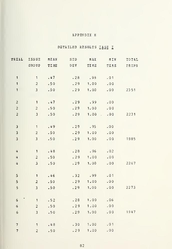
APPENDIX H
DETAILED RESULTS 3ASE I
TRIAL ISSUE MEAN STD MAX MIN TOTAL
GROUP TIME DEV TIME TIME TRIPS
1 1 .47 .28 .98 .01
1 2 .50 .29 1.00 .00
1 3 .50 .29 1.00 .00 2351
2 1 .47 .29 .99 .00
2 2 .50 .29 1.00 .00
2 3 .50 .29 1.00 . .00 2231
3 1 .49 .29 .95 .00
3 2 .50 .29 1.00 .00
3 3 .50 .29 1.00 .00 1385
4 1 .48 .28 .96 .02
4 2 .50 .29 1 .00 .00
4 3 .50 .29 1.00 .00 2267
5 1 .46 .32 .99 .01
5 2 .50 . 29 1.00 .00
5 3 .50 .29 1.00 .00 2273
•
6 1 .52 .28 1.00 .06
6 2 .50 .29 1 .00 .00
6 3 .50 .29 1.00 .00 1947
7 1 .48 .30 1.00 .01
7 2 .50 .29 1 .00 .00
82


50 29 1.00 00 2079
8 1 .50 .29 1.00 .00
8 2 .50 .29 1.00 .00
8 3 .50 .29 1.00 .00 2034
9 1 .52 .30 1.00 .00
9 2 .50 .29 1.00 .00
9 3 .50 .29 1.00 .00 2314
10*
CAS E II
IAL ISSUE MEAN SID MAX MIN TOTAL
GROUP TIME DEY TIME TIME TRIPS
1*
2 1 3. 61 1 . 91 6.33 .17
2 2 3.60 2.00 7.00 .00
2 3 3. 61 1.99 7.00 .00 332
3 1 3.60 1. 71 6.93 .04
3 2 3.43 2.01 7.00 .00
3 3 3. 41 2.00 7.00 .00 336
4*
5 1 3. 47 2.02 6.97 .02
5 2 3.51 2.05 7.00 .00
5 3 3.49 2.07 7.00 .00 341
6 1 3.45 1.88 6.90 .06
6 2 3.52 2.00 7.00 .00
6 3 3.53 2.01 7.00 .00 283
7*
8 1 3. 27 1. 91 6.96 .43
8 2 3.52 2.02 7.00 .00
8 3 3. 52 2.01 7.00 .00 303
9*
83


10*
CASE III
TRIAL ISSUE MEAN STD MAX MIN TOTAL
GROUP TIME DEV TIME TIME TRIPS
1*
2 1 . 00 .00 .00 .00
2 2 2.92 1. 99 7.00 .00
2 3 2. 93 1. 99 7.00 .00 403
3 1 . 00 .00 .00 . 00
3 2. 91 2.00 7.00 .00
3 3 2.89 1.98 7.00 .00 430
4 1 . 00 . 00 .00 .00
4 2 2. 90 1.98 7.00 . 00
4 3 2.89 1.98 7.00 .00 413
5 1 .CO . 00 .00 .00
5 n*. 2. 96 1. 99 7.00 .00
5 3 2.93 2.01 7.00 .00 397
6 1 . 00 .00 .00 .00
6 2 2. 80 1 . 95 7.00 .00
6 3 2.78 1. 95 7.00 . 00 370
7*
8 1 .00 . 00 .00 .00
8 2 3. 04 2.02 7.00 .00
8 3 3.04 2.01 7.00 . 00 353
9*
10*
CASE IV
TRIAL ISSUE MEAN STD MAX MIN TOTAL
GROUP TIME DEV TIME TIME TRIPS
84


1
1
1
2
2
2
3
3
3
4
4
4
5
5
5
6
6
6
7
7
7
a
8
8
9
9
9
1 .00
2 .49
3 .51
1 .00
2 .48
3 .52
1 .00
2 .49
3 .52
1 .00
2 .48
3 .53
1 .00
2 .49
3 .52
1 .00
2 .49
3 .51
1 .00
2 .49
3 .52
1 .00
2 .49
3 .51
1 .00
2 .49
3 .52
00 .00 .00
29 1 .00 .00
38 6.69 .00
00 .00 .00
29 1.00 .00
41 6.95 .00
00 .00 .00
29 1.00 .00
38 6.98 .00
00 .00 .00
29 1.00 .00
42 6.89 .00
00 .00 .00
29 1 .00 .00
38 6.87 .00
00 .00 .00
29 1 .00 .00
37 6.91 .00
00 .CO .00
29 1 .00 .00
38 6.99 .00
00 .00 .00
29 1 .00 .00
36 6.93 .00
00 .00 .00
29 1 .00 .00
38 7.00 .00
1788
1865
1995
1901
1920
1690
1752
1797
2018
85


10*
^Results not available
exceeds 433,300 bytes.
Computer memory space required
86

LIST OF REFERENCES
1. Barksdule, G. L. and Mayer, W. B., TPS X A Text
Processing System, Naval Postgraduate School,
Monterey, California, 1976.
2. Chief of Naval Operations, QPNAV Instruction
4790 (series)f
Ships il§iSi§Il§SSS 1US Material
Man agement . Department of the Navy, Washington D. C.
,
1979.
3. Chief of Naval Operations, 0PNA7 Instruction
461 4
^
se rie s ) ,. Unifoci Material Movement and Issue
Priority S£stems Ii2WMIPS]_, Department of the Navy,
Washington, D. C, 1979.
4. Clark, and Disney, Probability an d Random Pro cesses
For Engineer s and Scientists, John Wiley and Sons,
Inc., New York, New York, 1970.
5. Conway R. W., Some Tactical Problems in Digital
Simulation, Management Science, Vol. 10, No. 1, Oct,
1963.
6. Degroot, Morris H., PlS^iSilitx and Statistics,
Addison-Wesley Publishing Company, Reading,
Massachusetts, 1975.
7. Fishraan, George S. , Principles of Discrete Event
Simulation, John Wiley and Sons, New York, New York,
1978.
8. Hernandez, E R, Jr.; and Gallitz, R. J, An Analysis
of the Oakland Naval Su£p_ly_ Center^s Bay_ krea Local
Del ivery System, Naval Postgraduate School, Monterey,
87

9.
10.
11 .
12.
13.
Califormia , 1976.
J.;Kiviat, P
JIMSC.•<r——.
—
1975.
SIM SCRIPT II..5,
Villanueva, a.; and Markowitz, H. M.
,
C\ZI, Inc., Los Angelas, California,
Naval Supply Systems Command, NAVSUP Pub^ 437, ,
Department of the Navy, Washington D. C.
Naval Supply Systems Command, UDAPS Mi lstr ip
Programs, UE0 2X OBO^ UBJM^ UJ2 8, , Department of the
Navy, Washington D. C.
Shannon, Robert E, Systems Simulation the Art and
Science, Prsntice-Hall , Inc., Englewood Cliffs, New
Jersey, 1974.
i SIMSCRIPT ILi5 Reference Handboo k,
C.A.C.I. Inc, Los Angeles, California, 1976.
38

INITIAL DISTRIBUTION LIST
No. Copies
1. Defense Logistics Studies 1
Information Exchange (DLSIE)
Fort Lee, Virginia 23801
2. Defense Documentation Center 2
Cameron Station
Alexandria, Virginia 22314
3. Library, Code 0142 2
Naval Postgraduate School
Monterey, California 93940
4. Department Chairman, Code 55 1
Department of Operations Research
Naval Postgraduate School
Monterey, California 93940
5. LCDR Gary J. Angelopoulos 1
10007 S» 126th Street
Miami, Florida 33176
6. Professor A. W. McMasters 5
Code 54Mg
Naval Postgraduate School
Monterey, California 93940
7. CDR Robert D. Grant 5
Code 08
Naval Supply Center Dakland
Oakland, California 94625
8. Mr. H. J. Lieberman 2
89


Code 0431B
Naval Supply Systems Command
Washington, O.C. 20376
90


IThesisA5^5 Angelopoulos ] 842.Ic.l
- i cImpact of U. S. naval
vessel movements withinSan Francisco Bay Area onNaval Supply Center Oak-land's transportation
an-
system.
I 2 NOV 82
» 2 NOV 823 Jun e
a
a-
2 8*314} -
2 84 31-
ThesisA5^5 Angelopoulosc.l
184272naval
within
Impact of U. Svessel movements
San Francisco Bay Area onNaval Supply Center Oak-land's transportationsystem.

thesA545
Impact of U.S. naval vessel movements wi
3 2768 000 99157 4DUDLEY KNOX LIBRARY