CFD WITH OPENSOURSE SOFTWARE

A COURSE AT CHALMERS UNIVERISTY OF TECHNOLOGY TAUGHT BY HÅKAN NILSSON

Project work:

Implementation of a turbulent inflow boundary condition for LES based on a vortex method

Developed for OpenFOAM-2.1.x

Author: NINA GALL JØRGENSEN

Peer reviewed by: SIMON TÖRNROS JELENA ANDRIC

Disclaimer: This is a student work, done as part of a course where OpenFOAM and some other OpenSource software are introduced to the students. Any reader should be aware that it might not be free of errors. Still, it might be useful for someone who would like to learn some details similar to the

ones presented in the report and in the accompanying files.

November 23, 2012

2

Contents

Chapter 1 - Introduction

1.1  Turbulent inflow boundary conditions in OpenFOAM-2.1.x ...................................... 4 

1.2  Background .................................................................................................................. 6 

1.2.1  2D vortex method ................................................................................................. 6 

1.2.2  Mean velocity and turbulent kinetic energy profiles ............................................ 7

Chapter 2 - Turbulent power law inflow boundary condition

2.1  Parabolic velocity inlet boundary condition .............................................................. 10 

2.2  Modifications to parabolic velocity BC ..................................................................... 11 

2.2.1  Changing parabolic velocity to power law velocity ........................................... 11 

2.2.2  Turbulent kinetic energy .................................................................................... 12 

2.2.3  Tangential fluctuations ....................................................................................... 13 

2.2.4  Total velocity at inlet boundary ......................................................................... 15 

2.3  Verification of BC ..................................................................................................... 15 

Conclusion…………………………………………………………………………………….17

References……………………………………………………………………………………..18

Appendix A……………………………………………………………………………………19

3

Chapter 1

Introduction

In Civil Engineering Large Eddy Simulations (LES) are used to predict unsteady flow patterns around buildings and wind loads on structures. As LES is an unsteady simulation it is necessary to introduce turbulent velocity time histories at the inlet boundary conditions (BC). These data should represent the turbulent atmospheric boundary layer flow upstream of the computational domain.

The most accurate method of producing inlet conditions that satisfy the Navier-Stokes equations is the use of precursor simulations. Here the upstream turbulent flow is simulated and the time varying data generated are then is introduced at the inlet of the actual simulation. However, these simulations are restricted to simple geometries and/or low Reynolds numbers as they are computationally expensive and require storage of large data amounts. To reduce the cost of the simulation of spatially evolving flows the inflow boundary is placed close upstream of the flow position of interest and some approximated turbulent velocity inflow BC are assigned to the inflow. The inflow data are obtained by methods that generate synthetic turbulence fields from some prescribed information of the statistics of the turbulent approaching flow. The simplest method is to superpose random fluctuations (or noise) on the mean velocity profile. This method is easy to interpret and only requires knowledge of the mean velocity and the turbulence level at the inlet. However, as the signals created are random no space- or time correlations exist and the flow lacks realistic turbulent structures. Furthermore, the energy spectrum is reproduces incorrectly as all scales have the same energy and contribute equally to the signal. The fluctuations therefore die out quickly downstream of the inlet due to the overload of energy in the small scales. This method is therefore not suitable for simulating fully developed turbulent atmospheric boundary layer flows. Other methods with some spatial and or temporal correlations where various physical requirements of the flow are met have been developed. Using a digital filtering procedure on random data or spectral methods where the time series are obtained by inverse fast Fourier transform of a prescribed spectrum are examples of such methods. A review of some methods can be found in Jarrin (2008). The aim of the work presented in this project is to create a new turbulent BC which generates a time-dependent fluctuating inlet velocity field for LES. The BC is based on a vortex method developed originally Sergent (2002) and adopted and implemented in the commercial CFD software ANSYS Fluent by Mathey et al. (2006). It is emphasized that, due to time restrictions, the method by Mathey is not fully implemented in this project and some

4

exclusions and assumptions to the method are made. The new BC powerLawTurbulentVelocity is created by modifying the existing inlet boundary

condition parabolicVelocity which can be found for OpenFOAM-1.5-dev. The

parabolicVelocity BC uses a function to create a 2D parabolic velocity profile from predefined velocity intensity. An alternative way of defining the velocity profiles at the inlet would be to map data values in specified points along the height of the inlet patch. This can be done with the timeVaryingMappedFixedValue boundary condition, which often is used to map experimentally obtained values to the inlet.

The first part of this report gives a short description of the turbulent inflow BCs available in OpenFOAM and the theory of the vortex method implemented and the second part can be seen as a tutorial explaining the implementation of the new BC in OpenFOAM-2.1.x.

1.1 Turbulent inflow boundary conditions in OpenFOAM-2.1.x

There are two ways of generating velocity inlet BC for LES in OpenFOAM-2.1.x; a recycling method and a random inflow generator. In the recycling method turbulent data are mapped from a plane positioned downstream of the inlet back to the inlet. This method is simpler to use than a precursor simulation as the mapping of data is performed in the actual simulation and storage of large datasets is avoided. However, the inlet and the mapping plane have to be placed far enough upstream of any disturbances in the flow. A tutorial for this BC (type mapped) can be found in $FOAM_TUTORIALS/incompressible/pisoFoam/les/ pitzDailyMapped. The inflow boundary condition for the pitzDailyMapped tutorial is shown in Figure 1 together with the required entries for the BC.

inlet { type mapped; value uniform (10 0 0); interpolationScheme cell; setAverage true; average (10 0 0); }

Figure 1. Mapped velocity boundary condition at inlet patch.

5

The turbulentInlet is a synthetic inflow BC generator where random noise is added to the specified inlet velocity from a defined turbulence level. Inlet velocity data generated by this BC are shown in Figure 2 for a 2D patch. No realistic synthetic BC’s are implemented in OpenFOAM-2.1.x as standard. However, Rostock University has implemented a turbulent generator where turbulent fluctuations are superimposed onto the mean velocity called inflowGenerator (Kornev et al., 2009). The method is based on the idea of turbulent flow being a motion of turbulent spots arising at random positions at random times. Data generated by this inlet BC at an inlet patch of a 3-D case is shown in Figure 3.

inlet { type turbulentInlet; referenceField uniform (10 0 0); fluctuationScale (0.02 0.01 0.01);value uniform (10 0 0) }

Figure 2. turbulentInlet velocity boundary condition at inlet patch.

inlet { overlap 0.5; L 0.01; eta 1e-04; Cl 6.783; Ceta 0.4; type inflowGenerator<homogeneousTurbulence>; referenceField uniform (10 0 0); fluctuationScale (0.2 0.1 0.1); value uniform (10 0 0);}

Figure 3. inflowGenerator velocity boundary condition at inlet patch.

6

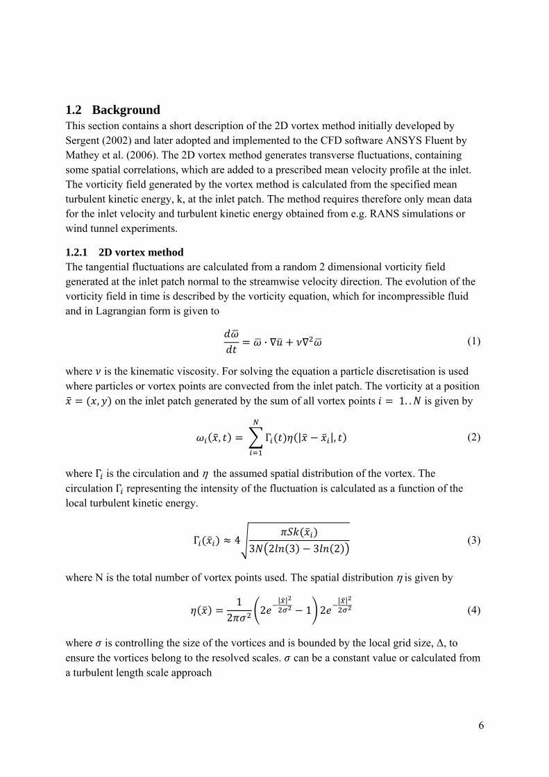
1.2 Background This section contains a short description of the 2D vortex method initially developed by Sergent (2002) and later adopted and implemented to the CFD software ANSYS Fluent by Mathey et al. (2006). The 2D vortex method generates transverse fluctuations, containing some spatial correlations, which are added to a prescribed mean velocity profile at the inlet. The vorticity field generated by the vortex method is calculated from the specified mean turbulent kinetic energy, k, at the inlet patch. The method requires therefore only mean data for the inlet velocity and turbulent kinetic energy obtained from e.g. RANS simulations or wind tunnel experiments.

1.2.1 2D vortex method The tangential fluctuations are calculated from a random 2 dimensional vorticity field generated at the inlet patch normal to the streamwise velocity direction. The evolution of the vorticity field in time is described by the vorticity equation, which for incompressible fluid and in Lagrangian form is given to

· (1)

where is the kinematic viscosity. For solving the equation a particle discretisation is used where particles or vortex points are convected from the inlet patch. The vorticity at a position

, on the inlet patch generated by the sum of all vortex points 1. . is given by

, Γ | |, (2)

where Γ is the circulation and η the assumed spatial distribution of the vortex. The circulation Γ representing the intensity of the fluctuation is calculated as a function of the local turbulent kinetic energy.

Γ 43 2 3 3 2

(3)

where N is the total number of vortex points used. The spatial distribution η is given by

1

22

| |1 2

| | (4)

where is controlling the size of the vortices and is bounded by the local grid size, Δ, to ensure the vortices belong to the resolved scales. can be a constant value or calculated from a turbulent length scale approach

7

/ /

(5)

The resulting discretisation for the tangential velocity field , is obtained by using the Biot-Savart law which relates the velocity to the vorticity.

1

2Γ

| |1

| | | | (6)

Hence each velocity position is effected by all vortex points to different degree depending on the distance between the position and the vortex position , . The vector

0, 0, 1 is the unit vector in the streamwise direction.

1.2.2 Mean velocity and turbulent kinetic energy profiles For atmospheric boundary layer flows the logarithmic law is the most accurate mathematical function for describing the variation of the mean wind velocity with height above the ground. Considering only a height range covering most structures near the ground and urban areas with rough terrain the mean velocity as a function of height, z, above ground can be defined as:

(7)

where is the friction velocity, 0 is a measure of the roughness of the ground surface, 0 is a zero-plane displacement obtained from the general rooftop height of the considered urban area and is the von Kármán constant.

An alternative to the logarithmic law often used in wind engineering is the power law. This profile has no theoretical basis but is easy to integrate and can in contrast to the logarithmic law be evaluated for heights below 0.

10

(8)

where is the exponent defining the terrain roughness and is the mean wind velocity at height 10m above ground. The exponent can be related to and the height above the ground where the power law is matching the logarithmic law, .

1

/ (9)

The turbulence intensity, which is a ratio of the standard deviation to the mean value of the fluctuating velocity, can be related to .

8

1

/ (10)

The turbulent kinetic energy is calculated from the streamwise mean velocity, U, and the streamwise turbulence intensity, .

32

(11)

9

Chapter 2

Turbulent power law inflow boundary condition

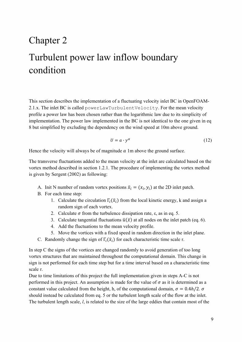
This section describes the implementation of a fluctuating velocity inlet BC in OpenFOAM-2.1.x. The inlet BC is called powerLawTurbulentVelocity. For the mean velocity profile a power law has been chosen rather than the logarithmic law due to its simplicity of implementation. The power law implemented in the BC is not identical to the one given in eq 8 but simplified by excluding the dependency on the wind speed at 10m above ground.

· (12)

Hence the velocity will always be of magnitude 1m above the ground surface.

The transverse fluctuations added to the mean velocity at the inlet are calculated based on the vortex method described in section 1.2.1. The procedure of implementing the vortex method is given by Sergent (2002) as following:

A. Init N number of random vortex positions , at the 2D inlet patch. B. For each time step:

1. Calculate the circulation Γ from the local kinetic energy, k and assign a random sign of each vortex.

2. Calculate from the turbulence dissipation rate, ε, as in eq. 5. 3. Calculate tangential fluctuations at all nodes on the inlet patch (eq. 6). 4. Add the fluctuations to the mean velocity profile. 5. Move the vortices with a fixed speed in random direction in the inlet plane.

C. Randomly change the sign of Γ for each characteristic time scale τ.

In step C the signs of the vortices are changed randomly to avoid generation of too long vortex structures that are maintained throughout the computational domain. This change in sign is not performed for each time step but for a time interval based on a characteristic time scale τ. Due to time limitations of this project the full implementation given in steps A-C is not performed in this project. An assumption is made for the value of as it is determined as a constant value calculated from the height, h, of the computational domain, 0.4 /2. should instead be calculated from eq. 5 or the turbulent length scale of the flow at the inlet. The turbulent length scale, l, is related to the size of the large eddies that contain most of the

10

energy and can be estimated to 0.4 for boundary layer flows. Where the boundary layer height, δ, is approximately the height from the ground where the velocity has reached the free stream velocity. In step B-5 the vortices are not moved with a fixed speed in the inlet patch but new random vortex positions are generated for each time step. As the vortices are moved randomly and not by a fixed speed the space correlations of the velocity field will be lost. Instead the vortex points should be moved a fixed distance · ∆ based on the time step and a constant velocity or a velocity depending on the vortex position in the inlet patch. Finally, step C is excluded and the sign of the vortices are always kept the same. For realistic use of the implemented BC the work in this project should be extended where the mentioned exclusions should be implemented. In the following chapters the implementation of the BC described above is performed.

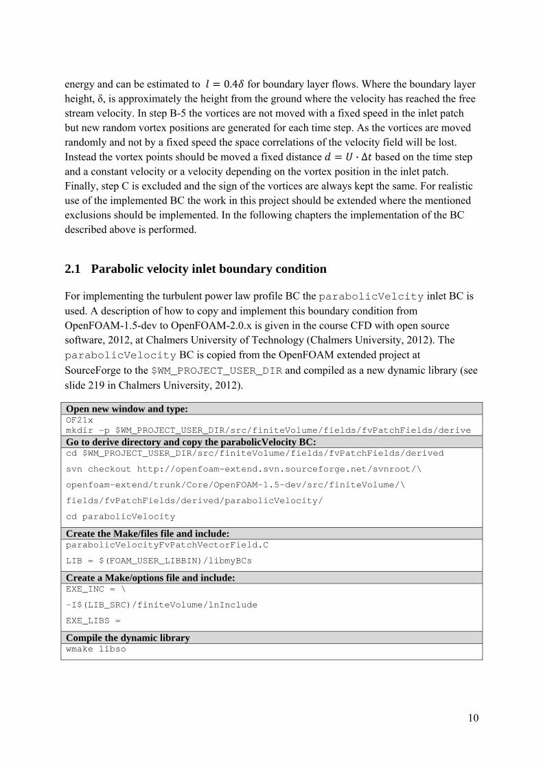
2.1 Parabolic velocity inlet boundary condition

For implementing the turbulent power law profile BC the parabolicVelcity inlet BC is used. A description of how to copy and implement this boundary condition from OpenFOAM-1.5-dev to OpenFOAM-2.0.x is given in the course CFD with open source software, 2012, at Chalmers University of Technology (Chalmers University, 2012). The parabolicVelocity BC is copied from the OpenFOAM extended project at

SourceForge to the $WM_PROJECT_USER_DIR and compiled as a new dynamic library (see slide 219 in Chalmers University, 2012).

Open new window and type: OF21x mkdir -p $WM_PROJECT_USER_DIR/src/finiteVolume/fields/fvPatchFields/derive Go to derive directory and copy the parabolicVelocity BC: cd $WM_PROJECT_USER_DIR/src/finiteVolume/fields/fvPatchFields/derived

svn checkout http://openfoam-extend.svn.sourceforge.net/svnroot/\

openfoam-extend/trunk/Core/OpenFOAM-1.5-dev/src/finiteVolume/\

fields/fvPatchFields/derived/parabolicVelocity/

cd parabolicVelocity

Create the Make/files file and include: parabolicVelocityFvPatchVectorField.C

LIB = $(FOAM_USER_LIBBIN)/libmyBCs

Create a Make/options file and include: EXE_INC = \

-I$(LIB_SRC)/finiteVolume/lnInclude

EXE_LIBS =

Compile the dynamic library wmake libso

11

For any case in OpenFOAM where you want to use the parabolic velocity BC at your inlet you have to specify the parabolicVelocity type for the inlet patch in the 0/U

directory. Furthermore, for the OpenFOAM solver to recognize the parabolicVelocity

BC the library for the BC must be defined by adding the line libs(“libmyBCs.so”); to

the system/controlDict file. For demonstration the parabolicVelocity inlet BC

is shown in Figure 4, used at the inlet patch for a 2D case. The required entries in the 0/U file are shown in the figure to the left.

inlet { type parabolicVelocity; n (1 0 0); // Flow direction y (0 1 0); // Profile direction maxValue 1; // Max value of parabolvalue uniform (0 0 0); // Dummy for paraFoam }

Figure 4. Parabolic velocity boundary condition at inlet patch with maxValue = 1.

For creating the power law inlet BC the parabolicVelocity BC is copied to

powerLawTurbulentVelocity and the following modifications are done.

Rename the .C and .H files from parabolic to powerLawTurbulent Change parabolic to powerLawTurbulent everywhere in the .C and .H files Modify the Make/files file powerLawTurbulentVelocityFvPatchVectorField.C

LIB = $(FOAM_USER_LIBBIN)/libmypowerLawTurbulent

Compile the new dynamic library

2.2 Modifications to parabolic velocity BC

In the following the modifications to the powerLawTurbulentVelocity.H and the

powerLawTurbulentVelocity.C files are described.

2.2.1 Changing parabolic velocity to power law velocity Lines for the new private data a and alpha are added everywhere in the

powerLawTurbulentVelocity.H and powerLawTurbulentVelocity.C file.

These data are scalars and can be implemented in the same way as the original

12

maxValue in parabolicVelocity. All lines for maxValue data are erased or overwritten.

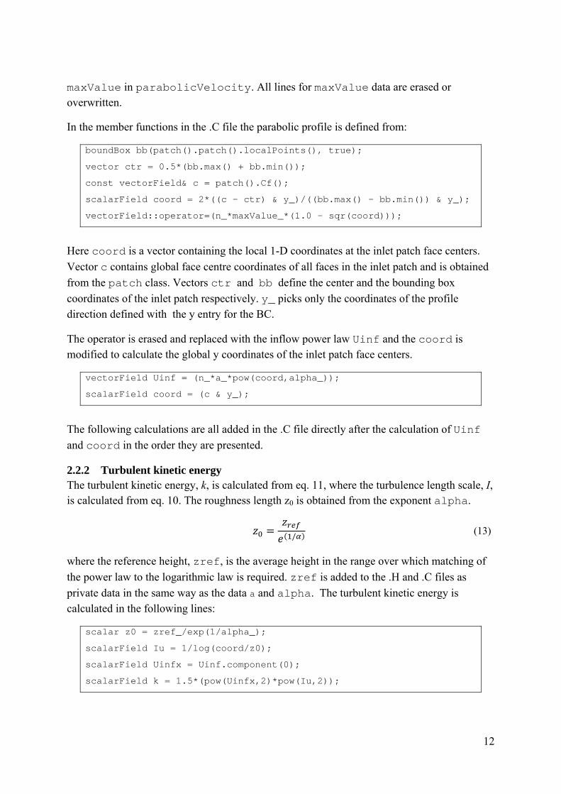
In the member functions in the .C file the parabolic profile is defined from:

boundBox bb(patch().patch().localPoints(), true);

vector ctr = 0.5*(bb.max() + bb.min());

const vectorField& c = patch().Cf();

scalarField coord = 2*((c - ctr) & y_)/((bb.max() - bb.min()) & y_);

vectorField::operator=(n_*maxValue_*(1.0 - sqr(coord)));

Here coord is a vector containing the local 1-D coordinates at the inlet patch face centers.

Vector c contains global face centre coordinates of all faces in the inlet patch and is obtained

from the patch class. Vectors ctr and bb define the center and the bounding box

coordinates of the inlet patch respectively. y_ picks only the coordinates of the profile direction defined with the y entry for the BC.

The operator is erased and replaced with the inflow power law Uinf and the coord is modified to calculate the global y coordinates of the inlet patch face centers.

vectorField Uinf = (n_*a_*pow(coord,alpha_));

scalarField coord = (c & y_);

The following calculations are all added in the .C file directly after the calculation of Uinf

and coord in the order they are presented.

2.2.2 Turbulent kinetic energy The turbulent kinetic energy, k, is calculated from eq. 11, where the turbulence length scale, I, is calculated from eq. 10. The roughness length z0 is obtained from the exponent alpha.

/ (13)

where the reference height, zref, is the average height in the range over which matching of

the power law to the logarithmic law is required. zref is added to the .H and .C files as

private data in the same way as the data a and alpha. The turbulent kinetic energy is calculated in the following lines:

scalar z0 = zref_/exp(1/alpha_);

scalarField Iu = 1/log(coord/z0);

scalarField Uinfx = Uinf.component(0);

scalarField k = 1.5*(pow(Uinfx,2)*pow(Iu,2));

13

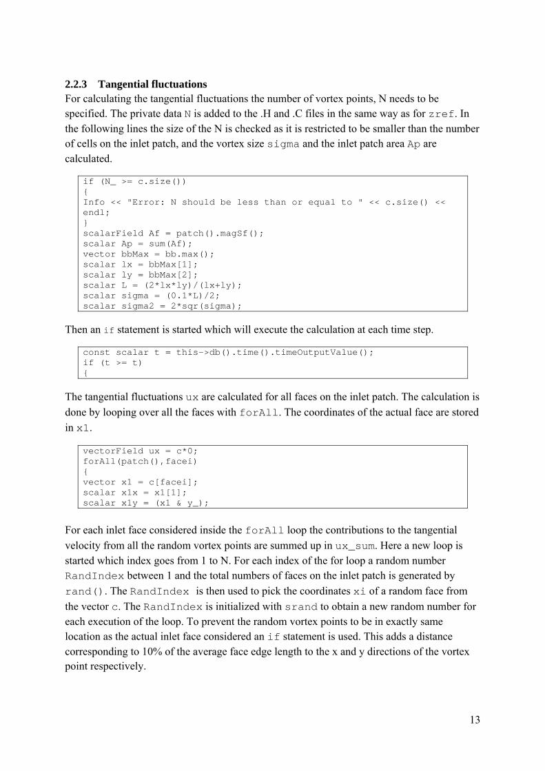
2.2.3 Tangential fluctuations For calculating the tangential fluctuations the number of vortex points, N needs to be specified. The private data N is added to the .H and .C files in the same way as for zref. In the following lines the size of the N is checked as it is restricted to be smaller than the number of cells on the inlet patch, and the vortex size sigma and the inlet patch area Ap are calculated.

if (N_ >= c.size()) { Info << "Error: N should be less than or equal to " << c.size() << endl; } scalarField Af = patch().magSf(); scalar Ap = sum(Af); vector bbMax = bb.max(); scalar lx = bbMax[1]; scalar ly = bbMax[2]; scalar L = (2*lx*ly)/(lx+ly); scalar sigma = (0.1*L)/2; scalar sigma2 = 2*sqr(sigma);

Then an if statement is started which will execute the calculation at each time step.

const scalar t = this->db().time().timeOutputValue(); if (t >= t) {

The tangential fluctuations ux are calculated for all faces on the inlet patch. The calculation is

done by looping over all the faces with forAll. The coordinates of the actual face are stored

in x1.

vectorField ux = c*0; forAll(patch(),facei) { vector x1 = c[facei]; scalar x1x = x1[1]; scalar x1y = (x1 & y_);

For each inlet face considered inside the forAll loop the contributions to the tangential

velocity from all the random vortex points are summed up in ux_sum. Here a new loop is started which index goes from 1 to N. For each index of the for loop a random number RandIndex between 1 and the total numbers of faces on the inlet patch is generated by

rand(). The RandIndex is then used to pick the coordinates xi of a random face from

the vector c. The RandIndex is initialized with srand to obtain a new random number for each execution of the loop. To prevent the random vortex points to be in exactly same location as the actual inlet face considered an if statement is used. This adds a distance corresponding to 10% of the average face edge length to the x and y directions of the vortex point respectively.

14

srand (time(NULL) ); vector ux_sum = vector(0, 0, 0); for (int iter = 1; iter <= N_; iter ++) { int RandIndex = rand() % c.size(); vector xi = c[RandIndex]; if (xi == x1) { scalar Lxi = sqrt(patch().magSf()[iter]); scalar addxi = 0.1*Lxi; xi[1] = xi[1]+addxi; xi[2] = xi[2]+addxi; } scalar xix = xi[1]; scalar xiy = (xi & y_);

After obtaining the coordinates of the random vortex point the circulation, gamma given in

eq. 3 is calculated based on the local level of the turbulent kinetic energy ks and the total

inlet patch area Ap. As ks is obtained in the face centers there is a small discrepancy in the

cases where xi has been moved corresponding to the if statement described above.

scalar dist = sqr(x1x-xix)+sqr(x1y-xiy); vector xx = xi-x1; scalar ks = k[RandIndex]; scalar gamma = 4*sqrt((Foam::constant::mathematical::pi*Ap*ks)/ (3*N_*0.117783035656383));

From gamma the tangential fluctuation ux1 given in eq. 6 is calculated and finally summed

up for all vortex points ux_sum. In the calculations of ux1, sigma, used to control the size

of the vortex points, is bounded by the local face size delta.

scalar delta = sqrt(patch().magSf()[RandIndex]); if (sigma <= delta) { sigma = delta; sigma2 = 2*sqr(sigma); } vector z1 = vector(1,0,0); vector ux1 = (gamma*((xx ^ z1)/dist)*(1-exp(- dist/sigma2))*exp(-dist/sigma2)); ux_sum += ux1; }

The tangential fluctuations for each face on the inlet patch are stored in a vectorField ux before the forAll loop is closed.

ux[facei] = (1/(2*3.141592653589793))*ux_sum; }

15

2.2.4 Total velocity at inlet boundary At the end of the member functions the operator is defined as the mean power law velocity profile plus the tangential fluctuations and the if statement controlling the execution at each time step is closed.

vectorField::operator=(Uinf+ux); }

The new timeVaryingMappedFixedValue BC is the compiled with wmake libso.

2.3 Verification of BC

The use of the timeVaryingMappedFixedValue BC is demonstrated on a case

simulating flow over a smooth ground surface called boxPowerLawTurbulentLES. The purpose of this simulation is to verify the implementation of the BC and see if it runs properly on a case without any errors. The case is 3 dimensional with x, y and z coordinates in streamwise, spanwise and vertical directions respectively. The geometry and the boundary conditions of the case are shown in Figure 5. For the case the oneEqEddy LES model and

the transient pisoFoam solver are used. For creating the case the pitzDaily tutorial in /OpenFOAM-2.1.x/tutorials/incompressible/pisoFoam/les/ pitzDaily is copied into the run folder and renamed to

timeVaryingMappedFixedValue. In the system directory all original settings are kept

and the line libs ("libmypowerLawTurbulent.so"); is added to the

system/controlDict file for enabling the use of the powerLawTurbulent BC.

The upper- and side walls of the computational domain are defined as symmetryPlane and the bottom as a wall with zero velocity and zeroGradient pressure. A boundary condition for k is also needed in the 0 directory. This is due to how the LES models are implemented in OpenFOAM but k is not explicitly needed by the LES model itself.

Figure 5. Geometry of test case.

inlet

symmetryPlane

wall

outlet

16

The mesh created in the blockMesh file in the constant directory and the boundary and

initial conditions defined in the 0 directory have to be modified to obtain the geometry and

mesh shown in Figure 5. The new blockMesh and boundary condition files are shown in

Appendix A. For running the case the commands blockMesh and pisoFoam are executed from the case directory in a terminal.

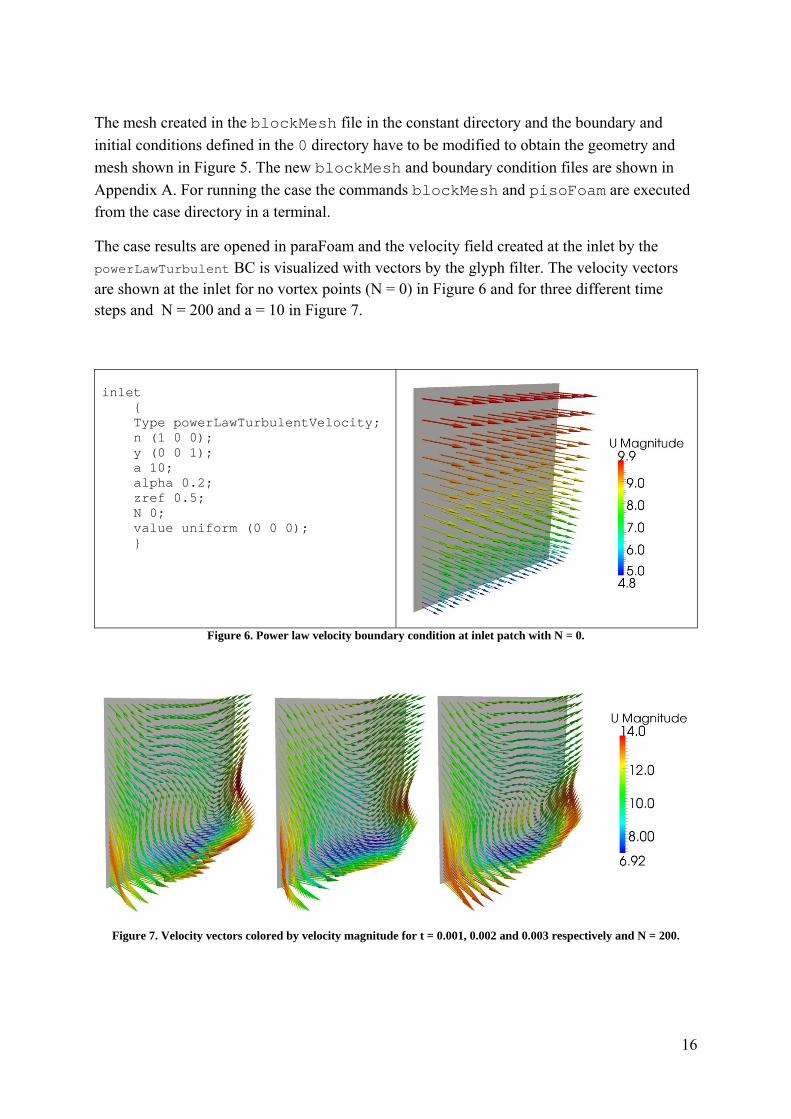
The case results are opened in paraFoam and the velocity field created at the inlet by the powerLawTurbulent BC is visualized with vectors by the glyph filter. The velocity vectors are shown at the inlet for no vortex points (N = 0) in Figure 6 and for three different time steps and N = 200 and a = 10 in Figure 7.

inlet { Type powerLawTurbulentVelocity; n (1 0 0); y (0 0 1); a 10; alpha 0.2; zref 0.5; N 0; value uniform (0 0 0); }

Figure 6. Power law velocity boundary condition at inlet patch with N = 0.

Figure 7. Velocity vectors colored by velocity magnitude for t = 0.001, 0.002 and 0.003 respectively and N = 200.

17

Conclusion A time-varying turbulent power law inflow BC for use with LES models have been implemented in OpenFOAM-2.1.x. The calculation of the fluctuations in the BC is based on a 2D vortex method with some simplifications. The implementation and compilation of the BC has been verified on a case where the oneEqEddy LES model and the pisoFoam solver are used. For a qualitative validation of the inflow data produced by the BC it should be used for a correct LES of a turbulent atmospheric boundary layer flow. As it is CPU expensive to run LES such a validation was not performed due to the given time frame of this project.

For obtaining space correlation of the tangential fluctuations and correct size of the vortices created in the BC it is necessary to implement the simplifications made to steps A-C of the 2D vortex method described in beginning of Chapter 2. Furthermore, for a realistic inflow BC it would be necessary to implement streamwise fluctuations that could be added to the mean velocity. For comparison data obtained by the vortex method inflow BC implemented in the commercial CFD code ANSYS Fluent could be used.

18

References Chalmers University, 2012. How to implement new boundary condition, lecture slides in

Msc/PhD course in CFD with OpenSource software. http://www.tfd.chalmers.se/~hani/kurser/OS_CFD/implementBoundaryCondition.pdf

Kornev N., Shchukin E., Taranov E., Kröger H., Turnow J., Hassel E., 2009. Development and Implementation of Inflow Generator for LES and DNS applications in OpenFOAM. Open Source CFD International Conference 2009, Barcelona, Spain.

Mathey F., Cokljat D., Pierre J., Sergent E., 2006. Assessment of the vortex method for Large Eddy Simulation inlet conditions. Progress in Computational Fluid Dynamics, Vol. 6, Nos. 1/2/3.

Jarrin N., 2008. Synthetic inflow boundary conditions for the numerical simulation of turbulence. PhD thesis, University of Manchester, Faculty of Engineering and Physical Sciences, http://cfd.mace.manchester.ac.uk/CfdTm/ThesesDissertations.

Sergent, M.E. (2002) Vers une Méthodologie de Couplage Entre la Simulation des Grandes Echelles et les Modèles Statistiques, Phd Thesis, Ecole Central de Lyon.

19

Appendix A BlockMeshDict Replace the original file from the pitzDaily tutorial with the following lines.

//convertToMeters 0.001; vertices ( (0 0 0) (2 0 0) (2 1 0) (0 1 0) (0 0 1) (2 0 1) (2 1 1) (0 1 1) ); blocks ( hex (0 1 2 3 4 5 6 7) (40 20 30) simpleGrading (1 1 4) ); edges ( ); boundary ( inlet { type patch; faces ( (0 4 7 3) ); } outlet { type patch; faces ( (2 6 5 1) ); } backWall { type symmetryPlane; faces ( (3 7 6 2) ); } frontWall {

20

type symmetryPlane; faces ( (1 5 4 0) ); } lowerWall { type wall; faces ( (0 3 2 1) ); } upperWall { type symmetryPlane; faces ( (4 5 6 7) ); } ); mergePatchPairs ( );

21

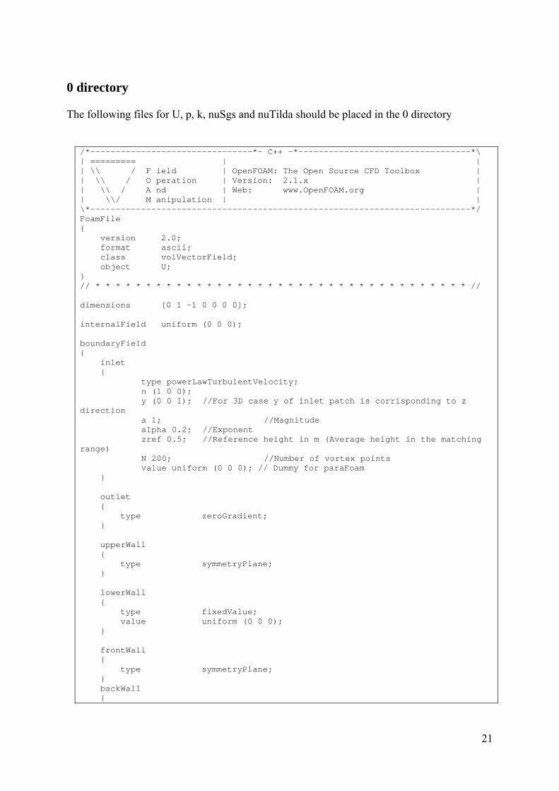
0 directory The following files for U, p, k, nuSgs and nuTilda should be placed in the 0 directory

/*--------------------------------*- C++ -*----------------------------------*\ | ========= | | | \\ / F ield | OpenFOAM: The Open Source CFD Toolbox | | \\ / O peration | Version: 2.1.x | | \\ / A nd | Web: www.OpenFOAM.org | | \\/ M anipulation | | \*---------------------------------------------------------------------------*/ FoamFile { version 2.0; format ascii; class volVectorField; object U; } // * * * * * * * * * * * * * * * * * * * * * * * * * * * * * * * * * * * * * // dimensions [0 1 -1 0 0 0 0]; internalField uniform (0 0 0); boundaryField { inlet { type powerLawTurbulentVelocity; n (1 0 0); y (0 0 1); //For 3D case y of inlet patch is corrisponding to z direction a 1; //Magnitude alpha 0.2; //Exponent zref 0.5; //Reference height in m (Average height in the matching range) N 200; //Number of vortex points value uniform (0 0 0); // Dummy for paraFoam } outlet { type zeroGradient; } upperWall { type symmetryPlane; } lowerWall { type fixedValue; value uniform (0 0 0); } frontWall { type symmetryPlane; } backWall {

22

type symmetryPlane; } } // ************************************************************************* //

/*--------------------------------*- C++ -*----------------------------------*\ | ========= | | | \\ / F ield | OpenFOAM: The Open Source CFD Toolbox | | \\ / O peration | Version: 2.1.x | | \\ / A nd | Web: www.OpenFOAM.org | | \\/ M anipulation | | \*---------------------------------------------------------------------------*/ FoamFile { version 2.0; format ascii; class volScalarField; object p; } // * * * * * * * * * * * * * * * * * * * * * * * * * * * * * * * * * * * * * // dimensions [0 2 -2 0 0 0 0]; internalField uniform 0; boundaryField { inlet { type zeroGradient; } outlet { type fixedValue; value uniform 0; } upperWall { type symmetryPlane; } lowerWall { type zeroGradient; } frontWall { type symmetryPlane; } backWall { type symmetryPlane; } } // ************************************************************************* //

23

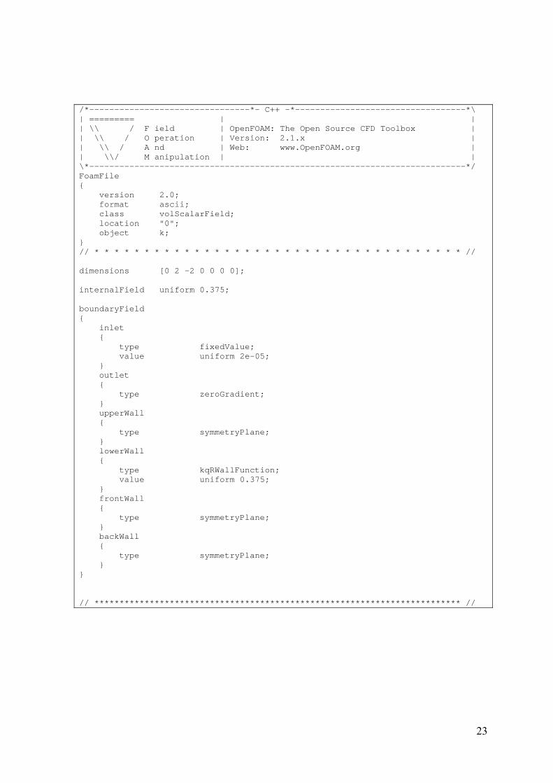
/*--------------------------------*- C++ -*----------------------------------*\ | ========= | | | \\ / F ield | OpenFOAM: The Open Source CFD Toolbox | | \\ / O peration | Version: 2.1.x | | \\ / A nd | Web: www.OpenFOAM.org | | \\/ M anipulation | | \*---------------------------------------------------------------------------*/ FoamFile { version 2.0; format ascii; class volScalarField; location "0"; object k; } // * * * * * * * * * * * * * * * * * * * * * * * * * * * * * * * * * * * * * // dimensions [0 2 -2 0 0 0 0]; internalField uniform 0.375; boundaryField { inlet { type fixedValue; value uniform 2e-05; } outlet { type zeroGradient; } upperWall { type symmetryPlane; } lowerWall { type kqRWallFunction; value uniform 0.375; } frontWall { type symmetryPlane; } backWall { type symmetryPlane; } } // ************************************************************************* //

24

/*--------------------------------*- C++ -*----------------------------------*\ | ========= | | | \\ / F ield | OpenFOAM: The Open Source CFD Toolbox | | \\ / O peration | Version: 2.1.x | | \\ / A nd | Web: www.OpenFOAM.org | | \\/ M anipulation | | \*---------------------------------------------------------------------------*/ FoamFile { version 2.0; format ascii; class volScalarField; object nuSgs; } // * * * * * * * * * * * * * * * * * * * * * * * * * * * * * * * * * * * * * // dimensions [0 2 -1 0 0 0 0]; internalField uniform 0; boundaryField { inlet { type zeroGradient; } outlet { type zeroGradient; } upperWall { type symmetryPlane; } lowerWall { type zeroGradient; } frontWall { type symmetryPlane; } backWall {

25

type symmetryPlane; } } // ************************************************************************* //

/*--------------------------------*- C++ -*----------------------------------*\ | ========= | | | \\ / F ield | OpenFOAM: The Open Source CFD Toolbox | | \\ / O peration | Version: 2.1.x | | \\ / A nd | Web: www.OpenFOAM.org | | \\/ M anipulation | | \*---------------------------------------------------------------------------*/ FoamFile { version 2.0; format ascii; class volScalarField; object nuTilda; } // * * * * * * * * * * * * * * * * * * * * * * * * * * * * * * * * * * * * * // dimensions [0 2 -1 0 0 0 0]; internalField uniform 0; boundaryField { inlet { type fixedValue; value uniform 0; } outlet { type zeroGradient; } upperWall { type zeroGradient; } lowerWall { type zeroGradient; }

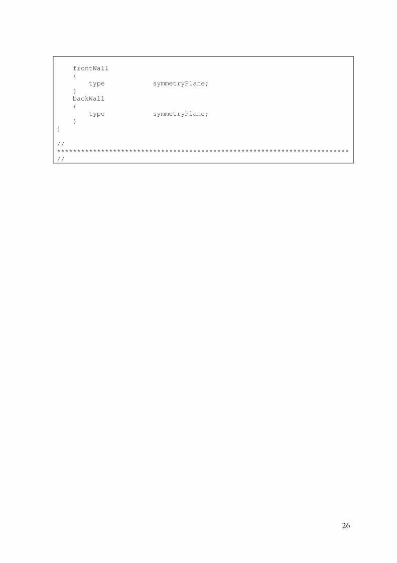
26

frontWall { type symmetryPlane; } backWall { type symmetryPlane; } } // ************************************************************************* //