implementation of wifire model in opnetsri/students/anirudha-thesis.pdf · implementation of wifire...
TRANSCRIPT

Implementation of WiFiRe Model inOPNET
A WiMAX-like MAC over WiFi PHY
Dissertation
submitted in partial fulfilment of the requirements
for the degree of
Master of Technology
by
Anirudha Bodhankar
(Roll no. 04329003)
under the guidance of
Prof. Sridhar Iyer
Kanwal Rekhi School of Information Technology
Indian Institute of Technology Bombay
2006


Dissertation Approval Sheet
This is to certify that the dissertation entitled
Implementation of WiFiRe Model inOPNET
A WiMAX-like MAC over WiFi PHY
by
Anirudha Bodhankar
(Roll no. 04329003)
is approved for the degree of Master of Technology.
Prof. Sridhar Iyer
(Supervisor)
Prof. Om Damani
(Internal Examiner)
Prof. Ashwin Gumaste
(Additional Internal Examiner)
Prof. Vishal Sharma
(Chairperson)
Date:
Place:
iii

INDIAN INSTITUTE OF TECHNOLOGY BOMBAY
CERTIFICATE OF COURSE WORK
This is to certify that Mr. Anirudha Bodhankar was admitted to the candidacy
of the M.Tech. Degree and has successfully completed all the courses required for the
M.Tech. Programme. The details of the course work done are given below.
Sr.No. Course No. Course Name Credits
Semester 1 (Jul – Nov 2004)
1. IT601 Mobile Computing 6
2. HS699 Communication and Presentation Skills (P/NP) 4
3. IT603 Data Base Management Systems 6
4. IT619 IT Foundation Laboratory 10
5. IT623 Foundation course of IT - Part II 6
6. IT694 Seminar 4
Semester 2 (Jan – Apr 2005)
7. CS686 Object Oriented Systems 6
8. EE701 Introduction to MEMS (Institute Elective) 6
9. IT610 Quality of Service in Networks 6
10. IT628 Data Mining 6
11. IT680 Systems Lab. 6
Semester 3 (Jul – Nov 2005)
12. CS601 Algorithms and Complexity (Audit) -
13. CS681 Performance Evaluation of Computer Systems and Networks 6
M.Tech. Project
14. IT696 M.Tech. Project Stage - I (Jul 2005) 18
15. IT697 M.Tech. Project Stage - II (Jan 2006) 30
16. IT698 M.Tech. Project Stage - III (Jul 2006) 42
I.I.T. Bombay Dy. Registrar(Academic)
Dated:
v


vii
Abstract
The 802.11(WiFi) family of wireless communication is extremely popular for indoor
wireless networking. The chipsets are designed so that PHY and MAC layers are separate
and they are available off-the-shelf at low cost. Also it operates in 2.5GHz ISM band
which is license free spectrum avoiding licensing cost, hence is an attractive option for
long range communication in rural areas of developing countries.
However many problem occur when using 802.11 for outdoor long range (15-20 Km)
communication. The DCF mode does not support any quality of service, while PCF is not
suitable for large number of stations and long distance. The MAC is based on CSMA/CA
and is not efficient when the number of stations increases. Hence it is necessary to redesign
MAC while retaining the PHY. One approach for this is WiFiRe
WiFiRe replaces the MAC of 802.11 with the MAC similar to that of 802.16 MAC
which is suitable for long range communication. It also uses directional antennas and is
meant for a star topology. WiFiRe MAC at the Base Station is multi-sector MAC which
controls more than one 802.11 directional PHY.
The goal of this project is to implement the WiFiRe model in OPNET and analyse its
performance. The code developed is to be such that, it can be easily extended to a real
implementation.

Contents
Abstract vii
List of figures xi
1 Introduction 1
1.1 Background . . . . . . . . . . . . . . . . . . . . . . . . . . . . . . . . . . . 1
1.2 WiFiRe Approach . . . . . . . . . . . . . . . . . . . . . . . . . . . . . . . . 1
1.3 Problem Definition . . . . . . . . . . . . . . . . . . . . . . . . . . . . . . . 3
1.4 Solution Strategy . . . . . . . . . . . . . . . . . . . . . . . . . . . . . . . . 3
1.5 Contributions of this Project . . . . . . . . . . . . . . . . . . . . . . . . . . 3
2 Literature Survey 5
2.1 802.11b (Wi-Fi) . . . . . . . . . . . . . . . . . . . . . . . . . . . . . . . . . 5
2.1.1 MAC Layer . . . . . . . . . . . . . . . . . . . . . . . . . . . . . . . 5
2.1.2 Physical Layer . . . . . . . . . . . . . . . . . . . . . . . . . . . . . . 6
2.2 Overview of 802.16 . . . . . . . . . . . . . . . . . . . . . . . . . . . . . . . 7
2.2.1 Medium Access Control Layer . . . . . . . . . . . . . . . . . . . . . 7
2.2.2 Physical Layer . . . . . . . . . . . . . . . . . . . . . . . . . . . . . . 9
2.2.3 Scheduling Service Classes . . . . . . . . . . . . . . . . . . . . . . . 9
2.2.4 Radio Link Control . . . . . . . . . . . . . . . . . . . . . . . . . . . 10
2.3 WiFiRe MAC design . . . . . . . . . . . . . . . . . . . . . . . . . . . . . . 10
2.4 Related Literature . . . . . . . . . . . . . . . . . . . . . . . . . . . . . . . 11
3 Choice of Simulator 13
3.1 QualNet . . . . . . . . . . . . . . . . . . . . . . . . . . . . . . . . . . . . . 13
3.2 OPNET . . . . . . . . . . . . . . . . . . . . . . . . . . . . . . . . . . . . . 14
ix

x Contents
3.2.1 We chose OPNET because . . . . . . . . . . . . . . . . . . . . . . . 14
3.3 OPNET Overview . . . . . . . . . . . . . . . . . . . . . . . . . . . . . . . 14
3.3.1 Pipeline Stages in OPNET . . . . . . . . . . . . . . . . . . . . . . . 14
4 Modelling WiFiRe in OPNET 19
4.1 Overview of Model in OPNET . . . . . . . . . . . . . . . . . . . . . . . . . 19
4.2 Assumptions . . . . . . . . . . . . . . . . . . . . . . . . . . . . . . . . . . . 21
4.3 MAC State Diagrams . . . . . . . . . . . . . . . . . . . . . . . . . . . . . . 21
4.4 Base Station State Diagram . . . . . . . . . . . . . . . . . . . . . . . . . . 25
4.5 Subscriber Station State Diagram . . . . . . . . . . . . . . . . . . . . . . . 28
5 Scheduler 31
5.1 Interference Pattern . . . . . . . . . . . . . . . . . . . . . . . . . . . . . . . 31
5.2 Greedy Heuristic Scheduler [1] . . . . . . . . . . . . . . . . . . . . . . . . . 32
5.2.1 Notation and Terminology . . . . . . . . . . . . . . . . . . . . . . . 32
5.2.2 Example . . . . . . . . . . . . . . . . . . . . . . . . . . . . . . . . . 33
5.3 Scheduling Uplink flows . . . . . . . . . . . . . . . . . . . . . . . . . . . . 34
5.4 Preprocessing . . . . . . . . . . . . . . . . . . . . . . . . . . . . . . . . . . 36
5.4.1 Notation and Terminology . . . . . . . . . . . . . . . . . . . . . . . 36
6 Simulation Setup 39
6.1 Simulation Setup . . . . . . . . . . . . . . . . . . . . . . . . . . . . . . . . 39
6.2 Scenario . . . . . . . . . . . . . . . . . . . . . . . . . . . . . . . . . . . . . 39
7 Conclusion 43
7.1 Future Work . . . . . . . . . . . . . . . . . . . . . . . . . . . . . . . . . . . 43
Abbreviations 1
Bibliography 45
Acknowledgements 47

List of Figures
1.1 WiFiRe Network Topology . . . . . . . . . . . . . . . . . . . . . . . . . . . 2
2.1 Downlink Frame Structure . . . . . . . . . . . . . . . . . . . . . . . . . . . 8
2.2 Uplink Frame Structure . . . . . . . . . . . . . . . . . . . . . . . . . . . . 8
2.3 A Multi-Sector MAC controlling multiple sector . . . . . . . . . . . . . . . 11
3.1 Describing antenna pattern using Φ and Θ . . . . . . . . . . . . . . . . . . 13
4.1 Block diagram of the system . . . . . . . . . . . . . . . . . . . . . . . . . . 20
4.2 MAC State Diagram . . . . . . . . . . . . . . . . . . . . . . . . . . . . . . 22
4.3 State Diagram of Base Station) . . . . . . . . . . . . . . . . . . . . . . . . 26
4.4 State Diagram of the Subscriber station . . . . . . . . . . . . . . . . . . . 29
5.1 A antenna coverage and interference pattern for a six sector partitioned cell 31
5.2 Example scenario of the system . . . . . . . . . . . . . . . . . . . . . . . . 33
6.1 Scenario of simulation setup. The unit is in 5km. . . . . . . . . . . . . . . 40
6.2 Throughput vs Load. Y-axis is in bps, X-axis in 10Mbps . . . . . . . . . . 41
6.3 Throughput vs Delay of UGS flows. Y-axis is in seconds, X-axis in 10Mbps 41
6.4 Throughput vs Delay of BE flows. Y-axis is in seconds, X-axis in 10Mbps . 42
xi

Chapter 1
Introduction
1.1 Background
Deploying cellular networks or wired networks in rural areas in India is not a feasible
solution because high cost of deployment. So the option that WiFiRe [2] proposes is the
802.11 family of wireless technologies. This is possible because of structure of Indian
rural area, where there are very few high rise buildings in the terrain for several kilo-
metres. With widespread acceptance of the technology, open/inter-operable standard,
and competitive mass production, the equipment and chip sets are inexpensive. But, it
has been found that the IEEE 802.11b MAC layer is not suitable for long-range outdoor
communication network, especially for voice traffic. The DCF (Distributed Coordination
Function) mechanism in 802.11b MAC layer does not provide any delay guarantees, while
the PCF(Point Coordination Function) mechanism becomes inefficient with increase in
number of stations and distance. In addition to this, in order to operate over long dis-
tances, the 802.11b MAC would require significantly longer slot times, further reducing
its efficiency. WiFiRe employs a mechanism similar to the IEEE 802.16 MAC layer.
1.2 WiFiRe Approach
The main design goal of WiFiRe[2] is to enable the development of low-cost hardware and
network operations for outdoor communications in a rural area. This is possible because:
• WiFiRe system avoids frequency licensing costs by operating in the unlicensed 2.4
GHz frequency band
• WiFiRe uses the IEEE 802.11b PHY for its physical layer, due to the low cost and
1
2 Chapter 1. Introduction
easy availability of IEEE 802.11b PHY chipsets.
WiFiRe employs the DSSS based IEEE 802.11b PHY layer as the physical layer mod-
ule for RF control. This 802.11b PHY system is for operation in the 2.4 GHz band and
designed for a wireless LAN with 1 Mbps, 2 Mbps and 11 Mbps data payload commu-
nication capability. The PHY has a processing gain of at least 10 dB and uses different
baseband modulations to provide the various data rates. The typical transmission reach
of this 802.11b PHY is 300 meters. However, WiFiRe extends the transmission range to
15-20 Kilometres, by using
• A deployment strategy based on sectorized/directional antennas
• MAC based on IEEE 802.16 MAC layer
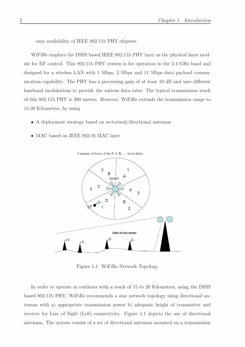
Figure 1.1: WiFiRe Network Topology
In order to operate in outdoors with a reach of 15 to 20 Kilometres, using the DSSS
based 802.11b PHY, WiFiRe recommends a star network topology using directional an-
tennas with a) appropriate transmission power b) adequate height of transmitter and
receiver for Line of Sight (LoS) connectivity. Figure 1.1 depicts the use of directional
antennas. The system consist of a set of directional antennas mounted on a transmission
1.3. Problem Definition 3
tower. Such a configuration would increase the reach of the 802.11b PHY to an outdoor
rural scenario.
1.3 Problem Definition
1. Understand functioning of WiFiRe protocol and its performance.
2. Develop simulation model which can be be used preliminary to the implementation.
1.4 Solution Strategy
1. Build a simulation model in OPNET.
2. Perform Experiments.
1.5 Contributions of this Project
The significant contributions of this work are:
1. Developing simulation model of WiFiRe in OPNET
2. Performing preliminary performance study
3. First step towards implementation of WiFiRe : It helped in identifying some pro-
tocol deficiencies in earlier drafts of the WiFiRe.
4. Minor improvements in the scheduling strategy


Chapter 2
Literature Survey
2.1 802.11b (Wi-Fi)
An overview of the IEEE 802.11b Wireless Lan (Wi-Fi) is presented in the following
section. The description reflects the various significant aspects of the standard’s PHY
and MAC layers.
2.1.1 MAC Layer
The 802.11 MAC, popularly known as WiFi provides two basic forms of channel access:
Distributed Coordination Function (DCF), and Point Coordination Function (PCF). DCF
is the most commonly used channel access mechanism which uses the Carrier Sense Mul-
tiple Access with collision avoidance (CSMA/CA) primitives. PCF is the centralised
channel arbitration method based on polling approach. DCF is mandatory part of the
standard, while PCF is optional.
In DCF method, each station senses the channel for a fixed duration called Distributed
InterFrame Space (DIFS). If the channel is idle for DIFS, then a random back-off value is
selected. The back-off value is decremented by one in each slot till the channel continues
to remain idle. Each station independently selects the back-off value from a range, Con-
gestion Window (0,CW-1). When the back-off reaches zero the station starts transmission
of data. For stations whose back-off count has not reached zero, the countdown is frozen
and they go into carrier sense phase waiting for the channel to be idle again for DIFS
duration. After DIFS, the station which has had a successful transmission chooses a new
random back-off value, while the others continue from the back-off value which was frozen
earlier. For each data packet transmitted, the destination sends a positive acknowledge-
5

6 Chapter 2. Literature Survey
ment at the MAC layer, after waiting for Short InterFrame Space (SIFS) duration. The
duration of SIFS is shorter than DIFS. It is possible that the back-off counter reaches zero
for more that two stations at the same time, resulting in collision of data. Absence of
acknowledgement is used to detect collisions. In this case, the stations which are involved
in the collision increase the range of Congestion Window using binary exponential back-
off procedure. The minimum value of CW is CWmin for the first attempt. In subsequent
attempts after collision, CW is doubled till it reaches CWmax.
The above mechanism of DCF is the basic DATA-ACK transmission of data. To
avoid collisions due to hidden nodes and exposed nodes in the network, the procedure is
extended by inclusion of a Request to Send (RTS) and Clear to Send (CTS) packets for a
RTS-CTS-DATA-ACK communication. This is also known as Virtual Carrier Sense. RTS
is sent by the transmitting node, and if the receiving node is willing to receive the data,
it replies with a CTS packet. There is waiting period of SIFS between each packet to
allow the transceivers at the stations to switch from transmitting mode to receiving mode
and vice-versa. Both the RTS and CTS packets contain expected duration of the data
transfer. All nodes which overhear the RTS and CTS packets remain idle for the duration
of the data transfer, hence allowing data packets to be transmitted without collisions.
2.1.2 Physical Layer
Depending on the current infrastructure and the distance between the sender and receiver
802.11b system offers 11, 5.5 , 2 or 1 Mbit/s. Maximum user data rate is approximately 6
Mbit/s. The lower data rates 1 and 2 Mbit/s use the 11 bit Barker sequence and DBPSK
or DQPSK, respectively. The new data rates 5.5 and 11 Mbit/s, use 8-chip complementary
code keying (CCK).
The standard defines several packet formats for the physical layer. The mandatory
format interoperates with the original versions of 802.11. The optional versions provide
a more efficient data transfer due to shorter headers/different coding schemes and can
co-exist with other 802.11 versions. However, the standard states that control all frames
shall be transmitted at one of the basic rates, so they will be understood by all stations
in BSs

2.2. Overview of 802.16 7
2.2 Overview of 802.16
An overview of the IEEE 802.16 Wireless MAN air interface is presented in the following
section. The description reflects the various significant aspects of the standard’s PHY and
MAC layers. The standard is designed for use in a point-to-multipoint network topology
where a base station (BS) transmits to multiple subscriber stations (SS) in a cellular
coverage area. The latest standard also covers Mesh Topology.
2.2.1 Medium Access Control Layer
The MAC layer controls medium access on the uplink channel using a DAMA TDMA
system. On the downlink, the BS transmits to the subscriber stations using time division
multiplexing (TDM). The subscriber stations use TDMA on the uplink and transmit to
the BS in their allotted time slots.
Each SS is periodically granted transmission opportunities by the BS. The BS accepts
bandwidth requests from the SSs and grants them time-slots on the uplink channel. These
grants are made based on the service agreements, which are negotiated during connection
setup. The BS may also provisions certain time slots on the uplink that are available
to all SSs for contention. The SSs may use these slots to transfer data or to request for
dedicated transmission opportunities.
The standard uses frame sizes of 0.5, 1 or 2 ms. The uplink channel is divided into a
stream of mini-slots. The system divides time into physical slots (PS), each with duration
of four modulation symbols. A mini-slot comprises two PSs. A subscriber station that
desires to transmit on the uplink requests transmission opportunities in units of mini-
slots. The BS accepts requests over a period of time and creates an allocation map
(MAP) message describing the channel allocation for a certain period into the future
called the MAP time. The MAP is then broadcast on the downlink to all subscriber
stations. In addition to dedicated transmission opportunities for individual subscriber
stations, a MAP message may allocate a certain number of open slots for contention
based transmission. These transmission opportunities are prone to collisions. Collisions
are resolved using the binary exponential algorithm.
The downlink frame is shown in Figure 2.1 The frame starts with a frame control
section that contains the downlink MAP (DL-MAP) for the current downlink frame as
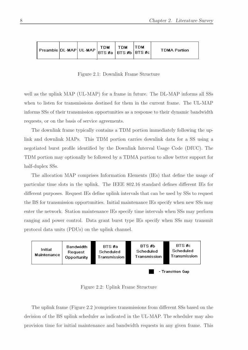
8 Chapter 2. Literature Survey
Figure 2.1: Downlink Frame Structure
well as the uplink MAP (UL-MAP) for a frame in future. The DL-MAP informs all SSs
when to listen for transmissions destined for them in the current frame. The UL-MAP
informs SSs of their transmission opportunities as a response to their dynamic bandwidth
requests, or on the basis of service agreements.
The downlink frame typically contains a TDM portion immediately following the up-
link and downlink MAPs. This TDM portion carries downlink data for a SS using a
negotiated burst profile identified by the Downlink Interval Usage Code (DIUC). The
TDM portion may optionally be followed by a TDMA portion to allow better support for
half-duplex SSs.
The allocation MAP comprises Information Elements (IEs) that define the usage of
particular time slots in the uplink. The IEEE 802.16 standard defines different IEs for
different purposes. Request IEs define uplink intervals that can be used by SSs to request
the BS for transmission opportunities. Initial maintenance IEs specify when new SSs may
enter the network. Station maintenance IEs specify time intervals when SSs may perform
ranging and power control. Data grant burst type IEs specify when SSs may transmit
protocol data units (PDUs) on the uplink channel.
Figure 2.2: Uplink Frame Structure
The uplink frame (Figure 2.2 )comprises transmissions from different SSs based on the
decision of the BS uplink scheduler as indicated in the UL-MAP. The scheduler may also
provision time for initial maintenance and bandwidth requests in any given frame. This
2.2. Overview of 802.16 9
information is conveyed to the SSs by the corresponding IEs in the UL-MAP. The uplink
frame also contains guard times in the form of SS Transition Gaps. These gaps are used
by the BS to re-synchronise to different SS transmissions.
2.2.2 Physical Layer
The IEEE 802.16 PHY systems operates in the range of 10 to 66 GHz. Line-of-sight
propagation paths are a practical necessity in such systems. The standard specifies single-
carrier modulation schemes with FEC. The air interface supports both FDD and TDD
operation modes.
The standard supports three different modulation schemes. It supports higher order
16-QAM and 64-QAM schemes to maximise link throughput and also supports QPSK
for robustness and reliability. While both QPSK and 16-QAM are mandatory on the
downlink, the uplink need support only QPSK.
2.2.3 Scheduling Service Classes
The IEEE 802.16 MAC defines various scheduling service classes. Subscriber stations can
establish connections using the scheduling service class most suitable for the application
in use. Each SS negotiates its service agreements with the BS during connection setup.
The BS uses these scheduling classes while allocating uplink bandwidth for the SSs. The
scheduling service classes defined in IEEE 802.16 are Unsolicited Grant Service (USG),
Real-Time Polling Service (rtPS), Non-Real-Time Polling Service (nrtPS), and Best Effort
(BE) Service.
USG pre-allocates periodic transmission opportunities to the SSs. This eliminates
the overhead involved in the bandwidth request-grant process. The grant size is a sys-
tem parameter negotiated at connection setup and is a part of the service agreements.
Real-Time Polling Service ensures that SSs get periodic bandwidth request opportuni-
ties. The SSs can then request bandwidth from the BS. This service permits the SSs
to transmit without contending for the uplink channel and is ideal for applications that
periodically generate variable sized packets. It targets applications such as voice over
Internet Protocol (VoIP),streaming audio and streaming video. Non-Real-Time Polling
Service is designed for applications that need high bandwidth connections and are not

10 Chapter 2. Literature Survey
delay sensitive, for example, bulk file transfers. Best Effort service targets best effort
traffic where no throughput or delay guarantees are necessary. Here, the SSs are required
to contend for transmission opportunities. The availability of contention opportunities
is not guaranteed. The IEEE 802.16 MAC also provides support for fragmentation and
concatenation.
2.2.4 Radio Link Control
In addition to performing the traditional functions, such as power control and ranging, the
RLC is responsible for transitioning from one PHY scheme to another. Combinations of
PHY modulation and FEC schemes used between the BS and SSs are termed as downlink
or uplink burst profiles depending on the direction of flow. In IEEE 802.16, burst profiles
are identified using Downlink Interval Usage Code (DIUC) and Uplink Interval Usage
Code (UIUC). The RLC is capable of switching between different PHY burst profiles on a
per-frame and per-SS basis. The SSs use preset downlink burst proles during connection
setup.Thereafter, the BS and the SSs continuously negotiate uplink and downlink burst
profiles in an effort to optimise network performance.
2.3 WiFiRe MAC design
The WiFiRe MAC layer is designed for use with directional antennas for enhancing the
reach of 802.11b PHY in rural scenario. The radiation patterns of directional antennas
for a transmitter gives rise to sectorized coverage areas as depicted in figure 2.3. Typically
multiple sectorized antennas are required to cover an area that an omni-directional would
have covered otherwise. System uses multiple sectorized antennas not only for longer
reach but also for complete coverage around transmitting point/tower. As a result, the
MAC layer is a multi-sector MAC requiring a functionality that can control all antennas
simultaneously.
All the sectors in a multiple antenna configuration continue to use the same frequency
channel. As a result, transmission by one antenna will interfere with that of an adjacent
sector. On the other hand, depending on antenna models and transmission power level,
opposite sectors may be completely free from interference with respect to each other. In
any case, in order to avoid interference conflicts, the MAC layer needs to co-ordinate the

2.4. Related Literature 11
Figure 2.3: A Multi-Sector MAC controlling multiple sector
transmission between the antennas.
In a multi-sector system, each antenna is controlled by an 802.11b PHY. The MAC
layer sits on top of all of these 802.11b PHY(s). From the perspective of the MAC, each
PHY (hence each BS antenna) is addressable and identifiable. Thus a single MAC con-
trols more than one PHY and is responsible for scheduling MAC messages appropriately,
while resolving possible transmission conflict from the perspective of receivers. The MAC
layer uses TDD in uplink and down link directions to avoid conflict between interfering
antennas.
This aspect of sectorization of coverage area while using the same frequency channel
for all the sector antennas is a key feature of the system. It not only impacts the design
of the MAC protocol between transmitter and receiver(s) but also the scheduling policies
and the system performance.
2.4 Related Literature
[3] Discusses various issues in using 802.11 family of wireless technologies for long distance
transmission in rural environment, such as quality of 802.11 PHY performance outdoors,

12 Chapter 2. Literature Survey
range extension, spectral vs. cost efficiency, cost of building towers. It gives the details of
the 802.11 based mesh networks deployed in the Digital Gangetic Plains Project providing
voice and data service to villages. [4] and [5] discusses the issues in using CSMA/CA in
networks including long distance links. CSMA/CA is designed to resolve contention in
indoor environment. It is inefficient in long distance point-to-point links, They designed
a new MAC for mesh networks synTX/synRX, which in the context of our problem
translates to saying that the antennas at the base station should be either all be in
transmit mode or all in the receive mode and the transmissions should satisfy some power
relations.
Deploying long distance 802.11 mesh network is not scalable.
• As the number of nodes increase the number of antennas at the BS also increases.
• With too many hops reliability is problem.
[6] Talks about how the inexplicitly specified parameters of 802.11 can be exploited to
increase the range up to 6 Km. But it doesn’t achieve a good throughput.
In next chapter we will give brief introduction to OPNET simulator.

Chapter 3
Choice of Simulator
3.1 QualNet
Initially we started with QualNet[7] since partial implementation of WiMAX was available
in QualNet [8]. But the implementation was for Base Station with one omni-directional
antenna. QualNet specification says that it has support for directional antennas. The
antenna pattern has to be specified in three dimension(3D) using angle θ (theta) and
angle φ (phi) as follows shown in figure 3.1
Figure 3.1: Describing antenna pattern using Φ and Θ
Here φ varies from 0o to 180o and θ varies from 0o to 360o degree. For each value of
φ there are 360 values of θ. These values has to be specified in an ASCII file. Specifying
antenna pattern in QualNet is tedious. QualNet provides directional antenna support
13

14 Chapter 3. Choice of Simulator
only at the receiver end not at transmitter.At transmitter QualNet supports only Omni-
directional antennas.
3.2 OPNET
3.2.1 We chose OPNET because
• OPNET[9] provides directional antenna support both at transmitter and receiver.
• It provides graphical editor for creating antenna patterns
• In November OPNET released the WiMAX(MAC) patch,which we could refer to
for our implementation.
3.3 OPNET Overview
3.3.1 Pipeline Stages in OPNET
Since wireless is basically a broadcast medium, a single transmission can affect many re-
ceivers simultaneously. Received signal strength at each receiver depends on many factors
such as transmitted signal power, distance between transmitter and receiver environment
noise etc. So each receiver may receive the transmitted signal differently. The timing of
signal reaching the receivers also varies. Hence separate pipeline must be executed for
each eligible receiver.
The radio transceiver pipeline consist of total fourteen stages most of which must be exe-
cuted on per receiver basis. All of the pipeline stages can be modified. Below is description
of each stage :
1. Receiver Group
Each transmitter maintains its own list of receiver group which are possible candi-
dates of receiving transmission from the object. The purpose is to create an initial
receiver group for each transmitter channel. The kernel evaluates each receiver
against the transmitter in order to create the receiver group for the transmitter
channel.
3.3. OPNET Overview 15
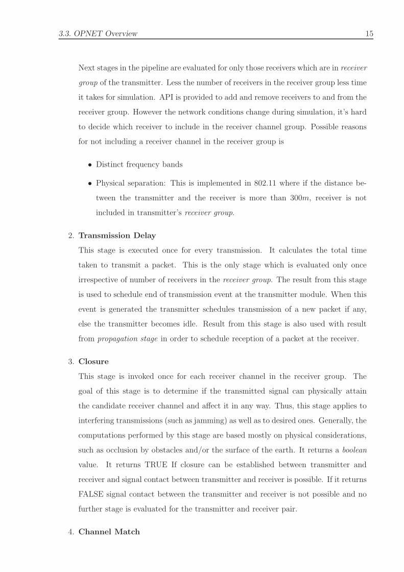
Next stages in the pipeline are evaluated for only those receivers which are in receiver
group of the transmitter. Less the number of receivers in the receiver group less time
it takes for simulation. API is provided to add and remove receivers to and from the
receiver group. However the network conditions change during simulation, it’s hard
to decide which receiver to include in the receiver channel group. Possible reasons
for not including a receiver channel in the receiver group is
• Distinct frequency bands
• Physical separation: This is implemented in 802.11 where if the distance be-
tween the transmitter and the receiver is more than 300m, receiver is not
included in transmitter’s receiver group.
2. Transmission Delay
This stage is executed once for every transmission. It calculates the total time
taken to transmit a packet. This is the only stage which is evaluated only once
irrespective of number of receivers in the receiver group. The result from this stage
is used to schedule end of transmission event at the transmitter module. When this
event is generated the transmitter schedules transmission of a new packet if any,
else the transmitter becomes idle. Result from this stage is also used with result
from propagation stage in order to schedule reception of a packet at the receiver.
3. Closure
This stage is invoked once for each receiver channel in the receiver group. The
goal of this stage is to determine if the transmitted signal can physically attain
the candidate receiver channel and affect it in any way. Thus, this stage applies to
interfering transmissions (such as jamming) as well as to desired ones. Generally, the
computations performed by this stage are based mostly on physical considerations,
such as occlusion by obstacles and/or the surface of the earth. It returns a boolean
value. It returns TRUE If closure can be established between transmitter and
receiver and signal contact between transmitter and receiver is possible. If it returns
FALSE signal contact between the transmitter and receiver is not possible and no
further stage is evaluated for the transmitter and receiver pair.
4. Channel Match

16 Chapter 3. Choice of Simulator
This stage is invoked for every receiver channel that satisfies the link closure stage.
The purpose of this stage is to classify the current transmission for a particular
receiver channel as follows:
• Valid Transmissions in this category are considered compatible with the re-
ceiver channel. The packet may be accepted and forwarded to next modules
for further processing.
• Noise : In this class the data can not be received at the receiver but the
transmission can generate the interference at the receiver.
• Ignore Transmissions in this class does not affect the receiver channel in any
way and hence can be ignored. Further pipeline stages are suspended for the
current transmission.
5. Transmitter Antenna Gain
This is the fifth stage of the transceiver pipeline. Transmission antenna gain is cal-
culated for all receivers that are classified noise or valid by the channel match stage.
It is calculated using the vector between the transmitter and receiver. Transmitter
antenna gain calculated by this stage is used by power model.
6. Propagation Delay Propagation Delay is the time taken bay the packet signal to
travel from source to destination. It depends on the distance between the transmitter
and receiver. propagation delay is calculated for every receiver that is classified noise
or valid by the channel match stage. propagation delay with transmission delay is
used to schedule the packet arrival event at the receiver.
7. Receiver Antenna Gain
This is first stage at the receiver and seventh stage of the pipeline. receiver antenna
gain is calculated at each receiver depending on the vector leading from receiver to
transmitter. This is used in calculation of received power in power model.
8. Receiver Power
Received Power is calculated for each eligible destination channel at the receiver.
The purpose of this stage is to calculate the received power of arriving packet’s
signal (in watts). For the packets that are classified as valid, the received power is
an indication of how accurately receiver can capture the information in packet. The
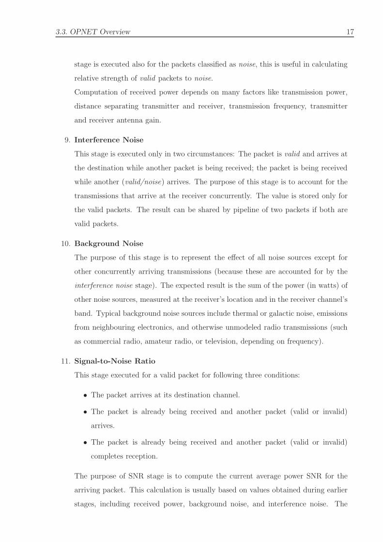
3.3. OPNET Overview 17
stage is executed also for the packets classified as noise, this is useful in calculating
relative strength of valid packets to noise.
Computation of received power depends on many factors like transmission power,
distance separating transmitter and receiver, transmission frequency, transmitter
and receiver antenna gain.
9. Interference Noise
This stage is executed only in two circumstances: The packet is valid and arrives at
the destination while another packet is being received; the packet is being received
while another (valid/noise) arrives. The purpose of this stage is to account for the
transmissions that arrive at the receiver concurrently. The value is stored only for
the valid packets. The result can be shared by pipeline of two packets if both are
valid packets.
10. Background Noise
The purpose of this stage is to represent the effect of all noise sources except for
other concurrently arriving transmissions (because these are accounted for by the
interference noise stage). The expected result is the sum of the power (in watts) of
other noise sources, measured at the receiver’s location and in the receiver channel’s
band. Typical background noise sources include thermal or galactic noise, emissions
from neighbouring electronics, and otherwise unmodeled radio transmissions (such
as commercial radio, amateur radio, or television, depending on frequency).
11. Signal-to-Noise Ratio
This stage executed for a valid packet for following three conditions:
• The packet arrives at its destination channel.
• The packet is already being received and another packet (valid or invalid)
arrives.
• The packet is already being received and another packet (valid or invalid)
completes reception.
The purpose of SNR stage is to compute the current average power SNR for the
arriving packet. This calculation is usually based on values obtained during earlier
stages, including received power, background noise, and interference noise. The

18 Chapter 3. Choice of Simulator
SNR of the packet is important in determining receiver’s ability to correctly receive
the packet’s content. The result computed by this stage is used by the Kernel to
update standard output results of receiver channels and usually also by later stages
of the pipeline.
12. Bit Error Rate
BER stage is executed for all the valid packets for which SNR stage is executed.
The purpose of the BER stage is to derive the probability of bit errors during the
past interval of constant SNR. This is not the empirical rate of bit errors, but the
expected rate, usually based on the SNR. In general, the bit error rate provided
by this stage is also a function of the type of modulation used for the transmitted
signal.
13. Error Allocation
The purpose of the error allocation stage is to estimate the number of bit errors in a
packet segment where the bit error probability has been calculated and is constant.
This segment might be the entire packet, if no changes in bit error probability occur
over the course of the packet’s reception. Bit error count estimation is usually based
on the bit error probability (obtained from stage 11) and the length of the affected
segment.
14. Error Collection
Error correction stage is invoked when a packet completes reception. This stage
determines acceptance of packet. This is usually dependent upon whether the packet
has experienced collisions or not, this result computed in the error allocation stage,
and the ability of the receiver to correct the errors affecting the packet (hence the
name of the stage). Based on the determination of this stage, the Kernel will either
destroy the packet, or allow it to proceed into the destination node. In addition,
this result affects error and throughput results collected for the receiver channel.

Chapter 4
Modelling WiFiRe in OPNET
4.1 Overview of Model in OPNET
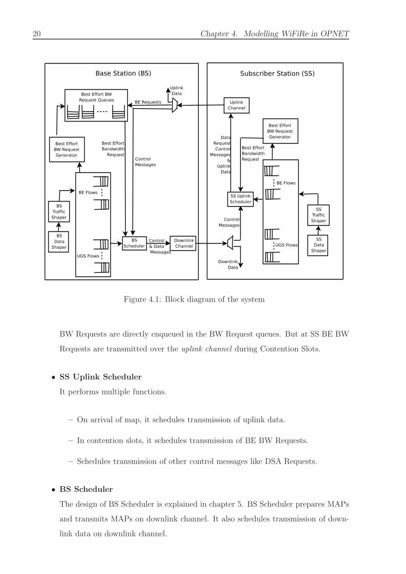
Figure 4.1 shows the block diagram of the System. It consists of two parts, Base Station
(BS) and the Subscriber Station (SS). The BS consists of BS data classifier, BS traffic
shaper, Packet queues, BS Scheduler, BE Bandwidth request generator, and Bandwidth
request queues. The SS consists of SS data classifier, SS traffic shaper, Packet queues,
BE Bandwidth request generator, and SS uplink scheduler.
WiFiRe is a connection oriented MAC. Each incoming packet is mapped to a connec-
tion, which is indexed by Connection Identifier (CID). The packet enters the MAC at the
classifier(BS Data Classifier or SS Data Classifier). The classifier directs the packets from
the higher layer to one of the outgoing connections. Different classifiers can be defined at
each node.
The packets received from the Uplink Channel can be either Data packets, Best Effort
Bandwidth (BE BW) Request packets, or Control packets. The Data packets are sent to
the upper layers for further processing. The BE BW request packets are queued according
to the CID of the connection in the BE BW request queues. Control packets are passed
to the BS Scheduler.
The packets received from the Downlink Channel can be either Data packets or Control
packets. The data packets are sent to the upper layers for further processing. The control
packets are either MAPs or Dynamic Service Addition (DSA) response messages. The
control packets are sent to the SS Uplink Scheduler for further processing.
• BE BW Request Generator
It generates BW request for BE flow, if BE queue has packets to send. At BS, BE
19
20 Chapter 4. Modelling WiFiRe in OPNET
Figure 4.1: Block diagram of the system
BW Requests are directly enqueued in the BW Request queues. But at SS BE BW
Requests are transmitted over the uplink channel during Contention Slots.
• SS Uplink Scheduler
It performs multiple functions.
– On arrival of map, it schedules transmission of uplink data.
– In contention slots, it schedules transmission of BE BW Requests.
– Schedules transmission of other control messages like DSA Requests.
• BS Scheduler
The design of BS Scheduler is explained in chapter 5. BS Scheduler prepares MAPs
and transmits MAPs on downlink channel. It also schedules transmission of down-
link data on downlink channel.

4.2. Assumptions 21
4.2 Assumptions
In the implementation of current model, following assumptions are made.
1. All the SS and BS start at the same time. No ranging is performed. BS after
becoming ready, starts transmitting MAPs. Each SS receives the MAPs and, it
associates with the BS antenna from which it receives maximum power. Each SS
informs BS about the BS antenna if it is associated with and sends the interference
matrix to BS which is used by scheduler.
2. The structure of DSA messages is defined but, DSA messages are exchanged before
the simulation starts.
3. DSC messages are not supported.
4.3 MAC State Diagrams
Figure 4.2 shows the state diagram of the MAC. It shows the states that are common to
both BS and SS. The description of each state is given below in pseudo C code.
In Init state all variables are initialised. MAC and IP addresses are obtained.
A given node can be either a SS or BS. BS ROLE defines whether a given node is
SS or BS. Depending on value of BS ROLE corresponding process is invoked. When a
process is invoked, the control is passed to the invoked process. The invoked process is
termed as child of the process that invoked it. Control returns to the parent process once
the child gets blocked.
Listing 4.1: Invoke Corresponding Process� �
/∗∗∗∗∗∗∗∗∗∗ Invoke correspond ing process ∗∗∗∗∗∗∗∗∗∗/
//BS ROLE i s TRUE i f the node i s a Base S ta t i on .
i f (BS ROLE == TRUE)
invoke ( b s con t r o l )
else
invoke ( s s c o n t o l )

22 Chapter 4. Modelling WiFiRe in OPNET
Figure 4.2: MAC State Diagram
System then enters the Ready state and waits for the events.
When MAC receives packet from higher layer, it makes transition to Enqueue state.
Each incoming higher layer packet is mapped to one of outgoing connection, identified
by a CID. A CID has a queue associated with it. The packet which does not match any
condition specified in classifier is inserted in default BE connection queue.
Listing 4.2: Enqueue� �
/∗∗∗∗∗∗∗∗∗∗Enqueue ∗∗∗∗∗∗∗∗∗∗/
// packe t contains , packe t r e c e i v e d from h ighe r l a y e r
c id = c l a s s i f y p a c k e t ( packet )
/∗INVALID( c id ) re turns TRUE i f c i d i s NULL, e l s e i t
r e turns FALSE∗/
i f (INVALID( c id ) )

4.3. MAC State Diagrams 23
i n s e r t p a c k e t ( de fau l t queue , packet )
else
queue = get queue ( c id )
i n s e r t p a c k e t ( queue , packet )
When control packet arrives from the lower layer, child process is invoked and the
packet is passed to child process. Control returns to the parent process once the child
gets blocked.
Listing 4.3: Process Control Packet� �
/∗∗∗∗∗∗∗∗∗∗Process Contro l Packet ∗∗∗∗∗∗∗∗∗∗/
// con t r o l packe t s are processed by BS and SS proce s s e s
i f (BS ROLE == TRUE)
pass packet ( b s con t r o l )
else
pass packet ( s s c o n t o l )
MAP is processed in similar way at both BS and SS. When MAP arrives, node checks
each map element in the map. If the CID in map element belongs to node, the information
in map element is used to schedule transmission by the node. The map element contains
following fields.
• CID
• Start Slot (Slot number at which transmission should start)
• Number of Slots (Number of slots alloted for transmission)
Listing 4.4: Process Map� �
/∗∗∗∗∗∗∗∗∗∗Process Map∗∗∗∗∗∗∗∗∗∗∗/
for each map element
c id = g e t c i d ( map element )
// e x i s t s ( c i d ) re turns TRUE i f c i d be l ong s to the

24 Chapter 4. Modelling WiFiRe in OPNET
// current node .
i f ( ! e x i s t s ( c id ) )
next
// ge t the packe t queue correspond ing to the c i d
queue = get queue ( c id )
s l o t s a l l o c a t e d = g e t s l o t s ( map element )
do
head pk s i z e = g e t pk s i z e ( queue , 1) ;
i f ( s l o t s a l l o c a t e d < ( head pk s i z e + TX OVERHEAD)
break ;
packet = remove pk ( queue , 1 )
schedule pk ( packet )
s l o t s a l l o c a t e d −= ( head pk s i z e + TX OVERHEAD)
while ( 1 )
i f ( s l o t s a l l o c a t t e d > MIN TX QUANTITY)
packet =remove pk part ( queue , 1 , s l o t s a l l o c a t e d −
TX OVERHEAD)
schedu l e pk par t ( packet )
When MAC receives data packet form PHY, it is passed to the higher layer for further
processing.
Listing 4.5: Process Data Packet� �
/∗∗∗∗∗∗∗∗∗∗Process Data Packet ∗∗∗∗∗∗∗∗∗∗/
g e t i p p a ck e t s ( packet )
{
while ( ip pk = get packe t ( packet ) )
i f (COMPLETE( ip pk ) )
s end pk to uppe r l a y e r ( ip pk )
else

4.4. Base Station State Diagram 25
compl pk = in s e r t pa cke t s e g queue (q , packet )
/∗ i f i n s e r t i n g the packe t segement in q forms
a complete packe t then i n s e r t p a c k e t s e g q u e u e
re turns the packe t . E l se re turns NIL∗/
i f ( compl pk != NIL)
s end pk to uppe r l a y e r ( compl pk )
}
c id = g e t c i d ( packet )
i f (INVALID( c id ) )
drop packet ( packet )
e x i t
g e t i p p a ck e t s ( packet )
4.4 Base Station State Diagram
Figure 4.3 shows the state diagram of a BS. The description of states is given below in
pseudo C code.
Init state initialises all the variables specific to BS. It also places(directs) the antennas
(six in current implementation) at the BS.
Listing 4.6: Init State� �
/∗∗∗∗∗∗∗∗∗∗ I n i t ∗∗∗∗∗∗∗∗∗∗/
i n i t i a l i z e v a r i a b l e s ( ) // I n i t i a l i z e s a l l the v a r i a b l e s
p la ce antennas ( ) ; // p l ace a l l the antennas
The BW Request is inserted in BE BW Request queue, identified by CID.
Listing 4.7: Process BW Request� �
/∗∗∗∗∗∗∗∗∗∗BW Request Process ∗∗∗∗∗∗∗∗∗∗/
//BW reque s t s come only from the BE f l ow s

26 Chapter 4. Modelling WiFiRe in OPNET
Figure 4.3: State Diagram of Base Station)
c id = g e t c i d ( packet )
i f ( ! e x i s t s ( c id ) )
e x i t
//enque bw re que s t in a queue
queue = get queue ( c id )
enqueue ( queue , bw req )
Listing 4.8: Process DSA Request� �
/∗∗∗∗∗∗∗∗∗∗DSA Request Process ∗∗∗∗∗∗∗∗∗∗/
// t o t a l s l o t s p e r f r am e i s t o t a l number o f s l o t s in a

4.4. Base Station State Diagram 27
frame
/∗ t o t a l s l o t s p e r f r am e f r e e i s t o t a l number o f s l o t s in
frame
f r e e cu r r en t l y ∗/
// da ta ra t e i s d a t a ra t e o f the channe l
s e r v i c e f l ow t yp e = ge t s e r v i c e f l ow t yp e ( packet )
s e r v i c e f l ow d i r e c t i o n = ge t s e r v i c e f l ow d i r e c t i o n (
packet )
i f ( s e r v i c e f l ow t yp e = = BEST EFFORT)
c id = gene r a t e c i d ( c id )
i f ( s e r v i c e f l ow d i r e c t i o n == DOWNLINK)
cr ea t e queue ( c id )
// c r e a t e s a queue which can be accessed us ing the
c i d
else
s end dsp re sp ( true , c id )
i f ( s e r v i c e f l ow t yp e = = UGS)
bw request = ge t da t a r a t e ( packet )
// ( bw reque s t i s in b y t e s / sec )
avg sdu s i z e = g e t a vg sdu s i z e ( packet )
bw request = bw request + TX OVERHEAD BYTES ∗
avg sdu s i z e
bw request = c o n v e t i n t o s l o t s ( bw request )
bw request per f rame = bw request /
t o t a l s l o t s p e r f r ame
∗ data ra t e
// admi t f l ow () i s f unc t i on o f admission con t r o l .
i f ( admit f low ( bw request per f rame ) )
//admit the f l ow
c id = gene r a t e c i d ( c id ) ;
i f ( s e r v i c e f l o w d i r e c t i o n = = DOWNLINK)
cr ea t e queue ( c id )

28 Chapter 4. Modelling WiFiRe in OPNET
else
s end dsp re sp ( true , c id ) ;
else
s end dsp re sp ( f a l s e .−1) ;
On arrival of Interference Matrix at BS, Association Matrix, Interference Matrix and
Conditional matrix are updated at the BS. The definition of Interference Matrix, Associ-
ation Matrix and Conditional Matrix is given in chapter 5
Listing 4.9: Process Interference Matrix� �
/∗∗∗∗∗∗∗∗∗∗Process I n t e r f e r en c e Matrix ∗∗∗∗∗∗∗∗∗∗/
c a l c u l a t e a s s o c i a t i o n ma t r i x ( )
c a l c u l a t e i n t e r f e r e n c e ma t r i x ( )
c a l c u l a t e c o nd i t i o n a l ma t i x ( )
At end of each frame BS sends MAP, and schedules transmission of next MAP.
Listing 4.10: Send Map� �
/∗∗∗∗∗∗∗∗∗∗Send MAP∗∗∗∗∗∗∗∗∗∗/
map = create map ( ) ;
send map (map)
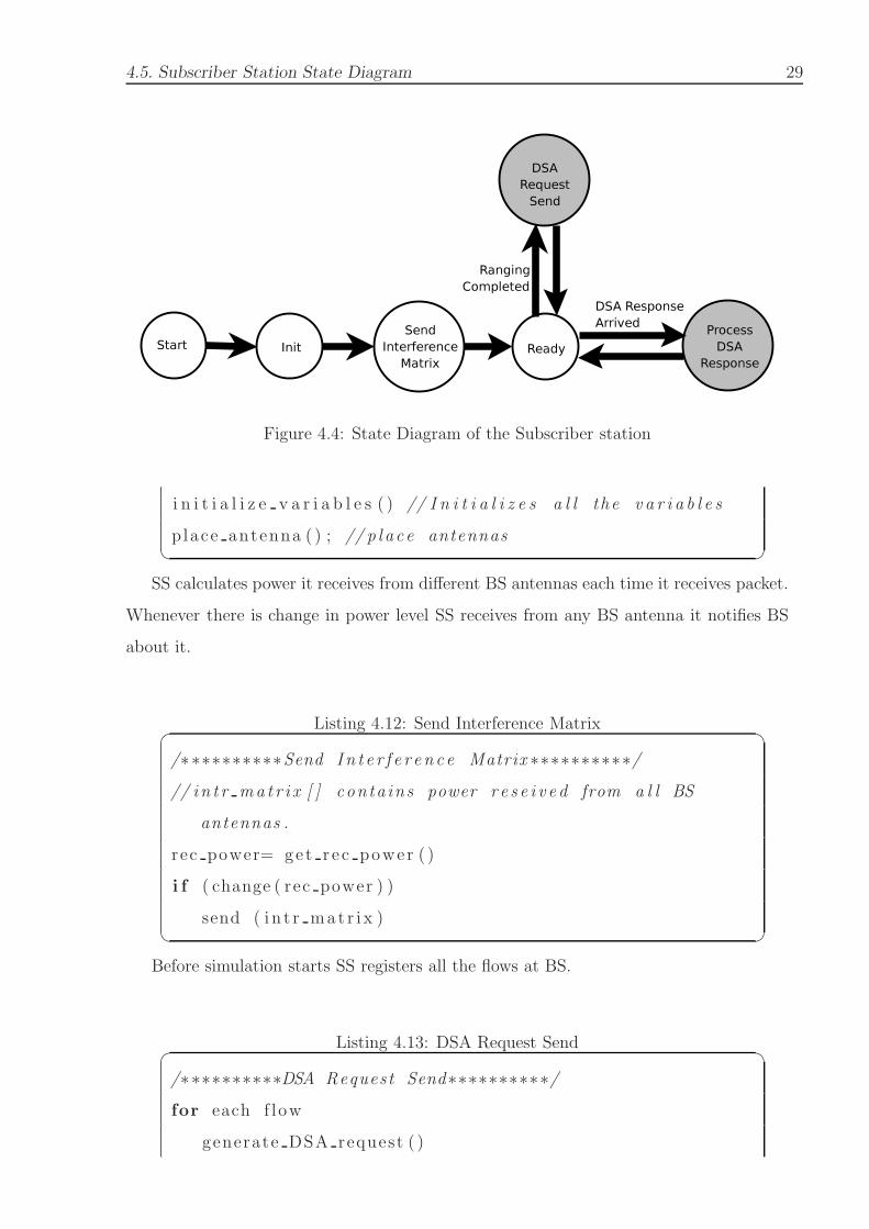
4.5 Subscriber Station State Diagram
SS is simple as compared to BS. Figure 4.4 shows the state diagram of a SS. The descrip-
tion of states is given below in pseudo C code.
When SS is invoked it initialises all variables typical to SS. It also directs the antenna
towards the BS.
Listing 4.11: Init State� �
/∗∗∗∗∗∗∗∗∗∗ I n i t ∗∗∗∗∗∗∗∗∗∗/
4.5. Subscriber Station State Diagram 29
Figure 4.4: State Diagram of the Subscriber station
i n i t i a l i z e v a r i a b l e s ( ) // I n i t i a l i z e s a l l the v a r i a b l e s
place antenna ( ) ; // p l ace antennas
SS calculates power it receives from different BS antennas each time it receives packet.
Whenever there is change in power level SS receives from any BS antenna it notifies BS
about it.
Listing 4.12: Send Interference Matrix� �
/∗∗∗∗∗∗∗∗∗∗Send In t e r f e r en c e Matrix ∗∗∗∗∗∗∗∗∗∗/
// in t r ma t r i x [ ] conta ins power r e s e i v e d from a l l BS
antennas .
rec power= get r ec power ( )
i f ( change ( rec power ) )
send ( i n t r ma t r i x )
Before simulation starts SS registers all the flows at BS.
Listing 4.13: DSA Request Send� �
/∗∗∗∗∗∗∗∗∗∗DSA Request Send∗∗∗∗∗∗∗∗∗∗/
for each f low
generate DSA request ( )

30 Chapter 4. Modelling WiFiRe in OPNET
send DSA request ( )
Listing 4.14: Process DSA Response� �
/∗∗∗∗∗∗∗∗∗∗DSA Response process ∗∗∗∗∗∗∗∗∗∗/
response g e t r e rpon s e ( packet )
i f ( response == TRUE)
cr ea t e queue ( c id )
Next chapter discusses the design of Scheduler at the BS.
Chapter 5
Scheduler
In order to test the model implementation and the performance, we need to also implement
scheduler at the BS. We have implemented Greedy Heuristic Scheduler [1].
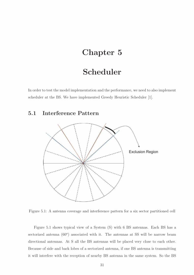
5.1 Interference Pattern
Figure 5.1: A antenna coverage and interference pattern for a six sector partitioned cell
Figure 5.1 shows typical view of a System (S) with 6 BS antennas. Each BS has a
sectorized antenna (60o) associated with it. The antennas at SS will be narrow beam
directional antennas. At S all the BS antennas will be placed very close to each other.
Because of side and back lobes of a sectorized antenna, if one BS antenna is transmitting
it will interfere with the reception of nearby BS antenna in the same system. So the BS
31

32 Chapter 5. Scheduler
antennas at System S are either all transmitting or all receiving. The region covered by
solid (red) lines shows the communication range of the BS antenna and forms the sector
of the BS antenna. The region covered by dotted (blue) lines on either side of the sector
shows the exclusion (taboo) region of the antenna. All the SSs in a sector will associate
with the antenna serving that sector. Depending on interference The transmission in one
sector may prohibit transmission between some BS-SS pairs in the nearby sector.
5.2 Greedy Heuristic Scheduler [1]
5.2.1 Notation and Terminology
• number of BS antennas at S (n):. For the setup we are using, the number of BS
antennas are 6. This number varies depending on density of SSs in the region.
Increasing the number of BS antennas at S increases the capacity of system up to a
limit.
• number of SSs (m) : The number of SS in a sector j is denoted by mj and number
of SSs in exclusion region in clockwise previous sector by mj− .Similarly we define
mj+.
• Association Matrix (A): Association matrix is an m x n matrix where each row
corresponds to a SS and each column corresponds to BS antenna. The (i, j)th
element of the matrix A is 1 if ith SS i is associated with jth BS antenna. SS i is
associated with BS antenna j when power received by i from the packet sent by j
is greater than some specified communication threshold. Otherwise it is 0
• Exclusion Matrix (I): Exclusion matrix is a m x n matrix, where m is number of
SS and n is number of BS antennas. The (i, j)th element of matrix I is 1 if power
received by i from the packet sent by j is greater then some specified interference
threshold . Other wise its 0
• Activation vector(u): Activation vector is a 1 x n matrix where ith element denotes
which SS in sector i is active. All active SSs may be either transmitting or receiving.
• Maximal Activation Vector (U) : If no more SS in an activation vector can be

5.2. Greedy Heuristic Scheduler [1] 33
activated without causing interference to some other transmissions scheduled in the
same vector then this activation vector is maximal.
• Schedule (S): Schedules consist of SSs that are active at any given time.
• Interfering Links ι(S) This is set of SSs that can interfere with the links in S.
• UGS Grants (q) : q is m x 1 matrix. Where each row specifies the UGS grants for
the corresponding SS.
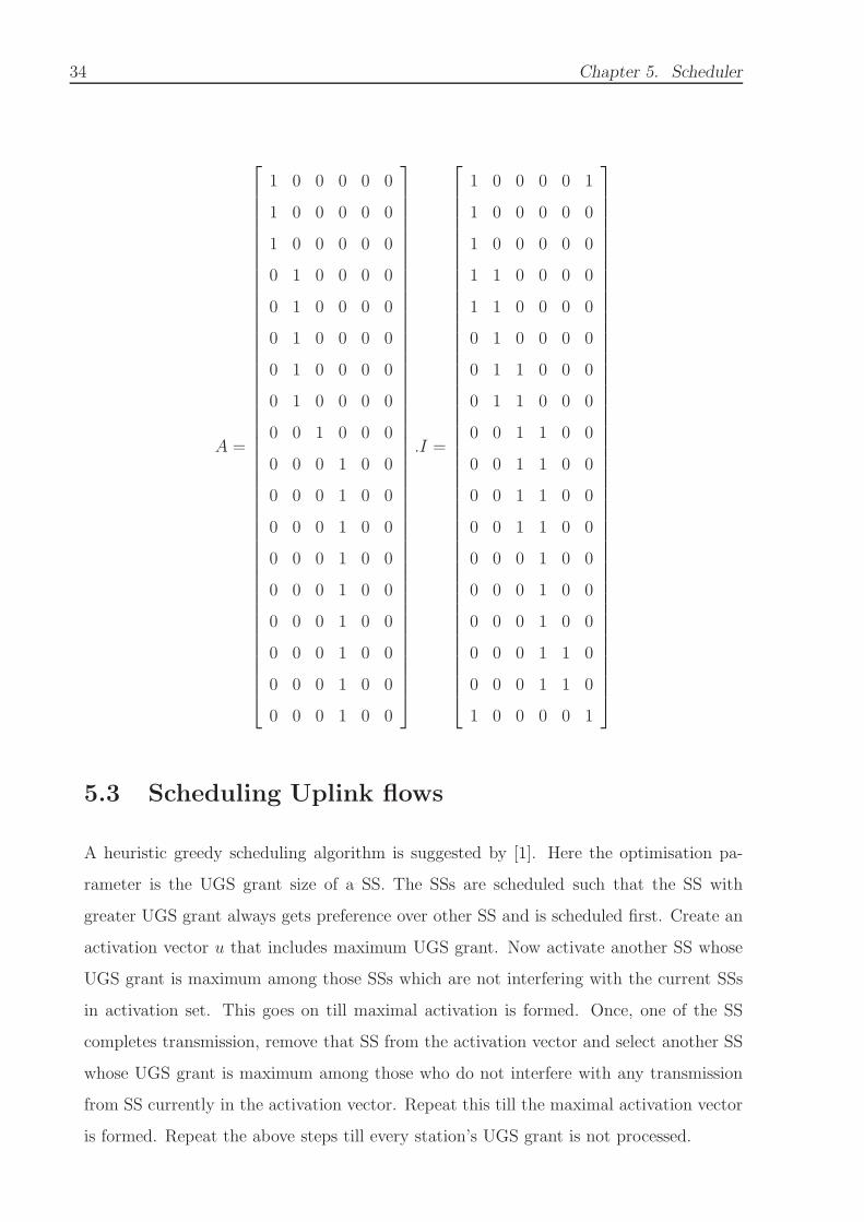
5.2.2 Example
To explain the notations above consider the following example
Figure 5.2: Example scenario of the system
The association matrix A and Interference matrix I for figure 5.2 is:
34 Chapter 5. Scheduler
A =
1 0 0 0 0 0
1 0 0 0 0 0
1 0 0 0 0 0
0 1 0 0 0 0
0 1 0 0 0 0
0 1 0 0 0 0
0 1 0 0 0 0
0 1 0 0 0 0
0 0 1 0 0 0
0 0 0 1 0 0
0 0 0 1 0 0
0 0 0 1 0 0
0 0 0 1 0 0
0 0 0 1 0 0
0 0 0 1 0 0
0 0 0 1 0 0
0 0 0 1 0 0
0 0 0 1 0 0
.I =
1 0 0 0 0 1
1 0 0 0 0 0
1 0 0 0 0 0
1 1 0 0 0 0
1 1 0 0 0 0
0 1 0 0 0 0
0 1 1 0 0 0
0 1 1 0 0 0
0 0 1 1 0 0
0 0 1 1 0 0
0 0 1 1 0 0
0 0 1 1 0 0
0 0 0 1 0 0
0 0 0 1 0 0
0 0 0 1 0 0
0 0 0 1 1 0
0 0 0 1 1 0
1 0 0 0 0 1
5.3 Scheduling Uplink flows
A heuristic greedy scheduling algorithm is suggested by [1]. Here the optimisation pa-
rameter is the UGS grant size of a SS. The SSs are scheduled such that the SS with
greater UGS grant always gets preference over other SS and is scheduled first. Create an
activation vector u that includes maximum UGS grant. Now activate another SS whose
UGS grant is maximum among those SSs which are not interfering with the current SSs
in activation set. This goes on till maximal activation is formed. Once, one of the SS
completes transmission, remove that SS from the activation vector and select another SS
whose UGS grant is maximum among those who do not interfere with any transmission
from SS currently in the activation vector. Repeat this till the maximal activation vector
is formed. Repeat the above steps till every station’s UGS grant is not processed.

5.3. Scheduling Uplink flows 35
Algorithm 1 Greedy Heuristic algorithm for Uplink Scheduling taken from [1]
INPUT m : number of SSs
n :number of BS antennas
Activation Vector A(m,n)
Interference Vector I(m,n)
UGS grant matrix q(m,1)
//q contains UGS request size of all the SSs in slots.
OUTPUT Schedule S
1: Initially, slot index k = 0. Let SS i be such that
qki = maxl=1...m
{qkl}
i.e. The SS with longest UGS grant at the beginning of slot k is i. Create activation
vector u with link i activated. i.e. u = {i}
2: Let SS j be such that
qkj = maxl
{qkl : l ∋ ι(u)}
j is such that it is maximum among interfering SSs. activate j find new ι(u).
3: Let
n = {qkl : minl=1,...,m
(qkl, l ∈ u)}
i.e. n is the minimum number of slots required for the first SS in u to complete its
transmission. Use u in the schedule from kth to (k + 1)th slot.
qk+n,i =
qk,i − n for i ∈ u
qk,i for i ∋ u
and k = K + n. i.e. slot index advances by n, and the queue length for the SSs ate
the begingin of (k + n)thslot is n less
4: At the end of k + nth slot,
u = u − {l : qkl = min(qkl, l ∈ u)}
i.e., remove those SSs that have completed their UGS grants from activation vector.
5: Go back to step 3 and from maximal activation vector including u. Continue above
procedure until all the SSs are not serviced
6: Once UGS grants are serviced we serve the BE flows in similar way.
36 Chapter 5. Scheduler
5.4 Preprocessing
We extend the Greedy Heuristic Scheduling algorithm for faster implementation by do-
ing preprocessing. we group together the nodes, exhibiting similar characteristics. We
represent the group as a single node.
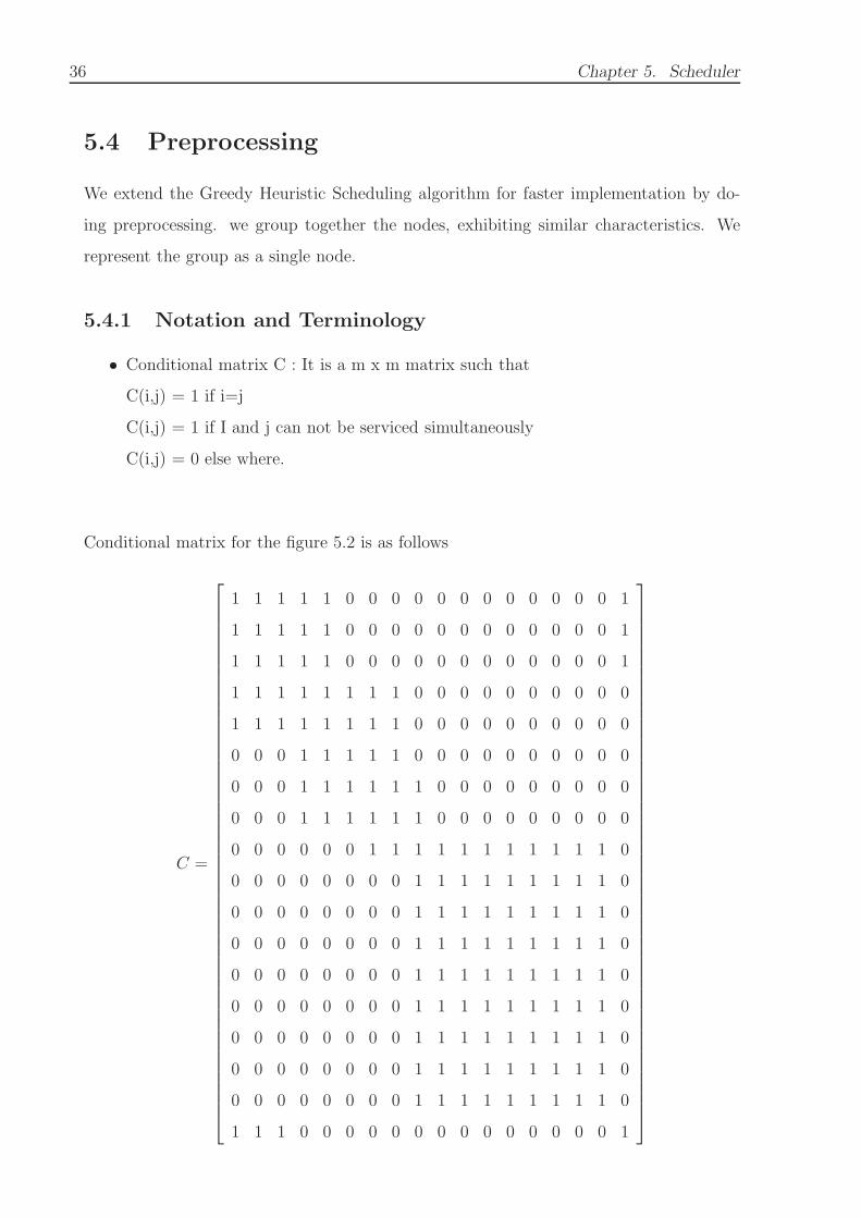
5.4.1 Notation and Terminology
• Conditional matrix C : It is a m x m matrix such that
C(i,j) = 1 if i=j
C(i,j) = 1 if I and j can not be serviced simultaneously
C(i,j) = 0 else where.
Conditional matrix for the figure 5.2 is as follows
C =
1 1 1 1 1 0 0 0 0 0 0 0 0 0 0 0 0 1
1 1 1 1 1 0 0 0 0 0 0 0 0 0 0 0 0 1
1 1 1 1 1 0 0 0 0 0 0 0 0 0 0 0 0 1
1 1 1 1 1 1 1 1 0 0 0 0 0 0 0 0 0 0
1 1 1 1 1 1 1 1 0 0 0 0 0 0 0 0 0 0
0 0 0 1 1 1 1 1 0 0 0 0 0 0 0 0 0 0
0 0 0 1 1 1 1 1 1 0 0 0 0 0 0 0 0 0
0 0 0 1 1 1 1 1 1 0 0 0 0 0 0 0 0 0
0 0 0 0 0 0 1 1 1 1 1 1 1 1 1 1 1 0
0 0 0 0 0 0 0 0 1 1 1 1 1 1 1 1 1 0
0 0 0 0 0 0 0 0 1 1 1 1 1 1 1 1 1 0
0 0 0 0 0 0 0 0 1 1 1 1 1 1 1 1 1 0
0 0 0 0 0 0 0 0 1 1 1 1 1 1 1 1 1 0
0 0 0 0 0 0 0 0 1 1 1 1 1 1 1 1 1 0
0 0 0 0 0 0 0 0 1 1 1 1 1 1 1 1 1 0
0 0 0 0 0 0 0 0 1 1 1 1 1 1 1 1 1 0
0 0 0 0 0 0 0 0 1 1 1 1 1 1 1 1 1 0
1 1 1 0 0 0 0 0 0 0 0 0 0 0 0 0 0 1

5.4. Preprocessing 37
The matrix is symmetric. One can notice that few rows in the matrix are identical. These
rows corresponds to the nodes having similar characteristics like nodes associated with
same antenna, nodes in exclusion region of the same antenna. The idea is to combine
these rows and form new row, which means represent the set of nodes exhibiting similar
characteristics with one node. The UGS grant of this representative node is sum of UGS
grant of all nodes it is representing. In the example given 7 such representative nodes can
be found, as follows
a = {1, 2, 3}
b = {4, 5}
c = {6}
d = {7, 8}
e = {9}
f = {10, 11, 12, 13, 14, 15, 16, 17}
g = {18}
The conditional matrix now reduces to
C =
1 1 0 0 0 0 1
1 1 1 1 0 0 0
0 1 1 1 0 0 0
0 1 1 1 1 0 0
0 0 0 1 1 1 0
0 0 0 0 1 1 0
1 0 0 0 0 0 1
There is not much difference between uplink and downlink scheduling. But in downlink
we can take advantage of the fact that only one station is transmitting. And since it is
a broadcast medium we can combine multiple UGS grants to save PHY overhead. With
the preprocessing that we applied long burst of continuous transmission from the same
BS are possible.
In this chapter we described the design of Scheduler at the BS [1]. We also proposed
an extension to the scheduling algorithm, for faster computation of schedule.
In next chapter we check the validity of the implemented model by performing some
simulation experiments.


Chapter 6
Simulation Setup
6.1 Simulation Setup
Following parameters need to be specified when setting up simulation.
1. Classifier Definition
2. Service Class Definition
3. Packet interarrival time (exponential distribution)
4. Packet size (Uniform Distribution)
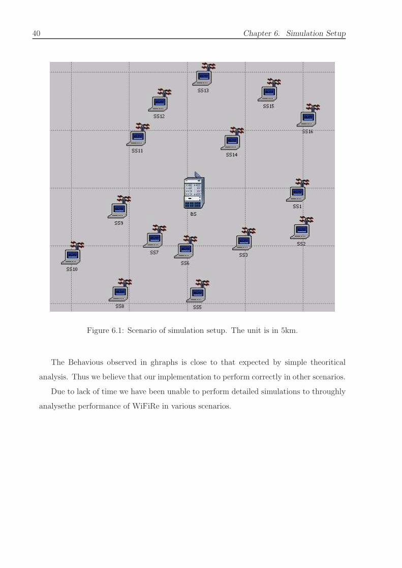
6.2 Scenario
Figure 6.1 shows the scenario of simulation setup. Simulation consist of one BS, sur-
rounded by 16 SS, which are placed randomly around the BS. Each SS has 4 flows reg-
istered at the BS: one UGS downlink flow, one UGS uplink flow, one BE downlink flow
and one BE uplink flow.
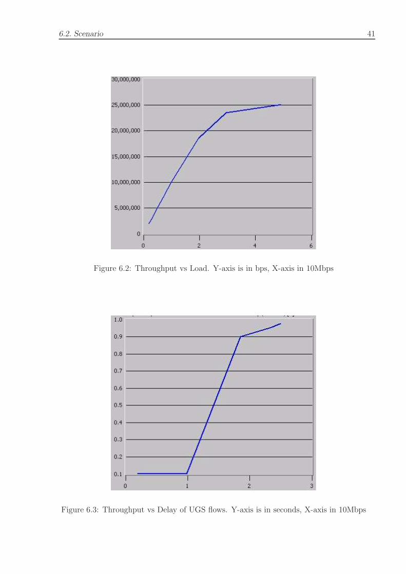
Figure 6.2 shows how throughput of system varies with increasing load. Initially
throughtput of system increases with increase in load. After some load threshold the
throughput reaches the saturation point. For the given scenario achievable throughput is
25 Mbps.
Figure 6.3 shows the delay faced by packets from UGS flows for throughput. The
point upto which UGS flows adhere to the aggreement, delay is less and constant. but
with increase in load beyond a threshold results in longer delayes for UGS flow packets.
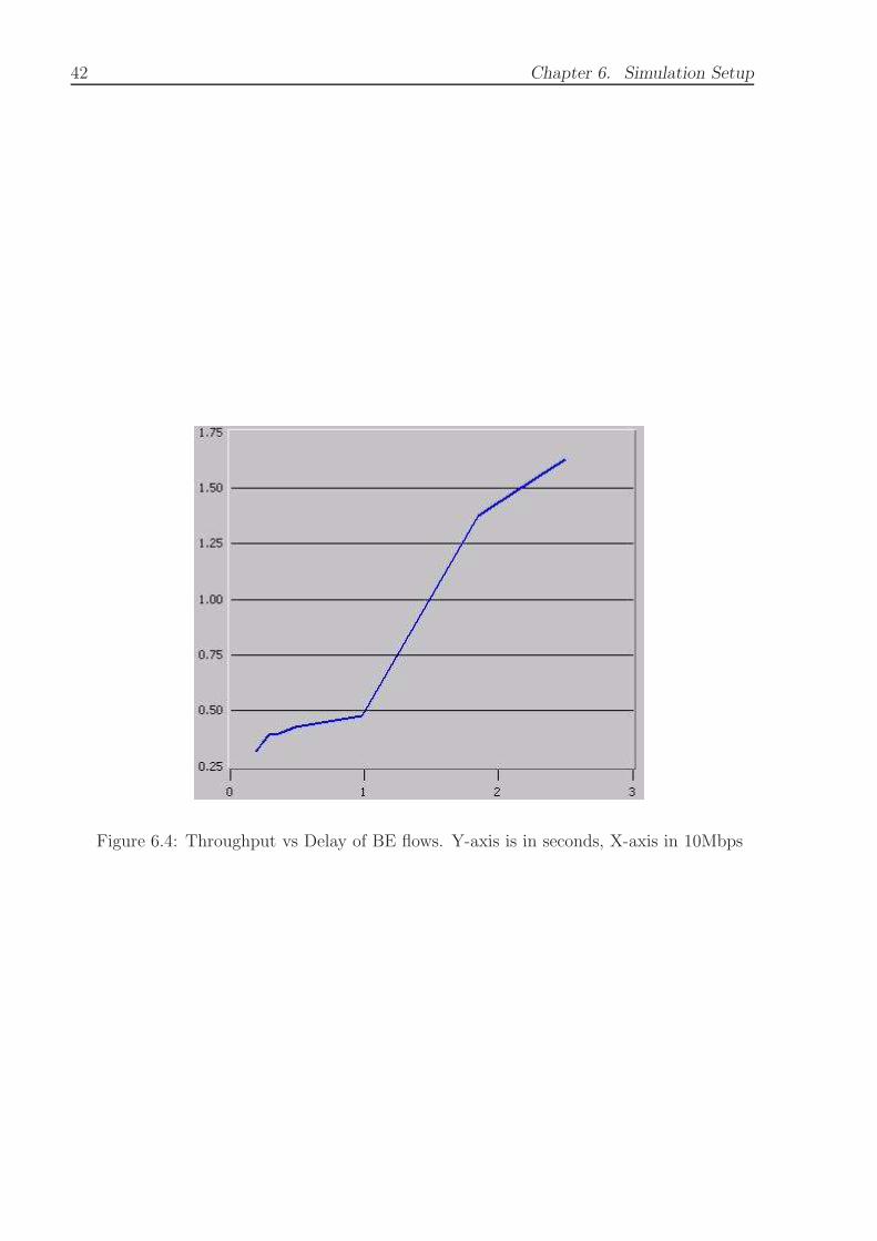
Figure 6.4 shows delay faced by packets from BE flows for given throughput.
39
40 Chapter 6. Simulation Setup
Figure 6.1: Scenario of simulation setup. The unit is in 5km.
The Behavious observed in ghraphs is close to that expected by simple theoritical
analysis. Thus we believe that our implementation to perform correctly in other scenarios.
Due to lack of time we have been unable to perform detailed simulations to throughly
analysethe performance of WiFiRe in various scenarios.
6.2. Scenario 41
Figure 6.2: Throughput vs Load. Y-axis is in bps, X-axis in 10Mbps
Figure 6.3: Throughput vs Delay of UGS flows. Y-axis is in seconds, X-axis in 10Mbps
42 Chapter 6. Simulation Setup
Figure 6.4: Throughput vs Delay of BE flows. Y-axis is in seconds, X-axis in 10Mbps

Chapter 7
Conclusion
We have implemented WiFiRe model in OPNET and checked its correctness by simulation
results. Using WiFiRe we are able estblish communication links over long distance of upto
20 Km with good throughput.
7.1 Future Work
Experiments performed just support the validity of WiFiRe model implemented in OP-
NET. More experiments need to be performed in order to check performance of WiFiRe.
The throughput of system is dependant on the simulation scenario. Maximum achievable
throughput is different in different scenario.
While implementing the WiFiRe model, we relaxed few specifications such as Ranging,
DSC messages etc. These specifications need to be implemented in order to understand
the full functioning of WiFiRe. We also haven’t implemented the extension of Greedy
Heuristic Algorithm.
We believe that most of the code written for opnet model for WiFiRe can be easily
extended for real implementation.
43


Bibliography
[1] Anitha Varghese. Design of a TDD, Single Channel, Multisector TDM MAC for a
Single Cell WiFiRe System. Master’s thesis, ECE Department, IISC Banglore, 2006.
[2] WiFi Rural Extension(WiFiRe), CEWIT Std., 2006.
[3] P. Bhagwat, B. Raman, and D. Sanghi. Turning 802.11 inside-out. ACM SIGCOMM
Computer Communication Review, 34(1):33–38, 2004.
[4] B. Raman and K. Chebrolu. Design and evaluation of a new MAC protocol for
long-distance 802.11 mesh networks. Proceedings of the 11th annual international
conference on Mobile computing and networking, pages 156–169, 2005.
[5] B. Raman and K. Chebrolu. Revisiting MAC Design for an 802.11-based Mesh
Network. Omni, 6(3.0):2.0.
[6] KK Leung, B. McNair, LJ Cimini Jr, and JH Winters. Outdoor IEEE 802.11 cellular
networks: MAC protocol design and performance. Communications, 2002. ICC 2002.
IEEE International Conference on, 1:595–599, 2002.
[7] QualNet Simulator 3.9, 2004. http://www.qualnet.com.
[8] Supriya Maheshwari. An Efficient Qos Scheduling Architecture for IEEE 802.16
Wireless MAN. Master’s thesis, IIT Bombay, 2005.
[9] OPNET Simulator 11.5, 2005. http://www.opnet.com.
[10] OPNET Simulator 11.0, 2005. http://www.opnet.com.
[11] A. Behzad and I. Rubin. On the performance of graph-based scheduling algorithms
for packet radio networks. Global Telecommunications Conference, 2003. GLOBE-
COM’03. IEEE, 6, 2003.
45

Acknowledgements
I take this opportunity to express my sincere gratitude for Prof. Sridhar Iyer for
his constant support and encouragement. His excellent guidance has been instrumental
in making this project work a success.
I would also like to thank my family and friends especially the entire M.Tech.
Batch, who have been a source of encouragement and inspiration throughout the duration
of the project.
Last but not the least, I would like to thank the entire KReSIT family for making my
stay at IIT Bombay a memorable one.
Anirudha Bodhankar
I. I. T. Bombay
July 17th, 2006
47
