Improved Unsteady AerodynamicInfluence Coefficients for Dynamic

Aeroelastic Response

Quinn Murphy

Department of Mechanical EngineeringMcGill UniversityMontreal, Canada

December 2012

A thesis submitted to McGill Universityin partial fulfillment of the requirements for the degree of

Master of Engineering

c©Quinn Murphy 2012

Abstract

Flutter, or the dynamic instability of an aircraft wing due to aerodynamic loads, must be

considered when designing an aircraft. For this reason work has been done to improve a

method developed at Bombardier Aerospace to analyze the dynamic aeroelastic response

of aircraft. This method replaces original Doublet Lattice Method (DLM) aerodynamic

data with that from high-fidelity Computational Fluid Dynamics (CFD) codes. The new

aerodynamic loads are transmitted to the NASTRAN aeroelastic module through improved

Aerodynamic Influence Coefficients (AIC). Previously this high-fidelity data was solely

steady, and weighting factors were needed to obtain unsteady data. This gave good results

for flutter calculations in the subsonic and transonic regime, however, for improved results

in the transonic and supersonic regime, unsteady aerodynamic data was needed. This

research incorporates unsteady high-fidelity CFD data into this analysis method.

The unsteady CFD data was obtained by means of the Transpiration Method. This

allowed for the unsteady movement of the model to be accounted for, while saving compu-

tational time needed to deform and remesh the aerodynamic mesh at each time step. The

transpiration method was validated with two standard test cases, for both static deflections

and unsteady cyclic movement. Once this method was validated, high-fidelity CFD results

could then be used in the AIC method.

The AIC method begins with a set of baseline modes being obtained for the wing

model. From these modes an aerodynamic base is calculated. Using the AIC method

this aerodynamic base is transferred to NASTRAN. The natural mode shapes of a new

configuration, along with the modal-based AIC method are used to approximate aerodynamic

loads for the new configuration. These loads are used in NASTRAN to compute the flutter

analysis of the new configuration.

Resume

Le flottement, ou instabilite dynamique des ailes d’un avion du a sa charge aerodynamique,

doit etre considere lors de la conception d’un avion. Pour cette raison, la methode d’analyse

de l’aeroelasticite d’un avion developpee par Bombardier Aeronautique, doit etre amelioree.

La nouvelle methode, utilisant un code de calcul dynamique des fluides, ou Computational

Fluid Dynamics (CFD), remplace la methode originale du “Doublet Lattice Method”. La

nouvelle charge aerodynamique est transmise au module d’aeroelasticite de NASTRAN a

l’aide d’un “Coefficient d’Influence Aerodynamique (AIC)” ameliore. Precedemment, seules

les donnees stationnaires etaient de haute fidelite et un facteur de correction etait necessaire

pour completer les donnees instationnaires. Ces donnees fournissaient de bons resultats

pour les calculs du flottement en regimes subsonique et transsonique. Cependant, pour les

cas de regimes transsonique et supersonique, des donnees aerodynamiques instationnaires

sont necessaires pour ameliorer les resultats. Cette etude introduit donc les donnees

instationnaires de haute fidelite provenant du calcul dynamique des fluides.

Les donnees instationnaires generees par le calcul dynamique des fluides sont obtenues au

moyen de la “Methode par Transpiration”. Cette methode permet de prendre en compte la

composante instationnaire tout en minimisant le temps de calcul necessaire pour deformer et

remailler le maillage aerodynamique a chaque pas de temps. La methode par Transpiration

a ete valide par deux tests standards, pour des cas de deflections statiques et de mouvements

cycliques instationnaires. Une fois cette methode validee, les resultats de haute fidelite

du calcul dynamique des fluides peuvent etre utilises pour la methode AIC. La methode

AIC est initiee avec des modes de bases obtenus pour des ailes, ce qui permet de calculer

une base aerodynamique. Cette base aerodynamique est ensuite transferee NASTRAN en

utilisant la methode AIC. La forme des modes naturels de la nouvelle configuration, avec

les bases modales de la methode AIC, permet d’approximer la charge aerodynamique de

la nouvelle configuration. Cette charge est ensuite utilisee par NASTRAN pour resoudre

l’analyse du flottement pour la nouvelle configuration.

Acknowledgements

First and foremost, I would like to thank my family, who have supported me throughout

this entire process and my entire career. They have been there for me and are the sole

reason I was able to complete this challenge.

I would also like to thank both of my supervisors, Eddy Zuppel and Prof. Mathias

Legrand, for the support and guidance that they have given to me. This project would not

have been possible without their help.

Finally, I would like to extend my gratitude to everyone in the Controlled Facilities

Engineering Services and Dynamics Groups at Bombardier Aerospace for their continuing

support with this project.

Contents

Introduction 1

1 Literature Review 3

1.1 Current Aeroelastic Analysis . . . . . . . . . . . . . . . . . . . . . . . . . . 3

1.2 Aeroelastic Analysis at Bombardier . . . . . . . . . . . . . . . . . . . . . . . 5

1.2.1 Notations for Matrix Equations . . . . . . . . . . . . . . . . . . . . . 6

1.2.2 Aerodynamic and Structural Data Mapping . . . . . . . . . . . . . . 6

1.2.3 Aerodynamic Loads in NASTRAN . . . . . . . . . . . . . . . . . . . 6

1.2.4 Flutter Solution . . . . . . . . . . . . . . . . . . . . . . . . . . . . . 9

1.3 Unsteady Aerodynamic Analysis . . . . . . . . . . . . . . . . . . . . . . . . 11

1.4 Transonic Aerodynamic Analysis . . . . . . . . . . . . . . . . . . . . . . . . 11

1.5 Modal Based AIC Method . . . . . . . . . . . . . . . . . . . . . . . . . . . . 12

1.6 Transpiration Method . . . . . . . . . . . . . . . . . . . . . . . . . . . . . . 14

1.7 Evaluation of CFD Methods . . . . . . . . . . . . . . . . . . . . . . . . . . . 16

1.7.1 DLM Methodology . . . . . . . . . . . . . . . . . . . . . . . . . . . . 17

1.7.2 Wind Tunnel Methodology . . . . . . . . . . . . . . . . . . . . . . . 17

1.7.3 High-Fidelity CFD Methodology . . . . . . . . . . . . . . . . . . . . 18

i

2 Transpiration Boundary Condition 19

2.1 Undeflected Aerodynamics . . . . . . . . . . . . . . . . . . . . . . . . . . . . 19

2.2 Deflection of the Model . . . . . . . . . . . . . . . . . . . . . . . . . . . . . 20

2.3 Natural Mode Shapes . . . . . . . . . . . . . . . . . . . . . . . . . . . . . . 20

2.4 Defining the Boundary Conditions . . . . . . . . . . . . . . . . . . . . . . . 22

2.5 Computational Fluid Dynamic Simulations . . . . . . . . . . . . . . . . . . 22

2.6 Unsteady Considerations . . . . . . . . . . . . . . . . . . . . . . . . . . . . . 23

2.7 Processing Simulation Results . . . . . . . . . . . . . . . . . . . . . . . . . . 24

2.8 Implementation of High-Fidelity CFD Data into NASTRAN . . . . . . . . . 24

3 Validation of the Transpiration Method 25

3.1 BACT Wing . . . . . . . . . . . . . . . . . . . . . . . . . . . . . . . . . . . 25

3.2 AGARD Wing . . . . . . . . . . . . . . . . . . . . . . . . . . . . . . . . . . 30

4 Modal Based AIC Method in NASTRAN 34

4.1 Background . . . . . . . . . . . . . . . . . . . . . . . . . . . . . . . . . . . . 34

4.2 Lifts and Moments . . . . . . . . . . . . . . . . . . . . . . . . . . . . . . . . 37

4.3 Unsteady Lifts and Moments . . . . . . . . . . . . . . . . . . . . . . . . . . 39

5 Validation of High-Fidelity CFD Results 57

5.1 Defining the Deflected Model . . . . . . . . . . . . . . . . . . . . . . . . . . 57

5.2 Results and Comparison to DLM . . . . . . . . . . . . . . . . . . . . . . . . 58

5.2.1 Steady Simulations . . . . . . . . . . . . . . . . . . . . . . . . . . . . 58

5.2.2 Unsteady Simulations . . . . . . . . . . . . . . . . . . . . . . . . . . 63

Conclusions 69

Bibliography 72

ii

A Program Scripts 74

A.1 Deflecting Model . . . . . . . . . . . . . . . . . . . . . . . . . . . . . . . . . 74

A.2 Transpiration Boundary Conditions . . . . . . . . . . . . . . . . . . . . . . . 79

A.3 Processing Output . . . . . . . . . . . . . . . . . . . . . . . . . . . . . . . . 83

iii

List of Figures

1.1 Transpiration Method Concept . . . . . . . . . . . . . . . . . . . . . . . . . 14

1.2 Transpiration Method Model . . . . . . . . . . . . . . . . . . . . . . . . . . 16

1.3 Linear Regression of Wind Tunnel Data . . . . . . . . . . . . . . . . . . . . 18

2.1 Natural Mode Shapes of AGARD Wing . . . . . . . . . . . . . . . . . . . . 21

3.1 BACT Wing Model Dimensions . . . . . . . . . . . . . . . . . . . . . . . . . 26

3.2 Deflected Trailing Edge Flap . . . . . . . . . . . . . . . . . . . . . . . . . . 27

3.3 Convergence of Solution Residuals - BACT Wing . . . . . . . . . . . . . . . 28

3.4 Pressure Contour . . . . . . . . . . . . . . . . . . . . . . . . . . . . . . . . . 29

3.5 Comparison of Pressure Distribution for Actual and Simulated Flap Deflection

of 10◦ . . . . . . . . . . . . . . . . . . . . . . . . . . . . . . . . . . . . . . . 29

3.6 AGARD Wing Model Dimensions . . . . . . . . . . . . . . . . . . . . . . . . 31

3.7 AGARD Wing . . . . . . . . . . . . . . . . . . . . . . . . . . . . . . . . . . 32

3.8 Convergence of Solution Residuals - AGARD Wing . . . . . . . . . . . . . . 32

3.9 Pressure Contour for Deflection of AGARD Wing . . . . . . . . . . . . . . . 33

3.10 Comparison of Pressure Distribution for Actual and Simulated Deflection of

AGARD Wing . . . . . . . . . . . . . . . . . . . . . . . . . . . . . . . . . . 33

4.1 Real ∆Cl for First Natural Mode, M = 0.77 . . . . . . . . . . . . . . . . . . 41

iv

4.2 Real ∆Cm for First Natural Mode, M = 0.77 . . . . . . . . . . . . . . . . . 42

4.3 Real ∆Cl for Second Natural Mode, M = 0.77 . . . . . . . . . . . . . . . . 43

4.4 Real ∆Cm for Second Natural Mode, M = 0.77 . . . . . . . . . . . . . . . . 44

4.5 Real ∆Cl for Third Natural Mode, M = 0.77 . . . . . . . . . . . . . . . . . 45

4.6 Real ∆Cm for Third Natural Mode, M = 0.77 . . . . . . . . . . . . . . . . . 46

4.7 Real ∆Cl for Fourth Natural Mode, M = 0.77 . . . . . . . . . . . . . . . . . 47

4.8 Real ∆Cm for Fourth Natural Mode, M = 0.77 . . . . . . . . . . . . . . . . 48

4.9 Imaginary ∆Cl for First Natural Mode, M = 0.77 . . . . . . . . . . . . . . . 49

4.10 Imaginary ∆Cm for First Natural Mode, M = 0.77 . . . . . . . . . . . . . . 50

4.11 Imaginary ∆Cl for Second Natural Mode, M = 0.77 . . . . . . . . . . . . . 51

4.12 Imaginary ∆Cm for Second Natural Mode, M = 0.77 . . . . . . . . . . . . . 52

4.13 Imaginary ∆Cl for Third Natural Mode, M = 0.77 . . . . . . . . . . . . . . 53

4.14 Imaginary ∆Cm for Third Natural Mode, M = 0.77 . . . . . . . . . . . . . 54

4.15 Imaginary ∆Cl for Fourth Natural Mode, M = 0.77 . . . . . . . . . . . . . 55

4.16 Imaginary ∆Cm for Fourth Natural Mode, M = 0.77 . . . . . . . . . . . . . 56

5.1 Spanwise Comparison of high-fidelity CFD and DLM results for First Natural

Mode, M = 0.77 . . . . . . . . . . . . . . . . . . . . . . . . . . . . . . . . . 59

5.2 Panel Comparison of high-fidelity CFD and DLM results for First Natural

Mode, M = 0.77 . . . . . . . . . . . . . . . . . . . . . . . . . . . . . . . . . 59

5.3 Spanwise Comparison of high-fidelity CFD and DLM results for Second

Natural Mode, M = 0.77 . . . . . . . . . . . . . . . . . . . . . . . . . . . . . 60

5.4 Panel Comparison of high-fidelity CFD and DLM results for Second Natural

Mode, M = 0.77 . . . . . . . . . . . . . . . . . . . . . . . . . . . . . . . . . 60

5.5 Spanwise Comparison of high-fidelity CFD and DLM results for Third Natural

Mode, M = 0.77 . . . . . . . . . . . . . . . . . . . . . . . . . . . . . . . . . 61

v

5.6 Panel Comparison of high-fidelity CFD and DLM results for Third Natural

Mode, M = 0.77 . . . . . . . . . . . . . . . . . . . . . . . . . . . . . . . . . 61

5.7 Spanwise Comparison of high-fidelity CFD and DLM results for Fourth

Natural Mode, M = 0.77 . . . . . . . . . . . . . . . . . . . . . . . . . . . . . 62

5.8 Panel Comparison of high-fidelity CFD and DLM results for Fourth Natural

Mode, M = 0.77 . . . . . . . . . . . . . . . . . . . . . . . . . . . . . . . . . 62

5.9 Comparison of Real and Imaginary ∆Cl for First Natural Mode, M = 0.77 64

5.10 Comparison of Real and Imaginary ∆Cm for First Natural Mode, M = 0.77 65

5.11 Comparison of Real and Imaginary ∆Cl for Second Natural Mode, M = 0.77 65

5.12 Comparison of Real and Imaginary ∆Cm for Second Natural Mode, M = 0.77 66

5.13 Comparison of Real and Imaginary ∆Cl for Third Natural Mode, M = 0.77 66

5.14 Comparison of Real and Imaginary ∆Cm for Third Natural Mode, M = 0.77 67

5.15 Comparison of Real and Imaginary ∆Cl for Fourth Natural Mode, M = 0.77 67

5.16 Comparison of Real and Imaginary ∆Cm for Fourth Natural Mode, M = 0.77 68

vi

Introduction

The Controlled Facilities Engineering Services and Dynamics Groups at Bombardier

Aerospace have developed a methodology to analyze the dynamic aeroelastic response of

aircraft, or more specifically, the flutter response. Flutter being the dynamic instability

of an elastic body, such as an aircraft wing, when subjected to aerodynamic loads [17].

The method was initially investigated as it was determined that a more cost and labor

effective tool needed to be developed In-House at Bombardier for such aeroelastic analysis.

This method was developed to be used with aerodynamic data obtained from the Doublet

Lattice Method (DLM), which is included in the structural solver in use by Bombardier.

This method has proven to be very useful in preliminary design stages of an aircraft design

program at Bombardier. The limitations introduced by the Doublet Lattice Method have

resulted in less reliable aerodynamic calculations in the transonic regime. High-fidelity

Computation Fluid Dynamic (CFD) solvers must be used to obtain the aerodynamic data.

This need for more accurate aerodynamic analysis is even greater during the preliminary

design stage of a program when other forms of data, such as wind tunnel tests, are not

available.

In order to overcome these deficiencies, work has been done with this new method

to incorporate high-fidelity CFD data into the flutter calculations, however, only steady

aerodynamic data was able to be obtained and used. The addition of steady high-fidelity

1

CFD data proved to give improved results for flutter calculations in the subsonic regime. For

the transonic and supersonic regimes the results were not as reliable. This is where the need

for unsteady high-fidelity CFD data comes. The incorporation of unsteady aerodynamic

data to the methodology will provide more accurate results in the transonic and supersonic

regimes.

A review of current aeroelastic analysis techniques is presented, with focus on the

analysis process of MSC/NASTRAN [14], followed by a review of unsteady and transonic

aerodynamic analysis. The modal based Aerodynamic Influence Coefficient (AIC) method is

explained briefly as well as how it is incorporated in this project. Finally, the transpiration

boundary condition is reviewed and explained. Validation of the transpiration method is

presented for both steady and unsteady test cases. These validations are performed with

Euler calculations, since the transpiration method, as used in this project, is restricted to

such calculations.

The mesh used to perform the high fidelity CFD calculations needed to be deformed

based on the mode shapes of the structure. This is where the transpiration method was

utilized, as surface velocities were modified to simulate these deflections. The high-fidelity

CFD data is compared to DLM results to ensure accuracy. Finally, the unsteady data is

used in the modal based AIC method to obtain flutter solutions for subsonic and transonic

flows.

2

Chapter 1

Literature Review

1.1 Current Aeroelastic Analysis

The AIC method being developed at Bombardier is the focus of this research, however,

in order to introduce the general context of this research area, other existing strategies

currently being developed are also briefly reviewed. The pros and cons of each of them are

underlined. For the purpose of this research only methods pertaining to fixed wing aircraft

wings were examined, and hence other aeroelastic problems are not discussed. The first of

the other methods employs the commercial aerodynamic and aeroelastic solver ZAERO,

produced by Zona Technologies. This solver is able to perform both aerodynamic and

aeroelastic analysis, however it is unable to perform structural finite element solutions and

require the import of structural free vibration solutions. Further information on the details

of ZAERO can be found in reference [1].

The second method under investigation incorporates the commercial code AERO Suite,

produced by CMSoft. This method and AERO Suite are able to perform the full aerody-

namic, structural and aeroelastic analysis, unlike ZAERO which requires the addition of the

3

structural analysis to be performed by an external source. It has been found to be a very

powerful tool in aeroelastic analysis, however, it is also very labor intensive. Again, more

details on this method may be found in reference [6]. Although both methods mentioned

here are suitable for the aeroelastic analysis required by Bombardier, it is of interest to

develop a comparable In-House solution that is less time and labor intensive. This interest

is the motivation for the research of the AIC method presented here.

A third method for aeroelastic analysis is with the use of the commercial codes produced

by ANSYS. This includes their aerodynamics solver ANSYS CFX coupled with their

structural solver ANSYS Mechanical. The method is similar to the AIC method, as it

requires the structural and aerodynamic analysis to be completed separately and the

information to be passed from one solver to the other. Reference [2] describes in greater

detail this process and the ANSYS commercial codes.

Further to the previously mentioned methods, the Computational Aero Servo Elasticity

(CASE) Laboratory in the Department of Mechanical and Aerospace Engineering at Okla-

homa State University, in conjunction with the NASA Dryden Flight Research Centre, have

developed an aeroelastic analysis tool, Structural Analysis Routines (STARS). This is an

multidisciplinary, finite element based solver, which is capable of structural, heat transfer,

aerodynamic and aeroelastic analysis. This tool is very powerful but also very labor and

time intensive. For information about STARS see reference [12].

As previously mentioned, all of the other methods investigated meet the requirements of

Bombardier for aeroelastic analysis, however, it was determined that a more cost and labor

effective tool needed to be developed In-House. For this reason the AIC method was further

investigated, as it incorporates current analysis techniques used at Bombardier. This will

be expanded upon in the following sections.

4

1.2 Aeroelastic Analysis at Bombardier

The current analysis of aeroelastic problems at Bombardier Aerospace is done with

the use of NASTRAN, a commercial structural Finite Element Method (FEM) solver.

NASTRAN is able to perform different aeroelastic cases, Static Aeroelasticity, Dynamic

Stability and Dynamic Response, by means of a combination of an aerodynamic and

structural model.

The Static Aeroelastic case will provide information of deflection of an aircraft configu-

ration. This will provide information on the needed structural resistance of a configuration

which must then be made aerodynamically efficient. The process to find a balance between

structural and aerodynamic efficiency can prove to be very difficult.

The Dynamic Stability case, more specifically Flutter, is the case of most interest for

the project at hand. Flutter is when the combination of aerodynamic loads and the natural

modes of the aircraft structure interact with one another, causing potentially catastrophic

results. It is therefore of the utmost importance to be able to predict these interactions,

and hence design to stay well outside of the dangerous limits. The current flutter analysis,

performed in NASTRAN, utilizes the Doublet Lattice Method with dynamic weighting

provided from wind tunnel data. This method has proved to be very reliable for the subsonic

regime [15].

The method used by the NASTRAN solver is described below, and is based on Reference

[15] and the NASTRAN Aeroelastic User Guide [14]. The models used for the aerodynamic

and structural simulations are described in later sections of this thesis.

5

1.2.1 Notations for Matrix Equations

Throughout this report, the following notation will be used when describing the matrix

calculations used.

[Qkk] = [Skj ] [Ajj ]−1 [Djk

1 + ikDjk2]

Here the subscript kk refers to the dimensions of the matrix [Q]. The imaginary index is

denoted by i. The superscripts 1 and 2 denote the real and imaginary components of the

term in the equation.

1.2.2 Aerodynamic and Structural Data Mapping

As the aerodynamic model and structural model of the aircraft are not necessarily

the same, a mapping of the data from the aerodynamic grid points to the structural grid

points, or interpolation, must be completed. This interpolation is called splining. Splining

the data is what enables the transfer of displacements and velocities from the structural

model to the aerodynamic model. There are several methods used for spline data, including

one-dimensional splines and surface splines.

Regardless of splining method chosen, an interpolation matrix will be produced. This

matrix, usually denoted as [Gkg], relates the deflection of the structural grid points, {ug},

to the aerodynamic grid points, {uk}, as is written below:

{uk} = [Gkg] {ug} (1.1)

1.2.3 Aerodynamic Loads in NASTRAN

In order to calculate the aerodynamic loads on the model, which are necessary for

analyzing the aeroelastic phenomenon, NASTRAN utilizes the Doublet Lattice Method.

This method uses lifting surface theory. The aerodynamic data calculated using the DLM is

6

then used to produce an Aerodynamic Influence Coefficient matrix. This matrix defines the

aerodynamic properties of the model. This matrix is created from the relationship between

the lifting pressure on a panel and the change in angle of attack of that panel with regard

to the flow reproduced by applying a downwash to the panel. The basic equation of this

applied downwash is displayed below:

{wj} = [Ajj ]

{fjq

}(1.2)

where

{wj} : Downwash

[Ajj ] : Aerodynamic Influence Coefficient Matrix;

a function of Mach Number, M and Reduced Frequency, k

{fj} : Pressure on lifting element

q : Dynamic pressure of airflow

The displacement of the structural grid points is accounted for in the downwash through

the substantial differentiation matrix, [D]. The contribution to the downwash is then

represented by the following equation.

{wj} =[Djk

1 + ikDjk2]{uk}+ {wjg} (1.3)

where

[Djk

1] [Djk

2]

: Real and Imaginary parts of Substantial Differentiation Matrix

{wjg} : Initial static aerodynamic downwash

7

From the pressure data of each panel of the aerodynamic model, the forces and moments

can be obtained. The force is found by multiplying the pressure on the panel by the area of

the aerodynamic panel. The total force theoretically acts through the quarter chord point

of the airfoil, or aerodynamic panel. The moment is then calculated by multiplying this

force by the distance between the quarter chord line and the mid-chord line of the panel.

This is all done by means of the following equation:

{Pk} = [Skj ] {fj} (1.4)

where

{Pk} : Lifts and Moments of each aerodynamic box

[Skj ] : Integration Matrix

Finally, the Aerodynamic Influence Coefficient (AIC) Matrix can be formed by combining

Equations (1.2), (1.3) and (1.4) to produce

[Qkk] = [Skj ] [Ajj ]−1 [Djk

1 + ikDjk2]

(1.5)

This Aerodynamic Influence Coefficient Matrix, [Qkk], is calculated by using only the

aerodynamic model, and hence must be applied to the structural model. Applying the

aerodynamic matrix to the structural model is done by using the splining method described

earlier. To reduce this problem from a continuous, and hence infinite size problem, a modal

approach is used to form an eigenvalue problem. This is also done for the mass and stiffness

matrices of the aeroelastic model. Once this modal approach is taken, Equation (1.5) can

8

be transformed into the following AIC Matrix.

[Qii] = [φai]T [Gka]

T [WTFACT ] [Qkk] [Gka] [φai] (1.6)

where

[Qii] : Generalized Aerodynamic Matrix

[φai] : i Normal mode vectors for physical a-set

[Gka] : Interpolation Matrix reduced to a degrees of freedom

[WTFACT ] : Correction Factor Matrix, based on wind tunnel data

When the extra points from the aerodynamic model are not needed for the aeroelastic

calculations, the generalized aerodynamic matrix, [Qhh] is the [Qii] matrix of Equation (1.6).

Also, the Correction Factor Matrix, which is based on wind tunnel data was used in previous

research as the steady high-fidelity CFD data was considered. This lead to the introduction

of a factor, [WTFACT ] being needed to modify the unsteady portion of the [Qkk] matrix.

In this research, both steady and unsteady aerodynamic analyses were considered and hence

this weighting factor is not needed.

1.2.4 Flutter Solution

In order to complete the aeroelastic flutter analysis, the p k Method developed in

Reference [8] is employed by the structural finite element solver MSC/NASTRAN. This is

done by including the Generalized Aerodynamic Matrices, defined in the previous section,

into the fundamental equation for modal flutter analysis using the p k Method, Equation (1.7)

9

written below:

[Mhhp

2 +

(Bhh −

1

4

ρcV QIhhk

)p+

(Khh −

1

2

ρV 2QRhhk

)p

]{uh} = 0 (1.7)

where

QIhh : Imaginary part of Generalized Aerodynamic Matrix,

a function of Mach Number, M and Reduced Frequency, k

QRhh : Real part of Generalized Aerodynamic Matrix,

a function of Mach Number, M and Reduced Frequency, k

p : Eigenvalue

k : Reduced Frequency, k =( ωc

2V

)=( c

2v

)Im (p)

This method solves for a flutter solution by means of an iterative process aiming to

match the eigenvalues with the frequency in Equation (1.7). This is done for each mode by

first selecting an airspeed. An initial value of frequency, and hence reduced frequency is

then chosen. The eigenvalues, p are then calculated from Equation (1.7). These eigenvalues

are then compared with the reduced frequency, k. The values must match, if this is not

the case, the value of frequency, ω is modified to match the imaginary part of the selected

mode’s frequency. This is repeated until the process converges, and is then completed for

all modes. To obtain the full flutter solution, the entire process is performed again for all

necessary airspeeds.

10

1.3 Unsteady Aerodynamic Analysis

Unsteady aerodynamic analysis is a computationally intensive process. In order to

achieve a time accurate solution for a situation such as flutter, the solver must simulate the

conditions of the flow accurately at each time step. This implies that for a flutter solution

the deformation of the wing must be prescribed at each time step.

This deformation is prescribed by the natural modes of the structure of the wing. In

this study, the natural modes, and their accompanying natural frequencies were calculated

using NASTRAN and are described in more detail in Chapter 2. Then, using the chosen

method, the mesh is deformed for each time step. A simulation is then run to convergence

at each time step with each deformed mesh. The results of this time accurate simulation are

then post processed to determine real and imaginary components of the aerodynamic forces

and loads. This post processing is achieved by analyzing the unsteady data using the Fast

Fourier Transform. The FFT analyzes the lift generated by the unsteady simulations as a

signal input and is able to produce information on the frequency and real and imaginary

components of this signal. This process was done using MATLAB and the results of which

can be found in Chapter 4.

1.4 Transonic Aerodynamic Analysis

When studying the aerodynamics in the transonic regime, Mach numbers between 0.8

and 1.2, there are unique difficulties which arise. These difficulties manifest themselves

due to the governing equations which are used to solve the problem, namely the linearized

velocity potential equation:

(1−M∞2

) ∂2φ∂x2

+∂2φ

∂y2= 0 (1.8)

11

These methods and equations will be discussed further in Chapter 1.7 with regard to

the Doublet Lattice Method. The linearized velocity potential equation, Equation (1.8), is

only valid for small perturbations, i.e. thin bodies at small angles of attack, and is only

valid for Subsonic and Supersonic Mach numbers. Because of this, the results for the DLM

in the transonic regime do not show the same accuracy as the subsonic results. For this

reason high-fidelity Computational Fluid Dynamics, such as Euler or Navier-Stokes, must

be used to solve these problems. This will also be discussed in Chapter 1.7.

1.5 Modal Based AIC Method

The Aerodynamic Influence Coefficient Matrix was described above. It was shown

that the AIC Matrix used in the Doublet Lattice Method (DLM) is formed from a purely

aerodynamic source. This is due to the fact that the AIC matrix is produced as a result of

downwash applied to the aerodynamic panels.

However, Chen et al. [16] developed a procedure to produce a modal based AIC matrix,

which is created from the modal displacements of the model, and thus contains both

aerodynamic and structural information.

This method begins by examining the pressure difference created by a deformation of

the model by the natural modes of the structure. This is expressed as

∆Cpij = N (φij) (1.9)

where

N : Nonlinear operator

φij : Natural modes of the structure

12

The nonlinear operator represents the nonlinear equations which high-fidelity CFD

codes utilize in solving the aerodynamics of the problem. This can be replaced by a linear

operator, L as the model displacements are assumed to be small, as in linear aerodynamics.

Equation (1.9) then becomes

∆Cpij = L (φij) (1.10)

Now, as in the Rayleigh-Ritz method [7], the mode shapes of k number of modes can be

determined by i number of baseline modes and coefficients qki.

hkj = qkiφij (1.11)

The coefficients, qki, are determined through the following least-square procedure:

qki =[(φij

Tφij)−1

φijT]hkj (1.12)

This same method and least-square procedure is applied to the linear operator in

Equation (1.10):

L = ∆Cpij

[(φij

Tφij)−1

φijT]hkj (1.13)

This linear operator is now defined as the modal-based AIC matrix, [Am], and is used

to connect any set of mode shapes to a related pressure difference. This is shown below:

∆Cp = [Am]h (1.14)

Now the modal-based AIC matrix contains both aerodynamic information, from the

baseline modes, as well as structural information from the deformed mode shapes. Therefore,

it is possible to use this modal-based AIC matrix to determine the pressure difference for a

13

new structure with slightly different modes. This is different from the original AIC matrix

developed by NASTRAN which only uses the downwash on the aerodynamic panels; this

new pressure difference is related to the modes shapes. This method is also well suited for

use with high-fidelity CFD codes.

1.6 Transpiration Method

In order to perform the unsteady time dependent aerodynamic solutions, the aerodynamic

model needed to deform at each time step. In the past this was accomplished by actually

deforming the aerodynamic model and remeshing the entire domain. This is very time

consuming, both in terms of man hours and computational hours. In order to circumvent

this, a method known as the Transpiration Method was employed. This method was first

introduced by Lighthill [13], which discuses the method of accounting for viscous effects

in the boundary layer on the inviscid flow outside by modifying the surface conditions

and implementing the Method of Equivalent Sources. The method introduces a velocity

to the surface of the model which in turn simulates a deflected surface. This is described

in Figure 1.1 below: The original surface normal has x, y and z components which can

VNew

VOriginal

VTranspiration

n

n

New

Original

Figure 1.1: Transpiration Method Concept

be modified by changing the velocity boundary condition on this surface. This boundary

condition modification is achieved through the addition of fluid velocity applied to the

14

surface. This can be seen in Figure 1.1, where VOriginal is the original surface tangent

fluid velocity, which has the surface normal, nOriginal, and the deformed surface has the

surface normal, nNew and resulting surface fluid velocity, VNew, due to the application of

transpiration velocity, VTranspiration.

The fluid velocity boundary condition is governed by the equation of flow tangency and

the fact that there must be no flow through the surface. This is stated in the equations

below for both the steady and unsteady cases.

V · n = 0 (1.15)

V · n = VBody · n (1.16)

Equation (1.15) simply states the fluid velocity normal to the surface must be zero,

whereas Equation (1.16) states that the fluid velocity must remain normal to the surface of

the body, and hence assume the velocity of the moving body to ensure that there is no flow

through the surface of the body. It is important to note that, the velocity in Equation (1.16),

VBody, is not the transpiration velocity, VTranspiration, shown in Figure 1.1.

This procedure is then implemented over the entire deformed surface. The surface

deformation is calculated by means of a structural solver (for this project NASTRAN was

used) and the resulting deformed normals then define the boundary conditions for each

surface element.

This procedure can also be applied to sudden deformations, or discontinuities, such as

flaps or ailerons. This was the first validation case that was studied in this thesis when

investigating the accuracy of this method. The model used is shown in Figure 1.2.

The results of this can be found in Chapter 3. Using the transpiration method for

sudden discontinuities also eliminates the issues of grid stretching and ill-proportioned

volumes around the discontinuities. The transpiration method was studied and verified

15

Figure 1.2: Transpiration Method Model

extensively in Reference [5].

This method has also demonstrated its effectiveness in aeroelastic analysis, as is shown

in the works of Fisher and Arena [3], [4].

The methodology used to implement the Transpiration method can be found in Chap-

ter 2.

1.7 Evaluation of CFD Methods

There are several methods available to produce the aerodynamic data required for use

with flutter analysis. The first method, currently used at Bombardier, is the Doublet Lattice

Method, DLM. This along with Wind tunnel data, are the main sources of aerodynamic

data for flutter calculations. These methods will be described in the following sections. The

advancement of Computation Fluid Dynamic (CFD) solvers has offered the opportunity

to utilize this method in addition to wind tunnel data which can be time consuming and

difficult to obtain. These CFD methods will also be discussed.

16

1.7.1 DLM Methodology

The Doublet Lattice Method, DLM, is based on potential flow theory and utilizes the

main simplification of neglected viscosity. It is based on the linearized velocity potential

equation stated below [9]:

(1−M∞2

) ∂2φ∂x2

+∂2φ

∂y2= 0 (1.17)

Values of lift and moments can be extracted from this and used to form the aerodynamic

matrices needed for the aeroelastic solver.

1.7.2 Wind Tunnel Methodology

In a similar manner to that of the Doublet Lattice Method, the lifts and moments

needed to construct the aerodynamic matrices can be extracted from pressures and velocity

data on the surface for the model. The main difference being this data is obtained from

pressure taps positioned at strategic locations on the wing of the model. There are usually

between five and ten span-wise locations along the wing at which this data is measured.

The data is measured at set flow conditions, but at varying angles of attack.

This data is then correlated to the same locations and divisions as used in the DLM. A

linear regression is performed on the data at the different angles of attack to produce the

change in lift and moment, or more specifically the change in lift and moment coefficients,

Clα and Cmα respectively. The linear regression line is defined by the equation: y = ax+ b.

The slope of this line, a, determines the variation of the lift and moment coefficients with

regard to the angle of attack. An example of this linear regression for the coefficient of lift

is displayed in Figure 1.3.

17

Figure 1.3: Linear Regression of Wind Tunnel Data [15]

1.7.3 High-Fidelity CFD Methodology

The Computational Fluid Dynamics methodology to obtain the variation of the coef-

ficients of lift and moment is very similar to the methodology of experimental or wind

tunnel testing. A finite volume model is generated to reproduce the testing environment

and aircraft geometry that is tested in the wind tunnel. To increase efficiency and reduce

the computational time required to obtain convergence of the CFD simulation, a half-model

of the aircraft is used. Once the model has been created, steady aerodynamic analysis is

performed by means of a Euler CFD code. This type of code, neglecting viscosity, does

not require a model accuracy capable of capturing the boundary layer, thus producing the

mesh is much easier.

Again, similar to the wind tunnel method, the model is divided into portions that

coincide with the DLM. This way the data obtained is easily comparable with DLM results.

Additionally, the aerodynamic data obtained can be easily transferred to the aeroelastic

solver that is configured to accept DLM data. As with the wind tunnel data reduction, the

CFD analysis must be performed within the linear regime of aerodynamic loads; this is

usually confined to angles of attack between −5◦ and 5◦.

18

Chapter 2

Transpiration Boundary Condition

The Transpiration Method was described theoretically in the previous Chapter. The

following will describe the methodology utilized to implement the Transpiration Boundary

Conditions for both steady and unsteady simulations. This chapter also describes, briefly,

the approach used to process the outputs of the simulations. It references the scripts and

files used in the appropriate appendices.

2.1 Undeflected Aerodynamics

The first step in performing the Transpiration Method is to determine a base set of

aerodynamic data for the model to be studied. This entails running a simulation on the

same model as the desired one to be studied, however, at an undeflected or unmodified

state. This simulation must be run at the same conditions as the desired simulation. From

this base simulation, the velocities on the surface are used in Equation (1.15), along with

the deformed normals of the desired deflected model to produce the Transpiration Velocities.

These velocities are then applied to the boundary conditions of the model to simulate a

deflected state. This will be described in the following sections.

19

2.2 Deflection of the Model

In order to determine the deflected state of the model, the natural modes of the model

are calculated using a structural solver. For this thesis MSC/NASTRAN was used. A

structural model was created with the same families as the aerodynamic model, that is,

both models were divided into the same planar divisions. Once the natural modes of the

model had been calculated, the eigenvectors were then used to define the new deflected

model. This was done using a MATLAB script (found in Appendix A.1) which would

output a file of the deflected points of the model that could then be read by another script.

2.3 Natural Mode Shapes

As previously stated, the natural modes of the structure needed to be calculated using

the structural solver in NASTRAN. These modes then needed to be verified. For the model

used in this research there are several sources of validation, as the model used was the

benchmark case of the AGARD 445.6 standard aeroelastic configuration wing model. The

mode shapes of the model can be seen in Figure 2.1 as taken from the work of Yates [10].

It can been seen in Figure 2.1 that the first mode is almost purely bending. This pure

bending is defined by the increase in displacement away from the wing root progressing

along to the tip. There is little torsion in this first mode, however, this can be influenced by

changing the stiffness of the wing structure. For modes 2 and 3, there is also the influence

of twisting.

All of the extracted modes were quantified by the associated eigenvectors and natural

frequencies. These eigenvectors provided the information needed to define the boundary

conditions for the transpiration method, which is described in the next section.

20

Figure 2.1: Natural Mode Shapes of AGARD Wing [10]

21

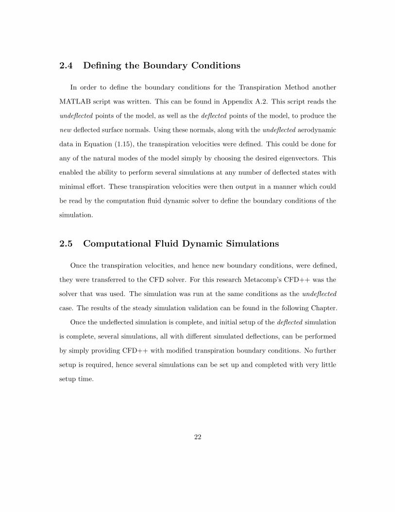
2.4 Defining the Boundary Conditions

In order to define the boundary conditions for the Transpiration Method another

MATLAB script was written. This can be found in Appendix A.2. This script reads the

undeflected points of the model, as well as the deflected points of the model, to produce the

new deflected surface normals. Using these normals, along with the undeflected aerodynamic

data in Equation (1.15), the transpiration velocities were defined. This could be done for

any of the natural modes of the model simply by choosing the desired eigenvectors. This

enabled the ability to perform several simulations at any number of deflected states with

minimal effort. These transpiration velocities were then output in a manner which could

be read by the computation fluid dynamic solver to define the boundary conditions of the

simulation.

2.5 Computational Fluid Dynamic Simulations

Once the transpiration velocities, and hence new boundary conditions, were defined,

they were transferred to the CFD solver. For this research Metacomp’s CFD++ was the

solver that was used. The simulation was run at the same conditions as the undeflected

case. The results of the steady simulation validation can be found in the following Chapter.

Once the undeflected simulation is complete, and initial setup of the deflected simulation

is complete, several simulations, all with different simulated deflections, can be performed

by simply providing CFD++ with modified transpiration boundary conditions. No further

setup is required, hence several simulations can be set up and completed with very little

setup time.

22

2.6 Unsteady Considerations

In order to perform an unsteady simulation, one that would be needed for such calcu-

lations as a flutter analysis, the boundary conditions needed to be defined at every time

step. This was done in a similar manner to the steady boundary conditions, where the

eigenvectors were used to deflect the model. To account for the model deflecting with time,

two methods were explored. The first method involved the magnitude of the transpiration

velocities which were applied to the surface of the model being scaled from zero magnitude

to maximum value at a specific frequency. This frequency corresponds to the natural

frequency of the natural mode of which the model was deflected. Hence, for Mode 1, or

First Bending, the model was deflected in this mode and the velocities varied at the first

natural frequency of the model.

The second method involved scaling the eigenvectors from zero to maximum magnitude

at the natural frequency of the natural mode of which the model was deflected. Then, using

the scaled eigenvectors at each time step, the transpiration velocities were calculated and

were applied as the boundary conditions for the corresponding time step.

This second method was determined to be a more accurate representation of the actual

deflection of the model. This is due to the fact that for the first method, it is assumed that

the transpiration velocities vary linearly with the deflection of the model. This is not the

case, and as such, calculating the transpiration velocities based on modified eigenvectors

instead of scaled maximum transpiration velocities, was chosen as the method to perform

the unsteady simulations.

23

2.7 Processing Simulation Results

User defined probes at locations along the surface of the wing were created. Within

CFD++ it is possible to define a probe location which records all the primitive variables in

the simulation at each time step and writes them to a single file. This file was read by a

MATLAB script and the data was processed using the Fast Fourier Transform, as described

in section 1.3. This script can be found in Appendix A.3.

Once this was complete, the results were used to replace the aerodynamic data obtained

by the DLM used in the structural solver to perform aeroelastic flutter analysis.

2.8 Implementation of High-Fidelity CFD Data into NAS-

TRAN

As mentioned in the previous section, once the simulation results were processed they

were then used to replace the aerodynamic data produced by the DLM. Replacing the DLM

data was done by manipulating the aerodynamic matrices NASTRAN uses to calculate its

flutter results. This method is explained in detail in Chapter 4.

24

Chapter 3

Validation of the Transpiration

Method

The validation of the Transpiration Method was done by means of two test cases.

The two cases were run at steady condition in order to first validate the ability of the

Transpiration Method in simulating deflections. The first was the BACT Wing with a

deflected trailing edge flap, and the second was a deflected AGARD 445.6 Wing. The two

cases are described below.

3.1 BACT Wing

The first validation test case was the Benchmark Active Controls Technology (BACT)

Wing, developed by The Structural Division of NASA Langley Research Centre’s Benchmark

Models Program. The dimensions of the BACT wing, along with the placement of the

control surfaces can be seen in Figure 3.1 and have been taken from Reference [5].

There are three control surfaces on the wing, a trailing edge flap and an upper and

lower surface spoiler. The control surfaces are centred along the 60% span, and are 30%

25

Figure 3.1: BACT Wing Model Dimensions [5]

the wing span. The trailing edge flap has a width of 25% the wing chord. The airfoil of the

BACT wing is the NACA 0012 symmetric airfoil.

In order to compare the transpiration method, an actually deflected trailing edge flap was

modelled. The two meshes are compared in Figures 3.2a and 3.2b. Both meshes contained

on the order of 1, 600, 000 tetrahedral cells, with concentration of the mesh at the trailing

edge flap. The increased number of cells is to improve the precision of the simulations and

to capture the flow conditions imposed by the trailing edge flap. This number is much

larger than other studies done using this method, as in reference [5], however with the

computational resources available the time required to run the simulations was not an issue.

It can be seen in Figures 3.2a and 3.2b that the deflection of the flap is significant,

at 10◦. This is to demonstrate the ability of the transpiration method to simulate large

deflections.

The simulation was executed at Mach 0.77 with the wing at an angle of attack of 0◦

and the trailing edge flap at 10◦ (downward) deflection, to match with the simulations

26

(a) Actual (b) Simulated

Figure 3.2: Deflected Trailing Edge Flap

performed in reference [5]. The results of the two simulations can be seen in Figures 3.4a

and 3.4b.

In order to ensure the convergence of the simulations, the residuals were monitored

throughout the simulations. The simulation was considered to have converged to an

acceptable level once the residuals had decreased by five orders of magnitude. The solution

residuals for the momentum are shown in Figure 3.3, for both the actually deflected flap

simulation and the transpiration method simulation, to illustrate this point. As a note,

the residuals shown are relative values, showing the five order of magnitude drop, not the

absolute values of the residuals.

Qualitatively the two pressure contours show very good agreement. This is further

illustrated by means of a comparison of the pressure distribution at a cut located at the

60% span of the wing. This is shown in Figure 3.5 below.

Figure 3.5 shows excellent agreement between the actual and simulated flap deflection,

with the only discrepancy being noted at the interface of the control surface and the wing.

This discrepancy was also noted in reference [5] and was thought to be caused by the sudden

change in geometry at the flap interface. Reference [5] stated that the fact that a Euler

solver is used for the simulation it would not be expected that any separation and boundary

27

0 50 100 150 200 25010

0

101

102

103

104

105

106

Iteration

Resid

ual

Transpiration

0 200 400 60010

−1

100

101

102

103

104

105

106

Iteration

Resid

ual

Actual Deflection

x−momentum

y−momentum

z−momentum

x−momentum

y−momentum

z−momentum

Figure 3.3: Convergence of Solution Residuals - BACT Wing

layer-shock interactions caused by the large surface deflection, would be detected. That is

to say that the transpiration method is only as accurate as the limitations of the inviscid

assumptions applied to the method.

One other explanation for the discrepancy at the control surface interface, is that the

transpiration method, as applied here, is applied to a set of panels on the control surface,

whereas in other research [5], [3], [4] it was applied to every node. This was not possible

with the tools presently in use, and was not considered to be necessary as the point of the

BACT test case was to determine if the transpiration method showed the potential to be

28

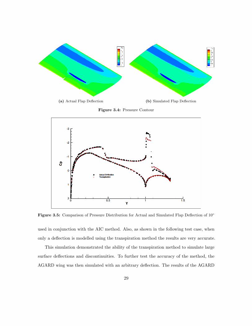
(a) Actual Flap Deflection (b) Simulated Flap Deflection

Figure 3.4: Pressure Contour

Figure 3.5: Comparison of Pressure Distribution for Actual and Simulated Flap Deflection of 10◦

used in conjunction with the AIC method. Also, as shown in the following test case, when

only a deflection is modelled using the transpiration method the results are very accurate.

This simulation demonstrated the ability of the transpiration method to simulate large

surface deflections and discontinuities. To further test the accuracy of the method, the

AGARD wing was then simulated with an arbitrary deflection. The results of the AGARD

29

wing simulations are shown in the following section.

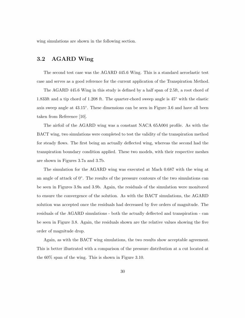
3.2 AGARD Wing

The second test case was the AGARD 445.6 Wing. This is a standard aeroelastic test

case and serves as a good reference for the current application of the Transpiration Method.

The AGARD 445.6 Wing in this study is defined by a half span of 2.5ft, a root chord of

1.833ft and a tip chord of 1.208 ft. The quarter-chord sweep angle is 45◦ with the elastic

axis sweep angle at 43.15◦. These dimensions can be seen in Figure 3.6 and have all been

taken from Reference [10].

The airfoil of the AGARD wing was a constant NACA 65A004 profile. As with the

BACT wing, two simulations were completed to test the validity of the transpiration method

for steady flows. The first being an actually deflected wing, whereas the second had the

transpiration boundary condition applied. These two models, with their respective meshes

are shown in Figures 3.7a and 3.7b.

The simulation for the AGARD wing was executed at Mach 0.687 with the wing at

an angle of attack of 0◦. The results of the pressure contours of the two simulations can

be seen in Figures 3.9a and 3.9b. Again, the residuals of the simulation were monitored

to ensure the convergence of the solution. As with the BACT simulations, the AGARD

solution was accepted once the residuals had decreased by five orders of magnitude. The

residuals of the AGARD simulations - both the actually deflected and transpiration - can

be seen in Figure 3.8. Again, the residuals shown are the relative values showing the five

order of magnitude drop.

Again, as with the BACT wing simulations, the two results show acceptable agreement.

This is better illustrated with a comparison of the pressure distribution at a cut located at

the 60% span of the wing. This is shown in Figure 3.10.

30

Elastic axis

Quarter-chord line

2.5

1.208

45°

43.15°

1.833

Figure 3.6: AGARD Wing Model Dimensions

Once again, with the simulation of an arbitrarily deflected AGARD wing, the transpi-

ration method has shown to provide well matching results when compared to an actually

deflected model. The final validation case was to apply this method to the Global Express

wing. The results from this test were not as good as the previous cases, however, the trends

suggested that the method would perform well if more time was spent refining the model

31

(a) Actual (b) Simulated

Figure 3.7: AGARD Wing

0 20 40 60 80 10010

0

101

102

103

104

105

Iteration

Resid

ual

Transpiration

0 20 40 60 80 10010

0

101

102

103

104

105

106

Iteration

Resid

ual

Actual Deflection

x−momentum

y−momentum

z−momentum

x−momentum

y−momentum

z−momentum

Figure 3.8: Convergence of Solution Residuals - AGRAD Wing

32

(a) Actual (b) Simulated

Figure 3.9: Pressure Contour for Deflection of AGARD Wing

+

+

+++

++

++

++

+++++

+

++++

+

+

+

+++

+

++

+

+++

++

+++

++++++

+

+++++++ ++++ +++ + +++

++++++++ ++ + ++ +++ ++ ++++ ++++++ + +++ ++ + ++

++ ++++ +++++

+++ + ++++++

+++ +++++

+++++++++

+ + ++ + ++ ++ +++

++++

+++

+ + ++ ++ + + + + ++++ + ++ +++++ +

+++++ + +++ +++++ +++++++++++++

+

++

+

+

++

++++

+

++

+++

++

+++

+++

++++

+++++++++++

+++++++

++++++++

+++++

+ ++++++ ++++++

+ +++ +++ + ++++++ ++ ++ + + ++++ ++ +++ +++++ +

+++ ++++ ++++ +++ ++ +++ + + +++ ++ + + + ++ ++ + + ++ ++++ ++

++ + +++++++ + ++ ++ ++++ + +++ ++ ++ +++ ++++++++++

++++++++

X

Cp

1.4 1.6 1.8 2 2.2 2.4 2.6 2.8 3 3.2

­2

­1.5

­1

­0.5

0

0.5

1

1.5

Actually DeflectedTranspiration+

Figure 3.10: Comparison of Pressure Distribution for Actual and Simulated Deflection of AGARDWing

and technique for this case. This was forgone in respect to time constraints of this research.

The results obtained from the steady validation cases provided sufficient information

that this method is suitable for the use of deforming the aerodynamic model at each time

step in an unsteady simulation. The results of unsteady simulations of an AGARD wing

experiencing flutter are presented in section 5.2

33

Chapter 4

Modal Based AIC Method in

NASTRAN

In order to incorporate the modal-based AIC method into an aeroelastic solver it must

be redefined from its purely aerodynamic development. This aerodynamic development was

described in section 1.5. As mentioned in previous sections, the aeroelastic solver used in

this thesis for the structural calculations is NASTRAN. Using the definition of aerodynamic

matrices, shown in section 1.2.3, the modal-based AIC method is defined for use with

NASTRAN.

4.1 Background

This method begins with the definition of the generalized aerodynamic matrix, [Qhh],

which describes the aerodynamics of the model. This is shown below as Equation (4.1),

now renamed from the original Equation (1.6) to match the naming convention used within

NASTRAN.

[Qhh] = [φgh]T [Gkg]T [WTFACT ] [Qkk] [Gkg] [φgh] (4.1)

34

This generalized aerodynamic matrix is an essential part of the flutter analysis and

calculations performed by NASTRAN. This generalized aerodynamic matrix is the matrix to

be altered by the modal-based AIC method to in turn alter the flutter results for a different

modal configuration. Within the generalized aerodynamic matrix is the aerodynamic

influence matrix, [Qkk]. This matrix was previously defined as Equation (1.5). This matrix

is formed in NASTRAN and is explained in section 1.2.3.

This AIC matrix can then be multiplied by the interpolated mode shapes, represented

by the combination of the Interpolation Matrix [Gkg], and the Normal mode vectors [φgh].

This then produces a new matrix, [Qkh] and is shown in Equation (4.2) below:

[Qkh] = [Skj ] [Ajj ]−1 [Djk

1 + ikDjk2]

[Gkg] [φgh] (4.2)

This [Qkh] matrix contains the information of the variation of lifts, ∆Cl and moments,

∆Cm on each aerodynamic panel for each of the chosen h modes. It is then possible to collect

this same data from high-fidelity CFD solvers and replace this data which is calculated

using the DLM with the goal of providing more accurate aerodynamic data and hence

producing more accurate aeroelastic results and analysis.

It is also possible to use the [Qjh] matrix, which contains information on the variation

of pressure ∆Cp, on each of the aerodynamic panels, however, it was determined in previous

research [15] that the use of the [Qkh] matrix is the optimal method to transfer the high-

fidelity CFD data to NASTRAN, and as so the [Qkh] matrix is also used in this research.

The [Qjh] matrix is defined below for reference in Equation (4.3).

[Qjh] = [Ajj ]−1 [Djk

1 + ikDjk2]

[Gkg] [φgh] (4.3)

In a similar manner to that described in section 1.5, the [Qkh] can be used in place of the

35

∆Cp vector, along with the Normal mode vectors [φgh] to produce the following equation.

[Qkh] = [Qkg] [φgh] (4.4)

Within this equation the modal-based AIC matrix is defined. To remain consistent with

the NASTRAN naming convention, it is called the [Qkg] matrix. This [Qkg] matrix is the

aerodynamic base for all configurations of the model. This aerodynamic base can then be

used in a similar manner to that developed by Chen et al. [16]. The [Qkg] matrix, which is

the base for all model configurations, and hence remains constant for all configurations,

can then be used in combination with other configuration’s mode shapes to produce the

variation of lifts and moments on each of the aerodynamic panels for the new configuration.

In order to calculate this aerodynamic base, the [Qkh] matrix is used along with the

Normal mode vectors [φgh]. This is where the aerodynamic base, [Qkg] matrix will be

modified with the high-fidelity CFD data through the [Qkh] matrix. This is done by means

of the least-square procedure outlined in section 1.5. The equation for the aerodynamic

base of configuration 1 is then

[Qkg]1 = [Qkh]1

[(φgh

Tφgh)−1

φghT]1

(4.5)

The accuracy of the calculated aerodynamic base, [Qkg] is obviously dependant on the

accuracy of the lifts and moments given in the [Qkh] matrix and the number of mode shapes

used in the Normal mode vector [φgh].

Now, using this newly calculated aerodynamic base, which incorporates the high-fidelity

CFD data, the lifts and moments can be calculated for a second configuration of the model,

36

given the new configuration’s Normal mode vector [φgh]2, through:

[Qkh]2 = [Qkg]1[φgh]2 (4.6)

Finally, this [Qkh]2 matrix can be used in Equation (4.1), rewritten as Equation (4.7)

below, to calculate the new flutter results of configuration 2, or any desired configuration.

[Qhh]2 = [φgh]T [Gkg]T [WTFACT ] [Qkh]2 (4.7)

The weighting factor, [WTFACT ], as previously explained, is needed if only steady

aerodynamic analysis is completed using high-fidelity CFD. As both steady and unsteady

aerodynamic analyses were performed in this research this weighting factor is not needed.

4.2 Lifts and Moments

In order to validate the accuracy of the modal-based AIC method described in the

previous section, a comparison of the lifts and moments, or rather the variation of lifts and

moments, ∆Cl and ∆Cm respectively, was undertaken between the results generated by the

method and the results generated by the Doublet Lattice Method within NASTRAN. This

was first done for the steady simulations. This was also completed to validate the work

done previously [15].

The validation the modal-based AIC method for steady simulations was done by choosing

two configurations of the AGARD wing model. These configurations differed by the stiffness

of the model, and hence the mode shapes and natural frequencies of the two configurations

were different. Then, using NASTRAN the aerodynamic data was produced by means of

the DLM for the two configurations. This aerodynamic data was extracted for the first

four natural modes of the wing. The first four modes shapes were chosen as the base for

37

the modal-based AIC method as they were found to have the greatest influence on the

wing flutter mechanism, this was also noted in previous research [15]. With the DLM

aerodynamic data extracted from the four base modes, the [Qkh] matrix could then be

modified as stated in Equation (4.6) to produce the second configuration’s change in lift

and moments.

The results of the steady simulations as applied to the modal-based AIC method can be

seen in the Figures 4.1 through 4.8 as the real lifts and moments for the first four natural

modes are plotted. The figures show three cuts along the span of the AGARD wing, one

at the root, one at the centre and finally one at the tip. The wing was divided into 240

panels numbered 1 to 240 starting at the leading edge root to the trailing edge tip of the

wing. In all of the following figures the two actually deflected configurations of the AGARD

wing are denoted as Configuration 1 and Configuration 2, respectively, whereas the AIC

approximation of the second configuration of the AGARD wing is denoted as AIC 2. This

is to not over crowd the legends in the figures.

It can be seen in Figures 4.1 and 4.2 that for the first natural mode the modal-based

AIC approximation of the second configuration is very close. There is little difference

between the high-fidelity CFD results for the second natural mode and the modal-based

AIC approximation.

For the second natural mode, shown in Figures 4.3 and 4.4, the results are also close.

With the agreement between the AIC approximation and the actual high-fidelity CFD being

acceptable. This trend continues in with the third mode in Figures 4.5 and 4.6.

The agreement between the two methods is still very good for the third natural mode.

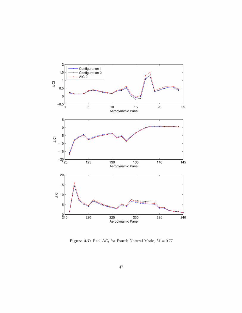
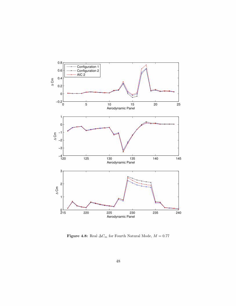
The results of the fourth natural mode are shown in Figures 4.7 and 4.8. Here it can be

seen that the agreement between the high-fidelity CFD results and the AIC approximation

is not as good as the previous modes. It can be seen in Figure 4.7 that the approximation

38

of lifts near the root of the wing shows a large discrepancy, but the approximation improves

as one moves along the wing. The change in moments, in Figure 4.8 show the same trend

as the lifts, giving a poor approximation near the root. This discrepancy is due to the

fact that only four modes were used to produce the modal-based AIC matrix, [Qkg]. As

described in Equation (4.5) the accuracy of the approximation is directly affected by the

number of modes used. This was discussed in depths in Reference [15].

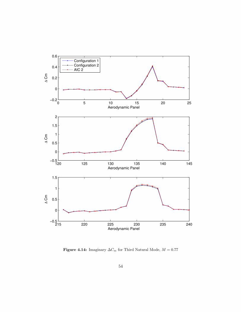
4.3 Unsteady Lifts and Moments

The next part of the validation of the modal-based AIC method was to evaluate the

unsteady, or imaginary changes in lifts and moments. This was done by comparing the

imaginary parts of the change in lift and moment coefficient similar to the method used

for the steady, or real, lift and moment comparison. The same two configurations of the

AGARD wing were chosen and the modal-based AIC method was used to modify the [Qkh]

matrix. The results and comparison of the modal-based AIC can be seen in the Figures 4.9

through 4.16.

It can be seen in the figures above that the comparison of the unsteady modal-based

AIC method to the DLM results show satisfactory agreement. This is similar to the steady

comparison. The only major deviation in the comparison is once again at the root of the

wing for the fourth mode. This is again explained by the fact that only four modes were

used when constructing the aerodynamic base for the method as explained in detail in

Reference [15].

The results of both the steady and unsteady AIC approximations show that the modal-

based AIC method is suitable for approximating different aircraft configurations. The goal

of this research was not to prove the validity if this method, as that was studied extensively

in Reference [15], but to study the effect of adding unsteady aerodynamic data to the

39

modal-based AIC method. This is true for the addition of high-fidelity CFD data to the

method as well.

40

0 5 10 15 20 25−1

−0.5

0

0.5

Aerodynamic Panel

∆ C

l

Configuration 1

Configuration 2

AIC 2

120 125 130 135 140 145−4

−3

−2

−1

0

Aerodynamic Panel

∆ C

l

215 220 225 230 235 240−6

−4

−2

0

Aerodynamic Panel

∆ C

l

Figure 4.1: Real ∆Cl for First Natural Mode, M = 0.77

41

0 5 10 15 20 25−0.6

−0.4

−0.2

0

0.2

Aerodynamic Panel

∆ C

m

Configuration 1

Configuration 2

AIC 2

120 125 130 135 140 145−1.5

−1

−0.5

0

Aerodynamic Panel

∆ C

m

215 220 225 230 235 240−0.5

−0.4

−0.3

−0.2

−0.1

0

Aerodynamic Panel

∆ C

m

Figure 4.2: Real ∆Cm for First Natural Mode, M = 0.77

42

0 5 10 15 20 25−1.5

−1

−0.5

0

Aerodynamic Panel

∆ C

l

120 125 130 135 140 1450

2

4

6

8

Aerodynamic Panel

∆ C

l

215 220 225 230 235 2400

5

10

15

20

Aerodynamic Panel

∆ C

l

Configuration 1

Configuration 2

AIC 2

Figure 4.3: Real ∆Cl for Second Natural Mode, M = 0.77

43

0 5 10 15 20 25−0.8

−0.6

−0.4

−0.2

0

Aerodynamic Panel

∆ C

m

120 125 130 135 140 1450

1

2

3

Aerodynamic Panel

∆ C

m

215 220 225 230 235 2400

0.5

1

1.5

2

Aerodynamic Panel

∆ C

m

Configuration 1

Configuration 2

AIC 2

Figure 4.4: Real ∆Cm for Second Natural Mode, M = 0.77

44

0 5 10 15 20 250

5

10

15

20

Aerodynamic Panel

∆ C

l

120 125 130 135 140 1450

10

20

30

40

50

Aerodynamic Panel

∆ C

l

215 220 225 230 235 240−20

0

20

40

60

80

Aerodynamic Panel

∆ C

l

Configuration 1

Configuration 2

AIC 2

Figure 4.5: Real ∆Cl for Third Natural Mode, M = 0.77

45

0 5 10 15 20 250

2

4

6

8

10

Aerodynamic Panel

∆ C

m

120 125 130 135 140 1450

5

10

15

20

Aerodynamic Panel

∆ C

m

215 220 225 230 235 240−2

0

2

4

6

8

Aerodynamic Panel

∆ C

m

Configuration 1

Configuration 2

AIC 2

Figure 4.6: Real ∆Cm for Third Natural Mode, M = 0.77

46

0 5 10 15 20 25−0.5

0

0.5

1

1.5

2

Aerodynamic Panel

∆ C

l

120 125 130 135 140 145−20

−15

−10

−5

0

5

Aerodynamic Panel

∆ C

l

215 220 225 230 235 2400

5

10

15

20

Aerodynamic Panel

∆ C

l

Configuration 1

Configuration 2

AIC 2

Figure 4.7: Real ∆Cl for Fourth Natural Mode, M = 0.77

47

0 5 10 15 20 25−0.2

0

0.2

0.4

0.6

0.8

Aerodynamic Panel

∆ C

m

120 125 130 135 140 145−4

−3

−2

−1

0

1

Aerodynamic Panel

∆ C

m

215 220 225 230 235 2400

1

2

3

Aerodynamic Panel

∆ C

m

Configuration 1

Configuration 2

AIC 2

Figure 4.8: Real ∆Cm for Fourth Natural Mode, M = 0.77

48

0 5 10 15 20 25−0.2

−0.15

−0.1

−0.05

0

0.05

Aerodynamic Panel

∆ C

l

Configuration 1

Configuration 2

AIC 2

120 125 130 135 140 145−1

−0.8

−0.6

−0.4

−0.2

0

Aerodynamic Panel

∆ C

l

215 220 225 230 235 240−1.5

−1

−0.5

0

Aerodynamic Panel

∆ C

l

Figure 4.9: Imaginary ∆Cl for First Natural Mode, M = 0.77

49

0 5 10 15 20 25−0.1

−0.08

−0.06

−0.04

−0.02

0

Aerodynamic Panel

∆ C

m

Configuration 1

Configuration 2

AIC 2

120 125 130 135 140 145−0.4

−0.3

−0.2

−0.1

0

Aerodynamic Panel

∆ C

m

215 220 225 230 235 240−0.25

−0.2

−0.15

−0.1

−0.05

0

Aerodynamic Panel

∆ C

m

Figure 4.10: Imaginary ∆Cm for First Natural Mode, M = 0.77

50

0 5 10 15 20 25−0.5

−0.4

−0.3

−0.2

−0.1

0

Aerodynamic Panel

∆ C

l

120 125 130 135 140 145−2

−1

0

1

Aerodynamic Panel

∆ C

l

215 220 225 230 235 240−0.5

0

0.5

1

1.5

Aerodynamic Panel

∆ C

l

Configuration 1

Configuration 2

AIC 2

Figure 4.11: Imaginary ∆Cl for Second Natural Mode, M = 0.77

51

0 5 10 15 20 25−0.25

−0.2

−0.15

−0.1

−0.05

0

Aerodynamic Panel

∆ C

m

120 125 130 135 140 145−0.4

−0.2

0

0.2

0.4

Aerodynamic Panel

∆ C

m

215 220 225 230 235 240−0.1

0

0.1

0.2

0.3

0.4

Aerodynamic Panel

∆ C

m

Configuration 1

Configuration 2

AIC 2

Figure 4.12: Imaginary ∆Cm for Second Natural Mode, M = 0.77

52

0 5 10 15 20 25−0.5

0

0.5

1

Aerodynamic Panel

∆ C

l

120 125 130 135 140 145−4

−2

0

2

4

6

Aerodynamic Panel

∆ C

l

215 220 225 230 235 240−4

−2

0

2

4

Aerodynamic Panel

∆ C

l

Configuration 1

Configuration 2

AIC 2

Figure 4.13: Imaginary ∆Cl for Third Natural Mode, M = 0.77

53

0 5 10 15 20 25−0.2

0

0.2

0.4

0.6

Aerodynamic Panel

∆ C

m

120 125 130 135 140 145−0.5

0

0.5

1

1.5

2

Aerodynamic Panel

∆ C

m

215 220 225 230 235 240−0.5

0

0.5

1

1.5

Aerodynamic Panel

∆ C

m

Configuration 1

Configuration 2

AIC 2

Figure 4.14: Imaginary ∆Cm for Third Natural Mode, M = 0.77

54

0 5 10 15 20 250

0.1

0.2

0.3

0.4

0.5

Aerodynamic Panel

∆ C

l

120 125 130 135 140 145−2

−1

0

1

Aerodynamic Panel

∆ C

l

215 220 225 230 235 240−0.5

0

0.5

1

1.5

2

Aerodynamic Panel

∆ C

l

Configuration 1

Configuration 2

AIC 2

Figure 4.15: Imaginary ∆Cl for Fourth Natural Mode, M = 0.77

55

0 5 10 15 20 250

0.05

0.1

0.15

0.2

0.25

Aerodynamic Panel

∆ C

m

120 125 130 135 140 145−0.8

−0.6

−0.4

−0.2

0

0.2

Aerodynamic Panel

∆ C

m

215 220 225 230 235 240−0.2

0

0.2

0.4

0.6

Aerodynamic Panel

∆ C

m

Configuration 1

Configuration 2

AIC 2

Figure 4.16: Imaginary ∆Cm for Fourth Natural Mode, M = 0.77

56

Chapter 5

Validation of High-Fidelity CFD

Results

The aerodynamic information used in the flutter analysis is produced using the Doublet

Lattice Method, which is incorporated into the structural solver. As stated, for this thesis

the structural solver used was NASTRAN. This DLM aerodynamic information is to be

replaced by that of high fidelity CFD data. This is done through the variation of lifts

and moments produced by the deflection of the structure by its natural modes. This was

explained in the previous Chapter. In order to obtain these variations, the model must be

deformed by the natural modes and the pressure distributions must be compared to that

of the undeflected structure to obtain the ∆Cl and ∆Cm which are included in the [Qkh]

matrix.

5.1 Defining the Deflected Model

In order to obtain the deformed shape of the structure a modal analysis of the structure

must first be performed. This was done using NASTRAN. First the structure was modelled

57

as a two dimensional structure with the same divisions as the high fidelity CFD model.

This 2D model was then analyzed and the natural modes were extracted. This included the

eigenvectors for the deflections of each mode. Once these eigenvectors were calculated they

were then used in a MATLAB script to deflect the CFD model and create the transpiration

method boundary conditions. This was all done in a similar manner to that explained in

Chapter 2.

5.2 Results and Comparison to DLM

The high-fidelity CFD results produced by the transpiration method were compared

to those of the DLM to ensure that the method was at least as good as present method

for aerodynamic analysis. This was done for both steady and unsteady simulations. For

comparison of the steady simulations the change in lift and moment coefficient between

the undeflected and deflected structure for each of the different modes along the span

of the wing was compared. Also, the variation of lift and moment at each aerodynamic

panel was compared. For the unsteady simulations, the comparison was made for the real

and imaginary change in lift and moment. These results for both steady and unsteady

simulations can be seen in the following sections.

5.2.1 Steady Simulations

The steady simulations were validated against the results produced by means of the

DLM by plotting the variation of coefficient of lift, ∆Cl, and coefficient of moment, ∆Cm,

along the span of the wing, as well as for each aerodynamic panel, for the different modes

studied. As with the validation of the transpiration method performed in earlier sections,

the simulations were considered to have converged when the residuals had decreased by five

orders of magnitude. These results are shown in the Figures 5.1 through 5.8.

58

1 2 3 4 5 6 7 8 9 10−40

−35

−30

−25

−20

−15

−10

−5

∆ C

l

Wing Span

∆ Cl per strip for first natural mode at M=0.77

1 2 3 4 5 6 7 8 9 102

3

4

5

6

7

8

9

∆ C

m

Wing Span

∆ Cm per strip for first natural mode at M=0.77

High−Fidelity CFD

DLM

High−Fidelity CFD

DLM

Figure 5.1: Spanwise Comparison of high-fidelity CFD and DLM results for First Natural Mode,M = 0.77

0 50 100 150 200 250−6

−5

−4

−3

−2

−1

0

1

∆ C

l

Wing Span

∆ Cl per panel for first natural mode at M=0.77

0 50 100 150 200 250−0.5

0

0.5

1

1.5

∆ C

m

Wing Span

∆ Cm per panel for first natural mode at M=0.77

High−Fidelity CFD

DLM

High−Fidelity CFD

DLM

Figure 5.2: Panel Comparison of high-fidelity CFD and DLM results for First Natural Mode,M = 0.77

59

1 2 3 4 5 6 7 8 9 10−50

0

50

100

150

∆ C

l

Wing Span

∆ Cl per strip for second natural mode at M=0.77

1 2 3 4 5 6 7 8 9 10−30

−20

−10

0

10

20

∆ C

m

Wing Span

∆ Cm per strip for second natural mode at M=0.77

High−Fidelity CFD

DLM

High−Fidelity CFD

DLM

Figure 5.3: Spanwise Comparison of high-fidelity CFD and DLM results for Second Natural Mode,M = 0.77

0 50 100 150 200 250−5

0

5

10

15

20

∆ C

l

Wing Span

∆ Cl per panel for second natural mode at M=0.77

0 50 100 150 200 250−4

−3

−2

−1

0

1

2

3

∆ C

m

Wing Span

∆ Cm per panel for second natural mode at M=0.77

High−Fidelity CFD

DLM

High−Fidelity CFD

DLM

Figure 5.4: Panel Comparison of high-fidelity CFD and DLM results for Second Natural Mode,M = 0.77

60

1 2 3 4 5 6 7 8 9 10100

200

300

400

500

∆ C

l

Wing Span

∆ Cl per strip for third natural mode at M=0.77

1 2 3 4 5 6 7 8 9 10−120

−100

−80

−60

−40

∆ C

m

Wing Span

∆ Cm per strip for third natural mode at M=0.77

High−Fidelity CFD

DLM

High−Fidelity CFD

DLM

Figure 5.5: Spanwise Comparison of high-fidelity CFD and DLM results for Third Natural Mode,M = 0.77

0 50 100 150 200 250−10

0

10

20

30

40

50

60

∆ C

l

Wing Span

∆ Cl per panel for third natural mode at M=0.77

0 50 100 150 200 250−25

−20

−15

−10

−5

0

5

∆ C

m

Wing Span

∆ Cm per panel for third natural mode at M=0.77

High−Fidelity CFD

DLM

High−Fidelity CFD

DLM

Figure 5.6: Panel Comparison of high-fidelity CFD and DLM results for Third Natural Mode,M = 0.77

61

1 2 3 4 5 6 7 8 9 10−150

−100

−50

0

50

100

150

∆ C

l

Wing Span

∆ Cl per strip for fourth natural mode at M=0.77

1 2 3 4 5 6 7 8 9 10−30

−20

−10

0

10

20

30

∆ C

m

Wing Span

∆ Cm per strip for fourth natural mode at M=0.77

High−Fidelity CFD

DLM

High−Fidelity CFD

DLM

Figure 5.7: Spanwise Comparison of high-fidelity CFD and DLM results for Fourth Natural Mode,M = 0.77

0 50 100 150 200 250−20

−15

−10

−5

0

5

10

15

∆ C

l

Wing Span

∆ Cl per panel for fourth natural mode at M=0.77

0 50 100 150 200 250−4

−2

0

2

4

6

∆ C

m

Wing Span

∆ Cm per panel for fourth natural mode at M=0.77

High−Fidelity CFD

DLM

High−Fidelity CFD

DLM

Figure 5.8: Panel Comparison of high-fidelity CFD and DLM results for Fourth Natural Mode,M = 0.77

62

The results of the transpiration method compare well with the DLM results. There are

only minor differences in the change in lift and moment produced by the modal deflections.

There are some discrepancies with the lift and moment distribution along the span of the

wing. These discrepancies may be accounted for by the manner in which the two values

were computed, the DLM and high-fidelity CFD. The DLM may have not captured some

3D effects that the high-fidelity CFD was able to model. Also, at Mach of 0.77 it would not

be expected that shocks would form, however if this were the case then differences between

the two methods would be expected. This is something that will need to be examined more

thoroughly with more simulations. From the agreement between the two methods for the

change in lift and moment at each panel, in combination with the validation performed in

Chapter 3, it can be said that the transpiration method will provide suitable aerodynamic

results for use with the modal-based AIC method. This statement is further reinforced by

examining the unsteady simulation results presented in the next section.

5.2.2 Unsteady Simulations

The unsteady simulations were validated by comparison of the real and imaginary

components of lift and moment to those produced by the DLM. The real and imaginary

components of lift and moment were extracted in the manner explained in Section 1.3

for the high-fidelity CFD simulations. Once the high-fidelity CFD values were obtained,

the values from the DLM needed to be extracted. The DLM values were extracted from

NASTRAN by means of a DMAP alter, a subroutine that is added during flutter analysis

to output the [Qkh] matrix used in the flutter calculations. This is a matrix which is not

usually output by NASTRAN and as such is difficult to obtain. The convergence of the

unsteady simulations were monitored at each global time step. For each global time step

the simulation was run for 20 internal time steps. This allowed for the residuals to decrease

63

by at least one order of magnitude, however, it was usually two orders magnitude or more.

The results of the comparison between the high-fidelity CFD and DLM results for unsteady

components of lift and moments for the first four natural modes can be seen in the figures

below.

0 50 100 150 200 250−6

−5

−4

−3

−2

−1

0

1

∆ C

l

Wing Span

∆ Cl per panel for first natural mode at M=0.77

0 50 100 150 200 250−0.5

0

0.5

1

1.5

∆ C

m

Wing Span

∆ Cm per panel for first natural mode at M=0.77

High−Fidelity CFD

DLM

High−Fidelity CFD

DLM

Figure 5.9: Comparison of Real and Imaginary ∆Cl for First Natural Mode, M = 0.77

For the real and imaginary components of lift and moment there is a good agreement,

for the most part, between the transpiration method and the DLM. With large differences

being found only in Figures 5.13 and 5.14, the imaginary component of lift and moment for

mode 3 respectively. It appears as if there is an inflection in the lifts and moments that

does not appear in the DLM data. This inflection may be due to the way in which the mode

shapes were applied to the boundary conditions; further unsteady analysis is required.

As previously mentioned, the goal of this research was to incorporate unsteady aero-

dynamic data to the modal-based AIC method, not to prove the Transpiration method.

The Transpiration method was used for the unsteady aerodynamic calculations because

64

0 50 100 150 200 250−1.5

−1

−0.5

0

0.5

∆ C

m

Aerodynamic Panel

Real ∆ Cm per panel for first natural mode at M=0.77

0 50 100 150 200 250−0.5

−0.4

−0.3

−0.2

−0.1

0

0.1

∆ C

m

Aerodynamic Panel

Imaginary ∆ Cm per panel for first natural mode at M=0.77

High−Fidelity CFD

DLM

Figure 5.10: Comparison of Real and Imaginary ∆Cm for First Natural Mode, M = 0.77

0 50 100 150 200 250−10

−5

0

5

10

15

20

∆ C

l

Aerodynamic Panel

Real ∆ Cl per panel for second natural mode at M=0.77

0 50 100 150 200 250−2

−1

0

1

2

3

∆ C

l

Aerodynamic Panel

Imaginary ∆ Cl per panel for second natural mode at M=0.77

High−Fidelity CFD

DLM

Figure 5.11: Comparison of Real and Imaginary ∆Cl for Second Natural Mode, M = 0.77

65

0 50 100 150 200 250−1

0

1

2

3

4

5

∆ C

m

Aerodynamic Panel

Real ∆ Cm per panel for second natural mode at M=0.77

0 50 100 150 200 250−0.6

−0.4

−0.2

0

0.2

0.4

0.6

∆ C

m

Aerodynamic Panel

Imaginary ∆ Cm per panel for second natural mode at M=0.77

High−Fidelity CFD

DLM

Figure 5.12: Comparison of Real and Imaginary ∆Cm for Second Natural Mode, M = 0.77

0 50 100 150 200 250−20

0

20

40

60

80

∆ C

l

Aerodynamic Panel

Real ∆ Cl per panel for third natural mode at M=0.77

0 50 100 150 200 250−4

−2

0

2

4

6

8

∆ C

l

Aerodynamic Panel

Imaginary ∆ Cl per panel for third natural mode at M=0.77

High−Fidelity CFD

DLM

Figure 5.13: Comparison of Real and Imaginary ∆Cl for Third Natural Mode, M = 0.77

66

0 50 100 150 200 250−5

0

5

10

15

20

25

∆ C

m

Aerodynamic Panel

Real ∆ Cm per panel for third natural mode at M=0.77

0 50 100 150 200 250−2

−1

0

1

2

3

∆ C

m

Aerodynamic Panel

Imaginary ∆ Cm per panel for third natural mode at M=0.77

High−Fidelity CFD

DLM

Figure 5.14: Comparison of Real and Imaginary ∆Cm for Third Natural Mode, M = 0.77

0 50 100 150 200 250−20

−15

−10

−5

0

5

10

15

∆ C

l

Aerodynamic Panel

Real ∆ Cl per panel for fourth natural mode at M=0.77

0 50 100 150 200 250−3

−2

−1

0

1

2

3

4

∆ C

l

Aerodynamic Panel

Imaginary ∆ Cl per panel for fourth natural mode at M=0.77

High−Fidelity CFD

DLM

Figure 5.15: Comparison of Real and Imaginary ∆Cl for Fourth Natural Mode, M = 0.77

67

0 50 100 150 200 250−6

−4

−2

0

2

4

6

∆ C

m

Aerodynamic Panel

Real ∆ Cm per panel for fourth natural mode at M=0.77

0 50 100 150 200 250−1

−0.5

0

0.5

1

1.5

∆ C

m

Aerodynamic Panel

Imaginary ∆ Cm per panel for fourth natural mode at M=0.77

High−Fidelity CFD

DLM

Figure 5.16: Comparison of Real and Imaginary ∆Cm for Fourth Natural Mode, M = 0.77

of the immense time saving enjoyed by not needing to remesh the computational domain

at each time step. The results presented above show acceptable agreement with current

DLM aerodynamic calculations and hence show promise for use with the modal-based

AIC method. In future work, the unsteady aerodynamic calculations may be replaced by

more accurate simulations, incorporating Navier-Stokes solvers, as the framework of adding

unsteady data is now in place.

68

Conclusions

It was determined that a more cost and labor effective tool needed to be developed In-

House to perform aeroelastic analysis at Bombardier. For this reason the Controlled Facilities

Engineering Services and Dynamics Groups at Bombardier Aerospace have developed a

methodology to analyze flutter response of aircraft. This method was developed to be used

with aerodynamic data obtained from the Doublet Lattice Method, which is included in the

structural solver in use by Bombardier and has proven to be very useful in preliminary stages

of an aircraft design program at Bombardier. The limitations introduced by the Doublet

Lattice Method have made high-fidelity Computation Fluid Dynamic (CFD) aerodynamic

data a necessity.

Steady high-fidelity CFD data had previously been incorporated into the flutter calcula-

tions through the modal-based improved Aerodynamic Influence Coefficient (AIC) method.

The addition of steady high-fidelity CFD data proved to give improved results for flutter

calculations in the subsonic regime. For the transonic and supersonic regimes the results

were not as reliable. This is where the need for unsteady high-fidelity CFD data comes.

The incorporation of unsteady aerodynamic data to the methodology will provide more

accurate results in the transonic and supersonic regimes. In order to obtain this unsteady

high-fidelity CFD data, the Transpiration Method was investigated.

Significant work has been completed on implementing the Transpiration Method into

69

both steady and unsteady computational fluid dynamic analysis. This work includes the

simulation of static deflections with acceptable agreement to actually deflected CFD models.

This was shown through the simulation of a flap deflection of the BACT wing and an

arbitrary deflection of the AGARD wing.

The Transpiration Method was also shown to be viable in unsteady CFD simulations,

with results of modal deflections matching well with previous method results. Although

the Transpiration Method proved to show promise in unsteady CFD simulations, there are

still limitations that are imposed by the fact that the Transpiration Method must employ

an Euler solver and hence inviscid assumptions are applied to the simulations. This is due

to the fact that, as the method is implemented in this research, the surface velocities are

modified in order to simulate surface deflections and hence the no-slip condition on the

surface may not be applied. This assumption of inviscid flow may lead to the inability to

capture all shock related flow conditions. Despite this, the incorporation of an Euler solver

is still much improved to that of the two-dimensional DLM solver which is currently in use

at Bombardier.

The modal-based AIC method was applied to the aerodynamic matrices used in

NASTRAN. Using aerodynamic data from the Doublet Lattice Method, the modal-based

AIC method displayed the ability to approximate aerodynamic loads of different structural

models by use of an aerodynamic base set of modal information.

Implementation of the modal-based AIC method with high-fidelity CFD data was

accomplished. Modified aerodynamic matrices were produced for use in NASTRAN to

perform flutter analysis of several structural configurations.

Several difficulties were encountered during this research leading to final results being

unobtainable. That is, the flutter results using the modal-based AIC method were not

able to be obtained. This includes analysis with aerodynamic data from either DLM or

70

high-fidelity CFD. The main reason for this difficulty was due to the incorporation of

the unsteady aerodynamic data into the aerodynamic matrices in NASTRAN. Previous

work included only steady data, and the addition of unsteady data proved to be more

difficult than originally anticipated. Work is continuing with this, and preliminary flutter

analysis results from the modal-based AIC method with the incorporation of high-fidelity

CFD data has been completed. These preliminary results show expected trends in the

flutter mechanism behaviour, however, due to the uncertainty of the implementation of the

high-fidelity CFD data, these results will need to be further investigated. Further work is

to be done with flutter results obtained at different reduced frequencies.

Work is also being completed on obtaining and validating transonic unsteady high-fidelity

CFD data, using the Transpiration Method.

The work accomplished in this project has furthered the development of the modal-based

AIC method as applied to dynamic aeroelastic analysis using NASTRAN at Bombardier

Aerospace. The Transpiration Boundary Condition Method has been shown to be a viable

tool in performing unsteady aerodynamic analysis, and that this data may be used in the

modal-based AIC method. More work must be completed on implementing the unsteady

aerodynamic data into NASTRAN for flutter analysis, as well as further investigations of

transonic aerodynamic analysis.

71

Bibliography

[1] ZAERO Theoretical Manual.

[2] ANSYS Inc. ANSYS CFX-Solver Manager User’s Guide, 13.0 edition, November 2010.

[3] Fisher C.F. Application of the transpiration method for efficient aeroelastic analysis

using an euler solver. Master’s thesis, Oklahoma State University, Oklahoma, 1996.

[4] Fisher C.F. and Arena A.S. On the transpiration method for efficient aeroelastic

analysis using an euler solver. In AIAA 96-3436. American Institute of Aeronautics

and Astronautics, July 1996.

[5] Stephens C.H. Cfd-based aeroservoelastic predictions on a benchmark configuration

using the transpiration method. Master’s thesis, Oklahoma State University, Oklahoma,

1998.

[6] CMSoft. AERO for Powerful Multi-Physics Solutions.

[7] Arfken G. Rayleigh-Ritz Variational Technique, pages 957–961. Mathematical Methods

for Physicists. Academic Press, 3rd edition, 1985.

[8] Hassig H.J. An approximate true damping solution of the flutter equation by determi-

nant iteration. Journal of Aircraft, 8(11):885–889, November 1971.

72

[9] Anderson J.D. Fundamentals of Aerodynamics. McGraw-Hill, 4th edition, 2009.

[10] Yates E.C. Jr. Agard standard aeroelastic configuration for dynamic response, i-wing

445.6. Technical Report 765, AGARD, 1985.

[11] Kavukcuoglu K. Wing fluter analysis with an uncoupled method. Master’s thesis, The

Middle East Technical University, Ankara, 2003.

[12] Gupta K.K. Stars - an integrated, multidisciplinary, finite-element, structural, fluids,

aeroelastic, and aeroservoelastic analysis computer program. Technical Report 4795,

NASA, 1997.

[13] Lighthill M.J. On displacement thickness. Journal of Fluid Mechanics, 4(4):383–392,

August 1958.

[14] MSC. NASTRAN Aeroelastic User Guide.

[15] Gratton P. Improved aerodynamic influence coefficients for dynamic aeroelastic analyses.

Master’s thesis, McGill University, Montreal, 2011.

[16] Chen P.C., Sarhaddi D., and Liu D.D. Transonic aic approach for aeroelastic and mdo

applications. Journal of Aircraft, 37(1):85–94, 2000.

[17] Bisplinghoff R.L., Ashley H., and Halfman R.L. Aeroelasticity. Dover books on physics.

Dover Publ., 1996.

73

Appendix A

Program Scripts

A.1 Deflecting Model

1 clear all; clc; hold off;

2

3 %% Define Time Parameters

4 NumTimePoints=1;

5 Time=1;

6 t=0:1/NumTimePoints*Time:Time;

7 omega=5.778032E+01;

8

9 %% Read Undeflected NASTRAN Model

10 newData1 = importdata(’MQ_TEST_AGARD_3.bdf’);

11

12 % Create new variables in the base workspace from those fields.

13 vars = fieldnames(newData1);

14 for i = 1:length(vars)

15 assignin(’base’, vars{i}, newData1.(vars{i}));

16 end

17

18 grid=data(:,1); x=data(:,2); y=data(:,3); z=data(:,4);

19

20 %% Read Eigenvector Data

21 clear data i newData1 textdata vars

22 Mode=1;

23 File_Name=...

24 [’AGARD_EIGENVECTOR_Mode_’...

25 ,num2str(Mode),’_Update.dat’];

26 newData1 = importdata(File_Name);

74

27

28 % Create new variables in the base workspace from those fields.

29 vars = fieldnames(newData1);

30 for i = 1:length(vars)

31 assignin(’base’, vars{i}, newData1.(vars{i}));

32 end

33

34 T1=data(:,1);

35 T2=data(:,2);

36 T3=-data(:,3);

37 R1=data(:,4);

38 R2=data(:,5);

39 R3=data(:,6);

40

41 clear data i newData1 textdata vars

42

43 %% Deflect NASTRAN Model

44 T1=T1*0.5614/54.3161;

45 T2=T2*0.5614/54.3161;

46 T3=T3*0.5614/54.3161;

47

48 for I=1:NumTimePoints

49 T1_Time(I,:)=T1*(sin(2*pi()*omega*t(I)));

50 T2_Time(I,:)=T2*(sin(2*pi()*omega*t(I)));

51 T3_Time(I,:)=T3*(sin(2*pi()*omega*t(I)));

52 end

53

54 for I=1:NumTimePoints

55 for J=1:275

56 X_Time(J,I)=x(J,1)+T1_Time(I,J);

57 Y_Time(J,I)=y(J,1)+T2_Time(I,J);

58 Z_Time(J,I)=z(J,1)+T3_Time(I,J);

59 end

60 end

61 X=x+T1;

62 Y=y+T2;

63 Z=z+T3;

64

65 plot3(x,y,z,’k.’,X,Y,Z,’r.’)

66

67 %% Read Undeflected CFD Model

68 File_Name=’Uneflected_Points_Sept-20-2012.dat’;

69 fid=fopen(File_Name);

70 N_temp=textscan(fid,’%2*c %f’,1,’headerlines’,6);

71 N(1,1)=N_temp{1,1};

72 clear N_temp

73 X1=zeros(240,1);

74 Y1=zeros(240,1);

75 Z1=zeros(240,1);

76 N_temp=textscan(fid,’%f %f %f’,N(1,1),’headerlines’,3);

75

77 X1(1:N,1)=N_temp{1,1};

78 Z1(1:N,1)=N_temp{1,2};

79 Y1(1:N,1)=N_temp{1,3};

80 k=N+1;

81 clear N_temp

82

83 for i=2:10

84 N_temp=textscan(fid,’%f %f %f’,N(1,1),’headerlines’,6);

85 X1(k:(k+N-1),1)=N_temp{1,1};

86 Z1(k:(k+N-1),1)=N_temp{1,2};

87 Y1(k:(k+N-1),1)=N_temp{1,3};

88 clear N_temp

89 k=k+N;

90 end

91 fclose(fid);

92 Y1=-Y1;

93 x=x/12;

94 y=y/12;

95 z=z/12;

96 X=X/12;

97 Y=Y/12;

98 Z=Z/12;

99 X_Time=X_Time/12;

100 Y_Time=Y_Time/12;

101 Z_Time=Z_Time/12;

102 plot3(X1,Y1,Z1,’-k’,X1,Y1,-Z1,’-k’,x,y,z,’k.’,X_Time,Y_Time,Z_Time,’r.’)

103

104 %% Deflect CFD Model

105 for II=1:NumTimePoints

106 xlin = linspace(min(X),max(X),5000);

107 ylin = linspace(min(Y),max(Y),5000);

108 [XX,YY]=meshgrid(xlin,ylin);

109

110 ZZ=griddata(X_Time(:,II),Y_Time(:,II),Z_Time(:,II),XX,YY);

111

112 [XI,YI]=meshgrid(X1,Y1);

113 ZI = interp2(XX,YY,ZZ,X1,Y1);

114 clear XX YY ZZ xlin ylin

115

116 Z2=ZI-Z1;

117 ZI=ZI+Z1;

118

119 k=1;

120 for I=1:10

121 for J=1:24

122 if isnan(ZI(k))==1

123 ZI(k)=(((Z2(k+1))+(ZI(k+1)))/2);

124 end

125 k=k+1;

126 end

76

127 end

128 k=1;

129 for I=11:20

130 for J=1:24

131 if isnan(Z2(k))==1

132 Z2(k)=(((Z2(k+1))+(ZI(k+1)))/2);

133 end

134 k=k+1;

135 end

136 end

137 plot3(X1,Y1,Z1,’-k’,X1,Y1,-Z1,’-k’,X1,Y1,ZI,’-k’,X1,Y1,Z2,’-k’)

138

139 %% Write Deflected Points File

140 File_Name=[’Time_’,num2str(II),’_Mode_’,num2str(Mode),...

141 ’_Deflected_Points.dat’];

142 fid=fopen(File_Name,’wt’);

143 k=1;

144

145 fprintf(fid,’TITLE = "Finite-Element Data"\n’)

146 fprintf(fid,’VARIABLES = "X"\n’)

147 fprintf(fid,’"Y"\n’)

148 fprintf(fid,’"Z"\n’)

149 for I=1:20

150

151 fprintf(fid,’ZONE T="Extracted Points%u"\n’,I)

152 fprintf(fid,’ STRANDID=0, SOLUTIONTIME=0\n’)

153 fprintf(fid,’ I=24, J=1, K=1, ZONETYPE=Ordered\n’)

154 fprintf(fid,’ DATAPACKING=POINT\n’)

155 fprintf(fid,’ DT=(DOUBLE DOUBLE DOUBLE )\n’)

156

157 if I<=8

158 for J=1:24

159 if J<=1

160 fprintf(fid,’ %1.9e %1.9e %1.9e\n’, X1(k),ZI(k),-Y1(k))

161 else

162 fprintf(fid,’%1.9e %1.9e %1.9e\n’, X1(k),ZI(k),-Y1(k))

163 end

164 k=k+1;

165 end

166 elseif I==9

167 for J=1:24

168 if J<=1

169 fprintf(fid,’ %1.9e %1.9e %1.9e\n’,...

170 X1(k),(((Z2(k+1))...

171 +(ZI(k+1)))/2),-Y1(k))

172 else

173 fprintf(fid,’%1.9e %1.9e %1.9e\n’, X1(k),ZI(k),-Y1(k))

174 end

175 k=k+1;

176 end

77

177 elseif I==10

178 for J=1:24

179 if J<=1

180 fprintf(fid,’ %1.9e %1.9e %1.9e\n’,...

181 X1(k),(((Z2(k+1))...

182 +(ZI(k+1)))/2),-Y1(k))

183 else

184 fprintf(fid,’%1.9e %1.9e %1.9e\n’, X1(k),ZI(k),-Y1(k))

185 end

186 k=k+1;

187 end

188 elseif I==11

189 k=1;

190 for J=1:24

191 if J<=1

192 fprintf(fid,’ %1.9e %1.9e %1.9e\n’, X1(k),Z2(k),-Y1(k))

193 else

194 fprintf(fid,’%1.9e %1.9e %1.9e\n’, X1(k),Z2(k),-Y1(k))

195 end

196 k=k+1;

197 end

198 elseif I==19

199 for J=1:24

200 if J<=1

201 fprintf(fid,’ %1.9e %1.9e %1.9e\n’,...

202 X1(k),(((Z2(k+1))...

203 +(ZI(k+1)))/2),-Y1(k))

204 else

205 fprintf(fid,’%1.9e %1.9e %1.9e\n’, X1(k),Z2(k),-Y1(k))

206 end

207 k=k+1;

208 end

209 elseif I==20

210 for J=1:24

211 if J<=1

212 fprintf(fid,’ %1.9e %1.9e %1.9e\n’,...

213 X1(k),(((Z2(k+1))...

214 +(ZI(k+1)))/2),-Y1(k))

215 else

216 fprintf(fid,’%1.9e %1.9e %1.9e\n’, X1(k),Z2(k),-Y1(k))

217 end

218 k=k+1;

219 end

220 else

221 for J=1:24

222 if J<=1

223 fprintf(fid,’ %1.9e %1.9e %1.9e\n’, X1(k),Z2(k),-Y1(k))

224 else

225 fprintf(fid,’%1.9e %1.9e %1.9e\n’, X1(k),Z2(k),-Y1(k))

226 end

78

227 k=k+1;

228 end

229 end

230 end

231 fclose(fid);

232 end

233

234 %% Creat Prob File

235 File_Name=’PROBWING001.inp’;

236 fid=fopen(File_Name,’wt’);

237 fprintf(fid,’480\n3\n’)

238 for k=1:240

239 fprintf(fid,’ %1.9e %1.9e %1.9e\n’, X1(k),Z1(k),-Y1(k))

240 end

241 for k=1:240

242 fprintf(fid,’ %1.9e %1.9e %1.9e\n’, X1(k),-Z1(k),-Y1(k))

243 end

244 fclose(fid);

A.2 Transpiration Boundary Conditions

1 clear all

2 clc

3

4 NumTimePoints=500;

5 Time=1;

6 t=0:1/NumTimePoints*Time:Time;

7 Mode=2;

8 for II=1:NumTimePoints

9 %% Read Velocity Data

10 N=zeros(480,1);

11 E=zeros(480,1);

12

13 fid=fopen(’Data_Undeflected_M77_Sept-17-2012.dat’);

14 N_temp=textscan(fid,’%6*c %f %*s %9*c %f’,1,’headerlines’,6);

15 N(1,1)=N_temp{1,1};

16 E(1,1)=N_temp{1,2};

17 clear N_temp

18

19 N_temp=textscan(fid,’%f %f %f’,N(1,1),’headerlines’,3);

20 U(1)={N_temp{1,1}};

21 V(1)={N_temp{1,2}};

22 W(1)={N_temp{1,3}};

23 clear N_temp

24

25 for i=2:480

26 N_temp=textscan(fid,’%6*c %f %*s %9*c %f’,1,...

27 ’headerlines’,E(i-1,1)+3);

28 N(i,1)=N_temp{1,1};

29 E(i,1)=N_temp{1,2};

79

30 clear N_temp

31

32 N_temp=textscan(fid,’%f %f %f’,N(i,1),’headerlines’,3);

33 U(i,1)={N_temp{1,1}};

34 V(i,1)={N_temp{1,2}};

35 W(i,1)={N_temp{1,3}};

36 clear N_temp

37 end

38 fclose(fid);

39 %% Take Average Values

40 for i=1:480

41 Avg_U(i,1)=mean(U{i,1});

42 Avg_V(i,1)=mean(V{i,1});

43 Avg_W(i,1)=mean(W{i,1});

44 end

45 %% Read XYZ Data

46 File_Name=[’Time_’,num2str(II),’_Mode_’,num2str(Mode),...

47 ’_Deflected_Points.dat’];

48 fid=fopen(File_Name);

49

50 N_temp=textscan(fid,’%f %f %f’,24,’headerlines’,9);

51 X(1)={N_temp{1,1}};

52 Y(1)={N_temp{1,2}};

53 Z(1)={N_temp{1,3}};

54 clear N_temp

55

56 for i=2:20

57 N_temp=textscan(fid,’%f %f %f’,24,’headerlines’,6);

58 X(i,1)={N_temp{1,1}};

59 Y(i,1)={N_temp{1,2}};

60 Z(i,1)={N_temp{1,3}};

61 clear N_temp

62 end

63 fclose(fid);

64 %% Top

65 %% Determine Normals

66 k=1;

67 for j=1:9

68 for i=1:23

69 Vec(k,:)=[(X{j,1}(i+1,1)-X{j,1}(i,1)),...

70 (Y{j,1}(i+1,1)-Y{j,1}(i,1)),(Z{j,1}(i+1,1)-Z{j,1}(i,1))];

71 Vec(k+1,:)=[(X{j+1,1}(i,1)-X{j,1}(i,1)),...

72 (Y{j+1,1}(i,1)-Y{j,1}(i,1)),(Z{j+1,1}(i,1)-Z{j,1}(i,1))];

73 Norm(k,:)=cross(Vec(k,:),Vec(k+1,:));

74 k=k+1;

75 end

76 Vec(k,:)=[(X{j,1}(i,1)-X{j,1}(i+1,1)),...

77 (Y{j,1}(i,1)-Y{j,1}(i+1,1)),(Z{j,1}(i,1)-Z{j,1}(i+1,1))];

78 Vec(k+1,:)=[(X{j+1,1}(i,1)-X{j,1}(i,1)),...

79 (Y{j+1,1}(i,1)-Y{j,1}(i,1)),(Z{j+1,1}(i,1)-Z{j,1}(i,1))];

80

80 Norm(k,:)=cross(Vec(k,:),Vec(k+1,:));

81 k=k+1;

82 end

83 j=j+1;

84 for i=1:23

85 Vec(k,:)=[(X{j,1}(i+1,1)-X{j,1}(i,1)),...

86 (Y{j,1}(i+1,1)-Y{j,1}(i,1)),(Z{j,1}(i+1,1)-Z{j,1}(i,1))];

87 Vec(k+1,:)=[(X{j-1,1}(i,1)-X{j,1}(i,1)),...

88 (Y{j-1,1}(i,1)-Y{j,1}(i,1)),(Z{j-1,1}(i,1)-Z{j,1}(i,1))];

89 Norm(k,:)=cross(Vec(k+1,:),Vec(k,:));

90 k=k+1;

91 end

92 Vec(k,:)=[(X{j,1}(i,1)-X{j,1}(i+1,1)),...

93 (Y{j,1}(i,1)-Y{j,1}(i+1,1)),(Z{j,1}(i,1)-Z{j,1}(i+1,1))];

94 Vec(k+1,:)=[(X{j-1,1}(i,1)-X{j,1}(i,1)),...

95 (Y{j-1,1}(i,1)-Y{j,1}(i,1)),(Z{j-1,1}(i,1)-Z{j,1}(i,1))];

96 Norm(k,:)=cross(Vec(k+1,:),Vec(k,:));

97 k=k+1;

98

99 %% Bottom

100 %% Determine Normals

101 k=241;

102 for j=11:19

103 for i=1:23

104 Vec(k,:)=[(X{j,1}(i+1,1)-X{j,1}(i,1)),...

105 (Y{j,1}(i+1,1)-Y{j,1}(i,1)),(Z{j,1}(i+1,1)-Z{j,1}(i,1))];

106 Vec(k+1,:)=[(X{j+1,1}(i,1)-X{j,1}(i,1)),...

107 (Y{j+1,1}(i,1)-Y{j,1}(i,1)),(Z{j+1,1}(i,1)-Z{j,1}(i,1))];

108 Norm(k,:)=cross(Vec(k+1,:),Vec(k,:));

109 k=k+1;

110 end

111 Vec(k,:)=[(X{j,1}(i,1)-X{j,1}(i+1,1)),...

112 (Y{j,1}(i,1)-Y{j,1}(i+1,1)),(Z{j,1}(i,1)-Z{j,1}(i+1,1))];

113 Vec(k+1,:)=[(X{j+1,1}(i,1)-X{j,1}(i,1)),...

114 (Y{j+1,1}(i,1)-Y{j,1}(i,1)),(Z{j+1,1}(i,1)-Z{j,1}(i,1))];

115 Norm(k,:)=cross(Vec(k+1,:),Vec(k,:));

116 k=k+1;

117 end

118 j=j+1;

119 for i=1:23

120 Vec(k,:)=[(X{j,1}(i+1,1)-X{j,1}(i,1)),...

121 (Y{j,1}(i+1,1)-Y{j,1}(i,1)),(Z{j,1}(i+1,1)-Z{j,1}(i,1))];

122 Vec(k+1,:)=[(X{j-1,1}(i,1)-X{j,1}(i,1)),...

123 (Y{j-1,1}(i,1)-Y{j,1}(i,1)),(Z{j-1,1}(i,1)-Z{j,1}(i,1))];

124 Norm(k,:)=cross(Vec(k,:),Vec(k+1,:));

125 k=k+1;

126 end

127 Vec(k,:)=[(X{j,1}(i,1)-X{j,1}(i+1,1)),...

128 (Y{j,1}(i,1)-Y{j,1}(i+1,1)),(Z{j,1}(i,1)-Z{j,1}(i+1,1))];

129 Vec(k+1,:)=[(X{j-1,1}(i,1)-X{j,1}(i,1)),...

81

130 (Y{j-1,1}(i,1)-Y{j,1}(i,1)),(Z{j-1,1}(i,1)-Z{j,1}(i,1))];

131 Norm(k,:)=cross(Vec(k,:),Vec(k+1,:));

132 k=k+1;

133

134 %% Calculate Modified Velocities

135 %Correction to get Magnitude of Normal equal to 1

136 for i=1:480

137 Norm(i,:)=Norm(i,:)/(norm(Norm(i,:)));

138 end

139 %Calculate Velocites

140 u=[Avg_U Avg_V Avg_W];

141 k=1;

142 for j=1:20

143 for i=1:24

144 U_Prime(k,:)=u(k,:)-((dot(u(k,:),Norm(k,:)))*Norm(k,:));

145 k=k+1;

146 end

147 end

148

149 U_PRI(II,1)={U_Prime(:,1)};

150 V_PRI(II,1)={U_Prime(:,2)};

151 W_PRI(II,1)={U_Prime(:,3)};

152

153 end

154

155 %% Create Boundary Confdition Files

156 for I=1:480

157 clear fid

158 Cp_File=([’WING’,num2str(I,’%03u’)]);

159 File_Name=[Cp_File,’.pri’];

160 fid=fopen(File_Name,’wt’);

161

162 fprintf(fid,’nvariables 3\n’)

163 fprintf(fid,’#------------\n’)

164 fprintf(fid,’variable %1u\n’,1)

165 fprintf(fid,’method 1\n’)

166 fprintf(fid,’npoints %3u\n’,NumTimePoints)

167 fprintf(fid,’t f(t)\n’)

168 for j=1:NumTimePoints

169 fprintf(fid,’%1.3f %1.9f\n’,t(j),U_PRI{j,1}(I,1))

170 end

171 fprintf(fid,’#------------\n’)

172 fprintf(fid,’variable %1u\n’,2)

173 fprintf(fid,’method 1\n’)

174 fprintf(fid,’npoints %3u\n’,NumTimePoints)

175 fprintf(fid,’t f(t)\n’)

176 for j=1:NumTimePoints

177 fprintf(fid,’%1.3f %1.9f\n’,t(j),V_PRI{j,1}(I,1))

178 end

179 fprintf(fid,’#------------\n’)

82

180 fprintf(fid,’variable %1u\n’,3)

181 fprintf(fid,’method 1\n’)

182 fprintf(fid,’npoints %3u\n’,NumTimePoints)

183 fprintf(fid,’t f(t)\n’)

184 for j=1:NumTimePoints

185 fprintf(fid,’%1.3f %1.9f\n’,t(j),W_PRI{j,1}(I,1))

186 end

187

188 fclose(fid);

189

190 end

191 plot(1:480,Avg_V(:,1),’-k^’)

192 hold on

193 for i=10:11

194 plot(1:480,V_PRI{i,1})

195 end

196 hold off

A.3 Processing Output

1 clc

2 clear all

3 %%

4 Delta_t=2e-3;

5 NUM_FILES=250;

6 dt=Delta_t; % sampling rate

7 et=NUM_FILES*Delta_t; % end of the interval

8 t=dt:dt:et; % sampling range

9

10 %% Read Prob Data

11 File_Name=’PROB_Mode_2_M77_Nov-19-2012.dat’;

12 I=1;

13 fid=fopen(File_Name);

14 N_temp=textscan(fid,’%f %f %f\n %f %f %f %f %f\n %f %f %f %f %f\n %f’,...

15 480,’headerlines’,15); %%f\n %f

16 X(1,I)={N_temp{1,1}};

17 Y(1,I)={N_temp{1,2}};

18 Z(1,I)={N_temp{1,3}};

19 Cp(1,I)={N_temp{1,11}};

20 P(1,I)={N_temp{1,4}};

21 U(1,I)={N_temp{1,6}};

22 V(1,I)={N_temp{1,7}};

23 W(1,I)={N_temp{1,8}};

24 M(1,I)={N_temp{1,10}};

25 clear N_temp

26

27 for i=2:NUM_FILES

28 N_temp=textscan...

29 (fid,’%f %f %f\n %f %f %f %f %f\n %f %f %f %f %f\n %f’,480,...

30 ’headerlines’,2);

83

31 X(i,I)={N_temp{1,1}};

32 Y(i,I)={N_temp{1,2}};

33 Z(i,I)={N_temp{1,3}};

34 Cp(i,I)={N_temp{1,11}};

35 P(i,I)={N_temp{1,4}};

36 U(i,I)={N_temp{1,6}};

37 V(i,I)={N_temp{1,7}};

38 W(i,I)={N_temp{1,8}};

39 M(i,I)={N_temp{1,10}};

40 clear N_temp

41 end

42 fclose(fid);

43 clear E N File_Name

44

45 %% Read Area Data

46 File_Name=’Area.txt’;

47 fid=fopen(File_Name);

48 N_temp=textscan(fid,’%f’,480);

49 Area(:,1)=N_temp{1,1};

50 clear N_temp

51 fclose(fid);

52 clear File_Name

53 Area=Area/12/12/4;

54 %% Output Results

55

56 for I=1:NUM_FILES

57 for i=1:480

58 lift(I,i)=Cp{I,1}(i,1)*Area(i,1);

59 end

60 end

61 for I=1:NUM_FILES

62 Lift(I,1)=((sum(lift(I,1:240))))-((sum(lift(I,241:480))));

63 for i=1:240

64 Lift_240(I,i)=lift(I,i)-lift(I,i+240);

65 end

66 end

67

68 %% Unsteady Lift

69 for I=1:240

70 y_UN(I,:) =Lift_240(:,I)’;

71 Y_UN(I,:) = fft(y_UN(I,:)); % compute Fourier transform

72 n = size(y_UN(I,:),2)/2; % 2nd half are complex conjugates

73 freq_UN(I,:) = (0:(n-1))/(2*n*dt); % abscissa viewing window

74

75 Corr_UN(I,:)=(max(y_UN(I,:))/max(abs(Y_UN(I,:))/(n)));

76 Y_UN(I,:)=Y_UN(I,:)*Corr_UN(I,:);

77 amp_spec_UN(I,:) = abs(Y_UN(I,:))/(n); % absolute value and normalize

78

79 [B_UN(I,:),IX_UN(I,:)] = sort(amp_spec_UN(I,1:n),’descend’);

80 [AMP_MAX_UN(I,:),i_UN(I,:)]=max(amp_spec_UN(I,:));

84

81

82 if i_UN(I,1)>=n

83 i_UN(I,1)=1;

84 end

85

86 FREQ_MAX_UN(I,:)=freq_UN(I,i_UN(I,1));

87

88 FREQ_AVG_UN(I,:)=(((freq_UN(I,IX_UN(I,1)))*amp_spec_UN(I,IX_UN(I,1)))...

89 +((freq_UN(I,IX_UN(I,2)))*amp_spec_UN(I,IX_UN(I,2))))...

90 /(amp_spec_UN(I,IX_UN(I,1))+amp_spec_UN(I,IX_UN(I,2)));

91

92 if FREQ_MAX_UN(I,:)== 0

93 QKH_CFD(I,1)= real(Y_UN(I,IX_UN(I,2)))/n;

94 QKH_CFD(I,2)= imag(Y_UN(I,IX_UN(I,2)))/n;

95 else

96 QKH_CFD(I,1)= real(Y_UN(I,IX_UN(I,1)))/n;

97 QKH_CFD(I,2)= imag(Y_UN(I,IX_UN(I,1)))/n;

98 end

99 end

100 % Real and Imaginary Lift

101 QKH_CFD(:,1)=QKH_CFD(:,1)*150000;...

102 %15000 150000 -30000 -20000 6500 55000 30000 -20000

103 QKH_CFD(:,2)=QKH_CFD(:,2)*8000;...

104 %2000 8000 -5500 5000 2500 7000 5500 5000

105

106

107 %% Read DLM Data

108 File_Name=’AGARD_DLM_M77.f06’;

109 fid=fopen(File_Name);

110 N_temp=textscan(fid,...

111 ’%*s %f %*c %f %f %*c %f %f %*c %f %f %*c %f %f %*c %f’,...

112 96,’headerlines’,16408); %16310 16408 16506 16604

113 i=1;

114 j=1;

115 for k=1:48

116 QKH(i,1)=N_temp{1,1}(j,1);

117 QKH(i,2)=N_temp{1,2}(j,1);

118 QKH(i,3)=N_temp{1,3}(j,1);

119 QKH(i,4)=N_temp{1,4}(j,1);

120 QKH(i+1,1)=N_temp{1,5}(j,1);

121 QKH(i+1,2)=N_temp{1,6}(j,1);

122 QKH(i+1,3)=N_temp{1,7}(j,1);

123 QKH(i+1,4)=N_temp{1,8}(j,1);

124 QKH(i+2,1)=N_temp{1,9}(j,1);

125 QKH(i+2,2)=N_temp{1,10}(j,1);

126

127 QKH(i+2,3)=N_temp{1,1}(j+1,1);

128 QKH(i+2,4)=N_temp{1,2}(j+1,1);

129 QKH(i+3,1)=N_temp{1,3}(j+1,1);

130 QKH(i+3,2)=N_temp{1,4}(j+1,1);

85

131 QKH(i+3,3)=N_temp{1,5}(j+1,1);

132 QKH(i+3,4)=N_temp{1,6}(j+1,1);

133 QKH(i+4,1)=N_temp{1,7}(j+1,1);

134 QKH(i+4,2)=N_temp{1,8}(j+1,1);

135 QKH(i+4,3)=N_temp{1,9}(j+1,1);

136 QKH(i+4,4)=N_temp{1,10}(j+1,1);

137 i=i+5;

138 j=j+2;

139 end

140

141 clear N_temp

142 fclose(fid);

143 clear File_Name

144

145

146 %% Moment

147 Data = importdata(’Node_AEFACT_Corrected.dat’);

148

149 k=1;

150 for j=1:10

151 for i=1:24

152 l(k,1)=(Data(i,2)-Data(i+1,2))/4;

153 k=k+1;

154 end

155 end

156 for i=1:240

157 QKH_CFD(i,3)=QKH_CFD(i,1)*l(i);

158 QKH_CFD(i,4)=QKH_CFD(i,2)*l(i);

159 end

160

161

162 % Real and Imaginary Moment

163 QKH_CFD(:,3)=QKH_CFD(:,3)*-0.8; %-0.8 -0.8 -0.8 -0.8

164 QKH_CFD(:,4)=QKH_CFD(:,4)*-0.7; %-0.8 -0.7 -0.7 -0.5

165

166 %% Plot

167 figure(1)

168 subplot(2,1,1)

169 plot(1:length(QKH_CFD(:,1)),QKH_CFD(:,1),’-k.’,...

170 1:length(QKH(:,1)),QKH(:,1),’-r.’)

171 grid on

172 ylabel(’\Delta Cl’)

173 xlabel(’Aerodynamic Panel’)

174 title(’Real \Delta Cl per panel for second natural mode at M=0.77’)

175 legend(’High-Fidelity CFD’,’DLM’)

176 subplot(2,1,2)

177 plot(1:length(QKH_CFD(:,2)),QKH_CFD(:,2),’-k.’,...

178 1:length(QKH(:,2)),QKH(:,2),’-r.’)

179 grid on

180 ylabel(’\Delta Cl’)

86

181 xlabel(’Aerodynamic Panel’)

182 title(’Imaginary \Delta Cl per panel for second natural mode at M=0.77’)

183

184 figure(2)

185 subplot(2,1,1)

186 plot(1:length(QKH_CFD(:,3)),QKH_CFD(:,3),’-k.’,...

187 1:length(QKH(:,3)),QKH(:,3),’-r.’)

188 grid on

189 ylabel(’\Delta Cm’)

190 xlabel(’Aerodynamic Panel’)

191 title(’Real \Delta Cm per panel for second natural mode at M=0.77’)

192 legend(’High-Fidelity CFD’,’DLM’)

193 subplot(2,1,2)

194 plot(1:length(QKH_CFD(:,4)),QKH_CFD(:,4),’-k.’,...

195 1:length(QKH(:,4)),QKH(:,4),’-r.’)

196 grid on

197 ylabel(’\Delta Cm’)

198 xlabel(’Aerodynamic Panel’)

199 title(’Imaginary \Delta Cm per panel for second natural mode at M=0.77’)

200

201

202 %% Create File

203 Print=0;

204 if Print==1

205 Mode=2;

206 Output_File=[’QKH_CFD_Mode_’,num2str(Mode),’_Con_2.txt’];

207

208 fid=fopen(Output_File,’wt’);

209 for i=1:240

210 a=sprintf(’%+16.9E% +16.9E% +16.9E% +16.9E\n’,...

211 QKH_CFD(i,1),QKH_CFD(i,2),QKH_CFD(i,3),QKH_CFD(i,4));

212 % a = strrep(a, ’E+0’, ’E+’);

213 % a = strrep(a, ’E-0’, ’E-’);

214 % a = strrep(a, ’+’, ’ ’);

215 fprintf(fid,’%s’,a);

216 end

217 fclose(fid);

218 end

219 clear fid

87