cfd calculations on the unsteady aerodynamic
TRANSCRIPT
Chinese Journal of Aeronautics, (2015), 28(6): 1593–1605
Chinese Society of Aeronautics and Astronautics& Beihang University
Chinese Journal of Aeronautics
CFD calculations on the unsteady aerodynamic
characteristics of a tilt-rotor in a conversion mode
* Corresponding author. Tel.: +86 25 84893753.E-mail addresses: [email protected] (P. Li), zhaoqijun@nuaa.
edu.cn (Q. Zhao), [email protected] (Q. Zhu).
Peer review under responsibility of Editorial Committee of CJA.
Production and hosting by Elsevier
http://dx.doi.org/10.1016/j.cja.2015.10.0091000-9361 � 2015 The Authors. Production and hosting by Elsevier Ltd. on behalf of CSAA & BUAA.This is an open access article under the CC BY-NC-ND license (http://creativecommons.org/licenses/by-nc-nd/4.0/).
Li Peng, Zhao Qijun *, Zhu Qiuxian
National Key Laboratory of Science and Technology on Rotorcraft Aeromechanics, Nanjing University of Aeronautics
and Astronautics, Nanjing 210016, China
Received 31 October 2014; revised 20 May 2015; accepted 4 September 2015Available online 19 October 2015
KEYWORDS
CFD;
Conversion mode;
Multi-layer moving-
embedded grid;
Tilt-rotor;
Unsteady flowfield
Abstract In order to calculate the unsteady aerodynamic characteristics of a tilt-rotor in a conver-
sion mode, a virtual blade model (VBM) and an real blade model (RBM) are established respec-
tively. A new multi-layer moving-embedded grid technique is proposed to reduce the numerical
dissipation of the tilt-rotor wake in a conversion mode. In this method, a grid system generated
abound the rotor accounts for rigid blade motions, and a new searching scheme named adaptive
inverse map (AIM) is established to search corresponding donor elements in the present moving-
embedded grid system to translate information among the different computational zones. A
dual-time method is employed to fulfill unsteady calculations on the flowfield of the tilt-rotor,
and a second-order centered difference scheme considering artificial viscosity is used to calculate
the flux. In order to improve the computing efficiency, the single program multiple data (SPMD)
model parallel acceleration technology is adopted, according to the characteristic of the current grid
system. The lift and drag coefficients of an NACA0012 airfoil, the dynamic pressure distributions
below a typical rotor plane, and the sectional pressure distributions on a three-bladed Branum–
Tung tilt-rotor in hover flight are calculated respectively, and the present VBM and RBM are val-
idated by comparing the calculated results with available experimental data. Then, unsteady aero-
dynamic forces and flowfields of an XV-15 tilt-rotor in different modes, such as a fixed conversion
mode at different tilt angles (15�, 30�, 60�) and a whole conversion mode which converses from 0� to90�, are numerically simulated by the VBM and RBM respectively. By analyses and comparisons on
the simulated results of unsteady aerodynamic forces of the tilt-rotor in different modes, some
meaningful conclusions about distorted blade-tip vortex distribution and unsteady aerodynamic
force variation in a conversion mode are obtained, and these investigation results could provide
a good foundation for tilt-rotor aircraft design in the future.� 2015 The Authors. Production and hosting by Elsevier Ltd. on behalf of CSAA & BUAA. This is an
open access article under the CC BY-NC-ND license (http://creativecommons.org/licenses/by-nc-nd/4.0/).
1. Introduction
A tilt-rotor aircraft combines the advantages of vertical taking-off and landing capabilities of helicopters with higher forwardspeed and larger range of turboprop airplanes. Such character-
istics enable the tilt-rotor aircraft to provide high-speed,

Fig. 1 Schematic of actuator disk instead of rotor in the grid
system.
1594 P. Li et al.
long-range flights coupledwith runway independent operations,thus having a significant potential to improve the transportcapacity and efficiency of the rotorcraft. The developments
and requirements of the rotorcraft are introduced in Refs.1,2
The conversion process is one of the unique features of thisrotorcraft. During this process, rotor control authority is
mechanically phased out with the nacelle angle as the transitionoccurs from the rotor lift towing liftmode,whichwould result inmore severewake distortion and unsteady blade loads. Research
on tilt-rotor aircraft in a conversion mode is still a challengingproblem, although extensive investigations on this rotorcraftin hover and cruise modes have been conducted during the pastseveral decades, which can be found in Refs.3–13 In contrast to
time-consuming experimental investigations, the CFD methodhas become an important tool to analyze the aerodynamic forceof a tilt-rotor in industrial practices. For example, Wissink
et al.14 employed a coupled unstructured-adaptive CFDapproach to predict the aerodynamic performance of a tilt-rotor aeroacoustic model (TRAM) isolated tilt-rotor in a hover
mode, and showed that this approach was able to obtain the fig-ure of merit of the tilt-rotor effectively. Potsdam and Strawn15
computed the performance of an isolated rotor in a steady state,
and results agreedwell with experimental data,which provided awealth of flowfield details that could be used to analyze andimprove the aerodynamic performance of the isolated tilt-rotor. Sheng and Narramore16 applied a Navier–Stokes CFD
method to analyze the aerodynamic characteristics of a quadtilt-rotor in an airplane mode and a fixed-conversion mode ata 75� nacelle tilt angle. Good agreements between the calculated
results and experimental data have also been achieved.However, most of their researches on tilt-rotors were concen-
trated in a hover or cruise mode, and limited applications were
conducted in a conversionmode.During the tilt-rotor conversionprocess, it is challenging to calculate the unsteady flowfield andaerodynamic force of a tilt-rotor due to complicated blade
motions and distorted blade-tip vortices. At the same time, theCFD method requires large computation consumption and anunsteady time stepping scheme should be considered carefully.To supplement these, a preliminary investigation is carried out
to analyze such unsteady complex flows in this paper. Consider-ing the complexity of the unsteady aerodynamic force of a tilt-rotor in a conversion mode, a virtual blade model (VBM) and
an real blade model (RBM) are proposed and used to simulatethe unsteady flowfield respectively. Firstly, the tilt-rotor is simu-lated simply by an actuator disk model in the VBM, aiming at
providing fast and effective results. Then, a new highly-efficientmulti-layer grid technique is put forward and established in theRBMtoobtain detailed information about the unsteadyflowfieldwith a considerable cost. In the methods, three-dimensional
unsteady Navier–Stokes equations are discretized by Jameson’ssecond-order cell-centered finite volume scheme and an implicitlower–upper symmetric Gauss–Seidel (LU-SGS) scheme.
Finally, based on the methods above, the unsteady aerodynamicforces of the tilt-rotor in different conversion modes are calcu-lated, and some meaningful conclusions are obtained.
2. Moving-embedded grid system
2.1. Coordinate systems definition
Based on the grid method for a conventional rotor developed
by the corresponding author of this paper,17,18 for a tilt-rotor
in a conversion mode, the rigid blade flapping, pitching, rota-tional motion, and tilting and translational motions aredescribed as follows
hðtÞ ¼ h0 � h1c coswðtÞ � h1s sinwðtÞbðtÞ ¼ A0 � A1 coswðtÞ � B1 sinwðtÞwðtÞ ¼ Xt;/ðtÞ ¼ Xtiltt
8><>: ð1Þ
where h0 is the collective pitch angle, A0 the coning angle, h1cand h1s represent the cyclic flapping coefficients, A1 and B1 rep-resent the cyclic pitch coefficients, X is the rotor rotational
speed, Xtilt the rotor conversion speed, t the time, w the azi-muthal angle, / the tilt angle.
At any physical time, the position of a typical point on thetilt-rotor blade LBðx; y; z; tÞ or among the transitional grid
LTðx; y; z; tÞ system can be related to its initial position throughthe transformation of the coordinate system, which is given asfollows
LB ¼ R/ðtÞRwðtÞRbðtÞRhðtÞL0B ¼ TBL
0B
LT ¼ R/ðtÞL0T ¼ TTL
0T
(ð2Þ
where LB is the present blade grid position, LT the presenttransition grid position; TB is a transformation matrix andconsists of four subsequent motions: RhðtÞ (feathering motions),
RbðtÞ (flapping motions), RwðtÞ (rotation motions), and R/ðtÞ(tilting and translational motions); TT is a transformationmatrix that contains tilting and translational motions, the sub-script ‘‘0” represents the previous position.
2.2. Rotor actuator disk
In the VBM, a moving-embedded grid system (see Fig. 1)around the rotor modeled as an actuator disk is established.
For the actuator disk model in this paper, the rotor isdescribed as a grid surface, and the distribution of grid pointsin the disk is not restricted to account for actual blade
motions.
2.3. Real blade grid
In the RBM, a new multi-layer moving-embedded grid systemwhich consists of C–O type body-fitted grids (see Fig. 2)around the blade, regular transition grids, and backgroundgrids is established. To reduce the dissipation of the rotor wake
effectively, the transition grids embedded in the backgroundgrid system are employed to describe the relative motions of

Fig. 3 Schematic of the grid system in the RBM.
Fig. 4 Schematic of embedded grid system by the VBM.
CFD calculations on the unsteady aerodynamic characteristics of a tilt-rotor in a conversion mode 1595
the blades, which include rotating, cyclic pitching, cyclic flap-ping, tilting, and transiting motions. Considering the unsteadyvariation of the rotor flowfield in a conversion mode, the grids
in the transition zone are refined to ensure the solution accu-racy. Therefore, during a conversion mode of the tilt-rotor,the background grids must be distributed uniformly in three
dimensions to maintain the interpolation precision betweenthe transition grids and the background grids (see Fig. 3).
2.4. Embedded grid system
Preprocessing of the embedded grid (see Figs. 4 and 5) usuallyinvolves two steps: (A) identifying the hole boundary and hole
points and (B) searching for suitable donor elements. A newsearching algorithm, called adaptive inverse map (AIM), isproposed in the current investigation, which consists of the fol-lowing three steps.
Step 1 Generate the inverse map (denoted by INMAP) overthe objective grid O and adaptively adjust it to keep the rel-
ative position among the actual grids, in order to search fora suitable donor element bounding any point G efficiently,and the unit size of the INMAP in three dimensions should
meet one of the three conditions in the following formulas:
DINMAPx � Dx
DINMAPy � Dy
DINMAPz � Dz
8><>: ð3Þ
where DINMAPx, DINMAPy, and DINMAPz represent the
unit size of the INMAP along x, y, and z directions, respec-tively, and Dx, Dy, and Dz represent the unit size of the objectgrid.Then identify the grid element in O that bounds any point
of the INMAP, and predict the reference position of the pointin the objective element. After that, only the indexes of thegrids are stored in the INMAP
Step 2 Identify the donor element in the INMAP that
bounds point G, and predict the reference position of thepoint in O.Step 3 Obtain the interpolated data for the eight vertices of
the donor element bounding point G from the knownpoints, and subsequently get the information for point Gby the trilinear interpolation method.
Fig. 2 Schematic of the blade surface grid.
Fig. 5 Schematic of embedded grid system by the RBM.
In the searching process, only one block of the three-dimensional inverse map over the structured C–O grids around
the rigid blade is needed, and the generated inverse map is usedto get the interpolated data for the hole of the backgroundgrids from the objective grids. In addition, the identificationof the corresponding donor elements for the outer boundary
of the objective zone can be analytically performed. The ana-lytical formulas are given as follows:

1596 P. Li et al.
II ¼ Cxðx; y; zÞ; JJ ¼ Cyðx; y; zÞ;KK ¼ Czðx; y; zÞImin ¼ INMAPð1; II; JJ;KKÞImax ¼ INMAPð2; II; JJ;KKÞJmin ¼ INMAPð3; II; JJ;KKÞJmax ¼ INMAPð4; II; JJ;KKÞKmin ¼ INMAPð5; II; JJ;KKÞKmax ¼ INMAPð6; II; JJ;KKÞðI; J;KÞ ¼ SEEKðImin; Imax; Jmin; Jmax;Kmin;KmaxÞ
8>>>>>>>>>>>>>><>>>>>>>>>>>>>>:
ð4Þ
where (II, JJ, KK) represent the indexes of the suitable ele-
ments in the INMAP; Cx, Cy, and Cz represent the relationship
between the background coordinate and the INMAP; SEEK
represents the relationship between the objective grid and theINMAP; (I, J, K) represent the indexes of the suitable donorelements.
3. Numerical methods
3.1. Governing equations
Based on the Cartesian coordinates, the 3-D compressible
Navier–Stokes equations are used to solve the unsteady flow-field of the tilt-rotor. In this inertial frame, the system of equa-tions is formulated in the terms of absolute velocities which are
an important condition for accurate treatment of the numeri-cal flux and the far-field boundary conditions. The equationsare written in a finite volume form as
@
@t
ZV
WdVþ a@VðFc � FvÞ � nds ¼ s
ZV
JdV ð5Þ
where W denotes the vector of conservative variables, Fc the
inviscid flux, Fv the viscous flux, J represents the source term,n is the unit normal vector to the surface, V the volume of the
grid cell, @V is the area of the grid cell, s ¼ 1 VBM0 RBM
�.
Jameson’s second-order cell-centered finite volumeapproach with artificial viscosity is used in spatial discretiza-
tion. For any grid unit, Eq. (5) is written as
Vijk
d
dtWijk þ Fcijk � Fvijk � Jijk ¼ 0 ð6Þ
where i, j, k is the grid indices.One equation Spalart–Allmaras (S–A) turbulence model is
taken to simulate the viscous effect. The S–A model can bewritten as
@~t@tþUj
@~t@xj
¼ cb1ð1� ft2Þ eS~t� cw1fw � cb1k2ft2
� �~td
� �2þ 1
r � @@xk
ðvþ ~tÞ @~t@xk
h iþ cb2
r � @~t@xk
� @~t@xk
ð7Þ
where cb1, cw1, cb2, k and r are constants, ft2 and fw represent
the procedure variable, ~S stands for the modified magnitudeof the mean rotation rate, v denotes the laminar kinematic vis-cosity, d is the distance to the closest wall, ~t the modified eddy
viscosity, and U is the velocity. The terms on the left side of theequation are the unsteady and convection terms, and the termson the right side are the production, destruction, dissipation,and diffusion terms, respectively.
3.2. Time discretization
A dual time-stepping approach is adopted in the current inves-tigation for predicting the unsteady three-dimensional flowfieldof the tilt-rotor under a conversion condition. In this approach,
the solution is marched forward in pseudo-time to a steadystate through an implicit LU-SGS scheme at each physical timelevel. During the marching in pseudo-time, the physical time isfixed, which permits the acceleration techniques of steady flow
calculations such as a local time-stepping scheme to be used.Therefore, Eq. (6) can be replaced by
V@Wijk
@tþ V
3Wnþ1ijk � 4Wn
ijk þWn�1
2Dtþ ResðWnþ1Þ ¼ 0 ð8Þ
where n stands for the present time level.The residual value Res is to be line processed as
V
Dsþ 3V
2Dt
� �Iþ @R
@Wijk
DWijk
¼ � 3Wnþ1ijk � 4Wn
ijk þWn�1
2Dt� Resm ð9Þ
where Dt is the physical azimuthal step: Dt ¼ 2p=XtiltIB, whereIB is the number of computational interval angles along thetilting direction in the VBM, while Dt ¼ 2p=XIB, where IB is
the number of computational azimuthal angles along the cir-cumferential direction in the RBM. The pseudo-time step Dsis restricted by stability considerations. For each cell, theallowable pseudo-time step is chosen as
Dsi;j;k ¼ min2
3Dt;
CFLVi;j;k
kc;i þ kc;j þ kc;k þ 2ðkv;i þ kv;j þ kv;kÞ� �
ð10Þ
where kc;i, kc;j, and kc;k are the spectral radii of the Jacobian
matrices of flux vectors in the i, j, and k directions, kv;i, kv;j,and kv;k are the viscous spectral radii in the i, j, and k direc-
tions, respectively, and CFL represents the Courant number.
The LU-SGS scheme is used to solve Eq. (9) as
ðLnþDnÞD�1n ðDnþUnÞDWijk ¼�3Wn
ijk�4Wn�1ijk þWn�2
2Dt�Resn
ð11Þwhere Ln is the lower triangular matrix, Un the upper triangu-lar matrix, Dn the diagonal matrix.
The system matrix of the LU-SGS scheme (Eq. (11)) can be
inverted in three steps.
(1) Forward sweepn
ðLn þDnÞDWijk ¼ �Res ð12ÞBackward sweep
(2)n
ðDn þUnÞDWijk ¼ DnDWijk ð13ÞUpdate
(3)Wnþ1ijk ¼ Wn
ijk þ DWnijk ð14Þ
3.3. Virtual blade model
The simulation of the tilt-rotor can be simplified by modeling
the rotor as an infinite thin disk called ‘‘actuator disk”.19,20 Itrepresents that the loads of the rotor are averaged in time and

Fig. 6 Flowchart about the momentum source calculation in the VBM method.
Fig. 7 Schematic of the RBM simulation processes.
CFD calculations on the unsteady aerodynamic characteristics of a tilt-rotor in a conversion mode 1597
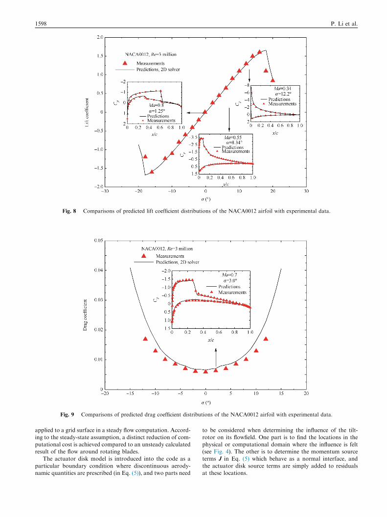
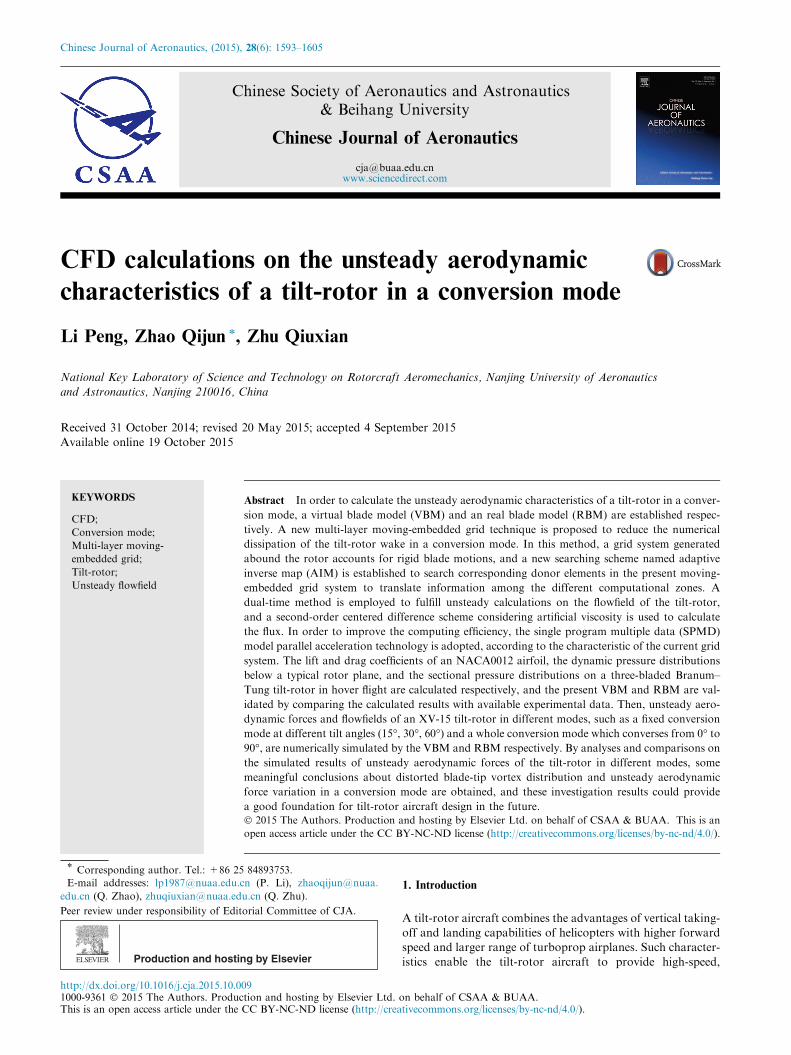
Fig. 8 Comparisons of predicted lift coefficient distributions of the NACA0012 airfoil with experimental data.
Fig. 9 Comparisons of predicted drag coefficient distributions of the NACA0012 airfoil with experimental data.
1598 P. Li et al.
applied to a grid surface in a steady flow computation. Accord-ing to the steady-state assumption, a distinct reduction of com-
putational cost is achieved compared to an unsteady calculatedresult of the flow around rotating blades.
The actuator disk model is introduced into the code as a
particular boundary condition where discontinuous aerody-namic quantities are prescribed (in Eq. (5)), and two parts need
to be considered when determining the influence of the tilt-rotor on its flowfield. One part is to find the locations in the
physical or computational domain where the influence is felt(see Fig. 4). The other is to determine the momentum sourceterms J in Eq. (5) which behave as a normal interface, and
the actuator disk source terms are simply added to residualsat these locations.

Table 1 Two-bladed typical rotor parameters.
Parameter Metric
Airfoil section NACA0012
Rotor radius (m) 0.914
Blade chord (m) 0.1
Tip Mach number 0.3285
Collective pitch angle u0(�) 11
Blade twist (�) 0
CFD calculations on the unsteady aerodynamic characteristics of a tilt-rotor in a conversion mode 1599
At first, a tiny element whose area is SD on the plane of theactuator disk is investigated, which is located at a distance of r
from the center of the tilt-rotor hub with a length of dr alongthe spanwise direction and a width of Dw along the circumfer-ential direction. Suppose that the instantaneous force acting on
the blade is dF, and the reacting force acting on the fluid ele-ment at this location is �dF and the resultant force is �NdFfor N blades. As a result, the time averaged force acting on
the surface of the grid cell is
FD ¼ � NdF
2prdrSD ð15Þ
Then, dF in the tiny element can be calculated. For a rotor ref-erence frame, the forces can be written as
b� ¼ arctan VZ
VO;
a ¼ u� b�dT ¼ dL cos b� � dD sin b�dQ ¼ �dL sinb� � dD cos b�dF ¼ �dT� dQ
8>>>>>><>>>>>>:ð16Þ
Fig. 10 Comparisons of predicted dynamic pressure distribu-
tions with experimental data.
where a is the effective angle of attack, u the local collective
angle, b� the angle of incidence, VZ the relative axial velocity,VO the relative tangential velocity, dL the lift of the airfoil, dDthe drag of the airfoil, and lift coefficient CL and drag coeffi-
cient CD can be obtained by a 2D-Reynolds averagedNavier–Stokes solver. Fig. 6 shows the flowchart about themomentum source calculation in the VBM method.
3.4. Real blade model
In current investigation, the whole flowfield is divided intothree zones which are shown in Fig. 3. The first zone covers
a small region around each blade. In this zone, the viscouseffect is modeled using a Navier–Stokes solver. The secondzone covers the first zone to reduce the dissipation of the wake
due to truncation errors and artificial viscosity presented innumerical algorithms. The third zone includes the inviscidregion away from the blade, which is usually located one ormore rotor diameters away from the rotor disk. The latter
two zones are modeled by using an Euler solver. To allowthe vortex to propagate out from the Navier–Stokes zone tothe inviscid zone without false reflections, the embedded region
between the three zones need be carefully handled.In order to improve the computational efficiency, the single
program multiple data (SPMD) model parallel acceleration
technology21 has been adopted. Careful consideration of paral-lel computing issues including load balancing and re-establishing data communication becomes critical to ensure
efficient computational performance. Spatial decompositionfor parallel processing is achieved by distributing grids amongthe processors. The grid size in this investigation is over 3.7million elements. Taking a revolution with 10800 iterations
as an example, only 3.2 h are consumed by using 5 processorsin the simulations compared to 13.4 h by a single CPU. Theresults indicate 4.2 time acceleration compared to the single
CPU implementation, and the acceleration efficiency is over80%. The numerical example shows that the parallel methodcan achieve a better parallel speedup ratio and also save the
storage efficiently. Fig. 7 illustrates the whole RBM processesin a simplified sequence flow diagram.
4. Results and discussions
The two analytical methods proposed in this work are vali-dated by comparing the calculated results of an NACA0012
airfoil under different working conditions, a two-bladed typi-cal rotor, and a three-bladed tilt-rotor in hover with availableexperimental data. In addition, full and fixed conversion casesare calculated by the VBM or RBM respectively in order to
investigate the unsteady aerodynamic characteristics of thetilt-rotor.
Table 2 Three-bladed Branum–Tung tilt-rotor parameters.
Parameter Metric
Airfoil section NACA64 series
Rotor radius (m) 0.61
Rotor solidity 0.1194
Tip Mach number 0.338
Collective pitch angle (�) 8
Blade twist (�) �32

Fig. 11 Comparisons of pressure coefficient distributions of the
Branum–Tung blade in hover with experimental data.
1600 P. Li et al.
4.1. 2D airfoil case
Simulations for the flowfield of the NACA0012 airfoil are con-ducted by the present method (simplified from a 3D RBM sol-ver), and the size of the C-type grid around the airfoil is
193� 49. Fig. 8 shows the lift coefficient CL distributionsalong the angle of attack and the airfoil surface pressure coef-ficient Cp distributions at three different positions, and Fig. 9shows the drag coefficient CD distributions along the angle
of attack and the surface pressure coefficient distribution ata fixed position. It is clearly seen from the comparisons inthe figures that the results predicted by using the proposed
2D solver agree well with the experimental data.
Fig. 12 Convergence history of thrust coefficient of the XV-15
tilt-rotor in a fixed conversion mode.
4.2. Two-bladed typical rotor
The parameters of the typical rotor22 are given in Table 1. TheVBM is validated in this numerical case, and the size of thebackground grids is 117� 121� 85. Fig. 10 shows compar-
isons between predicted dynamic pressure distributions (r/Ris the proportional position of the span direction) and experi-mental data at different axial positions below the rotor disk,which demonstrate good agreements between the calculated
results and experimental data. It shows that the proposedVBM method is effective to simulate the flowfield of the rotor.
4.3. Three-bladed Branum–Tung tilt-rotor
A tilt-rotor with three blades23 is taken as the numerical exam-ple to verify the effectiveness of the RBM, the size of the C–O
type blade grids of which is 193� 49� 65 and the size of thebackground grids is 117� 121� 85. The rotor parameters orcharacteristics are given in Table 2. Fig. 11 compares the cal-
culated pressure coefficients of the blade section along thespanwise of the blade with the experimental results, and theyagree well with each other, which indicates that the RBMmethod is capable to capture the flowfield around the tilt-
rotor blades in a hover mode.
4.4. Tilt-rotor in a conversion mode
A whole XV-15 tilt-rotor conversion case from 0� (vertical) to90� (horizontal) is used to analyze the aerodynamic effects ofunsteady movement of the tilt-rotor and the difference between
the whole and fixed conversion modes. In this case, the size ofthe C-O type blade grids is 193� 49� 65, the size of the tran-sition grids is 125� 61� 125, and the size of the background
grids is 117� 121� 85. The operating conditions of the rotorare: advance ratio l ¼ 0:15; tip Mach number Matip ¼ 0:69;
h0 ¼ 15�, and conversion time Ttilt ¼ 5 s:Because of the differences in flow conditions, the simulation
process of XV-15 in a fixed conversion mode requires about
three rotor revolutions for the force history to fully convergeto the periodic state in the RBM, as illustrated in Fig. 12,where CT is thrust coefficient. Fig. 13 gives the calculatedthrust coefficient distributions of a blade in a conversion mode
by the RBM. As clearly demonstrated in the results, the thrustdecreases gradually and smoothly with the increase of the tilt
Fig. 13 Thrust coefficient distributions of the XV-15 blade in a
conversion mode.

Fig. 14 Thrust coefficient distributions of the XV-15 tilt-rotor in
different conversion modes.
Table 3 Comparisons of CPU time between the two solvers.
Calculation case Cost time (h)
VBM RBM
A fixed conversion case 0.29 9.57
A whole conversion case 26.1 153.7
CFD calculations on the unsteady aerodynamic characteristics of a tilt-rotor in a conversion mode 1601
angle. This phenomenon is caused by the decrease of the effec-tive angle of attack due to the increase of the inflow angle.
Fig. 14 shows the thrust coefficient distributions of the tilt-rotor in different conversion modes calculated by the VBMand RBM methods respectively. The thrust variations of the
Fig. 15 Comparisons of local thrust coefficient distributions along th
and fixed conversion modes.
tilt-rotor calculated from the VBM and the RBM show a sim-ilar behavior. By the comparisons of the lift coefficient varia-tions, it can be seen that good agreements between the
calculated results by the VBM and the RBM are observed indifferent conversion modes. There is basically a slight increaseof the tilt-rotor lift coefficient in the whole conversion mode
compared to the fixed conversion mode, due to the impact ofthe tilting motion in the whole conversion mode, which is ben-eficial for keeping the produced lift of the tilt-rotor in an actual
conversion mode.In the present investigation, the developed codes are set up
on a cluster with 14 I7 (3.4 G) CPUs. The computationalresource requirements are compared between the VBM and
the stand-alone RBM in a conversion mode. The comparisonsare given in Table 3, and the simulations by the two methodsare performed in the same background grids.
For the VBM calculation in a fixed conversion mode, theconverged solution can be achieved in approximately 0.29 hon 5 processors. For the same case considered, the computa-
tion time is about 9.57 h by using the proposed RBM method.A typical calculation for the whole conversion mode conditionrequires approximately 154 h of CPU time, which needs about
50 rotor revolutions and 50 iterations for a step size of 5� in theazimuthal position to obtain a converged solution by the RBMcalculations. It is demonstrated that from the point of compu-tational efficiency, it would be better to use the VBM method
to analyze the overall performance of the tilt-rotor in thewhole conversion, instead of the RBM method.
Fig. 15 gives the calculated thrust coefficient Ma2Cn (Cn isthe normal force coefficient) distributions along the blade
e XV-15 blade spanwise on the advancing side between the whole

Fig. 16 Comparisons of vorticity magnitude and iso-vorticity contour in whole and fixed conversion flights (in the background grid).
Fig. 17 Comparisons of vorticity magnitude and iso-vorticity contour in whole and fixed conversion flights by the refined grid (in the
background grid).
1602 P. Li et al.

Fig. 18 Predicted normalization rotor thrust distributions in the fixed conversion mode.
CFD calculations on the unsteady aerodynamic characteristics of a tilt-rotor in a conversion mode 1603
spanwise at the advancing side in four different conversion
modes at 15�, 30�, 60�, and 90� tilt angles by using theRBM. Different calculated results show that majority of thrust
is generated outboard on the blade, and similar distributions
along the blade are calculated by the RBM method. However,it can be clearly seen that thrust has a slightly smaller value in

1604 P. Li et al.
the whole conversion than the fixed conversion at 15�, while areverse trend is shown in the rest majority of tilt angles. Thesedifferences are caused by effectively capturing the unsteady
aerodynamic characteristics of the tilt-rotor in the whole con-version mode by the RBM.
To illustrate the aerodynamic interference of the tilt-rotor in
the whole conversion mode, different flowfields of the XV-15tilt-rotor at three typical tilt angles in a conversion mode areshown in Fig. 16. The flowfield around the tilt-rotor blade is
captured well, which indicates the good potential of the presentmethod in calculating the unsteady aerodynamic force of therotor in a conversion mode. A stronger and distorted blade-tip wake in the whole conversion mode is obviously observed
than that of the fixed conversion mode. As the increase of thetilt angle, this phenomenon is gradually weakened, and themain reason is due to the increase of the inflow speed.
In order to capture the unsteady flowfield of the tilt-rotormore accurately at the conversion regions where the unsteadyflow characteristics change rapidly, more grid points should be
generated in the calculations. Fig. 17 gives the comparisons ofthe different flowfields calculated by the two methods using thesame refined background grids (233� 193� 169). A more
obvious wake distortion in the whole conversion mode canbe observed compared with that in the fixed mode calculatedby the RBM. It can also be seen from the figures that the vor-tex shed from the tilt-rotor is captured more clearly than that
shown in Fig. 16 at the same condition.Fig. 18 shows the rotor thrust variations of the tilt-rotor
over the whole rotor disk at different tilt angles. For the two
conversion states of tilt angles / ¼ 15� and / ¼ 30�, it is foundthat the maximum thrust is located between 90� and 270� azi-muthal angles. However, the amplitudes decrease with the
increase of the tilt angle, as shown in Fig. 16. It indicates thatthe free stream decreases the blade’s effective angle of attack,resulting in the special rotor loading distribution in this region.
With the increase of the tilt angle, thrust distributions of thetilt-rotor become gradually uniform over the whole azimuthand the thrust of the blade root increases gradually.
5. Conclusions
VBM/RBM solvers are developed in this work to predict theflowfield around a tilt-rotor in a conversion mode. The devel-
oped solvers are validated through comparing the calculatedresults with the available experimental data. The solvers arealso used to investigate the effects of different flight modes
on the tilt-rotor flowfield.
(1) A combination of the moving-embedded grid methodol-
ogy and the AIM methodology can account for the rigidblade motions in a conversion mode, and is shown to beeffective and robust in searching for the correspondingdonor elements and getting the interpolated data for
the information communication among different calcu-lation zones. The proposed multi-layer moving-embedded grid technique is capable of capturing effec-
tively the unsteady characteristics of the flowfield ofthe tilt-rotor in a conversion mode.
(2) The proposed VBM and RBM are proved to be effective
in predicting the complicated three-dimensionalunsteady flowfield of the tilt-rotor in a conversion mode
with a dual-time method. The established RBM can pro-
vide a more detailed flowfield of the tilt-rotor in a con-version mode than the VBM. Compared with theRBM, the VBM results are consistent with the RBM
results in analyzing the overall aerodynamic perfor-mance of the tilt-rotor in the whole conversion mode.From the point of computational efficiency, the VBMshows as a more attractive choice to investigate the
whole conversion mode. Meanwhile, it is evident thatthe SPMD model parallel acceleration technologyadopted in the two methods significantly increases the
computation efficiency.(3) Due to the impact of the tilting motion in the whole con-
version mode, the values of unsteady aerodynamic
forces in the whole conversion mode are basically largerthan those in the fixed conversion mode, and a strongerand distorted blade-tip wake in the whole conversionmode is formed compared to the fixed conversion mode.
All the unsteady aerodynamic phenomena diminishgradually with the increase of the tilt-angle.
Acknowledgments
The authors thank the anonymous reviewers for their criticaland constructive review of the manuscript. This study was sup-
ported by the National Natural Science Foundation of China(No. 11272150).
References
1. Maisel MD, Giulianetti DJ, Dugan DC. The history of the XV-15
rotor research aircraft: from concept to flight. Washington, D.C.:
NASA; 2000 Jan. Report No.: NASA SP-2000-4517.
2. Johnson W, Yamauchi GK, Watts ME. Designs and technology
requirements for civil heavy lift rotorcraft. AHS vertical lift
aircraft design conference. Alexandria: AHS International; 2006.
3. Yeo H, Johnson W. Performance and design investigation of
heavy lift tilt-rotor with aerodynamic interference effects. J Aircr
2009;46(4):1231–9.
4. Felker FF, Maisel MD, Betzina MD. Full-scale tilt-rotor hover
performance. J Am Helicopter Soc 1986;31(2):10–8.
5. Yamauchi GK, Wadcock AJ, Heineck JT. Surface flow visualiza-
tion on a hovering tilt rotor blade. An American Helicopter Society
technical specialists’ meeting for rotorcraft acoustics and aerody-
namics, VA. Alexandria: AHS International; 1997.
6. Lau BH, Wadcock AJ, Heineck JT. Wake visualization of a full-
scale tilt rotor in hover. An American Helicopter Society technical
specialists’ meeting for rotorcraft acoustics and aerodynamics,
VA. Alexandria: AHS International; 1997.
7. Wadcock AJ, Yamauchi GK, Driver DM. Skin friction measure-
ments on a hovering full-scale tilt rotor. J Am Helicopter Soc
1999;44(4):312–9.
8. Radhakrishnan A, Schmitz FH. Quad tilt rotor download and
power measurements in ground effect. An 24th applied aerody-
namics conference. Alexandria: AHS International; 2006.
9. Li CH, Zhang J, Xu GH. Computational analysis on tiltrotor
aerodynamic characteristics for transitional flight. Acta Aerody-
namica Sinica 2009;27(2):173–9 [Chinese].
10. Poling DR, Rosenstein H, Rajagopalan G. Use a Navier-Stokes
code in understanding tilt-rotor flowfields in hover. J Am
Helicopter Soc 1998;43(2):103–9.
11. Gupta V, Baeder J. Investigation of quad tilt-rotor aerodynamics
in forward flight using CFD. An 20th AIAA Applied Aerodynamics
Conference. Reston: AIAA; 2002.

CFD calculations on the unsteady aerodynamic characteristics of a tilt-rotor in a conversion mode 1605
12. Potsdam MA, Strawn RC. CFD simulation of tiltrotor configu-
rations in hover. An American helicopter society 58th annual
forum. Alexandria: AHS International; 2002.
13. Lee-Rausch EM, Biedron RT. Simulation of an isolated tiltrotor
in hover with an unstructured overset-grid RANS solver. An
American helicopter society 65th annual forum. Alexandria: AHS
International; 2009.
14. Wissink A, Potsdam M, Sankaran V. A coupled unstructured-
adaptive Cartesian CFD approach for hover prediction. An
American Helicopter Society 66th annual forum. Alexandria: AHS
International; 2010.
15. Potsdam M, Strawn R. CFD simulations of tiltrotor configura-
tions in hover. J Am Helicopter Soc 2005;50(1):82–94.
16. Sheng CH, Narramore JC. Computational simulation and analysis
of Bell Boeing quad tilt-rotor aero interaction. An American
Helicopter Society 64th annual forum. Alexandria: AHS Interna-
tional; 2008.
17. Zhao QJ, Xu GH, Zhao JG. Numerical simulations of the
unsteady flowfield of helicopter rotors on moving embedded grids.
Aerosp Sci Technol 2005;9(2):117–24.
18. Zhao QJ, Xu GH, Zhao JG. New hybrid method for predict-
ing the flowfields of helicopter rotors. J Aircr 2006;43(2):
132–40.
19. Ruith MR. Unstructured, multiplex rotor source model with
thrust and moment trimming – Fluent’s VBM model. An 23rd
AIAA applied aerodynamics conference. Reston: AIAA; 2005.
20. Zhang Y, Ye L, Yang S. Numerical study on flow fields and
aerodynamics of tilt rotor aircraft in conversion mode based on
embedded grid and actuator model. Chin J Aeronaut 2015;28
(1):93–102.
21. Allen CB. Parallel flow-solver and mesh motion scheme for
forward flight rotor simulation. Reston: AIAA; 2006. Report No.:
AIAA-2006-3476.
22. McKee JW, Naeseth RL. Experimental investigation of the drag
of flat plates and cylinders in the slipstream of a hovering rotor.
Washington, D.C.: Langley Aeronautical Laboratory; 1958 Apr.
Report No.: NACA-TN-4239.
23. Branum L, Tung C. Performance and pressure data from a small
model tiltrotor in hover. Washington, D.C.: AMES Research
Center; 1997 Apr. Report No.: NASA TM 110441.
Li Peng is a Ph.D. student in aircraft design at Nanjing University of
Aeronautics and Astronautics, and his research interests are helicopter
CFD, parallel computation, and flight control on tilt-rotor aircraft.
Zhao Qijun is a professor and Ph.D. advisor in the College of Aero-
space Engineering at Nanjing University of Aeronautics and Astro-
nautics, where he received his Ph.D. degree in aircraft design. His main
research interests are helicopter CFD, helicopter aerodynamics, aero-
dynamic shape design of rotor blades, active flow control on aerody-
namic characteristics of rotors, and rotor aeroacoustics.
Zhu Qiuxian is an M.E. student in aircraft design at Nanjing
University of Aeronautics and Astronautics, and her research interests
are helicopter CFD, helicopter aerodynamics, and flight control on tilt-
rotor aircraft.