unsteady aerodynamic force sensing from measured … · unsteady aerodynamic force sensing from...

Unsteady Aerodynamic Force Sensing from Measured Strain

Prepared For:

30th Congress of the International Council of the Aeronautical ScienceDaejeon, South Korea, September 25-30, 2016

Prepared By:

Chan-gi Pak, Ph.D.

Structural Dynamics Group, Aerostructures Branch (Code RS)

NASA Armstrong Flight Research Center

https://ntrs.nasa.gov/search.jsp?R=20160011960 2018-07-29T01:23:58+00:00Z

Chan-gi Pak-2/22Structural Dynamics Group

Overview Theoretical background (slides 3-9)

What the technology does (slide 3)

Previous technologies (slide 4)

Steps used to compute aerodynamic load from measured strain (slide 5)

Technical features of two-step approach: deflection (slide 6)

Technical features of new technology: velocity & acceleration (slide 7)

Technical features of expanding procedure (slide 8)

Technical features of new technology: unsteady aerodynamic loads (slide 9)

Computational validation (slides 10-21)

Structural Model & Results from Modal Analysis (slide 11)

CFL3D Model & Aeroelastic Analysis using CFL3D/NASTRAN (slide 12)

CFL3D vs. MSC/NASTRAN: deflection & velocity (slide 13)

Time Histories of Strain under Different Levels of Random White Noise (slide 14)

Time Histories of Z Deflection: SNR = 0 dB (slide 15)

Time Histories of Z Velocity: SNR = 0 dB (slide 16)

Time Histories of Z Acceleration: SNR = 0 dB (slide 17)

Time Histories of Total Induced Drag Load under Different Levels of Random White Noise (slide 18)

Time Histories of Total Spanwise Load under Different Levels of Random White Noise (slide 19)

Time Histories of Total Lift Load under Different Levels of Random White Noise (slide 20)

Updating aerodynamic forces using scaling factor (slide 21)

Conclusions (slide 22)


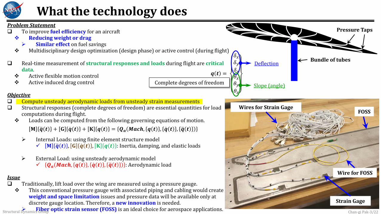
What the technology doesProblem Statement To improve fuel efficiency for an aircraft Reducing weight or drag Similar effect on fuel savings

Multidisciplinary design optimization (design phase) or active control (during flight)

Real-time measurement of structural responses and loads during flight are critical data.

Active flexible motion control Active induced drag control

Objective Compute unsteady aerodynamic loads from unsteady strain measurements Structural responses (complete degrees of freedom) are essential quantities for load

computations during flight. Loads can be computed from the following governing equations of motion.

Internal Loads: using finite element structure model 𝐌 𝒒 𝒕 , 𝐆 𝒒 𝒕 , 𝐊 𝒒 𝒕 : Inertia, damping, and elastic loads

External Load: using unsteady aerodynamic model 𝑸𝒂 𝑴𝒂𝒄𝒉, 𝒒 𝒕 , 𝒒 𝒕 , 𝒒 𝒕 : Aerodynamic load

Issue Traditionally, lift load over the wing are measured using a pressure gauge. This conventional pressure gauge with associated piping and cabling would create

weight and space limitation issues and pressure data will be available only at discrete gauge location. Therefore, a new innovation is needed.

Fiber optic strain sensor (FOSS) is an ideal choice for aerospace applications.

𝐌 𝒒 𝒕 + 𝐆 𝒒 𝒕 + 𝐊 𝒒 𝒕 = 𝑸𝒂 𝑴𝒂𝒄𝒉, 𝒒 𝒕 , 𝒒 𝒕 , 𝒒 𝒕

𝒒 𝒕 =

𝛿𝑥

𝛿𝑦

𝛿𝑧

𝜃𝑥

𝜃𝑦

𝜃𝑧

Deflection

Slope (angle)Complete degrees of freedom

Strain Gage

FOSSWires for Strain Gage

Wire for FOSS

Pressure Taps

Bundle of tubes


Previous technologies Liu, T., Barrows, D. A., Burner, A. W., and Rhew, R. D., “Determining Aerodynamic Loads Based on Optical Deformation Measurements,” AIAA Journal,

Vol.40, No.6, June 2002, pp.1105-1112

NASA LRC; Application is limited for “beam”; static deflection & aerodynamic loads

Igawa, H. et al., “Measurement of Distributed Strain and Load Identification Using 1500 mm Gauge Length FBG and Optical Frequency Domain Reflectometry,” 20th International Conference on Optical Fibre Sensors, 2009

JAXA; using inverse analysis. “Beam” application only; static deflection & loads

Richards, L. and Ko, W. , “Process for using surface strain measurements to obtain operational loads for complex structures,” US Patent #7715994, May 11, 2010

NASA AFRC; “sectional” bending moment, torsional moment, and shear force along the “beam”.

Carpenter, T.J. and Albertani, R., “Aerodynamic Load Estimation from Virtual Strain Sensors for a Pliant Membrane Wing,” AIAA Journal, Vol.53, No.8, August 2015, pp.2069-2079

Oregon State University; Aerodynamic loads are estimated from measured strain using virtual strain sensor technique.


Steps used to compute aerodynamic load from measured strain

Model independent

Model dependent

Compute unsteady aerodynamic loads

𝑸𝒂 𝒌Measure unsteady

strain

𝝐 𝒌

Expand wing deflection, velocity, &

acceleration

𝒒 𝒌

𝒒 𝒌

𝜼 𝒌 𝜼 𝒌

𝒒 𝒌

𝜼 𝒌

Compute wing deflection, velocity, &

acceleration

𝒒𝑴𝒆 𝒌

𝒒𝑴𝒆 𝒌

𝒒𝑴𝒆 𝒌

Z deflection, velocity, & acceleration along each fiber are model independent quantities

Loading analysis

Flight controller

Expansion module

Motion analyzer

Assembler module

Fiber optic strain sensor

Strain

Z deflection, velocity, &

acceleration

Deflection, velocity, &

acceleration

Drag and lift


Technical features of two-step approach : Deflection Computation First Step of two-step approach Use piecewise least-squares method to minimize noise in the

measured strain data (strain/offset): re-generate strain data Obtain cubic spline (Akima spline) function using re-generated

strain data points (assume small motion):

𝑑2𝛿𝑘

𝑑𝑠2= −𝜖𝑘(𝑠)/𝑐(𝑠)

Integrate fitted spline function to get slope data:

𝑑𝛿𝑘

𝑑𝑠= 𝜃𝑘 (𝑠)

Obtain cubic spline (Akima spline) function using computed slope data

Integrate fitted spline function to get deflection data: 𝛿𝑘(𝑠)

A measured strain is fitted using a piecewise least-squares method together with the cubic spline technique.

DeflectionCurvature

-.007

-.006

-.005

-.004

-.003

-.002

-.001

.000

.001

0 10 20 30 40 50

Cu

rva

ture

, /i

n.

Along the fiber direction, in.

Piecewise least squares curve fit boundaries

: raw data

: direct curve fit

: curve fit after piecewise LS

Extrapolated data

Z deflection along the fiber

#1

𝝐 𝒌 𝒒𝑴𝒆 𝒌

Least squares fitting with respect to spatial coordinates using piecewise polynomial functions


Time interval for least-squares curve fitting (56 time steps)

De

flecti

on

TimeSampling time (8 time steps)

for on-line parameter estimator

Step size for CFL3D &

NASTRAN computations

Updated every 8 time steps

Predict

deflections

From curve fitting

From ARMA & on-line

parameter estimator

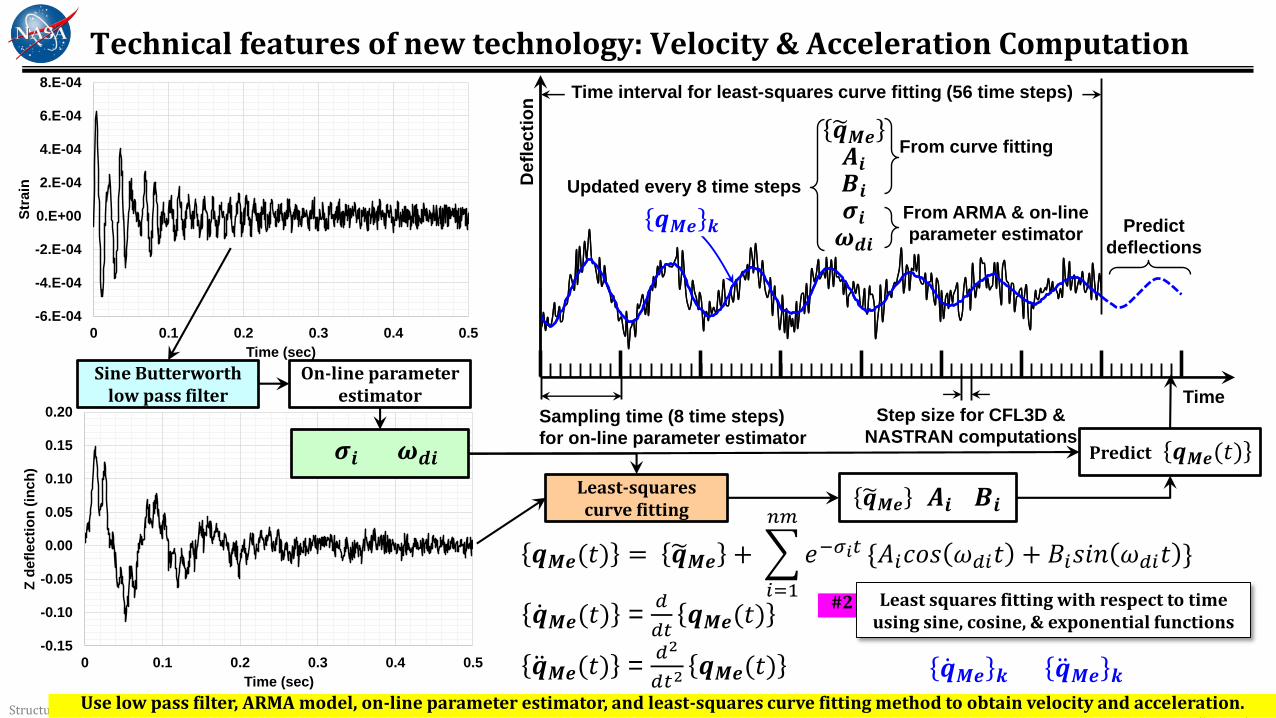
Technical features of new technology: Velocity & Acceleration Computation

𝒒𝑴𝒆(𝑡) = 𝒒𝑴𝒆 +

𝑖=1

𝑛𝑚

𝑒−𝜎𝑖𝑡 {𝐴𝑖𝑐𝑜𝑠 𝜔𝑑𝑖𝑡 + 𝐵𝑖𝑠𝑖𝑛 𝜔𝑑𝑖𝑡 }

-6.E-04

-4.E-04

-2.E-04

0.E+00

2.E-04

4.E-04

6.E-04

8.E-04

0 0.1 0.2 0.3 0.4 0.5

Str

ain

Time (sec)

Sine Butterworth low pass filter

On-line parameter estimator

-0.15

-0.10

-0.05

0.00

0.05

0.10

0.15

0.20

0 0.1 0.2 0.3 0.4 0.5

Z d

efl

ec

tio

n (

inc

h)

Time (sec)

Least-squares curve fitting

Predict

𝑨𝒊 𝑩𝒊 𝒒𝑴𝒆

𝝈𝒊 𝝎𝒅𝒊 𝒒𝑴𝒆(𝑡)

𝒒𝑴𝒆(𝑡) = 𝑑

𝑑𝑡𝒒𝑴𝒆(𝑡)

𝒒𝑴𝒆(𝑡) = 𝑑2

𝑑𝑡2 𝒒𝑴𝒆(𝑡) 𝒒𝑴𝒆 𝒌 𝒒𝑴𝒆 𝒌

#2

Use low pass filter, ARMA model, on-line parameter estimator, and least-squares curve fitting method to obtain velocity and acceleration.

Least squares fitting with respect to time using sine, cosine, & exponential functions


Technical features of expanding procedure Second step of two step approach: Based on General Transformation

Definition of the generalized coordinates vector 𝒒 𝒌 and the othonormalizedcoordinates vector 𝜼 𝒌 at discrete time k

For all model reduction/expansion techniques, there is a relationship between the master (measured or tested) degrees of freedom and the slave (deleted or omitted) degrees of freedom which can be written in general terms as

Changing master DOF at discrete time k 𝒒𝑴 𝒌 to the corresponding measured values 𝒒𝑴𝒆 𝒌

Expansion of displacement using SEREP: kinds of least-squares surface fitting; most accurate reduction-expansion technique 𝒒𝑴𝒆 𝒌: master DOF at discrete time k; deflection along the fiber “computed

from the first step”

𝒒𝑴 𝒌 = 𝚽𝑴 𝚽𝑴𝑻 𝚽𝑴

−𝟏𝚽𝑴

𝑻 𝒒𝑴𝒆 𝒌: smoothed master DOF

𝒒𝑺 𝒌 = 𝚽𝑺 𝚽𝑴𝑻 𝚽𝑴

−𝟏𝚽𝑴

𝑻 𝒒𝑴𝒆 𝒌: deflection and slope all over the

structure

𝒒 𝒌 =𝒒𝑴

𝒒𝑺 𝒌= 𝚽 𝜼 𝒌 =

𝚽𝑴

𝚽𝑺𝜼 𝒌

𝒒𝑴 𝒌 = 𝚽𝑴 𝜼 𝒌 𝒒𝑺 𝒌 = 𝚽𝑺 𝜼 𝒌

𝒒𝑴𝒆 𝒌 = 𝚽𝑴 𝜼 𝒌

𝜼 𝒌 = 𝚽𝑴𝑻 𝚽𝑴

−1𝚽𝑴

𝑻 𝒒𝑴𝒆 𝒌

𝚽𝑴𝑻 𝒒𝑴𝒆 𝒌 = 𝚽𝑴

𝑻 𝚽𝑴 𝜼 𝒌

Z motion along the fiber


−1𝚽𝑴



−1𝚽𝑴



−1𝚽𝑴


𝒒 𝒌 =𝚽𝑴

𝚽𝑺𝜼 𝒌

𝒒 𝒌 =𝚽𝑴

𝚽𝑺 𝜼 𝒌

𝒒 𝒌 =𝚽𝑴

𝚽𝑺 𝜼 𝒌

System Equivalent Reduction and Expansion Process

#3

𝒒𝑴𝒆 𝒌 𝒒𝑴 𝒌 𝒒𝑺 𝒌

Least-squares “surface” fitting using basis functions


Flow

Lift from linear panel code

aerodynamic model

X

Y

Z

Technical features of New Technology: Unsteady Aerodynamic Loads

Rational function approximation: Select Roger’s Approximation

Time marching algorithm:


−1𝚽𝑴



−1𝚽𝑴



−1𝚽𝑴


𝒙 𝒌 = 𝐄 𝒙 𝒌−1 + 𝛉 𝐁 𝜼 𝒌 + 𝜼 𝒌−1

2

𝑵 𝒌 = 𝑞𝐷 𝐃0 𝜼 𝒌 + 𝐃1 𝜼 𝒌 + 𝐃2 𝜼 𝒌 + 𝐂 𝒙 𝒌

𝐄 = 𝑒 𝐀 𝑇𝑎 𝛉 = 0

𝑇𝑎

𝑒 𝐀 (𝑇𝑎−𝜏 𝑑𝜏 𝐀 =

−Ω1𝐈 0 … 00 −Ω2𝐈 … 0⋮0

⋮0

⋱ ⋮… −ΩLT𝐈

𝐁 =

𝐈𝐈⋮𝐈

𝐂 = [𝐂1 𝐂2 …𝐂𝑳𝑻 𝒙 𝒌 =

𝒙1

𝒙2

⋮𝒙𝐿𝑇 𝑘

𝐀 𝑠 = 𝐃0 + 𝑠 𝐃1 + 𝑠2 𝐃2 +

𝑗=1

𝐿𝑇𝑠 𝐂𝑗

𝑠 + Ωj

Modal Aerodynamic Influence Coefficient Matrix

𝑸𝒂 𝒌

A rectangular matrix 𝚽 𝑻 can be inverted using a singular value decomposition technique.

Lift

Drag

normal

Lift

Drag

normal

Flow

Side view of the unsteady wing motion

Flow

𝑸𝒂 𝒌 = 𝚽 𝑻 −1𝑵 𝒌

𝚽 𝑻 𝑸𝒂 𝒌 = 𝑵 𝒌

𝐌 𝒒 𝒕 + 𝐆 𝒒 𝒕 + 𝐊 𝒒 𝒕 = 𝑸𝒂(𝒕)

𝑠2 𝐌 𝚽 )𝜼(𝑠 + 𝑠 𝐆 𝚽 )𝜼(𝑠 + 𝐊 𝚽 )𝜼(𝑠 = 𝑸𝒂(𝑠)

𝑠2 𝚽 𝑻 𝐌 𝚽 )𝜼(𝑠 + 𝑠 𝚽 𝑻 𝐆 𝚽 )𝜼(𝑠 + 𝚽 𝑻 𝐊 𝚽 )𝜼(𝑠= 𝚽 𝑻 𝑸𝒂(𝑠) = )𝑵(𝑠 = 𝑞𝐷 𝐀 𝑠 )𝜼(𝑠

Computational Validation

Cantilevered rectangular wing model


Fibers 1 & 2

11.5 inch4

.56

in

ch

Fiber Optic Strain Sensors: 3(upper)+ 3(lower)

X

Y A

A

Fibers 3 & 4

Fibers 5 & 6

Structural Model & Results from Modal Analysis

Fibers

Plate elements

Strain plot element

Rigid element

Z

X

Configuration of a wind tunnel test article Has aluminum insert (thickness = 0.065 in ) covered with 6% circular arc cross-sectional shape

(plastic foam)

lumped mass weight are computed based on 6% circular-arc cross sectional shape.

Use structural dynamic model tuning technique

Chan-gi Pak and Samson Truong, “Creating a Test-Validated Finite-Element Model of the X-56A Aircraft Structure,” Journal of Aircraft, Vol. 52, No. 5, pp. 1644-1667, 2015. doi: http://arc.aiaa.org/doi/abs/10.2514/1.C033043

300 beam elements for fictitious FOSS (50 per each fiber). Zero stiffness and zero weight. Modal analysis

NASTRAN sol. 103

Mode 1 Mode 2 Mode 3

Measured and computed natural frequencies

Mode Measured (Hz) Computed (Hz) % Error

1 14.29 14.29 0.0

2 80.41 80.17 -0.3

3 89.80 89.04 -0.8

0.065” aluminum insert Flexible plastic foam

6% Circular arcA-A

http://arc.aiaa.org/doi/abs/10.2514/1.C033044


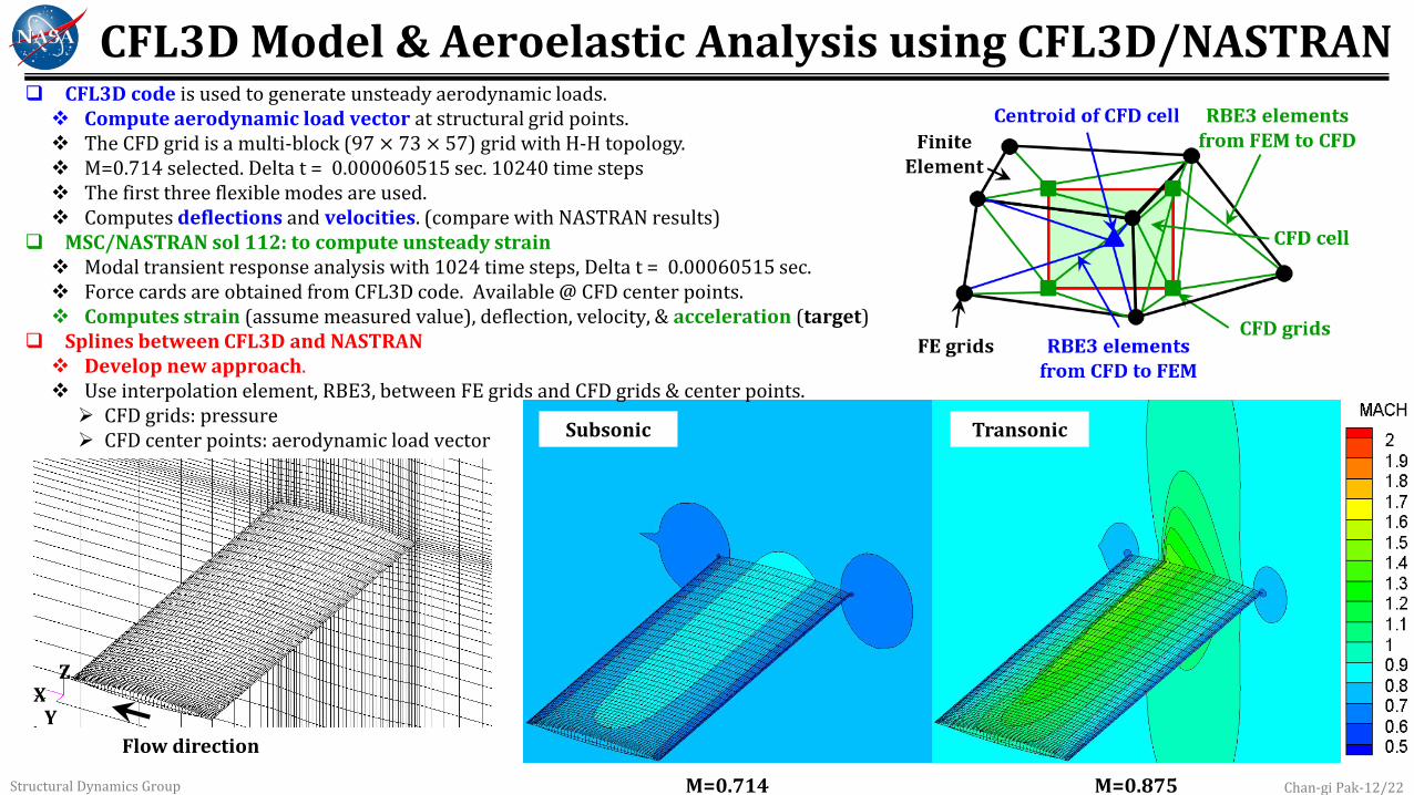
CFL3D Model & Aeroelastic Analysis using CFL3D/NASTRAN

Flow direction

XY

Z

M=0.714 M=0.875

CFL3D code is used to generate unsteady aerodynamic loads. Compute aerodynamic load vector at structural grid points. The CFD grid is a multi-block (97 × 73 × 57) grid with H-H topology. M=0.714 selected. Delta t = 0.000060515 sec. 10240 time steps The first three flexible modes are used. Computes deflections and velocities. (compare with NASTRAN results)

MSC/NASTRAN sol 112: to compute unsteady strain Modal transient response analysis with 1024 time steps, Delta t = 0.00060515 sec. Force cards are obtained from CFL3D code. Available @ CFD center points. Computes strain (assume measured value), deflection, velocity, & acceleration (target)

Splines between CFL3D and NASTRAN Develop new approach. Use interpolation element, RBE3, between FE grids and CFD grids & center points. CFD grids: pressure CFD center points: aerodynamic load vector Subsonic Transonic


CFL3D vs. NASTRAN: deflection & velocity

qd = 1.455

(a) Deflection

-0.80

-0.60

-0.40

-0.20

0.00

0.20

0.40

0 0.1 0.2 0.3 0.4 0.5 0.6

Z d

efl

ecti

on

(in

ch

)

Time (sec)

: CFL3D

: NASTRAN

(b) Velocity

-100

-80

-60

-40

-20

0

20

40

60

80

100

0 0.1 0.2 0.3 0.4 0.5 0.6

Z v

elo

cit

y (

inch

/sec)

Time (sec)

: CFL3D

: NASTRAN

qdf = 1.4561: Dynamic pressure for wing flutter condition


Time Histories of Strain under Different Levels of Random White Noise

(a) Without noise

-1.5E-3

-1.0E-3

-5.0E-4

0.0E+0

5.0E-4

1.0E-3

1.5E-3

0 0.1 0.2 0.3 0.4 0.5 0.6

Str

ain

Time (sec)

-1.5E-3

-1.0E-3

-5.0E-4

0.0E+0

5.0E-4

1.0E-3

1.5E-3

0 0.1 0.2 0.3 0.4 0.5 0.6

Str

ain

Time (sec)

(c) SNR = 6 dB

-1.5E-3

-1.0E-3

-5.0E-4

0.0E+0

5.0E-4

1.0E-3

1.5E-3

0 0.1 0.2 0.3 0.4 0.5 0.6

Str

ain

Time (sec)

(d) SNR = 0 dB

Rms = 3.28 E-4

Strain is measured at the leading-edge of wing root section (upper surface).

𝑆𝑁𝑅 ≡ 20 × 𝑙𝑜𝑔10𝜖𝑟𝑚𝑠

𝑛𝑟𝑚𝑠

𝜖𝑟𝑚𝑠 root-mean-squared level of strain

𝑛𝑟𝑚𝑠 root-mean-squared level of noise

SNR value is correct near 0.33 sec.

𝐿𝑆𝑁𝑅 ≡ 20 × 𝑙𝑜𝑔10𝜖𝑚𝑎𝑥

𝑛𝑟𝑚𝑠

𝜖𝑚𝑎𝑥 local maximum strain

𝑛𝑟𝑚𝑠 root-mean-squared level of noise

LSNR @ 0.035 sec

20log10(8.97/3.28) = 8.74 dB

LSNR @ 0.24 sec

20log10(3.95/3.28) = 1.61 dB

LSNR @ 0.33 sec

20log10(3.28/3.28) = 0 dB

LSNR @ 0.59 sec

20log10(1.06/3.28) = -9.83 dB

8.97 E-4

1.06 E-4

3.95 E-4

-1.5E-3

-1.0E-3

-5.0E-4

0.0E+0

5.0E-4

1.0E-3

1.5E-3

0 0.1 0.2 0.3 0.4 0.5 0.6

Str

ain

Time (sec)

1.6 dB -9.8 dB8.7 dB 0 dB

(b) SNR = 10 dB

3.28 E-4


Time Histories of Z Deflection: SNR = 0 dB

Z deflection is computed at the leading-edge of wing tip section (upper surface). Time interval: 0 – 0.2414 sec Learning period for on-line parameter estimator. Effect of piecewise least squares method can be observed. (first step of two step approach)

Time interval: 0.2141 sec – 0.6 sec Least-squares curve fitting method is on. Working even with “SNR = 0 dB”

Effect of SEREP transformation can be observed. SEREP transformation is a kind of least-squares surface fitting approach. Noise in the signal after the first step of the two step approach is further filtered using SEREP transformation.


𝑖=1

𝑛𝑚



−1𝚽𝑴

𝑻 𝒒𝑴𝒆 𝒌𝒒 𝒌 =𝚽𝑴

𝚽𝑺𝜼 𝒌

-1

-0.5

0

0.5

0 0.1 0.2 0.3 0.4 0.5 0.6

Z d

efl

ec

tio

n (

inc

h)

Time (sec)

: NASTRAN: Before SEREP: After SEREP0.2414

Least-squares

curve fitting onLeast-squares

curve fitting off

1.6 dB -9.8 dB8.7 dB 0 dB

Piecewise least-squares method#1

Piecewise least-squares method#1

#2

#3Learning period


Time Histories of Z Velocity: SNR = 0 dB

Z velocity is computed at the leading-edge of wing tip section (upper surface).

Time interval: 0 – 0.2414 sec

Learning period for on-line parameter estimator.

Velocities are not computed during this period.

Time interval: 0.2141 sec – 0.6 sec

Least-squares curve fitting method is on.

Working even with “SNR = 0 dB”


𝑖=1

𝑛𝑚


𝒒𝑴𝒆(𝑡) = 𝑑

𝑑𝑡𝒒𝑴𝒆(𝑡)


−1𝚽𝑴

𝑻 𝒒𝑴𝒆 𝒌 𝒒 𝒌 =𝚽𝑴

𝚽𝑺 𝜼 𝒌

-100

-80

-60

-40

-20

0

20

40

60

80

100

0 0.1 0.2 0.3 0.4 0.5 0.6

Z v

elo

cit

y (

inch

/sec)

Time (sec)

1.6 dB

-9.8 dB

8.7 dB0 dB

: NASTRAN: Before SEREP: After SEREP

Learning period0.2414


Z acceleration is computed at the leading-edge of wing tip section (upper surface).



Accelerations are not computed during this period.




Time Histories of Z Acceleration: SNR = 0 dB


𝑖=1

𝑛𝑚


𝒒𝑴𝒆(𝑡) = 𝑑2

𝑑𝑡2 𝒒𝑴𝒆(𝑡)


−1𝚽𝑴

𝑻 𝒒𝑴𝒆 𝒌 𝒒 𝒌 =𝚽𝑴

𝚽𝑺 𝜼 𝒌

-3.E+4

-2.E+4

-1.E+4

0.E+0

1.E+4

2.E+4

3.E+4

0 0.1 0.2 0.3 0.4 0.5 0.6

Z a

cc

ele

rati

on

(in

ch

/se

c^

2)

Time (sec)

: NASTRAN: Before SEREP: After SEREP

1.6 dB

-9.8 dB

8.7 dB 0 dB

Learning period0.2414


Time Histories of Total Induced Drag Load under Different Levels of Random White Noise



Load computations are based on wing deflection only.



Big difference before and after the proposed method is on.


CFL3D calculation

Subtracted 0.0353 (thickness effect)


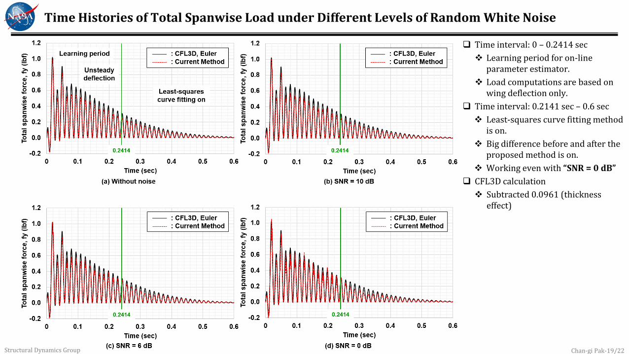
Time Histories of Total Spanwise Load under Different Levels of Random White Noise








CFL3D calculation



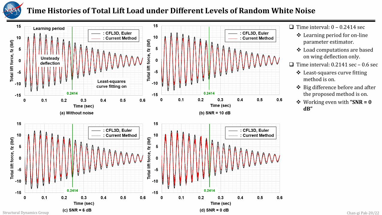
Time Histories of Total Lift Load under Different Levels of Random White Noise









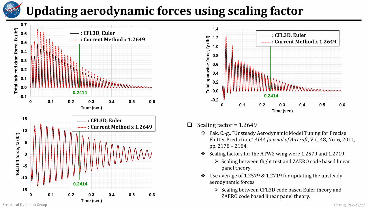
Updating aerodynamic forces using scaling factor

Scaling factor = 1.2649

Pak, C.-g., “Unsteady Aerodynamic Model Tuning for Precise Flutter Prediction,” AIAA Journal of Aircraft, Vol. 48, No. 6, 2011, pp. 2178 – 2184.

Scaling factors for the ATW2 wing were 1.2579 and 1.2719.

Scaling between flight test and ZAERO code based linear panel theory.

Use average of 1.2579 & 1.2719 for updating the unsteady aerodynamic forces.

Scaling between CFL3D code based Euler theory and ZAERO code based linear panel theory.

0.2414

: CFL3D, Euler: Current Method x 1.2649

0.2414


0.2414



Conclusions Unsteady aerodynamic loads are computed using simulated measured strain data.

Unsteady structural deflections are computed using the two-step approach.

Unsteady velocities and accelerations are computed using the ARMA model, on-line parameter estimator, low pass filter, and a least-squares curve fitting method together with an analytical derivatives with respect to time.

The deflections, velocities, and accelerations at each sensor location is independent of structural and aerodynamic models.

The distributed strain data together with the current proposed approaches can be used as a distributed deflection, velocity, and acceleration sensors.

Induced drag loads, spanwise loads, and lift loads are obtained from the orthonormalized deflection, velocity, and acceleration together with the following approaches.

The modal AIC matrices are fitted in Laplace-domain using Roger’s approximation.

Laplace-domain aerodynamics are converted to the time-domain using time-marching algorithm.

Orthonormalized aerodynamic load vectors are transformed to the general coordinates using pseudo matrix inversion based on singular value decomposition.

Normal vectors to the oscillating wing surface are used to compute drag and spanwise loads.

An active induced drag control system can be designed using these two computed aerodynamic loads, induced drag and lift, to improve the fuel efficiency of an aircraft.

Interpolation elements (RBE3 in MSC/NASTRAN terminology) between structural FE grids and the CFD grids are successfully incorporated with the unsteady aeroelastic computation scheme.

The numerical issues often associated with the Harder and Desmarais surface splines technique are bypassed through the use of the current technique with RBE3 elements.

The deflection, velocity, and acceleration computation based on the proposed least-squares curve fitting method are validated with respect to the unsteady strain with SNR of 10dB, 6dB, & 0dB (LSNR of 8.7dB to -9.8dB).

The most critical technology for the success of the proposed approach is the robust on-line parameter estimator since the least-squares curve fitting method depends heavily on aeroelastic system frequencies and damping factors.

Questions ?Unsteady Strain

Unsteady Motion

Unsteady Aerodynamic Loads

Loading analysis

Flight controller

Expansion module

Motion analyzer

Assembler module

Fiber optic strain sensor

Strain

Z deflection, velocity, &

acceleration

Deflection, velocity, &

acceleration

Drag and lift


-1

-0.5

0

0.5

0 0.1 0.2 0.3 0.4 0.5 0.6

Z d

efl

ec

tio

n (

inc

h)

Time (sec)

: NASTRAN: Current Method

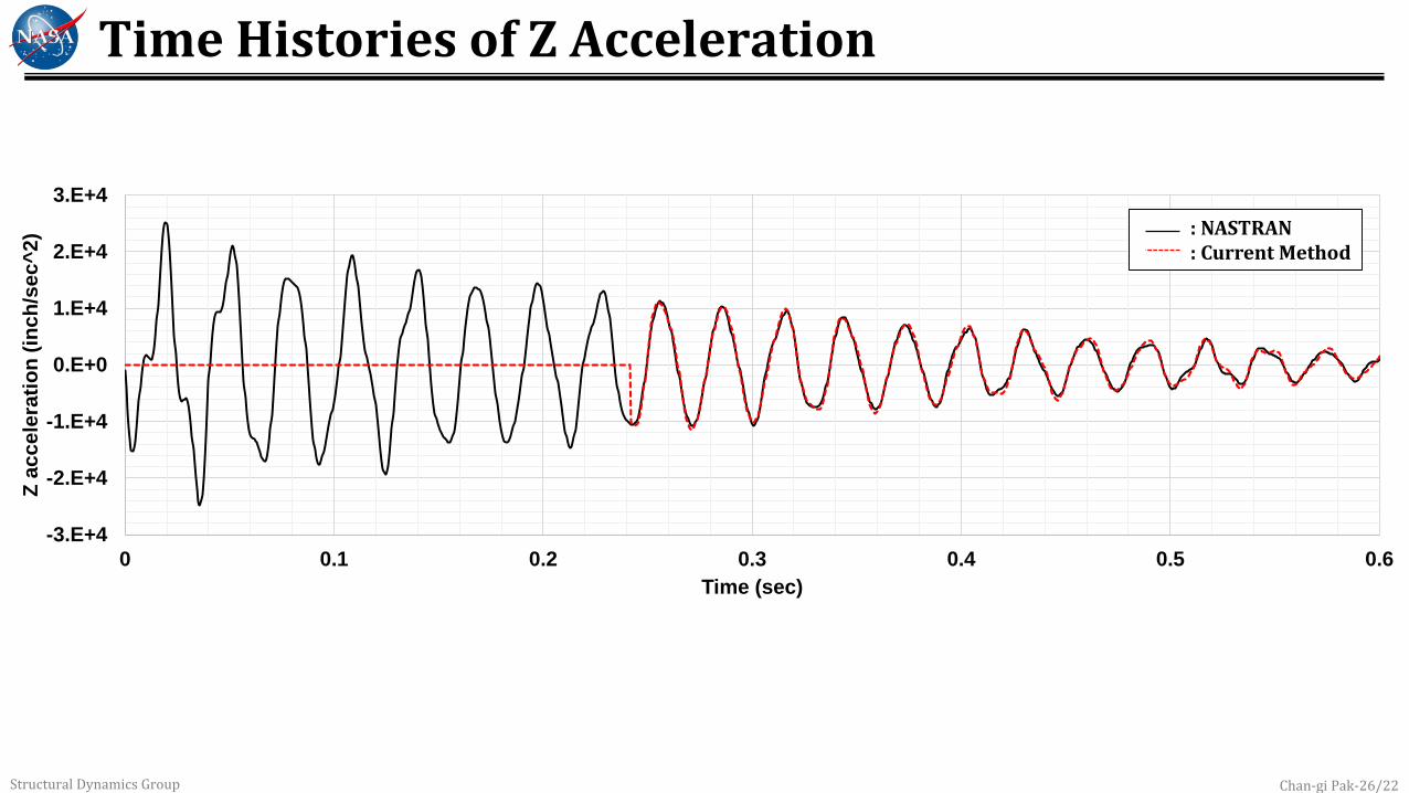
Time Histories of Z Deflection


-100

-80

-60

-40

-20

0

20

40

60

80

100

0 0.1 0.2 0.3 0.4 0.5 0.6

Z v

elo

cit

y (

inc

h/s

ec

)

Time (sec)


Time Histories of Z Velocity


-3.E+4

-2.E+4

-1.E+4

0.E+0

1.E+4

2.E+4

3.E+4

0 0.1 0.2 0.3 0.4 0.5 0.6

Z a

cc

ele

rati

on

(in

ch

/se

c^

2)

Time (sec)


Time Histories of Z Acceleration


-1.5E-3

-1.0E-3

-5.0E-4

0.0E+0

5.0E-4

1.0E-3

1.5E-3

0 0.1 0.2 0.3 0.4 0.5 0.6

Str

ain

Time (sec)

8.7 dB1.6 dB 0 dB -9.8 dB

Time Histories of Strain under 0 dB Random White Noise


-0.1

0.0

0.1

0.2

0.3

0.4

0.5

0.6

0 0.1 0.2 0.3 0.4 0.5 0.6

To

tal in

du

ced

dra

g lo

ad

, fx

(lb

f)

Time (sec)

0.2414

Time Histories of Total Induced Drag Load under 0 dB Random White Noise

: CFL3D, Euler: Current Method

1.6 dB

-9.8 dB

8.7 dB

0 dB

CFL3D calculation


Least-squares

curve fitting on

Least-squares

curve fitting off

Unsteady

deflection

Learning

period


0

20

40

60

80

100

120

0 20 40 60 80 100

Mag

nit

ud

e o

f d

efl

ecti

on

Frequency (Hz)

Aeroelastic System Frequencies From AIC computations

0 Hz

4.006Hz

10.02Hz

23.37Hz

53.42Hz

86.80Hz

173.6Hz

Aerodynamic lag terms

11.81Hz

47.22Hz

106.2Hz

188.9Hz

0

10

20

30

40

50

60

70

80

90

100

0 20 40 60 80 100

Ma

gn

itu

de

of

ind

uc

ed

dra

g lo

ad

Frequency (Hz)

0

20

40

60

80

100

120

0 20 40 60 80 100

Ma

gn

itu

de

of

sp

an

wis

e lo

ad

Frequency (Hz)

0

500

1000

1500

2000

2500

3000

0 20 40 60 80 100

Ma

gn

itu

de

of

lift

lo

ad

Frequency (Hz)

Mode Natural frequency (Hz)

1 14.29

2 80.17

3 89.04

33.74 Hz

33.89 Hz

67.71 Hz

67.61 Hz

0

2

4

6

8

10

12

0 10 20 30 40 50 60 70 80 90 100

Ma

gn

itu

de

Frequency (Hz)

qd = 1.455 qd = .7191


Roger’s Approximation

-15000

-10000

-5000

0

-1000 -500 0 500 1000 1500

Imag

inary

part

of

AIC

(1,1

)

Real part of AIC(1,1)

1 = 0.0

2 = 0.006

3 = 0.015

4 = 0.035

5 = 0.08

6 = 0.13

7 = 0.26

: AIC data

: RFA

Chan-gi Pak-31/22Structural Dynamics Group On-line parameter estimator is applied to the unsteady strain data

On-line parameter estimation with and without noise

-1

-0.8

-0.6

-0.4

-0.2

0

0.2

0.4

0.6

0.8

1

0.0 0.1 0.2 0.3 0.4 0.5

AR

MA

co

eff

icie

nts

Time (sec)

0.2414

-1

-0.8

-0.6

-0.4

-0.2

0

0.2

0.4

0.6

0.8

1

0.0 0.1 0.2 0.3 0.4 0.5

AR

MA

co

eff

icie

nts

Time (sec)

0.24140

10

20

30

40

50

60

70

80

90

100

0.0 0.1 0.2 0.3 0.4 0.5

Fre

qu

en

cy (

Hz)

Time (sec)

0.2414

-30

-25

-20

-15

-10

-5

0

5

10

0.0 0.1 0.2 0.3 0.4 0.5

Dam

pin

g f

acto

r

Time (sec)

0.2414 0

2

4

6

8

10

12

0 10 20 30 40 50 60 70 80 90 100

Ma

gn

itu

de

Frequency (Hz)

With noise, SNR=10dB

Without noise With noise, SNR=10dBWithout noise

First three damped aeroelastic frequencies

Mode

Without noiseWith noise,

SNR=10dB

FFT

(Hz)

On-line parameter estimator

Damp.

factor

Freq.

(Hz)

Damp.

factor

Freq.

(Hz)

1 13.81 -10.02 13.88 -11.11 14.12

2 63.15 -25.46 62.73 -25.92 62.62

3 89.82 -4.187 89.44 -5.740 88.74

400 steps

900 steps

𝑆𝑁𝑅 ≡ 20 × 𝑙𝑜𝑔10𝜖𝑚𝑎𝑥

𝑛𝑟𝑚𝑠

𝜖𝑚𝑎𝑥 maximum unsteady strain after 0.1 second.

𝑛𝑟𝑚𝑠 root-mean-squared level of noise.

unsteady aerodynamic force sensing from measured … · unsteady aerodynamic force sensing from...

Documents