improving an open source geocoding server - lund...
TRANSCRIPT

Imp
rovin
g a
n o
pe
n so
urce g
eo
cod
ing
serve
r
Department of Electrical and Information Technology, Faculty of Engineering, LTH, Lund University, February 2015.
Improving an open source geocoding server
Víctor García
Series of Master’s thesesDepartment of Electrical and Information Technology
LU/LTH-EIT 2015-430
http://www.eit.lth.se
Vícto
r García
Master’s Thesis

Master’s Thesis
Improving an open source geocoding
server
By
Víctor García
Department of Electrical and Information Technology
Faculty of Engineering, LTH, Lund University
SE-221 00 Lund, Sweden

2
Abstract
A common problem in geocoding is that the postal addresses as requested by
the user differ from the addresses as described in the database. The online,
open source geocoder called Nominatim is one of the most used geocoders
nowadays. However, this geocoder lacks the interactivity that most of the
online geocoders already offer. The Nominatim geocoder provides no
feedback to the user while typing addresses. Also, the geocoder cannot deal
with any misspelling errors introduced by the user in the requested address.
This thesis is about extending the functionality of the Nominatim geocoder
to provide fuzzy search and autocomplete features. In this work I propose a
new index and search strategy for the OpenStreetMap reference dataset.
Also, I extend the search algorithm to geocode new address types such as
street intersections. Both the original Nominatim geocoder and the proposed
solution are compared using metrics such as the precision of the results,
match rate and keystrokes saved by the autocomplete feature. The test
addresses used in this work are a subset selected among the Swedish
addresses available in the OpenStreetMap data set.
The results show that the proposed geocoder performs better when compared
to the original Nominatim geocoder. In the proposed geocoder, the users get
address suggestions as they type, adding interactivity to the original
geocoder. Also, the proposed geocoder is able to find the right address in the
presence of errors in the user query with a match rate of 98%.

3
Popular science article
The demand of geospatial information is increasing during the last years.
There are more and more mobile applications and services that require from
the users to enter some information about where they are, or the address of
the place they want to find for example. The systems that convert postal
addresses or place descriptions into coordinates are called geocoders. How
good or bad a geocoder is not only depends on the information the geocoder
contains, but also on how easy is for the users to find the desired addresses.
There are many well-known web sites that we use in our everyday life to find
the location of an address. For example sites like Google Maps, Bing Maps
or Yahoo Maps are accessed by millions of users every day to use such
services. Among the main features of the mentioned geocoders are the ability
to predict the address the user is writing in the search box, and sometimes
even to correct any misspellings introduced by the user. To make it more
complicated, the predictions and error corrections these systems perform are
done in real time. The owners of these address search engines usually impose
some restrictions on the number of addresses a user is allowed to search
monthly, above which the user needs to pay a fee in order to keep using the
system. This limit is usually high enough for the end user, but it might not be
enough for the software developers that want to use geospatial data in their
products.
There is a free alternative to the address search engines mentioned above
called Nominatim. Nominatim is an open source project whose purpose is to
search addresses among the OpenStreetMap dataset. OpenStreetMap is a
collaborative project that tries to map places in the real world into
coordinates. The main drawback of Nominatim is that the usability is not as
good as the competitors. Nominatim is unable to find addresses that are not
correctly spelled, neither predicts the user needs. In order for this address
search engine to be among the most used the prediction and error correction
features need to be added.
In this thesis work I extend the search algorithms of Nominatim to add the
functionality mentioned above. The address search engine proposed in this
thesis offers a free and open source alternative to users and systems that
require access to geospatial data without restrictions.

4
Resumen:
Alumno: Víctor García Paje
Título: Mejora de un sistema de geolocalización de código libre
Tutor: Maria Kihl
Institución: Lund Tekniska Högskola, Lund, Suecia
Fecha de defensa del proyecto: 26-01-2015
La demanda de información geoespacial está aumentando en los últimos
años. Cada vez existen más aplicaciones y servicios móviles que requieren
de los usuarios introducir información acerca de dónde están, o la dirección
del lugar que quieren encontrar por ejemplo. Los sistemas que convierten las
direcciones postales a coordenadas y viceversa se llaman geocodificadores.
Cómo de bueno o malo es un geocodificador no sólo depende de la
información que el geocodificador contiene, sino también en lo fácil que es
para los usuarios encontrar las direcciones deseadas.
Existen muchos sitios web conocidos que utilizamos en nuestra vida
cotidiana para encontrar la ubicación de una dirección. Por ejemplo, sitios
como Google Maps, Bing Maps o Yahoo Maps son accedidos por millones
de usuarios cada día. Entre las principales características de los
geocodificadores se encuentran la capacidad de predecir la dirección que el
usuario está escribiendo en el campo de búsqueda y, a veces incluso de
corregir los errores ortográficos introducidos por el usuario. Para hacerlo más
complicado, las predicciones y las correcciones de errores en estos sistemas
se realizan en tiempo real. Los propietarios de estos motores de búsqueda de
direcciones generalmente imponen restricciones en la cantidad de
direcciones que se permite buscar a un usuario en un plazo de tiempo,
generalmente un mes, por encima del cual el usuario tiene que pagar una
cuota para poder seguir usando el sistema. Este límite suele ser lo
suficientemente alto para el usuario final, pero tal vez no sea suficiente para
desarrolladores de software que quieran utilizar datos geoespaciales en sus
productos.
Hay una alternativa de código libre a los motores de búsqueda de direcciones
mencionadas anteriormente llamado Nominatim. Nominatim es un proyecto
de código libre cuyo propósito es buscar direcciones entre el conjunto de
datos de OpenStreetMap. OpenStreetMap es un proyecto colaborativo que
intenta asignar lugares en el mundo real a coordenadas. El principal
inconveniente de Nominatim es que la usabilidad del sistema no es tan buena

5
como la de los competidores. Nominatim no puede encontrar las direcciones
que no están escritas correctamente, ni predice las búsquedas de los usuarios.
Para que este motor de búsqueda de direcciones pueda estar entre los más
utilizados se deben agregar las funciones de corrección de errores y de
predicción.
En este proyecto mejoro los algoritmos de búsqueda de Nominatim para
añadir la funcionalidad mencionada anteriormente. El principal objetivo del
proyecto consiste en estudiar técnicas de corrección de errores y predicción
de búsquedas. Posteriormente diseñar un sistema de indexado para realizar
estas funciones de forma eficiente y en tiempo real. Por último, implementar
el sistema y testearlo para ser comparado con el sistema original llamado
Nominatim. El motor de búsqueda de direcciones propuesto en esta tesis
ofrece una alternativa de código libre a usuarios y sistemas que requieren
acceso a datos geoespaciales sin restricciones.

6
Acknowledgements This Master’s thesis would not exist without the invaluable support and
guidance of my supervisor and examiner Dr. Maria kihl. Also, I would like
to thank to my family for the not to be underestimated mental support.
Víctor García Paje

7
Table of Contents Abstract ......................................................................................................... 2
Acknowledgements ....................................................................................... 6
Table of Contents .......................................................................................... 7
1 Introduction ........................................................................................... 9
1.1 Introduction ................................................................................... 9
1.2 Research questions ...................................................................... 11
1.3 Methodology ............................................................................... 12
1.4 Goals ........................................................................................... 12
1.5 Limitations .................................................................................. 13
1.6 Outline of the thesis .................................................................... 13
2 Relevant work ..................................................................................... 14
2.1 Geocoding ................................................................................... 14
2.1.1 Sources of error in the geocoding process ........................... 16
2.2 Information retrieval ................................................................... 17
2.2.1 Fundamentals of prefix and fuzzy search ............................ 23
2.2.2 Document Similarity and TF-IDF ....................................... 25
2.2.3 Text indexing ....................................................................... 27
2.3 Evaluation metrics....................................................................... 28
3 OpenStreetMap and Nominatim ......................................................... 31
3.1 OpenStreetMap ........................................................................... 31
3.1.1 OSM data model .................................................................. 31
3.2 Nominatim .................................................................................. 34
3.2.1 Usage and statistics ............................................................. 35
3.2.2 Database overview .............................................................. 36
3.2.3 Processing OSM data .......................................................... 37
3.2.3.1 Processing feature names ................................................ 37
3.2.3.2 OSM Administrative boundaries .................................... 39
3.2.3.3 OSM features hierarchy .................................................. 40
3.2.3.4 Index example ................................................................. 41
3.2.4 Search algorithm .................................................................. 43
3.2.5 Address computation ........................................................... 44
4 Proposed geocoder .............................................................................. 45
4.1 Elasticsearch................................................................................ 46
4.2 Proposed system software stack .................................................. 47
4.3 Online geocoding service ............................................................ 48
4.4 Address indexing......................................................................... 48
4.4.1 Address type computation ................................................... 51
4.5 Searching addresses .................................................................... 52

8
4.5.1 Query processing ................................................................. 52
4.5.2 Basic search ......................................................................... 54
4.5.3 House number ...................................................................... 56
4.5.4 Street intersections .............................................................. 56
4.5.5 Searching streets by postal code .......................................... 58
4.5.6 Building the addresses ......................................................... 58
4.5.7 Scoring the addresses .......................................................... 62
4.5.8 Filtering out addresses by relative score ............................. 63
4.6 Proposed solution of a distributed geocoder service ................... 64
5 Test results .......................................................................................... 66
5.1 Evaluation methodology and tools .............................................. 66
5.1.1 Server specifications and configuration .............................. 66
5.1.2 Random address generator .................................................. 66
5.1.3 Random text error generator ................................................ 67
5.1.4 Test setup ............................................................................. 67
5.1.5 Web test interface ................................................................ 69
5.2 Results ......................................................................................... 73
5.2.1 Proposed geocoder results ................................................... 73
5.2.2 Nominatim geocoder ........................................................... 73
5.2.3 Results discussion ................................................................ 74
6 Conclusions and future work .............................................................. 77
6.1 Conclusions ................................................................................. 77
6.2 Future work ................................................................................. 78
References ................................................................................................... 79
List of Figures ............................................................................................. 83
List of Tables .............................................................................................. 84
List of Acronyms ........................................................................................ 85
A.1 Glossary................................................................................................ 86

9
CHAPTER 1
1 Introduction
1.1 Introduction
Geocoding is the activity of assigning geospatial codes to text based postal
addresses [26]. Addresses can be seen as textual descriptions of real world
places, in such a way that they are easy to understand for human beings.
However, geospatial information given in textual form is not easy to analyze
by computers or humans. That is why addresses are usually converted to
geographic references. Figure 1 represents the activity of geocoding
performed by an online geocoder server.
The use of information containing geospatial references is widespread
among many disciplines such as criminology, medicine and public health,
epidemiology, geography, history or general information retrieval among
others. The geospatial information used by these or other disciplines can be
of many and heterogeneous forms. Geocoding tools are commonly utilized
to provide initial data processing so these data can be used to their fullest
potential in the process of scientific inquiry by associating a much-needed
spatial footprint to otherwise seemingly spatial data [26].
Figure 1: Geocoding

10
Imagine a Taxi company that wants to make some predictions about the
workload at a specific future time in different areas of a city, based on the
workload history of the company. Taxi dispatchers and users usually provide
the pickup location by giving the textual based postal address representation
of a real world place. The way the user or dispatcher writes the address is not
standardized, and nothing ensures the validity of the address. These
addresses are not suitable to be analyzed for example in terms of density of
jobs in different areas. To do so, the text addresses have to be converted to
geographical coordinates first. And then the resulting coordinates need to be
processed in order to obtain the desired predictions.
Systems which translate textual based postal addresses to geospatial
coordinates are called Geocoders. The inverse operation is called reverse
geocoding, i.e. given some geospatial code, assigning an address to it that is
understandable by human beings. Whether or not a system performs one or
both operations, it is commonly called Geocoder. Nowadays, there are many
commercial geocoders. Some geocoders are offered in the form of software
packages, in which the user is in charge of providing the reference geospatial
data, maintaining the database that will hold the data, and adjusting the
parameters of the geocoding process, as is the case of ArcView and
Automatch [4]. There are also online geocoding services, accessible through
the network, like Google Maps geocoding service, Bing maps offered by
Microsoft or Yahoo! Maps geocoding service among others [4]. The
geocoders in the latter category have the advantage of making the geocoding
process easier to the end user, since the only thing the user needs to do is to
feed the geocoding service with a user query.
In principle, the basic operation a geocoder performs is to return a geocode
for the input text address provided by the user. To do so, the geocoder
matches the user query with the addresses available in a reference dataset,
rank the reference addresses depending on how similar they are to the user
query and return a sorted list of addresses in descending similarity. However,
this is not as simple as it seems. A multitude of problems can make the
geocoder fail while trying to match the user query against the addresses
available in the reference dataset. Some of these possible scenarios include:
typing errors, lack of knowledge about the right spelling of the address, or
even database errors and inconsistencies [27]. For all these reasons geocoders
need to support fuzzy search.

11
Fuzzy search is the activity of matching text strings approximately. A
geocoder user trying to find the address “Professorsgatan” in Lund, might
enter a query such as “profesorgatan” or “professor gatan”, and it is the task
of the geocoder to find relevant addresses to the query in the reference dataset
and provide the associated geocodes. Fuzzy string matching is part of a
broader discipline called Information retrieval (IR). IR is the activity of
extracting information relevant to a user query from a reference dataset. It
relies in a set of theories and techniques for string matching and document
ranking given a user query. Among others, these techniques include, prefix
search, different approaches for string approximation, word and phrase string
matching, and metrics to sort the matching documents by relevance given a
user query, like edit distance, and cosine similarity [1, 2, 9, 11, 22].
Traditionally geocoders, and more generally, information retrieval systems
return answers after a user submits a complete query. Users often feel “left
in the dark” when they have limited knowledge about the underlying data,
and have to use a try-and-see approach for finding information. Many
systems are introducing various features to solve this problem. One of the
commonly used methods is autocomplete, which predicts a word or phrase
that the user may type based on the partial query the user has entered. As an
example, almost all the major search engines nowadays automatically
suggest possible keyword queries as a user types in partial keywords [28].
This is not the case of Nominatim [29], an open source geocoder that has
become the reference geocoder for OpenStreetMap (OSM) data [6]. It
powers the search feature of the online geocoding service offered by
OpenStreetMap. However, the current search capabilities provided by
Nominatim are getting obsolete compared to the ones offered by other online
geocoders mentioned before. The two main lacking features in Nominatim
are, first, the lack of support for fuzzy search, and second, the real time
autocomplete feature. The main objective of this thesis is to add this missing
functionality to the Nominatim geocoder.
1.2 Research questions
This thesis tries to answer the following questions:
1. How to add support for autocomplete to Nominatim geocoder?
2. How to add support for fuzzy search to Nominatim geocoder?
3. Can fuzzy search and autocomplete be done in real time, so that the
user experiences an “instant” response?

12
4. How can the search algorithm in the existent solution be improved?
Can the algorithm be extended to find intersections? Or suggest
addresses under a postcode?
5. Nominatim computes postal addresses by simply concatenating all
the names of the parents of a place. Can this be improved so only
relevant parent names appear in the suggested addresses?
1.3 Methodology
The thesis is divided in two parts. The first part explores the paradigm of
geocoding, geocoding process, address models, and geocoding errors. It also
provides a background in fuzzy and prefix search and document scoring
within the paradigm of Information retrieval.
In the second part a new address index strategy to provide support for prefix
and fuzzy search to the Nominatim geocoder is proposed. A new geocoder is
implemented using Elasticsearch, a text search engine written in JAVA, and
Jersey, a JAVA library for building web services on top of the web service
container Tomcat. And finally the added functionality of this geocoder is
tested and evaluated using some predefined metrics, commonly used to
assess geocoders.
1.4 Goals
The goals of this thesis are described in Figure 2. They are divided in four
groups, each one addressing one or more research questions listed in section
1.2. Text matching strategies tries to answer questions 1 and 2, realistic
match rate values are in between 70 and 90 percent. The search time
constraint of 100ms system response relates to question 3. Extended search
capabilities refer to question 4 and last, address computation refers to
question 5.
Figure 2: Goals

13
1.5 Limitations
The proposed solution is based on the following limitations:
1. Only Swedish addresses are indexed and searchable.
2. Addresses are not searchable by their type, for example, “bus stop in
Lund”, only by name.
3. Addresses without a name are not searchable.
4. Non adaptive algorithms. The machines do not learn about previous
searches.
5. The system response is invariant respect to the geographical position
of the user.
6. It is assumed that geospatial data attached to the OSM elements is
right, and thus, never considered a source of error in our study.
7. The accuracy of the derived geospatial information, is not considered
a source of error (i.e. house numbers geocoded by interpolation or
street intersections).
8. The only possible source of error is the one caused by a miss match
between the address requested by the user and the suggestions offered
by the geocoder.
1.6 Outline of the thesis
The remainder of the thesis is structured as follows. The next section gives a
brief background on geocoding concepts, fuzzy search within the paradigm
of Information retrieval and lists a set of metrics to evaluate geocoders and
search engines in general. Chapter 3 gives an overview of how the current
geocoder, Nominatim, works. Chapter 4 explains in detail the proposed and
implemented geocoding solution, i.e. software architecture, index structure
and search algorithms. Chapter 5 shows the results of the tests performed
against the proposed solution. And the last chapter shows the conclusions
and future work.

14
CHAPTER 2
2 Relevant work
2.1 Geocoding
Literally, geocoding means “to assign a geographic code.” This definition
stems from the two root words: geo, from the Latin for earth, and coding,
defined as “applying a rule for converting a piece of information into
another”. A more technical description is: the activity of assigning a
geographic code (e.g., coordinates) to a given place name by comparing its
description to the descriptions of location-specific elements in the reference
database [4]. Notice that these definitions do not imply nor constrain in any
way the input to the geocoding system, the processing of the input data, the
data sources used to assign the geographic code, or even what the geographic
code returned as output must be [13]. Figure 3 is a more detailed graphical
description of the process of geocoding.
Jones and Purves [11], give a detailed explanation of the geospatial
information retrieval system (GIR) search process. First, the geographic
Figure 3: Geocoding process overview

15
references have to be recognized and extracted from the user’s query or a
document. Second, place names are not unique and the GIR system has to
decide which interpretation is intended by the user. Third, geographic
references are often vague; typical examples are vernacular names like
“historic center” and fuzzy geographic footprints. Fourth, and in contrast to
classical text based search, documents also have to be indexed according to
particular geographic regions. Finally, geographic relevance rankings extend
existing relevance measures with a spatial component. I.e., the relevance of
a place given a user query might be affected by the geographical position of
that place. For example, if a user wants to find “restaurants near the historic center of Stockholm”, the geocoder would rank the places not only based on
thematic aspects, e.g., the restaurants, but it would also give higher ranks to
the restaurants closer to the historic center.
Goldberg et al. [13], characterize the geocoding system in terms of its
fundamental components: the input, output, processing algorithm and
reference dataset. The input is the locational reference the user wishes to have
geographically referenced that contains attributes capable of being matched
to some datum that has been previously geographically coded.
The output is the geographically referenced code determined by the
processing algorithm to represent the input. In most situations, the output is
a simple geographic point, but nothing forbids it from being any valid type
of geographic object, like polygons, lines or combinations of them. The
proposed solution offers a 2D representation of the output besides the
centroid (lat/lon geocode), when available.
The processing algorithm determines the appropriate geographic code to
return for a particular input based on the values of its attributes and the values
of attributes in the reference dataset.
The reference database contains geographical reference elements used by the
geocoding algorithm to derive the output. Several address models exist for
building the reference database, such as the street network data model, the
geographic unit model or the parcel boundaries data model (e.g., postal
codes, counties, cities, census enumeration areas), and the address point data
model [4, 16].
In the last decade online geocoding services have gained popularity. An
online geocoding service is a network-accessible component, sometimes a

16
module of a GIS, which automatically performs the geocoding process. It is
usually available on the Internet by utilizing a Web service interface. The
data entry, such as a place name, street address, or zip code, is passed over
the Internet using a communication protocol to the geocoding service. The
overall process usually takes less than a few seconds per data entry. The
geocoding service converts an entry into coordinates and then delivers the
result, which includes the coordinates, the address used in geocoding, and
the level of accuracy back to the user over the Internet. The underlying
algorithm and reference database used by the service are transparent to the
user [4].
2.1.1 Sources of error in the geocoding process
During the process of geocoding, it is important to identify the error sources
and quantify the error, if possible. Even simply defining what the error of the
geocoding process is presents an arduous task. For example, when speaking
of geocoding error, do we refer to the positional accuracy of the returned
geographic object, the probability that the feature returned is the one that was
desired, or the validity of one or more assumptions used by the geocoding
algorithm? Goldberg et al. [13], give a classification of the error causes and
the possible effects on the output. The classification is shown in Table 1.
Matching errors refer to the errors that might happen while matching the
search terms to the index terms. The cause of these errors are usually caused
by the relaxation of the conditions imposed to determine if two terms match
or not. Derivation errors are those the geocoder introduces while calculating
geocodes based on assumptions. For example, the house numbers of a street
that are given as a range (even house numbers 2 to 20 along the street line)
instead of providing the coordinates of each house number in the reference
dataset. The geocoder might assume that the house numbers are equally
spaced along the street, but this is not necessarily true. Reference data errors
are those introduced in the reference data itself. I.e. Data which does not
described the features in the real world accurately.
Stage Cause of error Effect of error
Matching
Attribute relaxation Incorrect feature
Probabilistic confidence
level
Incorrect feature
Derivation

17
Parcel homogeneity
assumption
Wrong distribution
Address range
existence assumption
Wrong number
Reference data
Spatial accuracy Results inaccurate
Temporal accuracy Results inaccurate
Table 1: Common causes and effects of errors of the geocoding process
In the case of our study, we only take into account those errors caused by
attribute relaxation, i.e. approximate string matching. We do not study the
accuracy of the underlying dataset used as reference (original OSM reference
data), neither what error Nominatim introduces while creating the derived
dataset when it calculates house numbers of a street by interpolation given a
house number range (derivation).
The simplest way a geocoder works is by matching the description of a place
or address given in the user query, with the addresses available in the
reference dataset. The reference addresses are composed by:
1. Text based address
2. A geocode
The geocoder finds matches between the user query and the reference
addresses, and score the reference addresses as a function of the user query.
The activities of text matching and scoring are part of a broader discipline
called Information retrieval.
2.2 Information retrieval
Information retrieval (IR) is a broad and interdisciplinary research field
including information indexing, relevance rankings, search engines,
evaluation measures such as recall and precision, as well as robust
information carriers and efficient storage [10].
The meaning of information retrieval can be very broad, a good and general
definition can be found in [1], in which Information retrieval is defined as:
18
the activity of finding relevant information (usually documents) of an
unstructured nature (usually text) that satisfies an information need, formally
described in the user query, from within large collections (usually stored on
computers).
Although Information retrieval has traditionally referred to unstructured
data, in reality almost no data is unstructured, since often documents have
title, headings, paragraphs and footnotes [1]. Ed Greengrass [5] sort the target
documents of an Information retrieval system in three groups, based on the
degree of order into the information they contain. He states that documents
can be structured, unstructured, semi structured or a mix of these types. A
document is structured if it consists of named components, and organized
according to some well defined syntax (e.g. all rows in a table of a relational
database will have the same columns). By contrast, in a collection of
unstructured natural language documents, there is no well-defined syntactic
position where a search engine could find data with a given semantics. In
between there is the case of semi structured documents, in which documents
share some common structure and semantics. The set of documents subject
of an information retrieval system is called collection, corpus or reference
dataset interchangeably.
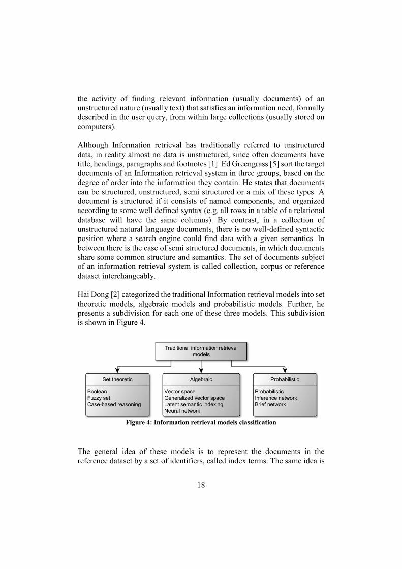
Hai Dong [2] categorized the traditional Information retrieval models into set
theoretic models, algebraic models and probabilistic models. Further, he
presents a subdivision for each one of these three models. This subdivision
is shown in Figure 4.
The general idea of these models is to represent the documents in the
reference dataset by a set of identifiers, called index terms. The same idea is
Figure 4: Information retrieval models classification
19
applied to the user query, which is represented by identifiers called search
terms. During the search (information retrieval phase), the index terms are
compared to the user query search terms, and those documents with more
terms in common with the user query, are said to be relevant to that query.
The index terms for each document are precomputed and stored in the index,
a data structure that organizes the index terms in such a way that it is easy to
perform the search later on. The set of index terms is called (index)
dictionary. Nothing is said about the nature of the documents, the user query
or the index/search terms. They could be text documents, images, audio files,
or any other type of information.
Set-theoretic models
Set-theoretic models represent documents as sets of words or phrases.
Similarities are usually derived from set-theoretic operations on those sets.
The Boolean model is based on Set theory and Boolean algebra. A set is a
collection of abstract objects, where each object is the member of this set.
Boolean algebra is a set of logical operations between two sets, such as
conjunction, disjunction and complement.
In the Boolean model, whether an index term appears in a document or not
determines the value of the weight between the index term and the document,
which is a binary value. A query normally consists of several index terms
connected by a set of logical operations, and it can be translated to a
conjunctive form which is composed of a number of conjunctive components
[8].
For example, we have a reference dataset with the documents shown in Table
2:
Doc id Document Index terms
1 “Central station, Lund” [central, station, lund]
2 “Gunnesbo station, Lund” [gunnesbo, station, lund]
3 “Central station, Malmö” [central, station, malmö]
Table 2: Document collection example and the associated index terms
A query like this: “central station” → (conjunctive form) → “central AND
station” will give the results shown in Table 3.

20
Doc id Match query?
1 Yes
2 No
3 Yes
Table 3: Example of document matching using Boolean model
Since documents 1 and 3 are the only ones that contain both terms, central and station.
If instead the query is “central station lund”, combining the terms with the
AND operator, we would only get document number 1, since it is the only
one that matches the query. Boolean model do not rank the results in any
way, just spot the documents that fulfills the requirements given in the query.
Algebraic models
Algebraic models represent documents and queries usually as vectors,
matrices, or tuples. The similarity of the query vector and document vector
is represented as a scalar value. These models let us rank the documents by
similarity. An example of algebraic model is the Vector space model [31,
32], in which each document is represented as a vector, and each dimension
of the vector corresponds to a term of the indexed terms as in Figure 5.
Figure 5: Vector space model example

21
If a term appears in a document, a weight is assigned to the corresponding
dimension in the vector. Similarly the user query can also be represented as
a vector with corresponding search terms. The relevance of a document given
a query can be calculated as the cosine of the angle between the two vectors
[8]. Depending on how the index terms are assigned, the documents in the
collection will be more or less similar to each other. Good index terms are
those that occur unevenly among the documents in the reference dataset. The
extreme case is an index term that appears only in one document, because a
query containing that term can only refer to one document. The reverse is
true for the bad index terms [33]. For instance, the word “the” is one of the
most commonly words found in English documents, therefore, the election
of “the” as vector dimension to represent documents, does not seem a good
choice to find individual documents among a collection. Figure 6 shows
graphically what happens after assigning an unevenly distributed index term.
After the assignment, the documents represented as vectors in the vector
space model are further from each other. Thus it is easier to identify them.
Using the document collection in Table 2, for the user query “central
station”, and assuming the algorithm assigns a constant weight of 1 to the
search and index terms, we would get these results shown in Table 4. In this
example, the dimensions of the vector space are {central, station, lund,
gunnesbo, malmö}. The query vector representation is (1,1,0,0,0). The
ranking is calculated using the cosine similarity between each document and
the query vector. Cosine similarity is explained later in section 2.2.2.
Figure 6: Vector space model, effect of assigning index terms

22
Doc id Doc. vector Ranking
1 (1,1,1,0,0)
2 (0,1,1,1,0) 0.577
3 (1,1,0,0,1) 0.816
Table 4: Example of document ranking using the Vector model and the cosine
similarity
The Extended Boolean model extends the Boolean model with the function
of term weighting, which is a hybrid model to combine the Boolean model
and the vector space model [19]. By weighting the association between a
document and a query term, the similarity between a conjunctive query, a
disjunctive query and a document can be calculated [9].
The query “central station”, would give the results shown in Table 5 for the
document collection in Table 2. The rankings are calculated using the cosine
similarity as in the previous example, but only for those documents which
fulfill the conditions imposed by the Boolean model. In this case the
document number 2 does not match the query, so it is discarded as a relevant
result for the query used in this example.
Doc id Match query? Ranking
1 Yes 0.816
2 No -
3 Yes 0.816
Table 5: Example of document ranking using the Extended Boolean model
Probabilistic model
Last, the fundamental of Probabilistic models is that they try to improve the
probabilistic description of the ideal answer set of documents relating to a
query by a series of iterations [8]. Given a user query and a document in a
collection, the probabilistic model tries to estimate the probability that the
user will find the interesting document. The model assumes that this
probability of relevance depends on the query and the document
representations only. Furthermore, the model assumes that there is a subset
of the documents which the user prefers as the answer set for the query. Such

23
an ideal answer set should maximize the overall probability of relevance to
the user. Documents in the ideal set are predicted to be relevant to the query,
and documents out of this set are predicted to be non-relevant [9].
2.2.1 Fundamentals of prefix and fuzzy search
The problem of devising algorithms and techniques for automatically word
prediction and correction in texts has been a main research challenge since
the early 1960s [21]. Traditional systems have used word frequency lists to
correct or complete words that the user has already started spelling out. Some
of the most extended techniques to predict and correct words are minimum
edit distance, n-grams and phonetic representations of words.
Minimum edit distance
By far the most studied spelling correction algorithms are those that compute
a minimum edit distance between a misspelled string and a dictionary entry.
The term minimum edit distance or Levenshtein distance was defined by
Vladimir Levenshtein [1965] as the minimum number of editing operations
(i.e., insertions, deletions, and substitutions) required to transform one string
into another [30].
Mathematically, the distance between two strings a and b is given by
where:
( )
( ) ( )
( )( )( ) ( )
.1
1
a,b
a,b
a,b
a,bai j
max i, j if min i, j = 0,
lev i 1, j +1lev i, j =
otherwisemin lev i, j +1
lev i 1, j +1b
ìï
ìï -ï ïí ï
-íïïï - -ïï ¹îî
( )jia b¹1 is the indicator function, which is equal to 0 when ai = bj and equal
to 1 otherwise.
In general, minimum edit distance algorithms require m comparisons
between the misspelled string and the dictionary, where m is the number of
the dictionary entries [21].

24
N-grams
Given a string s, i.e. a sequence of characters, and n-gram is any substring of
s of some fixed length n. A simple similarity measure between two strings is
to choose n and count the number of n-grams the two strings have in common
[22]. Given the strings “abc” and “bcd” with n=2, then the strings’ 2-grams
are:
String 2-grams
“abc” {“ab”, “bc”}
“bcd” {“bc”, “cd”}
A problem with this approach is that some information about the string is
lost. As we see in the example above, both strings have one 2-gram in
common, even though they are clearly not the same string.
A variation of the basic n-gram scheme allows efficient word prediction or
prefix search. The idea is to represent a word by its variable length n-grams,
always computed from the first character of the word. For instance, the word
“Sweden” can be represented by its variable length edge-gram set:
word Edge-grams
sweden [s, sw, swe, swed, swede, sweden]
Phonetic techniques
Phonetic models are a subtype of similarity key techniques. The notion
behind similarity key techniques is to map every string into a key such that
similarly spelled strings will have identical or similar keys. Thus, when a key
is computed for a misspelled string it will provide a pointer to all similarly
spelled words (candidates) in the lexicon [21]. Probably the best-known
phonetic algorithm is SOUNDEX [22], invented in 1918. SOUNDEX uses
codes based on the sound of each letter to translate a string into a canonical
form of at most four characters, preserving the first letter [22]. With time
some other models appeared that improve the phonetic accuracy of this
algorithm, such as METAPHONE and later DOUBLE METAPHONE,
which take into account other languages than English, and generates at most
two codes for each input, being the second an alternative code. There is more
information about how METAPHONE and DOUBLE METAPHONE work
in the original paper written by Lawrence Phillips [23].

25
2.2.2 Document Similarity and TF-IDF
In vector space model, documents and queries are represented as vectors,
where each component of the vector is the weight assigned to a term of the
document. The terms of the documents could be, depending on the type of
search the system is intended to support, phrases (ordered list of words),
single words (being a document represented by the words in that document),
or any other term resulting from the processing of the document words (for
instance, n-grams or metaphone code of a word) as described in the previous
section, 2.2.1.
“Term frequency–inverse document frequency” (tf–idf) is one of the most
commonly used term weighting schemes in today’s information retrieval
systems [20]. Tf-idf is a numerical statistic that is intended to reflect how
important a word is to a document in a collection or corpus.
The tf-idf weighting scheme assigns a weight to term t in document d given
by the product of term frequency in the document and the inverse document
frequency:
tdt,dt, idf tf = idf-tf ×
Tf provides a direct estimation of the occurrence probability of a term in the
document. The more occurrences of a term in a document the more relevant
that term is for the given document. Term frequency can be defined as:
, Number of ocurrences of term in document t dtf t d=
Or the normalized form:
,
Number of ocurrences of term in document
Total number of terms in document t d
t dtf
d=
Raw term frequency suffers from a critical problem: it does not take into
account the frequency of the term among the documents in the collection.
Terms that occur to often in the collection have very little or none
discriminating power.
Idf is a mechanism for attenuating the effect of terms that occur too often in
the collection. An immediate idea is to scale down the term weights of terms
with high collection frequency (cft), defined to be the total number of

26
occurrences of a term in the collection. The idea would be to reduce the tf
weight of a term by a factor that grows with its collection frequency. It is
more commonplace to use for this purpose the document frequency (dft),
defined to be the number of documents in the collection that contain a term.
Idf is usually defined as:
= logt
t
Nidf
df
æ öç ÷è ø
N is the size of the collection. Idft can be interpreted as ‘the amount of
information’ in conventional information theory, given as the log of the
inverse probability [20].
For example, imagine a document collection of N=10, in which every
document of the collection contains the word “the”. No matter what the term
frequency is, the idft will be zero, idft = log(1) = 0. Therefore, the weight
assigned to the vector component that represents the term “the” will be zero
for all the vectors representing the documents. Intuitively, since the term
“the” appears in all the documents in the collection, this term is not good for
searching criteria. Let’s say now that the term “geocoding” appears only in
one document once, the term frequency for “geocoding”, in that document
will be 1, while it will be 0 in the rest documents. The idft will be in this case
equal to log(10/1)=1. Tf-idf assigns a high weight to that term since
“geocoding” appears only in one document of the collection.
In other words, tf-idf assigns a weight w to the term t in document d that is:
1. higher when t occurs many times within a small number of
documents (thus lending high discriminating power to those
documents)
2. lower when the term occurs fewer times in a document, or occurs in
many documents (thus offering a less pronounced relevance signal)
3. lowest when the term occurs in virtually all documents.
Cosine similarity
Vector space model represents each document as a vector in which each
vector dimension corresponds to a term in the index dictionary, together with
a weight for each component that is given by the tf-idf value. For dictionary
terms that do not occur in a document, this weight is zero.

27
In the same way, queries can also be represented as vectors. The advantage
of this strategy is that, since both queries and documents are seen as vectors,
we can use some measure of similarity between vectors to score documents
given a user query. One possible solution is to use the cosine similarity of
their vector representations [1]. Given the query vector v(q) and a document
vector representation v(d), the cosine similarity is calculated as [31]:
( ) ( ) ( ) ( )( )| | ( )| |qvdv
qvdv=v(d)v(q),cosine=dq,similarity
rr
rr
××
2.2.3 Text indexing
The previous section introduced the paradigm of information retrieval, as
well as techniques for fuzzy and prefix search. The documents of the
collection and user query are represented by a set of identifiers, called
index/search terms. These terms can be anything from phrases, words, to n-
grams or metaphone codes. The way these terms are computed and stored
affects the search speed as well as the way the user can search for documents.
In order to make the search efficient, index terms are usually stored in data
structures called inverted indexes. An inverted index maps index terms to
documents, or document ids. That way, when a user wants to find the
documents relevant to a user query, the IR system does not need to read
through all the documents in the collection, it only needs to extract the
document id:s from the index whose documents contain the search terms of
the query.
If we use the document collection in Table 2, the inverted index for such a
collection would look like Table 6.
Index term Document ids Term freq Document freq
Central [1,3] [1: 1, 3: 1] 2
Station [1,2,3] [1: 1, 2:1, 3: 1] 3
Lund [1,2] [1: 1, 2: 1] 2
Gunnesbo [2] [2: 1] 1
Malmö [3] [3: 1] 1
Table 6: Inverted index for a document collection

28
Table 6 represents the inverted index, together with the term frequencies and
document frequencies of each term, used to assign weights to the document
terms as described in section 2.2.2.
This index strategy is efficient for searches such as “central station lund”.
However, a search like “centrl station” will return no results, since there is
no mechanism for correcting errors. The same applies for a prefix search like
“centr”, in this case the system would need to find index terms among the
dictionary following the pattern given by “centr*”, an expensive operation.
We could instead, create a reverse index in which the index terms are n-
grams of the document words, or metaphone codes to approximate the words
by their sound. In this case a match would be found if the metaphone codes
match or the number of n-grams in common is over a certain limit for
instance.
A more detailed description of text indexing, and inverted index tables can
be found in [1, 31, 32].
2.3 Evaluation metrics
The two elementary metrics to evaluate correctness in Information Retrieval
are [9, 18]:
Precision (positive predictive value): Percentage of retrieved documents that is relevant to the user.
Recall (sensitivity): Percentage of the documents relevant to the user query that are successfully retrieved.
relevant documents retrieved documentsrecall =
relevant documents
Ç
Besides these measures, geocoding systems can be evaluated taking into
account the geospatial properties of the documents. Common metrics for
evaluating the quality of geocoding results are completeness (or match rate),
positional accuracy, and repeatability [16]. In general, the geocoding quality
relevant documents retrieved documentsprecision =
retrieved documents
Ç

29
depends on several factors such as geographic areas of addresses, quality of
the reference databases, match scores, and geocoding algorithms [4].
The match rate is a statistical metric commonly used to measure the
geocoder’s ability to successfully determine a geocode for a given set of text
addresses. High match rates (above 90%) are possible, however there are
always street addresses that are difficult to geocode. Match rates typically
vary from 70% to over 90%. Match rates can be a good metric, but can be
misleading [14].
If we assume that for each query, the user expects to get one and only one
relevant result, being the result the geocode of the place the user is trying to
find, then the match rate can be defined as the average recall over a number
of n geocoding requests.
Match rate: Percentage of correctly geocoded places by the geocoding system.
Number of geocoded placesmatch rate =
Total geocoding requests
For systems with auto-complete features, keystroke saving can be a good
measure (percentage of keystrokes eliminated by integrating the prediction
method) [22]. However, keystroke saving highly depends on the format and
length of the addresses being tested.
Absolute keystroke saving: Difference between the original address length, and the query length when the address is found by the geocoder.
length lengthkeystroke saving = address - query
Relative keystroke saving (or keystroke saving percentage): Absolute keystroke saving divided by the original address length.
length length
length
address - queryrelative keystroke saving =
address

30
Last, it is important to know how much time it takes a system to perform an
action. In the case of a geocoder, that would be the time it takes to execute
the geocoding algorithm. This times does not take into account the round trip
time or the client side code intended to present the results of the geocoding
request, for example the JavaScript code.

31
CHAPTER 3
3 OpenStreetMap and Nominatim
This chapter describes the geospatial reference dataset used in the project,
OpenStreetMap, and the open source geocoder in which this project is based,
Nominatim.
3.1 OpenStreetMap
OpenStreetMap [6] is an editable map of the world, released with an open
content license, and created by volunteers. Everyone is free to contribute by
adding new geographical data to the map, and it is the origin of many projects
in different fields, such as geocoding, semantic analysis, map browsers and
map renderers, map editing tools.
The map data and map images are free to use for everyone, released with
OpenStreetMap license, and supported by the OpenStreetMap foundation,
which is an organization that performs fund raising in order to provide
servers to host the OpenStreetMap project, but it does not control the project
or own the data. It is dedicated to encouraging the growth, development and
distribution of free geospatial data and to providing geospatial data for
anybody to use and share [6].
3.1.1 OSM data model
The OSM data model consists of three different element types or data
primitives, plus a type to store metadata about the three data primitives:
· Nodes: points with a geographic position, they represent features
without a size.
· Ways: ordered list of nodes representing polylines or polygons if
closed. Used to represent features with linear shapes like rivers, and
areas like forests, parks, Etc.
· Relations: they are an ordered list of nodes, ways and other relations,
they represent relations between the elements they contain.

32
· Tags: they are key/value pairs used to store metadata about the map
features like names, type, physical properties. Tags are not free-
standing, but attached to one of the previous features.
OSM data elements represent physical features on the ground (e.g., roads or
buildings) using tags attached to its basic data structures (nodes, ways, and
relations). Each tag describes a geographic attribute of the feature being
shown by that specific node, way or relation.
OpenStreetMap's free tagging system allows the map to include an unlimited
number of attributes describing each feature. The community agrees on
certain key and value combinations for the most commonly used tags, which
act as informal standards. However, users can create new tags to improve the
style of the map or to support analyses that rely on previously unmapped
attributes of the features.
Most features can be described using only a small number of tags, such as a
path with a classification tag such as highway=footway, and perhaps also a
name using name=[name identifying the path]. But, since this is a
worldwide, inclusive map, there can be many different feature types in
OpenStreetMap [34].
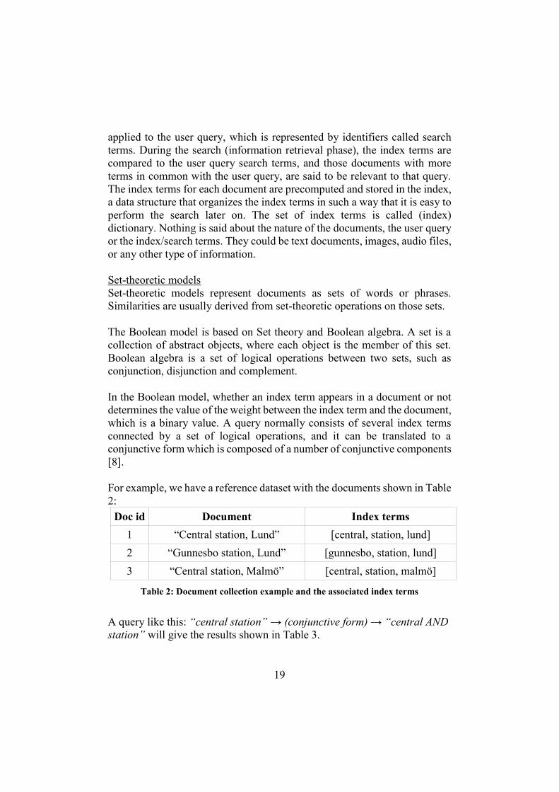
OpenStreetMap data is usually distributed in XML format, and each feature
is described with an XML element (<node>, <way> and <relation>) [7]. Text
1 is a small portion of the OSM data file for Sweden. The relation in this code
snippet corresponds to the definition of the Electronic building (E-huset), in Lunds Tekniska Högskola:
33
Table 7 lists the common attributes in each OSM element.
name value description
id integer
Used for identifying the element. Element types have
their own ID space, so there could be a node with
id=100 and a way with id=100, which are unlikely to
be related or geographically near to each other.
user string The display name of the user who last modified the
object. A user can change their display name
uid integer The numeric user id of the user who last modified the
object. The user id number will remain constant.
<?xml version='1.0' encoding='UTF-8'?>
<osm version='0.6' upload='true' generator='JOSM'>
<bounds minlat='55.7101169' minlon='13.2088387'
maxlat='55.7119181' maxlon='13.2123256' />
…
<way id='89001056' timestamp='2010-12-11T08:29:00Z'
uid='31450' user='sanna' visible='true' version='1'
changeset='6619970'>
<nd ref='1032852252' />
…
</way>
<relation id='1315684' timestamp='2013-10-07T08:46:15Z'
uid='13957' user='Grillo' visible='true' version='5'
changeset='18225042'>
<member type='way' ref='89001056' role='inner' />
<member type='way' ref='89001057' role='outer' />
<member type='way' ref='89001059' role='inner' />
<member type='way' ref='89001058' role='inner' />
<tag k='addr:city' v='Lund' />
<tag k='addr:country' v='SE' />
<tag k='addr:housenumber' v='3' />
<tag k='addr:street' v='Ole Römers väg' />
<tag k='building' v='yes' />
<tag k='name' v='E-Huset' />
<tag k='operator' v='Lunds Tekniska Högskola' />
<tag k='type' v='multipolygon' />
</relation>
… </osm>
Text 1: Example of OSM data in XML format

34
timestamp
W3C Date
and Time
Formats
time of the last modification
visible "true"
"false"
whether the object is deleted or not in the database, if
visible="false" then the object should only be
returned by history calls.
version integer
The edit version of the object. Newly created objects
start at version 1 and the value is incremented by the
server when a client uploads a new version of the
object. The server will reject a new version of an
object if the version sent by the client does not match
the current version of the object in the database.
changeset integer The changeset in which the object was created or
updated.
Table 7: OSM element, common attributes
In addition, tags, and also a full editing history of every element is stored [6].
3.2 Nominatim
This project is based on an open source geocoding solution called
Nominatim. Nominatim is an online geocoder written in PHP and it uses
OSM data as reference dataset.
Nominatim stores the OSM elements into postgreSQL, a relational database,
with PostGIS extension, a library of geospatial tools and types. The tool to
read and import OSM data in XML format into the database is called
Osm2pgsql.There is very little or no documentation on the implementation
and algorithms Nominatim uses, all the information have to be obtained from
the source code.
We could have chosen to create our index from the raw OSM data instead of
relying on Nominatim to make a first data processing. These are the
advantages and disadvantages of using Nominatim index over raw OSM
data.
Disadvantages:
· Nominatim index process takes several days, using the hardware that
runs the Nominatim project. The index time is around 250 hours, plus
2 days of the initial import process [6].

35
· Nominatim import process is lossy, meaning that some features are
not imported into the database. For example, Nominatim drops
coastlines and manipulates the data in a way that routing relationships
are lost [6].
Advantages:
· Nominatim calculates the parents of a place.
· Nominatim provides a database with geospatial indexes.
· Nominatim calculates information like country code, street and
postcode of OSM postal addresses if the information is missing.
· Nominatim assigns an address rank to each place.
· Nominatim (optionally) calculates a search rank to each place at
index time, based on the number of entries in Wikipedia that refers to
that place. This can be used to sort suggestions.
· Nominatim classifies the map features by class and type based on the
set of tags that identifies a feature.
· Nominatim provides tools to maintain the database.
3.2.1 Usage and statistics
The most recent Nominatim usage statistics were presented in the annual
conference, “OpenStreetMap. State of the map” in September 2013, in
Birmingham [17]. By that time, the server was handling 100 requests per
second, where 10% of the requests were search queries and 90% reverse
queries.
They also provided some numbers on the state of the database (Table 8).
Address type Number of entries in the database
(x106)
House number 60
Streets 47
POIs 12
Administrative areas 5
Water bodies 1.5
Total 130
Table 8: Database entries by type
36
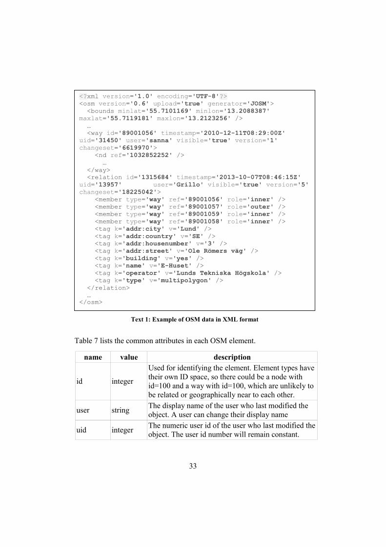
3.2.2 Database overview
This section is meant to be an overview of the main database relations
involved in the geocoding process in Nominatim. This chapter is not a
detailed view of the entire database structure. It focuses mainly on those
tables that contain the reverse index and/or are used to compute the address.
Figure 7 shows the tables used during the search process in Nominatim.
The dictionary of the inverted index is stored in the relation word (the term
word here is misleading, since what is stored in the word table can be actually
several words per entry. We will show an example later). During the import
process, for each new term to be indexed, a new entry is inserted. The word
column contains the original string, word_token contains the normalized
string, and search_name_count is the frequency of that word in the data set.
Each word gets assigned a word id word_id. The rest of the columns in this
table are used for filtering, like finding places by country code or Nominatim
class and type.
Search_name maps place id:s to word id:s. Nominatim classifies the index
terms for each place into two different lists, name_vector and
nameaddress_vector (the reason for this is to assign higher weight to the
tokens that are present in the name than the ones in the address). name_vector
Figure 7: Tables involved in the address search and computation process
37
contains the word id:s of the words that appear in the name of the place. In
the same way, nameaddress_vector contain the id:s of the words that appear
in the place parents. So, in the case of “E-Huset, Lund, Sweden”,
name_vector contains the word id corresponding to token “e huset” and
nameaddress_vector the word id:s of tokens “lund”, and “sweden”.
Placex stores the OSM elements, together with their tags, rank, parent id, and
class and type. It contains all the information needed to compute the address
string for a place given the place id and the preferred language. Placex.name contains a map of key/value pairs, each value being a different name or a
name in a different language. Keys for names in a specific language looks
like name:*, where the wildcard corresponds to a two-letter language code
defined in the standard ISO-639 [38]. So the translation of Göteborg in
English would be mapped in OSM and Nominatim like
name:en=>Gothemburg (if the translation exists). Nominatim also stores the
geometry and centroid of the element into this table. We will use this table
to compute the address of a place and retrieve the geometry and other
information as a response to a geocoding request.
During the import of new OSM data, Nominatim uses three intermediate
tables, osm_nodes, osm_ways and osm_relations. These tables contain raw
OSM nodes, ways and relations.
3.2.3 Processing OSM data
This section explains how Nominatim processes OSM data, which element
tags are processed, and how the index is built.
As explained before, OSM elements have associated tags with information
about the element, a subset of these tags contain information about the name
and address of the element. Nominatim processes the values of these tags to
compute the index terms associated to each OSM feature.
3.2.3.1 Processing feature names
For each OSM element, Nominatim processes the values of the tags in the
list as possible names for that element. It also processes the language variants
of the tags following the pattern [tag_name]:[language code in ISO 639-1].
For example, the OSM element corresponding to the city of Lund, Skåne län, Sweden, has an associated tag name=>Lund, and an additional tag name:ru=>Лунд which corresponds to the translation of Lund into Russian.

38
· name
· name:[lang]
· int_name
· common_name
· loc_name
· nat_name
· alt_name
· place_name
· official_name
· reg_name
· short_name
· old_name
· ref
· iata*
· icao*
· operator
*iata and icao are two especial tags to uniquely identify most major airports across the globe
Nominatim also processes the address tags associated with the element, i.e.
tags of the form addr:*. This is used to provide postal information for a
building or facility. Some possible tags are:
· housenumber
· housename
· street
· place
· postcode
· city
· province
· country
· ...
A complete list of these tags can be found in the OSM wiki [6] in the subsection map feature.
Before being indexed, each of the tags’ values listed above is normalized and
tokenized. The normalization process is as follows:
1. The tag value is lowercase
2. Diacritics are removed
3. The text is transliterated, text converted to Latin letters
4. Text words are transformed to common abbreviations
Once the tag value is normalized, Nominatim calculates the index terms by
which the element will be identified.
1. The normalized tag value is split using space character
2. The result of splitting the tag value is a list of tokens, some of these
tokens are too common to add any information to the index,
consequently are removed (for example the word “the” in English
texts)
3. The result is the index terms for that element
Figure 8 represents the different steps taken to process the tags.

39
3.2.3.2 OSM Administrative boundaries
Administrative boundaries [15] are subdivisions of areas, territories, or
jurisdictions recognized by governments or other organizations for
administrative purposes. Administrative boundaries range from large groups
of nation states right down to small administrative districts and suburbs.
OSM allows to specify the administrative level of the map features by adding
the tag boundary=administrative and admin_level = [1 to 10].
For example, the map feature representing the Swedish national borders is
assigned admin level 2. The Swedish administrative regions, like Skåne Län or Örebro Län, are assigned admin level 4. Last, the city areas, like
Stockholm or Malmö, are tagged as admin level 9. The admin levels are
used differently from country to country, the complete list can be found in
the OSM admin levels site [15].
Figure 8: Nominatim import: normalization and tokenization

40
3.2.3.3 OSM features hierarchy
All indexed features are converted to a simple hierarchy (rank) of importance
with points scored between 0 and 30 (where 0 is most important). Rank takes
account of differences in interpretation between different countries but is
generally calculated as:
Address type rank
Administrative boundaries: admin_level * 2 4–22
Continent, sea 2
Country 4
State 8
Region 10
County 12
City 16
Island, town, moor, waterways 17
Village, hamlet, municipality, district, borough,
airport, national park 18
Suburb, croft, subdivision, farm, locality, islet 20
Hall of residence, neighborhood, housing estate,
landuse (polygon only) 22
Airport, street, road 26
Paths, cycleways, service roads, etc. 27
House, building 28
Postcode 11–25 (depends on
country)
Other 30
Table 9: Address rank
For each feature down to level 26 (street level) a list of parents is calculated
using the following algorithm:
1. All polygon/multi-polygon areas which contain this feature (in order
of size).
2. All items by name listed in the is_in are searched for within the
current country (in no particular order).

41
3. The nearest feature for each higher rank, and all others within 1.5
times the distance to the nearest (in order of distance).
The tags of each parent of the element are also indexed and consequently,
used to find that element.
Buildings, houses and other lower than street level features (i.e., bus stops,
phone boxes, etc.) are indexed by relating them to their most appropriate
nearby street.
The street is calculated as:
1. The street member of an associatedStreet relation
2. If the node is part of a way:
2.1. If this way is street level, then that street
2.2. The street member of an associatedStreet relation that this way
is in
2.3. A street way with 50/100 meters and parallel with the way we
are in
2.4. A nearby street with the name given in addr:street of the feature
we are in or the feature we are part of
2.5. The nearest street (up to three miles)
2.6. Not linked
All address information is then obtained from the street. As a result addr:*
tags on low level features are not processed [24].
For interpolated ways simple numerical sequences are extrapolated (alpha
numerical sequences are not currently handled) and additional building
nodes are inserted into the way by duplicating the first (lowest) house number
in the sequence [6].
3.2.3.4 Index example
For each index term, i.e., a term which does not appear in the dictionary,
Nominatim creates a new entry into the word table. Table 10 shows a partial
view of the word table, with some of the indexed terms for “E-Huset, Lunds Tekniska Högskola, Lund, Sweden”.

42
word_id word_token search_name_count
2069 huset 206
17303 lunds 157
85819 tekniska 115
18403 hogskola 0
115540 lunds tekniska hogskola 0
312900 e huset 0
Table 10: Example of index terms in word table
The index terms in Nominatim are the normalized address words. These
index terms are later matched against the user query by Nominatim. The
consequences are:
· User can only search for full words, i.e., if a user query contains the
term lund, this will not be matched to the word id 17303, which
corresponds in the example to the term lunds. · The geocoder cannot correct any misspelling.
· There is no information about the language this index term
corresponds to, meaning that Nominatim does not split the index by
language, having to look up the whole index when trying to find a
match.
The same strategy is applied to the address tags of every OSM named
element, the tags addr:[housenumber/street/postcode/...] and so on. This
table forms the dictionary of the retrieval system, but it contains no reference
to the actual OSM places.
Nominatim maintains a map of index terms to place ids in search_name. Table 11 is a partial view of search_name for the entry mapping E-huset
building in LTH
place_id name_vector nameaddress_vector
1513474 [2069,312900] [17303, 85819, 18403, 115540,
place_id(Lund), place_id(Sweden)]
Table 11: Search name relation in Nominatim database

43
Finally, all the information about the element with id 1513474, E-Huset, can
be found in the relation placex, the geocoder uses this table to build the
localized address of that place. Table 12 is a partial view of the placex table
showing some of the information about the feature “E-Huset”.
place_id parent_place_id class type name ...
1513474 place_id(LTH) place house name=>'E-Huset',
name:en=>'Electronics
department'
...
Table 12: Placex relation in Nominatim database
3.2.4 Search algorithm
The search algorithm in Nominatim is written in PHP, and its extension is
around one thousand lines of code, plus some SQL functions. Nominatim
search algorithm finds matches between the user query search terms and
index terms obtained from the name and address tags of map elements and
its parents. The search algorithm can be described as follows.
1. The user query is normalized and split into tokens, commas help
finding address parts (This is the same process as the one described
in Figure 4)
2. Remove tokens, or token combinations that are not into the dictionary
(The dictionary is stored in the table word in the database).
3. Each valid token (or combination of tokens) is given a meaning,
either name, address or special term like OSM class, type, house
number, Etc.
4. A new search is executed for each token combination/meaning. i.e.,
guessing the token is part of the place name, or place address, or the
token is a house number etc.
5. After all searches are done, Nominatim has a collection of places,
these places are sorted by a) how many the terms from the search
query appear in the place name. Nominatim does not use any of the
mathematical models described in section 2.2, b) rank based on place
coordinates (if the user uses the web site, Nominatim assigns a
slightly higher relevance to the places located in the region of the map
the user is looking at) and c) importance assigned by Nominatim at
index time.
6. Addresses for each found place is computed, this includes address
translation to the requested language. See next section: Address
computation

44
7. Response is sent to the client.
3.2.5 Address computation
An address can be defined as a description of a real world place. Addresses
in Nominatim are not calculated and stored in the database beforehand, but
computed when a map feature is requested. Since each map feature has a
reference (parent_place_id) to its parent element, Nominatim simply
concatenates the place name of each parent in descending rank order.
Nominatim does not have any criteria to discern the representative parts of
an address, therefore, it often computes long address strings. The address
string returned by Nominatim for E-Huset in LTH is:
“E-Huset, 3, Ole Römers väg, Olshög, Tuna, Lund, Lund Municipality, Skåne län, Götaland, 224 64, Sweden”
The relevant parts of an address vary from country to country. In the example
above the address parts: Olshög, Tuna, Lund Municipality and Götaland can
be removed and the address text would identify the E-Huset map feature
uniquely.

45
CHAPTER 4
4 Proposed geocoder
This chapter proposes an extension to the Nominatim geocoder. The main
problem with the Nominatim geocoder is that, due to the indexing strategy,
there is very little flexibility in the way users can access the data. The
geocoder does not allow any spelling errors, neither get any feedback while
the user is typing the address. The reason for this is that addresses are
represented in the index by the address words, therefore, the search fails each
time one or more words are misspelled.
The proposed solution adds autocomplete and error correction functionality
to the Nominatim search module. It does not modify the way OSM map
features are imported into the Nominatim database, how these features are
later updated or how Nominatim classify them by class and type.
A naive approach would be for example to use the Levenshtein distance to
find addresses in the database similar to a user query, and rank the addresses
according to this distance. However, this approach is completely inefficient
since the Levenshtein distance needs to be calculated for each entry in the
database. We need a more scientific approach like the one described in
section 2.2.
In order to make autocomplete and error correction efficient, i.e. interactive
from the user perspective, a new index is designed. The proposed index
represents the addresses using n-grams and phonetic codes instead of words
(See section 2.2.1). This new approach of representing the addresses needs a
smarter way to evaluate the similarity with the user queries. The proposed
solution uses the Extended Boolean model for this purpose.
I build the proposed solution over a general-purpose search engine called
Elasticsearch [35]. As a general purpose search engine, Elasticsearch can be
setup to index documents in a variety of ways, for example using n-grams.
Also, Elasticsearch uses Extended Boolean model and Tf-idf to compute the
46
similarity between the user query and the indexed addresses. Elasticsearch
relies internally in Lucene [36]. Lucene is a general-purpose java library for
information retrieval which contains the implementation of the Extended
Boolean model, vector component weighting schemes like the Tf-idf
approach and functionality to calculate similarity between documents.
I used Elasticsearch to move from the original ad-hoc solution implemented
in Nominatim, to a more mathematical and scientific approach for indexing,
and searching addresses.
4.1 Elasticsearch Elasticsearch is an open source search engine first release in 2010. It is
available under the Apache 2 license, one of the most flexible open source
licenses [35]. The main features of Elasticsearch are:
· Full text search: Elasticsearch uses Java Lucene, a Java library for
Information retrieval. Lucene uses the Extended Boolean model to
build indexes and search for documents.
· Distributed: designed to grow horizontally as the size of reference
dataset grows. The index is distributed among several servers,
increasing the performance and robustness of the system.
· API driven: Elasticsearch is accessible from an API using JSON data
over HTTP protocol.
· Schema free: Elasticsearch allows to index JSON documents without
following any predefined schema. Later you can apply your domain
specific knowledge of your data to configure how the data is indexed.
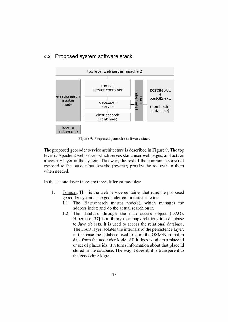
47
4.2 Proposed system software stack
The proposed geocoder service architecture is described in Figure 9. The top
level is Apache 2 web server which serves static user web pages, and acts as
a security layer in the system. This way, the rest of the components are not
exposed to the outside but Apache (reverse) proxies the requests to them
when needed.
In the second layer there are three different modules:
1. Tomcat: This is the web service container that runs the proposed
geocoder system. The geocoder communicates with:
1.1. The Elasticsearch master node(s), which manages the
address index and do the actual search on it.
1.2. The database through the data access object (DAO).
Hibernate [37] is a library that maps relations in a database
to Java objects. It is used to access the relational database.
The DAO layer isolates the internals of the persistence layer,
in this case the database used to store the OSM/Nominatim
data from the geocoder logic. All it does is, given a place id
or set of places ids, it returns information about that place id
stored in the database. The way it does it, it is transparent to
the geocoding logic.
Figure 9: Proposed geocoder software stack

48
2. Elasticsearch: Contains the index that gives support for fuzzy and
prefix search.
3. SQL database: PostgreSQL database with PostGIS extension. This
is the original Nominatim database, without any change.
The database contains the reference dataset, i.e. the map features
indexed by Nominatim. It is accessed to retrieve the geospatial
information of the requested address and compute the address
string.
4.3 Online geocoding service
The proposed solution is meant to work as an extension to the original
Nominatim geocoder. This means that the URL's pattern for the resources
and the request parameters and response formats are the same as in the
original Nominatim service. The URL’s structure is shown in Figure 10.
The web service offers 3 public resources: search, details and reverse, to
request a geocode operation (search), request a reverse geocode operation
(reverse), or get the details of an address. There is also a set of sub-resources
under the main resource “admin”. This set of sub-resources is useful for
indexing addresses, debugging and testing the system.
4.4 Address indexing
In order to support fuzzy and prefix search, Elasticsearch is setup to analyze
and compute more advance index terms than the ones used in the original
Nominatim geocoder.
Figure 10: Online service: URL pattern

49
During the index process, the proposed geocoder extracts one by one all the
Nominatim entries stored in the original database, and performs the next
operations on each one of them:
1. The geocoder calculates the index values of the index_name, i.e.
individual words from the name:* tags assigned to that OSM map
feature.
2. It computes and stores the Double metaphone values of these words
into values_dm.
3. It extracts the parents of the Nominatim entry from the database
(Nominatim offers a SQL function to obtain the parent id:s given a
place id). Each parent is assigned an address type depending on the
Nominatim class, type and admin_level OSM tag if it was assigned
to that entry. The possible address types that the proposed geocoder
uses are {housenumber, street, city, postcode, state, country, unknown}. If a parent matches an address type, its id is added to the
list of parent id:s used to build the address at search time. Otherwise
the address type is set to unknown. This is explained in more detail
in section 4.4.1.
4. The geocoder calculates the individual words of the names of the
parents that have been assigned an address type and their Double
metaphone codes.
5. Finally, the JAVA object containing the data calculated in the
previous steps is serialized in JSON format and sent to Elasticsearch.
The JSON object in Text 2 corresponds to the address “E-Huset, Lund Tekniska Högskola, Lund”.

50
Elasticsearch is setup to process each JSON field as explained in Table 13.
For instance, the address names are represented in the index by their n-grams
of minimum length 3, and also by the metaphone codes. The postal code field
is represented in the index by its edge-grams.
Document field Index strategy
place_id Unique id, the same as in Nominatim
database.
indexed_parent_ids Stored in Elasticsearch but not
indexed (they are not searchable).
{ "place_id":1513474, "osm_type":"R", "osm_id":1315684, "class":"place", "type":"house", "indexed_parent_ids":[515119,1513602,1517827], "importance":0.0, "address":{ "index_name":{ "short_terms":["E"], "values":[" E Huset Lunds Tekniska Högskola"], "values_dm":["LNTS","HST","KSKL","TKNS"] }, "index_road":{ "values":["Ole Römers väg"], "values_dm":["FK","RMRS","AL"] }, "index_city":{ "translation_map":{"ru":"Лунд"}, "values":["Lund"], "values_dm":["LNT"] }, "index_state":{ "translation_map":{"ru":"Сконе"}, "values":["Skåne Län”], "values_dm":["SKN", “LN”] }, "index_postcode":"22464", "index_country_code":"se" }, "centroid":[13.211050073039036,55.7110348], "calculated_address_type":"PLACE" }
Text 2: Example of serialized address into JSON

51
index_[name/road/city/state].values Analyzed using n-grams of minimum
size equals to 3. Any word shorter
that 3 chars is ignored.
index_[name/road/city/state].values_dm
This property contains the double
metaphone values of the tokens in
[name/road/city].values. The length
of these tokens varies between 2 and
4.
They are analyzed using edge-grams
(n-grams starting always from the
first character).
index_[name/road/city/state].short_terms
For short address tokens which will
be ignored (length <3 characters).
Indexed as it is.
index_postcode Analyzed using edge-grams.
index_country_code Not analyzed, indexed as it is, for
filtering by country code.
centroid Indexed as a geo-point type, for
spatial filtering.
Table 13: Document field index strategy
4.4.1 Address type computation
The address type of the Nominatim entries is computed using the class and
type attributes of the entry and the OSM administrative level if assigned
(admin_level attribute, see section 3.2.3.2). Table 14 shows the criteria to
assign the address type to a Nominatim entry.
Address type Condition(s)
House number class = place AND type = house
Street class = highway OR bridge OR tunnel
City class = place AND (type = city OR town OR village
OR hamlet) OR admin_level = city admin level
Postal code (class = place AND type = postcode) OR (class =
boundary AND type = postal_code)

52
State admin_level = state admin level
Country class = place AND type = country_code OR admin_level = country admin level
Unknown otherwise
Table 14: Criteria to assign the address type to the Nominatim entries
4.5 Searching addresses
The proposed geocoder relies on Elasticsearch to perform the search of
relevant addresses given a user query. Elasticsearch makes use of the
Boolean model to extract relevant documents given a user query. And then,
it ranks the relevant documents by representing documents and query as
vectors, and computes the similarity among the query and each document.
Elasticsearch provides a full query domain specific language (query DSL)
based on JSON to define queries. Elasticsearch queries specify what must be
searched and in which document fields must be found. However, the user
provides only a text query, and probably some extra information to apply
filters on the results. For this reason the user query needs to be processed and
translated to Elasticsearch queries.
4.5.1 Query processing
The query processor purpose is to assign some meaning to some parts of the
user query and to translate the user query into one or more Elasticsearch
queries (Figure 11). The input of the query processor is a formal query in text
format, expressing the user needs, for example if the user need is “to know
where the Electronics building in LTH is”, the associated query would be
something like “E-Huset, LTH, Lund”. The output of the processor is one or
more Elasticsearch queries, in which some of the words of each query might
have been given some meaning.
For instance, to find street intersections, the geocoder needs to find first the
streets to intersect. The query processor splits the user query in two
subqueries. The proposed geocoder split the queries at “?” character. Then,
the geocoder assigns a meaning to each subquery. In this case each subquery
is interpreted as the name of a street. The user query “Bytaregatan ? Knut
den stores gatan, Lund” will be interpreted by the proposed geocoder in the
following way: a request for finding the intersection of the streets
“Bytaregatan” and “Knut den stores gatan” in “Lund”.

53
The query processing is as follows:
1. The query is converted to lowercase.
2. Split the query in punctuation and space letter.
3. For each token which does not contain numeric characters, it
computes the double metaphone code.
4. Tokens whose length is 2 or lower are marked as short tokens.
5. Tokens containing numeric characters, these tokens might have a
special address meaning, like house number or postcode. These
tokens are analyzed as follows
5.1. If the query contains only one token, it is considered a postcode.
5.2. If the query contains more than one token, then tokens with
numeric characters have three possible interpretations, since they
can be part of the name, house number or postcode.
Last, after processing the query, the geocoder decides which type of search
it needs to perform. The search types are divided in four categories, basic
search, intersections, house numbers and addresses by postcode. The system
decides the search type following the next rules:
1. If the query contains the intersection character, the search type is set
to intersection, and then the geocoder search for addresses of type
street and derive the intersection geocode by finding the intersection
of the street line geometries.
2. If the query does not contain the intersection character, then the
system will behave as follows:
2.1. The geocoder search for addresses matching the words in the
user query.
2.2. If any of the search terms was marked as possible house number,
the system will try to find children of the addresses in the
previous step, matching such house number(s)
2.3. In the special case of having only one search term, that could be
a postcode, the geocoder find streets whose parent is the given
postcode.
Figure 11: Query processor input and output
54
4.5.2 Basic search
The diagram in Figure 12 shows the geocoding process, from the user query
to the final geocoded places response. First, the user query is processed and
translated into Elasticsearch queries. Second, the system searches into
Elasticsearch/Lucene index, and optionally apply filters, like spatial filter if
the user provided a search area. The output is a sorted list of place ids and
parent ids for each place. Last, the geocoder extracts the geocodes
corresponding to each place id and builds the address strings using the OSM
data stored in the Nominatim database.

55
Figure 12: Search algorithm

56
4.5.3 House number
House number search (Figure 13) is executed if any of the query terms was
identified as possible house number by the query processor. After the basic
search against Elasticsearch/Lucene index, if the system found any place of
type street, it will try to find children of those streets whose house number is
the one in the query.
This house number search is done against the Nominatim SQL database
using scanning, since as mentioned before, house numbers are not indexed
into Elasticsearch. After searching for streets, the system does not return
more than a few tens of places, so the scanning does not affect the response
time.
4.5.4 Street intersections
Street intersections are the only case of derived place returns. By derived we
mean that intersections are not precomputed at indexing time.
Street intersections are calculated in the following way (Figure 14). First, the
user query is divided into two subqueries, one per street. Next the geocoder
makes two independent searches against Elasticsearch, meaning that the
result of the first subquery will not affect the second search. On each search
Elasticsearch tries to find indexed places of type street by the name, and
maybe additional information like city, provided in the subquery. After this,
the geocoder has two lists of streets, or better, the place ids of these streets.
So next is to retrieve the geospatial information and name/address
Figure 13: House number search

57
information from the Nominatim SQL database. Once the geospatial
information is available, the system computes the intersections among the
streets in results #1 and results #2. Most of the intersection operations will
return an invalid intersection, meaning that there is no real intersection
between those street geometries, but some will return a point of intersection.
These are the relevant places the user is interested in. Next the geocoder
removes the invalid intersections and reevaluate the scores of the valid
intersections as the sum of the scores of intersected streets. Last it calculates
the address of each intersection as:
intersection address = [street 1 address] [intersection char ’?’] [street 2 address]
For example, if a user wants to find the corner of “Bytaregatan” with “Knut
den stores gatan” in “Lund”, the geocoder finds first streets by these names
located in “Lund” using Elasticsearch. Then it retrieves the geometries of
the found streets from the Nominatim database. Last it computes the
intersection of the geometries. If the intersection is not null, it’s a valid
intersection, and the final score is the sum of the individual scores assigned
by Elasticsearch for each street search. Otherwise it is removed from the
results.
Figure 14: Street intersections

58
4.5.5 Searching streets by postal code
This section introduces a new search type, addresses under a postcode. Postal
codes are used in some countries to divide geographical areas, stablish billing
strategies or as a way to narrow down the search of a postal address under a
postcode.
For example in the UK, taxi dispatchers usually search streets by typing first
the postcode they belong to. The goal of this search type is to find addresses
that are under a postcode. The original Nominatim geocoder returns instead
the centroid coordinates of the area a postcode refers to, being this
information of little value for the users.
Another example. The taxi business in UK, and especially in London,
charges their customers depending on their pickup and drop off postcode
addresses, which means that the postcode is the most used type of geocoding.
By presenting the user the addresses under that postcode, which in turn
correspond to a specific area of the city, we improve the user experience.
Due to the structure of the original Nominatim database, in which each of the
OSM map features indexed is assigned a parent id, the implementation of
this type of search is rather simple. Nominatim entries indexed in
Elasticsearch contains a postcode field, the geocoder just search for places
whose postcodes match or prefix match the (partial) postcode given in the
search query. The geocoder does not try to correct any possible mistake in
the postcode given by the user.
4.5.6 Building the addresses
The proposed geocoder follows the same strategy as Nominatim when
computing the address of a place. It calculates addresses by concatenating
the names of the place parents, but instead of taking one parent from each
address rank, and concatenate its name to the address, it concatenates the
names following a pattern defined for each country.
During the index process, the geocoder calculated a list of parent ids that is
now used to compute the address (see section 4.4). The geocoder uses this
list now to retrieve only the needed parents to build the address. This reduces
the amount of information the geocoder needs to extract from the database.
In addition, since a user will frequently search for places in a delimited
geographical region, the suggestions returned by the geocoder will have

59
common parents, reducing even more the information needed to compute the
addresses for all the suggestions. Imagine the query q gives as a result a set
of suggested places {s1, s2, s3}. Together with these suggestions,
Elasticsearch gives a list of parent id:s needed to compute the address of each
place (previously computed and stored), like the ones shown in Table 15.
Place id Parent id:s
s1 p1, p2, p3, p5
s2 p1, p2, p4, p5
s3 p2, p3, p5
Table 15: Example of parent id lists used to compute the place addresses
Next, the geocoder computes the union of parent id:s:
1 1 22 3 5 2 4 5 3 5 1 2 3 4 5p , p , p , p p , p , p , p p , p , p = p , p , p , p , pÈ È
These are all the Nominatim entries the geocoder needs to retrieve from the
Nominatim database in order to build the addresses for the response to the
query q.
We can define one address pattern for each country(i.e. the order in which
the different parts of the address are concatenated), since every Nominatim
entry has an associated country code with it, the geocoder will concatenate
the address parts following the pattern that matches the country code, or a
fallback if none is found. Table 16 shows the address pattern I defined for
Swedish addresses.
Country code Address pattern
fallback name, housenumber, street, city, postcode, country
SE name, housenumber, street, postcode, city, state, country
Table 16: Address pattern used for Sweden (SE)
Last the geocoder computes the addresses of each suggestion by
concatenating the names of the Nominatim entry and the parents, following

60
the pattern. Each address part is translated to the preferred language l indicated by the user, if a translation for that language exists.
address(r1, l) = name(p1, l), name(p2, l), name(p3, l)
The address computation process of the proposed geocoder is described in
the diagram in Figure 15.

61
This way of building the addresses is the answer offered to the research
question number 5 in section 1.2. I.e. how to improve the address
computation algorithm so the final address is shorter and contains only
relevant parent names.
We get two improvements compared to the original implementation in
Nominatim:
Figure 15: Address computation of a set of
places

62
1. The geocoder computes shorter addresses. The addresses contain
only the names of the parents whose address type appear in the
address pattern (patterns like the ones defined in Table 16).
2. The order of the address parts is defined in the pattern.
The motivation to assign an address pattern per country code is that address
formats usually differ from country to country. In some countries the house
number is written before the street name or vice versa. Also, in some
countries the state might be an important part of the address, while in others
it might be redundant information bloating the map feature.
Table 17 shows an example of the address calculated by the original
Nominatim geocoder and the proposed geocoder for the “E-huset” building
in LTH.
Geocoder Computed Address
Nominatim E-Huset, 3, Ole Römers väg, Norra universitetsområdet, Norr, Lund, Lund municipality, Skåne län, Götaland, 22464, Sverige
Proposed
geocoder
E-Huset, 3, Ole Römers väg, 22464, Lund, Skåne län, Sverige
Table 17: Example of computed addresses by the Nominatim and proposed geocoder
The address given by the Nominatim geocoder contains address parts that
provide little information to the user, like “Norra universitetsområdet, Norr, Lund, Lund municipality”, since the place can be identified uniquely even
without these address parts. On the contrary, the address computed by the
proposed solution is more clear and concise.
4.5.7 Scoring the addresses
Each address returned by the geocoder gets a score calculated in several
steps. First, Elasticsearch, using the concepts of Vector space model and
cosine similarity, calculates a score which is basically a function of the index
terms and query terms. The more query terms matching the index terms of
an address, the higher the score.
Then, the score is boosted by adding the importance which Nominatim
computes for each place at index time. This importance (a value between 0
and 1) is a function of:
1. Number of links in Wikipedia that relates to this place.

63
2. If no entry is found in Wikipedia about this place, a weighted value
of the inverse of the rank_address property of each map feature.
0.7540
rank addressimportance=
æ ö-ç ÷è ø
Finally the score is optionally boosted depending on the search type.
1. For intersections, the final score is calculated as the sum of the scores
of each street.
2. Since house numbers are not indexed in Elasticsearch, but the
geocoder performs a second lookup in the Nominatim database,
house number matches are not boosted in the original score. The
geocoder boosts the score of the found children matching the
requested house number.
( )final elasticsearch Nominatimscore = score +importance + optional boost
4.5.8 Filtering out addresses by relative score
The proposed geocoder filters out addresses whose score is lower than a
fraction of the highest score of the suggested addresses. In the proposed
geocoder I use 0.8 as threshold. I.e. given a list of suggested addresses, all
the addresses whose score is lower than 0.8 times the highest score are
removed from the suggestions.
For example, if we have a list of suggestions calculated by the proposed
geocoder in which the highest score is 100 and another result has been scored
with 10, since 10/100 = 0.1 < 0.8 that result is removed from the returned
suggestions.
The reason to impose this condition in the results list is that even if the user
query and an arbitrary address are “very different”, they might have an n-
gram (section 2.2.1) in common. Therefore Elasticsearch assigns a score
greater than zero, but that score might be too low compared to the highest
score found in the results offered by the proposed geocoder. As a
consequence, the precision (See section 2.3 for a definition of precision) of
the proposed geocoder increases, since it returns fewer results.

64
4.6 Proposed solution of a distributed geocoder service
The number of addresses indexed in Sweden is around 400K. If we were to
index the whole world, the number of Nominatim entries to index would
amount to several millions. For such a big collection, Elasticsearch allows to
split the index in different chunks also called shards. Each shard can be
maintained by one or more Elasticsearch nodes (for redundancy). This is a
convenient approach for a geocoder to offer global results, since each data
node needs to manage a small part of the index and the searches are computed
in parallel by the different data nodes. In the proposed solution, described
graphically in Figure 16, the top level Elasticsearch node works as a load
balancer, it knows the state of the master nodes and routes the query to the
less loaded. The master nodes coordinate the data nodes to perform a
distributed search, and aggregate the results returned by each data node.
Also, this solution offers reliability and a better performance, since the search
can be done in any of the shard replicas (Figure 16 shows an index with two
replicas, each replica assigned to a different node, for robustness)
Notes in the Figure 16:
1. Top level Elasticsearch node: This node acts as a "search load
balancer". It routes the search requests that arrive to the geocoder to
the less loaded master node.
Figure 16: Distributed geocoder, proposed solution

65
2. PostgreSQL database: It hosts the Nominatim data stored. The
geocoder accesses this database to index Nominatim places and to
compute the place addresses.
3. Elasticsearch master nodes: their task is to coordinate the distributed
search among the Elasticsearch data nodes and aggregate the results
return by each data node.
4. Elasticsearch data nodes: These are the nodes hosting the data. The
index is spread among 5 primary shards, hosted in one of the data
nodes. Each primary shard (in the picture represented as shards S1 to
S5) is copied into a replica hosted in a different data node
(represented as S1R1 and S1R2 for replicas 1 and 2 of shard S1 and
so on).
5. Index shards: They are small parts of the index maintained by the data
nodes. Each one of the 5 shards in which the index is divided is
replicated twice among the data nodes. If a data node is down, the
master node knows about it and it routes the search to another data
node hosting a replica.

66
CHAPTER 5
5 Test results
5.1 Evaluation methodology and tools
In order to evaluate the proposed geocoder, a set of tools and test resources
was implemented. These include a random address generator, a random text
error generator to simulate misspelled addresses, a set of tests written in Java
to evaluate the system and a web to adjust the test parameters and show the
test results.
5.1.1 Server specifications and configuration
The geocoding server was tested in a machine with the next specifications:
Processor Intel Core I7 – 2.2Ghz (x4 cores)
Memory 8GB RAM
Hard disk SSD 80 GB
Table 18: Server specifications
5.1.2 Random address generator
The addresses used to test the system are selected randomly among the
reference dataset, i.e. the OSM places stored in the Nominatim database. The
sub-resource .../admin/test/testFile/{size}/{lang} builds files containing lists
of size “size” of addresses which are used later as user queries to geocode.
The addresses can be translated optionally to the language defined by the
path parameter “lang”.
A file with 100 addresses was generated to test the system. The addresses
were computed without any translation, resulting in addresses written in
Swedish. Each Nominatim entry, identified by its Nominatim place_id,
contains the text address computed by the Nominatim geocoder and the
proposed geocoder (Text 3).

67
Since we aim to evaluate the fuzzy and prefix search in the proposed solution,
map features whose only name is of type reference (“ref:*” tags) in the
Nominatim database are not included in this file. The reason for this is that
references are in most cases a single letter or a letter and a number such as
“E 4”, the highway between Malmö and Stockholm.
5.1.3 Random text error generator
The goal of the error generator is to simulate a user which, while typing an
address, makes a mistake and misspells the address. The error generator takes
as input a text string. This is the address the user sends to the geocoder to
find the location of the address. The error generator alters the input address
by applying one of these operations on a single character: change, delete or
insert a character. The number of alterations can be defined in the test
settings. As a result, the output of the error generator is a modified text string
whose difference with the original text string can be measured using the edit
distance (See section 2.2.1).
For example, a user might be trying to geo locate “Bytaregatan 4c, Lund, Skåne län, Sweden”. The user expects to see suggestions in a dropdown box
offered by the geocoder while the user types in new characters. But it might
happen that he makes a mistake while typing in and he sends a query like
“Bytaregtan” to the geocoder. In this example, the user is missing an “a”
character. The mission of the error generator is to model the user errors.
5.1.4 Test setup
I designed the test algorithm in a way that it simulates the behavior of a user
that tries to find the location of an address. The behavior is modeled by these
rules:
1. The user knows more or less accurately how to spell the names of the
address.
... "518439" : { "elasticsearch" : "Hotel Scandic Triangeln, Föreningsgatan, 21145, Malmö, Skåne län, Sverige", "nominatim" : "Hotel Scandic Triangeln, Föreningsgatan, Rådmansvången, Norr, Malmö, Skåne län, Götaland, 21145, Sverige" }, ...
Text 3: Extract of the test addresses file

68
2. The user types in one character after another. Sometimes, either
because the user don’t know exactly the spelling of the address, or
because he or she makes a mistake typing the character, the user
introduces an error in the address text.
3. With each new character added to the user query, the geocoder
returns a list of places that prefix match the user query. The user
keeps typing characters until the desired address appears in the
suggestions of the geocoder response.
4. Once the desired address is among the suggestions, the user needs no
longer to keep typing new characters. The address is considered to be
found and the user has saved typing n characters, being n the
difference between the address text length and the user query length.
The test process simulates the user behavior described above. It tries to find
the addresses in the test address file. For each address in the file, the test
process adds characters at the end of query and requests the geocoder (either
Nominatim or the proposed geocoder) until the desired address appears in
the suggestions. When the geocoder returns the desired address, the test
process calculates various metrics for that search: precision, keystroke
saving, time spent, Etc. (the metrics definitions can be found in section
2.2.3). When all the addresses have been tested, the average values of the
metrics are computed. The described procedure is repeated 10 times for each
number of errors introduced. The resulting values are used later to compare
the geocoders.
The tests are setup using the parameters listed in Table 19:
Parameter Values
Geocoding service {Proposed geocoder, Nominatim geocoder}
Number of addresses 100
Number of errors in query [0, 4]
Number of addresses in the
response
{1, 5}
Number of executions 10
Table 19: Test parameters
The geocoder sorts the suggestions by similarity with the user query,
therefore the more similar addresses appear first in the suggestions list. The
more suggestions the geocoder can return per request (Number of addresses

69
in the response), the sooner the user will find the address among the
suggestions, and the less characters the user needs to type in. In the other
hand, if the geocoder returns too many suggestions it will be difficult for the
user to find the desired address among the suggestions, and the user will need
to keep typing to filter out suggestions.
5.1.5 Web test interface
Illustration 1 is a snapshot of the test user interface to evaluate the system. In
the left panel (panel number 1, Illustration 2) it is possible to select the file
containing the test addresses in JSON format, turn on and off different parts
of the search engine, such as phonetic search or n-grams search, and adjust
weights assigned to these searches. The central panel (panel number 2,
Illustration 3) shows the results after the tests are executed, percentage of
addresses found, average time the search engine spent per search, precision
and so on. Last, the right panel (panel number 3, Illustration 4) shows the
raw JSON response sent with the test results, this is useful in case someone
wants to see more detailed information like failed searches, query used for
such searches or the response time of a single search.
Illustration 1: Web test interface

70 Illustration 2: Detailed view of the panel number 1

71
Illustration 3: Detailed view of the panel number 2

72
Illustration 4: Detailed view of the panel number 3

73
5.2 Results
5.2.1 Proposed geocoder results
Table 20 shows the results of geocoding 100 addresses using the proposed
geocoder, with a maximum number of results returned set to 1. The number
of errors introduced in the prefix query varies from 0 to 4.
Table 21 shows the results of geocoding 100 addresses using the proposed
geocoder. In this case the maximum number of results returned is set to 5.
The number of errors introduced in the prefix query varies from 0 to 4.
5.2.2 Nominatim geocoder
Nominatim was only tested without errors in the user query since it does not
support fuzzy search. Prefix search is not supported either so Nominatim
returns addresses when there are no word prefixes in the query. Table 22
Table 21: Elasticsearch test results for max 5 addresses returned
max results: 5
# of errors 0 1 2 3 4
search time (ms) 20,90 19,94 16,94 15,24 15,07
match rate % 100,00 99,30 98,68 98,66 98,33
precision % 47,09 51,24 55,55 61,53 64,56
address length 49,60 49,63 49,76 49,76 49,87
query length 8,60 9,88 11,72 13,91 13,91
keystroke saving 41,00 39,75 38,04 35,85 35,96
keystroke saving % 82,66 80,09 76,45 72,05 72,11
max results: 1
# of errors 0 1 2 3 4
search time (ms) 23,37 18,54 15,85 13,87 14,33
match rate % 98,00 98,00 98,00 97,34 96,64
precision % 100,00 100,00 100,00 100,00 100,00
address length 49,66 49,66 49,66 49,88 50,00
query length 11,15 12,21 13,71 15,91 18,71
keystroke saving 38,51 37,45 35,95 33,97 31,29
keystroke saving % 77,55 75,41 72,39 68,10 62,58
Table 20: Elasticsearch test results for max 1 address returned

74
shows the results of the tests using the Nominatim geocoder, set to return 1
and 5 addresses per request.
5.2.3 Results discussion
Search time
The average search time is well below 100ms. The proposed geocoder, using
Elasticsearch as the core of the search engine, provides better search times
than the Nominatim geocoder, even though it implements a more advance
search algorithm.
The search time is lower the longer the user query. The reason for this is that
longer queries provide more information to the search engine (Elasticsearch)
about the address the user is looking up. Thus Elasticsearch is able to filter
out more results using the Boolean model, and needs to compute fewer scores
before passing the ids of the suggested addresses to the geocoder.
In a production server it would be more interesting to see the average round-
trip time, which includes the search time, network time and JavaScript time.
A maximum round-trip time around 300 ms lets the user experience an
interactive response [28].
Match rate
The test results in Nominatim gives as best 88% match rate (See section 2.3),
in the case of retrieving the top 5 addresses per request. If Nominatim only
retrieves the highest scored address, the match rate drops to 72%.
The results are much better in the proposed geocoder, in which the match
rate never falls below 96% even with 4 errors introduced in the user query.
Table 22: Nominatim test results for max 1 and 5 addresses returned
max results: 1 5
# of errors 0 1 0 1
search time (ms) 33,29 - 37,98 -
match rate % 72,00 - 88,00 -
precision % 100,00 - 60,00 -
address length 85,43 - 86,66 -
query length 13,98 - 12,00 -
keystroke saving 71,45 - 74,66 -
keystroke saving % 83,64 - 86,15 -

75
We observe that when the number of errors in the user query increases, the
user needs to type in more characters to find the address. I.e. the user needs
to provide more information about the address.
Precision
Due to the definition of precision (See section 2.3), this metric offers no
information for max addresses = 1, since the precision is measured when the
right address is found, and the geocoders do not suggest more than one
address. Consequently the precision is 100% when max addresses = 1.
Looking at the results when the number of suggested addresses is 5, and no
errors are introduced in the query, Nominatim (60%) has a slight advantage
over the proposed geocoder (47%). But the query needed to find the place
with Nominatim is longer than the query sent to the proposed geocoder. I.e.
the Nominatim geocoder needs more characters to find the right address
among the suggestions, these extra characters added to the query of course
increase the average precision.
Looking at Table 20 and Table 21, we observe that the proposed geocoder
needs more characters to find the right address the more errors are
introduced. The extra characters added to compensate the errors also helps
to identify better the address being looked up. Thus increasing the precision
of the suggestions.
Address length
The addresses computed by the proposed geocoder (49-50 characters) are in
average shorter than the Nominatim addresses (86-87 characters) since the
addresses calculated by the proposed solution only contain the parents
specified in the address pattern as described in section 4.5.6. On the contrary,
Nominatim builds the addresses by concatenating the names of all the parents
of a place. However, the proposed geocoder still offers better match rate with
shorter queries. The reason for this is that much of the information provided
in the Nominatim addresses is irrelevant to identify them. How to improve
the address computation algorithm was in fact one of the research questions
stated in section 1.2.
Relative keystroke saving
The relative keystroke saving (See section 2.3) in Nominatim is higher than
in the proposed geocoder. However as said in the section above (address
lengths), the addresses in Nominatim are longer, but much of the text in the

76
addresses is irrelevant. Consequently Nominatim queries need a lower
percentage of characters of the original Nominatim addresses to find the
relevant address.
In the proposed geocoder, the keystroke saving varies with the maximum
number of addresses returned. As expected, when the geocoder returns more
suggestions per request, the user needs to type fewer characters in the query
to find the desired address. If no errors are introduced and the maximum
number of addresses = 5, the proposed geocoder needs only 9 characters
(82.7% keystroke saving) to suggest the address the user is interested in,
whereas in the case of returning only 1 address the geocoder needs 12
(77.55% keystroke saving) characters in average to find that same address.
If the number of addresses returned is set to 5, the keystroke saving decreases
as the errors in the query increases. As explained before, the reason is that if
the user makes a mistake while typing the address, then the geocoder needs
more information (longer query) to find that address.
Extra resources needed
The new features added to the geocoder have an associated extra cost in terms
of resources needed. The size of the index to support fuzzy search and
autocomplete for the Swedish OSM addresses is around 100MB.
The original size of the PostgreSQL database used by Nominatim after
indexing and storing the Swedish OSM address dataset is around 1 GB, so
the new index increases the storing requirements by 10%. This estimation
matches the approximated overhead given in the Elasticsearch
documentation [35].
77
CHAPTER 6
6 Conclusions and future work
6.1 Conclusions
This thesis adds two must have features to the Nominatim geocoder that
many of the main online geocoders support already, fuzzy search and
autocomplete. The proposed geocoder is an extension to the Nominatim
geocoder, in which I based my work. The solution offered in this thesis
answers the research question of how to improve the search algorithm in the
Nominatim geocoder by applying mathematical models commonly used in
information retrieval systems. In practice, this is done by combining the
general purpose search engine called Elasticsearch with the Nominatim
geocoder.
Applying mathematical models to the reference dataset of the proposed
geocoder leads to a more flexible and interactive search algorithm than the
original search algorithm implementation in Nominatim. With the proposed
solution, the users get suggestions as they type searching for addresses. The
geocoder suggests the right addresses even if the user makes any misspelling
and/or typing error. During the tests, the proposed geocoder successfully
found the right addresses even with up to 4 errors in the query in a 98% of
the cases for the case of 5 addresses returned.
Besides the main contributions, fuzzy search and autocomplete, the proposed
geocoder also offers a solution to return more concise addresses than the ones
returned by the original Nominatim geocoder. Having tested one 100
addresses, the addresses computed by the proposed geocoder are a 42%
shorter than the ones provided by Nominatim (The proposed geocoder
average address length is 50 characters vs 87 characters average length of the
Nominatim addresses).
Also, the algorithm to build the address is more flexible than in the original
version, allowing to build the addresses based on patterns. These patterns can

78
be specified one for each country, depending on how the addresses are
usually written for each country.
6.2 Future work
There are many things that can improve the proposed geocoder system.
Some features that are still not implemented in the geocoder are search by
categories, i.e. searching addresses or places by the type of the place, for
instance “restaurants in Lund”, categories are not indexed yet into the
proposed geocoder. This could also help to index and search places without
a name, or possibly only a reference, as in many bus stops for instance, in
which the only information available besides the category is a 1 character
reference in many instances.
Also, the system needs to be tested against addresses in other languages. This
thesis only uses Swedish addresses as reference dataset. It would be
interesting to evaluate the geocoder with addresses written in an alphabet
different than Latin.
In the thesis, two new search types were added to the geocoder: addresses
under a postcode and street intersections. However, the proposed solution
does not allow many other types of addresses being used nowadays in some
countries. For instance, in Colombia, addresses can be given as relative to an
intersection, as in “50 meters from the intersection between [street 1 and
street 2]”.
The ranking algorithm can be improved to take into account the distance
from the user to the suggested addresses, or by boosting the relevance of the
suggested addresses that appear within the part of the map the user is
currently looking at.
Another possible future work could be the evaluation of the distributed
geocoder. In the simple case of this research, the number of documents was
small enough to index them all in the same node. Indexing the whole set of
map features in OSM is a much harder task. It can be solved by dividing the
index in different servers. This arises multiple questions such as, how is the
distributed index divided, and how does this affect the search performance?

79
References
[1] Manning, Christopher D., Prabhakar Raghavan, and Hinrich Schütze.
Introduction to information retrieval. Vol. 1. Cambridge: Cambridge
university press, 2008.
[2] Dong, Hai, Farookh Khadeer Hussain, and Elizabeth Chang. "A survey
in traditional information retrieval models." (2008).
[3] Goldberg, Daniel W. "Improving Geocoding Match Rates with
Spatially Varying Block Metrics." Transactions in GIS 15.6 (2011): 829-
850.
[4] Roongpiboonsopit, Duangduen, and Hassan A. Karimi. "Comparative
evaluation and analysis of online geocoding services." International Journal of Geographical Information Science 24.7 (2010): 1081-1100.
[5] Greengrass, Ed. "Information retrieval: A survey." (2000).
[6] OpenStreetMap wiki [Online]. http://wiki.openstreetmap.org/wiki
[7] Ramm, Frederik, Jochen Topf, and Steve Chilton. OpenStreetMap: using and enhancing the free map of the world. Cambridge: UIT
Cambridge, 2011.
[8] Ogawa, Yasushi, Tetsuya Morita, and Kiyohiko Kobayashi. "A fuzzy
document retrieval system using the keyword connection matrix and a
learning method."Fuzzy sets and systems 39.2 (1991): 163-179.
[9] Baeza-Yates, Ricardo, and Berthier Ribeiro-Neto. Modern information retrieval. Vol. 463. New York: ACM press, 1999.
[10] Janowicz, Krzysztof, Martin Raubal, and Werner Kuhn. "The
semantics of similarity in geographic information retrieval." Journal of Spatial Information Science 2 (2014): 29-57.
[11] Jones, Christopher B., and Ross S. Purves. Geographical information retrieval. Springer US, 2009.

80
[12] Robertson, Stephen, and Hugo Zaragoza. The probabilistic relevance framework: BM25 and beyond. Now Publishers Inc, 2009.
[13] Goldberg, Daniel W., John P. Wilson, and Craig A. Knoblock. "From
text to geographic coordinates: the current state of geocoding." Urisa Journal 19.1 (2007): 33-46.
[14] Hutchinson, Matthew, and B. Veenendall. "Towards using intelligence
to move from geocoding to geolocating." Proceedings of the 7th Annual URISA GIS in Addressing Conference. 2005.
[15] OSM Admin boundaries [Online].
http://wiki.openstreetmap.org/wiki/Key:admin_level#admin_level
[16] Zandbergen, Paul A. "A comparison of address point, parcel and street
geocoding techniques." Computers, Environment and Urban Systems 32.3
(2008): 214-232.
[17] Hoffmann, Sarah. “OpenStreetMap. State of the map, Nominatim
behind the scenes”. OSM annual conference. Microsoft PowerPoint file.
September 2013
[18] Saini, Balwinder, Vikram Singh, and Satish Kumar. "Information
Retrieval Models and Searching Methodologies: Survey." Information Retrieval 1.2 (2014).
[19] Salton, Gerard, Edward A. Fox, and Harry Wu. "Extended Boolean
information retrieval." Communications of the ACM 26.11 (1983): 1022-
1036.
[20] Aizawa, Akiko. "An information-theoretic perspective of tf–idf
measures."Information Processing & Management 39.1 (2003): 45-65.
[21] Kukich, Karen. "Techniques for automatically correcting words in
text." ACM Computing Surveys (CSUR) 24.4 (1992): 377-439.
[22] Zobel, Justin, and Philip Dart. "Phonetic string matching: Lessons
from information retrieval." Proceedings of the 19th annual international ACM SIGIR conference on Research and development in information retrieval. ACM, 1996.

81
[23] Philips, Lawrence. "The double metaphone search algorithm." C/C++ users journal 18.6 (2000): 38-43.
[24] Wikipedia: List of postal codes format by country [Online].
http://en.wikipedia.org/wiki/List_of_postal_codes
[25] OpenStreetMap wiki: address format [Online].
http://wiki.openstreetmap.org/wiki/Addresses
[26] Goldberg, Daniel W. "Advances in geocoding research and
practice."Transactions in GIS 15.6 (2011): 727-733.
[27] Jin, Liang, and Chen Li. "Selectivity estimation for fuzzy string
predicates in large data sets." Proceedings of the 31st international conference on Very large data bases. VLDB Endowment, 2005.
[28] Ji, Shengyue, et al. "Efficient interactive fuzzy keyword
search." Proceedings of the 18th international conference on World wide web. ACM, 2009.
[29] Nominatim geocoder wiki [Online].
http://wiki.openstreetmap.org/wiki/Nominatim
[30] Levenshtein, Vladimir I. "Binary codes capable of correcting
deletions, insertions and reversals." Soviet physics doklady. Vol. 10. 1966.
[31] Salton, Gerard, and Christopher Buckley. "Term-weighting approaches
in automatic text retrieval." Information processing & management 24.5
(1988): 513-523.
[32] Faloutsos, Christos, and Douglas W. Oard. "A survey of information
retrieval and filtering methods." (1998).
[33] Salton, Gerard, Anita Wong, and Chung-Shu Yang. "A vector space
model for automatic indexing." Communications of the ACM 18.11 (1975):
613-620.
[34] OpenStreetMap wiki: map features [Online].
http://wiki.openstreetmap.org/wiki/Map_Features

82
[35] Elasticsearch [Online]. http://www.elasticsearch.org/
[36] Apache Lucene [Online]. http://lucene.apache.org/
[37] Hibernate [Online]. http://hibernate.org/
[38] ISO 639 [Online].
http://www.iso.org/iso/home/standards/language_codes.htm

83
List of Figures Figure 1: Geocoding...................................................................................... 9
Figure 2: Goals ............................................................................................ 12
Figure 3: Geocoding process overview ....................................................... 14
Figure 4: Information retrieval models classification ................................. 18
Figure 5: Vector space model example ....................................................... 20
Figure 6: Vector space model, effect of assigning index terms .................. 21
Figure 7: Tables involved in the address search and computation process 36
Figure 8: Nominatim import: normalization and tokenization ................... 39
Figure 9: Proposed geocoder software stack............................................... 47
Figure 10: Online service: URL pattern ...................................................... 48
Figure 11: Query processor input and output.............................................. 53
Figure 12: Search algorithm ........................................................................ 55
Figure 13: House number search ................................................................ 56
Figure 14: Street intersections ..................................................................... 57
Figure 15: Address computation of a set of places ..................................... 61
Figure 16: Distributed geocoder, proposed solution ................................... 64
Figure 17: Distributed geocoder ................................................................. 64

84
List of Tables Table : Common causes and effects of errors of the geocoding process .... 17
Table : Document collection example and the associated index terms ....... 19
Table : Example of document matching using Boolean model .................. 20
Table : Example of document ranking using the Vector model and the
cosine similarity .......................................................................................... 22
Table : Example of document ranking using the Extended Boolean model22
Table : Inverted index for a document collection ....................................... 27
Table : OSM element, common attributes .................................................. 34
Table : Database entries by type ................................................................. 35
Table : Address rank ................................................................................... 40
Table : Example of index terms in word table ............................................ 42
Table : Search name relation in Nominatim database ................................. 42
Table : Placex relation in Nominatim database .......................................... 43
Table : Document field index strategy ........................................................ 51
Table : Criteria to assign the address type to the Nominatim entries ......... 52
Table : Example of parent id lists used to compute the place addresses .... 59
Table : Address pattern used for Sweden (SE) ........................................... 59
Table : Example of computed addresses by the Nominatim and proposed
geocoder ...................................................................................................... 62
Table : Server specifications ....................................................................... 66
Table : Test parameters ............................................................................... 68
Table 20: Elasticsearch test results for max 1 address returned ................. 73
Table 21: Elasticsearch test results for max 5 addresses returned .............. 73
Table 22: Nominatim test results for max 1 and 5 addresses returned ....... 74

85
List of Acronyms
API Application programming interface
BM Boolean model
DAO Data access object
Df Document frequency
DSL Domain specific language
ES Elasticsearch
GIR Geographical Information retrieval
GIS Geospatial information system
HTTP Hypertext transfer protocol
Idf Inverse document frequency
IR Information retrieval
ISO International Organization for Standardization
JSON JavaScript object notation
OSM OpenStreetMap
Tf Term frequency
URL Uniform resource locator
VSP Vector space model
XML Extended markup language

86
Appendix 1
A.1 Glossary
Boolean retrieval model
The Boolean retrieval model is a model for information retrieval in which we
can pose any query which is in the form of a Boolean expression of terms,
that is, in which terms are combined with the operators AND, OR, and NOT.
The model views each document as just a set of words [1]
Collection or Corpus
The group of documents over which we perform retrieval [1]
Dictionary/Vocabulary/Lexicon
The set of indexed terms [1]
Document
Any piece of information the information retrieval system is built over [1]
Document frequency
Measure related to a term which says the number of documents which
contain that term [1]
Geocoding
Geocoding is the process of converting postal address data into geographic
coordinates, i.e. latitude and longitude pairs [3] .The software performing the
geocoding process is called a geocoder, which can be divided into four
components: input, output, processing algorithm, and reference database [4]
Index
Data structure containing mapping of terms to documents, whose purpose is
to avoid linearly scanning documents for each retrieval operation [1]
Information need
Information need is the topic about which the user desires to know more [1]

87
Information retrieval
Information retrieval (IR) is finding material (usually documents) of an
unstructured nature (usually text) that satisfies an information need from
within large collections (usually stored on computers) [1]
Posting
An item in the posting list which records that a term appeared in a document
[1]. In the simplest case, a posting is a pair of the form (term, doc Id)
Precision
Precision is the fraction of retrieved documents that are relevant to a user
query
Online geocoding
An online geocoding service is a network-accessible component, sometimes
a module of a GIS, which automatically performs the geocoding process. It
is usually available on the Internet by utilizing a Web service interface. The
data entry, such as a place name, street address, or zip code, is passed over
the Internet using a communication protocol to the geocoding service [4]
Query
The information the user conveys to the computer in an attempt to
communicate with it [1]. It can also be defined as a formal statement of the
user information need.
Recall
Recall is the fraction of relevant documents that are retrieved [1]
Relevant document
A document is relevant if it is one that the user perceives as containing
information of value with respect to their personal information need [1]
Retrieval
It is the activity of finding and providing documents from within the
collection that are relevant to a user information need [1]
Term frequency
The number of times a term appeared in a document [1]

88
Term
The indexed units [1], if documents are of text nature, they can be
sentences, words, or any other char chain resulting from processing the
document (one possible document processing activity is tokenization).
Token
A token is an instance of a sequence of characters in some particular
document that are grouped together as a useful semantic unit for processing
[1]
Tokenization
Given a document (text document), tokenization is the task of splitting the
document into pieces, called tokens [1]
Vector space model
Information retrieval model in which documents and queries are
represented as vectors, and each dimension of the vector corresponds to a
term in the vocabulary [2]

Imp
rovin
g a
n o
pe
n so
urce g
eo
cod
ing
serve
r
Department of Electrical and Information Technology, Faculty of Engineering, LTH, Lund University, February 2015.
Improving an open source geocoding server
Víctor García
Series of Master’s thesesDepartment of Electrical and Information Technology
LU/LTH-EIT 2015-430
http://www.eit.lth.se
Vícto
r García
Master’s Thesis