improving the shuffled complex evolution scheme for ...news.cisc.gmu.edu/doc/publications/chu, w.,...

Improving the shuffled complex evolution scheme for optimizationof complex nonlinear hydrological systems: Applicationto the calibration of the Sacramento soil‐moistureaccounting model

Wei Chu,1 Xiaogang Gao,1 and Soroosh Sorooshian1

Received 19 February 2010; revised 4 May 2010; accepted 26 May 2010; published 25 September 2010.

[1] An innovative algorithm, shuffled complexes with principal components analysis(SP‐UCI), is developed to overcome a critical deficiency of the shuffled complexevolution scheme: population degeneration. Population degeneration means that, duringthe evolutionary search process, the population of search particles may degenerate into asubspace of the full parameter space, thereby missing the capacity of fully exploringthe parameter space. Being confined in a subspace may even lead the particle populationto converge to nonstationary points, which is a fatal malfunction. To overcome thisproblem, SP‐UCI employs the principal components analysis to detect the occurrence ofpopulation degeneration and remedy the adverse effects. The ensemble of calibrationsof the Sacramento soil moisture accounting model with the SP‐UCI method over the LeafRiver basin, Mississippi, retrieves the optimal parameter values with the lowest recordedroot‐mean‐squared error of simulated daily runoff against the observation. Moreover,the result also provides consistent (narrow ranges) model parameter distribution,which results in a better understanding of the model’s behavior, given the watershed’shydrologic features.

Citation: Chu, W., X. Gao, and S. Sorooshian (2010), Improving the shuffled complex evolution scheme for optimization ofcomplex nonlinear hydrological systems: Application to the calibration of the Sacramento soil‐moisture accounting model, WaterResour. Res., 46, W09530, doi:10.1029/2010WR009224.

1. Introduction

[2] The capability of hydrologic models in predictingrunoff has been improved through parameter calibration[Brazil, 1988; Sorooshian et al., 1993; Vrugt et al., 2006],which has motivated the development and improvement of anumber of automatic calibration methodologies over thepast several decades [Gupta and Sorooshian, 1985; Duanet al., 1992; Vrugt and Gupta, 2003]. Calibration is theprocess where the parameters of model components, forwhich direct observations are not available, are estimatedindirectly by minimizing the discrepancy between simulatedand observed model outputs. As previous results in hydro-logic literature have shown, calibration of conceptual rain-fall‐runoff (CRR) models has proven to be most challengingbecause of a variety of complexities associated with then‐dimensional parameter spaces of CRRmodels [Sorooshianand Gupta, 1983; Gupta and Sorooshian, 1983; Gan andBurges, 1990a, 1990b].[3] Calibration methods for hydrologic models mainly

fall into two categories: the direct search and the probabi-listic estimation of parameters. The direct search methodemploys simulations of biological evolutionary processes

[Goldberg and Holland, 1988; Eberhart and Kennedy, 1995;Storn and Price, 1997]. Typically, the procedure involvesselection of particles (samples) in the parameter spacethrough the use of competitive evolution schemes, such asthe simplex scheme [Nelder and Mead, 1965], swarmintelligence [Eberhart and Kennedy, 1995], and geneticmutation/selection [Goldberg and Holland, 1988], to repro-duce better offspring particles. After generations of evolu-tions, the population attempts to converge to a single locationin the search domain with the best set of parameter values.In hydrology, CRR models have been the focus of modelcalibration studies for decades. In 1992, a direct search skill,the shuffled complex evolution scheme developed at theUniversity of Arizona (SCE‐UA) [Duan et al., 1992], set amilestone in CRR model calibration. Numerous studiesusing various CRR models, including the Hydrologic Model(HYMOD), the Six‐Parameter (SIX‐PAR) model [Duanet al., 1992], and the National Weather Service RiverForecast System’s Sacramento soil moisture accounting(SAC‐SMA) model [Sorooshian et al., 1993; Duan et al.,1994] demonstrated that SCE‐UA is an effective, consis-tent, and efficient algorithm for global optimization ofmodel parameters.[4] In contrast with the direct search approach, probabi-

listic estimation treats model parameters as random variables.Techniques are developed to derive the joint probabilitydistribution of parameters conditioned on how well modelpredictions match provided observations. In the procedure,parameter estimation is not at a single point but with

1Department of Civil and Environmental Engineering, University ofCalifornia, Irvine, California, USA.

Copyright 2010 by the American Geophysical Union.0043‐1397/10/2010WR009224

WATER RESOURCES RESEARCH, VOL. 46, W09530, doi:10.1029/2010WR009224, 2010

W09530 1 of 12

http://dx.doi.org/10.1029/2010WR009224

probabilistic uncertainty descriptions over the parameterdomain. In favor of obtaining parameter uncertainty distri-bution, Beven and Binley [1992] and Beven and Freer[2001] used the generalized likelihood uncertainty estima-tion methodology, and Thiemann et al. [2001] applied theBayesian recursive method. However, the successes of thesemethods rely heavily on the correct estimation of likelihoodfunctions and a priori distributions. The posterior distribu-tion will converge correctly only if the estimations arecorrect; otherwise, it will fail.[5] The complicated nature of rainfall‐runoff processes

makes it difficult to model the subprocesses precisely andderive the adequate likelihood function or a priori distribu-tions for model calibrations. Therefore, in the above‐mentioned studies, the Gaussian distribution, its derivatives,and other simple standard distributions were arbitrarilyadapted as the likelihood function with uniform prior dis-tribution. These assumptions about the stochastic propertiesof model parameters have been viewed as, perhaps, toosimplistic to track the sophisticated response surfaces ofparameters of CRR models [Duan et al., 1992]. The studyby Thiemann et al. [2001], which includes comparisonsbetween probabilistic estimations and the SCE‐UA method,and this study indicate that, through a much slower proce-dure compared with the direct search approach, the results ofprobabilistic estimations usually converge to a region in theparameter space where the best points are different from thesolution of SCE‐UA, and these best points seldom achievedoptimal parameter values as good as those achieved bySCE‐UA.[6] Vrugt et al. [2003, 2006] developed a revised Markov

chainMonte Carlo (MCMC) approach named SCEM‐UA forhydrological model calibrations. In SCEM‐UA, the SCE‐UAprocedure is strictly followed, except that the Metropolisscheme replaces the simplex scheme as the search kernel.Assisted by the shuffled complex strategy, SCEM‐UA out-performs the traditional MCMC in CRR model calibration[Vrugt et al., 2003]. However, SCEM‐UA still uses Gaussian

(or other simple standard) distribution as the proposal dis-tribution, which jeopardizes its validity when applied tocomplex problems. Therefore, experiments in this studydemonstrate that SCE‐UA achieves much better parametersets than that achieved by SCEM‐UA.[7] As evident by its popularity [Thyer et al., 1999],

SCE‐UA has resulted in a successful and objective strategyto cope with difficult problems in global optimization, whichmakes it superior to other direct search and probabilisticestimation methods for hydrological model calibration. Thisstudy intends to strengthen and expand the robustness ofSCE‐UA by overcoming a critical deficiency that SCE‐UAexperiences in high‐dimensional or complex cases.[8] Our recent study in experimenting with high‐

dimensional problems revealed that the SCE‐UA methodsuffers from a critical problem: “population degeneration”.This is mainly due to overlooking a fundamental require-ment of direct search methods, which is that the searchingparticles should keep the capability of searching the fullparameter space through the entire search process. Popula-tion degeneration refers to the phenomenon that all search-ing particles are driven into a subspace (or hyperplane) ofthe original parameter space. As illustrated in Figure 1, ifthere are three parameters to be calibrated, the parameterspace is a three‐dimensional (3‐D) space. In this case,population degeneration means that all the particles fall on asingle plane, which is a subspace of the parameter space.Since the SCE‐UA uses linear operations (the Nelder‐Mead[1965] simplex method) on current particles to generate newparticles, the population will be confined on this plane in theremaining search. If the global optimum is not located onthis plane, the degenerated population will miss the globaloptimum and has the fate of misconvergence or even stag-nation at nonstationary points.[9] To overcome the adverse consequences of population

degeneration suffered by SCE‐UA, a new method, namedShuffled Complex strategy with Principal ComponentAnalysis (SP‐UCI), is developed. This new algorithm isformulated by integrating Principal Components Analysis(PCA) and some stage‐of‐the‐art techniques of evolutionarycomputation with SCE‐UA. As revealed in this study, PCAhas the potency of identifying lost dimensions and restoringsearches in the full parameter space. In another study (Chuet al., A new evolutionary search strategy for global opti-mization of high‐dimensional problems, submitted toInformation Sciences, 2010), we demonstrated that thismethod excels some prevailing direct search algorithms onoptimization of high‐dimensional or complex problems. Inthe current study, this method is applied to calibrate the SAC‐SMAmodel and study the parameter uncertainties. Results inthis study show that the proposed algorithm outperformsSCE‐UA in the following aspects: (1) It retrieves betterparameter values which further reduce the model simula-tion’s root‐mean‐squared error; (2) The SP‐UCI methodis more robust; (3) The ensemble of optimized parametersretrieved by SP‐UCI better delineates the uncertaintydistributions of model parameters. The latter helps themodeler and model users to better understand the modelbehavior.[10] This paper is organized as follows: In section 2, the

population degeneration phenomenon is discussed, and ourapproach to address it is articulated. Section 3 compares theresults of SCA‐SMA model calibration over the Leaf River

Figure 1. Illustration of population degeneration in athree‐parameter space. All sample particles fall onto a planedefined by the first two principal components (P1 and P2).

CHU ET AL.: IMPROVING THE SHUFFLED COMPLEX W09530W09530

2 of 12

basin using the SCE‐UA and the SP‐UCI algorithms. Veri-fication of the retrieved parameters by different methodsusing an independent data set is also presented. Sig-nificances and limitations of SP‐UCI are discussed insection 4. Finally, in section 5, we summarize and discussthe methodology.

2. Population Degeneration Phenomenon

[11] Before introducing the SCE‐UA algorithm anddiscussing its problem in high‐dimensional searches, weexemplify the task of model calibration as follows.[12] Given is a model,

f̂ t ¼ f xt; �ð Þ; ð1Þ

where xt is the time series of input vector, � is the parametervector with d components (parameters), and f̂ t is the timeseries of simulated outputs.[13] The task is the estimate,

� ¼ Argmin y ¼ F ft; f̂ t� ��

; ð2Þ

where ft is the time series of observed outputs and F( ft, f̂ t) isthe objective function.[14] The SCE‐UA procedure searching for the optimal �

includes five steps:[15] 1. Start the kth generation of the population Pk

including M particles �i and their function evaluationvalues yl:

Pk ¼ �l; ylð Þf gMl¼1; �l 2 Rd ; yl 2 R

[16] For the initial population P0, randomly select Mparticles �i from the parameter space Rd.[17] 2. Order particles {�l} according to evaluation values

such that y1 ≤ � � � ≤ yM (l = 1 is the best particle):

Pk ¼ �l; ylð Þf gMl¼1; y1 � � � � � yM

[18] 3. Distribute the ordered particles into p complexesCi, each contains m‐ordered particles (note that M = m × p).[19] 4. For each complexCi, i = 1, …, p,[20] 4.1. Randomly select (d + 1) particles to form a

simplex (as vertices).[21] 4.2. Evolve the simplex for k1 (a user‐defined

number) times to get offspring particles replacing the worstparticles.[22] 4.3. Break the simplex and return (updated) the

particles into the complex.[23] 4.4. Go to 4.1 and repeat for k2 (a user‐defined

number) times.[24] 5. Check whether the stop criteria is satisfied. If not,

break all of the complexes intoM individual particles and goto 1. If yes, Stop![25] The strength of the SCE‐UA stems from the syn-

thesis of concepts that have proven successful for globaloptimization. In the procedure, step 4 performs competitiveevolution using the multistart Nelder‐Mead [Nelder andMead, 1965] simplex scheme. By searching its vicinity, asimplex can find qualified offspring effectively but with the

risk of converging to a local minimum. In steps 2 and 3, thecomplex shuffling scheme is designed to rescue the multi-start simplexes from being trapped by local regions ofattraction (minima) and put them back on a course to searchfor the global minimum. As presented by Duan et al. [1992]and Thyer et al. [1999], the response surfaces of CRRmodels usually possess a number of complex features, suchas nonconvexity with numerous regions of attraction havingmultiple optima; discontinuous derivatives and roughnesson the response surface, where the roughness generatesnumerous minor local optima; and interaction betweenparameters, resulting in high correlations. In the SCE‐UA, acombination of the simplex and shuffled complex schemesmakes “systematic evolution of a complex of points span-ning the space, in the direction of global improvement”(Duan et al., 1992).[26] However, there is a fundamental requirement

underlying the SCE‐UA procedure: the particles in a pop-ulation (complex) should span the whole parameter space inorder to be able to explore the attractive region that leadstoward the global optimum. Here, “span the whole searchspace” means that the space spanned by the particle popu-lation should possess dimensionality equal to that of theparameter space. At an intuitive level, consider using asingle simplex for parameter calibration: it is well‐knownthat, for searching a two‐parameter space, the simplexshould have three vertices (particles) forming a triangle (noton the same line) so that the particles (vertices) span a two‐dimensional (2‐D) space (i.e., in any 2‐D coordinate systemformed by a basis, projections of the particles on each axishave a nonzero variance); for a three‐parameter space, thesimplex should have four vertices forming a tetrahedron (noton a plane) so that the particles span a 3‐D space (i.e., in any3‐D coordinate system formed by a basis, projections of theparticles on each axis have a nonzero variance), and so on.[27] This requirement is usually satisfiedwhen the SCE‐UA

with multiple complexes is applied to low‐dimensionalcases. However, for problems with high dimensionalities orfor circumstances when the model parameters possess highcorrelations (which is often the case for models that simulatereal‐world processes, such as the CRR models), thisassumption tends to be violated easily. When the violationoccurs (i.e., population degeneration), all of the particles of apopulation degenerate into a subspace of the originalparameter space. Geometrically, there exists at least onebasis in the space and, on one or more vectors of this basis,all of the particles are projected at the same point (zerovariance). These vectors are considered as lost dimensionsfor the population. In the SCE‐UA, because the offspringparticles are generated by linear combinations of their parentparticles, once population degeneration occurs, the newparticles will remain in the same subspace. Although theSCE‐UA involves a random resampling operation (in thesimplex scheme), it will not work until the linear operationfails and its efficacy decreases geometrically with dimen-sionality. Therefore, after population degeneration, the fateof the search will largely depend on whether the globaloptimum is still located inside the subspace. If the globaloptimum is excluded from the subspace, then a subsequentsearch will lead the population to converge to the “opti-mum” point within the subspace. This point could be a localoptimum or even a nonstationary point in the full parameterspace (i.e., a point with a nonzero gradient).


3 of 12

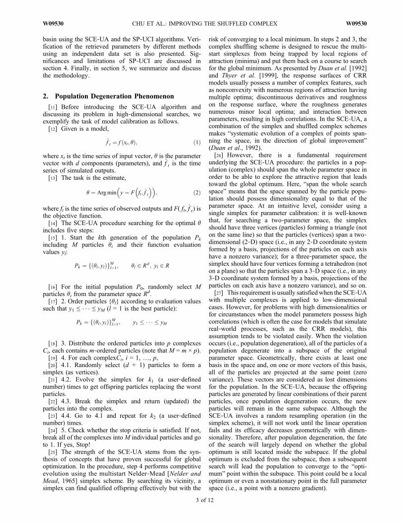
[28] We employed a composition benchmark functiondesigned by Liang et al. [2005] to demonstrate how easily thisnonfigurative phenomenon will occur in high‐dimensionalcases and the fatal consequences. This composition bench-mark function has been widely used to benchmark directsearch algorithms [Suganthan et al., 2005]. It allows the userto change dimensionality, the number of minima, the loca-tions of minima, and many other features of the responsesurface.

f xð Þ ¼X10i¼1

wi xð Þ fi0x� oið Þ=�ið Þ þ biasi

h i;with biasi ¼ i� 1ð Þ � 100 ;

ð3Þ

where x and oi are vectors in Rd, and d is the dimensionalityof the problem.

fi xð Þ ¼ jjxjj2

fi0xð Þ ¼ 2000fi xð Þ=jfmax ij; fmax i ¼ maxffi xð Þ; i ¼ 1; :::; 10g

wi xð Þ ¼ exp � fi x� oið Þ200�2

i

� �

! wi ¼wi if wi ¼ max wið Þwi 1�max wið Þ10� �

if wi 6¼ max wið Þ !(

wi ¼ wi=Xn¼10

j¼1

wj

[29] As shown in equation (3), this function is composedof 10 transformed sphere functions, fi′, with the minimumvalue of biasi located at oi. Therefore, f (x) has its globalminimum (= 0) at o1 and nine major local minima (= i ×100, i = 1, …, 9) at o2–10. Locations randomly generated inthe search space are o1–9, whereas o10 is set at the origin inorder to trap algorithms that take advantage of this speciallocation. To stretch (li > 1) or compress (li < 1) function fi′,li is used. The variable that controls the coverage range offi′ is si, a small si gives a narrow range. For CF1, s1–10 = 1and l1–10 = 0.05.

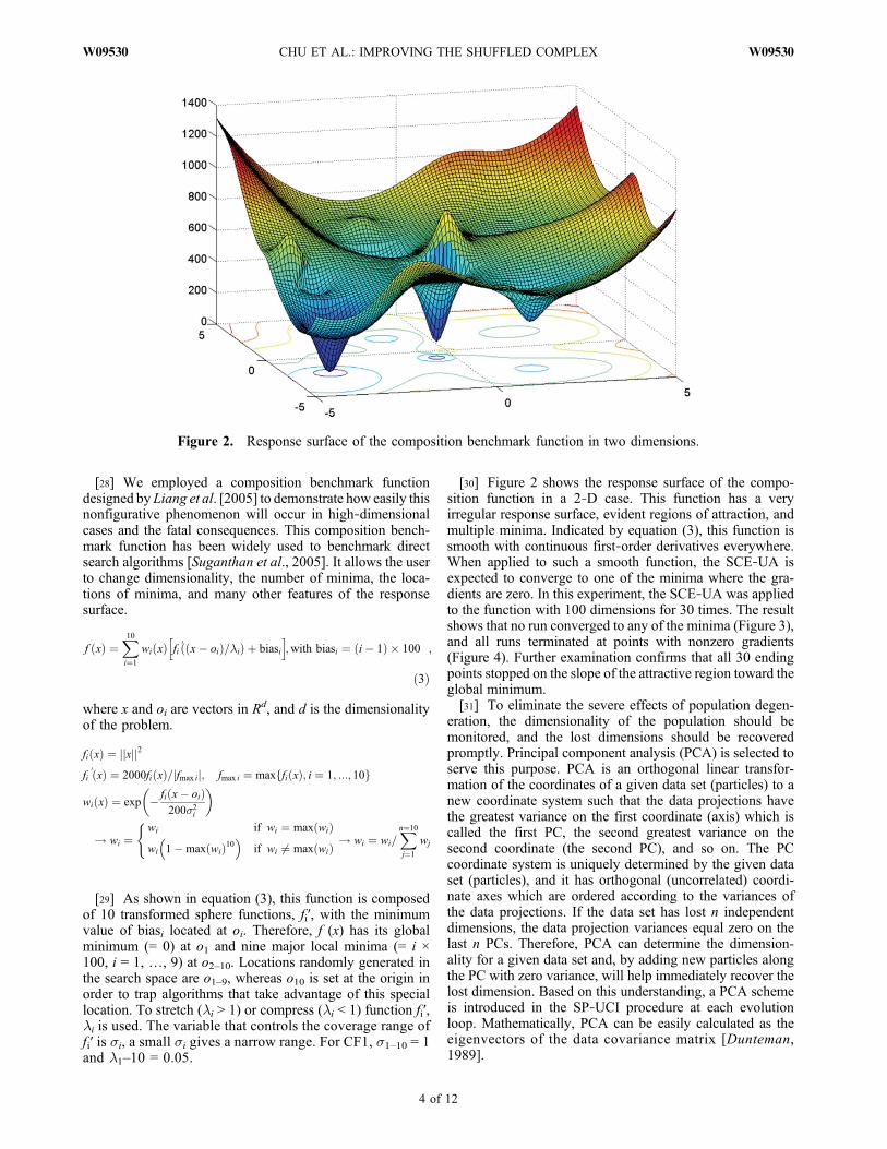
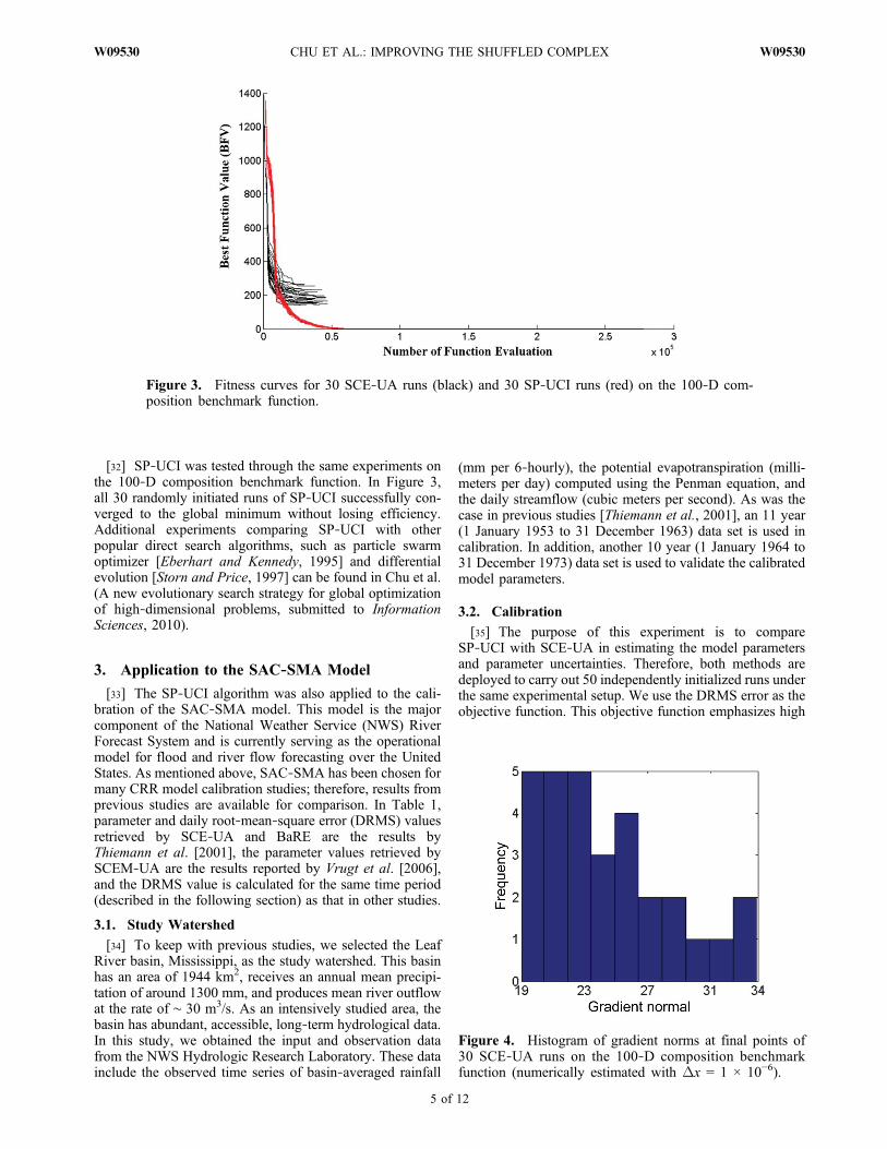
[30] Figure 2 shows the response surface of the compo-sition function in a 2‐D case. This function has a veryirregular response surface, evident regions of attraction, andmultiple minima. Indicated by equation (3), this function issmooth with continuous first‐order derivatives everywhere.When applied to such a smooth function, the SCE‐UA isexpected to converge to one of the minima where the gra-dients are zero. In this experiment, the SCE‐UA was appliedto the function with 100 dimensions for 30 times. The resultshows that no run converged to any of the minima (Figure 3),and all runs terminated at points with nonzero gradients(Figure 4). Further examination confirms that all 30 endingpoints stopped on the slope of the attractive region toward theglobal minimum.[31] To eliminate the severe effects of population degen-

eration, the dimensionality of the population should bemonitored, and the lost dimensions should be recoveredpromptly. Principal component analysis (PCA) is selected toserve this purpose. PCA is an orthogonal linear transfor-mation of the coordinates of a given data set (particles) to anew coordinate system such that the data projections havethe greatest variance on the first coordinate (axis) which iscalled the first PC, the second greatest variance on thesecond coordinate (the second PC), and so on. The PCcoordinate system is uniquely determined by the given dataset (particles), and it has orthogonal (uncorrelated) coordi-nate axes which are ordered according to the variances ofthe data projections. If the data set has lost n independentdimensions, the data projection variances equal zero on thelast n PCs. Therefore, PCA can determine the dimension-ality for a given data set and, by adding new particles alongthe PC with zero variance, will help immediately recover thelost dimension. Based on this understanding, a PCA schemeis introduced in the SP‐UCI procedure at each evolutionloop. Mathematically, PCA can be easily calculated as theeigenvectors of the data covariance matrix [Dunteman,1989].

Figure 2. Response surface of the composition benchmark function in two dimensions.


4 of 12

[32] SP‐UCI was tested through the same experiments onthe 100‐D composition benchmark function. In Figure 3,all 30 randomly initiated runs of SP‐UCI successfully con-verged to the global minimum without losing efficiency.Additional experiments comparing SP‐UCI with otherpopular direct search algorithms, such as particle swarmoptimizer [Eberhart and Kennedy, 1995] and differentialevolution [Storn and Price, 1997] can be found in Chu et al.(A new evolutionary search strategy for global optimizationof high‐dimensional problems, submitted to InformationSciences, 2010).

3. Application to the SAC‐SMA Model

[33] The SP‐UCI algorithm was also applied to the cali-bration of the SAC‐SMA model. This model is the majorcomponent of the National Weather Service (NWS) RiverForecast System and is currently serving as the operationalmodel for flood and river flow forecasting over the UnitedStates. As mentioned above, SAC‐SMA has been chosen formany CRR model calibration studies; therefore, results fromprevious studies are available for comparison. In Table 1,parameter and daily root‐mean‐square error (DRMS) valuesretrieved by SCE‐UA and BaRE are the results byThiemann et al. [2001], the parameter values retrieved bySCEM‐UA are the results reported by Vrugt et al. [2006],and the DRMS value is calculated for the same time period(described in the following section) as that in other studies.

3.1. Study Watershed

[34] To keep with previous studies, we selected the LeafRiver basin, Mississippi, as the study watershed. This basinhas an area of 1944 km2, receives an annual mean precipi-tation of around 1300 mm, and produces mean river outflowat the rate of ∼ 30 m3/s. As an intensively studied area, thebasin has abundant, accessible, long‐term hydrological data.In this study, we obtained the input and observation datafrom the NWS Hydrologic Research Laboratory. These datainclude the observed time series of basin‐averaged rainfall

(mm per 6‐hourly), the potential evapotranspiration (milli-meters per day) computed using the Penman equation, andthe daily streamflow (cubic meters per second). As was thecase in previous studies [Thiemann et al., 2001], an 11 year(1 January 1953 to 31 December 1963) data set is used incalibration. In addition, another 10 year (1 January 1964 to31 December 1973) data set is used to validate the calibratedmodel parameters.

3.2. Calibration

[35] The purpose of this experiment is to compareSP‐UCI with SCE‐UA in estimating the model parametersand parameter uncertainties. Therefore, both methods aredeployed to carry out 50 independently initialized runs underthe same experimental setup. We use the DRMS error as theobjective function. This objective function emphasizes high

Figure 3. Fitness curves for 30 SCE‐UA runs (black) and 30 SP‐UCI runs (red) on the 100‐D com-position benchmark function.

Figure 4. Histogram of gradient norms at final points of30 SCE‐UA runs on the 100‐D composition benchmarkfunction (numerically estimated with Dx = 1 × 10−6).


5 of 12

flows, which suits the mission of the SAC‐SMA model as apart of the NWS River and Flood Forecasting System. Manyother objective functions [Sorooshian et al., 1983] existwhich can provide more comprehensive measurements ofmodel performance. However, the purpose of this study is tocompare two methods, and a detailed study on selecting theobjective function is beyond the scope of this research.[36] As with previous studies, 13 parameters in the model

are calibrated, with the others set at default values. Theupper and lower bounds of the parameters are adopted fromBrazil [1988], as listed in Table 1.

3.3. Results and Discussion

[37] Performances of SP‐UCI and SCE‐UA in the50 individual runs are plotted in Figure 5. Similar to Figure 3,all of the SCE‐UA runs terminated earlier than SP‐UCI withworse DRMS values. In the SP‐UCI runs, the best DRMS is17.98 m3/s, which is better than the best one achieved bySCE‐UA (18.53 m3/s) and other previous studies, includingBrazil’s study [1988], BaRE [Thiemann et al., 2001], andSCEM‐UA (see Table 1). Since the SAC‐SMA model is nota smooth function, we cannot calculate the gradients at theending points to determine if the SCE‐UA runs stop at

Table 1. Comparison of Parameter Valuesa

UZTWM UZFWM UZK PCTIM ADIMP ZPERC REXP LZTWM LZFSM LZFPM LZSK LZPK PFREE DRMSb

Lower Bound 150.00 150.00 0.500 0.100 0.400 250.00 5.00 1000 1000 1000 0.250 0.025 0.600Upper Bound 1.00 1.00 0.100 0.000 0.000 1.00 1.00 1.00 1.00 1.0 0.010 0.00001 0.000Brazil 9.00 39.80 0.200 0.003 0.250 250.00 4.27 240 40 120 0.200 0.006 0.024 20.3SCE‐UA 14.09 63.83 0.100 0.000 0.363 249.97 2.46 238 3.19 99.8 0.019 0.021 0.001 19.2BaRE 33.61 76.12 0.332 0.016 0.266 117.30 4.95 236 132 124 0.089 0.015 0.146 21.8SCEM‐UA 10.70 32.55 0.39 5.1 × 10−4 0.10 241.46 1.66 261 16.96 45.08 0.19 0.01 0.10 21.6SP‐UCI 6.46 45.68 0.109 0.0001 0.363 241.08 1.80 260 11.9 80.1 0.25 0.017 0.0001 17.98

aUnit of all the capacity variables is mm and unit of DRMS is m3/s. Values estimated by Brazil [1988], shuffled complex evolution scheme developed atthe University of Arizona (SCE‐UA) and BaRE [Thiemann et al., 2001], and revised Markov chain Monte Carlo approach (SCEM‐UA) [Vrugt et al.,2006].

bDRMS stands for daily root‐mean‐square error.

Figure 5. Fitness curves for (top) 50 SCE‐UA runs and (bottom) 50 SP‐UCI runs for the calibra-tion of the SAC‐SMA model with historical data of the Leaf River basin. (DRMS denotes dailyroot‐mean‐square.)


6 of 12

nonstationary points. In Figure 6, the record of one SP‐UCIrun shows that, in six of the total 40 evolution loops, thePCA scheme identified and successfully remedied the lostdimensions. This observation is universal in all 50 SP‐UCIruns, and it indicates that, in the SCA‐SMA model cali-bration, population degeneration indeed occurs and can beremedied by the SP‐UCI method.

[38] In Figure 7, histograms of the final DRMS values for50 SCE‐UA runs and 50 SP‐UCI runs are plotted, respec-tively. In comparison to the SCE‐UA runs, the SP‐UCI runsconverge to smaller values of DRMS with a much reduceduncertainty range (SP‐UCI: 17.98–18.54 m3/s; SCE‐UA:18.53–23.67 m3/s). This improvement indicates that theSP‐UCI solution is more consistent and reliable.

Figure 6. The result of the principal component analysis scheme in a randomly selected SP‐UCI run. Ifthe start falls on the line of Yes, it means that, in the corresponding loop, population degeneration occurs,and the SP‐UCI procedure finds evident slope along one or more of the lost dimensions.

Figure 7. Histograms of daily root‐mean‐square (DRMS) values from the calibration runs of SCE‐UAand SP‐UCI, respectively. The solid line and the dashed line indicate the values of runs with parametersets of Brazil [1988] and SCEM‐UA, respectively.


7 of 12

[39] The consistency and superior performance of SP‐UCIare also witnessed when examining the hydrographs. In gen-eral, model simulations, generated with parameters obtainedfrom SP‐UCI, capture times and magnitudes of streamflowpeaks more accurately than those generated with parametersobtained from SCE‐UA. Figure 8 shows the simulated andobserved streamflows for the period of January–April, 1961.This time period contains the largest peak in streamflowthrough the entire 11 year period. From the plot, it can beclearly observed that the model with parameters retrievedbySP‐UCI simulates both peak flow and low flow betterthan the model with parameters retrieved by SCE‐UA.Model residuals of the same period are plotted in Figure 9.All model simulations underestimate the two largest peaksand overestimate the low flows. In keeping with the hydro-graphs in Figure 8, models calibrated by SP‐UCI have smallerresiduals compared with those calibrated by SCE‐UA.[40] Through the ensemble of randomly initiated direct

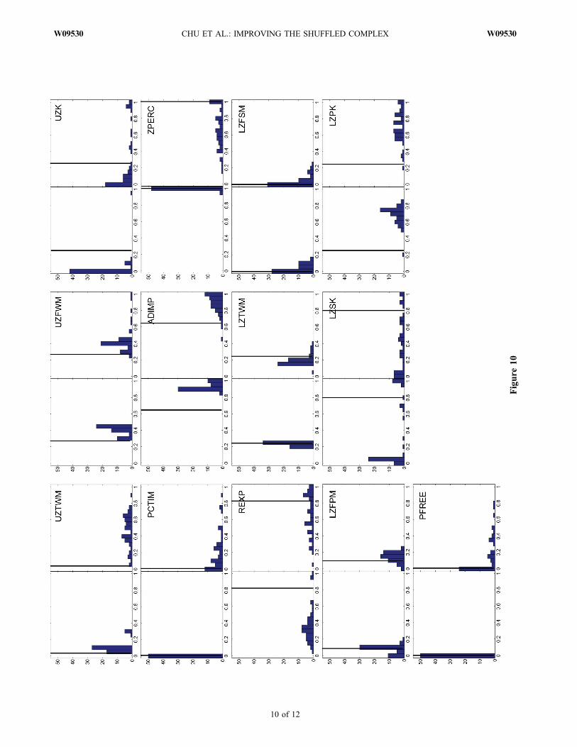
search using SCE‐UA and SP‐UCI, parameter uncertaintydistributions are also produced. In our experiments, 50 runswere conducted for each method. The distributions (histo-grams) of final parameter values obtained from both methodsfor 13 parameters are plotted in Figure 10. Clearly, SP‐UCIretrieves most parameters with smaller variances (uncertaintyranges) in comparison with SCE‐UA.[41] Parameter distributions produced from SP‐UCI can

shed light on model behavior given the hydrologic featuresof the basin. It is noticeable that the parameters labeledPCTIM (minimum impervious area) and PFREE (fraction ofpercolated water into lower zone free water) are both closeto their lower bounds, and the parameter labeled ZPERC(maximum percolation rate) is near its upper bound. Theseare in accordance with the results of Brazil [1988], whichwere obtained using a complicated multilevel calibrationstrategy based on long‐term observations in the watershed.Several inferences about the hydrologic properties of the

Leaf River basin can be drawn based on the SP‐UCIresults:[42] 1. The value of PCTIM close to zero means that the

watershed produces little immediate runoff in response torainfall.[43] 2. High ZPERC value indicates that a substantial

amount of water percolates into the lower zone, but thePFREE close to zero allows most of the percolated water toenter the lower zone tension water storage.[44] 3. Since most percolated water goes into tension

water storage, the functionalities of lower zone free waterstorages, both the primary and supplemental portions, areinsignificant. This fact is expressed by low storage capacities(LZFPM and LZFSM) and very insensitive lateral drainagerates (LZSK and LZPK), as shown in Figure 10.[45] Components of water balance in observation and

simulation over the simulation period are also examinedand compared. The ratios of annual runoff/precipitation,evapotranspiration (ET)/precipitation, and base flow/precip-itation are presented in Table 2. For the observation, ET iscalculated from water balance, ET = precipitation ‐ runoff,and base flow is calculated using the digital recursive filterwhich is formulated as [Chapman, 1991]

bk ¼ �bk�1 þ 0:5 1� �ð Þ fk þ fkþ1ð Þ;

where bk is the base flow, and the fast flow component fk canbe estimated from the total flow yk as

fk ¼ 3�� 1

3� �fk�1 þ 2

3� �yk � �yk�1ð Þ

[46] The filter coefficient a has the feasible rangebetween 0.9 ∼ 0.995.[47] The results show that, in average, simulations cali-

brated with SCE‐UA and SP‐UCI have similar partitions of

Figure 8. Hydrographs of the streamflow of the Leaf River basin over the period of January–April 1961(red points: observation; green lines: 50 simulations with the 50 parameter sets retrieved by SP‐UCI; bluelines: 50 simulations with the 50 parameter sets retrieved by SCE‐UA).


8 of 12

total runoff and ET and agree well with the observation.Difference in the baseflow components for the two groupsof simulations is evident. However, averages of both ofthem fall within the range of base flow calculated fromobservation with the feasible range of a.[48] It should be emphasized that the global optimization

method is superior to other popular stochastic frameworks inretrieving parameter uncertainties, such as Bayesian infer-ence and MCMC, because of the following two reasons:[49] 1. There is no assumption or simplification regarding

the studied parameter distributions, whereas many stochasticmethods are expected to work correctly only if the likeli-hood or proposal distribution can be correctly defined,which is extremely difficult. We want to clarify that, in thisstudy, the daily root‐mean‐square error is used only as astatistics measure to quantify the difference betweenobservation and simulation. We do not imply that the erroris following Gaussian distribution or that mean square erroris the maximum likelihood estimator.[50] 2. The distributions of model parameters are mean-

ingful only if the model performs well with the retrievedparameter values. Compared with the above‐mentionedstochastic methods, SP‐UCI prominently enhances the per-formance of the SAC‐SMA model over the studied basin[Thiemann et al., 2001; Vrugt et al., 2006].

3.4. Verification

[51] To test the validity of the parameter estimations fromcalibration, the verification experiment was also conducted.The data set of a 10 year period (1 January 1964 to31 December 1973) following the calibration period wasadopted to verify the calibration results. The parameter setsachieved by SCE‐UA and SP‐UCI, as well as those ofBrazil [1988] and SCEM‐UA (shown in Table 1), wereverified. The DRMS between model simulation and obser-vation of output flow is illustrated in Figure 11.[52] Similar to the results of calibration simulations,

parameter sets from the SP‐UCI calibration are superior tothose from the SCE‐UA in terms of lower DRMS mean andvariance. Furthermore, parameter sets from SP‐UCI con-sistently outperform those of Brazil [1988] and SCEM‐UA.

4. Discussion

[53] Employment of PCA is indispensable. PCA identifiespopulation degeneration and helps restore the population’scapability of searching the full parameter space, which is thefundamental requirement of any direct search method. ThePCA procedure requires additional computation time.However, for dimensionality lower than 1000, the compu-tation time of PCA is usually trivial compared to the com-

Figure 9. Model residuals (model output ‐ observation) of daily runoff of the Leaf River basin over theperiod of January–April, 1961 (top: 50 simulations with the 50 parameter sets retrieved by SP‐UCI; bot-tom: 50 simulations with the 50 parameter sets retrieved by SCE‐UA.

Figure 10. Distributions of 13 parameters that are calibrated in this study. For each parameter, the left graph shows thedistribution retrieved by the final results of the SP‐UCI method and the right graph shows the distribution retrieved by thefinal results of the SCE‐UA method. (Solid lines are estimation of Brazil [1988].)


9 of 12

Figure

10


10 of 12

putational time of model simulations. For instance, in theSAC‐SMA experiment, the PCA procedure takes only 0.1%of the computation time that required by running the modelsimulation one time[54] The SP‐UCI algorithm is a significant modification of

SCE‐UA, even for low‐dimensional problems. Intuitively,population degeneration is more prone to occur on high‐dimensional problems. However, in real applications, it ishard to tell beyond what number is considered highdimensional. For example, in the SAC‐SMA experiment,only 13 parameters were calibrated. But, because of thecomplexity of the model, population degeneration indeedoccurs and poses a difficulty for the SCE‐UA algorithm.Theoretically, population can occur on problems of any

dimensionality greater than two. Instead of running SCE‐UAwith the potential risk of population degeneration, oneshould consider SP‐UCI, which has a sound and solidpopulation‐monitoring and restoration scheme. As demon-strated in Figures 3 and 5, SP‐UCI shows similar efficiencywhen compared with SCE‐UA but with much better effec-tiveness and accuracy.[55] SP‐UCI has the same limitation as SCE‐UA, which is

that users need to adjust the algorithmic parameters, such asthe population size, number of complexes, and so on, tobalance the efficiency and effectiveness of the optimizationprocess [Duan et al., 1994]. Future work will be focused ondeveloping schemes for self‐adjusting algorithmic para-meters and designing specialized algorithms for individualpractical problems.

5. Summary and Conclusions

[56] Based on the SCE‐UA method, a new evolutionaryoptimization strategy, SP‐UCI, is developed to overcomethe population degeneration problem discovered in theapplication of SCE‐UA to high‐dimensional or complexproblems. Experiments on calibrating the SAC‐SMA modelwith 11 year historical data from the Leaf River basindemonstrate that SP‐UCI is more effective and more robustcompared with SCE‐UA. This is further substantiated by theresults of an independent verification on the data set of a

Figure 11. Histograms of daily root‐mean‐square (DRMS) values from the verification runs ofSCE‐UA and SP‐UCI, respectively. The solid line and the dashed line indicate the values of verificationruns of Brazil [1988] and SCEM‐UA, respectively.

Table 2. Components of Water Balances over the SimulationPerioda

Observation Mean SP‐UCI Mean SCE‐UA

Runoff/Precipitation 0.3330 0.3566 0.3562ET/Precipitation 0.6640 0.6428 0.6434Base flow/Precipitation 0.0870–0.1452b 0.1167 0.0990

aSP‐UCI denotes shuffled complexes with principal componentsanalysis, SCE‐UA denotes Shuffled Complex Evolution schemedeveloped at the University of Arizona, and ET denotes evapotranspiration.

bRange corresponding to the range of a of [0.900–0.995].


11 of 12

10 year period following the calibration period. SP‐UCIelevates the performance of the SAC‐SMA model in simu-lating the Leaf River basin to a very high level, achieved byno other method. Furthermore, the ensemble of SP‐UCIcalibrations can provide insight into model parameteruncertainty and, hence, can help in understanding the modelbehavior as expected from the historical hydrological data ofa particular catchment. The results from SP‐UCI are inaccordance with the more detailed study carried out byBrazil [1988], who used a multilevel calibration approach.[57] The discrepancy between model simulation and

observation may stem from several confounding sources,including input error, observation error, and model error.Furthermore, the model error can be considered as twocomponents: model structural inadequacy and modelparameter uncertainty. Global optimization methods explic-itly treat the model parameter uncertainty conditioned on theexistence of other errors. Improved optimization methodol-ogy results in a twofold benefit, as demonstrated by theexperimental results. First, from a user’s standpoint, betteroptimization methods can retrieve better parameter sets,which improve a model’s simulation and predictability.Second, from a modeler’s perspective, parameter sets esti-mated by good optimization methodology can better informthe developers whether or not the model is functioning asexpected and, if not, how to improve the model structure tobetter represent the underlying physical process.[58] This study demonstrates that SP‐UCI can improve

the SAC‐SMA model’s performance through parameteroptimization. However, the usability of this algorithmshould have a much wider range in many hydrologic inverseproblems.[59] The authors would like to provide the algorithm

codes upon email requests ([email protected]) in order tohave more application tests.

[60] Acknowledgments. The authors gratefully acknowledge thevaluable and constructive suggestions provided by the anonymousreviewers. The computation support was provided by Dan Braithwaite.Corrie Thies is also appreciated for her careful and professional editingof the manuscript. This research was supported by UCOP program ofUniversity of California (grant 09‐LR‐09‐116849‐SORS), CPPA programof NOAA (grants N080AR4310876 and NA050AR4310062) and NEWSprogram of NASA (grant NNX06AF93G).

ReferencesBeven, K. J., and A. M. Binley (1992), The future of distributed models:

Model calibration and predictive uncertainty, Hydrol. Processes, 6,279–298.

Beven, K. J., and J. Freer (2001), Equifinality, data assimilation, and uncer-tainty estimation in mechanistic modeling of complex environmentalsystems using the GLUE methodology, J. Hydrol., 249(1–4), 11–29.

Brazil, L. E. (1988), Multilevel calibration strategy for complex hydrologicsimulation models, Ph.D. dissertation, Colo. State Univ., Fort Collins,Colo.

Chapman, T. (1991), Comment on “Evaluation of Automated Techniques forBase Flow and Recession Analyses” by R. J. Nathan and T. A. McMahon,Water Resour. Res., 27(7), 1783–1784, doi:10.1029/91WR01007.

Duan, Q., S. Sorooshian, and V. K. Gupta (1992), Effective and efficientglobal optimization for conceptual rainfall‐runoff models, Water Resour.Res., 28(4), 1015–1031, doi:10.1029/91WR02985.

Duan, Q., S. Sorooshian, and V. K. Gupta (1994), Optimal use of theSCE‐UA global optimization method for calibrating watershed models,J. Hydrol., 158(3–4), 265–284.

Dunteman, G. H. (1989), Principal Components Analysis, 97 pp., SagePubl., Thousand Oaks, Calif.

Eberhart, R. C., and J. Kennedy (1995), A new optimizer using particleswarm theory, in Proceedings of the 6th International Symposium onMicro Machine and Human Science, pp. 39–43, IEEE Publ., Piscataway,N. J.

Gan, T. Y., and S. J. Burges (1990a), An assessment of a conceptualrainfall‐runoff model’s ability to represent the dynamics of small hypo-thetical catchments, 1. Models, model properties, and experimentaldesign, Water Resour. Res. , 26(7), 1595–1604, doi:10.1029/WR026i007p01595.

Gan, T. Y., and S. J. Burges (1990b), An assessment of a conceptualrainfall‐runoff model’s ability to represent the dynamics of small hypothet-ical catchments, 2. Hydrologic responses for normal and extreme rainfall,Water Resour. Res., 26(7), 1605–1619, doi:10.1029/WR026i007p01605.

Goldberg, D. E., and J. H. Holland (1988), Genetic algorithms and machinelearning, Machine Learning, 3(2–3), 95–99.

Gupta, V. K., and S. Sorooshian (1983), Uniqueness and observability of con-ceptual rainfall‐runoff model parameters: The percolation process exam-ined,Water Resour. Res., 19(1), 269–276, doi:10.1029/WR019i001p00269.

Gupta, V. K., and S. Sorooshian (1985), The automatic calibration of concep-tual catchment models using derivative‐based optimization algorithms,Water Resour. Res., 21(4), 473–486, doi:10.1029/WR021i004p00473.

Liang, J. J., P. N. Suganthan, and K. Deb (2005), Novel composition testfunctions for numerical global optimization, Proceedings of the IEEESwarm Intelligence Symposium, pp. 68–75, IEEE Publ., Piscataway,N. J.

Nelder, J. A., and R. Mead (1965), A simplex method for function minimi-zation, Comput. J., 7, 308–313.

Sorooshian, S., and V. K. Gupta (1983), Automatic calibration of concep-tual rainfall‐runoff models: The question of parameter observability anduniqueness, Water Resour. Res., 19(1), 251–259, doi:10.1029/WR019i001p00260.

Sorooshian, S., V. K. Gupta, and J. L. Fulton (1983), Evaluation of maxi-mum likelihood parameter estimation techniques for conceptual rainfall‐runoff models: Influence of calibration data variability and length onmodel credibility, Water Resour. Res., 19(1), 251–259, doi:10.1029/WR019i001p00251.

Sorooshian, S., Q. Duan, and V. K. Gupta (1993), Calibration of rainfall‐runoff models: application of global optimization to the Sacramento soilmoisture accounting model, Water Resour. Res., 29(4), 1185–1194,doi:10.1029/92WR02617.

Storn, R., and K. Price (1997), Differential evolution: A simple and effi-cient heuristic for global optimization over continuous spaces, J. GlobalOptim., 11(4), 341–359.

Suganthan, P. N., N. Hansen, J. J. Liang, K. Deb, Y. P. Chen, A. Auger,and S. Tiwari (2005), Problem Definitions and Evaluation Criteria for theCEC‐2005 Special Session on Real‐Parameter Optimization, pp. 1–50,Nanyang Technol. Univ., Singapore.

Thiemann, M., M. Trosset, H. Gupta, and S. Sorooshian (2001), Bayesianrecursive parameter estimation for hydrologic models, Water Resour.Res., 37(10), 2521–2535, doi:10.1029/2000WR900405.

Thyer, M., G. Kuczera, and B. C. Bates (1999), Probabilistic optimizationfor conceptual rainfall‐runoff models: a comparison of the shuffledcomplex evolution and simulated annealing algorithms, Water Resour.Res., 35(3), 767–773, doi:10.1029/1998WR900058.

Vrugt, J. A., H. V. Gupta, W. Bouten, and S. Sorooshian (2003), A shuffledcomplex evolution metropolis algorithm for optimization and uncertaintyassessment of hydrologic model parameters, Water Resour. Res., 39(8),1201, doi:10.1029/2002WR001642.

Vrugt, J. A., H. V. Gupta, S. C. Dekker, S. Sorooshian, T. Wagener, andW. Bouten (2006), Application of stochastic parameter optimization tothe Sacramento soil moisture accounting model, J. Hydrol., 325(1–4),288–307.

S. Chu, X. Gao, and S. Sorooshian, Department of Civil andEnvironmental Engineering, University of California, Irvine, CA 92697,USA. ([email protected])


12 of 12

improving the shuffled complex evolution scheme for ...news.cisc.gmu.edu/doc/publications/chu, w.,...

Documents