in situ observations of particle acceleration in shock ...blai/articles/11hietalaetal_jgr.pdfh....

In situ observations of particle acceleration in shock‐shockinteraction

H. Hietala,1 N. Agueda,2,3 K. Andréeová,1 R. Vainio,1 S. Nylund,4 E. K. J. Kilpua,1

and H. E. J. Koskinen1,5

Received 17 March 2011; revised 7 June 2011; accepted 12 July 2011; published 18 October 2011.

[1] We use detailed multispacecraft observations to study the interaction of aninterplanetary (IP) shock with the bow shock of the Earth on August 9–10, 1998. We candistinguish four different phases of particle acceleration in the shock‐shock interaction:(1) formation of magnetic contact with IP shock and the seed population of energeticparticles accelerated by it, (2) reacceleration of this population by the bow shock, (3) firstorder Fermi acceleration as the two shocks approach each other, and (4) particle accelerationand release as the shocks collide. Such a detailed analysis was made possible by theparticularly advantageous quasi‐radial interplanetary magnetic field configuration. To ourknowledge this is the first time the last phase of acceleration at a shock‐shock collision hasbeen reported using in situ space plasma observations.

Citation: Hietala, H., N. Agueda, K. Andréeová, R. Vainio, S. Nylund, E. K. J. Kilpua, and H. E. J. Koskinen (2011), In situobservations of particle acceleration in shock‐shock interaction, J. Geophys. Res., 116, A10105, doi:10.1029/2011JA016669.

1. Introduction

[2] Collisionless shock waves are an essential source ofenergetic particles in the heliosphere and beyond [Stone andTsurutani, 1985]. While most studies address the physics ofa single shock, shock‐shock interactions are also of impor-tance. Interplanetary (IP) shocks traveling in the solar windfrequently hit planetary bow shocks. Subsequent CoronalMass Ejections (CMEs) can interact in the inner heliospherewhile they travel toward the Earth [Lugaz et al., 2008]. Inthe outer heliosphere, shocks associated with Co‐rotatingInteraction Regions (CIRs) are observed to merge [Burlaga,1993]. Furthermore, Gómez‐Herrero et al. [2011] havereported observations of possible Interplanetary CME–CIRinteractions affecting the observed energetic ion fluxes at1 AU.[3] An early work on shock‐shock interaction and ener-

getic particles was the study by Scholer and Ipavich [1983].They compared the flux of 30–157 keV ions observed byISEE‐1 close to the bow shock of the Earth to the fluxobserved by ISEE‐3 far upstream, during the passage of anIP shock. During the shock crossing, ISEE‐1 detected apeak‐like enhancement of the flux, but this peak was notseen in the ISEE‐3 profiles. According to their interpreta-

tion, the peak was a result of particles upstream of the IPshock undergoing further acceleration at the bow shock.Reacceleration of energetic electrons in a similar setup withGeotail and Wind was briefly reported by Terasawa et al.[1997].[4] Later, particle acceleration in shock‐shock collisions

was investigated by Cargill [1991]. They used a one‐dimensional hybrid simulation with a quite small box size(for typical solar wind parameters it was a few Earth radii).Consequently the interaction time of the shocks was shortand the energy gain of the particles rather small. Morerecently, Lembège et al. [2010] have analyzed collisionsbetween quasi‐perpendicular non‐stationary shocks using a1D full particle‐in‐cell simulation.[5] In the laboratory, proton and deuteron acceleration has

been studied in the collision of two quasi‐perpendicularmagnetosonic shocks. Dudkin et al. [1992] [see also Dudkinet al., 1995] used a specific geometry where two low AlfvénMach number shocks collided at a fixed angle, with thebackground magnetic field lying between the two shockfronts. The energy of the accelerated ions streaming alongthe magnetic field reached 1–10 MeV.[6] In this paper, we present a detailed analysis of particle

acceleration in the interaction of an interplanetary shockwith the bow shock of the Earth. We first describe the mainfeatures of the multispacecraft data and the general char-acteristics of the IP shock in section 2. Section 3 discussesthe more detailed results of our analysis on the magneticfield structure and the energetic particle populations. Dis-cussion and conclusions are given in section 4.

2. Overview of the Event

[7] The data analyzed in this paper were obtained onAugust 9 and 10, 1998, by five spacecraft: ACE, Wind,

1Department of Physics, University of Helsinki, Helsinki, Finland.2Space Science Laboratory, University of California, Berkeley,

California, USA.3Departament d’Astronomia i Meteorologia, Institut de Ciències del

Cosmos, Universitat de Barcelona, Barcelona, Spain.4Applied Physics Laboratory, Johns Hopkins University, Laurel,

Maryland, USA.5Finnish Meteorological Institute, Helsinki, Finland.

Copyright 2011 by the American Geophysical Union.0148‐0227/11/2011JA016669

JOURNAL OF GEOPHYSICAL RESEARCH, VOL. 116, A10105, doi:10.1029/2011JA016669, 2011

A10105 1 of 12

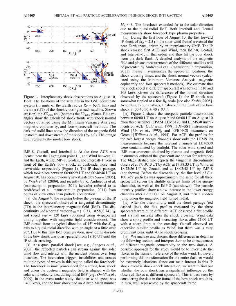
http://dx.doi.org/10.1029/2011JA016669

IMP‐8, Geotail, and Interball‐1. At the time ACE waslocated near the Lagrangian point L1, and Wind between L1and the Earth, while IMP‐8, Geotail, and Interball‐1 were infront of the Earth’s bow shock, at dusk‐side, nose, anddawn‐side, respectively (Figure 1). The IP shock passage,which took place between 00:06:29 UT and 00:48:48 UT onAugust 10, has been previously investigated by Szabo [2005],by Prech et al. [2009], and recently by K. Andréeová et al.(manuscript in preparation, 2011; hereafter referred to asAndréeová et al., manuscript in preparation, 2011) frompoints of view other than particle acceleration.[8] On August 9, the evening before the passage of the IP

shock, the spacecraft observed a tangential discontinuity(TD) in the interplanetary magnetic field (IMF). The dis-continuity had a normal vector nTD = (−0.33, −0.58, 0.74)GSEand speed vTD = 120 km/s (obtained using 4‐spacecrafttiming together with magnetic field considerations). TheIMF turned from its typical direction of 45° with the XGSE

axis to a quasi‐radial direction with an angle of a little over20°. Due to this new IMF configuration, most of the daysideof the bow shock was quasi‐parallel from 18:30 UT until theIP shock crossing.[9] At a quasi‐parallel shock [see, e.g., Burgess et al.,

2005], the reflected particles can stream against the solarwind flow and interact with the incident plasma over longdistances. The interaction triggers instabilities and createsmultiple types of waves in this region called the foreshock.The foreshock is most pronounced for a strong bow shockand when the upstream magnetic field is aligned with thesolar wind velocity, i.e., during radial IMF [e.g., Omidi et al.,2009]. In the event under study, the solar wind speed was∼400 km/s, and the bow shock had an Alfvén Mach number

MA ∼ 8. The foreshock extended far to the solar directiondue to the quasi‐radial IMF. Both Interball and Geotailmeasurements show foreshock type plasma properties.[10] During the first hour of August 10, the fast forward

IP shock of MA ∼ 2.5 (in the solar wind frame) traversed thenear‐Earth space, driven by an interplanetary CME. The IPshock crossed first ACE and Wind, then IMP‐8, Geotail,and Interball‐1, in that order, and thus hit the bow shockfrom the dusk flank. A detailed analysis of the magneticfield and plasma measurements of the different satellites willbe presented by Andréeová et al. (manuscript in preparation,2011). Figure 1 summarizes the spacecraft locations, theshock crossing times, and the shock normal vectors (calcu-lated using the Minimum Variance Analysis, magneticcoplanarity and four‐spacecraft methods). We estimate thatthe shock speed at different spacecraft was between 310 and365 km/s. Given the differences of the normal directionobserved by the spacecraft (Figure 1), the IP shock wassomewhat rippled at a few RE scale [see also Szabo, 2005].According to our analysis, IP shock hit the flank of the bowshock at 00:40:50 ± 40 s (UT).[11] Figure 2 shows the energetic particle observations

between 00:00 UT on August 9 and 06:00 UT on August 10from three satellites: EPAM‐LEMS120 and LEMS30 instru-ments on ACE [Gold et al., 1998], 3DP‐SST instrument onWind [Lin et al., 1995], and EPIC‐ICS instrument onGeotail [Williams et al., 1994]. For ACE, the profiles forthe two lowest energy channels show only the LEMS120measurements because the relevant channels at LEMS30were contaminated by sunlight. The solar wind speed andIMF measurements obtained by plasma and magnetic fieldinstruments onboard the spacecraft are shown for reference.The black dashed line depicts the tangential discontinuityobserved at 17:19:13UT byACE, at 17:58:33UT byWind, at18:23:56 UT by Geotail, and at 18:03:48 UT by IMP‐8(not shown). Before the discontinuity, the flux level of E >100 keV particles was approximately the same for all threespacecraft (given the slightly different limits of the energychannels), as well as for IMP‐8 (not shown). The particleintensity profiles show a slow increase in the lower energychannels after 12:00 UT on August 9, and then a suddenjump when the magnetic field turned radial.[12] After the discontinuity until the shock passage (red

dashed line), the flux profiles measured by the threespacecraft were quite different: ACE observed a flat profileand a small increase after the shock crossing. Wind datashow a spiky profile and increasing fluxes after 22:00 UTwith a sharp drop at the crossing. Geotail observed anotherwise similar profile as Wind, but there was a veryprominent peak right at the shock crossing.[13] We analyze and discuss these differences in detail in

the following section, and interpret them to be consequencesof different magnetic connectivity to the two shocks. Apossible approach for the study would be to investigate thefluxes in the frame of reference of the solar wind. However,performing this transformation for the entire data set wouldbe extremely laborious. Since our main interest in this IPshock event is shock‐shock interaction, we want to find outwhether the bow shock has a significant influence on theobserved fluxes at different spacecraft. This is best seen byconsidering the data in the frame of the bow shock which is,in turn, well represented by the spacecraft frame.

Figure 1. Interplanetary shock observations on August 10,1998: The locations of the satellites in the GSE coordinatesystem (in units of the Earth radius RE = 6371 km) andthe time (UT) of the shock crossing at each satellite. Shownare (top) the XZGSE and (bottom) the XYGSE planes. Blue tri-angles show the calculated shock fronts with shock normalvectors obtained using the Minimum Variance Analysis,magnetic coplanarity, and four‐spacecraft methods. Thedark red solid lines show the direction of the magnetic fieldupstream and downstream of the shock (BX < 0). The orangeline represents the model bow shock.

HIETALA ET AL.: PARTICLE ACCELERATION IN SHOCK-SHOCK INTERACTION A10105A10105

2 of 12

Figure

2.Observatio

nsof

theACE,W

ind,

andGeotailsatellites.From

topto

botto

m:om

nidirectionalintensities

ofener-

getic

particleflux

(ions)in

differentenergychannels,solar

windspeedu,

andthemagnitude

B,latitu

de�(−90°to

90°),and

longitu

de�(0°to

360°)of

theinterplanetary

magnetic

fieldin

GSE.The

ACEprofileswereobtained

bycombining

the

LEMS30

andLEMS12

0measurements

(assum

ingthat

thesystem

atic

errors

arelarger

than

thestatisticalon

es),except

forthetwolowestenergy

channels

forwhich

theLEMS30

measurements

show

clearsunlight

contam

ination.

The

black

dashed

lineshow

sthebeginningof

thequasi‐radialIM

F(tangentiald

iscontinuity);theredoneshow

stheIP

shockpassage.


3 of 12

[14] The probability that any of the energetic particlesstudied here were of magnetospheric origin is small. The Dstindex indicates that the magnetosphere was recovering froma storm induced by a previous CME passage. There was nosubstorm activity, indicated by the AE index ]100 nT.During the day following the IP shock passage (August 10),however, several substorms of AE ∼ 800 nT were triggered.Some of these were accompanied by energetic particlebursts in the few hundred‐keV range seen by Geotail andpartly by Wind as well (not shown).

3. Results

3.1. Magnetic Connection to the IP Shock and the SeedPopulation

[15] According to our analysis, the beginning of the quasi‐radial IMF on August 9 corresponds to the spacecraftmoving into a flux tube that is connected to the IP shockfront. Our analysis of the magnetic field is illustrated inFigure 3, where we have drawn the spacecraft magnetic fieldmeasurements as “frozen‐in” to the solar wind flow togetherwith the backwards propagated shock front measurements.We also traced sunwards the field line passing through thespacecraft location after the tangential discontinuity, byassuming that the magnetic field depends on the X coordi-nate only. For a quasi‐radial IMF configuration this is areasonable assumption for a period of observations with nodiscontinuities.[16] We find that in the XYGSE plane (Figure 3a), the

traced “frozen‐in” magnetic field line is quite straight, andmore radial than the nominal Parker spiral. Both linear(purple) and very long wavelength sinusoidal (green) fits areconsistent with the data. The ZGSE ‐component, on the other

hand, is well fitted with a sine wave of l ∼ 2200 RE (seeFigure 3b). This is of the same order as the observedmagnetic field correlation length of a few thousand Earthradii [Matthaeus et al., 1986]. We interpret this fluctuationas a large scale Alfvén wave: The displacement of an Alfvénwave propagating radially outwards from the Sun in a quasi‐radial IMF is indeed in the direction perpendicular to theXGSE ‐axis. It would be interesting to investigate this furtherby, e.g., testing the correlation between the plasma velocityand the magnetic field components. Unfortunately, since themeasured data covers less than one wavelength (the blackline in Figures 3a and 3b), the accurate determination of thebackground values of the magnetic field and the velocityrequired by the test would be very difficult.[17] Figure 3 shows that before the tangential disconti-

nuity, the magnetic field was approximately aligned with theIP shock front (Figure 3c), while after the discontinuity, aconnection could be established. Using the fit we can tracethe magnetic field line sampled by the spacecraft (at a giventime after the TD) all the way back to the IP shock, i.e.,extrapolate over the ∼7 hours (DX ∼ 1600 RE) of shockedmagnetic field data. Assuming a planar IP shock, the con-nection was established at X ∼ 3300 RE. The part of theshock front passing later through the location of ACE was atthe time at a distance of ∼2900 RE away from this point. Theassumption of shock front overall planarity is justifiable atthese distances, which are still rather small compared to theglobal scale of an ICME. In addition, the observed IP shockfront is probably a flank section of the CME driven shock,since no clear ejecta/magnetic cloud was observed by thenear‐Earth spacecraft, probably only the edge of the CME[Jian et al., 2006]. Given the lack of SOHO observations,the CME source cannot be identified reliably, but presum-

Figure 3. Tracing the interplanetary magnetic field direction at 17:20 UT on August 9: the “frozen‐in”magnetic field measurements of ACE (red) and Wind (blue) are represented by arrows, the dashed lineswith corresponding color depict the backward propagated IP shock fronts (using a shock speed vs =320 km/s), and the orange ellipsoid represents the model bow shock. The wide lines show the two tracedfield lines: (the cyan line) immediately before the tangential discontinuity and traced Earthwards, and (theblack line) immediately after and traced sunwards. The fits are shown in purple (linear) and green (sine),see the text for details. Figure 3c illustrates the orientation of the IP shock front with the normal (the blackarrow) calculated from ACE observations. The view angle is such that the planar (red) shock surfacereduces to a (red) line. In addition, the shock plane has been moved to a suitable location (close to Earth)to compare its orientation with the magnetic field geometry.


4 of 12

ably it originated from the eastern limb of the Sun. TheYohkoh satellite observed the likely related flares at ^70°from the Sun‐Earth line in the ecliptic plane. The hypothesisof the flank is also supported by the orientation and theweakness (Mach number with respect to the fast MHD wavespeed Mf ∼ 1.5, compression ratio r ∼ 2.2) of the shock. By

analogue to the planetary bow shocks, the flank is likely tobe more planar than the bow.[18] The IP shock had filled the new flux tube with a seed

population of accelerated particles. In the energetic particleflux intensity data, the transition to this flux tube (blackdashed line in Figure 2) appears as a sharp jump in the50–580 keV energy channels of ACE. The pitch angle dis-tributions, shown in Figure 4, confirm that these particleswere indeed coming mainly from the IP shock direction(small pitch angle during negative BX).[19] The detailed analysis of the slow rise of energetic

particle flux observed before the TD from about 11:00–12:00 UT onwards is beyond the scope of this work. A localanalysis indicates that the connection to the IP shock alongthe observed magnetic field direction is very weak (faraway, �Bn large). Hence we find it unlikely that theincreasing flux would be due to the approaching of theshock front along the magnetic field line, although such acontact via a more complicated magnetic field configurationcannot be ruled out. We suggest that the slow rise is relatedto perpendicular diffusion of energetic particles from thenew flux tube (after TD) to the previous tube (before TD).Yet, without knowledge of the history of the TD which is a“frozen‐in” structure, it is not possible to accurately deter-mine the perpendicular diffusion coefficient.[20] Between the TD and the IP shock crossings, the flux

levels observed by ACE stayed quite constant. According toour IMF modeling, the spacecraft was connected to a quasi‐perpendicular region of the IP shock, as shown in the lastpanel of Figure 4. The two curves correspond to differentfits to the YGSE ‐component. (At the beginning of theinterval, the fitted field line directions are different, but theangle with the shock normal is the same by chance.) In thisquasi‐perpendicular regime the injection threshold energy[Sandroos and Vainio, 2009] of the IP shock, moving at thespeed of 100–150 km/s in the solar wind reference frame,was very high, 102–104 eV, compared to the observed iontemperature of 2–6 eV. Consequently only suprathermalparticles were accelerated. Later at the actual shock cross-ing, there is no significant jump in the energetic particleflux.

3.2. Reacceleration at the Bow Shock

[21] The flux tube became also connected to the bowshock. We compared the average level of energetic particleflux intensity measured by the different spacecraft after thediscontinuity by using Geotail measurements as a reference.First we combined the fourteen energy channels of Geotail ina way to obtain the best match with those of Wind (Figure 2),then in another way to match those of ACE (not shown).The difference in flux intensity between ACE and Geotailwas much larger than between Wind and Geotail. Weinterpret this spatial gradient of the energetic particles toresult from the bow shock reaccelerating the seed populationproduced by the IP shock: Geotail measured the highestfluxes, as it was in the foreshock of the bow shock andcontinuously connected to it. The flux observed by Windwas lower than by Geotail but highly variable. ACE mea-sured the lowest flux since it was furthest away and notconnected to the bow shock.[22] The numerous spikes in Geotail and more promi-

nently Wind flux profiles suggest that the connection to the

Figure 4. ACE energetic ion and magnetic field observa-tions. From top to bottom: intensity of energetic particle fluxin different energy channels (same energy windows as inFigure 2, sector averages, two lowest channels fromLEMS120 only), pitch angle cosine distribution of fourchannels in the spacecraft reference frame, the anglebetween the local magnetic field direction and the IP shocknormal nACE = (−0.51, −0.35, 0.78)GSE, and the anglebetween the fitted magnetic field line and the IP shocknormal at the contact location, ‘connection �Bn

IP ’ (see text fordetails). The vertical black dashed line shows the beginningof the quasi‐radial IMF (tangential discontinuity); the redone shows the time of the IP shock crossing.


5 of 12

bow shock varies intermittently due to the magnetic fieldfluctuations. The pitch angle distributions from Wind(Figure 5) verify that between 18:00 and 22:00 UT theparticles mainly came from the IP shock direction while thebursts generating the flux spikes came from the bow shockdirection (large pitch angle). These bursts, though strongestin the hundred‐keV range, extend up to a few MeVs.[23] In order to further analyze the bursts, we modeled the

Wind and Geotail magnetic connection to the bow shock byassuming straight magnetic field lines. It is easy to see that

Geotail was very close to the bow shock, so this is a rea-sonable assumption. For Wind, we compared resultsobtained with straight field lines to those obtained using thetraced field lines. There is no significant difference after22:00 UT due to the long wavelength of the Alfvén wave.However, near the tangential discontinuity the field linetracing would require extrapolation, so the straight fieldlines are more suitable for our analysis.[24] For the bow shock we use the model by Merka et al.

[2005] with observed averaged upstream parameters u =400 km/s, n = 4.5 cm−3, and B = 5 nT. Before 22:00 UT,Wind’s connection to the bow shock typically took placebeyond the recommended spatial usage region of the model(X ^ −20 RE for our upstream parameters). Hence we cal-culated the compression ratio r of the bow shock at thecontact point by solving the cubic equation [Priest, 1984,p. 202] for an oblique MHD shock (using purely radial solarwind velocity of 400 km/s and b1 = 1.4 measured by Wind).We then accepted only connection points with r ≥ 2.[25] In Figures 5 and 6, we have plotted the angle between

the magnetic field and the model bow shock normal �BnBS at

the accepted connection points. For Wind, we can see thatbetween 18 and 22 UT the modeled connection times matchwell with the observed bursts, and that the connection wasmade to a perpendicular region of the bow shock, asexpected. We also calculated that the magnetosonic Machnumber MMS at the connection points was between 2 and 3for 18:00–22:00 UT. At such a supercritical shock there is asuprathermal ion population that can supply upstream ions.[26] Our observations show similarities to those of

Meziane et al. [1999], who reported Wind measurementsof two bursts of energetic ions (the first burst of up to∼700 keV protons and the second burst of up to ∼1 MeVhelium), when the spacecraft was modeled to be connectedto the perpendicular bow shock flank and the ambientenergetic particle population was provided by a CIR.Energetic particles originating from the vicinity of the bowshock can travel very long distances along the magneticfield lines, as is evident from the ion intensity enhancementscalled “upstream ion events”. These ∼1–2 hour enhance-ments have been observed as far away as STEREO‐A,separated from the Earth by ∼1750 RE and ∼3800 RE in theradial and lateral directions [see, e.g., Desai et al., 2008, andthe references therein].[27] Geotail, in turn, was continuously connected to the

bow shock after the TD crossing (Figure 6). The connectionpoint was near the nose of the bow shock and the connectionangle �Bn

BS ∼ 40°. The pitch angle distributions show that theenergetic particles were propagating in various directions.We thus conclude that the spacecraft was within or near theedge of the foreshock, which was particularly intense due tothe quasi‐radial IMF configuration.[28] According to previous observations [Meziane et al.,

2002], the particle acceleration at the bow shock stronglydepends on the angle �Bn: the terrestrial bow shock does notaccelerate particles to more than 200–330 keV energywithout a pre‐existing ambient population of E ≥ 50 keV.With a seed population, energetic particles are only seen upto E ∼ 550 keV in the upstream of a quasi‐parallel shock,while for a nearly perpendicular shock, the limit is reportedto be a few MeVs.

Figure 5. Wind energetic ion and magnetic field observa-tions. Same quantities as in Figure 4 for ACE, except thatthe third panel from the bottom shows the angle between themagnetic field and the model bow shock at the contactlocation, ‘connection �Bn

BS’ (see text for details).


6 of 12

[29] In the event described here, the intensity of E >550 keV particles observed by Wind and Geotail doesincrease immediately after the tangential discontinuity, butnot significantly, since the seed population does not extendto so high energies. Geotail’s connection to the quasi‐parallel part of the bow shock does not provide substantialamounts of MeV particles, in agreement with previousobservations. The increasing omnidirectional fluxes atGeotail probably result from the first order Fermi accelera-tion discussed in the next subsection, and the particle dis-

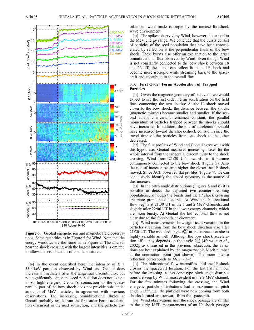
tributions were made isotropic by the intense foreshockwave environment.[30] The spikes observed by Wind, however, do extend to

the MeV energy range. We conclude that the bursts consistof particles of the seed population that have been reaccel-erated by reflection at the perpendicular flank of the bowshock. These bursts also offer an explanation to the largeromnidirectional flux observed by Wind. Even though Windis not constantly connected to the bow shock between 18and 22 UT, the bursts can reflect from the IP shock andbecome more isotropic while streaming back to the space-craft and contribute to the overall flux.

3.3. First Order Fermi Acceleration of TrappedParticles

[31] Given the magnetic geometry of the event, we wouldexpect to see the first order Fermi acceleration on the fieldlines connecting the two shocks: As the IP shock movedcloser to the bow shock, the distance between the shocks(magnetic mirrors) became smaller and smaller. If the sec-ond adiabatic invariant remained constant, the parallelmomentum of particles trapped between the shocks shouldhave increased. In addition, the rate of acceleration shouldhave increased toward the shock‐shock collision, since thetravel time of the particles from one shock to the otherdecreased.[32] The flux profiles of Wind and Geotail agree well with

this hypothesis. Geotail measured increasing fluxes for thewhole interval from the tangential discontinuity to the shockcrossing, Wind from 21:30 UT onwards, as it becamecontinuously connected to the bow shock (Figure 5). Alsothe rate of increase became higher the closer the IP shockmoved. Since ACE observed flat profiles (Figure 4), we canconclusively identify the closed geometry as the source ofthis increase.[33] In the pitch angle distributions (Figures 5 and 6) it is

possible to detect the expected two counter‐streamingpopulations, although the bursts and the IP shock crossingare more pronounced features. At Wind the bidirectionalflow begins at 21:30 UT in the 1 and 2 MeV channels, andslightly after 22:00 UT in the lower energy channels, whichare more bursty. At Geotail the bidirectional flow is notclear due to the foreshock environment.[34] Wind measurements show significant variation in the

particles streaming from the bow shock direction also after21:30 UT. The modeled angle �Bn

BS at the connection site ishighly variable as well. Although the bow shock accelera-tion efficiency depends on the angle �Bn

BS [Meziane et al.,2002], as discussed in the previous subsection, the varia-tions are best explained by the magnetosonic Mach numberat the connection point (not shown). The more intensereflection corresponds to MMS ∼ 3–5.[35] The bidirectional flow intensifies until the IP shock

crosses the spacecraft location. For the last half an hourbefore the crossing, a loss cone type pitch angle distribu-tions are seen by Wind, most evident in the 2 MeV channel.For the few minutes following the crossing, the Windenergetic particle distributions had a maximum at pitchangle ∼135°, i.e., the particles were now coming from bothshocks located antisunward from the spacecraft.[36] Wind observations near the shock passage are similar

to the early ISEE measurements of an IP shock passage

Figure 6. Geotail energetic ion and magnetic field observa-tions. Same quantities as in Figure 5 for Wind. Note that theenergy windows are the same as in Figure 2. The intervalnear the shock crossing with the largest intensities is omittedto allow the visualization of smaller features.


7 of 12

presented by Scholer and Ipavich [1983]. In their event,ISEE‐3 was located near the L1 point, while ISEE‐1 wasclose to the flank of the bow shock on the upstream side.The difference in the flux of low energy (30–157 keV) ionsbetween ISEE‐1 and 3 during the shock crossing is of thesame order of magnitude as between Wind and ACE in theevent studied here.

3.4. Acceleration Near the Intersection of the Shocks

[37] Let us consider the energetic particle observations ofGeotail during and immediately after the IP shock crossingat 00:41:48 UT. The increase in particle intensity (Figure 2)is significantly larger than at Wind, and the peak has adifferent structure as well: Figure 7 shows the flux intensi-ties between 00:35 UT and 00:50 UT on August 10. At lowenergies (E < 140 keV), the omnidirectional flux has itsmaximum 0–30 s before the shock crossing. Curiously, thehigher energy particles peak ∼2 min after the shock passage.[38] When we add directional information—the pitch

angle cosine m = cosa distributions shown in Figure 8 andthe flux of relevant sectors shown in Figure 7—we can seethat there are two separate maxima with magnitudesdepending on the energy channel. Particles propagating inthe magnetic field direction (purple lines in Figure 7) peakbefore the IP shock crossing. The gyrating ions with a ∼ 90°(not shown in Figure 7) have a maximum at the shockcrossing for low energy ions and up to 2 min after thecrossing for highest energies. They have very likely beenaccelerated at the IP shock.[39] The flux of particles propagating opposite to the

magnetic field direction (green lines in Figure 7) has amaximum at approximately 2 min after the shock at energiesfrom 61 keV to 1.4 MeV. In fact, at the 140–910 keV energyrange, the flux at these pitch angles is about as large as theflux at ∼90° pitch angles. Even at 910 keV–2 MeV, theanisotropy is still visible, but gyrating ions have signifi-cantly gained in relative intensity. Moreover, there seems tobe a velocity dispersion at these large pitch angles—higherenergy particles peaking before the lower energy particles—although this is at the limit of the temporal resolution of theinstrument (7 s for the lowest energy channels, 98 s for thehighest). As discussed below, we attribute this excess ofhigh energy, a ∼ 180°, particles to have been acceleratednear the intersection of the IP shock and the bow shock, towhich Geotail was magnetically connected for a short timeperiod.[40] Figure 9 illustrates the result of our modeling of the

IP shock propagation across the bow shock. For the positionand shape of the bow shock, we use the model proposed byMerka et al. [2005] with upstream solar wind data providedby IMP‐8 a few minutes before the IP shock crossing.IMP‐8 spent the longest time upstream of the IP shock, andwas not affected by the bow shock’s foreshock fluctuations.The location of the bow shock subsolar point is xnose =14.5−2.7

+3.5 RE and the intersection with the positive YGSE axisis ydusk = 29.1−1.9

+1.8 RE. In Figure 9, the upper limit has beendrawn as an orange mesh and the lower limit as a violetsurface. The magnetic field lines observed by Geotail (blacklines and green arrows), though fluctuating, were on averageconnected to the bow shock dusk flank. For the IP shock(cyan triangular planes), we use the IMP‐8 observation ofnIMP = (−0.72, −0.20, 0.66)GSE, since that particular part of

Figure 7. Geotail energetic particle fluxes near the IPshock passage from both north and south ion heads ofEPIC‐ICS and five different energy channels. As illus-trated by the inset giving the looking directions of thesectors, the (combined) average flux observed by sectors4, 5, and 6 (green) corresponds to particles with a pitchangle a ∼ 180°, while the flux of sectors 12, 13, and14 (purple) corresponds to a ∼ 0°. Black dashed linesshow the omnidirectional flux. The vertical dashed linesare the same as in Figure 8.


8 of 12

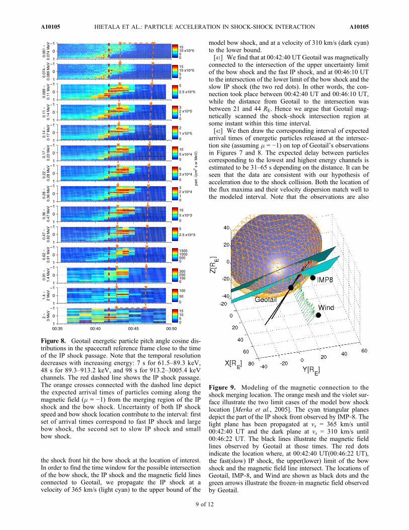
the shock front hit the bow shock at the location of interest.In order to find the time window for the possible intersectionof the bow shock, the IP shock and the magnetic field linesconnected to Geotail, we propagate the IP shock at avelocity of 365 km/s (light cyan) to the upper bound of the

model bow shock, and at a velocity of 310 km/s (dark cyan)to the lower bound.[41] We find that at 00:42:40 UT Geotail was magnetically

connected to the intersection of the upper uncertainty limitof the bow shock and the fast IP shock, and at 00:46:10 UTto the intersection of the lower limit of the bow shock and theslow IP shock (the two red dots). In other words, the con-nection took place between 00:42:40 UT and 00:46:10 UT,while the distance from Geotail to the intersection wasbetween 21 and 44 RE. Hence we argue that Geotail mag-netically scanned the shock‐shock intersection region atsome instant within this time interval.[42] We then draw the corresponding interval of expected

arrival times of energetic particles released at the intersec-tion site (assuming m = −1) on top of Geotail’s observationsin Figures 7 and 8. The expected delay between particlescorresponding to the lowest and highest energy channels isestimated to be 31–65 s depending on the distance. It can beseen that the data are consistent with our hypothesis ofacceleration due to the shock collision. Both the location ofthe flux maxima and their velocity dispersion match well tothe modeled interval. Note that the observations are also

Figure 8. Geotail energetic particle pitch angle cosine dis-tributions in the spacecraft reference frame close to the timeof the IP shock passage. Note that the temporal resolutiondecreases with increasing energy: 7 s for 61.5–89.3 keV,48 s for 89.3–913.2 keV, and 98 s for 913.2–3005.4 keVchannels. The red dashed line shows the IP shock passage.The orange crosses connected with the dashed line depictthe expected arrival times of particles coming along themagnetic field (m = −1) from the merging region of the IPshock and the bow shock. Uncertainty of both IP shockspeed and bow shock location contribute to the interval: firstset of arrival times correspond to fast IP shock and largebow shock, the second set to slow IP shock and smallbow shock.

Figure 9. Modeling of the magnetic connection to theshock merging location. The orange mesh and the violet sur-face illustrate the two limit cases of the model bow shocklocation [Merka et al., 2005]. The cyan triangular planesdepict the part of the IP shock front observed by IMP‐8. Thelight plane has been propagated at vs = 365 km/s until00:42:40 UT and the dark plane at vs = 310 km/s until00:46:22 UT. The black lines illustrate the magnetic fieldlines observed by Geotail at those times. The red dotsindicate the location where, at 00:42:40 UT(00:46:22 UT),the fast(slow) IP shock, the upper(lower) limit of the bowshock and the magnetic field line intersect. The locations ofGeotail, IMP‐8, and Wind are shown as black dots and thegreen arrows illustrate the frozen‐in magnetic field observedby Geotail.


9 of 12

consistent with the implication of our analysis that the fluxshould drop sharply after the arrival of these particles (seealso Figure 2), as the spacecraft lost its magnetic connectionto the IP shock that moved behind the bow shock.[43] A possible mechanism for the acceleration and

release of these particles is the collapse of the magnetic trapbetween the two shocks: Most of the particles are releasedfrom a magnetic bottle when its size decreases to the orderof a few gyroradii of the particles. According to our anal-ysis, this took place about one minute before the previouslydetermined intersection times on the field lines Geotail islocated. Since the gyroradius increases with the particleenergy, the higher energy particles will escape the trapbefore the lower energy ones. In our event, this would add afew tens of seconds to the velocity dispersion between theMeV and the 70‐keV particles. The increased dispersion andthe earlier release time are still compatible with the obser-vations. Moreover, the magnetic trap should be leakingalready before its collapse. The fact that the peaks of thea ∼ 180° particle flux have a certain width instead of beingstrictly spike‐like supports the collapsing trap interpretation.

3.5. Comparison of Energy Gain

[44] Given the data, it is evident that the particles influ-enced by both shocks gained more energy than the particlesaccelerated by the interplanetary shock only. We can esti-mate how much energy the seed population particles (seenby ACE) gained from the shock‐shock interaction processusing Liouville’s equation. We use the following approachsince the observed spectrum of the energetic particles isquite featureless, i.e., there is no pronounced feature whosepropagation we could follow.[45] According to the Liouville’s equation df/dt = 0, i.e.,

the value of the distribution function f stays constant fol-lowing the motion of the particles:

f r; v; tð Þ ¼ f r0; v0; t0ð Þ: ð1Þ

Here r = r(t; r0, v0, t0) and v = v(t; r0, v0, t0) give the tra-jectory of the particles in phase space defined by the initialvalues r0, v0, and t0.[46] Let us assume that, at a certain time, we observe at a

given momentum pa an amount of particles given by thevalue of the distribution function f = fa. At a later time, theobserved amount at the same momentum has increased to fb.According to equation (1), these particles should originatefrom that part of the phase space where the population hadthe same value of the distribution function as the observedone. Therefore, if the spectrum of the particles is given byf ∼ p−g, we can estimate that the particles fb were acceleratedfrom a lower momentum pb, so that

log10papb

� �¼ �1

�log10

fafb

� �: ð2Þ

Using the energy E ∼ p2 and the flux intensity I ∼ p2 finstead,

log10Ea

Eb

� �¼ �2

� � 2log10

IaIb

� �: ð3Þ

Thus, given the spectral index g and the increase in intensitywith respect to the seed population of the IP shock, we cancalculate the energy Ea of the particles that have undergoneshock‐shock interaction, in terms of the energy of the seedpopulation Eb.[47] Naturally, this approach is unsuitable if there are

other sources of energetic particles. In the event describedhere, however, the leakage from the magnetosphere isunlikely due to the very quiet conditions (Dst between−25 nT and −5 nT, AE ] 100 nT).[48] Figure 10 shows the spectra of energetic ions mea-

sured by the different spacecraft right after the tangentialdiscontinuity (plus signs), and at the IP shock crossing(circles). The Geotail spectrum at the peak intensity is alsoshown (crosses). ACE observations stayed almost constantwith the spectral index in momentum g ∼ 8. This staticnature is consistent with our previous discussion concerningthe weakness of the IP shock. The spectra from Wind andGeotail after the TD were very close those of ACE, asexpected. At the IP shock crossing, these had shifted to theright, as the particles had gained energy from the shock‐shock interaction. The spectrum measured by Geotail wassomewhat softer than before.

Figure 10. The measured spectra of energetic ions plottedas distribution function f versus momentum p. ACE obser-vations in red, Wind in blue, and Geotail in two shades ofgreen. Plus signs correspond to measurements right afterthe tangential discontinuity, while circles correspond to theinterplanetary shock crossing. Crosses correspond to the peakintensity at Geotail ∼2 minutes after the IP shock crossing.The dashed line of p−8 is drawn to guide the eye.


10 of 12

[49] In order to the estimate the energy gain, let us con-sider the energy channels in the range 0.2–2 MeV. Wedenote the seed population energies by EA, as they are givenby ACE flux measurements after the TD. We estimate(equation (3)) that the flux maxima observed by Wind at theIP shock crossing correspond to the energy of the particleshaving increased to ∼1.5 EA in all channels. At the intensitypeak measured by Geotail shortly after the IP shock crossingthe increase was ∼3 EA in the lower channels and ∼2 EA inthe higher channels.[50] When the IP shock crossed Wind, the particles

trapped between the shocks were undergoing first orderFermi acceleration. Yet the shocks were still quite far apart—tens of ion gyroradii—so the energy gain was relativelysmall. However, Geotail observed the particles as they werereleased from the magnetic trap between the shocks. Weconclude that the energy of the particles escaping from thecollapsing trap was 2–3 times higher than of those inter-acting only with a single shock.

4. Discussion and Conclusions

[51] Previous observations of particle acceleration inshock‐shock collisions have been mostly indirect; theinteraction of CMEs, for instance, has usually been inferredby combining LASCO white‐light coronagraph images withradio observations (for a recent summary, see, e.g., Lugazet al. [2008]). In the chromosphere, Narukage et al. [2008]have discovered three successive Moreton waves generatedby a single flare using Ha images. The second shock caughtup with the first and merged with it. Similarly to CMEinteraction studies, the collision between the Moreton waveswas accompanied by a sudden enhancement of the radiosignal. However, pointing out the exact source region of theradio emissions in this manner is very difficult [Reiner et al.,2003; Richardson et al., 2003].[52] In the event described by Scholer and Ipavich [1983]

[see also Kennel et al., 1984], the magnetic geometry wasdifferent from the one studied here: First, the change in theIMF direction at the IP shock was large, from quasi‐radial tosouthward. Second, the ISEE‐1 spacecraft was very close tothe bow shock and on the dawn flank. In fact, ISEE‐1 wasnot connected to the bow shock during the half hour fol-lowing the IP shock crossing. Consequently, it was notpossible to observe particles accelerated at the shock‐shockintersection. To our knowledge, we report the first direct,in situ measurements of accelerated particles that have beenreleased from a magnetic trap but a moment before the twospace plasma shocks collided.[53] Gómez‐Herrero et al. [2011] have recently reported

on STEREO observations of several CIR events, where anICME was observed near the CIR by one of the space-craft, but not by the other. The differences of the maximumhundred‐keV range energetic particle flux intensities betweenthe spacecraft were typically 1–2 orders of magnitude. In theobserved interaction events, either one or both of the CIRshocks had formed already at 1 AU, and in some events theflux maxima could be associated with these. However, insome of the events, neither shocks nor developing shockscould be related to the maxima. Based on our measurementsof the enhanced particle acceleration, we propose thatthese latter flux maximum differences, similar in magnitude

compared to ours, could be signals of interaction (trappingof particles) between the CIR and the ICME shocks beyond1 AU. Naturally, a more detailed analysis of global (mag-netic) geometry of the events would be required to verifythis.[54] In summary, we have presented detailed multispace-

craft observations of the interaction between a weak IPshock and the bow shock of the Earth during quasi‐radialIMF geometry. After crossing a tangential discontinuity, thespacecraft moved into a flux tube that was filled with a seedpopulation of energetic particles accelerated by the IP shock.Since ACE was connected to the IP shock but not to the bowshock during the event, the seed population could be char-acterized by its measurements. A notable feature was theflatness of the flux intensity profiles for the whole intervalfrom the TD crossing to the IP shock crossing.[55] During the first part of the event, Wind at XGSE ∼

78 RE observed several particle bursts of up to a few MeVscoming from the bow shock direction. According to ouranalysis, the spacecraft was connected to the quasi‐perpendicular part of the bow shock at these times, so thebursts consisted of particles of the seed population that hadundergone reflection at the connection point. Later, thespacecraft became continuously connected to the bowshock, and measured an increasing flux until the IP shockcrossing, as the particles trapped between the two shockswere undergoing Fermi acceleration.[56] Geotail was located closest to the Earth and was near

the edge of or within the foreshock of the bow shock. Sinceit was inside the magnetic trap between the two shocks forthe longest period of time, the measured flux increase andpeak intensity were the highest. Furthermore, immediatelyafter the IP shock crossing Geotail observed a burst of veryhigh energy particles propagating sunwards. Based on thevelocity dispersion of the burst and our analysis of thegeometry of the two shocks, we claim that these particleshad been released from the trap as the shocks collided. Wealso estimate that the shock‐shock interaction had increasedtheir energy to 2–3 times the energy of the seed populationproduced by the IP shock.

[57] Acknowledgments. We thank CDAWeb at NSSDC for dataaccess and the PIs of the different instruments. We wish to thank theACE and Wind teams for making the data available. Geotail high resolutionmagnetic field data were provided by T. Nagai through DARTS at Instituteof Space and Astronautical Science, JAXA in Japan. H.H. would like tothank T. Koskela for data analysis tips. The work of H.H. was supportedby the Väisälä foundation. The work of N.A. was partially supported byNASA grants NNX08AE34G and NAS5‐98033. The work of K.A. andE.K. was supported by the Academy of Finland.

ReferencesBurgess, D., et al. (2005), Quasi‐parallel shock structure and processes,Space Sci. Rev., 118, 205–222.

Burlaga, L. F. (1993), Solar wind behavior throughout the heliosphere, Adv.Space Res., 13(6), 27–35.

Cargill, P. J. (1991), The interaction of collisionless shocks in astrophysicalplasmas, Astrophys. J., 376, 771–781.

Desai, M. I., G. M. Mason, R. Müller‐Mellin, A. Korth, U. Mall,J. R. Dwyer, and T. T. von Rosenvinge (2008), The spatial distributionof upstream ion events from the Earth’s bow shock measured by ACE,Wind, and STEREO, J. Geophys. Res., 113, A08103, doi:10.1029/2007JA012909.

Dudkin, G. N., A. A. Lukanin, B. A. Nechaev, A. V. Peshkov, andV. A. Ryzhkov (1992), Observation of deuteron acceleration in a collision


11 of 12

of magnetosonic shock waves in a plasma, Pis’ma Zh. Eksp. Teor. Fiz.,55, 689–691.

Dudkin, G. N., V. Y. Egorov, B. A. Nechaev, and A. V. Peshkov (1995),Mechanism for ion acceleration in a collision of magnetosonic shockwaves, Pis’ma Zh. Eksp. Teor. Fiz., 61, 617–620.

Gold, R. E., S. M. Krimigis, S. E. Hawkins, D. K. Haggerty, D. A. Lohr,E. Fiore, T. P. Armstrong, G. Holland, and L. J. Lanzerotti (1998), Elec-tron, proton, and alpha monitor on the Advanced Composition Explorerspacecraft, Space Sci. Rev., 86, 541–562.

Gómez‐Herrero, R., O. Malandraki, N. Dresing, E. Kilpua, B. Heber,A. Klassen, R. Müller‐Mellin, and R. F. Wimmer‐Schweingruber(2011), Spatial and temporal variations of CIRs: Multi‐point observationsby STEREO, J. Atmos. Sol. Terr. Phys., 73, 551–565.

Jian, L., C. T. Russel, J. G. Luhmann, and R. M. Skoug (2006), Propertiesof interplanetary coronal mass ejections at one AU during 1995–2004,Sol. Phys., 239, 393–436.

Kennel, C. F., et al. (1984), Plasma and energetic particle structureupstream of a quasi‐parallel interplanetary shock, J. Geophys. Res., 89,5419–5435.

Lembège, B., Y. Ma, and X. Deng (2010), Collision of two supercriticalquasi‐perpendicular nonstationary collisionless shocks: Full particlesimulations, Abstract SM51B‐1790 presented at 2010 Fall Meeting,AGU, San Francisco, Calif., 13–17 Dec.

Lin, R. P., et al. (1995), A three‐dimensional plasma and energetic particleinvestigation for the Wind spacecraft, Space Sci. Rev., 71, 125–153.

Lugaz, N., W. B. Manchester IV, I. I. Roussev, and T. I. Gombosi (2008),Observational evidence of CMEs interacting in the inner heliosphere asinferred from MHD simulations, J. Atmos. Sol. Terr. Phys., 70, 598–604.

Matthaeus, W., M. Goldstein, and J. King (1986), An interplanetary mag-netic field ensemble at 1 AU, J. Geophys. Res., 91(A1), 59–69.

Merka, J., A. Szabo, J. A. Slavin, and M. Peredo (2005), Three‐dimensionalposition and shape of the bow shock and their variation with upstreamMach numbers and interplanetary magnetic field orientation, J. Geophys.Res., 110, A04202, doi:10.1029/2004JA010944.

Meziane, K., R. P. Lin, G. K. Parks, D. E. Larson, S. D. Bale, G. M.Mason, J. R. Dwyer, and R. P. Lepping (1999), Evidence for accelerationof ions to ∼1 MeV by adiabatic‐like reflection at the quasi‐perpendicularEarth’s bow shock, Geophys. Res. Lett., 26, 2925–2928.

Meziane, K., A. J. Hull, A. M. Hamza, and R. P. Lin (2002), On thebow shock �Bn dependence of upstream 70 keV to 2 MeV ion fluxes,J. Geophys. Res., 107(A9), 1243, doi:10.1029/2001JA005012.

Narukage, N., T. T. Ishii, S. Nagata, S. UeNo, R. Kitai, H. Kurokawa,M. Akioka, and K. Shibata (2008), Three successive and interactingshock waves generated by a solar flare, Astrophys. J., 684, L45–L49.

Omidi, N., D. G. Sibeck, and X. Blanco‐Cano (2009), Foreshock com-pressional boundary, J. Geophys. Res., 114, A08205, doi:10.1029/2008JA013950.

Prech, L., Z. Nemecek, and J. Safrankova (2009), Influence of the fore-shock of the Earth’s bow shock on the interplanetary shock propagationduring their mutual interaction, Earth Planets Space, 61, 607–610.

Priest, E. R. (1984), Solar Magnetohydrodynamics, Springer, Dordrecht,Netherlands.

Reiner, M. J., A. Vourlidas, O. C. S. Cyr, J. T. Burkepile, R. A. Howard,M. L. Kaiser, N. P. Prestage, and J.‐L. Bougeret (2003), Constraints oncoronal mass ejection dynamics from simultaneous radio and white‐lightobservations, Astrophys. J., 590, 533–546.

Richardson, I. G., G. R. Lawrence, D. K. Haggerty, T. A. Kucera, andA. Szabo (2003), Are CME “interactions” really important for accelerat-ing major solar energetic particle events?, Geophys. Res. Lett., 30(12),8014, doi:10.1029/2002GL016424.

Sandroos, A., and R. Vainio (2009), Reacceleration of flare ions in coronaland interplanetary shock waves, Astrophys. J. Suppl. Ser., 181, 183–196.

Scholer, M., and F. M. Ipavich (1983), Energetic ions upstream of theEarth’s bow shock during an energetic storm particle event, J. Geophys.Res., 88, 5715–5726.

Stone, R. G., and B. T. Tsurutani (Eds.) (1985), Collisionless Shocks in theHeliosphere: A Tutorial Review, Geophys. Monogr. Ser., vol. 34, AGU,Washington, D. C.

Szabo, A. (2005), Determination of interplanetary shock characteristics,in “Connecting Sun and Heliosphere”: Proceedings of Solar Wind11/SOHO 16, edited by B. Fleck and T. H. Zurbuchen, Eur. SpaceAgency Spec. Publ., ESA SP‐592, 449–452.

Terasawa, T., et al. (1997), Particle acceleration at the interplanetary shockahead of a large magnetic cloud on October 18, 1995: GEOTAIL‐WINDcollaboration, Adv. Space Res., 20, 641–644.

Williams, D. J., R. W. McEntire, C. I. Schlemm, A. T. Y. Lui, G. Gloeckler,S. P. Christon, and F. Gliem (1994), GEOTAIL energetic particles andion composition instrument, J. Geomagn. Geoelectr., 46, 39–57.

N. Agueda, Departament d’Astronomia i Meteorologia, Institut deCiències del Cosmos, Universitat de Barcelona, Martí i Franquès, 1,E‐08028 Barcelona, Spain.K. Andréeová, H. Hietala, E. K. J. Kilpua, H. E. J. Koskinen, and

R. Vainio, Department of Physics, University of Helsinki, P.O. Box 64,FI‐00014 Helsinki, Finland. ([email protected])S. Nylund, Applied Physics Laboratory, Johns Hopkins University, M.S.

Bldg 7‐314, 11100 Johns Hopkins Rd, Laurel, MD 20723‐6099, USA.


12 of 12

in situ observations of particle acceleration in shock ...blai/articles/11hietalaetal_jgr.pdfh....

Documents