incorporating a dynamic irrigation demand module into an integrated surface water/groundwater model...

Incorporating a Dynamic Irrigation Demand Module into an Integrated Surface

Water/Groundwater Model to Assess Drought Response

Dirk Kassenaar, E.J. Wexler

Peter J. Thompson, Michael Takeda

Toward Sustainable Groundwater in Agriculture

San Francisco, CA

June 30, 2016

Presentation Outline

1. Background: Source Water Protection in Ontario, Canada

2. Dynamic irrigation demand and consumptive use

3. Integrated SW/GW Modelling

4. Pilot Watershed: Source Water Protection Study/ Low Water Response

Project

5. GSFLOW Code modifications and conceptual testing

6. Simulation of farm operations in study sub watershed Conclusions

Integrated Simulation of Irrigation Demand - Introduction 2

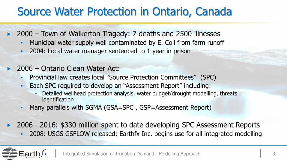
Source Water Protection in Ontario, Canada

2000 – Town of Walkerton Tragedy: 7 deaths and 2500 illnesses ▪ Municipal water supply well contaminated by E. Coli from farm runoff

▪ 2004: Local water manager sentenced to 1 year in prison

2006 – Ontario Clean Water Act: ▪ Provincial law creates local “Source Protection Committees” (SPC)

▪ Each SPC required to develop an “Assessment Report” including: • Detailed wellhead protection analysis, water budget/drought modelling, threats

identification

▪ Many parallels with SGMA (GSA=SPC , GSP=Assessment Report)

2006 - 2016: $330 million spent to date developing SPC Assessment Reports ▪ 2008: USGS GSFLOW released; Earthfx Inc. begins use for all integrated modelling

Integrated Simulation of Irrigation Demand - Modelling Approach 3

Agricultural Water Use

Irrigation in Ontario is growing in response to: ▪ Increase in climate variability

▪ Contract farming: “Supply chain” management approach and need for production certainty • Contractual obligation to irrigate throughout the growing season

▪ Advances in precision agriculture

Irrigation operations ▪ Shift from SW sources to GW sources both for supply certainty and ecosystem protection

▪ Regulators looking for modelling tools and insights for better permit allocation and water use monitoring

Need to comprehensively simulate “soil moisture-based irrigation water use” ▪ Consumptive use assessment: GW pumping, ET losses, enhanced runoff, GW return flow,

changes in baseflow, induced stream losses, etc.


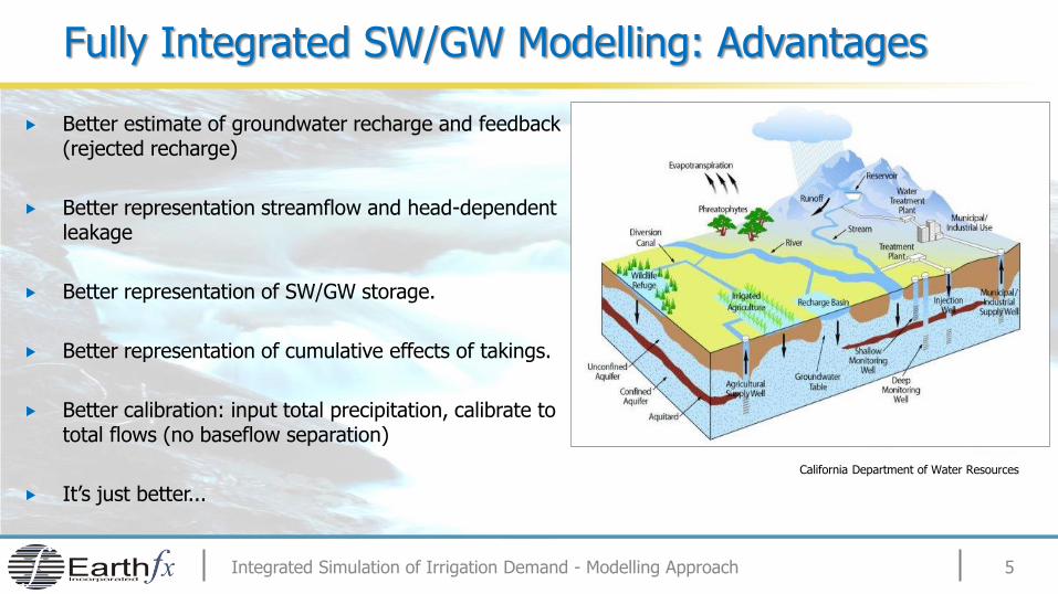
Fully Integrated SW/GW Modelling: Advantages

Better estimate of groundwater recharge and feedback (rejected recharge)

Better representation streamflow and head-dependent leakage

Better representation of SW/GW storage.

Better representation of cumulative effects of takings.

Better calibration: input total precipitation, calibrate to total flows (no baseflow separation)

It’s just better...


California Department of Water Resources

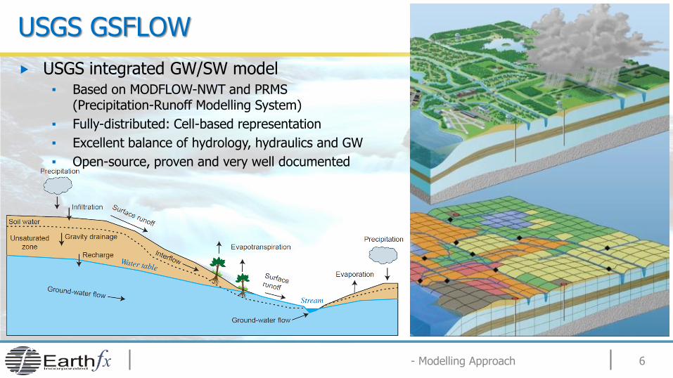
USGS GSFLOW

USGS integrated GW/SW model ▪ Based on MODFLOW-NWT and PRMS

(Precipitation-Runoff Modelling System)

▪ Fully-distributed: Cell-based representation

▪ Excellent balance of hydrology, hydraulics and GW

▪ Open-source, proven and very well documented

6 - Modelling Approach

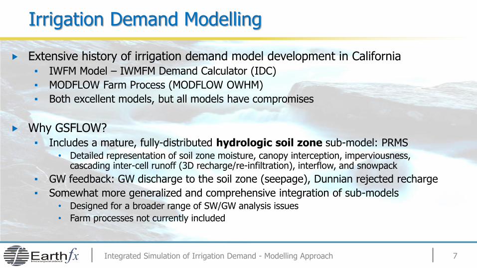
Irrigation Demand Modelling

Extensive history of irrigation demand model development in California ▪ IWFM Model – IWMFM Demand Calculator (IDC)

▪ MODFLOW Farm Process (MODFLOW OWHM)

▪ Both excellent models, but all models have compromises

Why GSFLOW? ▪ Includes a mature, fully-distributed hydrologic soil zone sub-model: PRMS

• Detailed representation of soil zone moisture, canopy interception, imperviousness, cascading inter-cell runoff (3D recharge/re-infiltration), interflow, and snowpack

▪ GW feedback: GW discharge to the soil zone (seepage), Dunnian rejected recharge

▪ Somewhat more generalized and comprehensive integration of sub-models • Designed for a broader range of SW/GW analysis issues

• Farm processes not currently included


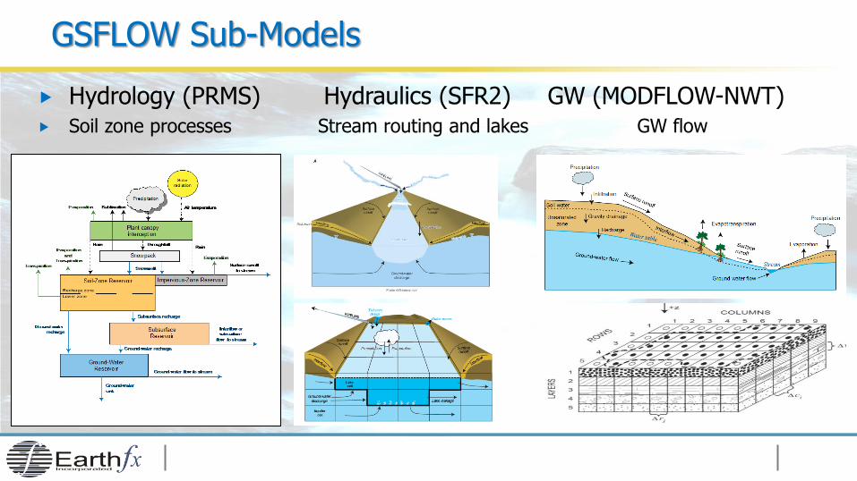
GSFLOW Sub-Models

Hydrology (PRMS) Hydraulics (SFR2) GW (MODFLOW-NWT) Soil zone processes Stream routing and lakes GW flow

GSFLOW Spatial and Temporal Resolution

Spatial resolution: Three grid definitions for climate, soils and GW system

▪ We typically use a soil zone resolution 10 to 100 times finer resolution to represent

Temporal resolution: Daily time step for groundwater, option for hourly climate-driven processes

9 - Modelling Approach

Climate: NEXRAD Precip. Soils: LIDAR, MODIS, ELC land use, remote sensing data GW: Variable cell MODFLOW grid

PILOT WATERSHED - STUDY SUB WATERSHED

Integrated Simulation of Irrigation Demand – Watershed Overview 10

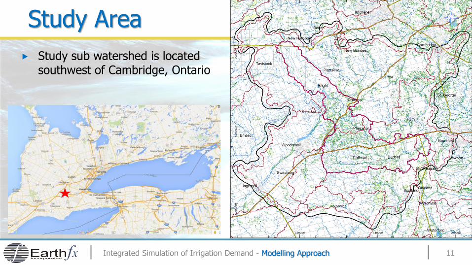
Study Area

Study sub watershed is located southwest of Cambridge, Ontario


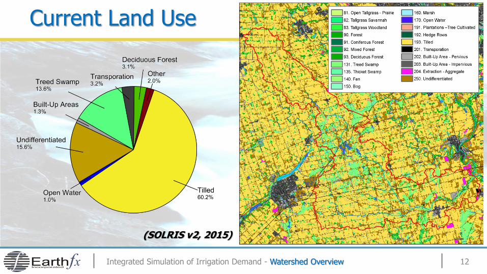
Current Land Use

12 Integrated Simulation of Irrigation Demand - Watershed Overview

(SOLRIS v2, 2015)

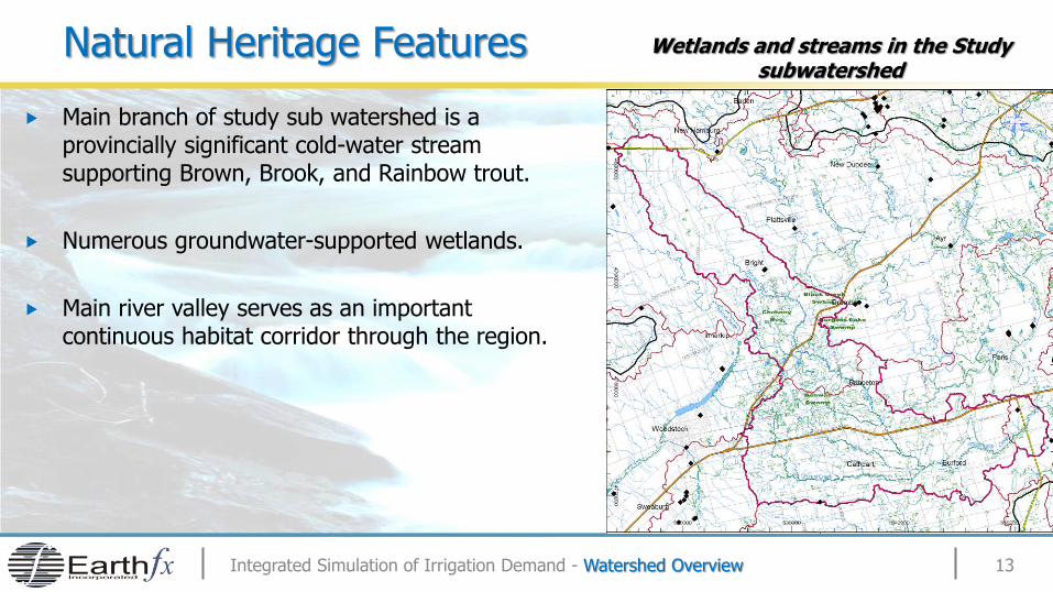
Main branch of study sub watershed is a provincially significant cold-water stream supporting Brown, Brook, and Rainbow trout.

Numerous groundwater-supported wetlands.

Main river valley serves as an important continuous habitat corridor through the region.

Wetlands and streams in the Study subwatershed

Natural Heritage Features

Integrated Simulation of Irrigation Demand - Watershed Overview 13

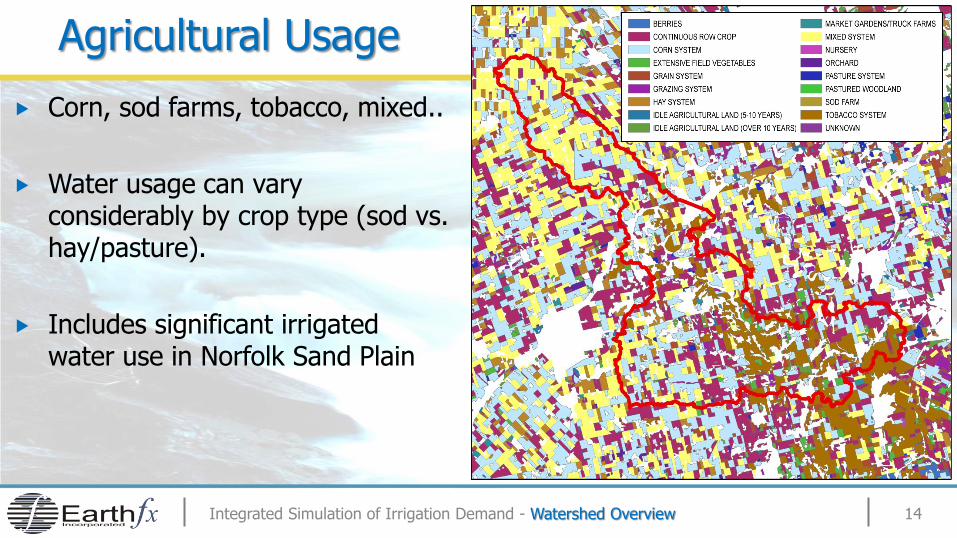
Agricultural Usage

14

Corn, sod farms, tobacco, mixed..

Water usage can vary considerably by crop type (sod vs. hay/pasture).

Includes significant irrigated water use in Norfolk Sand Plain

Integrated Simulation of Irrigation Demand - Watershed Overview

Integrated Simulation of Irrigation Demand - Geologic & Hydrostratigraphic Model 15

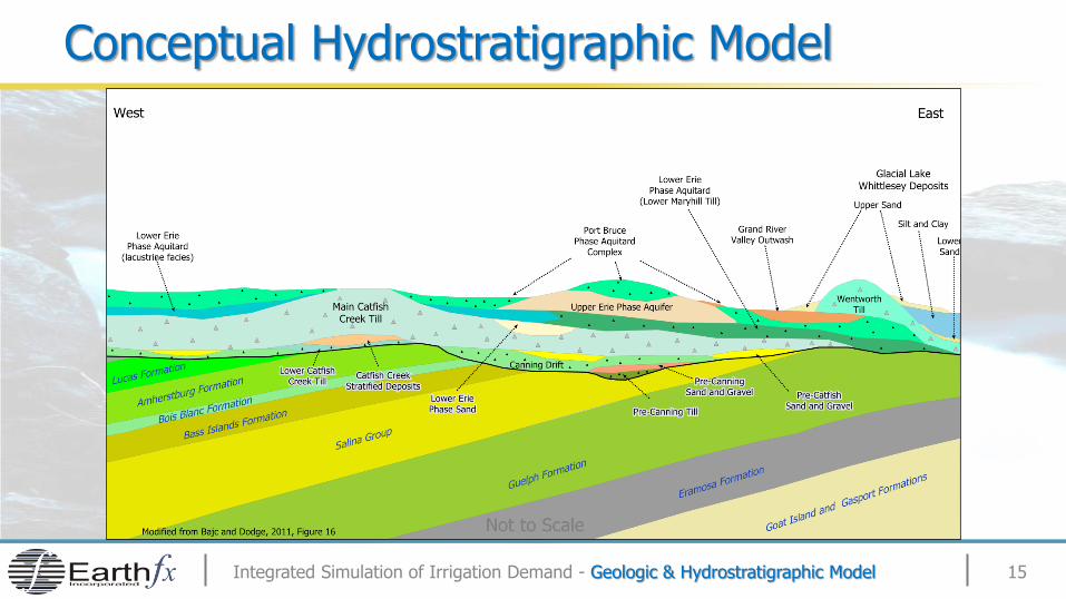
Conceptual Hydrostratigraphic Model

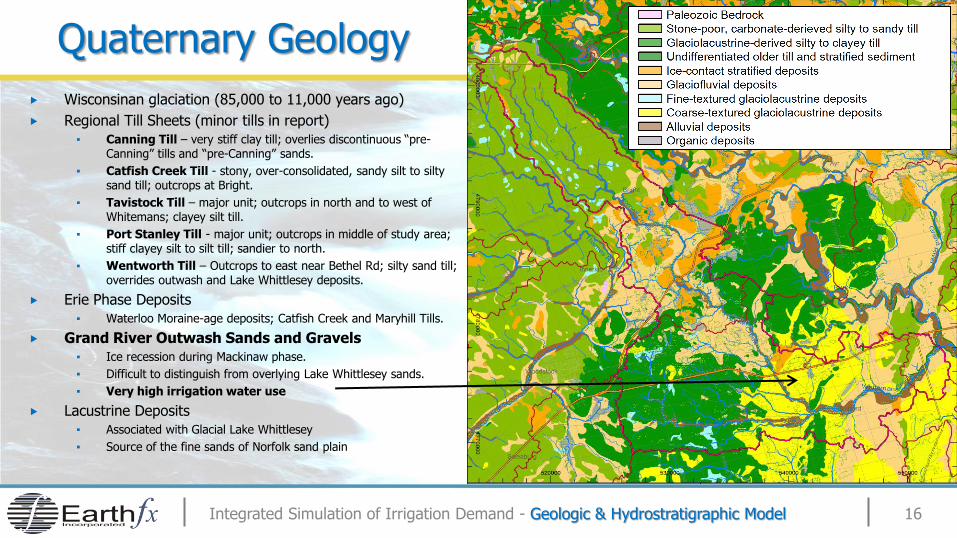
Wisconsinan glaciation (85,000 to 11,000 years ago)

Regional Till Sheets (minor tills in report) ▪ Canning Till – very stiff clay till; overlies discontinuous “pre-

Canning” tills and “pre-Canning” sands.

▪ Catfish Creek Till - stony, over-consolidated, sandy silt to silty sand till; outcrops at Bright.

▪ Tavistock Till – major unit; outcrops in north and to west of Whitemans; clayey silt till.

▪ Port Stanley Till - major unit; outcrops in middle of study area; stiff clayey silt to silt till; sandier to north.

▪ Wentworth Till – Outcrops to east near Bethel Rd; silty sand till; overrides outwash and Lake Whittlesey deposits.

Erie Phase Deposits

▪ Waterloo Moraine-age deposits; Catfish Creek and Maryhill Tills.

Grand River Outwash Sands and Gravels ▪ Ice recession during Mackinaw phase.

▪ Difficult to distinguish from overlying Lake Whittlesey sands.

▪ Very high irrigation water use

Lacustrine Deposits

▪ Associated with Glacial Lake Whittlesey

▪ Source of the fine sands of Norfolk sand plain

Integrated Simulation of Irrigation Demand - Geologic & Hydrostratigraphic Model 16

Quaternary Geology

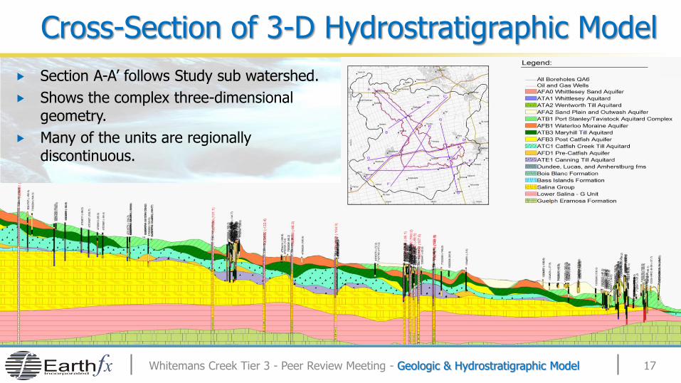
Section A-A’ follows Study sub watershed.

Shows the complex three-dimensional geometry.

Many of the units are regionally discontinuous.

Whitemans Creek Tier 3 - Peer Review Meeting - Geologic & Hydrostratigraphic Model 17

Cross-Section of 3-D Hydrostratigraphic Model

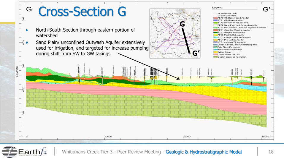
North-South Section through eastern portion of watershed

Sand Plain/ unconfined Outwash Aquifer extensively used for irrigation, and targeted for increase pumping during shift from SW to GW takings

Whitemans Creek Tier 3 - Peer Review Meeting - Geologic & Hydrostratigraphic Model 18

Cross-Section G G

G’

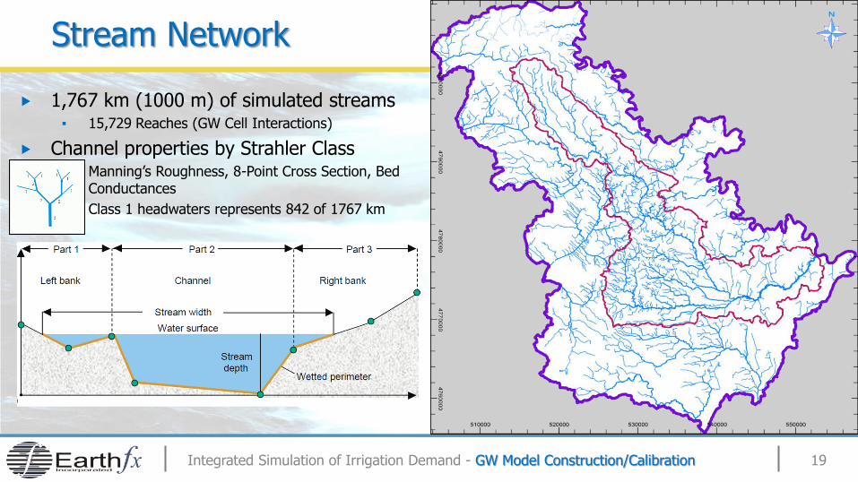
Stream Network

Integrated Simulation of Irrigation Demand - GW Model Construction/Calibration 19

1,767 km (1000 m) of simulated streams ▪ 15,729 Reaches (GW Cell Interactions)

Channel properties by Strahler Class ▪ Manning’s Roughness, 8-Point Cross Section, Bed

Conductances

▪ Class 1 headwaters represents 842 of 1767 km

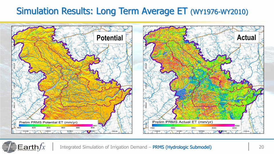
Simulation Results: Long Term Average ET (WY1976-WY2010)

Integrated Simulation of Irrigation Demand – PRMS (Hydrologic Submodel) 20

Potential Actual

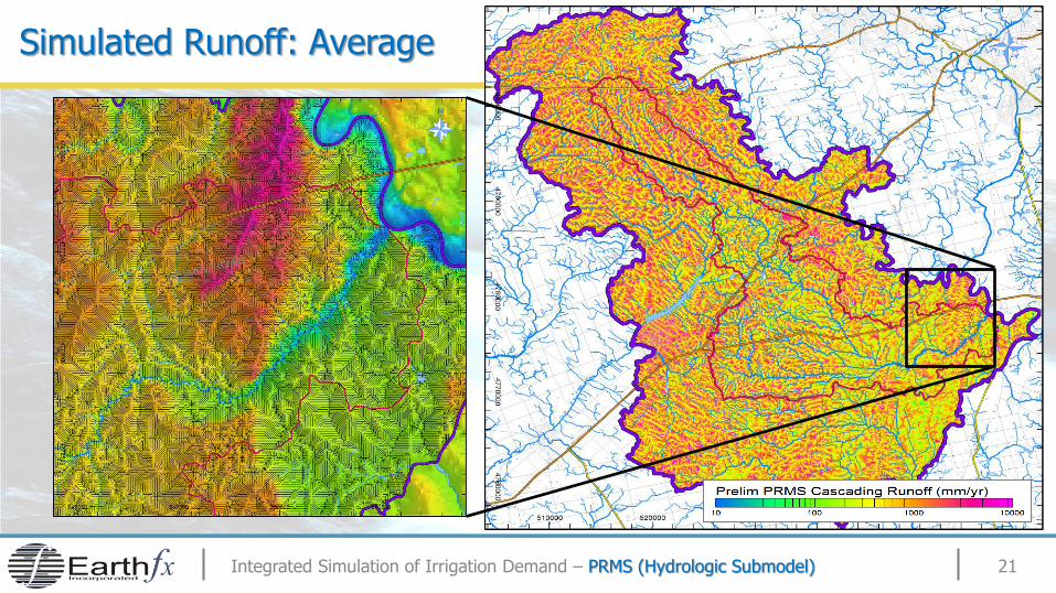
Simulated Runoff: Average


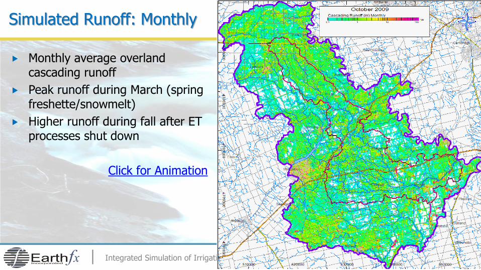
Simulated Runoff: Monthly

Monthly average overland cascading runoff

Peak runoff during March (spring freshette/snowmelt)

Higher runoff during fall after ET processes shut down

Click for Animation


https://youtu.be/ypa2YLL5So0?t=1m45s

Simulated Runoff: Daily

23

Click for Animation


24

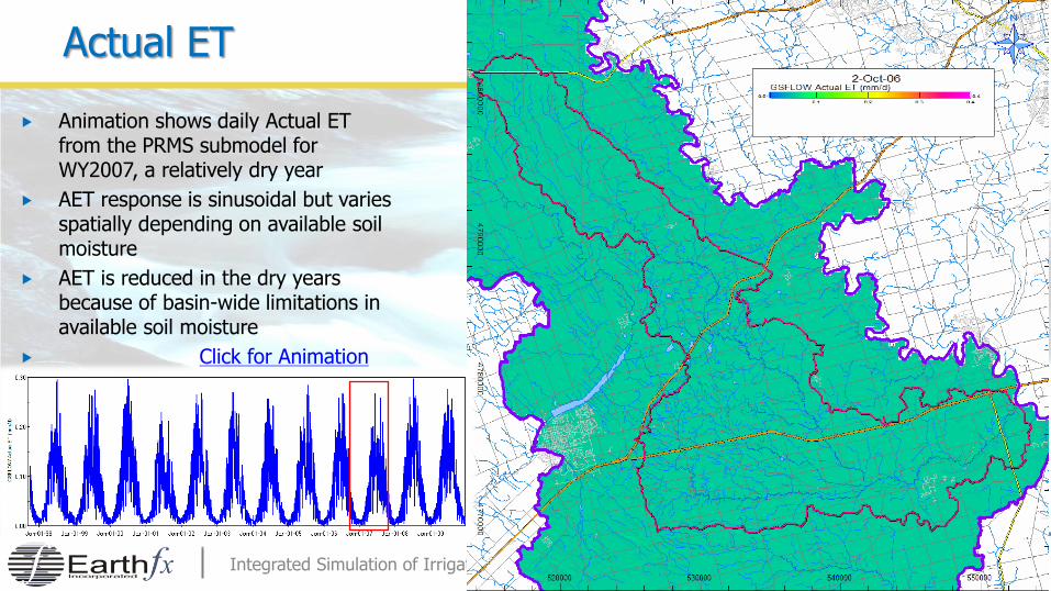
Actual ET

Integrated Simulation of Irrigation Demand – Preliminary GSFLOW Model Calibration

Animation shows daily Actual ET from the PRMS submodel for WY2007, a relatively dry year

AET response is sinusoidal but varies spatially depending on available soil moisture

AET is reduced in the dry years because of basin-wide limitations in available soil moisture

Click for Animation


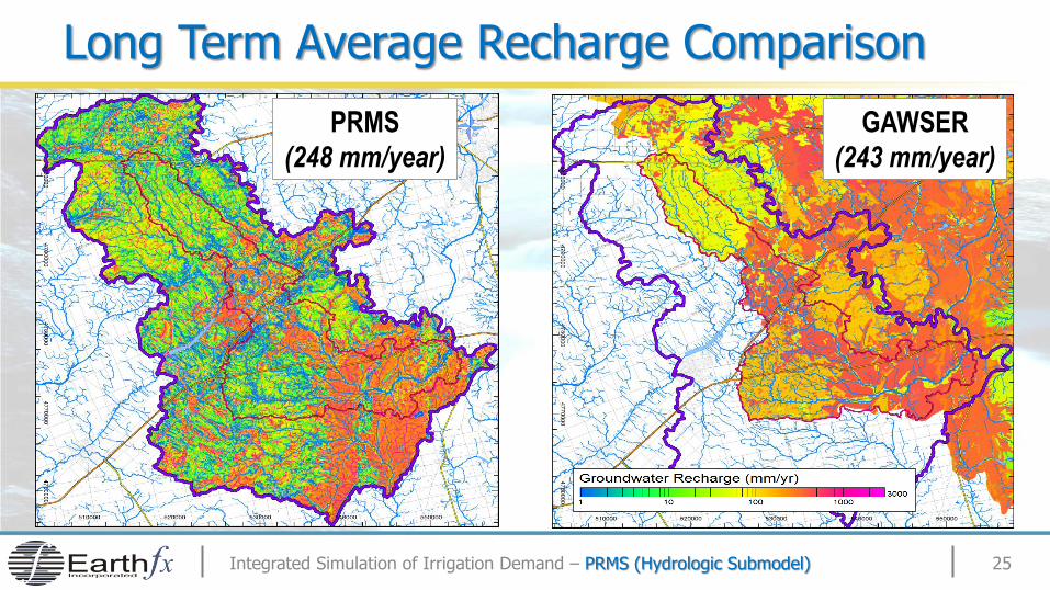
Long Term Average Recharge Comparison


PRMS

(248 mm/year)

GAWSER

(243 mm/year)

26

Water Levels


Animation shows transient water levels from the MODFLOW submodel in Layer 3 for WY2007

Groundwater response appears muted because of contour interval places but change is in range of 1-2 metres

Click for Animation


27

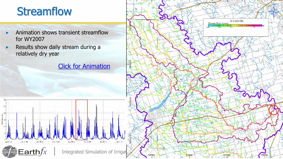
Streamflow


Animation shows transient streamflow for WY2007

Results show daily stream during a relatively dry year

Click for Animation


28

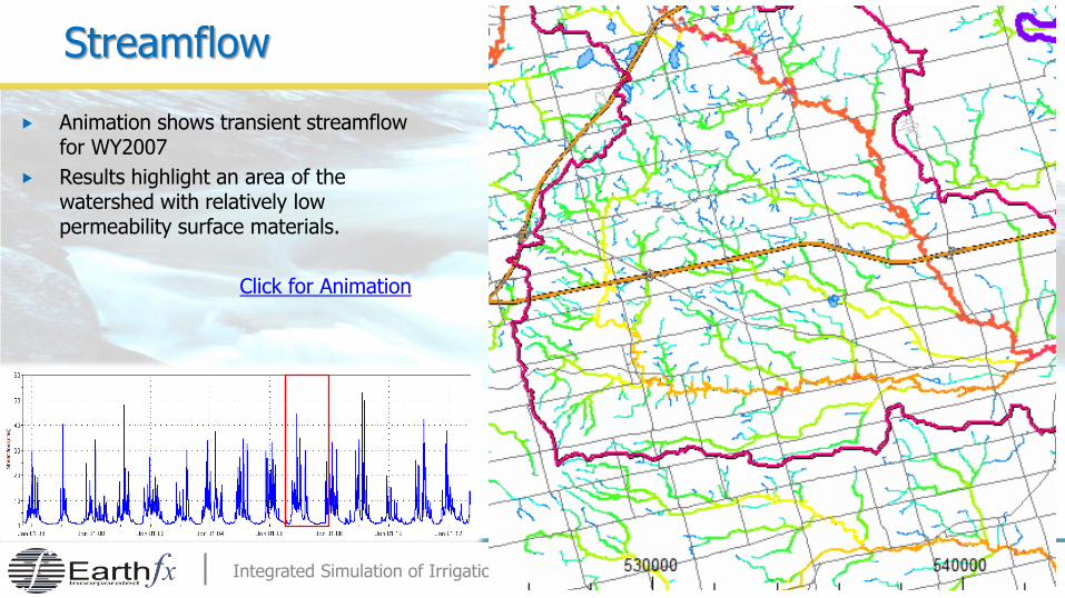
Streamflow


Animation shows transient streamflow for WY2007

Results highlight an area of the watershed with relatively low permeability surface materials.

Click for Animation


A total of 470 permitted GW takings located in the study area

Integrated Simulation of Irrigation Demand - Water Use 29

GW Pumping

SW Diversions

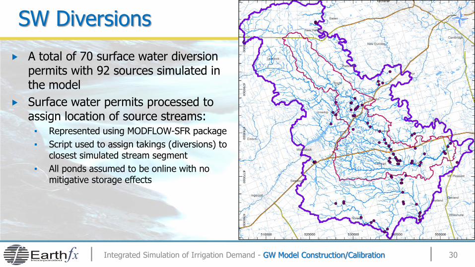
Integrated Simulation of Irrigation Demand - GW Model Construction/Calibration 30

A total of 70 surface water diversion permits with 92 sources simulated in the model

Surface water permits processed to assign location of source streams: ▪ Represented using MODFLOW-SFR package

▪ Script used to assign takings (diversions) to closest simulated stream segment

▪ All ponds assumed to be online with no mitigative storage effects

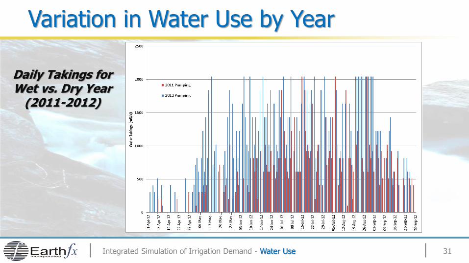
Daily Takings for Wet vs. Dry Year

(2011-2012)


Variation in Water Use by Year

Study Sub Watershed GSFLOW Model

Results present the current coarse model resolution (240m cell size) preliminary calibration

All components of the hydrologic cycle are represented and functioning

Simulation of irrigation demand necessary for final calibration and water budget assessment under drought conditions


SOIL MOISTURE DEMAND-BASED IRRIGATION MODULE

Earthfx GSFLOW Code Extension

Integrated Simulation of Irrigation Demand - Streamflow Data 33

Irrigation Module for GSFLOW

Earthfx Inc. has developed a new irrigation module for GSFLOW

The general technical approach is based on work by the USGS for the simulation of water use in California’s Central Valley

▪ Based on MODFLOW-OWHM and the “Farm Process” module

▪ While functionally similar to OWHM, the new GSFLOW module uses PRMS soil zone hydrologic parameter and processes

Testing and implementation support funding provided by the the Ontario MNR, MOECC and Grand River Conservation Authority


Simulation of Soil Moisture-based Agricultural Water Use

Simulation of irrigation (GW or SW diversions) based on soil moisture levels:

▪ Pumping representation in the model is only the start:

• Need to estimate consumptive use

▪ Water applied as precipitation (spray irrigation) or after canopy interception (drip)

▪ Losses of irrigation water to ET or enhanced runoff to streams

▪ Return flows – irrigation water re-infiltrates, but not necessarily to the same aquifer

▪ Induced changes in stream interaction

Applications of moisture demand-based simulations:

▪ Can be used to estimate actual historic consumptive water use

▪ Evaluation of projected water use under future drought

▪ Climate change conditions: earlier spring means longer summer GW level recession


Irrigation Demand Submodel - Methodology

General methodology to estimate water use requires daily takings:

▪ GSFLOW/PRMS daily estimate of soil moisture used to “trigger” irrigation.

▪ Irrigation starts when available soil moisture falls below trigger

▪ Trigger can be defined based on soil and crop type

▪ Irrigation water can be lost to ET, runoff or returned to the GW system

▪ Impacts of GW pumping or SW diversions fully represented

Predictive irrigation submodel can be calibrated to actual water use data, or used to estimate historical, current or future water use


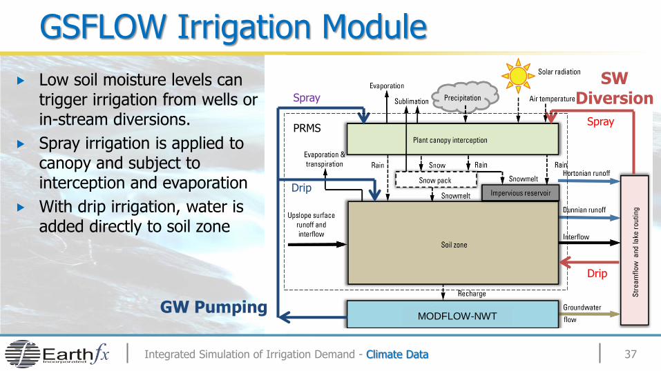
GSFLOW Irrigation Module

Low soil moisture levels can trigger irrigation from wells or in-stream diversions.

Spray irrigation is applied to canopy and subject to interception and evaporation

With drip irrigation, water is added directly to soil zone

Integrated Simulation of Irrigation Demand - Climate Data 37

PRMS

GW Pumping

SW Diversion

MODFLOW-NWT

Drip

Spray

Drip

Spray

Irrigation Demand Submodel – Code Features

Each farm represented by multiple PRMS soil zone cells ▪ Fine resolution, fully distributed

▪ Each farm can have multiple crop types and unique field moisture content triggers

▪ Each GW well is linked to a Farm ID with max pumping rate

▪ Farm SW diversions can take a defined percentage of current daily streamflow

Soil moisture calculated on a daily basis in PRMS and used to trigger GW pumping or SW diversion

Total GW well pumping or SW diversion water applied to PRMS ▪ Spray Irrigation: Pumped volume added to precipitation

▪ Drip Irrigation: Pumped volume added to net precipitation after canopy interception

▪ PRMS calculates infiltration and runoff in usual manner


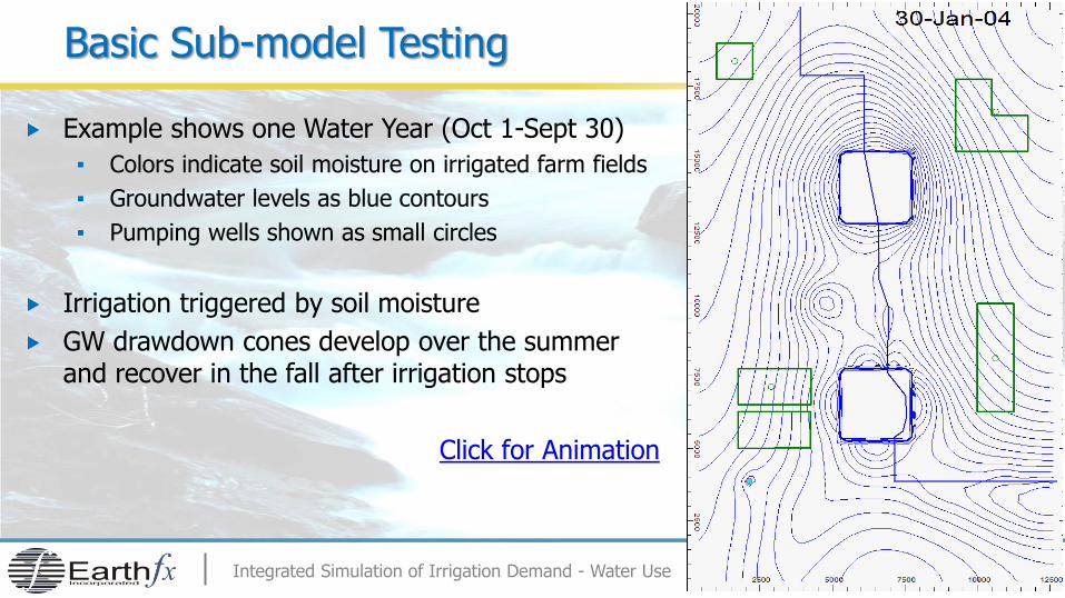
Basic Sub-model Testing

Example shows one Water Year (Oct 1-Sept 30)

▪ Colors indicate soil moisture on irrigated farm fields

▪ Groundwater levels as blue contours

▪ Pumping wells shown as small circles

Irrigation triggered by soil moisture

GW drawdown cones develop over the summer and recover in the fall after irrigation stops

Click for Animation



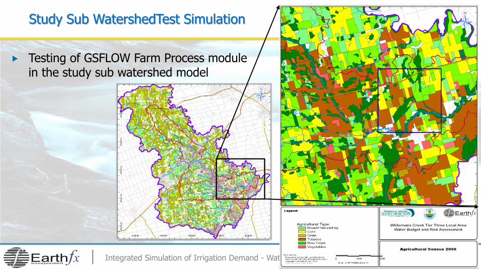
Study Sub WatershedTest Simulation

Testing of GSFLOW Farm Process module in the study sub watershed model


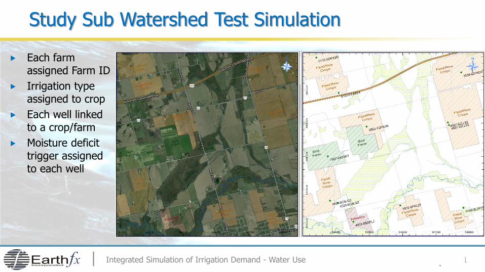
Study Sub Watershed Test Simulation

Each farm assigned Farm ID

Irrigation type assigned to crop

Each well linked to a crop/farm

Moisture deficit trigger assigned to each well


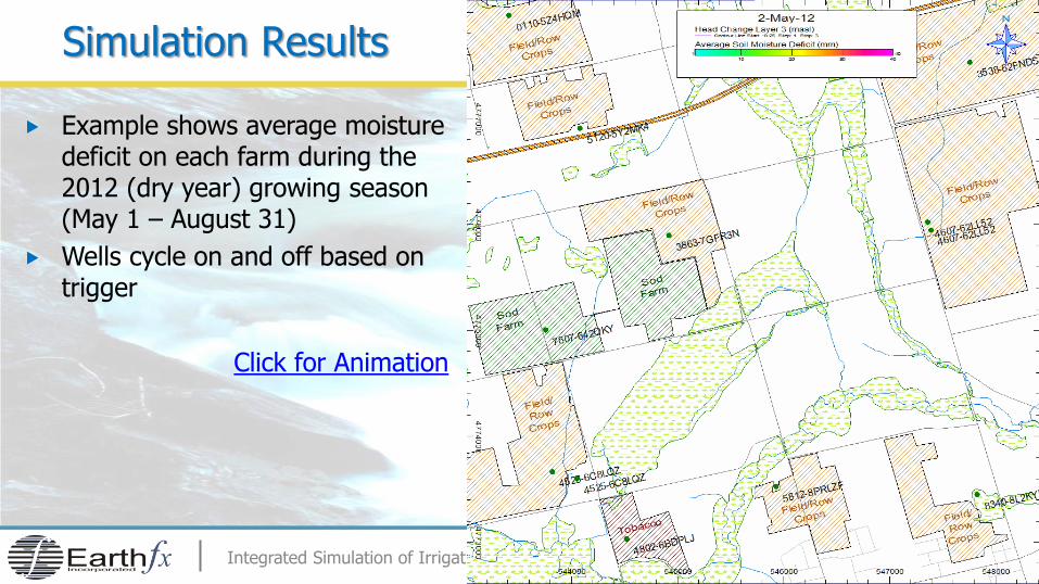
Simulation Results

Example shows average moisture deficit on each farm during the 2012 (dry year) growing season (May 1 – August 31)

Wells cycle on and off based on trigger

Click for Animation



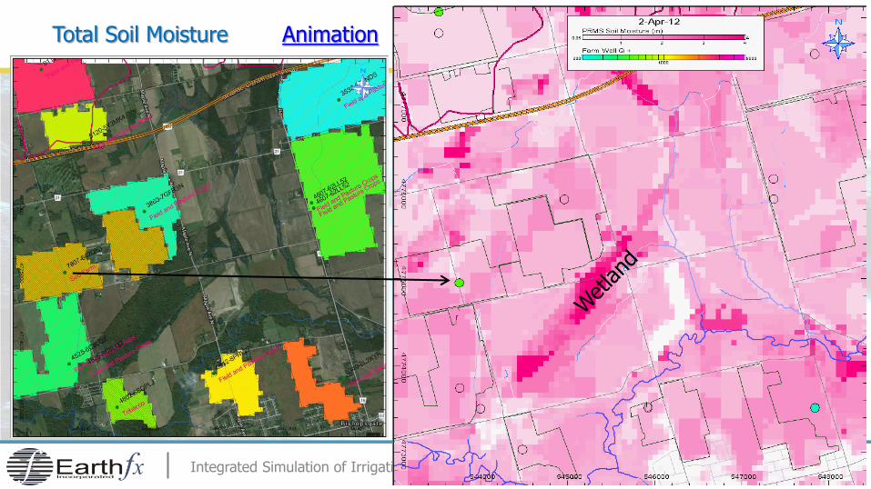
Total Soil Moisture Animation

Example shows



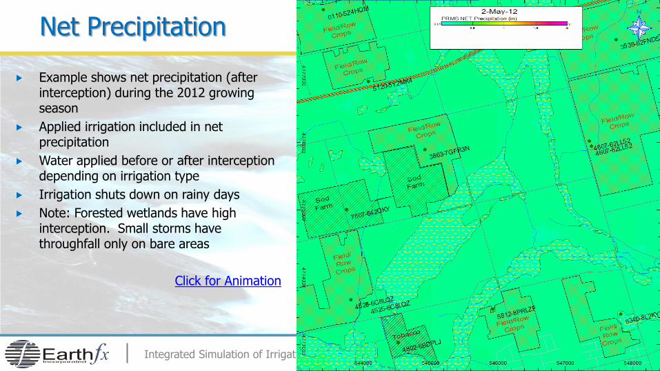
Net Precipitation

Example shows net precipitation (after interception) during the 2012 growing season

Applied irrigation included in net precipitation

Water applied before or after interception depending on irrigation type

Irrigation shuts down on rainy days

Note: Forested wetlands have high interception. Small storms have throughfall only on bare areas

Click for Animation



Whitemans Simulation: Soil Moisture and Pumping

Example compares soil moisture deficit versus trigger in an irrigated field.

Pump comes on when moisture levels drop below target

Example also compares simulated pumping versus reported for the farm.

Simulated irrigation season likely starts too early. Pumps may stay on too long. More calibration needed.


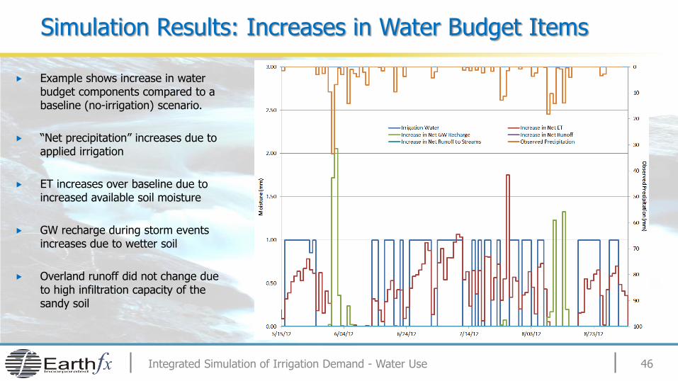
Simulation Results: Increases in Water Budget Items

Example shows increase in water budget components compared to a baseline (no-irrigation) scenario.

“Net precipitation” increases due to applied irrigation

ET increases over baseline due to increased available soil moisture

GW recharge during storm events increases due to wetter soil

Overland runoff did not change due to high infiltration capacity of the sandy soil


47

Conclusions

Integrated Simulation of Irrigation Demand - Conclusions & Next Steps

Predicting and simulating cumulative water use under future drought conditions requires an understanding of farm irrigation processes and triggers

The new GSFLOW irrigation module developed by Earthfx integrates farm water management practices into a comprehensive and fully integrated SW/GW model

Model provides detailed farm water budget

Historic climate and water use data can be used to develop farm-specific water use practices and triggers.

▪ Alternatively, standard or best management practices could be represented in the model to simulate and evaluate improved water use and informed permit renewal

incorporating a dynamic irrigation demand module into an integrated surface water/groundwater model...

Engineering