On the Logical Origin of the Laws Governing the

Fundamental Forces of Nature: A New

Algebraic-Axiomatic Matrix Approach

Ramin Zahedi

To cite this version:

Ramin Zahedi. On the Logical Origin of the Laws Governing the Fun- damental Forces of Nature: A New Algebraic-Axiomatic Matrix Approach. Eprints.Lib.Hokudai.ac.jp/dspace/handle/2115/59279/ , HOKKAIDO UNIVERSITY COL- LECTION OF SCHOLARLY AND ACADEMIC PAPERS., 2015, 16 (1), pp.90.

Distributed under a Creative Commons Attribution - NonCommercial - NoDerivatives 4.0International License

HAL Id: hal-01476703

Submitted on 29 Mar 2017

HAL is a multi-disciplinary open access

archive for the deposit and dissemination of sci-entific research documents, whether they are pub-

lished or not. The documents may come fromteaching and research institutions in France orabroad, or from public or private research centers.

L’archive ouverte pluridisciplinaire HAL, est

destinee au depot et a la diffusion de documentsscientifiques de niveau recherche, publies ou non,

emanant des etablissements d’enseignement et derecherche francais ou etrangers, des laboratoirespublics ou prives.

Instructions for use

Title On the Logical Origin of the Laws Governing the Fundamental Forces of Nature : A New AxiomaticMatrix Approach

Author(s) Zahedi, Ramin

Citation Archive for Studies in Logic (AFSIL), 16(1): 1-87

Issue Date 2015-01

Doc URL http://hdl.handle.net/2115/59279

Right CC Attribution-NonCommercial-NoDerivatives 4.0 International License. License URL:https://creativecommons.org/licenses/by-nc-nd/4.0/

Type article

Note

Acknowledgements: Special thanks are extended to Prof. and Academician Vitaly L. Ginzburg (Russia),Prof. and Academician Dmitry V. Shirkov (Russia), Prof. Leonid A . Shelepin (Russia), Prof. VladimirYa. Fainberg (Russia), Prof. Wolfgang Rindler (USA), Prof. Roman W. Jackiw (USA), Prof. RogerPenrose (UK), Prof. Steven Weinberg (USA), Prof. Ezra T. Newman (USA), Prof. Graham Jameson(UK), Prof. Sergey A. Reshetnjak (Russia), Prof. Sir Michael Atiyah (UK) (who, in particular, kindlyencouraged me to continue this work as a new unorthodox (primary) mathematical approach tofundamental physics), and many others for their support and valuable guidance during my studies andresearch.

Note(URL) https://cds.cern.ch/record/1980381/

File Information R.A.Zahedi--Forces.of.Nature.Laws-Jan.2015-signed.pdf

Hokkaido University Collection of Scholarly and Academic Papers : HUSCAP

1

On the Logical Origin of the Laws Governing the Fundamental Forces of Nature: A New Algebraic-Axiomatic (Matrix) Approach

by: Ramin Zahedi *

Logic and Philosophy of Science Research Group**, Hokkaido University, Japan

28 Jan 2015 The main idea and arguments of this article are based on my earlier publications (Refs. [1]-[4], Springer, 1996-1998). In this article, as a new mathematical approach to origin of the laws of nature, using a new basic algebraic axiomatic (matrix) formalism based on the ring theory and Clifford algebras (presented in Sec.2), “it is shown that certain mathematical forms of fundamental laws of nature, including laws governing the fundamental forces of nature (represented by a set of two definite classes of general covariant massive field equations, with new matrix formalisms), are derived uniquely from only a very few axioms”; where in agreement with the rational Lorentz group, it is also basically assumed that the components of relativistic energy-momentum can only take rational values. In essence, the main scheme of this new mathematical axiomatic approach to fundamental laws of nature is as follows. First based on the assumption of rationality of D-momentum, by linearization (along with a parameterization procedure) of the Lorentz invariant energy-momentum quadratic relation, a unique set of Lorentz invariant systems of homogeneous linear equations (with matrix formalisms compatible with certain Clifford, and symmetric algebras) is derived. Then by first quantization (followed by a basic procedure of minimal coupling to space-time geometry) of these determined systems of linear equations, a set of two classes of general covariant massive (tensor) field equations (with matrix formalisms compatible with certain Clifford, and Weyl algebras) is derived uniquely as well. Each class of the derived general covariant field equations also includes a definite form of torsion field appeared as generator of the corresponding field‘ invariant mass. In addition, it is shown that the (1+3)-dimensional cases of two classes of derived field equations represent a new general covariant massive formalism of bispinor fields of spin-2, and spin-1 particles, respectively. In fact, these uniquely determined bispinor fields represent a unique set of new generalized massive forms of the laws governing the fundamental forces of nature, including the Einstein (gravitational), Maxwell (electromagnetic) and Yang-Mills (nuclear) field equations. Moreover, it is also shown that the (1+2)-dimensional cases of two classes of these field equations represent (asymptotically) a new general covariant massive formalism of bispinor fields of spin-3/2 and spin-1/2 particles, corresponding to the Dirac and Rarita–Schwinger equations. As a particular consequence, it is shown that a certain massive formalism of general relativity – with a definite form of torsion field appeared originally as the generator of gravitational field‘s invariant mass – is obtained only by first quantization (followed by a basic procedure of minimal coupling to space-time geometry) of a certain set of special relativistic algebraic matrix equations. It has been also proved that Lagrangian densities specified for the originally derived new massive forms of the Maxwell, Yang-Mills and Dirac field equations, are also gauge invariant, where the invariant mass of each field is generated solely by the corresponding torsion field. In addition, in agreement with recent astronomical data, a new particular form of massive boson is identified (corresponding to the U(1) gauge symmetry group) with invariant mass: mγ ≈ 4.90571×10-50 kg, generated by a coupled torsion field of the background space-time geometry. Moreover, based on the definite mathematical formalism of this axiomatic approach, along with the C, P and T symmetries (represented basically by the corresponding quantum operators) of the fundamentally derived field equations, it is concluded that the universe could be realized solely with the (1+2) and (1+3)-dimensional space-times (where this conclusion, in particular, is based on the T-symmetry). It is proved that 'CPT' is the only (unique) combination of C, P, and T symmetries that could be defined as a symmetry for interacting fields. In addition, on the basis of these discrete symmetries of derived field equations, it has been also shown that only left-handed particle fields (along with their complementary right-handed fields) could be coupled to the corresponding (any) source currents. Furthermore, it has been shown that the metric of background space-time is diagonalized for the uniquely derived fermion field equations (defined and expressed solely in (1+2)-dimensional space-time), where this property generates a certain set of additional symmetries corresponding uniquely to the SU(2)LU(2)R symmetry group for spin-1/2 fermion fields (representing ―1+3‖ generations of four fermions, including a group of eight leptons and a group of eight quarks), and also the SU(2)LU(2)R and SU(3) gauge symmetry groups for spin-1 boson fields coupled to the spin-1/2 fermionic source currents. Hence, along with the known elementary particles, eight new elementary particles, including four new charge-less right-handed spin-1/2 fermions (two leptons and two quarks), a spin-3/2 fermion, and also three new spin-1 (massive) bosons, are predicted uniquely by this mathematical axiomatic approach. As a particular result, based on the definite formulation of derived Maxwell (and Yang-Mills) field equations, it has been also concluded that magnetic monopoles could not exist in nature.1

1. Introduction and Summary Why do the fundamental forces of nature (i.e., the forces that appear to cause all the movements and

interactions in the universe) manifest in the way, shape, and form that they do? This is one of the

greatest ontological questions that science can investigate. In this article, we‘ll consider this basic and

* Email: zahedi@let.hokudai.ac.jp, zahedi.r@gmail.com . **(This work has been done and published during my research fellowship, 2007–2016). 1. https://indico.CERN.ch/event/344173/contribution/1740565/attachments/1140145/1646101/R.A.Zahedi--Forces.of.Nature.Laws-Jan.2015-signed.pdf ,

https://eprints.lib.Hokudai.ac.jp/dspace/handle/2115/59279, https://cds.CERN.ch/record/1980381, https://hal-Paris1.archives-ouvertes.fr/hal-01476703, https://ui.adsabs.harvard.edu/#abs/2015arXiv150101373Z, https://Dumas.CCSD.CNRS.fr/TDS-MACS/hal-01476703, https://InspireHep.net/record/1387680 Copyright: CC Attribution-NonCommercial-NoDerivatives 4.0 International License. License URL: https://creommons.org/licenses/by-nc-nd/4.0/

2017

Jun

15

[phy

sics

.gen

-ph]

ar

Xiv

:150

1.01

373v

16

2

and crucial question (and a number of relevant issues) via a new axiomatic mathematical formalism.

By definition, a basic law of physics (or a scientific law in general) is: ―A theoretical principle

deduced from particular facts, applicable to a defined group or class of phenomena, and expressible

by the statement that a particular phenomenon always occurs if certain conditions be present‖ [55].

Eugene Wigner's foundational paper, ―On the Unreasonable Effectiveness of Mathematics in the

Natural Sciences‖, famously observed that purely mathematical structures and formalisms often lead

to deep physical insights, in turn serving as the basis of highly successful physical theories [50].

However, all the known fundamental laws of physics (and corresponding mathematical formalisms

which are used for their representations), are generally the conclusions of a number of repeated

experiments and observations over years and have become accepted universally within the scientific

communities [56, 57].

This article is based on my earlier publications (Refs. [1]–[4], Springer, 1996-1998). In this article, as

a new mathematical approach to origin of the laws of nature, using a new basic algebraic axiomatic

(matrix) formalism based on the ring theory and Clifford algebras (presented in Sec.2), “it is shown

that certain mathematical forms of fundamental laws of nature, including laws governing the

fundamental forces of nature (represented by a set of two definite classes of general covariant

massive field equations, with new matrix formalisms), are derived uniquely from only a very few

axioms”; where in agreement with the rational Lorentz group, it is also basically assumed that the

components of relativistic energy-momentum can only take rational values.. Concerning the basic

assumption of rationality of relativistic energy-momentum, it is necessary to note that the rational

Lorentz symmetry group is not only dense in the general form of Lorentz group, but also is

compatible with the necessary conditions required basically for the formalism of a consistent

relativistic quantum theory [77]. In essence, the main scheme of this new mathematical axiomatic

approach to fundamental laws of nature is as follows. First based on the assumption of rationality of

D-momentum, by linearization (along with a parameterization procedure) of the Lorentz invariant

energy-momentum quadratic relation, a unique set of Lorentz invariant systems of homogeneous

linear equations (with matrix formalisms compatible with certain Clifford, and symmetric algebras)

is derived. Then by first quantization (followed by a basic procedure of minimal coupling to space-

time geometry) of these determined systems of linear equations, a set of two classes of general

covariant massive (tensor) field equations (with matrix formalisms compatible with certain Clifford,

and Weyl algebras) is derived uniquely as well. Each class of the derived general covariant field

equations also includes a definite form of torsion field appeared as generator of the corresponding

field‘ invariant mass. In addition, it is shown that the (1+3)-dimensional cases of two classes of

derived field equations represent a new general covariant massive formalism of bispinor fields of

spin-2, and spin-1 particles, respectively. In fact, these uniquely determined bispinor fields represent

a unique set of new generalized massive forms of the laws governing the fundamental forces of

nature, including the Einstein (gravitational), Maxwell (electromagnetic) and Yang-Mills (nuclear)

field equations. Moreover, it is also shown that the (1+2)-dimensional cases of two classes of these

field equations represent (asymptotically) a new general covariant massive formalism of bispinor

fields of spin-3/2 and spin-1/2 particles, respectively, corresponding to the Dirac and Rarita–

Schwinger equations.

3

As a particular consequence, it is shown that a certain massive formalism of general relativity – with

a definite form of torsion field appeared originally as the generator of gravitational field‘s invariant

mass – is obtained only by first quantization (followed by a basic procedure of minimal coupling to

space-time geometry) of a certain set of special relativistic algebraic matrix equations. It has been

also proved that Lagrangian densities specified for the originally derived new massive forms of the

Maxwell, Yang-Mills and Dirac field equations, are also gauge invariant, where the invariant mass of

each field is generated solely by the corresponding torsion field. In addition, in agreement with recent

astronomical data, a new particular form of massive boson is identified (corresponding to U(1) gauge

group) with invariant mass: mγ ≈ 4.90571×10-50kg, generated by a coupled torsion field of the

background space-time geometry.

Moreover, based on the definite mathematical formalism of this axiomatic approach, along with

the C, P and T symmetries (represented basically by the corresponding quantum operators) of the

fundamentally derived field equations, it has been concluded that the universe could be realized

solely with the (1+2) and (1+3)-dimensional space-times (where this conclusion, in particular, is

based on the T-symmetry). It is proved that 'CPT' is the only (unique) combination of C, P, and T

symmetries that could be defined as a symmetry for interacting fields. In addition, on the basis of

these discrete symmetries of derived field equations, it has been also shown that only left-handed

particle fields (along with their complementary right-handed fields) could be coupled to the

corresponding (any) source currents. Furthermore, it has been shown that the metric of background

space-time is diagonalized for the uniquely derived fermion field equations (defined and expressed

solely in (1+2)-dimensional space-time), where this property generates a certain set of additional

symmetries corresponding uniquely to the SU(2)LU(2)R symmetry group for spin-1/2 fermion fields

(representing ―1+3‖ generations of four fermions, including a group of eight leptons and a group of

eight quarks), and also the SU(2)LU(2)R and SU(3) gauge symmetry groups for spin-1 boson fields

coupled to the spin-1/2 fermionic source currents. Hence, along with the known elementary particles,

eight new elementary particles, including: four new charge-less right-handed spin-1/2 fermions (two

leptons and two quarks, represented by ―ze , zn and zu , zd‖), a spin-3/2 fermion, and also three new

spin-1 massive bosons (represented by ",~

,~

" ZWW

, where in particular, the new boson Z

is

complementary right-handed particle of ordinary Z boson), have been predicted uniquely and

expressly by this new mathematical axiomatic approach.

As a particular result, in Sec. 3-4-2, based on the definite and unique formulation of the derived

Maxwell‘s equations (and also determined Yang-Mills equations, represented uniquely with two

specific forms of gauge symmetries, in 3-6-3-2), it has been also concluded generally that magnetic

monopoles could not exist in nature.

4

1-1. The main results obtained in this article are based on the following three basic assumptions

(as postulates):

(1)- “A new definite axiomatic generalization of the axiom of ―no zero divisors‖ of integral

domains (including the ring of integers ℤ);” This algebraic postulate (as a new mathematical concept) is formulated as follows:

“Let ][ ijaA be a nn matrix with entries expressed by the following linear homogeneous

polynomials in s variables over the integral domain ℤ: ;),...,,,(1

321

s

k

kijksijij bHbbbbaa suppose

also ― r ℕ: ns IbbbbF Ar ),...,,,( 321 ‖, where ),...,,,( 321 sbbbbF is a homogeneous polynomial of

degree r ≥ 2, and nI is nn identity matrix. Then the following axiom is assumed (as a new

axiomatic generalization of the ordinary axiom of ―no zero divisors‖ of integral domain ℤ):

)0,0()0( MMAAr (1)

where M is a non-zero arbitrary 1n column matrix”.

The axiomatic relation (1) is a logical biconditional, where )0( rA and )0,0( MMA are

respectively the antecedent and consequent of this biconditional. In addition, based on the initial

assumption r ℕ: ns IbbbbF Ar ),...,,,( 321 , the axiomatic biconditional (1) could be also

represented as follows:

)0,0(]0),...,,,([ 321 MMAbbbbF s (1-1)

where the homogeneous equation 0),...,,,( 321 sbbbbF , and system of linear equations

)0,0( MMA are respectively the antecedent and consequent of biconditional (1-1). The

axiomatic biconditional (1-1), defines a system of linear equations of the type 0MA )0( M ,

as the algebraic equivalent representation of thr degree homogeneous equation 0),...,,,( 321 sbbbbF

(over the integral domain ℤ). In addition, according to the Ref. [6], since 0),...,,,( 321 sbbbbF is a

homogeneous equation over ℤ, it is also concluded that homogeneous equations defined over the

field of rational numbers ℚ,

obey the axiomatic relations (1) and (1-1) as well. As particular outcome

of this new mathematical axiomatic formalism (based on the axiomatic relations (1) and (1-1),

including their basic algebraic properties), in Sec. 3-4, it is shown that using, a unique set of general

covariant massive (tensor) field equations (with new matrix formalism compatible with Clifford, and

Weyl algebras), corresponding to the fundamental field equations of physics, are derived – where, in

agreement with the rational Lorentz symmetry group, it has been basically assumed that the

components of relativistic energy-momentum can only take the rational values. In Sections 3-2 – 3-6,

we present in detail the main applications of this basic algebraic assumption (along with the

following basic assumptions (2) and (3)) in fundamental physics.

5

(2)- “In agreement with the rational Lorentz symmetry group, we assume basically that the

components of relativistic energy-momentum (D-momentum) can only take the rational values;” Concerning this assumption, it is necessary to note that the rational Lorentz symmetry group is not

only dense in the general form of Lorentz group, but also is compatible with the necessary conditions

required basically for the formalism of a consistent relativistic quantum theory [77]. Moreover, this

assumption is clearly also compatible with any quantum circumstance in which the energy-

momentum of a relativistic particle is transferred as integer multiples of the quantum of action ―h‖

(Planck constant).

Before defining the next basic assumption, it should be noted that from the basic assumptions (1) and

(2), it follows directly that the Lorentz invariant energy-momentum quadratic relation (represented by

formula (52), in Sec. 3-1-1) is a particular form of homogeneous quadratic equation (represented by

formula (18-2) in Sec. 2-2). Hence, using the set of systems of linear equations that are determined

uniquely as equivalent algebraic representations of the corresponding set of quadratic homogeneous

equations (given by equation (18-2) in various number of unknown variables, respectively), a unique set

of the Lorentz invariant systems of homogeneous linear equations (with matrix formalisms compatible

with certain Clifford, and symmetric algebras) are also determined, representing equivalent algebraic

forms of the energy-momentum quadratic relation in various space-time dimensions, respectively.

Subsequently, we‘ve shown that by first quantization (followed by a basic procedure of minimal

coupling to space-time geometry) of these determined systems of linear equations, a unique set of

two definite classes of general covariant massive (tensor) field equations (with matrix formalisms

compatible with certain Clifford, and Weyl algebras) is also derived, corresponding to various space-

time dimensions, respectively. In addition, it is also shown that this derived set of two classes of general

covariant field equations represent new tensor massive (matrix) formalism of the fundamental field

equations of physics, corresponding to fundamental laws of nature (including the laws governing the

fundamental forces of nature). Following these essential results, in addition to the basic assumptions (1)

and (2), it would be also basically assumed that:

(3)- “We assume that the mathematical formalism of the fundamental laws of nature, are

defined solely by the axiomatic matrix constitution formulated uniquely on the basis of

postulates (1) and (2)”.

In addition to this basic assumption, in Sec. 3-5, the C, P and T symmetries of the uniquely derived

general covariant field equations (that are field equations (3) and (4) in Sec. 1-2-1), would be represented

basically by their corresponding quantum matrix operators.

1-2. In the following, we present a summary description of the main consequences of basic

assumptions (1) – (3) (mentioned in Sec. 1-1) in fundamental physics. In this article, the metric

signature (+ − ... −), the geometrized units [9] and also the following sign conventions have been

used in the representations of the Riemann curvature tensor R , Ricci tensor R and Einstein

tensor G :

....8,),()(

GRRRR (2)

6

1-2-1. On the basis of assumptions (1) – (3), two sets of the general covariant field equations

(compatible with the Clifford algebras) are derived solely as follows:

0)~( )(

0 R

R kmi

(3)

0)~( )(

0 F

F kmDi

(4)

where

~, (5)

i and Di are the general relativistic forms of energy-momentum quantum operator (where

is the general covariant derivative and D is gauge covariant derivative, defining in Sections 3-

4, 3-4-1 and 3-4-2), )(

0

Rm and )(

0

Fm are the fields‘ invariant masses, )0,...,0,( 00gck is the general

covariant velocity in stationary reference frame (that is a time-like covariant vector), and are

two contravariant square matrices (given by formulas (6) and (7)), R is a column matrix given by

formulas (6) and (7), which contains the components of field strength tensor R (equivalent to the

Riemann curvature tensor), and also the components of a covariant quantity which defines the

corresponding source current (by relations (6) and (7)), F is also a column matrix given by

formulas (6) and (7), which contains the components of tensor field F (defined as the gauge field

strength tensor), and also the components of a covariant quantity which defines the corresponding

source current (by relations (6) and (7)). In Sec. 3-5, based on a basic class of discrete symmetries of

general covariant field equations (3) and (4), it would be concluded that these equations could be

defined solely in (1+2) and (1+3) space-time dimensions, where the (1+2) and (1+3)-dimensional

cases these field equations are given uniquely as follows (in terms of the above mentioned

quantities), respectively:

- For (1+2)-dimensional space-time we have:

,0

0,

0

0,

00

0,

)(0

003

3

12

2

1

10

010

0

,01

00,

00

10,

10

00,

00

01,

0

0,

0

0 3210

1

0

20

1

2

;)(

,)(,

0,

0

)()(

0)(

)()(

0)(

)(

21

10

)(

21

10

FF

F

RR

R

F

F

R

R

kim

DJ

kim

J

F

F

R

R

(6)

- For (1+3)-dimensional space-time of we get:

,0

0,

0

0,

00

0)(,

)(0

002

3

13

2

1

10

010

0

7

,0

0,

0

0,

0

0,

0

06

7

37

6

3

4

5

25

4

2

,

0000

0010

0100

0000

,

0001

0000

0000

1000

,

1000

0100

0000

0000

,

0000

0000

0010

0001

3210

,

0000

0000

0001

0010

,

0100

1000

0000

0000

,

0000

0001

0000

0100

,

0010

0000

1000

0000

7654

;)(

,)(,

0,

0

)()(

0)(

)()(

0)(

)(

12

31

23

30

20

10

)(

12

31

23

30

20

10

FF

F

RR

R

F

F

R

R

kim

DJ

kim

J

F

F

F

F

F

F

R

R

R

R

R

R

(7)

In formulas (6) and (7), )(RJ and )(FJ are the covariant source currents expressed necessarily in

terms of the covariant quantities

)(R

and )(F (as initially given quantities). Moreover, in Sections

3-4 – 3-6, it has been also shown that the field equations in (1+2) dimensions, are compatible with

the matrix representation of Clifford algebra Cℓ1,2, and represent (asymptotically) new general

covariant massive formalism of bispinor fields of spin-3/2 and spin-1/2 particles, respectively. It has

been also shown that these field equations in (1+3) dimensions are compatible with the matrix

representation of Clifford algebra Cℓ1,3, and represent solely new general covariant massive

formalism of bispinor fields of spin-2 and spin-1 particles, respectively.

1-2-2. In addition, from the field equations (3) and (4), the following field equations (with ordinary

tensor formulations) could be also obtained, respectively:

,

RTRTRTRRR

(3-1)

)()(

0 )( RR JRkimR

; (3-2)

),()(

R

)()(

0)( )( RR

R kim

J

, ).(

2

)(

0 kgkg

imT

R

(3-3)

8

and

,0 FDFDFD

(4-1)

)(FJFD

; (4-2)

ADADF

,

)()(

0)( )( FF

F kim

DJ

, ).(

2

)(

0 kgkg

imZ

F

(4-3)

where in equations (3-1) – (3-2), is the affine connection given by:

K ,

is

the Christoffel symbol (or the torsion-free connection), K is a contorsion tensor defined by:

kgimK R )2( )(

0 (that is anti-symmetric in the first and last indices), T is its corresponding

torsion tensor given by: KKT (as the generator of the gravitational field‘s invariant mass),

is general covariant derivative defined with torsion T . In equations (4-1) – (4-3), D

is the

general relativistic form of gauge covariant derivative defined with torsion field Z (which generates

the gauge field‘s invariant mass), and A denotes the corresponding gauge (potential) field.

1-2-3. In Sec. 3-5, on the basis of definite mathematical formalism of this axiomatic approach,

along with the C, P and T symmetries (represented basically by the corresponding quantum

operators, in Sec. 3-5) of the fundamentally derived field equations, it has been concluded that the

universe could be realized solely with the (1+2) and (1+3)-dimensional space-times (where this

conclusion, in particular, is based on the T-symmetry). It is proved that 'CPT' is the only (unique)

combination of C, P, and T symmetries that could be defined as a symmetry for interacting fields. In

addition, on the basis of these discrete symmetries of derived field equations, it has been also shown

that only left-handed particle fields (along with their complementary right-handed fields) could be

coupled to the corresponding (any) source currents. Furthermore, it has been shown that the metric of

background space-time is diagonalized for the uniquely derived fermion field equations (defined and

expressed solely in (1+2)-dimensional space-time), where this property generates a certain set of

additional symmetries corresponding uniquely to the SU(2)LU(2)R symmetry group for spin-1/2

fermion fields (representing ―1+3‖ generations of four fermions, including a group of eight leptons

and a group of eight quarks), and also the SU(2)LU(2)R and SU(3) gauge symmetry groups for spin-

1 boson fields coupled to the spin-1/2 fermionic source currents. Hence, along with the known

elementary particles, eight new elementary particles, including: four new charge-less right-handed

spin-1/2 fermions (two leptons and two quarks, represented by ―ze , zn and zu , zd‖), a spin-3/2

fermion, and also three new spin-1 massive bosons (represented by ",~

,~

" ZWW

, where in

particular, the new boson Z

is complementary right-handed particle of ordinary Z boson), have

been predicted uniquely by this new mathematical axiomatic approach (as shown in Sections 3-6-1-2

and 3-6-3-2).

1-2-4. As a particular consequence, in Sec. 3-4-2, it is shown that a certain massive formalism of

the general theory of relativity – with a definite torsion field which generates the gravitational field‗s

mass – is obtained only by first quantization (followed by a basic procedure of minimal coupling to

space-time geometry) of a set of special relativistic algebraic matrix relations. In Sec. 3-4-4, it is also

proved that Lagrangian densities specified for the derived unique massive forms of Maxwell, Yang-

9

Mills and Dirac equations, are gauge invariant as well, where the invariant mass of each field is

generated by the corresponding torsion field. In addition, in Sec. 3-4-5, in agreement with recent

astronomical data, a new massive boson is identified (corresponding to U(1) gauge group) with

invariant mass: mγ ≈ 4.90571×10-50kg, generated by a coupling torsion field of the background

space-time geometry. Furthermore, in Sec. 3-4-2, based on the definite and unique formulation of the

derived Maxwell‗s equations (and also determined Yang-Mills equations, represented unqiely with

two specific forms of gauge symmetries), it is also concluded that magnetic monopoles could not

exist in nature.

1-2-5. As it would be also shown in Sec. 3-4-3, if the Ricci curvature tensor R is defined basically

by the following relation in terms of Riemann curvature tensor (which is determined by field

equations (3-1) – (3-3)):

Rkim

Rkim

Rkim RRR

)()()()(

0

)(

0

)(

0

, (8-1)

then from this expression for the current in terms of the stress-energy tensor T :

])()[(8])()[(8)(

0

)(

0

)(

0

)(

0)(

Tgkim

Tgkim

BTkim

Tkim

JRRRR

R

(8-2)

where TT , the gravitational field equations (including a cosmological constant emerged

naturally in the course of derivation process) could be equivalently derived particularly from the

massless case of tensor field equations (3-1) – (3-3) in (1+3) space-time dimensions, as follows:

gTgTR 48 (9)

1-2-6. Let we emphasize again that the results obtained in this article, are direct outcomes of a new

algebraic-axiomatic approach1 which has been presented in Sec. 2. This algebraic approach, in the

form of a basic linearization theory, has been constructed on the basis of a new single axiom (that is

the axiom (17) in Sec. 2-1) proposed to replace with the ordinary axiom of ―no zero divisors‖ of

integral domains (that is the axiom (16) in Sec. 2). In fact, as noted in Sec. 1-1 and also Sec. 2-1, the

new proposed axiom is a definite generalized form of ordinary axiom (16), which particularly has

been formulated in terms of square matrices (using basically as primary objects for representing the

elements of underlying algebra, i.e. integral domains including the ring of integers). In Sec. 3, based

on this new algebraic axiomatic formalism, as a new mathematical approach to origin of the laws of

nature, “it is shown that certain mathematical forms of fundamental laws of nature, including laws

governing the fundamental forces of nature (represented by a set of two definite classes of general

covariant massive field equations, with new matrix formalisms), are derived uniquely from only a

very few axioms”; where in agreement with the rational Lorentz group, it is also basically assumed

that the components of relativistic energy-momentum can only take rational values.

--------------------------------------------------------------------------------------------------------- 1.

Besides, we may argue that our presented axiomatic matrix approach (for a direct derivation and formulating the fundamental laws of nature

uniquely) is not subject to the Gödel's incompleteness theorems [51]. As in our axiomatic approach, firstly, we've basically changed (i.e.

replaced and generalized) one of the main Peano axioms (when these axioms algebraically are augmented with the operations of addition and multiplication [52, 53, 54]) for integers, which is the algebraic axiom of ―no zero divisors‖.

Secondly, based on our approach, one of the axiomatic properties of integers (i.e. axiom of ―no zero divisors‖) could be accomplished solely

by the arbitrary square matrices (with integer components). This axiomatic reformulation of algebraic properties of integers thoroughly has been presented in Sec. 2 of this article.

10

2. Theory of Linearization: a New Algebraic-Axiomatic (Matrix) Approach

Based on the Ring Theory

In this Section a new algebraic theory of linearization (including the simultaneous parameterization) of

the homogeneous equations has been presented that is formulated on the basis of ring theory and matrix

representation of the generalized Clifford algebras (associated with homogeneous forms of degree r ≥ 2

defined over the integral domain ℤ).

Mathematical models of physical processes include certain classes of mathematical objects and relations

between these objects. The models of this type, which are most commonly used, are groups, rings, vector

spaces, and linear algebras. A group is a set G with a single operation (multiplication) cba ;

Gcba ,, which obeys the known conditions [5]. A ring is a set of elements R, where two binary

operations, namely, addition and multiplication, are defined. With respect to addition this set is a group,

and multiplication is connected with addition by the distributivity laws: ),()()( cabacba

)()()( acabacb ; Rcba ,, . The rings reflect the structural properties of the set R. As

distinct from the group models, those connected with rings are not frequently applied, although in physics

various algebras of matrices, algebras of hyper-complex numbers, Grassman and Clifford algebras are

widely used. This is due to the intricacy of finding a connection between the binary relations of addition

and multiplication and the element of the rings [5, 2]. This Section is devoted to the development of a

rather simple approach of establishing such a connection and an analysis of concrete problems on this

basis.

I‘ve found out that if the algebraic axiom of ―no zero divisors‖ of integral domains is generalized

expressing in terms of the square matrices (as it has been formulated by the axiomatic relation (17)),

fruitful new results hold. In this Section, first on the basis of the matrix representation of the generalized

Clifford algebras (associated with homogeneous polynomials of degree r ≥ 2 over the integral domain ℤ),

we‘ve presented a new generalized formulation of the algebraic axiom of ―no zero divisors‖ of integral

domains. Subsequently, a linearization theory has been constructed axiomatically that implies (necessarily

and sufficiently) any homogeneous equation of degree r ≥ 2 over the integral domain ℤ, should be

linearized (and parameterized simultaneously), and then its solution be investigated systematically via its

equivalent linearized-parameterized formolation (representing as a certain type of system of linear

homogeneous equations). In Sections 2-2 and 2-4, by this axiomatic approach a class of homogeneous

quadratic equations (in various numbers of variables) over ℤ has been considered explicitly

2-1. The basic properties of the integral domain ℤ with binary operations ),( are represented as

follows, respectively [5] ( aaa kji ,...,, ℤ):

- Closure: lk aa ℤ , lk aa ℤ (10)

- Associativity: ,)()( plkplk aaaaaa plkplk aaaaaa )()( (11)

- Commutativity: ,kllk aaaa kllk aaaa (12)

- Existence of identity elements:

,0 kk aa kk aa 1 (13)

- Existence of inverse element (for operator of addition):

0)( kk aa (14)

11

- Distributivity: ),()()( pklkplk aaaaaaa )()()( plpkplk aaaaaaa (15)

- No zero divisors (as a logical bi-conditional for operator of multiplication):

)0,0(0 llkk aaaa (16)

Axiom (16), equivalently, could be also expressed as follows,

0)00( lklk aaaa (16-1)

In this article as a new basic algebraic property of the domain of integers, we present the following

new axiomatic generalization of the ordinary axiom of ―no zero divisors‖ (16), which particularly has

been formulated on the basis of matrix formalism of Clifford algebras (associated with homogeneous

polynomials of degree r ≥ 2, over the integral domain ℤ):

“Let ][ ijaA be a nn matrix with entries expressed by the following linear homogeneous

polynomials in s variables over the integral domain ℤ: ;),...,,,(1

321

s

k

kijksijij bHbbbbaa suppose

also ― r ℕ: ns IbbbbF Ar ),...,,,( 321 ‖, where ),...,,,( 321 sbbbbF is a homogeneous polynomial of

degree r ≥ 2, and nI is nn identity matrix. Then the following axiom is assumed (as a new

axiomatic generalization of the ordinary axiom of ―no zero divisors‖ of integral domain ℤ):

)0,0()0( MMAAr (17)

where M is a non-zero arbitrary 1n column matrix”.

The axiomatic relation (17) is a logical biconditional, where )0( rA and )0,0( MMA are

respectively the antecedent and consequent of this biconditional. In addition, based on the initial

assumption r ℕ: ns IbbbbF Ar ),...,,,( 321 , the axiomatic biconditional (17) could be also

represented as follows:

)0,0(]0),...,,,([ 321 MMAbbbbF s (17-1)

where the homogeneous equation 0),...,,,( 321 sbbbbF , and system of linear equations

)0,0( MMA are respectively the antecedent and consequent of biconditional (17-1). The

axiomatic biconditional (17-1), defines a system of linear equations of the type 0MA )0( M ,

as the algebraic equivalent representation of thr degree homogeneous equation 0),...,,,( 321 sbbbbF

(over the integral domain ℤ). The axiom (17) (or (17-1)) for 1n , is equivalent to the ordinary

axiom of ―no zero divisors‖ (16). In fact, the axiom (16), as a particular case, can be obtained from

the axiom (17) (or (17-1), but not vice versa.

Moreover, according to the Ref. [6], since 0),...,,,( 321 sbbbbF is a homogeneous equation over ℤ, it

is also concluded that homogeneous equations defined over the field of rational numbers ℚ,

obey the

axiomatic relations (17) and (17-1) as well.

12

As a crucial additional issue concerning the axiom (17), it should be noted that the condition

― r ℕ: ns IbbbbF Ar ),...,,,( 321 ‖ which is assumed initially in the axiom (17), is also compatible

with matrix representation of the generalized Clifford algebras [Refs. 40 – 47] associated with the

rth

degree homogeneous polynomials ),...,,,( 321 sbbbbF . In fact, we may represent uniquely the square

matrix A (with assumed properties in the axiom (17)) by this homogeneous linear form:

s

k

kk EbA1

, then the relation: ns IbbbbF Ar ),...,,,( 321 implies that the square matrices kE (which

their entries are independent from the variables kb ) would be generators of the corresponding

generalized Clifford algebra associated with the rth

degree homogeneous polynomial

),...,,,( 321 sbbbbF . However, in some particular cases and applications, we may also assume some

additional conditions for the generators kE , such as the Hermiticity or anti-Hermiticity (see Sections

2-2, 2-4 and 3-1). In Sec. 3, we use these algebraic properties of the square matrix A (corresponding

with the homogeneous quadratic equations), where we present explicitly the main applications of the

axiomatic relations (17) and (17-1) in foundations of physics (where we also use the basic

assumptions (2) and (3) mentioned in Sec. 1-1).

It is noteworthy that since the axiom (17) has been formulated solely in terms of square matrices, in

Ref. [76] we have shown that all the ordinary algebraic axioms (10) – (15) of integral domain ℤ

(except the axiom of ―no zero divisors‖ (16)), in addition to the new axiom (17), could be also

reformulated uniformly in terms of the set of square matrices. Hence, we may conclude that the

square matrices, logically, are the most elemental algebraic objects for representing the basic

properties of set of integers (as the most fundamental set of mathematics).

In the following, based on the axiomatic relation (17-1), we‘ve constructed a corresponding basic

algebraic linearization (including a parameterization procedure) approach applicable to the all classes

of homogeneous equation. Hence, it could be also shown that for any given homogeneous equation

of degree r ≥ 2 over the ring ℤ (or field ℚ), a square matrix A exists that obeys the relation (17-1).

In this regard, for various classes of homogeneous equations, their equivalent systems of linear

equations would be derived systematically.

As a particular crucial case, in Sections 2-2 and 2-4, by

derivation of the systems of linear equations equivalent to a class of quadratic homogeneous

equations (in various number of unknown variables) over the integral domain ℤ (or field ℚ), these

equations have been analyzed (and solved) thoroughly by this axiomatic approach.

In the following,

the basic schemes of this axiomatic linearization-parameterization approach are described.

First, it should be noted that since the entries ija of square matrix A are linear homogeneous forms

expressed in terms of the integral variables pb , i.e.

s

k

kijkij bHa1

, we may also represent the square

matrix A by this linear matrix form:

s

k

kk EbA1

, then (as noted above) the relation:

ns IbbbbF Ar ),...,,,( 321 implies that the square matrices kE (which their entries are independent

from the variables kb ) would be generators of the corresponding generalized Clifford algebra

13

associated with the rth

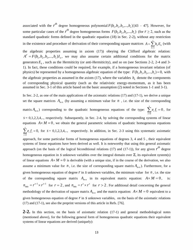
degree homogeneous polynomial ),...,,,( 321 sbbbbF [43 – 47]. However, for

some particular cases of the rth

degree homogeneous forms ),...,,,( 321 sbbbbF (for r ≥ 2, such as the

standard quadratic forms defined in the quadratic equation (18) in Sec. 2-2), without any restriction

in the existence and procedure of derivation of their corresponding square matrices

s

k

kk EbA1

(with

the algebraic properties assuming in axiom (17)) obeying the Clifford algebraic relation:

ns IbbbbF Ar ),...,,,( 321 , we may also assume certain additional conditions for the matrix

generators kE , such as the Hermiticity (or anti-Hermiticity), and so on (see Sections 2-2, 2-4 and 3-

1). In fact, these conditions could be required, for example, if a homogeneous invariant relation (of

physics) be represented by a homogeneous algebraic equation of the type: ,0),...,,,( 321 sbbbbF with

the algebraic properties as assumed in the axiom (17), where the variables kb denote the components

of corresponding physical quantity (such as the relativistic energy-momentum, as it has been

assumed in Sec. 3-1 of this article based on the basic assumption (2) noted in Sections 1-1 and 3-1).

In Sec. 2-2, as one of the main applications of the axiomatic relations (17) and (17-1), we derive a unique

set the square matrices nnA (by assuming a minimum value for n , i.e. the size of the corresponding

matrix nnA ) corresponding to the quadratic homogeneous equations of the type: 00

s

i

ii fe , for

s = 0,1,2,3,4,.., respectively. Subsequently, in Sec. 2-4, by solving the corresponding systems of linear

equations 0MA , we obtain the general parametric solutions of quadratic homogeneous equations

,00

s

i

ii fe for s = 0,1,2,3,4,.., respectively. In addition, in Sec. 2-3 using this systematic axiomatic

approach, for some particular forms of homogeneous equations of degrees 3, 4 and 5 , their equivalent

systems of linear equations have been derived as well. It is noteworthy that using this general axiomatic

approach (on the basis of the logical biconditional relations (17) and (17-1)), for any given rth

degree

homogeneous equation in s unknown variables over the integral domain over ℤ, its equivalent system(s)

of linear equations 0MA is derivable (with a unique size, if in the course of the derivation, we also

assume a minimum value for n , i.e. the size of corresponding square matrix nnA ). Furthermore, for a

given homogeneous equation of degree r in s unknown variables, the minimum value for n , i.e. the size

of the corresponding square matrix nnA in its equivalent matrix equation: 0MA , is:

11

min

ss rrn for 2r , and ss rrn min for 2r . For additional detail concerning the general

methodology of the derivation of square matrix nnA and the matrix equation: 0MA equivalent to a

given homogeneous equation of degree r in s unknown variables, on the basis of the axiomatic relations

(17) and (17-1), see also the preprint versions of this article in Refs. [76].

2-2. In this section, on the basis of axiomatic relation (17-1) and general methodological notes

(mentioned above), for the following general form of homogeneous quadratic equations their equivalent

systems of linear equations are derived (uniquely):

14

0),,...,,,,(

0

1100

s

i

iiss fefefefeQ

(18)

Equation (18) for s = 0,1,2,3,4,.. is represented by, respectively:

,000

0

0

fefei

ii (19)

,01100

1

0

fefefei

ii (20)

,0221100

2

0

fefefefei

ii (21)

,033221100

3

0

fefefefefei

ii (22)

.04433221100

4

0

fefefefefefei

ii (23)

It is necessary to note that quadratic equation (18) is isomorphic to the following ordinary representations

of homogeneous quadratic equations:

,00,

s

ji

jiij ccG (18-1)

s

ji

s

ji

jiijjiij ddGccG0, 0,

, (18-2)

using the linear transformations:

,

.

.

.

...

.

.

.

...

...

...

.

.

.

22

11

00

210

2222120

1121110

0020100

3

1

0

sssssss

s

s

s

s dc

dc

dc

dc

GGGG

GGGG

GGGG

GGGG

e

e

e

e

sss dc

dc

dc

dc

f

f

f

f

.

.

.

.

.

.

22

11

00

3

1

0

(18-3)

where ][ ijG is a symmetric and invertible square matrix, i.e.: jiij GG and 0]det[ ijG , and the quadratic

form

s

ji

jiij ccG0,

in equation (18-1) could be obtained via transformations (18-3), only by taking 0id .

2-2-1. As it will be shown in Sec. 2-2-2, the reason for choosing equation (18) as the standard general

form for representing the homogeneous quadratic equations (that could be also transformed to the

ordinary representations of homogeneous quadratic equations (18-1) and (18-2), by linear transformations

(18-3)) is not only its very simple algebraic structure, but also the simple linear homogeneous forms of

the entries of square matrices A (expressed in terms of variables ii fe , ) in the corresponding systems of

linear equations 0MA obtained as the equivalent form of quadratic equation (18) in various

number of unknown variables.

15

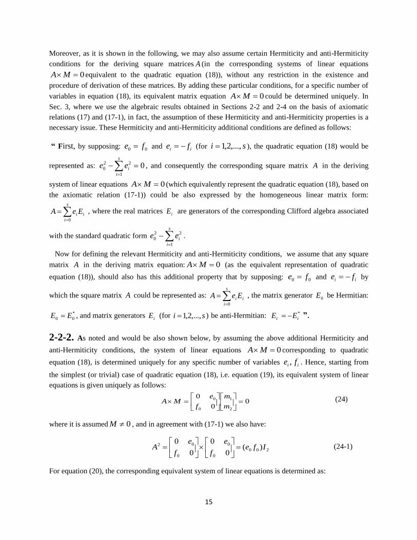
Moreover, as it is shown in the following, we may also assume certain Hermiticity and anti-Hermiticity

conditions for the deriving square matrices A (in the corresponding systems of linear equations

0MA equivalent to the quadratic equation (18)), without any restriction in the existence and

procedure of derivation of these matrices. By adding these particular conditions, for a specific number of

variables in equation (18), its equivalent matrix equation 0MA could be determined uniquely. In

Sec. 3, where we use the algebraic results obtained in Sections 2-2 and 2-4 on the basis of axiomatic

relations (17) and (17-1), in fact, the assumption of these Hermiticity and anti-Hermiticity properties is a

necessary issue. These Hermiticity and anti-Hermiticity additional conditions are defined as follows:

“ First, by supposing: 00 fe and ii fe (for si ,...,2,1 ), the quadratic equation (18) would be

represented as: 01

22

0

s

i

iee , and consequently the corresponding square matrix A in the deriving

system of linear equations 0MA (which equivalently represent the quadratic equation (18), based on

the axiomatic relation (17-1)) could be also expressed by the homogeneous linear matrix form:

s

i

ii EeA0

, where the real matrices iE are generators of the corresponding Clifford algebra associated

with the standard quadratic form

s

i

iee1

22

0 .

Now for defining the relevant Hermiticity and anti-Hermiticity conditions, we assume that any square

matrix A in the deriving matrix equation: 0MA (as the equivalent representation of quadratic

equation (18)), should also has this additional property that by supposing: 00 fe and ii fe by

which the square matrix A could be represented as:

s

i

ii EeA0

, the matrix generator 0E be Hermitian:

*

00 EE , and matrix generators iE (for si ,...,2,1 ) be anti-Hermitian: *

ii EE ”.

2-2-2. As noted and would be also shown below, by assuming the above additional Hermiticity and

anti-Hermiticity conditions, the system of linear equations 0MA corresponding to quadratic

equation (18), is determined uniquely for any specific number of variables ii fe , . Hence, starting from

the simplest (or trivial) case of quadratic equation (18), i.e. equation (19), its equivalent system of linear

equations is given uniquely as follows:

00

0

2

1

0

0

m

m

f

eMA (24)

where it is assumed 0M , and in agreement with (17-1) we also have:

200

0

0

0

02 )(0

0

0

0Ife

f

e

f

eA

(24-1)

For equation (20), the corresponding equivalent system of linear equations is determined as:

16

0

00

00

00

00

0

0

3

2

1

01

10

01

10

m

m

m

m

ee

ff

fe

fe

M

M

A

AMA

(25)

where we have:

41100

01

10

01

10

01

10

01

10

2 )(

00

00

00

00

00

00

00

00

,0 Ifefe

ee

ff

fe

fe

ee

ff

fe

fe

AM

MM

(25-1)

Notice that matrix equation (25) could be represented by two matrix equations, as follows:

,03

01

10

m

m

fe

feMA (25-2)

02

1

01

10

m

m

ee

ffMA (25-3)

The matrix equations (25-2) and (25-3) are equivalent (due to the assumption of arbitrariness of

parameters mmmm ,,, 321 ), so we may choose the matrix equation (25-2) as the system of linear

equations equivalent to the quadratic equation (20) – where for simplicity in the indices of parameters im ,

we may simply replace arbitrary parameter 3m with arbitrary parameter 1m , as follows (for 01

m

m ):

.01

01

10

m

m

fe

fe (26)

The system of linear equations corresponding to the quadratic equation (21) is obtained as:

,0

00000

00000

00000

00000

00000

00000

00000

00000

0

0

7

6

5

4

3

2

1

021

012

210

120

021

012

210

120

m

m

m

m

m

m

m

m

eee

eff

fef

fef

fee

fff

fee

fee

M

M

A

AMA

(27)

where in agreement with (17) we have:

8221100

021

012

210

120

021

012

210

120

021

012

210

120

021

012

210

120

2

)(

1)-(27

00000

00000

00000

00000

00000

00000

00000

00000

00000

00000

00000

00000

00000

00000

00000

00000

Ifefefe

eee

eff

fef

fef

fee

fff

fee

fee

eee

eff

fef

fef

fee

fff

fee

fee

A

17

In addition, similar to equation (25), the obtained matrix equation (27) is equivalent to a system of two

matrix equations, as follows:

,0

0

0

0

0

7

6

5

021

012

210

120

m

m

m

m

fee

fff

fee

fee

MA (27-2)

0

0

0

0

0

4

3

2

1

021

012

210

120

m

m

m

m

eee

eff

fef

fef

MA (27-3)

The matrix equations (27-2) and (27-3) are equivalent (due to the assumption of arbitrariness of

parameters mmmm ,,...,, 721 ), so we may choose the equation (27-2) as the system of linear equations

corresponding to the quadratic equation (21) – where for simplicity in the indices of parameters im , we

may simply replace the arbitrary parameters 5m , 6m , 7m with parameters 1m , 2m , 3m , as follows:

.0 ,0

0

0

0

0

3

2

1

3

2

1

021

012

210

120

m

m

m

m

m

m

m

m

fee

fff

fee

fee

(28)

Similarly, for the quadratic equations (22) the corresponding system of linear equations is obtained

uniquely as follows:

0

0000

0000

0000

0000

0000

0000

0000

0000

7

6

5

4

3

2

1

0321

0312

0213

0123

3210

3120

2130

1230

m

m

m

m

m

m

m

m

feee

feff

feff

feff

fffe

feee

feee

feee

(29)

where the column parametric matrix M in (29) is non-zero 0M .

In a similar manner, the uniquely obtained system of linear equations corresponding to the quadratic

equation (23), is given by:

18

0

00000000000

00000000000

00000000000

00000000000

00000000000

00000000000

00000000000

00000000000

00000000000

00000000000

00000000000

00000000000

00000000000

00000000000

00000000000

00000000000

15

14

13

12

11

10

9

8

7

6

5

4

3

2

1

04321

04312

04213

04123

03214

03124

02134

01234

43210

43120

42130

41230

32140

31240

21340

12340

m

m

m

m

m

m

m

m

m

m

m

m

m

m

m

m

feeee

feeff

feeff

feeff

feeff

feeff

feeff

fffff

fffee

fffee

fffee

feeee

fffee

feeee

feeee

feeee

(30)

where we‘ve assumed the parametric column matrix M in (30) is non-zero, 0M .

In a similar manner, the systems of linear equations (written in matrix forms similar to the matrix

equations (24), (26), (28), (29) and (30)) with larger sizes are obtained for the quadratic equation (18) in

more variables (i.e. for ,...8,7,6s ), where the size of the square matrices of the corresponding matrix

equations is ss 22 (which could be reduced to

11 22 ss for 2s ). In general (as it has been also

mentioned in Sec. 2-1), the size of the nn square matrices A (with the minimum value for n ) in the

matrix equations 0MA corresponding to the homogeneous polynomials ),...,,,( 321 sbbbbF of

degree r defined in axiom (17) is ss rr (which for 2r this size, in particular, could be reduced to

11 22 ss). Moreover, based on the axiom (17), in fact, by solving the obtained system of linear

equations corresponding to a homogeneous equation of degree r , we may systematically show (and

decide) whether this equation has the integral solution.

2-3. Similar to the uniquely obtained systems of linear equations corresponding to the homogeneous

quadratic equations (in Sec. 2-2), in this section in agreement with the axiom (17), we present the

obtained systems of linear equations, i.e. 0MA (by assuming the minimum value for n , i.e. the

size of square matrix nnA ), corresponding to some homogeneous equations of degrees 3, 4 and 5,

respectively. For the homogeneous equation of degree three of the type:

,0),,,,,( 111

2

222

2

2

2

000

2

0221100 gfefefefefefefefeF (31)

the corresponding system of linear equations is given as follows:

19

,0

:::00

00

00

27

2

1

3

2

1

m

m

m

A

A

A

MA (32)

where A is a 27×27 square matrix written in terms of the square 9×9 matrices 21, AA and 3A , given by:

,

000000

000000

000000

000000

000000

000000

000000

000000

000000

2001

210

210

201

2100

210

0122

1022

10022

1

ffef

fgf

fee

eef

egfe

eef

fffe

gefe

efefe

A

,

000000

000000

000000

000000

000000

000000

000000

000000

000000

2001

210

210

2201

22100

2210

012

102

1002

2

efef

egf

eee

feef

fegfe

feef

fff

gef

efef

A

22001

2210

2210

201

2100

210

012

102

1002

3

000000

000000

000000

000000

000000

000000

000000

000000

000000

fefef

fegf

feee

fef

fgfe

fef

ffe

gee

efee

A . (33)

The uniquely obtained system of linear equations (i.e. 0MA , by assuming the minimum size for the

square matrix nnA ) corresponding to the well-known homogeneous equation of degree three:

0)(2),,( 333 BbcacbaF (34)

20

has the following form (in compatible with the new axiom (17)):

,0

:::00

00

00

27

2

1

3

2

1

m

m

m

A

A

A

MA (35)

where A is a 27×27 square matrix written in terms of the 9×9 matrices 1A , 2A and 3A given by:

(36)

For the 4th degree homogeneous equation of the type:

0),,,,,( 43212

3

1

3

21432121 ffffeeeeffffeeF (37)

the corresponding system of linear equations is given as,

,0

:::

000

000

000

000

16

2

1

4

3

2

1

m

m

m

A

A

A

A

MA (38)

where A is a 16×16 square matrix represented in terms of the 4×4 matrices 4321 ,,, AAAA :

21

(39)

In addition, the system of linear equations corresponding to 5th degree homogeneous equation of the type,

0),,,,,,( 54321

4

21

3

2

2

1

2

2

3

12

4

15432121 fffffeeeeeeeefffffeeF (40)

is determined as:

,0

:::

0000

0000

0000

0000

0000

25

3

2

1

5

4

3

2

1

m

m

m

m

A

A

A

A

A

MA (41)

where A is a 25×25 square matrix expressed in terms of the following 5×5 matrices 54321 ,,,, AAAAA :

(42)

2-4. In this Section by solving the derived systems of linear equations (26), (28), (29) and (30)

corresponding to the quadratic homogeneous equations (20) – (23) in Sec. 2-2, the general parametric

solutions of these equations are obtained for unknowns ie and if . There are the standard methods for

22

obtaining the general solutions of the systems of homogeneous linear equations in integers [7, 8]. Using

these methods, for the system of linear equations (26) (and consequently, its corresponding quadratic

equation (20)) we get directly the following general parametric solutions for unknowns 10 ,ee and 10 , ff :

1011111000 ,,, mlkfmlkemlkfmlke (43)

where 10 ,kk , lmm ,,1 are arbitrary parameters. In the matrix representation the general parametric

solution (43) has the following form:

1

0

1

1

1

0

1

0

1

0

0

0,

10

01

k

k

m

mlKlM

f

f

k

klmKlM

e

efe

(43-1)

where 2mIM e , K is a column parametric matrix and fM is also a parametric anti-symmetric matrix.

For the system of linear equations (28) (and, consequently, for its corresponding quadratic homogeneous

equation (21)), the following general parametric solution is obtained directly:

)(,),(,),(, 312022210321112211000 mkmklfmlkemkmklfmlkemkmklfmlke (44)

where lmmmmkkk ,,,,,,, 321210 are arbitrary parameters. In matrix representation the general parametric

solution (44) could be also written as follows:

2

1

0

32

31

21

2

1

0

2

1

0

2

1

0

0

0

0

,

100

010

001

k

k

k

mm

mm

mm

lKlM

f

f

f

k

k

k

lmKlM

e

e

e

fe (44-1)

where 3mIM e , K is a column parametric matrix and fM is also a parametric anti-symmetric matrix.

In addition, it could be simply shown that by adding two particular solutions of the types },{ ii fe and

},{ ii fe of homogeneous quadratic equation (18), the new solution },{ iii fee is also obtained, as

follows:

0)(0)()0,0(0000

s

i

iii

s

i

iiii

s

i

ii

s

i

ii feefefefefe (44-2)

Using the general basic property (44-2) in addition to the general parametric solution (44) of quadratic

equation (21) (which has been obtained directly from the system of linear equations (28) corresponding to

quadratic equation (21)), exceptionally, the following equivalent general parametric solution is also

obtained for quadratic equation (21):

)(),(),(

),(),(),(

3120212210321

21122110300

mkmklfkmmklemkmklf

kmmklemkmklfkmmkle

(45)

where kkkk ,,, 210 , lmmmm ,,,, 321 are arbitrary parameters.

Moreover, the parametric solution (45) by the direct bijective replacements of six unknown variables

),( ii fe (where i = 0,1,2) with the six new variables of the type h , given by:

23

,,,, 100212201230 hfhehehe 032311 , hfhf , in addition to the replacements of nine

arbitrary parameters 3210 ,,, uuuu , wvvvv ,,,, 3210 , with new nine parameters of the types 3210 ,,, uuuu ,

wvvvv ,,,, 3210 , given as: ,,,, 2120130 ukukukuk ,2uk ,11 vm ,02 vm ,33 vm

,2vm wl , exceptionally, could be also represented as follows:

);(),(),(

),(),(),(

300303122121133131

022020011010322323

vuvuwhvuvuwhvuvuwh

vuvuwhvuvuwhvuvuwh

(45-1)

where it could be expressed by a single uniform formula as well (for μ, ν = 0,1,2,3):

)( vuvuwh (45-2)

A crucial and important issue concerning the algebraic representation (45-2) (as the differences of

products of two parametric variables u and v ) for the general parametric solution (45), is that it

generates a symmetric algebra Sym(V) on the vector space ,V where Vvu ),( [11]. This essential

property of the form (45-2) would be used for various purposes in the following and also in Sec. 3 (where

we show the applications of this axiomatic linearization-parameterization approach and the results

obtained in this Section and Sec. 2-4, in foundations of physics).

In addition, as it is also shown in the following, it should be mentioned again that the algebraic form

(45-2) (representing the symmetric algebra Sym(V)), exceptionally, is determined solely from the

parametric solution (44-1) (obtained from the system of equations (28)) by using the identity (44-2). In

fact, from the parametric solutions obtained directly from the subsequent systems of linear equations. i.e.

equations (29), (30) and so on (corresponding to the quadratic equations (22), (23),…, and subsequent

equations, i.e. 00

s

i

ii fe for 3s ), the expanded parametric solutions of the type (45) (equivalent to

the algebraic form (45-2)) are not derived.

In the following (also see Ref. [76]), we present the parametric solutions that are obtained directly from

the systems of linear equations (29), (30) and so on, which also would be the parametric solutions of their

corresponding quadratic equations (18) in various number of unknowns (on the basis of axiom (17)).

Meanwhile, the following obtained parametric solutions for the systems of linear equations (29), (30) and

so on, similar to the parametric solutions (43) and (44), include one parametric term for each of

unknowns ie , and sum of s parametric terms for each of unknowns if (where si ,...,3,2,1,0 ).

Hence, the following parametric solution is derived directly from the system of linear equations (29) (that

would be also the solution of its corresponding quadratic equation (22)):

).(,),(,

),(,),(,

615230333715320222

726310111332211000

mkmkmklfmlkemkmkmklfmlke

mkmkmklfmlkemkmkmklfmlke

(46)

where lkkkk ,,,, 3210 are arbitrary parameters. In the matrix representation, the parametric solution (46)

is represented as follows:

24

3

2

1

0

563

572

671

321

3

2

1

0

3

2

1

0

3

2

1

0

0

0

0,

1000

0100

0010

0001

k

k

k

k

mmm

mmm

mmm

mmmo

lKlM

f

f

f

f

k

k

k

k

lmKlM

e

e

e

e

fe (46-1)

where 4mIM e , K is a column parametric matrix and fM is also a parametric anti-symmetric matrix.

However, in solutions (46) or (46-1) the parameters mmmmmmmm ,,,,,,, 7654321 are not arbitrary, and in

fact, in the course of obtaining the solution (46) from the system of linear equations (29), a condition

appears for these parameters as follows:

07362514 mmmmmmmm (47)

The condition (47) is also a homogeneous quadratic equation that should be solved first, in order to obtain

a general parametric solution for the system of linear equations (29). Since the parameter 4m has not

appeared in the solution (46), it could be assumed that 04 m , and the condition (47) is reduced to the

following homogeneous quadratic equation, which is equivalent to the quadratic equation (20)

(corresponding to the system of linear equations (28)):

,04 m 0736251 mmmmmm , (47-1)

where the parameter m would be arbitrary. The condition (47-1) is equivalent to the quadratic equation

(21). Hence by using the general parametric solution (45-1) (as the most symmetric solution obtained for

quadratic equation (21) by solving its corresponding system of linear equations (28)), the following

general parametric solution for the condition (47-1) is obtained:

)(),(),(

),(),(),(

211271331632235

033030220201101

vuvuwmvuvuwmvuvuwm

vuvuwmvuvuwmvuvuwm

(48)

where 3210 ,,, uuuu , wvvvv ,,,, 3210 , m are arbitrary parameters. Now by replacing the solutions (48)

(obtained for 765321 ,,,,, mmmmmm in terms of the new parameters 3210 ,,, uuuu , wvvvv ,,,, 3210 ) in the

relations (46), the general parametric solution of the system of linear equations (29) (and its

corresponding quadratic equation (22)) is obtained in terms of the arbitrary parameters 3210 ,,, kkkk ,

3210 ,,, uuuu , ,,,,, 3210 wvvvv lm, .

For the system of linear equations (30) (and its corresponding quadratic equation (23)), the following parametric solution is obtained:

)(,

),(,),(,

),(,),(,

12111210350444

1411321043033315113311420222

1521431241011154332211000

mkmkmkmklfmlke

mkmkmkmklfmlkemkmkmkmklfmlke

mkmkmkmklfmlkemkmkmkmklfmlke

(49)

where lkkkkk ,,,,, 43210 are arbitrary parameters. In the matrix representation the solution (49) could be

also written as follows:

25

4

3

2

1

0

1011125

1013143

1113152

1214151

5321

4

3

2

1

0

4

3

2

1

0

4

3

2

1

0

0

0

0

0

0

,

10000

01000

00100

00010

00001

k

k

k

k

k

mmmm

mmmm

mmmm

mmmm

mmmm

lKlM

f

f

f

f

f

k

k

k

k

k

lmKlM

e

e

e

e

e

fe (49-1)

where 5mIM e , K is a column parametric matrix and fM is also a parametric anti-symmetric matrix.

However, similar to the system of equations (29), in the course of obtaining the solutions (49) or (49-1)

from the system of linear equations (30), the following conditions appear for parameters

1514131211105321 ,,,,,,,,, mmmmmmmmmm :

.

,

,

,

,

1312141115109

1351131028

1451231017

1551221116

1531421314

mmmmmmmm

mmmmmmmm

mmmmmmmm

mmmmmmmm

mmmmmmmm

(50)

that is similar to the condition (47). Here also by the same approach, since the parameters

98764 ,,,, mmmmm

have not appeared in the solution (49), it could be assumed that

098764 mmmmm , and the set of conditions (50) are reduced to the following system of

homogeneous quadratic equations which are similar to the quadratic equation (20) (corresponding to the

system of linear equations (28)):

;0

,0

,0

,0

,0

,0

141113121510

113135102

153142131

155122111

145123101

98764

mmmmmm

mmmmmm

mmmmmm

mmmmmm

mmmmmm

mmmmm

(50-1)

The conditions (50-1) are also similar to the quadratic equation (21). Hence using again the general

parametric solution (45-1), the following general parametric solutions for the system of homogeneous

quadratic equations (50-1) are obtained directly:

).(),(

),(),(

),(),(

,0,0,0

,0),(

,0),(

),(),(

122115133114

233213144112

244211344310

987

640045

403303

2002201101

vuvuwmvuvuwm

vuvuwmvuvuwm

vuvuwmvuvuwm

mmm

mvuvuwm

mvuvuwm

vuvuwmvuvuwm

(51)

26

where 4321043210 ,,,,,,,,, vvvvvuuuuu and w are arbitrary parameters. Now by replacing the solution

(51) (that have been obtained for 321 ,, mmm 1514131211105 ,,,,,,, mmmmmmm in terms of the new

parameters wvvvvvuuuuu ,,,,,,,,,, 4321043210 ) in the relations (49), the general parametric solution of

the system of linear equations (30) (and its corresponding quadratic equation (23)) is obtained in terms of

the arbitrary parameters ,,,,,,,,,,,,,,,, 432104321043210 wvvvvvuuuuukkkkk lm, .

Meanwhile, similar to the relations (48) and (51), it should be noted that arbitrary parameter 1m in the

general parametric solution (43) and arbitrary parameters 321 ,, mmm in the general parametric solution

(44) (which have been obtained as the solutions of quadratic equations (20) and (21), respectively, by

solving their equivalent systems of linear equations (26) and (28)), by keeping their arbitrariness property,

could particularly be expressed in terms of new arbitrary parameters 1010 ,,, vvuu and 210210 ,,,,, vvvuuu ,

as follows, respectively:

);( 01101 vuvuwm (43-2)

).(),(),( 033030220201101 vuvuwmvuvuwmvuvuwm (44-3)

In fact, as a particular common algebraic property of both parametric relations (43-2) and (44-2), it could

be shown directly that by choosing appropriate integer values for parameters wvvuu ,,,, 1010 in the

relation (43-2), the parameter 1m (defined in terms of arbitrary parameters ),,,, 1010 wvvuu could take any

given integer value, and similarly, by choosing appropriate integer values for parameters

wvvvuuu ,,,,,, 210210 in the relation (43-2), the parameters 321 ,, mmm (defined in terms of arbitrary

parameters ),,,,,, 210210 wvvvuuu could also take any given integer values. Therefore, using this common

algebraic property of the parametric relations (43-2) and (44-2), the arbitrary parameter 1m in general

parametric solutions (43), and arbitrary parameters 321 ,, mmm in general parametric solutions (44), could

be equivalently replaced by new arbitrary parameters wvvuu ,,,, 1010 and wvvvuuu ,,,,,, 210210 ,

respectively. In addition, for the general quadratic homogeneous equation (18) with more number of

unknowns, the general parametric solutions could be obtained by the same approaches used above for

quadratic equations (20) – (23), i.e. by solving their corresponding systems of linear equations (defined on

the basis of axiom (17)). Moreover, using the isomorphic transformations (18-3) and the above general

parametric solutions obtained for quadratic equations (20) – (23),… (via solving their corresponding

systems of linear equations (26), (28), (29), (30),…), the general parametric solutions of quadratic

equations of the regular type (18-2) (in various number of unknown) are also obtained straightforwardly.

All the parametric solutions that are obtained by this new systematic matrix approach for the

homogeneous quadratic equations and also higher degree homogeneous equations of the type

0),...,,,( 321 sxxxxF (defined in the axiom (17)), are fully compatible with the solutions and

conclusions that have been obtained previously for various homogeneous equations by different and

miscellaneous methods and approaches [6, 7, 8]. In Sec. 3, we‘ve used the uniquely specified systems of

homogeneous linear equations (and also their general parametric solutions) corresponding to the

homogeneous quadratic equations – where, in particular, it has been assumed basically that the

components of the relativistic energy-momentum vector (as one of the most basic physical quantities) in

the Lorentz invariant energy-momentum (homogeneous) quadratic relation, can only take the rational

values.

27

3. A Unique Mathematical Derivation of the Laws Governing the Fundamental

Forces of Nature: Based on a New Algebraic-Axiomatic (Matrix) Approach

In this Section, , as a new mathematical approach to origin of the laws of nature, using the new basic

algebraic axiomatic (matrix) formalism (presented in Sec.2), “it is shown that certain mathematical

forms of fundamental laws of nature, including laws governing the fundamental forces of nature

(represented by a set of two definite classes of general covariant massive field equations, with new

matrix formalisms), are derived uniquely from only a very few axioms”; where in agreement with the

rational Lorentz group, it is also basically assumed that the components of relativistic energy-

momentum can only take rational values. Concerning the basic assumption of rationality of

relativistic energy-momentum, it is necessary to note that the rational Lorentz symmetry group is not

only dense in the general form of Lorentz group, but also is compatible with the necessary conditions

required basically for the formalism of a consistent relativistic quantum theory [77]. In essence, the

main scheme of this new mathematical axiomatic approach to fundamental laws of nature is as

follows. First in Sec. 3-1-1, based on the assumption of rationality of D-momentum, by linearization

(along with a parameterization procedure) of the Lorentz invariant energy-momentum quadratic

relation, a unique set of Lorentz invariant systems of homogeneous linear equations (with matrix

formalisms compatible with certain Clifford, and symmetric algebras) is derived. Then in Sec. 3-4,

by first quantization (followed by a basic procedure of minimal coupling to space-time geometry) of

these determined systems of linear equations, a set of two classes of general covariant massive

(tensor) field equations (with matrix formalisms compatible with certain Clifford, and Weyl algebras)

is derived uniquely as well. Each class of the derived general covariant field equations also includes a

definite form of torsion field appeared as generator of the corresponding field‘ invariant mass. In

addition, in Sections 3-4 – 3-5, it is shown that the (1+3)-dimensional cases of two classes of derived

field equations represent a new general covariant massive formalism of bispinor fields of spin-2, and

spin-1 particles, respectively. In fact, these uniquely determined bispinor fields represent a unique set

of new generalized massive forms of the laws governing the fundamental forces of nature, including

the Einstein (gravitational), Maxwell (electromagnetic) and Yang-Mills (nuclear) field equations.

Moreover, it is also shown that the (1+2)-dimensional cases of two classes of these field equations

represent (asymptotically) a new general covariant massive formalism of bispinor fields of spin-3/2

and spin-1/2 particles, respectively, corresponding to the Dirac and Rarita–Schwinger equations. As a particular consequence, in Sec. 3-4-2, it is shown that a certain massive formalism of general

relativity – with a definite form of torsion field appeared originally as the generator of gravitational

field‘s invariant mass – is obtained only by first quantization (followed by a basic procedure of

minimal coupling to space-time geometry) of a certain set of special relativistic algebraic matrix

equations. In Sec. 3-4-4, it has been also proved that Lagrangian densities specified for the originally

derived new massive forms of the Maxwell, Yang-Mills and Dirac field equations, are also gauge

invariant, where the invariant mass of each field is generated solely by the corresponding torsion

field. In addition, in Sec. 3-4-5, in agreement with recent astronomical data, a particular new form of

massive boson is identified (corresponding to U(1) gauge group) with invariant mass:

mγ ≈ 4.90571×10-50kg, generated by a coupled torsion field of the background space-time geometry.

Moreover, in Sec. 3-5-2, based on the definite mathematical formalism of this axiomatic approach,

along with the C, P and T symmetries (represented basically by the corresponding quantum

28

operators) of the fundamentally derived field equations, it has been concluded that the universe could

be realized solely with the (1+2) and (1+3)-dimensional space-times (where this conclusion, in

particular, is based on the time-reversal symmetry). In Sections 3-5-3 and 3-5-4, it is proved that

'CPT' is the only (unique) combination of C, P, and T symmetries that could be defined as a

symmetry for interacting fields. In addition, in Sec. 3-5-4, on the basis of these discrete symmetries

of derived field equations, it has been also shown that only left-handed particle fields (along with

their complementary right-handed fields) could be coupled to the corresponding (any) source

currents. Furthermore, in Sec. 3-6, it has been shown that metric of the background space-time is

diagonalized for the uniquely derived fermion field equations (defined and expressed solely in (1+2)-

dimensional space-time), where this property generates a certain set of additional symmetries

corresponding uniquely to the SU(2)LU(2)R symmetry group for spin-1/2 fermion fields

(representing ―1+3‖ generations of four fermions, including a group of eight leptons and a group of

eight quarks), and also the SU(2)LU(2)R and SU(3) gauge symmetry groups for spin-1 boson fields

coupled to the spin-1/2 fermionic source currents. Hence, along with the known elementary particles,

eight new elementary particles, including: four new charge-less right-handed spin-1/2 fermions (two

leptons and two quarks, represented by ―ze , zn and zu , zd‖), a spin-3/2 fermion, and also three new

spin-1 massive bosons (represented by ",~

,~

" ZWW

, where in particular, the new boson Z

is

complementary right-handed particle of ordinary Z boson), are predicted uniquely by this new

mathematical axiomatic approach.

Furthermore, as a particular result, in Sec. 3-4-2, based on the definite and unique formulation of the

derived Maxwell‘s equations (and also determined Yang-Mills equations, represented uniquely with

two specific forms of gauge symmetries, in 3-6-3-2), it is also concluded generally that magnetic

monopoles could not exist in nature.

3-1. As noted in Sec. 1-1, the main results obtained in this article are based on the following three

basic assumptions (as postulates):

(1)- “A new definite axiomatic generalization of the axiom of ―no zero divisors‖ of integral

domains (including the integr ring ℤ) is assumed (represented by formula (17), in Sec. 2-1);”

This basic assumption (as a postulate) is a new mathematical concept. In Sec. 2-1, based on this

new axiom, a general algebraic axiomatic (matrix) approach (in the form of a basic linearization-

parameterization theory) to homogeneous equations of degree r ≥ 2 (over the integer domain,

extendable to field of rational numbers), has been formulated. A summary of the main results

obtained from this axiomatic approach have been presented in Sec. 1-1. As particular outcome of this

new mathematical axiomatic formalism (based on the axiomatic relations (17) and (17-1), including

their basic algebraic properties presented in detail, in Sections 2-1 – 2-4), in Sec. 3-4, it is shown that

using, a unique set of general covariant massive (tensor) field equations (with new matrix formalism

compatible with Clifford, and Weyl algebras), corresponding to the fundamental field equations of

physics, are derived – where, in agreement with the rational Lorentz symmetry group, it has been

basically assumed that the components of relativistic energy-momentum can only take the rational

values. In Sections 3-2 – 3-6, we present in detail the main applications of this basic algebraic

assumption (along with the following basic assumptions (2) and (3)) in fundamental physics.

29

(2)- “In agreement with the rational Lorentz symmetry group, we assume basically that the

components of relativistic energy-momentum (D-momentum) can only take the rational values;”

Concerning this assumption, it is necessary to note that the rational Lorentz symmetry group is

not only dense in the general form of Lorentz group, but also is compatible with the necessary

conditions required basically for the formalism of a consistent relativistic quantum theory [77].

Moreover, this assumption is clearly also compatible with any quantum circumstance in which the

energy-momentum of a relativistic particle is transferred as integer multiples of the quantum of

action ―h‖ (Planck constant).

Before defining the next basic assumption, it should be noted that from the basic assumptions (1) and

(2), it follows directly that the Lorentz invariant energy-momentum quadratic relation (represented by

formula (52), in Sec. 3-1-1) is a particular form of homogeneous quadratic equation (18-2). Hence, using

the set of systems of linear equations that have been determined uniquely as equivalent algebraic

representations of the corresponding set of quadratic homogeneous equations (given by equation (18-2) in

various number of unknown variables, respectively), a unique set of the Lorentz invariant systems of

homogeneous linear equations (with matrix formalisms compatible with certain Clifford, and

symmetric algebras) are also determined, representing equivalent algebraic forms of the energy-

momentum quadratic relation in various space-time dimensions, respectively. Subsequently, we‘ve shown

that by first quantization (followed by a basic procedure of minimal coupling to space-time

geometry) of these determined systems of linear equations, a unique set of two definite classes of

general covariant massive (tensor) field equations (with matrix formalisms compatible with certain

Clifford, and Weyl algebras) is also derived, corresponding to various space-time dimensions,

respectively. In addition, it is also shown that this derived set of two classes of general covariant field

equations represent new tensor massive (matrix) formalism of the fundamental field equations of physics,

corresponding to fundamental laws of nature (including the laws governing the fundamental forces of

nature). Following these essential results, in addition to the basic assumptions (1) and (2), it would be

also basically assumed that:

(3)- “We assume that the mathematical formalism of the fundamental laws of nature, are

defined solely by the axiomatic matrix constitution formulated uniquely on the basis of

postulates (1) and (2)”.

In addition to this basic assumption, in Sec. 3-5, the C, P and T symmetries of uniquely derived

general covariant field equations (that are equations (71) and (72), in Sec. 3-4), are also represented

basically by their corresponding quantum matrix operators.

3-1-1. Based on the basic assumption (2), i.e., the assumption of rationality of the relativistic energy-

momentum, the following Lorentz invariant quadratic relations (expressed in terms of the components of

D-momentums p ,

p of a relativistic massive particle (given in two reference frames), and also

components of quantity kmp 0

st , where m0 is the invariant mass of particle and k is its covariant

velocity in the stationary reference frame):

,ppgppg

(51)

30

stst

νμμν

νμμν ppgppg (52)

.)()())(( 2

0

2

00

00

00 cmkmgkmkmg νμμν

would be particular cases of homogeneous quadratic equation (18-2) in Sec. 2-2, and hence, they would

be necessarily subject to the process of linearization (along with a parameterization procedure), using the

systematic axiomatic approach presented Sections 2, 2-2 and 2-4 (formulated based on the basic

assumption (1)).

The Lorentz invariant relations (51) and (52) (as the norm of the relativistic energy-momentum) have

been defined in the D-dimensional space-time, where m0 is the invariant mass of the particle, p and p

are its relativistic energy-momentums (i.e. D-momentums) given respectively in two reference frames, k

is a time-like covariant vector given by: )0,...,0,()0,...,0,( 00

0 gckk , ―c‖ is the speed of light, and

the components of metric have the constant values. As noted in Sec. 1-2, in this article, the sign

conventions (2) (including the metric signature (+ – – …– )) and geometric units would be used (where in

particular ―c = 1‖). However, for the clarity, in some of relativistic formulas (such as the relativistic

matrix relations), the speed of light ―c‖ is indicated formally. As a crucial issue here, it should be noted that in the invariant quadratic relations (51) and (52), the

components of metric which have the constant values (as assumed), necessarily, have been written by

their general representations g (and not by the Minkowski metric

, and so on). This follows from

the fact that by axiomatic approach of linearization-parameterization (presented in Sections 2-1 – 2-4) of

quadratic relations (51) and (52) (as particular forms of homogeneous quadratic equation (18-2) which

could be expressed equivalently by quadratic equations of the types (18) via the linear transformations

(18-3)), their corresponding algebraic equivalent systems of linear equations could be determined

uniquely. In fact, based on the formulations of systems of linear equations obtained uniquely for the

quadratic equations (18) in Sections 2-2 – 2-4, it is concluded directly that the algebraic equivalent

systems of linear equations corresponding to the relations (51) and (52), are determined uniquely if and

only if these quadratic relations be expressed in terms of the components g represented by their general

forms (and not in terms of any special presentation of the metric‘s components, such as the Minkowski

metric, and so on). However, after the derivation of corresponding systems of linear equations

(representing uniquely the equivalent algebraic matrix forms of the quadratic relations (51) and (52) in

various space-time dimensions), the Minkowski metric could be used in these equations (and the

subsequent relativistic equations and relations as well). Hence, using the systems of linear equations (24), (26), (28), (29), (30),…, obtained uniquely on the basis

of the axiom (17) by linearization (along with a parameterization procedure) of the homogeneous

quadratic equations (19) – (23),… (which could be transformed directly to the general quadratic equation

(18-2), by the isomorphic linear transformations (18-3)), and also using the parametric relations (43-2),

(44-3), (48) and (52) (expressed in terms of the arbitrary parameters u and v ), as the result of

linearization (along with a parameterization procedure) of the invariant quadratic relations (51) and (52),

the following systems of linear equations are also derived uniquely corresponding to various space-time

dimensions, respectively:

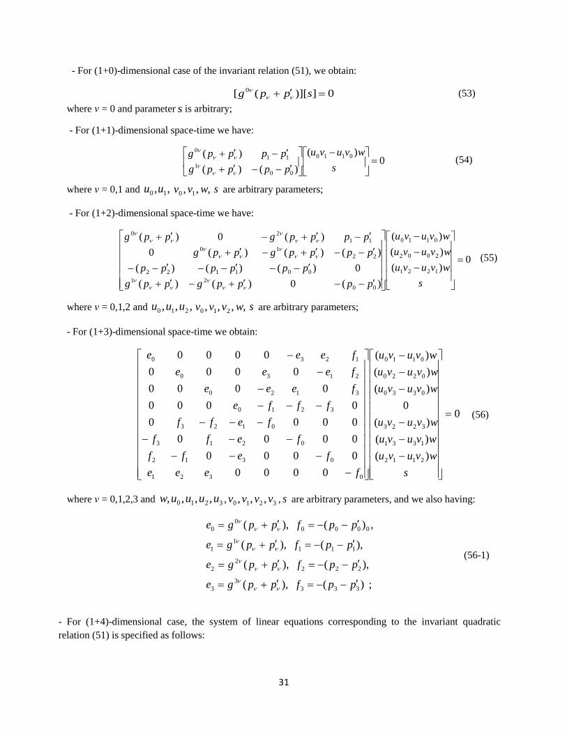
31

- For (1+0)-dimensional case of the invariant relation (51), we obtain:

0])][([ 0 sppg

(53)

where ν = 0 and parameter s is arbitrary; - For (1+1)-dimensional space-time we have:

0)(

)()(

)( 0110

00

1

11

0

s

wvuvu

ppppg

ppppg

(54)

where ν = 0,1 and ,, 10 uu ,,, 10 wvv s are arbitrary parameters; - For (1+2)-dimensional space-time we have:

0)(

)(

)(

)(0)()(

0)()()(

)()()(0

)(0)(

1221

2002

0110

00

21

001122

22

10

11

20

s

wvuvu

wvuvu

wvuvu

ppppgppg

pppppp

ppppgppg

ppppgppg

(55)

where ν = 0,1,2 and ,,, 210 uuu ,,,, 210 wvvv s are arbitrary parameters;

- For (1+3)-dimensional space-time we obtain:

0

)(

)(

)(

0

)(

)(

)(

0000

0000

0000

0000

0000

0000

0000

0000

2112

1331

3223

0330

0220

0110

0321

0312

0213

0123

3210

3120

2130

1230

s

wvuvu

wvuvu

wvuvu

wvuvu

wvuvu

wvuvu

feee

feff

feff

feff

fffe

feee

feee

feee

(56)

where ν = 0,1,2,3 and 3210 ,,,, uuuuw , 3210 ,,, vvvv , s are arbitrary parameters, and we also having:

;)(),(

),(),(

),(),(

,)(),(

333

3

3

222

2

2

111

1

1

0000

0

0

ppfppge

ppfppge

ppfppge

ppfppge

(56-1)

- For (1+4)-dimensional case, the system of linear equations corresponding to the invariant quadratic

relation (51) is specified as follows:

32

0

)(

)(

)(

)(

)(

)(

0

0

0

0

)(

0

)(

)(

)(

00000000000

00000000000

00000000000

00000000000

00000000000

00000000000

00000000000

00000000000

00000000000

00000000000

00000000000

00000000000

00000000000

00000000000

00000000000

00000000000

1221

1331

2332

1441

2442

3443

4004

0330

2002

0110

04321

04312

04213

04123

03214

03124

02134

01234

43210

43120

42130

41230

32140

31240

21340

12340

s

wvuvu

wvuvu

wvuvu

wvuvu

wvuvu

wvuvu

wvuvu

wvuvu

wvuvu

wvuvu

feeee

feeff

feeff

feeff

feeff

feeff

feeff

fffff

fffee

fffee

fffee

feeee

fffee

feeee

feeee

feeee

(57)

where ν = 0,1,2,3,4 , 43210 ,,,, uuuuu , wvvvvv ,,,,, 43210 , s are arbitrary parameters, and we have:

;),(

,),(

,),(

,),(

,),(

444

4

4

333

3

3

222

2

2

111

1

1

000

0

0

ppfppge

ppfppge

ppfppge

ppfppge

ppfppge

(57-1)

The systems of linear equations that are obtained for (1+5) and higher dimensional cases of the invariant

quadratic relation (51), have also the formulations similar to the obtained systems of linear equations

(53) – (57), and would be expressed by the matrix product of a NN 22 square matrix and a 12 N

column

matrix in (1+ N)-dimensional space-time. For (1+5)-dimensional case of the invariant relation (51), the

column matrix of the corresponding system of linear equations (expressed by the matrix product of a

3232 square matrix and a 132 column matrix) is given by (where 543210 ,,,,, uuuuuu ,

swvvvvvv ,,,,,,, 543210 are arbitrary parameters):

33

.

)(

)(

)(

)(

)(

)(

0

)(

)(

)(

0

)(

0

0

0

,

0

0

0

0

0

0

0

)(

0

0

0

)(

0

)(

)(

)(

,

1221

3113

2332

4114

2442

4334

1551

5225

3553

5445

0550

0440

0330

0220

0110

s

wvuvu

wvuvu

wvuvu

wvuvu

wvuvu

wvuvu

wvuvu

wvuvu

wvuvu

wvuvu

Swvuvu

wvuvu

wvuvu

wvuvu

wvuvu

SS

SS

(57-2)

In a similar manner, using the axiomatic approach presented in Sec. 2, the systems of linear equations

corresponding to the energy-momentum invariant relation (52) in various space-time dimensions are

obtained uniquely as follows, respectively (note that by using the geometric units, we would take 1c ):

- For (1+0)-dimensional space-time we obtain:

000

0000

s

g

cmgpg

(58)

where ν = 0 and parameter s is arbitrary;

- For (1+1)-dimensional space-time we have:

0)(

))(()(

)(0110

00

00

00

0101

100

0000

s

wvuvu

g

cmp

g

cmgpg

pg

cmgpg

(59)

where ν = 0,1 and ,, 10 uu ,,, 10 wvv s are arbitrary parameters;

- For (1+2) dimensions we have (where ν = 0,1,2 and ,,, 210 uuu ,,,, 210 wvvv s are arbitrary parameters):

0)(

)(

)(

))((0)()(

0))((

)()(0

)(0)(

1221

2002

0110

00

00

00

0202

00

0101

00

0012

200

0101

00

0000

100

0202

00

0000

s

wvuvu

wvuvu

wvuvu

g

cmp

g

cmgpg

g

cmgpg

g

cmppp

pg

cmgpg

g

cmgpg

pg

cmgpg

g

cmgpg

(60)

34

- For (1+3)-dimensional space-time we obtain:

0

)(

)(

)(

0

)(

)(

)(

0000

0000

0000

0000

0000

0000

0000

0000

2112

1331

3223

0330

0220

0110

0321

0312

0213

0123

3210

3120

2130

1230

s

wvuvu

wvuvu

wvuvu

wvuvu

wvuvu

wvuvu

feee

feff

feff

feff

fffe

feee

feee

feee

(61)

where ν = 0,1,2,3 and 3210 ,,, uuuu , wvvvv ,,,, 3210 , s are arbitrary parameters, and we also having:

;),(

,),(

,),(

),(),(

33

00

0

303

3

22

00

0

202

2

11

00

0

101

1

00

000

00

0

000

0

pfgcmgpge

pfgcmgpge

pfgcmgpge

gcmpfgcmgpge

(61-1)

- For (1+4)-dimensional space-time, the system of linear equations corresponding to the invariant

quadratic relation (52) is derived as follows:

0

)(

)(

)(

)(

)(

)(

0

0

0

0

)(

0

)(

)(

)(

00000000000

00000000000

00000000000

00000000000

00000000000

00000000000

00000000000

00000000000

00000000000

00000000000

00000000000

00000000000

00000000000

00000000000

00000000000

00000000000

1221

1331

2332

1441

2442

3443

4004

0330

2002

0110

04321

04312

04213

04123

03214

03124

02134

01234

43210

43120

42130

41230

32140

31240

21340

12340

s

wvuvu

wvuvu

wvuvu

wvuvu

wvuvu

wvuvu

wvuvu

wvuvu

wvuvu

wvuvu

feeee

feeff

feeff

feeff

feeff

feeff

feeff

fffff

fffee

fffee

fffee

feeee

fffee

feeee

feeee

feeee

(62)

35

where ν = 0,1,2,3,4 and 43210 ,,,, uuuuu , wvvvvv ,,,,, 43210 , s are arbitrary parameters, and we have:

.),(

,),(

,),(

,),(

),(),(

44

00

0

404

4

33

00

0

303

3

22

00

0

202

2

11

00

0

101

1

00

000

00

0

000

0

pfgcmgpge

pfgcmgpge

pfgcmgpge

pfgcmgpge

gcmpfgcmgpge

(62-1)

The systems of linear equations that are obtained for (1+5) and higher dimensional cases of the energy-

momentum quadratic relation (52), have also the formulations similar to the obtained systems of linear

equations (58) – (62), and would be expressed by the matrix product of a NN 22 square matrix and a

12 N column matrix in (1+N)-dimensional space-time. For the (1+5)-dimensional case of energy-

momentum relation (52), the column matrix of the corresponding system of linear equations (expressed by

the matrix product of a 3232 square matrix and a 132 column matrix, similar to (57-2)) is given by:

.

)(

)(

)(

)(

)(

)(

0

)(

)(

)(

0

)(

0

0

0

,

0

0

0

0

0

0

0

)(

0

0

0

)(

0

)(

)(

)(

,

1221

3113

2332

4114

2442

4334

1551

5225

3553

5445

0550

0440

0330

0220

0110

s

wvuvu

wvuvu

wvuvu

wvuvu

wvuvu

wvuvu

wvuvu

wvuvu

wvuvu

wvuvu

Swvuvu

wvuvu

wvuvu

wvuvu

wvuvu

SS

SS

(62-2)

where 543210 ,,,,, uuuuuu , swvvvvvv ,,,,,,, 543210 are arbitrary parameters.

3-2. From the derived systems of linear equations (54) – (57) corresponding to the (1+1) – (1+4)-

dimensional cases of the invariant relation (51), and also using the general parametric solutions (43) –

(51) (obtained for systems of linear equations (26) – (30)), the rational Lorentz transformations (which are

completely dense in the standard group of Lorentz transformations [77], as noted in Sec. 3-1) are derived

for momentums p and p . For instance, assuming the Minkowski metric, from the system of linear

equations (55), a parametric form of rational Lorentz transformations for three-momentums p and p

in (1+2)dimensional space-time, is derived as follows:

36

2

1

0

2

1

0

2

2

2

1

2

0

2

2

2

1

2

0

2

2

2

1

2

0

102

2

2

2

1

2

0

201

2

2

2

1

2

0

102

2

2

2

1

2

0

2

2

2

1

2

0

2

2

2

1

2

0

210

2

2

2

1

2

0

201

2

2

2

1

2

0

210

2

2

2

1

2

0

2

2

2

1

2

0

1

1

1

)(2

1

)(2

1

)(2

1

1

1

)(2

1

)(2

1

)(2

1

1

p

p

p

p

p

p

zzz

zzz

zzz

zzz

zzz

zzz

zzz

zzz

zzz

zzz

zzz

zzz

zzz

zzz

zzz

zzz

zzz

zzz

(63)

where the parameters s in (63) are given by the formulas: wvuvuz )( 01100 , wvuvuz )( 20022 ,

,)( 12213 wvuvuz that are expressed in terms of the arbitrary parameters wvvvuuu ,,,,,, 210210 . These

parameters would be also determined and expressed in terms of the initially given physical variables

(such as the relative velocity between the reference frames). However, as it has been also noted in Sec. 2-

4 concerning a particular common algebraic property of parametric relations (43-2) and (44-3) which are

equivalent to the above expressions, by choosing appropriate integer values for parameters

wvvvuuu ,,,,,, 210210 , the parameters 210 ,, zzz could take any given integer values. Thus, we may

directly determine the relevant expressions for parameters s in terms of the initially given physical

values and variables. Hence, as a particular case, from the isomorphic transformations (63), in addition to

these determined expressions for the parameters s (in terms of the relative velocity between the

reference frames in x-direction and the speed of light): 0,)1( 210 zzz , 211 , ,cv

we obtain the equivalent form of Lorentz transformations in the standard configuration [59]:

1

0

1

0

1

0

2

0

2

0

2

0

0

2

0

0

2

0

2

0

1

1

1

2

1

2

1

1

p

p

p

p

p

p

z

z

z

z

z

z

z

z

(63-1)

Similar to the derived transformations (63-1), the Lorentz transformations (in standard configuration) are

derived by the same approach for higher-dimensional space-times.

3-3. The Lorentz invariant systems of linear equations (59) – (62),…, (obtained on the basis of the

axiom (17) and relevant general results obtained in Sections 2-2 and 2-4 for homogeneous quadratic

equations) as equivalent forms of the Lorentz invariant energy-momentum quadratic relation (52), could

be expressed generally by the following matrix formulation in (1+N)-dimensional space-time:

,0)~( 0 Skmp

(64)

where

~, , (65)

0m is the invariant mass of a relativistic particle and )0,...,0,( 00gck is its covariant velocity

(that is a time-like covariant vector) in the stationary reference frame, and

~ are two contravariant NN 22 square matrices (corresponding to the matrix representations of Clifford algebras Cℓ1,2, Cℓ1,3,

Cℓ1,4 ,…, Cℓ1,N (for N ≥ 2) and their generalizations[1, 40, 46], see also Appendix A) that by the

37

isomorphic linear relations (65) are expressed in terms of two corresponding contravariant NN 22

matrices and , and S is a 12 N

parametric column matrix. These matrices in (1+1), (1+2), (1+3),

(1+4) and (1+5) space-time dimensions are given uniquely as follows, respectively:

- For (1+1)-dimensional case we get:

;

)(,

01

00,

00

10,

00

01,

10

00 0110

1

1

0

0

s

wvuvuS (66)

where ,, 10 uu ,,, 10 wvv s are arbitrary parameters.

- For (1+2)-dimensional case we obtain where ,,, 210 uuu ,,,, 210 wvvv s are arbitrary parameters):

,0

0,

0

0,

00

0,

)(0

003

3

12

2

1

10

010

0

,0

0,

0

01

0

20

1

2

,)(

)(

)(

1221

2002

0110

s

wvuvu

wvuvu

wvuvu

S

01

00,

00

10,

10

00,

00

013210 (67)

- For (1+3)-dimensional case we obtain:

,0

0,

0

0,

00

0)(,

)(0

002

3

13

2

1

10

010

0

,0

0,

0

0,

0

0,

0

06

7

37

6

3

4

5

25

4

2

,

)(

)(

)(

0

)(

)(

)(

2112

1331

3223

0330

0220

0110

s

wvuvu

wvuvu

wvuvu

wvuvu

wvuvu

wvuvu

S

.

0000

0000

0001

0010

,

0100

1000

0000

0000

,

0000

0001

0000

0100

,

0010

0000

1000

0000

,

0000

0010

0100

0000

,

0001

0000

0000

1000

,

1000

0100

0000

0000

,

0000

0000

0010

0001

7654

3210

(68)

where 3210 ,,, uuuu , wvvvv ,,,, 3210 , s are arbitrary parameters. Moreover, the 4×4 matrices i (68) generate

the Lorentz Lie algebra in (1+3) dimensions.

- For (1+4)-dimensional case we have:

,)(0

0010

0

,00

0)( 10

0

,0

02

2

1

,0

03

3

1

,

0

05

4

2

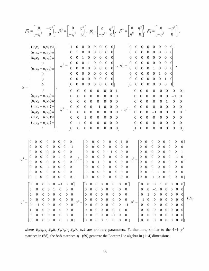
38

,0

04

5

2

,0

07

6

3

,0

06

7

3

,0

09

8

4

,0

08

9

4

,

)(

)(

)(

)(

)(

)(

0

0

0

0

)(

0

)(

)(

)(

1221

1331

2332

1441

2442

3443

4004

0330

2002

0110

s

wvuvu

wvuvu

wvuvu

wvuvu

wvuvu

wvuvu

wvuvu

wvuvu

wvuvu

wvuvu

S

,

00000001

00000000

00000000

00001000

00000000

00100000

01000000

00000000

,

00000000

00000010

00000100

00000000

00010000

00000000

00000000

10000000

,

10000000

01000000

00100000

00010000

00000000

00000000

00000000

00000000

,

00000000

00000000

00000000

00000000

00001000

00000100

00000010

00000001

32

10

,

00000100

00001000

00000000

00000000

01000000

10000000

00000000

00000000

,

00000000

00000001

00000000

00000100

00000000

00010000

00000000

01000000

,

00000010

00000000

00001000

00000000

00100000

00000000

10000000

00000000

654

.

00000000

00000000

00000000

00000000

00000001

00000010

00000100

00001000

,

00010000

00100000

01000000

10000000

00000000

00000000

00000000

00000000

,

00000000

00000000

00000001

00000010

00000000

00000000

00010000

00100000

987

(69)

where 43210 ,,,, uuuuu , swvvvvv ,,,,,, 43210 are arbitrary parameters. Furthermore, similar to the 4×4 i

matrices in (68), the 8×8 matrices i (69) generate the Lorentz Lie algebra in (1+4) dimensions.

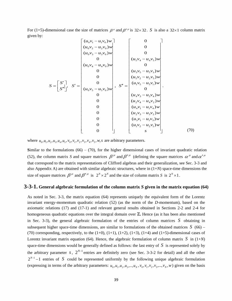
39

For (1+5)-dimensional case the size of matrices and is 3232 . S is also a 132 column matrix

given by:

.

)(

)(

)(

)(

)(

)(

0

)(

)(

)(

0

)(

0

0

0

,

0

0

0

0

0

0

0

)(

0

0

0

)(

0

)(

)(

)(

,

1221

3113

2332

4114

2442

4334

1551

5225

3553

5445

0550

0440

0330

0220

0110

s

wvuvu

wvuvu

wvuvu

wvuvu

wvuvu

wvuvu

wvuvu

wvuvu

wvuvu

wvuvu

Swvuvu

wvuvu

wvuvu

wvuvu

wvuvu

SS

SS

(70)

where 543210 ,,,,, uuuuuu , swvvvvvv ,,,,,,, 543210 are arbitrary parameters.

Similar to the formulations (66) – (70), for the higher dimensional cases of invariant quadratic relation

(52), the column matrix S and square matrices and

(defining the square matrices and

that correspond to the matrix representations of Clifford algebras and their generalization, see Sec. 3-3 and

also Appendix A) are obtained with similar algebraic structures, where in (1+N) space-time dimensions the

size of square matrices and

is

NN 22 and the size of column matrix S is 12 N.

3-3-1. General algebraic formulation of the column matrix S given in the matrix equation (64)

As noted in Sec. 3-3, the matrix equation (64) represents uniquely the equivalent form of the Lorentz

invariant energy-momentum quadratic relation (52) (as the norm of the D-momentum), based on the

axiomatic relations (17) and (17-1) and relevant general results obtained in Sections 2-2 and 2-4 for

homogeneous quadratic equations over the integral domain over ℤ. Hence (as it has been also mentioned

in Sec. 3-3), the general algebraic formulation of the entries of column matrices S obtaining in

subsequent higher space-time dimensions, are similar to formulations of the obtained matrices S (66) –

(70) corresponding, respectively, to the (1+0), (1+1), (1+2), (1+3), (1+4) and (1+5)-dimensional cases of

Lorentz invariant matrix equation (64). Hence, the algebraic formulation of column matrix S in (1+N)

space-time dimensions would be generally defined as follows: the last entry of S is represented solely by

the arbitrary parameter s , 12 N

entries are definitely zero (see Sec. 3-3-2 for detail) and all the other

12 1 N entries of S could be represented uniformly by the following unique algebraic formulation

(expressing in terms of the arbitrary parameters: Nuuuuu ,...,,,, 3210

, wvvvvv N ,,...,,,, 3210 ) given on the basis

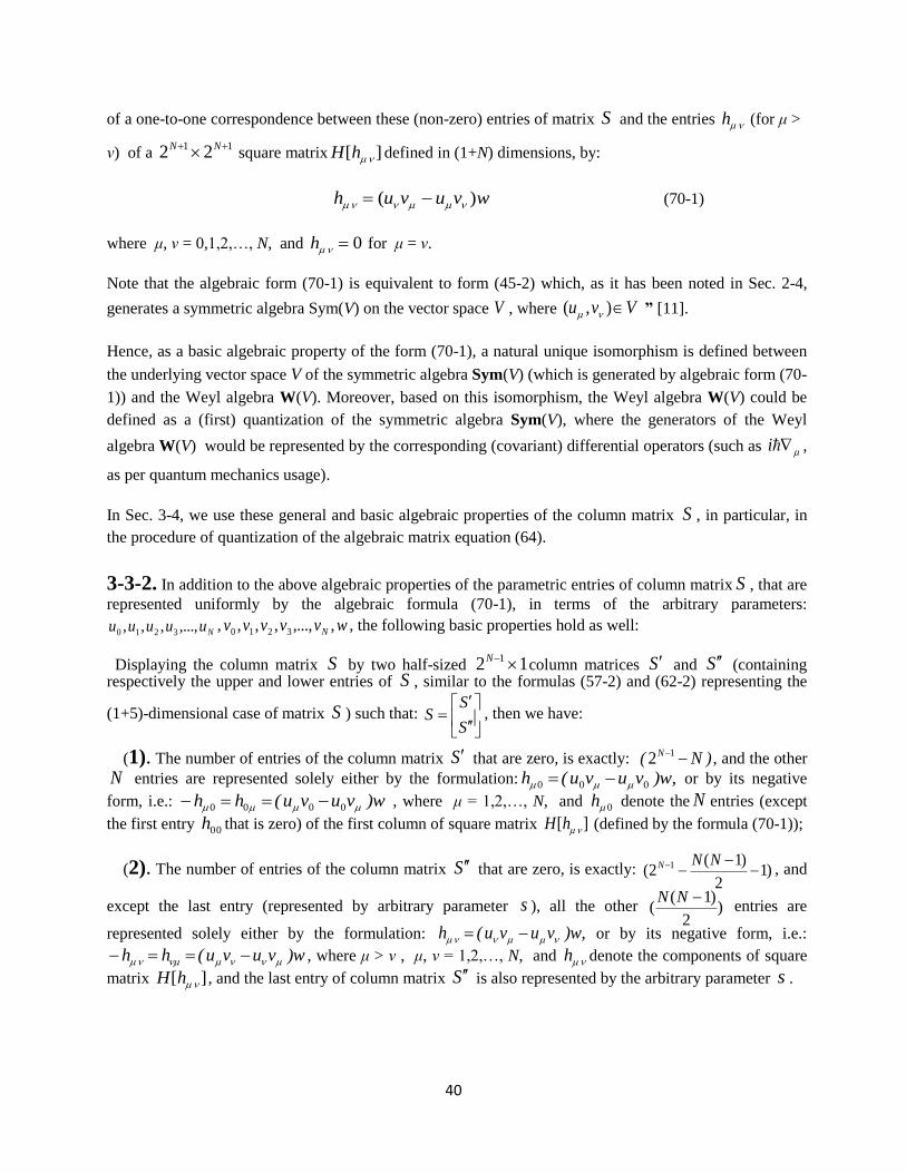
40

of a one-to-one correspondence between these (non-zero) entries of matrix S and the entries h (for μ >

ν) of a 11 22 NN square matrix ][ hH defined in (1+N) dimensions, by:

wvuvuh )( (70-1)

where μ, ν = 0,1,2,…, N, and 0h for μ = ν.

Note that the algebraic form (70-1) is equivalent to form (45-2) which, as it has been noted in Sec. 2-4,

generates a symmetric algebra Sym(V) on the vector space V , where Vvu ),( ” [11].

Hence, as a basic algebraic property of the form (70-1), a natural unique isomorphism is defined between

the underlying vector space V of the symmetric algebra Sym(V) (which is generated by algebraic form (70-

1)) and the Weyl algebra W(V). Moreover, based on this isomorphism, the Weyl algebra W(V) could be

defined as a (first) quantization of the symmetric algebra Sym(V), where the generators of the Weyl

algebra W(V) would be represented by the corresponding (covariant) differential operators (such as i ,

as per quantum mechanics usage).

In Sec. 3-4, we use these general and basic algebraic properties of the column matrix S , in particular, in

the procedure of quantization of the algebraic matrix equation (64).

3-3-2. In addition to the above algebraic properties of the parametric entries of column matrix S , that are

represented uniformly by the algebraic formula (70-1), in terms of the arbitrary parameters:

Nuuuuu ,...,,,, 3210, wvvvvv N ,,...,,,, 3210 , the following basic properties hold as well:

Displaying the column matrix S by two half-sized 12 1 Ncolumn matrices S and S (containing

respectively the upper and lower entries of S , similar to the formulas (57-2) and (62-2) representing the

(1+5)-dimensional case of matrix S ) such that:

S

SS , then we have:

(1). The number of entries of the column matrix S that are zero, is exactly: )N( N 12 , and the other

N entries are represented solely either by the formulation: ,w)vuvu(h 000 or by its negative

form, i.e.: w)vuvu(hh 0000 , where μ = 1,2,…, N, and 0h denote the N entries (except

the first entry 00h that is zero) of the first column of square matrix ][ hH (defined by the formula (70-1));

(2). The number of entries of the column matrix S that are zero, is exactly: )1

2

)1(2( 1

NNN , and

except the last entry (represented by arbitrary parameter s ), all the other )2

)1((

NN entries are

represented solely either by the formulation: ,w)vuvu(h or by its negative form, i.e.:

w)vuvu(hh , where μ > ν , μ, ν = 1,2,…, N, and h denote the components of square

matrix ][ hH , and the last entry of column matrix S is also represented by the arbitrary parameter s .

41

(3). If we exchange S and S in the column matrix

S

SS , that could be shown by,

S

S

S

S

I

IS

I

IS Ch

0

0

0

0)( (70-2)

then based on the general formulation of matrix S (defined uniquely by formulas (66) – (70) for various

space-time dimensions) and its algebraic properties (1) and (2) (mentioned above), it is concluded directly

that the matrix equation (64) given with the new column matrix )(ChS (70-2), i.e. equation:

0)~( )(

0 ChSkmp

, is which could be defined solely in (1+2) space-time dimensions for

0,0,0 11 vus , in (1+3) space-time dimensions for 0s , and in (1+4) space-time dimensions for

0,0,0 11 vus (which is reduced and be equivalent to the (1+3)-dimensional case of matrix

equation (64)). In (1+1) and (1+5) and higher space-time dimensions, the matrix equation

0)~( )(

0 ChSkmp

would be which are defined if and only if all the entries of column matrix

)(ChS are zero. This means that the matrix equation (64): 0)~( 0 Skmp

, is symmetric in the

exchange of S and S (in the column matrix

S

SS ), solely in (1+2)-dimensional space-time for

0,0,0 11 vus , and in (1+3)-dimensional space-time for 0s . In Sec. 3-5-2, this particular algebraic

property of the column matrix S would be used for concluding a new crucial and essential issue in

fundamental physics.

In the following Section, the natural isomorphism between the symmetric algebra Sym(V) (generated

uniquely by the algebraic form (70-1)) and the Weyl algebra W(V) mentioned in Sec. 3-3-1, in addition to

the general algebraic properties of column matrix S presented in Sec. 3-3-2, would be used and applied

directly in the procedure of first quantization of the Lorentz invariant system of linear equations (64).

3-4. A new unique mathematical derivation of the fundamental (massive) field

equations of physics (representing the laws governing the fundamental forces of nature):

By first quantization (followed by a basic procedure of minimal coupling to space-time geometry) of

the Lorentz invariant system of linear equation (64) (representing uniquely the equivalent form of

energy-momentum quadratic relation (52), see Sec. 3-3) expressed in terms of the Clifford algebraic

matrices (65) – (70),... , two classes of general covariant field equations are derived uniquely as

follows (given in (1+N) space-time dimensions):

0)~( )(

0 R

R kmi

, (71)

0)~( )(

0 F

F kmDi

(72)

where i and Di are the general relativistic forms of energy-momentum quantum operator

(where is the general covariant derivative, and D is gauge covariant derivative, for detail see the

ordinary tensor formalisms of these equations, representing by formulas (78-1) – (79-3), in Sec. 3-4-1),

42

)(

0

Rm and )(

0

Fm are the fields‘ invariant masses, )0,...,0,( 00gck is the general covariant

velocity in stationary reference frame (that is a time-like covariant vector), and

~ are two

contravariant NN 22 square matrices (compatible with the matrix representations of certain Clifford

algebras, see Sec. 3-3 and also Appendix A) defined by formulas (65) – (70) in Sec 3-3. In the field

equation (72), ΨR is a column matrix as a (first) quantized form of the algebraic column matrix S (defined by relations (64) – (70-1) in Sections 3-3, 3-3-1 and 3-3-2), determined and represented uniquely

by formulas (73) – (77),…, in various space-time dimensions. The column matrix ΨR contains the

components of field strength tensor R (equivalent to the Riemann curvature tensor), and also the

components of covariant quantity )(G

that defines the corresponding source current tensor by relation:

)()(

0)( )( RR

R kim

J

(which appears in the course of the derivation of field equation (71), see Sec.

3-4-2 for details). In a similar manner, in the tensor field equation (72), ΨF is also a column matrix as a

(first) quantized form of the algebraic column matrix S (defined by relations (64) – (70-1) in Sections 3-3,

3-3-1 and 3-3-2), determined and represented uniquely by formulas (73) – (77),…, in to various space-time

dimensions. The column matrix ΨF contains both the components of tensor field F (defined as the

gauge field strength tensor), and also the components of covariant quantity )(F that defines the

corresponding source current vector by relation: relation: )()(

0)( )( FF

F kim

DJ

(which appears in the

course of the derivation of field equation (72), see Sec. 3-4-2 for details). Moreover, the general covariance

formalism of the field equations (71) and (72), would be also shown in Sec. 3-4-1.

In addition, in Sec. 3-5, based on a basic class of discrete symmetries for the field equations (71) and (72),

along with definite mathematical axiomatic formalism of the derivation of these equations, it is shown that

these equations could be defined solely in (1+2) and (1+3) space-time dimensions. It is shown that (1+3)

dimensional cases of these equations represent uniquely a new formalism of bispinor fields of spin-2 and

spin-1 particles, respectively. It is also shown that the (1+2)-dimensional cases of these equations,

represent asymptotically new massive forms of bispinor fields of spin-3/2 and spin-1/2 particles,

respectively.

Moreover, in Sec. 3-5-2, based on the definite mathematical formalism of this axiomatic derivation

approach, the basic assumption (3) in Sec. 3-1, along with the C, P and T symmetries (represented

basically by their corresponding quantum matrix operators) of the fundamentally derived general

covariant field equations (71) and (72), it is concluded that the universe could be realized solely with the

(1+2) and (1+3)-dimensional space-times (where this conclusion, in particular, is based on the T-

symmetry). In Sections 3-5-3 and 3-5-4, it is proved that 'CPT' is the only (unique) combination of C, P,

and T symmetries that could be defined as a symmetry for interacting fields. In addition, in Sec. 3-5-4, on

the basis of these discrete symmetries of the field equations (71) and (72), it is shown that only left-

handed particle fields (along with their complementary right-handed fields) could be coupled to the

corresponding (any) source currents.

Furthermore, in Sec. 3-6, it is argued that the metric of background curved space-time is diagonalized for

the spin-1/2 fermion field equations (defined by the field equation (110) as a generalized form of (1+2)-

dimensional case of equation (72)), where this property generates a certain set of additional symmetries

corresponding uniquely to the SU(2)LU(2)R symmetry group for spin-1/2 fermion fields (represented by

43

two main groups of ―1+3‖ generations, corresponding respectively to two subgroups of leptons and two

subgroups of quarks), in addition to the SU(2)LU(2)R and SU(3) gauge symmetry groups for spin-1

boson fields coupled to the spin-1/2 fermionic source currents. Moreover, based on these uniquely

determined gauge symmetries, four new charge-less spin-1/2 fermions (representing by ―ze , zn ; zu , zd‖,

where two right-handed charhe-less quarks zu and zd emerge specifically in two subgroups with anti-

quarks such that: ( b,u,s , zu) and ( t,d,c , zd)), and also three new massive spin-1 bosons (representing

by ",~

,~

" ZWW

, where in particular Z

is the complementary right-handed particle of ordinary Z

boson), are predicted by this new mathematical axiomaticapproach.

As a particular result, in Sec. 3-4-2, based on the definite and unique formulation of the derived

Maxwell‗s equations (and also Yang-Mills equations, defined by the (1+3)-dimensional case of the field

equation (72), compatible with specific gauge symmetry groups as shown in Sec. 3-6-1-2 and 3-6-3-2), it

is also concluded that magnetic monopoles could not exist in nature.

3-4-1. Axiomatic Derivation of General Covariant Massive Field Equations (71) and (72):

First it should be noted that via first quantization (followed by a basic procedure of minimal coupling to

space-time geometry) of the algebraic systems of linear equations (64) (as a matrix equation given by the

Clifford algebraic matrices (65) – (70),…, in various space-time dimensions), two categories of general

covariant field equations (with a definite matrix formalism compatible with the Clifford algebras and their

generalizations, see Sec 3-3 and also Appendix A) are derived solely, representing by the tensor equations

(71) and (72) in terms two tensor fields R and ,F respectively. In fact, as it has been mentioned in

Sections 3-3-1 and 3-3-2, there is a natural isomorphism between the Weyl algebra and the symmetric

algebra generated by the algebraic form (70-1) which represents the general formulation of the entries of

algebraic column matrix S in the matrix equation (64). In addition, the procedure of minimal coupling to

space-time geometry would be simply defined as a procedure which, starting from a theory in flat space-

time, substitutes all partial derivatives by corresponding covariant derivatives and the flat space-time

metric by the curved space-time (pseudo-Riemannian) metric. Moreover, as mentioned in Sec. 3-3-1, on

the basis of this natural isomorphism, the Weyl algebra could be also represented as a quantization of the

symmetric algebra generated by the algebraic form (70-1)). Hence, using this natural isomorphism, by first

quantization (followed by a basic procedure of minimal coupling to space-time geometry) of matrix

equation (64), two definite classes of general covariant massive (tensor) field equations are determined

uniquely, expressed in terms of two basic connection forms (denoting by two derivatives and D

corresponding respectively to the diffeomorphism (or metric) invariance and gauge invariance), along with

their corresponding curvature forms, denoting respectively by R (as the gravitational field strength

tensor, equivalent to Riemann curvature tensor) and F (as the gauge field strength tensor). This natural

isomorphism could be represented by the following mappings (corresponding to the curvature formsR

and F , respectively):

RRwvuvu RR ),()( )( , (71-1)

μνFF Fig DDDDwvuvu )()( )( . (72-1)

44

where ),()(

R

ADADF , and Fg , A are respectively the

corresponding coupling constant and gauge field (that is defined generally as a Lie algebra-valued 1-form

representing by a unique vector field [58]). Based on this natural unique isomorphism represented by the

mappings (71-1) and (72-1), the column matrices ΨR and ΨF (in the expressions of field equations (71)

and (72), respectively) would be determined uniquely various dimensional space-times, represented by

formulas (73) – (77),… .

In addition, as mentioned in Sec. 3-4 in detail, the last entry of algebraic column matrix S in matrix

equation (64) (as it has been shown in the relations (64) – (70)), is represented by the arbitrary algebraic

parameter s . In the course of the derivation of field equations (71) and (72) (via the first quantization

procedure mentioned above, and the mappings (71-1) and (72-1)), the arbitrary parameter s could be

substituted solely by two covariant quantities )(R

and )(F that define the corresponding covariant

source currents )(R

and )(FJ (given in the field equations (71) and (72), respectively) by the conditional

relations: )()(

0)( )( RR

R kim

J

and )()(

0)( )( FF

F kim

DJ

.

In addition, as another basic issue concerning the general covariance formulation of tensor field equations

(71) and (72), we should note that each of these equations (as a system of equations) includes also an

equation corresponding to the 2nd

Bianchi identity, as follows, respectively:

0)()()()(

0

)(

0

)(

0 Rkim

Rkim

Rkim RRR

, (71-2)

0)()()()(

0

)(

0

)(

0 Fkim

DFkim

DFkim

DFFF

(72-2)

However, the tensor field R as the Riemann curvature tensor, obeys the relation (71-2) tensor, if and

only if a torsion tensor is defined in as: )()2( )(

0 kgkgimT R , and subsequently the

relation (71-2) be equivalent to the 2nd

Bianchi identity of the Riemann tensor. Consequently, the

covariant derivative should be also defined with this torsion, that we may show it by

. Moreover, as

it has been also shown in Sec. 3-4-2, concerning the relation (72-2), we may also define a torsion field as:

)()2( )(

0 kgkgimZ F , and write the relations (71-2) and (72-2) (representing the 2nd

Bianchi

identities) as follows:

,

RTRTRTRRR

(71-2-a)

0 FDFDFD

(72-2-a)

where the general relativistic form of gauge derivative D

has been defined with torsion field Z . We

use the derivatives

and D

in the ordinary tensor representations (i.e. the formulas (78-1) – (79-3))

of the field equations (71) and (72) in Sec. 3-4-2. In addition, based on the formulations of torsions T

and Z (that have appeared naturally in the course of derivation of the field equations (71) and (72))

and general properties of torsion tensors (in particular, this property that a torsion tensor can always be

45

treated as an independent tensor field, or equivalently, as part of the space-time geometry [72 - 74]), it

could be concluded directly that torsion field T generates the invariant mass of corresponding

gravitational field, and torsion field Z generates the invariant mass of corresponding gauge field,

respectively. Hence, based on our axiomatic derivation approach including the mappings (71-1) and (72-

1) (mentioned above), the (1+1), (1+2), (1+3), (1+4), (1+5),…, dimensional cases of column matrices ΨR

and ΨF in the specific expressions of general covariant massive (tensor) field equations (71) and (72), are

determined uniquely as follows, respectively; For (1+1)-dimensional space-time we have:

,

;)(

,)(,,

)()(

0)(

)()(

0)(

)(

10

)(

10

FF

F

RR

R

FFRR

kim

DJ

kim

JFR

(73)

- For (1+2)-dimensional space-time we obtain:

;)(

,)(,,

)()(

0)(

)()(

0)(

)(

21

02

10

)(

21

02

10

FF

F

RR

R

F

F

R

R

kim

DJ

kim

J

F

F

F

R

R

R

(74)

- For (1+3)-dimensional space-time we have:

;)(

,)(,

0,

0

)()(

0)(

)()(

0)(

)(

12

31

23

30

20

10

)(

12

31

23

30

20

10

FF

F

RR

R

F

F

R

R

kim

DJ

kim

J

F

F

F

F

F

F

R

R

R

R

R

R

(75)

- For (1+4)-dimensional space-time we get,

;)(

,)(,

0

0

0

0

0

,0

0

0

0

0

)()(

0)(

)()(

0)(

)(

21

31

32

41

42

43

04

30

02

10

)(

21

31

32

41

42

43

04

30

02

10

FF

F

RR

R

F

F

R

R

kim

DJ

kim

J

F

F

F

F

F

F

F

F

F

F

R

R

R

R

R

R

R

R

R

R

(76)

46

- For (1+5)-dimensional space-time we obtain:

)()(

0)(

)()(

0)(

)(

21

13

32

14

42

34

51

25

53

45

50

40

30

20

10

)(

21

13

32

14

42

34

51

25

53

45

50

40

30

20

10

)(

,)(,

0

0

0

0

0

0

0

0

0

0

0

0

0

0

0

0

,

0

0

0

0

0

0

0

0

0

0

0

0

0

0

0

0

FF

F

RR

R

F

F

R

R

kim

DJ

kim

J

F

F

F

F

F

F

F

F

F

F

F

F

F

F

F

R

R

R

R

R

R

R

R

R

R

R

R

R

R

R

(77)

where in the relations (73) – (77), )(RJ and )(FJ are the source currents expressed, necessarily, in terms of

the covariant quantities

)(G

and )(F (as the initially given quantities), respectively. For higher-

47

dimensional space-times, the column matrices R and F (with similar formulations) are determined

uniquely as well.

3-4-2. From the field equations (71) and (72) (derived uniquely with certain matrix formalisms

compatible with the Clifford and Weyl algebras), the following general covariant field equations, with

ordinary tensor formalisms, are obtained (but not vice versa), respectively:

,

RTRTRTRRR

(78-1)

)()(

0 )( RR JRkimR

; (78-2)

),()(

R

)()(

0)( )( RR

R kim

J

, ).(

2

)(

0 kgkg

imT

R

(78-3)

and

,0 FDFDFD

(79-1)

)(FJFD

; (79-2)

ADADF

,

)()(

0)( )( FF

F kim

DJ

, ).(

2

)(

0 kgkg

imZ

F

(79-3)

where is the affine connection:

K ,

is the Christoffel symbol (or the torsion-

free connection), K is the contorsion tensor defined by: kgimK R )2( )(

0 (that is anti-

symmetric in the first and last indices), T is the torsion given by: KKT (that generates

the invariant mass of the gravitational field), )0,...,0,( 00gck (where we supposed 1c ) is the

covariant velocity of particle (or the static observer) in the stationary reference frame, and A is the gauge potential vector field. Moreover, in general covariant field equations (79-1) – (79-3), the covariant

derivative D

has been defined specifically with the torsion field Z (generating the invariant mass of

gauge field strength tensor F ).

It should be emphasized again that the tensor field equations (78-1) – (78-3) and (79-1) – (79-3) (which

are obtained respectively from the original equations (71) and (72), but not vice versa) show merely the

general covariance formalism (including torsions fields T and

Z ) of the axiomatically derived field

equations (71) and (72). The crucial issue here is that the original field equations (71) and (72) could not

be obtained from the tensor equations (78-1) – (78-3) and (79-1) – (79-3). In fact, the tensor equations

(78-1) – (78-3) and (79-1) – (79-3) don’t represent completely the definite matrix formalism (compatible

with certain Clifford and Weyl algebras) of the axiomatic field equations (71) and (72). Hence, based on

this mathematical axiomatic formalism and derivation approach of equations (71) and (72) (presented in

Sections 3-3 – 3-4-1), it is concluded that the fundamental force fields of physics cannot be described

completely via the ordinary tensor representations of these fields (in the current standard classic and

quantum relativistic field theoretic formalism of physics), such as the representations (78-1) – (78-3) and

48

(79-1) – (79-3); and as shown in Sections 3-3 – 3-4-1, on the basis of this new mathematical formalism,

all the fundamental force fields of physics could be represented (and described) solely by the

axiomatically determined and formulated field equations (71) and (72) with their definite covariant matrix

formalisms (given and specified by formulas (65) – (70) for various space-time dimensions, compatible

with certain Clifford and Weyl algebras).

3-4-2-1. Derivation of the Einstein field Equations

Along with the massive gravitational field equations (78-1) – (78-3) (obtained uniquely from the

originally derived field equations (71)) that are expressed solely in terms of R as the field strength

tensor and also torsion‘s depended terms, we also assume the following relation as basic definition for the

Ricci tensor (where the Riemann curvature tensor and Ricci tensor don‘t obey the interchange

symmetries: RR , RR , because of the torsion [28]):

Rkim

Rkim

Rkim RRR

)()()()(

0

)(

0

)(

0

(78-4)

where the relation (78-4) particularly remains unchanged by the transformation:

gRR (78-5)

(where as would be shown, is equivalent to the cosmological constant). It should be noted that by

taking 0 , from the 2nd

Bianchi identity of the Riemann curvature tensor and relation (78-4) it could

be shown that the Ricci tensor is also the contraction of the Riemann tensor, i.e. RR (which is

equivalent to the ordinary definition of the Ricci tensor). However, this ordinary definition for the Ricci

tensor, necessarily, doesn‘t imply the above transformation. In fact, in the following, we show that this

basic transformation is necessary for having the cosmological constant in the gravitational field equations

(including the Einstein field equations which could be derived from the above equations and relations)

expressed in terms of the Ricci and stress-energy tensors. As a direct result, a unique equivalent

expression of gravitational field equations, in terms of the Ricci tensor R and stress-energy tensor T ,

could be also determined from the basic definition (78-4) (for Ricci curvature tensor, based on this

axiomatic formalism), and field equations (78-1) – (78-3), along with the following expression for current )(RJ (defined in terms of the stress-energy tensor T , )(

TT , and metric g , in D-dimensional

space-time):

])()[(8])()[(8)(

0

)(

0

)(

0

)(

0)(

Tgkim

Tgkim

BTkim

Tkim

JRRRR

R

, (78-6)

where TT for 0)(

0 Rm , 0B for 2,1D , and )2/(1 DB for 3D . , the Einstein field

equations (as the massless case) are determined directly as follows:

gBTgTR )(8 (78-7)

3-4-3. Showing that magnetic monopoles could not exist in nature. As a direct consequence of the

uniquely derived general covariant field equations (72) that are specified by the matrices (73) – (77) and

(65) – (70) (or the general covariant field equations (79-1) – (79-3) obtained from the original equation

49

(72)), which , in fact, represent the electromagnetic fields equivalent to a generalized massive form of the

Maxwell‘s equations (as well as a generalized massive form of the Yang-Mills fields corresponding to

certain gauge symmetry groups, see Sec. 3-6), it is concluded straightforwardly that magnetic

monopoles could not exist in nature.

3-4-4. On the local gauge invariance of uniquely derived new general covariant massive (matrix)

forms of the Maxwell’s (and Yang-Mills) and Dirac equations.

The Lagrangian density specified for the tensor field F in the field equations (79-1) – (79-3) is

(supposing 0)( FJ )[58]:

FFgL F *)( )41( (80)

where g is the metric's determinant. Moreover, the trace part of torsion field Z in (79-3) is obtained as:

kNk)im(NZZ )F( 20

(81)

where (1+N) is the number of space-time dimensions and 2

)(

0

Fim . Now based on the definition of

covariant vector k (as a time-like covariant vector), we simply get: k: . This basic property,

along with and formula (81), imply the general covariant massive field equations (79-1) – (79-3)

(formulated originally with the torsion field (79-3) generating the invariant mass )(

0

Fm of field F ), and

the corresponding Lagrangian density (80), be invariant under the U(1) Abelian gauge group [9, 58, 60-

63]. However, in Sec. 3-6, we show that assuming the spin-1/2 fermion fields (describing generally by the

field equation (110-9) compatible with specific gauge symmetry group (110-12), as shown in Sec. 3-6-1-

2) and their compositions as the source currents of the (1+3)-dimensional cases of general covariant

massive field equation (72) (describing the spin-1 boson field), then this field equation would be invariant

under two types of gauge symmetry groups, including: SU(2)LU(2)R and SU(3), corresponding with a

group of seven bosons and a groups of eight bosons (as shown in Sec. 3-6-3-2).

3-4-5. Identifying a new particular massive gauge boson.

According to Refs. [60 – 63], in agreement with the recent astronomical data, we can directly establish a

lower bound for a constant quantity which is equivalent to the constant 2

)(

0

Fim (defined by the

relation (80)) as: 21 . Hence, a new massive particle (corresponding to the U(1) symmetry group)

would be identified with the invariant mass:

m ≈ 4.90571×10-50

kg (82)

that is generated by a coupling torsion field of the type (79-3) of the background curved space-time.

In addition, it should be noted that, in general, based on the covariant massive field equations (71) and

(72) derived by our axiomatic approach (or field equations (78-1) – (78-3) and (79-1) – (79-3) obtained

from (71) and (72)), the invariant masses of the elementary particles are generated by torsion fields of the

types (78-3) (for spin-3/2 and spin-2 particles) and (79-3) (for spin-1/2 and spin-1 particles, see Sec. 3-6).

50

Hence, this approach could be also applied for massive neutrinos concluding that their masses are

generated by the coupling torsion fields (of the type (79-3)). Such massive particle fields coupled to the

torsions (of the type (79-3)) of the background space-time geometry could be completely responsible for

the mysteries of dark energy and dark matter [75].

3-5. Quantum Representations of C, P and T Symmetries of the Axiomatically Derived

General Covariant Massive (tensor) Field Equations (71) and (72):

As it has been shown in Sections 3-3, 3-3-1, 3-3-2, 3-4 and 3-4-1, the general covariant massive

(tensor) field equations (71) and (72) as the unique axiomatically determined equations (representing

the fundamental field of physics, as assumed in Sec. 3-1), are represented originally with definite

matrix formalisms constructed from the combination of two specific matrix classes including the

column matrices (73) – (77),… compatible with the Weyl algebras (based on the isomorphism (71-1)

– (72-1)), and the square matrices (65) – (70),… that are compatible with the Clifford algebras and

their generalizations; see Sections 3-3, 3-3-1, 3-3-2 and 3-4-1 and also Appendix A for detail).

In agreement with the principles of relativistic quantum theory [35], and also as another primary

assumption in addition to the basic assumption (3) defined in Sec. 3-1, we basically represent the C,

P and T symmetries of the source-free cases of by the following quantum matrix operators (with the

same forms in both flat and curved space-time), respectively:

(Note: In Sec. 3-5-3, we show that only a certain simultaneous combination of the C, P and T

transformations could be defined for the field equations (71) and (72) with non-zero source currents.)

(1)- Parity Symmetry (P-Symmetry):

I

IP P

0

0 (83)

where I is the identity matrix, and the size of matrix

P in (1+N)-dimensional space-time is NN 22 .

The operator P obeys the relations:

TPPPPPP ˆˆˆˆ,1ˆ,1)ˆdet( 12

(83-1)

(2)- Time-Reversal Symmetry (T-Symmetry):

KiKTT ChP 0 (84)

where the operator K denotes complex conjugation, the operator P defined by formula (83) and the

operator Ch

in (1+1) and (1+2) space-time dimensions, is given by:

,

I

ICh

0

0 (84-1)

and in (1+3) and higher space-time dimensions, Ch is denoted by:

0

0

iI

iICh (84-2)

51

where the size of matrix Ch in (1+N)-dimensional space-time is:

NN 22 . Moreover, in (1+1) and (1+2)

space-time dimensions, the time reversal operator T (84) and the Hermitian operator ChPiT 0

ˆ

(specified in the formula (84)) obey the relations:

,ˆˆˆˆ,1ˆ

00

1

00

2 TTTTTT

(84-3)

and in (1+3) and higher space-time dimensions, T and 0T obey the relations:

T

TTTTT 00

1

00

2 ˆˆˆˆ,1ˆ

(84-4)

Concerning the time reversal symmetry, it should be noted that the relations (84-3) are solely compatible

with the fermionic fields, and relations (84-4) are solely compatible with the bosonic fields. In addition, it

should be noted that these basic quantum mechanical properties (i.e. the relations (84-3) and (84-4)) of the

time reversal symmetry (84), are fully compatible with corresponding properties of the field tensors F

and R presented in Sec. 3-6, where the tensor field F (describing by general covariant field

equation (72)) represents (asymptotically) solely a massive bispinor field of spin-1/2 particles (as a

new general covariant massive formulation of the Dirac equation) in (1+2) space-time dimensions,

and also represents a massive bispinor field of spin-1 – as new massive general covariant (matrix)

formulations of both Maxwell and Yang-Mills field equations compatible with specified gauge

symmetry groups – in (1+3) space-time dimensions; and tensor field R (describing by general

covariant field equation (71)) represents (asymptotically) solely a bispinor field of spin-3/2 particles

(as a new massive general covariant form of the Rarita–Schwinger equation) in (1+2) space-time

dimensions , and also represents a massive bispinor field spin-2 particles (equivalent to a generalized

massive form of the Einstein equations) in (1+3) space-time dimensions.

(3)- Charge Conjugation Symmetry (C-Symmetry):

FFCFRRCR KiICKiIC ˆ~)(,ˆ~

)( (85)

where KiIC ˆ~ , I is the identity matrix, the operator K denotes complex conjugation, and the charge

conjugation operator C defined by: T)(ˆ)( RCR C , T)(ˆ)( FCF C . The charge conjugation operator

C obeys the following relations:

TCCCCCC ˆˆˆˆ,1ˆˆ 1

(85-1)

As a basic additional issue, it is worth to note that the time-reversal operator (84) could be also expressed

basically in terms of the parity matrix operator P (83), matrix operator KiIC ˆ~

given in the definition

of charge-conjugated transformation (85), and matrix Ch defined by formulas (84-1) and (84-2), as

follows:

TCChP ˆ~

(85-2)

where we have: PChChP .

3-5-1. Basic Properties of Matrix (operator) Ch (defined by formulas (84-1) and (84-2)):

52

In this Section, the main properties of matrix operator Ch

(defined by unitary matrices (84-1) and

(84-2)) hav been presented. Each of general covariant (tensor) field equations (71) and (72) (including

their source-free and non source-free cases), as a system of differential equations, is symmetric and

has the same spectrum by multiplying by matrixCh . The multiplied column matrices

R

ChCh

R )(

and

F

ChCh

F )( then obey the equations (71) and (72), respectively, but with opposite sign in

mass term such that: 0)~( )()(

0 Ch

R

R kmi

, 0)~( )()(

0 Ch

F

F kmi

.

As a general additional issue concerning the column matrices R

ChCh

R )( and F

ChCh

F )(,

should be also added that the sign change of the mass terms introduced in the field equations (71) and

(72) is immaterial (the same property also hold for the ordinary formulation of Dirac equation, and so

on [32]). In other words, the field equations (71) of the form 0)~( )(

0 R

R kmi

are

equivalent, and similarly the field equations (72) of the form 0)~( )(

0 F

F kmi

would be

equivalent as well. However, since the algebraic column matrix S in the matrix equation (64)

(derived and represented uniquely in terms of the matrices (66) – (70),… corresponding to various

space-time dimensions), is not symmetric by multiplying by matrixCh (84-1) and (84-2) (except for

(1+2) and (1+3)-dimensional cases of column matrix S , based on the definite algebraic properties of

matrix S presented in Sections 3-3, 3-3-1, 3-3-2), it is concluded that except the (1+2) and (1+3)-

dimensional cases of the fundamental field equations (71) and (72), these field equations could not be

defined with the column matrices of the types )()(

R

ChCh

R and )()(

F

ChCh

F (if assuming

that the column matrices R and

F are defined with field equations (71) and (72), i.e. they have

the formulations similar to the formulations of originally derived column matrices (73) – (77),…

corresponding to various space-time dimensions). This conclusion follows from this fact that the

filed equations (71) and (72) have been derived (and defined) uniquely from the matrix equation (64)

via the axiomatic derivation approach (including the first quantization procedure) presented in

Sections 3-4, 3-4-1. In Sec. 3-5-2, using this property (i.e. multiplication of column matrices R and

F defined in the fundamental field equations (71) and (72), by matrix Ch (84-1) and (84-2) from

the left), this crucial and essential issue would be concluded directly that by assuming the time-

reversal invariance of the general covariant filed equations (71) and (72) (represented by the

transformations RTˆ and

FTˆ , where the quantum operator T is given uniquely by formula (84),

i.e.: KiKTT ChP ˆˆˆˆ0 ), these fundamental field equations could be defined solely in (1+2) and

(1+3) space-time dimensions (with the column matrices of the forms (96-1) and (98-2), respectively).

Subsequently, in Sec. 3-5-3, , it would be also shown that only a definite simultaneous combination

of all the transformations ,C P , T and also matrix Ch (given by quantum operators (83) – (87))

could be defined for the field equations (71) and (72) with non-zero source currents. In addition, the

matrix operator Ch in (1+1) and (1+2) space-time dimensions obeys the relations:

TChChChChCh )()()(,1)( 12

, (86)

and in the (1+3) and higher dimensions obeys the following relations as well:

53

TChChChChCh )()()(,1)( 12

(87)

Furthermore, in Sec. 3-5-4, the matrix Ch would be also used basically for defining and representing

the left-handed and right handed components of the column field matrices R and F defined

originally in the field equations (71) and (72).

3-5-2. Showing that the universe could be realized solely with the (1+2) and (1+3)-dimensional

space-times:

The proof of this essential property of nature within the new mathematical axiomatic formalism presented

in this article, is mainly based on the T-symmetry (represented basically by quantum matrix operators

(84)) of the fundamentally derive general covariant field equations (71) and (72). As shown in Sec. 3-5,

the source-free cases (as basic cases) of field equations (71) and (72) are invariant under the time-reversal

transformation defined by matrix operator (84). Moreover, in Sec. 3-5-3, it would be also shown that

these field equations with non-zero source currents are solely invariant under the simultaneous

transformations of all the ,C P , and T (83) – (85), multiplied by matrix Ch (given by formulas

(84-1) and (84-2)). Now, following the definite mathematical formalism of the axiomatic derivation

approach of fundamental field equations (71) and (72), assuming that any column matrixRX , or

FY ,

expressible in the tensor formulation of general covariant field equation (71) or (72), is basically

definable, if and only if, it could be also derived originally as a column matrix via the axiomatic

derivation approach presented in Sections 3-4 and 3-4-1.

On this basis, it could be shown that the time-reversal transformed forms of the column matrices R

and

F given in the expressions of source-free cases of field equations (71) and (72), are definable

solely in (1+2) and (1+3)-dimensional space-times. Based on this result, along with the basic

assumption (3) in Sec. 3-1, it is concluded directly that the universe could be realized solely with the

(1+2) and (1+3)-dimensional space-times. We show this in the following in detail.

As noted, in fact, the above conclusion follows directly from the formulations of uniquely determined

time-reversal transformed forms of column matrices R

and

F given in the expressions of source-

free cases of field equations (71) and (72). Denoting these column matrices by RR T ˆЖ

and

FF T ˆЖ , where the time-reversal operator (84) is defined by: KiKTT ChP 0 , they would be

determined as follows in various dimensions:

- For (1+1)-dimensional space-time we have:

;),(

0),(ˆ),(ˆ),(Ж,

),(

0),(ˆ),(ˆ),(Ж

10

0

10

0

tiFtTtTt

tiRtTtTt FFFRRR

xxxx

xxxx

(88)

- For (1+2)-dimensional space-time it is obtained:

54

;0

Ж0

Ж

02

10

21

0

02

10

21

0

)t,(iF

)t,(iF

)t,(iF

)t,(T)t,(T)t,(,

)t,(iR

)t,(iR

)t,(iR

)t,(T)t,(T)t,( FFFRRR

x

x

x

xxx

x

x

x

xxx

(89)

- For (1+3)-dimensional space-time we get:

;

0

0Ж

0

0Ж

30

20

10

12

31

23

0

30

20

10

12

31

23

0

)t,(iF

)t,(iF

)t,(iF

)t,(iF

)t,(iF

)t,(iF

)t,(T)t,(T)t,(,

)t,(iR

)t,(iR

)t,(iR

)t,(iR

)t,(iR

)t,(iR

)t,(T)t,(T)t,( FFFRRR

x

x

x

x

x

x

xxx

x

x

x

x

x

x

xxx

(90)

- For (1+4)-dimensional space-time we have:

;

0

0

0

0

0

0

Ж

0

0

0

0

0

0

Ж

04

30

02

10

21

31

32

41

42

43

0

04

30

02

10

21

31

32

41

42

43

0

)t,(iF

)t,(iF

)t,(iF

)t,(iF

)t,(iF

)t,(iF

)t,(iF

)t,(iF

)t,(iF

)t,(iF

)t,(T)t,(T)t,(,

)t,(iR

)t,(iR

)t,(iR

)t,(iR

)t,(iR

)t,(iR

)t,(iR

)t,(iR

)t,(iR

)t,(iR

)t,(T)t,(T)t,( FFFRRR

x

x

x

x

x

x

x

x

x

x

xxx

x

x

x

x

x

x

x

x

x

x

xxx

(91)

55

- For (1+5)-dimensional space-time we obtain:

;

0

00

0

0

0

0

0

0

0

0

0

0

0

0

0

0

Ж

0

00

0

0

0

0

0

0

0

0

0

0

0

0

0

0

Ж

50

40

30

20

10

21

13

32

14

42

34

51

25

53

45

0

50

40

30

20

10

21

13

32

14

42

34

51

25

53

45

0

)t,(iF

)t,(iF

)t,(iF

)t,(iF

)t,(iF

)t,(iF

)t,(iF

)t,(iF

)t,(iF

)t,(iF

)t,(iF

)t,(iF

)t,(iF

)t,(iF

)t,(iF

)t,(T)t,(T)t,(,

)t,(iR

)t,(iR

)t,(iR

)t,(iR

)t,(iR

)t,(iR

)t,(iR

)t,(iR

)t,(iR

)t,(iR

)t,(iR

)t,(iR

)t,(iR

)t,(iR

)t,(iR

)t,(T)t,(T)t,( FFFRRR

x

x

x

x

x

x

x

x

x

x

x

x

x

x

x

xxx

x

x

x

x

x

x

x

x

x

x

x

x

x

x

x

xxx

(92)

Now based on the formulations of the derived time-reversal transformed column matrices RЖ and FЖ

(88) – (92), although they could be expressed merely in the tensor formulations of field equations (71)

and (72), however, except the (1+2) and (1+3)-dimensional cases of these transformed column matrices,

56

all the other cases cannot be derived originally as a column matrix via the axiomatic derivation approach

presented in Sections 3-4 and 3-4-1 (following the formulation of originally derived column matrices (73)

– (77)). Below this conclusion (and subsequent remarkable results) is discussed in more detail.

**********************************

In addition, it is also worth to note that on the basis of our derivation approach, since there are not the

corresponding isomorphism (that could be represented by the unique mappings (71-1) and (72-1), in Sec.

3-4-1) between the entries of column matrices RЖ and FЖ (88), (91), (92),… and the entries (with the

exactly same indices) of column matrix S (in the algebraic matrix equation (64), where its last entry, i.e.

arbitrary parameter ―s‖ is zero compatible with the source-free cases of the field equations (71) and

(72)) that are given uniquely as follows in (1+1) and (1+4), (1+5),... and higher space-time dimensions,

respectively, using the definitions (66) – (70),… (in Sec. 3-3), and also the algebraic properties of

column matrix S (presented in Sections 3-3-1 and 3-3-2) representing in terms of two half-sized 12 1 N

column matrices S and S such that:

S

SS (where

Nuuuuu ,...,,,, 3210, wvvvvv N ,,...,,,, 3210 are arbitrary

parameters):

- For (1+1)-dimensional space-time we have:

0

)( 0110 wvuvu

S

SS ; (93)

- For (1+4), (1+5)-dimensional space-times we get, respectively:

;

0

)(

)(

)(

)(

)(

)(

0

0

0

0

)(

0

)(

)(

)(

,

1221

1331

2332

1441

2442

3443

4004

0330

2002

0110

wvuvu

wvuvu

wvuvu

wvuvu

wvuvu

wvuvu

S

wvuvu

wvuvu

wvuvu

wvuvu

S

S

SS

,;

0

)(

)(

)(

)(

)(

)(

0

)(

)(

)(

0

)(

0

0

0

,

0

0

0

0

0

0

0

)(

0

0

0

)(

0

)(

)(

)(

,

1221

3113

2332

4114

2442

4334

1551

5225

3553

5445

0550

0440

0330

0220

0110

...

wvuvu

wvuvu

wvuvu

wvuvu

wvuvu

wvuvu

wvuvu

wvuvu

wvuvu

wvuvu

Swvuvu

wvuvu

wvuvu

wvuvu

wvuvu

SS

SS

(94)

it would be directly concluded that in (1+1) and (1+4), (1+5),... and higher space-time dimensions, the

column matrices RЖ and FЖ could not be defined as the column matrices in unique formulations of the

axiomatically derived general covariant field equations (71) and (72). In other words, for the (1+2)-

dimensional cases of the transformed column matrices RЖ and

FЖ (89), the corresponding isomorphism

(represented uniquely by the mappings (71-1) and (72-1)) could be defined between the components of

57

these matrices and the entries of column matrix S (67), for s = 0 (compatible with ,0)( R

0)( F ), if

and only if: 0),(02 tiR xand 0),(02 tiF x . This could be shown as follows:

.0),(,0),(

,0

),(

),(

0

),(

Ж,

),(

),(

0

),(

Ж

0

)(

)(

)(

0202

2002

02

10

21

02

10

21

1221

2002

0110

tiFtiR

vuvu

tiF

tiF

tiF

tiR

tiR

tiR

wvuvu

wvuvu

wvuvu

S FR

on)Quantizati (FirstProcedure Derivation

xx

x

x

x

x

x

x

(95)

where for appeared parametric condition: ,02002 vuvu as it would be shown in Sec. 3-5-2-1, it could

be supposed solely: 0022 , uvvu , implying conditions: 002 R and 002 F , which could be

assumed for the field strength tensors R and F in (1+2)-dimensional space-time (without vanishing

these tensor fields), based on their basic definitions given by formulas (71-1) and (72-1).

Hence, definite mathematical framework of our axiomatic derivation approach (presented in Sec. 3-4), in

addition to the time-reversal invariance (represented by the quantum operator (84)) of source-free cases of

general covariant field equations (71) and (72), imply the (1+2)-dimensional case of column matrices ΨR

and ΨF given by relations (74) (where we assumed ,0)( R

0)( F ), could be given solely as follows,

to be compatible with the above assumed conditions (i.e. being compatible with the mathematical

framework of axiomatic derivation of field equations (71) and (72), and also the time-reversal invariance

defined by quantum operator (84)), and consequently, as the column matrices could be defined in the

formulations of the fundamental tensor field equations (71) and (72), respectively:

0

0,

0

0

21

10

21

10

F

F

R

R

FR

(96)

The formulations (96) that are represented the column matrices ΨR and ΨF in the field equations (71) and

(72) compatible with the above basic conditions, are also represented these matrices in the field equations

(71) and (72) with non-zero source currents compatible with two basic conditions (similar to above

conditions) including a unique combination of the C, P and T symmetries (that have been represented by

quantum operators (83) – (85)) for these cases of field equations (71) and (72), and also the mathematical

framework of axiomatic derivation of equations (71) and (72). In fact, as it has been shown in Sec. 3-5-1,

the field equations (71) and (72) with non-zero source currents could have solely a certain combination

(given by formulas (86) and (87)) of the C, P and T symmetries (that are represented by the operators

(83), (84) and (85)). This unique combined symmetry in addition to the unique formulations (96) of

source-free cases of column matrices ΨR and ΨF in (1+2)-dimensional space-time, implies these matrices

could take solely the following forms to be defined in the formulations of the fundamental tensor field

equations (71) and (72) (with non-zero source currents):

58

)()(

0)(

)()(

0)(

)(

21

10

)(

21

10

)(

,)(,

0,

0

FF

F

RR

R

F

F

R

R

kim

DJ

kim

J

F

F

R

R

(96-1)

In the same manner, concerning the (1+4)-dimensional cases of column matrices RЖ and

FЖ (91), there

would be a mapping between the entries of these matrices and entries (with the same indices) of algebraic

column matrix S (69), where s = 0 (compatible with ,0)( R

0)( F ), if and only if: ,0),(10 tiR x

,0),(41 tiR x ,0),(31 tiR x 0),(21 tiR x, ,0),(10 tiF x ,0),(41 tiF x ,0),(31 tiF x ,0),(21 tiF x i.e.:

.0),(,0),(

,0),(,0),(

,0),(,0),(

,0),(,0),(

,0,0

0

0

0

),(

0

),(

),(

),(

0

),(

),(

),(

),(

),(

),(

0

Ж,

0

0

0

),(

0

),(

),(

),(

0

),(

),(

),(

),(

),(

),(

0

Ж

0

)(

)(

)(

)(

)(

)(

0

0

0

0

)(

0

)(

)(

)(

4141

3131

2121

1010

11

04

30

02

10

21

31

32

41

42

43

04

30

02

10

21

31

32

41

42

43

1221

1331

2332

1441

2442

3443

4004

0330

2002

0110

tiFtiR

tiFtiR

tiFtiR

tiFtiR

vu

tiF

tiF

tiF

tiF

tiF

tiF

tiF

tiF

tiF

tiF

tiR

tiR

tiR

tiR

tiR

tiR

tiR

tiR

tiR

tiR

wvuvu

wvuvu

wvuvu

wvuvu

wvuvu

wvuvu

wvuvu

wvuvu

wvuvu

wvuvu

S FR

on)Quantizati (FirstProcedure Derivation

xx

xx

xx

xx

x

x

x

x

x

x

x

x

x

x

x

x

x

x

x

x

x

x

x

x

(97)

This means that in (1+4) space-time dimensions, the mathematical framework of our axiomatic derivation

approach (described in Sec. 3-4) in addition to the time reversal invariance (defined by the quantum

operator (84)) of the source-free case of the derived general covariant fundamental field equations (71)

and (72) imply the column matrices ΨR and ΨF (76) (for ,0)( R

0)( F ) could take solely the

following forms (in general) to be defined in the formulations of the field equations (71) and (72):

59

0

0

0

0

0

0

0

0

0

0

,

0

0

0

0

0

0

0

0

0

0

32

42

43

04

30

02

32

42

43

04

30

02

F

F

F

F

F

F

R

R

R

R

R

R

FR

(98)

which are equivalent to the (1+3)-dimensional source-free cases of column matrices ΨR and ΨF

(represented uniquely by formulas (75))

In addition, similar to the formulations (96-1), as it has been shown in Sec. 3-5-1, the field equations (71)

and (72) with non-zero source currents have a certain (and unique) combination of the C, P and T

symmetries (that have been defined by the operators (83), (84) and (85)). This combined symmetry in

addition to the forms (98), imply also the (1+4)-dimensional cases of column matrices ΨR and ΨF

represented by formula (76) could take solely the following forms (in general) to be defined in the

formulations of fundamental field equations (71) and (72):

)()(

0)(

)()(

0)(

)(

32

42

43

04

30

02

)(

32

42

43

04

30

02

)(

,)(,

0

0

0

0

0

0

0

0

0

,

0

0

0

0

0

0

0

0

0

FF

F

RR

R

F

F

R

R

kim

DJ

kim

J

F

F

F

F

F

F

R

R

R

R

R

R

(98-1)

60

Consequently, the (1+4)-dimensional cases of column matrices ΨR and ΨF that are originally given by

formulations (76), are reduced to formulas (98-1) which are equivalent to the (1+3)-dimensional cases of

these matrices (given originally by column matrices of the forms (75)), i.e.:

.)(

,)(,

0,

0

)()(

0)(

)()(

0)(

)(

12

31

23

30

20

10

)(

12

31

23

30

20

10

FF

F

RR

R

F

F

R

R

kim

DJ

kim

J

F

F

F

F

F

F

R

R

R

R

R

R

(98-2)

Moreover, as it would be also noted in Sec. 3-6, it is noteworthy to add that the tensor field R in

column matrix ΨR (98-2) (expressing the general representation of column matrices definable in the

formulation of (1+3)-dimensional case of general covariant field equation (71)), in fact, equivalently

represents a massive bispinor field of spin-2 particles in (1+3) space-time dimensions (which could be

identified as a definite generalized massive matrix formulation of the Einstein gravitational field, as it has

been also shown in Sec. 3-4-2), and the tensor field F in the column matrix ΨF (98-2) (expressing the

general representation of column matrices definable in the formulation of (1+3)-dimensional case of

general covariant field equation (72)), in fact, equivalently represents a massive bispinor field of spin-1

particles in (1+3) space-time dimensions (which could be identified as definite generalized massive

formulation of the Maxwell electromagnetic field, as it has been also shown in Sections 3-4-2 and 3-4-4;

and also Yang-Mills fields compatible with specific gauge groups, as it would be shown in Sec. 3-6).

Summing up, in this Section (Sec. 3-5-2) we showed that the axiomatic approach of derivation of the

field equations (71) and (72) (described in Sections 3-1, 3-3 and 3-4) in addition to their time reversal

invariance (represented basically by the quantum operator (84)), imply these fundamentally derived

equations could be solely defined in (1+2) and (1+3) space-time dimensions. ―Hence, based on the

later conclusion and also the basic assumption (3) (defined in Sec. 3-1), we may conclude

directly that the universe could be realized solely with the (1+2) and (1+3)-dimensional

space-times, and cannot have more than four space-time dimensions.‖

Based on the axiomatic arguments and relevant results presented and obtained in this Section, in the

following Sections we consider solely the (1+2) and (1+3)-dimensional cases of general covariant field

equations (71) and (72) that are defined solely with the column matrices of the forms (96-1) and (98-2).

3-5-2-1. Equivalent (asymptotically) representations of the bispinor fields of spin-3/2 and

spin-1/2 particles, respectively, by general covariant field equations (71) and (72) (formulated

solely with column matrices of the types (96-1)) in (1+2) space-time dimensions:

It is noteworthy that according to the Ref. [29] and also based on the basic properties of the Riemann

curvature tensor R in (1+2) space-time dimensions [64] (in particular the identity:

61

GR , where

G is the Einstein tensor and ), it would be concluded that R which is

defined by (1+2)-dimensional case of the general covariant massive field equation (71) (which could be

defined solely with a column matrix of the type ΨR (96-1)), represents asymptotically a general

covariant bispinor field of spin-3/2 particles (that would be asymptotically equivalent to the Rarita–

Schwinger equation). In a similar manner, according to the Ref. [29], and also following the basic

properties of field strength tensor F in (1+2) space-time dimensions (that as a rank two anti-symmetric

with three independent components holding, in particular, the identities:

TF ,

FT )21( ,

showing that F could be represented equivalently by a vector T with three independent components as

well) it would be concluded that F which is defined by (1+2)-dimensional case of the general

covariant massive (tensor) field equation (72) (which could be defined solely with a column matrix of the

type ΨF (96-1)), represents asymptotically a general covariant bispinor field of spin-1/2 particles (that

would be asymptotically equivalent to the Dirac equation [29]). Furthermore, as it would be shown in

Sec. 3-6, the general covariant field equations (72) (representing asymptotically the spin-1/2 fermion

fields) is also compatible with the SU(2)LU(2)R symmetry group (representing ―1+3‖ generations for

both lepton and quark fields including a new charge-less fermion).

3-5-2-2. Equivalent representations of the bispinor fields of spin-2 and spin-1 particles,

respectively, by general covariant field equations (71) and (72) (defined solely with column

matrices of the types (98-2)) in (1+3) space-time dimensions:

It should be also note that according to the Refs. [31 – 36], the basic properties of the Riemann curvature

tensor including the relevant results presented in Sec. 3-4-2 , it would be concluded that the field strength

tensor R (i.e. the Riemann tensor) the in (1+3) space-time dimensions by general covariant

massive (tensor) field equation (71) (formulated solely with a column matrix of the type ΨR (98-2)),

represents a general covariant bispinor field of spin-2 particles (as a generalized massive formulation

of the Einstein gravitational field equation). In a similar manner, according to the Refs. [31 – 36], the

field strength tensor F which is defined in (1+3) space-time dimensions by the general covariant

massive (tensor) field equation (72) (formulated solely with a column matrix of the type ΨF (98-2)),

represents a general covariant bispinor field of spin-1 particles (representing new generalized

massive formulations of the Maxwell‘s equations, and also Yang-Mills field equations). Furthermore,

as it would be shown in Sec. 3-6, the general covariant field equations (72) (representing the spin-1

boson fields coupling to the spin-1/2 fermionic currents) is also compatible with the SU(2)LU(2)R

and SU(3) symmetry groups.

Moreover, based on these determined gauge symmetries for the derived fermion and boson field

equations, four new charge-less spin-1/2 fermions (representing by ―ze , zn ; zu , zd‖, where two right-

handed charhe-less quarks zu and zd emerge specifically in two subgroups with anti-quarks such that:

( b,u,s , zu) and ( t,d,c , zd)), and also three new massive spin-1 bosons (representing by

",~

,~

" ZWW

, where in particular Z

is the complementary right-handed particle of ordinary Z

boson), are predicted uniquely by this new mathematical axiomatic approach.

62

3-5-3. Showing that only a definite simultaneous combination of the quantum mechanical

transformations C , P , T and Ch

(given uniquely by the matrix operators (83) – (87)) could be

defined for the general covariant massive (tensor) field equations (71) and (72) with non-zero

source currents:

As it has been shown in Sections 3-5-1 and 3-5-2, since the algebraic column matrix S in the matrix

equation (64) (derived and represented uniquely in terms of the matrices (66) – (70),…

corresponding to various space-time dimensions), is not symmetric by multiplying by matrixCh (84-

1) and (84-2) (except for (1+2) and (1+3)-dimensional cases of column matrix S , based on the

definite algebraic properties of matrix S presented in Sections 3-3, 3-3-1, 3-3-2), it is concluded that

except the (1+2) and (1+3)-dimensional cases of the fundamental field equations (71) and (72), these

field equations could not be defined with column matrices of the type )()(

R

ChCh

R

and

)()(

F

ChCh

F (if assuming that the column matrices R and

F are defined with field equations

(71) and (72), i.e. they have the formulations similar to the formulations of originally derived column

matrices (73) – (77),… corresponding to various space-time dimensions). This conclusion follows

from this fact that the filed equations (71) and (72) have been derived (and defined) uniquely from

the matrix equation (64) via the axiomatic derivation approach (including the first quantization

procedure) presented in Sections 3-4, 3-4-1. As it has been shown in Sec. 3-5-2, using this property

(i.e. multiplication of column matrices R and

F , defined in the unique expressions of

fundamental field equations (71) and (72), by matrix Ch from the left), this crucial and essential

issue is concluded directly that by assuming the time-reversal invariance of the general covariant

filed equations (71) and (72) (represented by the transformations RTˆ and

FTˆ , where the

quantum operator T is given uniquely by formula (84), i.e.: KiKTT ChP ˆˆˆˆ0 ), these

fundamental field equations could be defined solely in (1+2) and (1+3) space-time dimensions (with

the column matrices of the forms (96-1) and (98-2), respectively).

Hence, the definite mathematical formalism of the axiomatic approach of derivation of fundamental

field equations (71) and (72), along with the C, P and T symmetries (represented by the quantum matrix

operators (83) – (87), in Sec. 3-5) of source-free cases (as basic cases) of these equations, in fact, imply

these equations with non-zero source currents, would be invariant solely under the simultaneous

combination of all the transformations ,C P , and T (83) – (85), multiplied by matrix Ch (defined

by formulas (84-1) and (84-2)). This unique combined transformation could be expressed uniquely as

follows, respectively, for the particle fields (representing by column matrices ),( trR

, ),( trF

)

and their corresponding antiparticle fields (representing by column matrices ),( trR

, ),( trF

given

solely with reversed signs of the temporal and spatial coordinates):

);,( ˆˆˆ),(ˆ

),,( ˆˆˆ),(ˆ

trCPTtrZ

trCPTtrZ

F

Ch

F

R

Ch

R

COMB

COMB

(99)

63

).,( ˆˆˆ),(

~

),,( ˆˆˆ),(~

trCPTtrZ

trCPTtrZ

F

Ch

F

R

Ch

R

COMB

COMB

(100)

The unique combined form of transformation COMB

Z (99) (and also COMB

Z~

(100), where COMBCOMB

ZZ ˆ~ ) is

based on the following two basic issues:

Firstly, it follows from the definite formulations of uniquely determined column matrices (73) – (77),… (corresponding to various space-time dimensions, however, as noted above, based on the arguments presented in Sec. 3-5-2, the only definable column matrices in the formulations of field equations (71) and (72), are of the types ΨR and ΨF represented by formulas (96-1) and (98-2), in (1+2)

and (1+3) space-time dimensions, respectively), where the source currents )(RJ and

)(FJ should be

expressible by these conditional relations (in terms of the arbitrary covariant quantities )(R

and )(F ),

respectively: )(

)(

0)( )( RR

R kim

J

, )(

)(

0)( )( FF

F kim

J

. In other words, the unique formulation

of derived combined symmetries COMB

Z and COMB

Z~

represented by the quantum operatorsCOMB

Z (99) and

COMBZ~

(100), in particular, is a direct consequent of the above conditional expressions for source currents

)(RJ and )(FJ . As noted in Sec. 3-4-1, these relations appear as necessary conditions in the course of

the axiomatic derivation of general covariant field equations (71) and (72). In fact, in the field equations (71) and (72) the uniquely derived column matrices ΨR and ΨF (73) – (77),…, not only contain all the

components of tensor fields ρσμνR and μνF , but also contain the components of arbitrary covariant

quantities )(R

and )(F (as the initially given quantities) which define the source currents

)(RJ and

)(FJ by the above expressions, respectively, i.e.: )(

)(

0)( )( RR

R kim

J

, )(

)(

0)( )( FF

F kim

J

.

Now based on these conditional expressions in addition to this natural and basic circumstance that the

source currents)(RJ and

)(FJ should be also transferred respectively as a rank three tensor and a vector,

under the parity, time-reversal and charge conjugation transformations (defined by formulas (83) – (85)) of the field equations (71) and (72), it would be concluded directly that the transformations (99) and

(100) are the only simultaneous combinations of transformations ,C P , T (also including the matrix Ch , necessarily, as it would be shown in the following paragraph), which could be defined for the

field equations (71) and (72) with ―non-zero‖ source currents.

Secondly, appearing the matrix operator Ch in simultaneous combinations ˆˆˆ CPTCh and ˆˆˆ CPTCh

in the combined transformations (99) and (100), follows simply from the basic arguments presented in

Sec. 3-5-2. In fact, in these uniquely determined combinations, the simultaneous multiplication by matrix

Ch (from the left) is a necessary condition for that the transformed column matrices: ),(ˆ trZ RCOMB

,

),(~

trZ RCOMB

, ),(ˆ trZ FCOMB

, ),(

~trZ FCOMB

(given in the transformations (99) and (100)) could be

also defined in the field equations (71) and (72), based on the formulations of column matrices (96-1) and

(98-2), as mentioned in Sec. 3-5-2) (however, it is worth to note that this argument is not merely limited

to the definability of column matrices of the types (96-1) and (98-2), and it could be also represented on

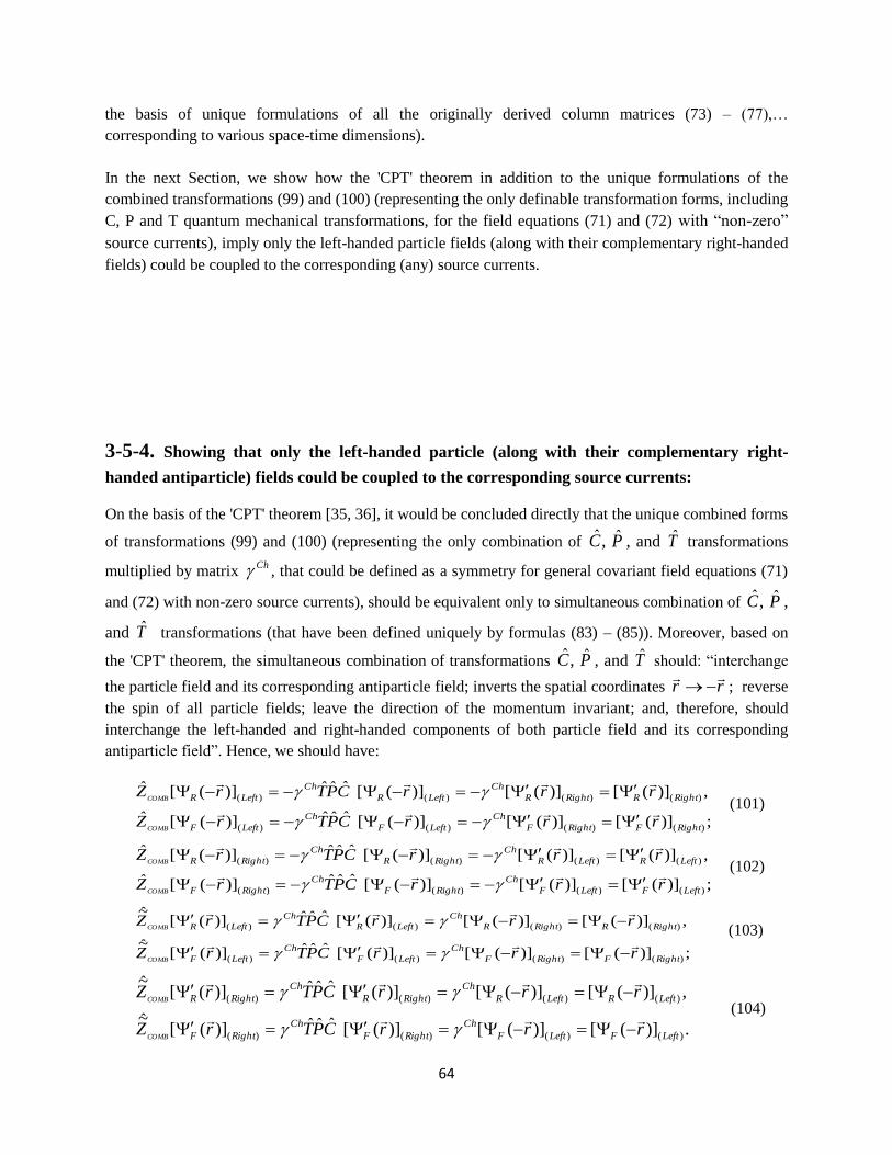
64

the basis of unique formulations of all the originally derived column matrices (73) – (77),…

corresponding to various space-time dimensions).

In the next Section, we show how the 'CPT' theorem in addition to the unique formulations of the

combined transformations (99) and (100) (representing the only definable transformation forms, including

C, P and T quantum mechanical transformations, for the field equations (71) and (72) with ―non-zero‖

source currents), imply only the left-handed particle fields (along with their complementary right-handed

fields) could be coupled to the corresponding (any) source currents.

3-5-4. Showing that only the left-handed particle (along with their complementary right-

handed antiparticle) fields could be coupled to the corresponding source currents:

On the basis of the 'CPT' theorem [35, 36], it would be concluded directly that the unique combined forms

of transformations (99) and (100) (representing the only combination of ,C P , and T transformations

multiplied by matrix Ch , that could be defined as a symmetry for general covariant field equations (71)

and (72) with non-zero source currents), should be equivalent only to simultaneous combination of ,C P ,

and T transformations (that have been defined uniquely by formulas (83) – (85)). Moreover, based on

the 'CPT' theorem, the simultaneous combination of transformations ,C P , and T should: ―interchange

the particle field and its corresponding antiparticle field; inverts the spatial coordinates rr

; reverse

the spin of all particle fields; leave the direction of the momentum invariant; and, therefore, should

interchange the left-handed and right-handed components of both particle field and its corresponding

antiparticle field‖. Hence, we should have:

;)]([)]([)]([ ˆˆˆ)]([ˆ

,)]([)]([)]([ ˆˆˆ)]([ˆ

)()()()(

)()()()(

RightFRightF

Ch

LeftF

Ch

LeftF

RightRRightR

Ch

LeftR

Ch

LeftR

rrrCPTrZ

rrrCPTrZ

COMB

COMB

(101)

;)]([)]([)]([ ˆˆˆ)]([ˆ

,)]([)]([)]([ ˆˆˆ)]([ˆ

)()()()(

)()()()(

LeftFLeftF

Ch

RightF

Ch

RightF

LeftRLeftR

Ch

RightR

Ch

RightR

rrrCPTrZ

rrrCPTrZ

COMB

COMB

(102)

;)]([)]([)]([ ˆˆˆ)]([

~

,)]([)]([)]([ ˆˆˆ)]([~

)()()()(

)()()()(

RightFRightF

Ch

LeftF

Ch

LeftF

RightRRightR

Ch

LeftR

Ch

LeftR

rrrCPTrZ

rrrCPTrZ

COMB

COMB

(103)

.)]([)]([)]([ ˆˆˆ)]([

~

,)]([)]([)]([ ˆˆˆ)]([~

)()()()(

)()()()(

LeftFLeftF

Ch

RightF

Ch

RightF

LeftRLeftR

Ch

RightR

Ch

RightR

rrrCPTrZ

rrrCPTrZ

COMB

COMB

(104)

65

where the column matrices )( rR

and )( rF

represent the particle field and )(rR

and )(rF

denote the transformed forms of column matrices of )( rR

and )( rF

, respectively, under the

simultaneous combination of transformations ,C P , and T (83) – (85). Furthermore, in agreement and

based on the definitions and properties of quantum operators C , P , T and matrix Ch given by

formulas (83) – (87), the left-handed and right-handed components of column matrices of the types (96-

1) and (98-2) (representing the unique formulations of column matrices that could be defined in the field

equations (71) and (72), as mentioned in Sec. 3-5-2) are defined solely as follows for the column matrices

)( rR

, )( rF

and also )(rR

, )(rF

(as the transformed forms of column matrices )( rR

and

)( rF

under the TPC ˆˆˆ transformation, respectively):

)],()([

2

1)]([

)],()([2

1)]([

)(

)(

rγrr

rγrr

F

Ch

FLeftF

R

Ch

RLeftR

)];()([2

1)]([

)],()([2

1)]([

)(

)(

rγrr

rγrr

F

Ch

FRightF

R

Ch

RRightR

(105)

)],()([2

1)]([

)],()([2

1)]([

)(

)(

rγrr

rγrr

F

Ch

FLeftF

R

Ch

RLeftR

)].()([2

1)]([

)],()([2

1)]([

)(

)(

rγrr

rγrr

F

Ch

FRightF

R

Ch

RRightR

(106)

where we have:

,)]([)]([)(

,)]([)]([)(

)()(

)()(

RightFLeftFF

RightRLeftRR

rrr

rrr

.)]([)]([)(

,)]([)]([)(

)()(

)()(

RightFLeftFF

RightRLeftRR

rrr

rrr

(107)

Now using the definitions (105) and (106) in the formulas (101) – (104), we obtain:

;)]([)]()([

2

1)]()([

2

1)]([

,)]([)]()([2

1)]()([

2

1)]([

)()(

)()(

LeftFFF

Ch

F

Ch

F

Ch

LeftF

Ch

LeftRRR

Ch

R

Ch

R

Ch

LeftR

Ch

rrrγrγrr

rrrγrγrr

(101-1)

;)]([)]()([

2

1)]()([

2

1)]([

,)]([)]()([2

1)]()([

2

1)]([

)()(

)()(

RightFFF

Ch

F

Ch

F

Ch

RightF

Ch

RightRRR

Ch

R

Ch

R

Ch

RightR

Ch

rrrγrγrr

rrrγrγrr

(102-1)

;)]([)]()([

2

1)]()([

2

1)]([

,)]([)]()([2

1)]()([

2

1)]([

)()(

)()(

LeftFFF

Ch

F

Ch

F

Ch

LeftF

Ch

LeftRRR

Ch

R

Ch

R

Ch

LeftR

Ch

rrrγrγrr

rrrγrγrr

(103-1)

.)]([)]()([2

1)]()([

2

1)]([

,)]([)]()([2

1)]()([

2

1)]([

)()(

)()(

RightFFF

Ch

F

Ch

F

Ch

RightF

Ch

RightRRR

Ch

R

Ch

R

Ch

RightR

Ch

rrrγrγrr

rrrγrγrr

(104-1)

66

Based on the relations (101-1) – (104-1), it would be concluded directly that only the left-handed

components of particle fields representing by )()]([ LeftR r

, )()]([ LeftF r

, and the right-handed

components of their corresponding antiparticle fields representing by )()]([ RightR r

, )()]([ RightF r

(as the

transformed forms of column matrices )()]([ LeftR r

and )()]([ LeftF r

under the TPC ˆˆˆ transformation,

respectively), obey the transformations (101-1) and (104-1) (as the necessary conditions given

respectively by relations (101) and (104)). On the other hand, the right-handed components of particle

fields representing by )()]([ RightR r

, )()]([ RightF r

, and the left-handed components of their

corresponding antiparticle fields representing by )()]([ LeftR r

, )()]([ LeftF r

(as the transformed forms of

column matrices )()]([ RightR r

and )()]([ RightF r

under the TPC ˆˆˆ transformation, respectively), don‘t

obey the transformations (102-1) and (103-1) (as the necessary conditions given respectively by relations

(102) and (103)). Hence (and also following the basic assumption (3) defined in Sec. 3-1), it is

concluded directly that only the left-handed particle fields (along with their complementary

right-handed fields) could be coupled to the corresponding (any) source currents. This means

that only left-handed bosonic fields (along with their complementary right-handed fields) could

be coupled to the corresponding fermionic source currents; which also means that only left-

handed fermions (along with their complementary right-handed fermions) can participate in any

interaction with the bosons (which consequently would be only left-handed bosons or their

complementary right-handed bosons).

3-6. Showing the gauge invariance of axiomatically derived general covariant (tensor) field

equation (72) in (1+2)-dimensional space-time (definable with column matrices of the type ΨF (96-

1), representing the spin-1/2 fermion fields) under the SU(2)LU(2)R symmetry group, and also

invariance of this equation in (1+3)-dimensional space-time (definable column matrices of the type

ΨF (98-2), representing the spin-1 boson fields coupled to the fermionic source currents) under the

SU(2)LU(2)R and SU(3) symmetry group:

One of the natural and basic properties of the (1+2)-dimensional space-time geometry is that the metric

tensor can be ―diagonalized‖ [78]. Using this basic property, the invariant energy-momentum quadratic

relation (52) (in Sec. 3-1-1) would be expressed as follows:

0)()()()( 2

2

222

1

112

0

002

0

00 pgpgpgpg st (108)

that is equivalent to: 2

0

2

2

222

1

112

0

00 )()()()( cmpgpgpg , where (as defined in Sec. 3-1-1) 0m and p

are the particle‘s rest mass and momentum (3-momentum), μ

st

μ kmp 0 , and )0,0,()0,0,( 00

0 gckk μ

denotes the covariant form of the 3-velocity of particle in stationary reference frame. As it would be shown in the following, a crucial and essential property of the quadratic relation (108) is its invariance

under a certain set of sign inversions of the components of particle‘s momentum: ),,( 210 ppp , along with

similar inversions for the components:

),,( 210

ststst ppp , where000 kmpst , 021 stst pp . This set includes

seven different types of the sign inversions (in total), which could be represented simply by the following symmetric group of transformations (based on the formalism of the corresponding Lorentz symmetry group of invariant relation (108)), respectively:

67

),,,(),,,(),,,( )1(

2

)1(

1

)1(

0

)1(

021002100 pppppppppppp ststst (108-1)

),,,(),,,(),,,( )2(

2

)2(

1

)2(

0

)2(

021002100 pppppppppppp ststst (108-2)

),,,(),,,(),,,( )3(

2

)3(

1

)3(

0

)3(

021002100 pppppppppppp ststst (108-3)

),,,(),,,(),,,( )4(

2

)4(

1

)4(

0

)4(

021002100 pppppppppppp ststst (108-4)

),,,(),,,(),,,( )5(

2

)5(

1

)5(

0

)5(

021002100 pppppppppppp ststst (108-5)

),,,(),,,(),,,( )6(

2

)6(

1

)6(

0

)6(

021002100 pppppppppppp ststst (108-6)

),,,(),,,(),,,( )7(

2

)7(

1

)7(

0

)7(

021002100 pppppppppppp ststst (108-7)

Moreover, although, following noncomplex- algebraic values of momentum‘s components p )( pp ,

the corresponding complex representations of transformations (108-1) – (108-7) is not a necessary issue in general, however, if the invariant relation (108) is represented formally by equivalent complex form:

0)()()()( 22

22

11

11

00

00

00

00 ppgppgppgppg stst , (108-8)

then, along with the set seven real-valued transformations (108-1) – (108-7), this relation would be also

invariant under these corresponding sets of complex transformations (for 7,...,3,2,1a ):

),,,(),,,( )(

2

)(

1

)(

0

)(

02100

aaastast ipipipippppp , ),,,(),,,( )(

2

)(

1

)(

0

)(

02100

aaastast ipipipippppp

(108-9)

In Sec. 3-6-1-1, using the transformations (108-1) – (108-7) (along with their corresponding complex

forms (108-9)), a certain set of seven simultaneous (different) general covariant field equations

(corresponding to a group of seven bispinor fields of spin-1/2 particles) would be determined as particular

cases of the (1+2)-dimensional form of general covariant field equation (72) (defined with a column

matrix of the type (96-1)).

3-6-1. Following the definite formulation of (1+2)-dimensional case of system of linear equation (64)

(formulated in terms of the matrices (67)), for the energy-momentum relation (108) (along with the

transformations (108-1) – (108-7)), the following set of seven systems of linear equations (with different

parametric formalisms) is determined uniquely. The general parametric solution of each of these systems

of linear equations, obeys also the quadratic relation (108) (representing a set of seven forms, with

different parametric formulations, of the general parametric solutions of quadratic relation (108)). This set

of the seven systems of linear equations could be represented uniformly by a matrix equation as follows:

0)~( )()(

0

)( aaa Skmp

(109)

where 7,...,3,2,1a , kmp aast )(

0

)( , and

~ are two contravariant 44 real matrices (compatible

with matrix representations of the Clifford algebra Cℓ1,2) defined solely by formulas (65) and (67), and

parametric column matrix )(aS is also given uniquely as follows (formulated on the basis of definite

parametric formulation of column matrix S (67) in (1+2) space-time dimensions):

s

wvuvu

wvuvu

wvuvu

Saaaa

aaaa

aaaa

a

)(

)(

)(

)(

1

)(

2

)(

2

)(

1

)(

2

)(

0

)(

0

)(

2

)(

0

)(

1

)(

1

)(

0

)( (109-1)

68

which includes seven cases with specific parametric formulations expressed respectively in terms of

seven groups of independent arbitrary parameters: )(

2

)(

1

)(

0

)(

2

)(

1

)(

0 ,,,,, aaaaaa vvvuuu , and two common arbitrary

parameters s and w (i.e. having the same forms in all of the seven cases of column matrix )(aS ). In

addition, concerning the specific parametric expression (109-1) of column matrix )(aS in the formulation

of matrix equation (109), it is necessary to add that this parametric expression has been determined

specifically by assuming (as a basic assumption in addition to the systematic natural approach of

formulating the matrix equation (109), based on the definite formulation of axiomatically determined

matrix equation (64)) the minimum value for total number of the arbitrary parameters in all of seven cases

of column matrix )(aS , which implies equivalently the minimum value for total number of the arbitrary

parameters in all of seven simultaneous (different) cases of matrix equation (109) (necessarily with seven

independent parametric solutions representing a certain set of seven different equivalent forms of the

general parametric solution of quadratic relation (108), based on the general conditions of basic definition

of the systems of linear equations corresponding to homogeneous quadratic and higher degree equations,

presented in Sec. 2, and Sections 2-2 – 2-4, 3-1-1 concerning the homogenous quadratic equations).

In the following, in the derivation of the corresponding field equations (from matrix equation (109)), we

will also use the above particular algebraic property of parameters s which has been expressed

commonly in the expressions of all of seven simultaneous cases of matrix equation (109) (and also in Sec.

3-6-2, concerning the (1+3)-dimensional corresponding form of matrix equation (109), which holds the

similar property).

3-6-1-1. In addition, along with the transformations (108-1) – (108-7) and algebraic matrix equation

(109), using the corresponding complex transformations (108-9), we may also formally have the

following equivalent matrix equation (with the complex expression):

0)~( )()(

0

)( aaa Skimpi

(109-2)

where 7,...,3,2,1a , and kmp aast )(

0

)( . Although, based on the real value of momentum )(

p

)( )()( aa pp , the complex expression of each of the seven cases of algebraic matrix equation (109),

definitely, is not a necessary issue at the present stage. However, since the corresponding momentum

operator )(ˆ ap has a complex value (where

)()( ˆˆ aa pp ), in the following, using this basic property of the

momentum operator, we derive a certain set of seven different simultaneous general covariant field

equations from the matrix equations (109) and (109-2) (based on the general axiomatic approach of

derivation of general covariant massive field equation (72), presented in Sections 3-4 – 3-4-5, in addition

to certain forms of quantum representations of the C, P and T symmetries of this field equation, presented

in Sections 3-5 – 3-5-4). Furthermore, in Sec. 3-6-1-2, it would be also shown that the uniform

representation of this determined set of seven simultaneous field equations, describe a certain group of

seven simultaneous bispinor fields of spin-1/2 particles (corresponding, respectively, to a new right-

handed charge-less fermion in addition to three right-handed anti-fermions, along with their three

complementary left-handed fermions).

Furthermore, concerning the gravitational field equation (71), it should be noted that following from the

fact that the general covariant field equation (71) should describe, uniquely and uniformly, the

background space-time geometry via a certain form of the Riemann curvature tensor (which should be

determined from the tensor field equation (71)), the matrix equation (109) could not be used for the

derivation of a set of simultaneous different spin-3/2 fermion fields in (1+2) dimensions (there would be

the same condition for the field equation (71) in higher-dimensional space-times).

69

Hence, based on the axiomatic approach of derivation of (1+2)-dimensional case of field equation (72)

(defined solely by a column matrix of the form (96-1) in (1+2) space-time dimensions, as shown in Sec.

3-5-2), from the matrix equation (109) and (109-2) (defined solely by column matrix (109-1)), and also

taking into account the momentum operator‘s property: pp ˆˆ , the following group of seven

simultaneous (different) general covariant field equations could be determined:

0)~( )()(

0

)( f

F

ff kmDi

(110)

specifying by the following group of transformations (based on the corresponding group of

transformations (108-1) – (108-7) and (108-9)), for 7,...,3,2,1f , respectively

),,,(),,,( 2100

)1(

2

)1(

1

)1(

0

)1(

0 DDmDDDmD (110-1)

),,,(),,,( 2100

)2(

2

)2(

1

)2(

0

)2(

0 DDmDDDmD (110-2)

),,,(),,,( 2100

)3(

2

)3(

1

)3(

0

)3(

0 DDmDDDmD (110-3)

),,,(),,,( 2100

)4(

2

)4(

1

)4(

0

)4(

0

iDiDimiDDDmD (110-4)

),,,(),,,( 2100

)5(

2

)5(

1

)5(

0

)5(

0

iDiDimiDDDmD (110-5)

),,,(),,,( 2100

)6(

2

)6(

1

)6(

0

)6(

0

iDiDimiDDDmD (110-60

),,,(),,,( 2100

)7(

2

)7(

1

)7(

0

)7(

0

iDiDimiDDDmD (110-7)

where the column matrix

)( f

F would be also given as follows (based on the definite formulation of

column matrix F (96-1) in Sec. 3-5-2, expressing the general representation of column matrices

definable in the formulation of (1+2)-dimensional case of general covariant field equation (72)):

F

fff

F

f

f

f

F kim

DJF

F

)(,0 )(

0)()(

)(

21

)(

10

)(

(110-8)

where in all of the seven simultaneous cases of field equation (110) defined respectively by the column

matrices )( f

F (110-8) (for 7,...,3,2,1f ), the scalar quantity F (that as a given initial quantity,

defines the source currents )( fJ

(110-8)), necessarily, has the same value, based on the definite

parametric formulation of the algebraic column matrix (109-1) (in particular, the common form of the

corresponding arbitrary parameter s in the expressions of all of the seven simultaneous cases of matrix

equation (109)).

3-6-1-2. Following the definite formulations of set of seven general covariant (massive) field equations

(110) (specified, respectively, by the group of seven transformations (110-1) – (110-7)), the set of these

could be represented uniformly by the following general covariant field equation as well (defined solely

in (1+2) space-time dimensions):

0)~( 0 FkmDi

(110-9)

70

where the column matrix F given by:

F

F

F kim

DJF

F

)(,0

0

21

10

(110-10)

and the field strength tensor F , scalar F

, along with the source current J are defined as follows:

7

1

)(

f

f

fFF ,

.)()(7

1

)(7

1

)(

0)(02 JJk

imDk

imDI

f

f

f

f

F

ff

F

(110-11)

where I is the 22 identity matrix, and 2

f

f

l (for 7,...,3,2,1f ) are a set of seven 22

complex

matrices given by,

2

f

f

l ,

765

4

321

,,

,

,,,

lll

l

lll

1

0

0

1,

0

0,

0

1

1

0

,10

01

,0

0,

0

1

1

0,

0

0

i

i

i

i

i

i

(110-12)

which as would be shown in the following, represents uniformly a combined gauge symmetry group of

the form: SU(2)LU(2)R , where the sub-set of three matrices ― 321 ,, ‖ corresponds to SU(2)L group,

and subset of four matrices ― 7654 ,,, ‖ corresponds to U(2)R group.

Now based on the matrix formulation of field strength tensor F (defined by the general covariant field

equation (110-9)), and on the basis of C, P and T symmetries of this field equation (as a particular form

of the (1+2)-dimensional case of field equation (72)) that have been represented basically by their

corresponding quantum operators (in Sections 3-5 – 3-5-4), it would be concluded that the general

covariant field equation (110-9) describes uniformly a group of seven spin-1/2 fermion fields

corresponding to, respectively: ―three left-handed fermions (for 3,2,1f ), in addition to their three

complementary right-handed anti-fermions (for 7,6,5f ), and also a new single charge-less right-

handed spin-1/2 fermion (for 4f )‖. Hence, following the basic algebraic properties of seven matrices

f (110-12), and the gauge symmetry group of the type: SU(2)LU(2)R generated by these matrices, the

three matrices 321 ,,

(corresponding with SU(2)L) represent respectively ―three left-handed

fermions‖, and four matrices 7654 ,,, (corresponding with U(2)R) represent respectively: ―a new

single right-handed charge-less spin-1/2 fermion, and three right-handed spin-1/2 fermions as the

complementary particles of the three left-handed spin-1/2 fermions represented by matrices 321 ,, ‖ .

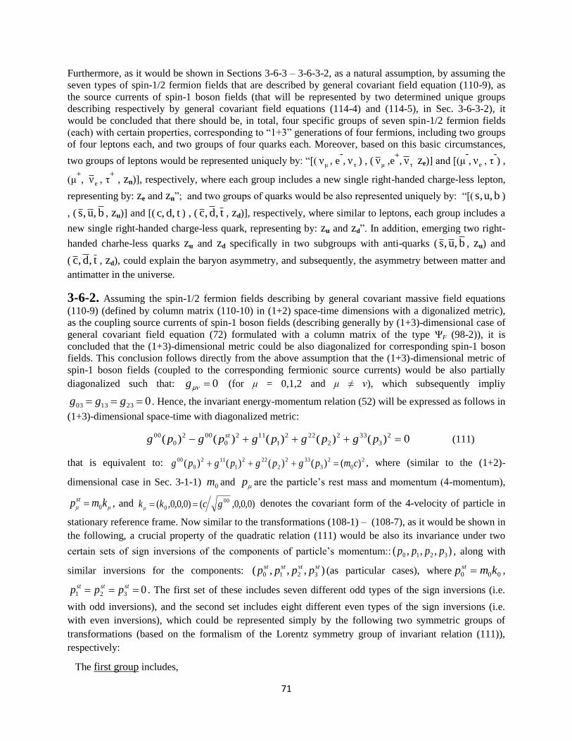
71

Furthermore, as it would be shown in Sections 3-6-3 – 3-6-3-2, as a natural assumption, by assuming the

seven types of spin-1/2 fermion fields that are described by general covariant field equation (110-9), as

the source currents of spin-1 boson fields (that will be represented by two determined unique groups

describing respectively by general covariant field equations (114-4) and (114-5), in Sec. 3-6-3-2), it

would be concluded that there should be, in total, four specific groups of seven spin-1/2 fermion fields

(each) with certain properties, corresponding to ―1+3‖ generations of four fermions, including two groups

of four leptons each, and two groups of four quarks each. Moreover, based on this basic circumstances,

two groups of leptons would be represented uniquely by: ―[( μν , e-, τν ) , ( μν ,e

+, τν ze)] and [(μ

-, eν , τ

-) ,

(μ+, eν , τ

+ , zn)], respectively, where each group includes a new single right-handed charge-less lepton,

representing by: ze and zn‖; and two groups of quarks would be also represented uniquely by: ―[( bu,s, )

, ( b,u,s , zu)] and [( td,c, ) , ( t,d,c , zd)], respectively, where similar to leptons, each group includes a

new single right-handed charge-less quark, representing by: zu and zd‖. In addition, emerging two right-

handed charhe-less quarks zu and zd specifically in two subgroups with anti-quarks ( b,u,s , zu) and

( t,d,c , zd), could explain the baryon asymmetry, and subsequently, the asymmetry between matter and

antimatter in the universe.

3-6-2. Assuming the spin-1/2 fermion fields describing by general covariant massive field equations

(110-9) (defined by column matrix (110-10) in (1+2) space-time dimensions with a digonalized metric),

as the coupling source currents of spin-1 boson fields (describing generally by (1+3)-dimensional case of

general covariant field equation (72) formulated with a column matrix of the type ΨF (98-2)), it is

concluded that the (1+3)-dimensional metric could be also diagonalized for corresponding spin-1 boson

fields. This conclusion follows directly from the above assumption that the (1+3)-dimensional metric of

spin-1 boson fields (coupled to the corresponding fermionic source currents) would be also partially

diagonalized such that: 0μg

(for μ = 0,1,2 and μ ≠ ν), which subsequently impliy

0231303 ggg . Hence, the invariant energy-momentum relation (52) will be expressed as follows in

(1+3)-dimensional space-time with diagonalized metric:

0)()()()()( 2

3

332

2

222

1

112

0

002

0

00 pgpgpgpgpg st (111)

that is equivalent to: 2

0

2

3

332

2

222

1

112

0

00 )()()()()( cmpgpgpgpg , where (similar to the (1+2)-

dimensional case in Sec. 3-1-1) 0m and p are the particle‘s rest mass and momentum (4-momentum),

μ

st

μ kmp 0 , and )0,0,0,()0,0,0,( 00

0 gckk μ denotes the covariant form of the 4-velocity of particle in

stationary reference frame. Now similar to the transformations (108-1) – (108-7), as it would be shown in

the following, a crucial property of the quadratic relation (111) would be also its invariance under two

certain sets of sign inversions of the components of particle‘s momentum:: ),,,( 3210 pppp , along with

similar inversions for the components:

),,,( 3210

stststst pppp (as particular cases), where 000 kmpst ,

0321 ststst ppp . The first set of these includes seven different odd types of the sign inversions (i.e.

with odd inversions), and the second set includes eight different even types of the sign inversions (i.e.

with even inversions), which could be represented simply by the following two symmetric groups of

transformations (based on the formalism of the Lorentz symmetry group of invariant relation (111)),

respectively:

The first group includes,

72

),,,,(),,,,(),,,,( )1(

3

)1(

2

)1(

1

)1(

0

)1(

03210032100 ppppppppppppppp ststst (111-1)

),,,,(),,,,(),,,,( )2(

3

)2(

2

)2(

1

)2(

0

)2(

03210032100 ppppppppppppppp ststst (111-2)

),,,,(),,,,(),,,,( )3(

3

)3(

2

)3(

1

)3(

0

)3(

03210032100 ppppppppppppppp ststst (111-3)

),,,,(),,,,(),,,,( )4(

3

)4(

2

)4(

1

)4(

0

)4(

03210032100 ppppppppppppppp ststst (111-4)

),,,,(),,,,(),,,,( )5(

3

)5(

2

)5(

1

)5(

0

)5(

03210032100 ppppppppppppppp ststst (111-5)

),,,,(),,,,(),,,,( )6(

3

)6(

2

)6(

1

)6(

0

)6(

03210032100 ppppppppppppppp ststst (111-6)

),,,,(),,,,(),,,,( )7(

3

)7(

2

)7(

1

)7(

0

)7(

03210032100 ppppppppppppppp ststst (111-7)

And the second group is given by, respectively:

),,,,(),,,,(),,,,( )8(

3

)8(

2

)8(

1

)8(

0

)8(

03210032100 ppppppppppppppp ststst (111-8)

),,,,(),,,,(),,,,( )9(

3

)9(

2

)9(

1

)9(

0

)9(

03210032100 ppppppppppppppp ststst (111-9)

),,,,(),,,,(),,,,( )10(

3

)10(

2

)10(

1

)10(

0

)10(

03210032100 ppppppppppppppp ststst (111-10)

),,,,(),,,,(),,,,( )11(

3

)11(

2

)11(

1

)11(

0

)11(

03210032100 ppppppppppppppp ststst (111-11)

),,,,(),,,,(),,,,( )12(

3

)12(

2

)12(

1

)12(

0

)12(

03210032100 ppppppppppppppp ststst (111-12)

),,,,(),,,,(),,,,( )13(

3

)13(

2

)13(

1

)13(

0

)13(

03210032100 ppppppppppppppp ststst (111-13)

),,,,(),,,,(),,,,( )14(

3

)14(

2

)14(

1

)14(

0

)14(

03210032100 ppppppppppppppp ststst (111-14)

),,,,(),,,,(),,,,( )15(

3

)15(

2

)15(

1

)15(

0

)15(

03210032100 ppppppppppppppp ststst (111-15)

where, similar to the transformations (108-9) (as equivalent complex representations of the determined

group of transformations (108-1) – (108-7), in (1+2)-dimensional space-time), following noncomplex-

algebraic values of momentum‘s components p ( pp ), the corresponding complex representations of

transformations (111-1) – (111-15) is not a necessary issue in general, however, if the invariant relation

(111) is represented formally by equivalent complex form:

0)()()()()( 33

33

22

22

11

11

00

00

00

00 ppgppgppgppgppg stst (111-16)

then, along with the set fifteen real-valued transformations (111-1) – (111-15), this relation would be also

invariant under these corresponding sets of complex transformations (for 15,...,3,2,1b ):

),,,,(),,,,( )(

3

)(

2

)(

1

)(

0

)(

032100

bbbbstbst ipipipipipppppp ,

),,,,(),,,,( )(

3

)(

2

)(

1

)(

0

)(

032100

bbbbstbst ipipipipipppppp (111-17)

In Sec. 3-6-3, using the transformations (111-1) – (111-15) (along with their corresponding complex

forms (111-17)), a set of fifteen different general covariant field equations would be determined,

including two certain groups of simultaneous field equations (corresponding, respectively, to a group of

seven bispinor fields and a group of eight bispinor fields of spin-1 particles) as the particular cases of the

(1+3)-dimensional form of general covariant field equation (72) (defined with a column matrix of the type

(98-2)).

73

3-6-3. Similar to the set of seven algebraic matrix equations (109) (determined uniquely as the algebraic

equivalent matrix representation of the energy-momentum relation (108)), based on the definite

formulation of the system of linear equation (64) in (1+3) space-time dimensions (formulated in terms of

the matrices (68)), for the energy-momentum relation (111) (along with the transformations (111-1) –

(111-15)) the following two sets of systems of linear equations are also determined uniquely, including

respectively a set of seven and a set of eight systems of equations (with different parametric formalisms).

The general parametric solution of each of these systems of linear equations, obeys also the quadratic

relation (111) (representing a set of fifteen forms, with different parametric formulations, of the general

parametric solutions of quadratic relation (111)). Each of these sets of the systems of linear equations

could be represented uniformly by a matrix equation as follows, respectively:

0)~(

)()(

0

)( 111 bbb

Skmp

, (112-1)

0)~(

)()(

0

)( 222 bbb

Skmp

(112-2)

where 7,...,3,2,11 b , 15,...,9,82 b , kmpbbst )(

0

)( 11 , kmpbbst )(

0

)( 22 , and

~ are two

contravariant 88 real matrices (compatible with matrix representations of the Clifford algebra Cℓ1,3)

defined solely by formulas (65) and (68), and parametric column matrices )( 1b

S and )( 2b

S are also given

uniquely as follows by two distinct expressions (formulated on the basis of definite parametric

formulation of column matrix S (68) in (1+3) space-time dimensions):

s

wvuvu

wvuvu

wvuvu

wvuvu

wvuvu

wvuvu

S

bbbb

bbbb

bbbb

bbbb

bbbb

bbbb

b

)(

)(

)(

0

)(

)(

)(

)(

2

)(

1

)(

1

)(

2

)(

1

)(

3

)(

3

)(

1

)(

3

)(

2

)(

2

)(

3

)(

0

)(

3

)(

3

)(

0

)(

0

)(

2

)(

2

)(

0

)(

0

)(

1

)(

1

)(

0

)(

1111

1111

1111

1111

1111

1111

1 ,

s

wvuvu

wvuvu

wvuvu

wvuvu

wvuvu

wvuvu

S

bbbb

bbbb

bbbb

bbbb

bbbb

bbbb

b

)(

)(

)(

0

)(

)(

)(

)(

2

)(

1

)(

1

)(

2

)(

1

)(

3

)(

3

)(

1

)(

3

)(

2

)(

2

)(

3

)(

0

)(

3

)(

3

)(

0

)(

0

)(

2

)(

2

)(

0

)(

0

)(

1

)(

1

)(

0

)(

2222

2222

2222

2222

2222

2222

2 (113)

which column matrix )( 1b

S includes seven cases with specific parametric formulations expressed

respectively in terms of seven groups of independent arbitrary parameters:)(

2

)(

1

)(

0

)(

2

)(

1

)(

0111111 ,,,,,

bbbbbbvvvuuu ,

and two common arbitrary parameters s and w (i.e. having the same forms in all of the seven cases of

column matrix )( 1b

S ), and column matrix )( 2b

S also includes eight cases with specific parametric

formulations expressed respectively in terms of eight groups of independent arbitrary parameters:)(

2

)(

1

)(

0

)(

2

)(

1

)(

0222222 ,,,,,

bbbbbbvvvuuu , and two common arbitrary parameters s and w (with the same forms in

all of seven cases of the column matrix )( 2b

S ). In addition, similar to the column matrix )(aS represented

soley by formula (109-1), the specific parametric expressions (113) of column matrices )( 1b

S and )( 2b

S in

the formulation of matrix equations (112-1) and (112-2), have been determined specifically by assuming

(as a basic assumption in addition to the systematic natural approach of formulating the matrix equations

(112-1) and (112-2), based on the definite formulation of axiomatically determined matrix equation (64))

the minimum value for total number of arbitrary parameters in both column matrices )( 1b

S and )( 2b

S ,

which implies equivalently the minimum value for total number of arbitrary parameters in all of the

74

fifteen simultaneous (different) cases of matrix equations (112-1) and (112-2) (necessarily with fifteen

independent parametric solutions representing totally a certain set of fifteen different equivalent forms of

the general parametric solution of quadratic relation (111), based on the general conditions of basic

definition of the systems of linear equations corresponding to homogeneous quadratic and higher degree

equations, presented in Sec. 2, and Sections 2-2 – 2-4, 3-1-1 concerning the homogenous quadratic

equations).In the following, similar to the fundamental general covariant field equation (109-2) derived in

Sec. 3-6-1-1, in the derivation of the corresponding field equations (from matrix equations (112-1) and

(112-2), respectively), we will also use the above particular algebraic properties of parameters s and s

which, respectively, have been expressed commonly in the expressions of all of seven simultaneous cases

of matrix equation (112-1), and in the expressions of all of eight cases of matrix equation (112-1).

3-6-3-1. Moreover, similar to the invariant relation (108) and derived matrix equation (109), along with

the transformations (111-1) – (111-15) and algebraic matrix equations (112-1) and (112-2), using the

corresponding complex transformations (111-17), we may also formally have the following equivalent

matrix equations (with the complex expression), respectively (for 7,...,3,2,11 b , 15,...,9,82 b ):

0)~(

)()(

0

)( 111 bbb

Skimpi

, (112-3)

0)~(

)()(

0

)( 222 bbb

Skimpi

(112-4)

where kmp

bbst )(

0

)( 11 , kmp

bbst )(

0

)( 22 . Similar to the matrix equation (109-2), although, based on the

real value of momentum p )( pp , the complex expression of each of the seven cases of algebraic

matrix equation (112-1), and also each of the eight cases of algebraic matrix equation (112-2), definitely,

is not a necessary issue at the present stage. However, since the corresponding momentum operator

p has a complex value (where ),ˆˆ pp in the following, using this basic property of the operator p ,

we derive, distinctly, two certain groups of the general covariant field equations, including a group of

seven different simultaneous field equations from the matrix equations (112-1) and (112-3), and a group

of eight different simultaneous field equations from the matrix equations (112-2) and (112-4) (based on

the general axiomatic approach of derivation of general covariant massive field equations (72) presented

in Sections 3-4 – 3-4-5, and the quantum representations of C, P and T symmetries of this equation,

presented in Sections 3-5 – 3-5-4). Furthermore, in Sec. 3-6-3-2, it would be also shown that each of these

determined two sets of seven and eight simultaneous field equations describe, respectively, a uniform

group of seven spin-1boson fields (corresponding to two left-handed massive charged bosons, along with

their two complementary right-handed bosons; a left-handed massive charge-less boson, along with its

complementary right-handed boson; and a single right-handed massless and charge-less boson), and a

uniform group of eight spin-1 boson field (corresponding to eight massless charged bosons).

Hence, similar to the (1+2)-dimensional general covariant field equation (114) derived in Sec. 3-6-1-1,

based on the axiomatic approach of derivation of the (1+3)-dimensional case of field equation (72)

(defined solely by a column matrix of the form (98-2) in (1+3) space-time dimensions, as shown in Sec.

3-5-2), from the matrix equations (112-1), (112-3) and (112-2), (112-4) (defined solely by column

matrices (113)), also taking into account this basic momentum operator‘s property: pp ˆˆ , the

following two unique groups of seven and eight simultaneous general covariant field equations are

determined solely, respectively:

0)~(

)()(

0

)( 111 b

Z

bbkmDi

(114-1)

0)~()()(

0

)( 222 b

G

bbkmDi

(114-2)

75

specifying by the following two groups of transformations (based on their two corresponding groups of

(sign) transformations (111-1) – (111-7), (111-8) – (111-15) and (111-17)), for 7,...,3,2,11 b and

8,...,3,2,12 b , respectively:

The first group includes,

),,,,(),,,,( 32100

)1(

3

)1(

2

)1(

1

)1(

0

)1(

0 DDDmDDDDmD (114-1-1)

),,,,(),,,,( 32100

)2(

3

)2(

2

)2(

1

)2(

0

)2(

0 DDDmDDDDmD (114-1-2)

),,,,(),,,,( 32100

)3(

3

)3(

2

)3(

1

)3(

0

)3(

0 DDDmDDDDmD (114-1-3)

),,,,(),,,,( 32100

)4(

3

)4(

2

)4(

1

)4(

0

)4(

0

iDiDiDimiDDDDmD (114-1-4)

),,,,(),,,,( 32100

)5(

3

)5(

2

)5(

1

)5(

0

)5(

0

iDiDiDimiDDDDmD (114-1-5)

),,,,(),,,,( 32100

)6(

3

)6(

2

)6(

1

)6(

0

)6(

0

iDiDiDimiDDDDmD (114-1-6)

),,,,(),,,,( 32100

)7(

3

)7(

2

)7(

1

)7(

0

)7(

0

iDiDiDimiDDDDmD (114-1-7)

and the second group is given as follows, respectively:

),,,,(),,,,( 32100

)1(

3

)1(

2

)1(

1

)1(

0

)1(

0 DDDmDDDDmD (114-2-1)

),,,,(),,,,( 32100

)2(

3

)2(

2

)2(

1

)2(

0

)2(

0 DDDmDDDDmD (114-2-2)

),,,,(),,,,( 32100

)3(

3

)3(

2

)3(

1

)3(

0

)3(

0 DDDmDDDDmD (114-2-3)

),,,,(),,,,( 32100

)4(

3

)4(

2

)4(

1

)4(

0

)4(

0 DDDmDDDDmD (114-2-4)

),,,,(),,,,( 32100

)5(

3

)5(

2

)5(

1

)5(

0

)5(

0

iDiDiDimiDDDDmD (114-2-5)

),,,,(),,,,( 32100

)6(

3

)6(

2

)6(

1

)6(

0

)6(

0

iDiDiDimiDDDDmD (114-2-6)

),,,,(),,,,( 32100

)7(

3

)7(

2

)7(

1

)7(

0

)7(

0

iDiDiDimiDDDDmD (114-2-7)

),,,,(),,,,( 32100

)8(

3

)8(

2

)8(

1

)8(

0

)8(

0

iDiDiDimiDDDDmD (114-2-8)

where the column matrices )( 1b

Z and )( 1b

G are also given as follows, written on the basis of definite

formulations of algebraic column matrices (113), in addition to the unique formulation of column matrix

(98-2) (expressing the general representation of column matrices definable in the formulation of (1+3)-

dimensional case of general covariant field equation (72)):

G

bbb

G

b

b

b

b

b

b

b

GZ

bbb

Z

b

b

b

b

b

b

b

Z kmi

DJ

G

G

G

G

G

G

kim

DJ

Z

Z

Z

Z

Z

Z

)(,0

,)(,0 )(

0)()(

)(

31

)(

31

)(

23

)(

30

)(

20

)(

10

)()(

0)()(

)(

31

)(

31

)(

23

)(

30

)(

20

)(

10

)(2

22

2

2

2

2

2

2

2

1

11

1

1

1

1

1

1

1

(114-3)

76

where in all of the seven simultaneous (different) field equations (112-1) formulated with column matrix )( 1b

Z (for 7,...,3,2,11 b ), and also in all of the eight simultaneous (different) field equations (112-2)

formulated with column matrix )( 2b

G (for 8,...,3,2,12 b ), the scalar quantity Z (as initially given

quantity) defines commonly set of seven source currents )( 1b

J , and scalar quantity G also defines

commonly set of eight source currents)( 2b

J .

3-6-3-2. Following the definite formulations of set of seven field equations (114-1), and set of eight

field equations (114-2 ) specified, respectively, by the transformations (114-1-1) – (114-1-7) and (114-2-

1) – (114-2-8), these two sets of the field equations could be represented uniformly by the following

general covariant field equations as well (defined solely in (1+3) space-time dimensions), respectively:

0)~( 0 ZkmDi

(114-4)

0)~( 0 GkmDi

(114-5)

where the column matrices Z and G given by:

,)(,0

0

31

31

23

30

20

10

Z

Z

Z kim

DJ

Z

Z

Z

Z

Z

Z

G

G

G kim

DJ

G

G

G

G

G

G

)(,0

0

31

31

23

30

20

10

(114-6)

and the field strength tensors Z , G and scalars Z

and G

, along with the source currents J and

J are defined as follows:

7

1

)(

1

1

1

b

b

bZZ , ,

8

1

)(

2

2

2

b

b

bGG

,)()(7

1

)(7

1

)(

0)(02

1

1

1

1

1

1

JJkim

Dkim

DIb

b

b

b

Z

bb

Z

.)()(8

1

)(8

1

)(

0)(03

2

2

2

2

2

2

JJkim

Dkim

DIb

b

b

b

G

bb

G

(114-7)

where 2I , 3I are 22 and 33 identity matrices, and2

1

1

b

b

l (for 7,...,3,2,11 b ) are the following

set of seven 22 complex matrices:

77

2

1

1

b

b

l ,

765

4

321

,,

,

,,,

lll

l

lll

1

0

0

1,

0

0,

0

1

1

0

,10

01

,0

0,

0

1

1

0,

0

0

i

i

i

i

i

i

(114-8)

which similar to the set of matrices (110-12) in Sec. 3-6-1-1, represents uniformly a combined gauge

symmetry group of the form: SU(2)LU(2)R , where the subset of three matrices ― 321 ,, ‖ corresponds

to SU(2)L group, and subset of four matrices ― 7654 ,,, ‖ corresponds to U(2)R group.

The matrices 22

)21( bb

(for 8,...,3,2,12 b ) are also the following set of eight 33 complex

matrices equivalent to the Gell-Mann matrices (representing the SU(3) gauge symmetry group):

22 2

1bb

,

876

54

321

,,

,,

,,,

200

010

001

3

1,

00

00

000

,

0

1

0

1

0

0

0

0

0

,

00

000

00

,

0

0

1

0

0

0

1

0

0

,

000

010

001

,

000

00

00

,

0

0

0

0

0

1

0

1

0

i

i

i

i

i

i

(114-9)

Now based on the definite matrix formalisms of the field strength tensors Z and G (114-7)

(described respectively by general covariant massive field equations (114-4) and (114-5)), and on the

basis of C, P and T symmetries of these field equations (as two particular forms of the (1+3)-dimensional

case of tensor field equation (72)), represented by their corresponding quantum operators (defined in

Sections 3-5 – 3-5-4), it would be concluded that the field equation (114-4) describes uniformly a

definite group of seven simultaneous bispinor fields of spin-1 particles (corresponding to seven matrices

7654321 ,,,,,, (114-8)), including, respectively: ―three left-handed massive bosons that could be

denoted by ",~

," ZWW

(represented respectively by three matrices 321 ,, , corresponding with

SU(2)L), a right-handed charge-less spin-1 boson and also three right-handed spin-1 (massive) bosons

denoted by ",~

,," ZWW

(represented respectively by four matrices 7654 ,,, , corresponding with

U(2)R), as the complementary particles of three left-handed bosons represented by the matrices 321 ,, ‖.

In addition, following the definite representations of these determined seven bosons, it could be

concluded that four bosons ),,,( ZWW

correspond to the known bosons including respectively

78

photon (determined as a right-handed charge-less boson, compatible with the positive-frequency

corresponding to the right-handed circular polarization state of photon), and ZWW ,, bosons. Hence,

particles ZWW

,~

,~

represent three new massive spin-1 bosons (where, in particular, Z

is the

complementary right-handed particle of ordinary Z boson), predicted uniquely by this new mathematical

axiomatic approach. Furthermore, the field equation (114-5) also would describe uniformly a definite

group of eight spin-1 boson fields (corresponding respectively to the eight matrices

87654321 ,,,,,,,

, representing SU(3) gauge group).

Furthermore, as noted in Sec. 3-6-1-1, by assuming the group of seven spin-1/2 fermion fields

(described by field equations (110-9) – (110-12)) as the source currents of spin-1 boson fields, it would be

also concluded that the group of seven uniform spin-1 boson fields )( 1b

Z representing by [

),~

,,(),,~

,( ZWWZWW

] (describing by the general covariant field equation (114-4)), and the group

of eight uniform spin-1 boson fields )( 2b

G (describing by general covariant field equations (114-5)), hold

certain properties (including the electrical and color charges, so on) compatible with the known properties

of ordinary bosons ZWW ,, and photon, and also eight gluon fields (with their known definite

properties, including the color charges represented by ‗color octet‘ [35, 36]). In addition, based on the

group representation of three additional new bosons that are predicted uniquely by this new mathematical

axiomatic approach, denoting by: ",~

,~

" ZWW

, these new bosons could have properties similar to the

ordinary bosons ;,, ZWW where in particular new boson Z

(as the complementary right-handed

particle of ordinary Z boson), can mix with Z boson.

Moreover, as mentioned in Sec. 3-6-1-1, by assuming (as a basic natural assumption) the seven types of

spin-1/2 fermion fields describing by general covariant field equation (110-9), as the source currents of

the uniquely determined two groups of seven and eight spin-1 boson fields (describing respectively by

general covariant field equations (114-4) and (114-5)), it would be concluded that there should be, in

total, four specific groups of seven spin-1/2 fermion fields (each) with certain properties, corresponding to

―1+3‖ generations of four fermions, including two groups of four leptons each, and two groups of four

quarks each. Moreover, based on this basic circumstances, two groups of leptons would be represented

uniquely by: ―[( μν , e-, τν ) , ( μν ,e

+, τν ze)] and [(μ

-, eν , τ

-) , (μ

+, eν , τ

+ , zn)], respectively, where each

group includes a new single right-handed charge-less lepton, representing by: ze and zn‖; and two groups

of quarks would be also represented uniquely by: ―[( bu,s, ) , ( b,u,s , zu)] and [( td,c, ) , ( t,d,c , zd)],

respectively, where similar to leptons, each group includes a new single right-handed charge-less quark,

representing by: zu and zd‖. In addition, emerging two right-handed charhe-less quarks zu and zd

specifically in two subgroups with anti-quarks ( b,u,s , zu) and ( t,d,c , zd), could explain the baryon

asymmetry, and subsequently, the asymmetry between matter and antimatter in the universe.

79

4. Conclusion

The main results obtained in this article, are mainly, the outcomes of the new algebraic axiom (17)

(along with the basic assumptions (2) – (3) defined in Sec. 3-1). This new axiom as a definite

generalized form of the ordinary axiom of ―no zero divisors‖ of integral domains (including the

domain of integers), has been formulated soley in terms of square matrices (with integer entries,

appeared as primary objects for representing the integer elements in their corresponding algebraic

axiomatic formalism). In Sec. 3 of this article, as a new mathematical approach to origin of the laws

of nature, using a new basic algebraic axiomatic (matrix) formalism based on the ring theory and

Clifford algebras (presented in Sec.2), “it is shown that certain mathematical forms of fundamental

laws of nature, including laws governing the fundamental forces of nature (represented by a set of

two definite classes of general covariant massive field equations, with new matrix formalisms), are

derived uniquely from only a very few axioms”; where as a basic additional assumption (that is the

assumption (2) in Sec. 3-1), in agreement with the rational Lorentz symmetry group, it has been also

assumed that the components of relativistic energy-momentum (D-momentum) can only take the

rational values. Concerning the basic assumption of rationality of relativistic energy-momentum, it is

necessary to add (as mentioned in Sec. 3-1) that the rational Lorentz symmetry group is not only

dense in the general form of Lorentz group, but also is compatible with the necessary conditions

required basically for the formalism of a consistent relativistic quantum theory [77]. In essence, the

main scheme of the new mathematical axiomatic approach to fundamental laws of nature presented

in Sec. 3, is as follows. First in Sec. 3-1-1, based on the assumption of rationality of D-momentum,

by linearization (along with a parameterization procedure) of the Lorentz invariant energy-

momentum quadratic relation, a unique set of Lorentz invariant systems of homogeneous linear

equations (with matrix formalisms compatible with certain Clifford, and symmetric algebras) has

been derived. Then in Sec. 3-4, by first quantization (followed by a basic procedure of minimal

coupling to space-time geometry) of these determined systems of linear equations, a set of two

classes of general covariant massive (tensor) field equations (with matrix formalisms compatible

with certain Clifford, and Weyl algebras) has been derived uniquely as well. Each class of the

derived general covariant field equations also includes a definite form of torsion field appeared as

generator of the corresponding field‘ invariant mass. In addition, in Sections 3-4 – 3-5, it has been

shown that the (1+3)-dimensional cases of two classes of derived field equations represent a new

general covariant massive formalism of bispinor fields of spin-2, and spin-1 particles, respectively. In

fact, these uniquely determined bispinor fields represent a unique set of new generalized massive forms of

the laws governing the fundamental forces of nature, including the Einstein (gravitational), Maxwell

(electromagnetic) and Yang-Mills (nuclear) field equations. Moreover, it has been also shown that the

(1+2)-dimensional cases of two classes of these field equations represent (asymptotically) a new general

covariant massive formalism of bispinor fields of spin-3/2 and spin-1/2 particles, respectively,

corresponding to the Dirac and Rarita–Schwinger equations. As a particular consequence, in Sec. 3-4-2, it has been shown that a certain massive formalism of general

relativity – with a definite form of torsion field appeared originally as the generator of gravitational

field‘s invariant mass – is obtained only by first quantization (followed by a basic procedure of minimal

coupling to space-time geometry) of a certain set of special relativistic algebraic matrix equations. In Sec.

3-4-4, it has been also proved that Lagrangian densities specified for the originally derived new massive

forms of the Maxwell, Yang-Mills and Dirac field equations, are also gauge invariant, where the invariant

mass of each field is generated solely by the corresponding torsion field. In addition, in Sec. 3-4-5, in

80

agreement with recent astronomical data, a new particular form of massive boson has been identified

(corresponding to U(1) gauge group) with invariant mass: mγ ≈ 4.90571×10-50kg, which is specially

generated by a coupled torsion field of the background space-time geometry.

Moreover, in Sec. 3-5-2, based on the definite mathematical formalism of this new axiomatic

approach, along with the C, P and T symmetries (represented basically by the corresponding

quantum matrix operators) of uniquely derived two fundamental classes of general covariant field

equations, it has been concluded that the universe could be realized solely with the (1+2) and (1+3)-

dimensional space-times (where this conclusion, in particular, is based on the time-reversal

symmetry). In Sections 3-5-3 and 3-5-4, it has been proved that 'CPT' is the only (unique)

combination of C, P, and T symmetries that could be defined as a symmetry for interacting fields.. In

addition, in Sec. 3-5-4, on the basis of these discrete symmetries of derived field equations, it has

been also shown that only left-handed particle fields (along with their complementary right-handed

fields) could be coupled to the corresponding (any) source currents. Furthermore, in Sec. 3-6, it has

been shown that metric of the background space-time is diagonalized for the uniquely derived

fermion field equations (defined and expressed solely in (1+2)-dimensional space-time), where this

property generates a certain set of additional symmetries corresponding uniquely to the

SU(2)LU(2)R symmetry group for spin-1/2 fermion fields (representing ―1+3‖ generations of four

fermions, including a group of eight leptons and a group of eight quarks), and also the SU(2)LU(2)R

and SU(3) gauge symmetry groups for spin-1 boson fields coupled to the spin-1/2 fermionic source

currents. Hence, along with the known elementary particles, eight new elementary particles,

including: four new charge-less right-handed spin-1/2 fermions (two leptons and two quarks,

represented by ―ze , zn and zu , zd‖), a spin-3/2 fermion, and also three new spin-1 massive bosons

(represented by ",~

,~

" ZWW

, where in particular, the new boson Z

is complementary right-

handed particle of ordinary Z boson), have been predicted uniquely by this fundamental axiomatic

approach. As a particular result, in Sec. 3-4-2, based on the definite and unique formulation of the

derived Maxwell‘s equations (and also determined Yang-Mills equations, represented uniquely with

two specific forms of gauge symmetries, in 3-6-3-2), it has been also concluded generally that

magnetic monopoles could not exist in nature.

The new results obtained in this article, which are connecting with a number of longstanding

essential issues in science and philosophy, demonstrate the wide efficiency of a new fundamental

algebraic-axiomatic formalism presented in Sec. 2 of this article.

Acknowledgment Special thanks are extended to Prof. and Academician Vitaly L. Ginzburg (Russia), Prof. and

Academician Dmitry V. Shirkov (Russia), Prof. Leonid A . Shelepin (Russia), Prof. Vladimir Ya.

Fainberg (Russia), Prof. Wolfgang Rindler (USA), Prof. Roman W. Jackiw (USA), Prof. Roger

Penrose (UK), Prof. Steven Weinberg (USA), Prof. Ezra T. Newman (USA), Prof. Graham Jameson

(UK), Prof. Sergey A. Reshetnjak (Russia), Prof. Sir Michael Atiyah (UK) (who, in particular, kindly

encouraged me to continue this work as a new unorthodox mathematical approach to fundamental

physics), and many others for their support and valuable guidance during my studies and research.

***********************

81

This article has been invited and presented at the following international conferences:

The 2016 SIAM International Conference on Mathematical Aspects of Materials Science, Philadelphia,

USA, 2016. (https://www.siam.org/meetings/ms16)

The 17th International Conference on Quantum Foundations: Quantum and Beyond, International Centre

for Mathematical Modeling in Physics, Engineering and Cognitive Sciences (ICMM), Linnaeus

University, Sweden, 2016. (https://lnu.se/en/qb/)

The 4th International Conference on New Frontiers in Physics, CERN Organized and Supported

Conference (Europe), ICNFP-2015. (https://indico.cern.ch/e/icnfp2015/)

The 2016 International Conference on Algebraic Geometry and Mathematical Physics, University of

Tromsø, Norway, 2016. (https://site.uit.no/)

The XXXVII Max Born International Symposium, International Conference on Non-commutative

Geometry, Quantum Symmetries and Quantum Gravity (II), Wroclaw University, Poland, 2016.

(http://ift.uni.wroc.pl/~mborn37/)

The 2016 GRavitational-wave Astronomy International Conference in Paris, Institute d‘Astrophysique

de Paris (IAP), The University of Paris VI - Sorbonne University, CNRS, LERU, EUA, Paris, France,

‗Supported by the European Union's 7th

Framework Program: FP7/PEOPLE-2011-CIG,‘ 2016.

(http://www.iap.fr/vie_scientifique/ateliers/GravitationalWave/2016/scripts/abstract.aspx)

The 22nd

Internnational Australian Institute of Physics Congress (AIP), University of Queensland,

Brisbane, Australia, 2016. (http://appc-aip2016.org.au)

The 21st International Conference on General Relativity and Gravitation, Columbia University, New

York, USA, 2016. (http://www.gr21.org)

References:

[1]- Zahedi, Ramin A., ―Linearization Method in the Ring Theory‖, Russian Academy of Sciences

(RAS), Bulletin of the Lebedev Physics Institute, New York, Springer-Verlag, No. 5-6, 1997.

[2]- Zahedi, Ramin A., ―On Applied Aspects of the Ring Theory‖, Russian Academy of Sciences (RAS),

Bulletin of the Lebedev Physics Institute, New York, Springer-Verlag, No. 3-4, 1997.

[3]- Zahedi, Ramin A., ―On the Connection Between Methods of the Ring Theory and the Group

Approach‖, Russian Academy of Sciences (RAS), Bulletin of the Lebedev Physics Institute, New York,

Springer-Verlag, No. 7-8, 1997.

[4]- Zahedi, Ramin A., ―The Linearization Method Based on the Ring Theory and its Applications in

Physics‖, Russian Academy of Sciences (RAS) Publs., Russia, 1998;

http://dlib.rsl.ru/viewer/01000049410 .

[5]- Durbin, J. R., ―Modern Algebra: An Introduction‖, (3rd ed.), John Wiley and Sons, USA, 1993;

Blyth , T.S.; Robertson, E.F. ―Groups, rings and fields: Algebra through practice,‖ Book 3. Cambridge

University Press, UK, 1985.

[6]- Dickson, L. E., ―History of the Theory of Numbers‖, Volume II: Diophantine Analysis, Mineola,

Dover Publications, NY, USA, 2005.

[7]- Mordell, L. J., ―Diophantine Equations‖, Pure and Applied Mathematics, 30, Academic Press, 1969.

[8]- Ireland, K.; Rosen, M. ―A Classical Introduction to Modern Number Theory‖, 2nd ed., Springer-

Verlag, New York, USA, 1998.

[9]- Guidry, M. W. ―Gauge Field Theories: An Introduction with Applications‖, John Wiley&Sons, 1991.

[10]- Byrnes, J. (ed.) ―Computational Noncommutative Algebra and Applications‖, Springer-Verlag,

pp. 363-387, 2004.

[11]- Bourbaki, N., ―Algebra‖, Berlin, New York, Springer-Verlag, 1988.

[12]- McMahon, D., ―Quantum Field Theory‖, Mc Graw Hill (USA), 2008.

[13]- Woan, G., "The Cambridge Handbook of Physics Formulas", Cambridge University Press, 2010.

[14]- Martin, B. R.; Shaw, G., ―Particle Physics‖, Manchester Physics Series (3rd ed.), John Wiley &

Sons, USA, 2008.

82

[15]- Noyes, H. P.; van den Berg, J. C., ―Bit-string Physics: A Finite and Discrete Approach to Natural

Philosophy‖, World Scientific, 2001.

[16]- Morel, John Henry, ―The Manual of Quants: Discrete Physics and Quantitative Analysis‖, Laguna

Beach, CA (USA), 2009.

[17]- Noyes, H. P., ―Some thoughts on discrete physics and the reconstruction of quantum mechanics‖,

Stanford Linear Accelerator Center (Menlo Park), CA (USA), SLAC-PUB--7145 (C96-06-03.10), 1996.

[18]- Kauffman, L. H., "Knots and Physics", 3rd Edition, World Scientific, 2001.

[19]- Svozil, K., ―Randomness & Undecidability in Physics: Chapter 3: Discrete Physics‖, World

Scientific, 1993.

[20]- Ilachinski, A., ―Cellular Automata: A Discrete Universe‖, World Scientific, 2001.

[21]- Amoroso, R. L.; Kauffman, L. H.; Rowlands, P., ―The Physics of Reality: Space, Time, Matter;

Section I: Laws of Forms, Majorana Fermions, and Discrete Physics‖, Cosmos, World Scientific, 2013.

[22]- Zenil, H.; Penrose, R., ―A Computable Universe: Understanding and Exploring Nature as

Computation‖, World Scientific, 2013.

[23]- Penrose, R.; Rindler , W., ―Spinors and Space-Time‖, vol. 1, 2, Cambridge Uni. Press, 1984, 1986.

[24]- Fulling, S.A., ―Aspects of Quantum Field Theory in Curved Space–Time‖, Cambridge University

Press, 1996.

[25]- Freedman, D. Z.; van Proeyen, A., ‗Supergravity‖, Cambridge University Press, 2012.

[26]- Lawson, H. B., Jr.; Michelsohn, Marie-L., ―Spin Geometry,‖ Princeton University Press, 1989.

[27]- Straumann, N., ―General Relativity: With Applications to Astrophysics‖, Springer-Verlag, 2013.

[28]- Wald, R. M., ―General Relativity‖, University of Chicago Press, 2010.

[29]- Elton, D.; Vassiliev, D., ―The Dirac equation without spinors‖, Operator Theory: Advances and

Applications, Springer-Verlag, vol. 110. pp. 133-152, 1999.

[30]- Griesshammer, H.W.; Lehmann, D.; Seeger, M., ―Introduction to Supersymmetry and Exact

Nonperturbative Results in SUSY-QCD‖, Lecture Notes in Physics, 481, Springer-Verlag, 1997.

[31]- Illge, R., ―Massive Fields of Arbitrary Spin in Curved Space-Times‖, Commun. Math. Phys., 158,

Springer-Verlag, 1993.

[32]- Pilkuhn, H., "Relativistic Quantum Mechanics", Springer-Verlag, p.156 , 2003.

[33]- Weinberg, S., Phys. Rev. 133, B1318, 1964; 134, B882, 1964.

[34]- Joos, H., "Zur Darstellungstheorie der inhomogenen Lorentzgruppe als Grundlage

quantenmechanischer Kinematik", Fortschr. Phys. 10, pp.65-146, 1962.

[35]- Weinberg, S., "The Quantum Theory of Fields", Cambridge University Press, 1995.

[36]- Pal, P. B., "An Introductory Course of Particle Physics", CRC Press, Taylor & Francis Publications ,

p. 151, 2014.

[37]- Ticciati, R., "Quantum Field Theory for Mathematicians", Cambridge University Press, 1999.

[38]- Devreese, J.T.; Peeters, F.M., ―The Physics of the Two-Dimensional Electron Gas‖, Springer-

Verlag, 2012.

[39]- Andrei, E.Y., ―Two-Dimensional Electron Systems: on Helium and other Cryogenic Substrates‖,

Springer-Verlag, 2012.

[40]- Tesser, S. B., ―Generalized Clifford algebras and their representations‖, Micali, A.; Boudet, R.;

Helmstetter, J. (eds.), Clifford algebras and their applications in mathematical physics, Springer-Verlog,

pp. 133–141, 2011.

[41]- Ramakrishnan, A., ―Generalized Clifford Algebra and its applications – A new approach to internal

quantum numbers‖, Proceedings of the Conference on Clifford algebra, its Generalization and

Applications, (January 30 – February 1, 1971), Matscience (IMSc), Madras, 20, pp. 87–96, 1971.

[42]- Morris, O., ―On a Generalized Clifford Algebra I & II‖, Quart. J. Math (Oxford), 18, pp. 7–12,

1967, 19, pp. 289–299, 1968.

[43]- Pappacena, C. J., ―Matrix pencils and a generalized Clifford algebra‖, Linear Algebra and its

Applications 313 (1-3), Elsevier, pp. 1–20, 2000.

[44]- Chapman, A.; Kuo, J., ―On the generalized Clifford algebra of a monic polynomial‖, Linear Algebra

and its Applications 471, Elsevier, pp. 184–202, 2015.

83

[45]- Coskun, E.; Kulkarni, R. S.; Mustopa, Y., ―On representations of Clifford algebras of Ternary cubic

forms‖, Contemporary Mathematics, Vol. 562, Amer. Math. Soc., pp. 91–99, 2012.

[46]- Ablamowicz, R.; Parra, J.; Lounesto, P., (eds.) ―Clifford Algebras with Numeric and Symbolic

Computations‖, Springer-Verlog, 2012.

[47]- Smith, T., ―Decomposition of generalized Clifford algebras‖, Quart. J. Math., Oxford 42, pp.105-

112, 1991.

[48]- Witten, E., ―Three Lectures On Topological Phases Of Matter‖, arXiv:1510.07698, 2015.

[49]- Sidharth, B.; Altaisky, M.V., ―Frontiers of Fundamental Physics 4‖, Springer-Verlog, 2001.

[50]- Wigner, E., ―The Unreasonable Effectiveness of Mathematics in the Natural Sciences‖,

Communications in Pure and Applied Mathematics, vol. 13, no. 1, John Wiley & Sons, New York, 1960.

[51]- Lucas, J. R., ―Gödel's Incompleteness Theorems‖, Oxford University Press, 1999.

[52]- Kaye, R., ―Models of Peano arithmetic‖, Oxford University Press, 1991.

[53]- Mendelson, E., ―Introduction to Mathematical Logic‖, 4th ed., Chapman & Hall, 1997.

[54]- Smullyan, R., ―Conceptual Roots of Mathematics‖, Routledge, 1991.

[55]- Oxford English Dictionary, "Law of Nature", Oxford University Press, 2015.

[56]- Swartz, N,. "The Concept of Physical Law", Cambridge Uni. Press, New York, 1985.

[57]- Barrow, J., "Theories of Everything: The Quest for Ultimate Explanations", 2nd Ed. (New Ed.),

Oxford University Press, 2007.

[58]- Frampton, P., ―Gauge Field Theories‖, 3rd

ed., Wiley-VCH, 2008.

[59]- Forshaw, J. R.; Smith, A.G., ―Dynamics and Relativity‖, Manchester Physics Series, John Wiley &

Sons, 2009.

[60]- Fresneda, R.; Baldiotti, M. C.; Pereira, T. S., "Maxwell Field with Torsion", Brazilian Journal of

Physics, vol. 45, No. 3, Springer-Verlog, pp. 353-358, 2015.

[61]- Gasperini, M.,Gen. Relat. Gravit. 16(11), 1031, 1984; (also see : A.M. Nobili, D.M. Lucchesi, M.T.

Crosta, M. Shao, S.G. Turyshev, R. Peron, G. Catastini, A. Anselmi, G. Zavattini, Am. J. Phys. 81(7),

527, 2013).

[62]- Hehl, F.W.; Obukhov, Y.N., "How Does the Electromagnetic Field Couple to Gravity, in Particular

to Metric, Nonmetricity, Torsion, and Curvature? in Gyros, Clocks, Interferometers...: Testing Relativistic

Gravity in Space", Lecture Notes in Physics, Volume 562, Springer-Verlog, Berlin, pp. 479–504, 2001.

[63]- Baldiotti, M. C.; Elias, W. S.; Molina, C.; Pereira, T. S., Phys. Rev. D 90(10), 104025, 2014.

[64]- Deser, S.; Jackiw, R.; Templeton, S., "Three-Dimensional Massive Gauge Theories", Phys. Rev.

Lett., No. 48, pp. 975-978, 1982; Deser, S.; Jackiw, R.; t‘Hooft, G., ―Three-Dimensional Einstein

Gravity: Dynamics of Flat Space‖, Annals of Physics, No. 152, pp. 220-235, 1984.

[65]- Jackiw, R.; Pi, S.-Y., "Chern–Simons modification of general relativity", Phys.Rev., D68, 2003.

[67]- Hollands, S., "Renormalized Quantum Yang-Mills Fields in Curved Spacetime", Rev. Math. Phys.,

20, pp. 1033-1172, 2008.

[68]- Bialinicki, B., "On the Wave Function of the Photon", ACTA PIIYSICA POLONICA A, Vol. 86 ,

No. 1-2, pp. 97-116, 1994; (see also: Raymer, M. G.; Smith, B. J., "The Maxwell wave function of the

photon", Proc. SPIE 5866, pp. 293-297, 2005; Gersten A., ―Maxwell Equations—The One-Photon

Quantum Equation‖, Foundations of Physics, 31 (8), pp. 1211-1231, 2001).

[69]- Mohr, P. J., "Solutions of the Maxwell equations and photon wave functions", Annals of Physics

325, pp. 607-663, 2010.

[70]- Jaffe, A.; Witten, E., "Quantum Yang–Mills theory", In: Carlson, J.; Jaffe, A.; Wiles, A. (Eds.),

The Millennium Prize Problems, American Mathematical Society, Providence, RI, pp. 129-152, 2006.

[71]- Sushkov, A. O.; Kim, W. J.; Dalvit, D. A. R.; Lamoreaux, S. K., "New Experimental Limits on

Non-Newtonian Forces in the Micrometer Range", Physical Review Letters, 107 (17): 171101, 2011.

[72]- Hehl, F. W., "Four lectures in Poincare gauge field theory", In Cosmology and Gravitation,

Bergmann, P. G.; de Sabbata, V. (Eds.), Plenum Press, New York, pp. 5-61, 1980.

[73]- Aldrovandi, R.; Pereira, J. G., "An Introduction to Geometrical Physics", World Scientific,

Singapore, 1995.

84

[74]- de Andrade, V. C.; Pereira, J. G., "Gravitational Lorentz Force and the Description of the

Gravitational Interaction", Phys. Rev. D 56, pp. 4689-4695,1997.

[75]- Kouwn, S.; Oh, P.; Park, Chan-G., "Massive Photon and Dark Energy", Phys. Rev. D 93, 083012, 2016;

(See also: Chandler, David L., "Seeing the dark: New MIT-led experiment could finally shed light on the

mysteries of dark matter", MIT News, 2013; https://news.mit.edu/2013/dark-matter-1025 ,

https://dmtpc.mit.edu/DarkLight/DarkLightProposal_PAC39.pdf).

[76]- Zahedi, R., ―On the Logical Origin of the Laws Governing the Fundamental Forces of Nature: A New

Axiomatic Matrix Approach‖, Preprint, Hokkaido University Publs., 2015;1

(http://Eprints.lib.Hokudai.ac.jp/dspace/handle/ 2115/59279/, https://inspirehep.net/record/1387680/ ). [77]- Hill, E. L., ―Relativistic Theory of Discrete Momentum Space and Discrete Space-Time‖, Phys. Rev., Vol. 100, No. 6, pp. 1780-1783, 1955. [78]- Rindler , W., ―Relativity: SPECIAL, GENERAL, AND COSMOLOGICAL‖, Oxford University

Press, New York, 2006.

------------------------------------------------------------------------------------------------------------------------------------------------------------------------------

1. External URLs (Including preprints and earlier published versions of this article):

https://cds.CERN.ch/record/1980381/, https://hal-Univ-Paris3.archives-ouvertes.fr/USPC/hal-01547739,

https://INSPIREHEP.net/record/1387680, http://philsci-archive.PITT.edu/11497, www.IJQF.org/archives/3495,

https://LNU.se/contentassets/1489145f113348f382202fbf0d1d4094/qb-abstracts-compiled-160613.pdf ,

https://citeseerx.ist.PSU.edu/viewdoc/summary?doi=10.1.1.675.2202, http://philpapers.cdp.UWO.ca/rec/zahotl,

http://www.NoeticadvAncedStudies.US/ZahediX.pdf, https://Dumas.CCSD.CNRS.fr/TDS-MACS/hal-01547739,

https://dx.doi.org/10.17605/OSF.IO/PQGA9, https://hal-Univ-Paris3.archives-ouvertes.fr/USPC/hal-01547739,

http://mts-srep.nature.com/srep_files/2017/07/20/00174434/00/174434_0_related_ms_4909193_pttcpw.pdf ,

https://indico.CERN.ch/event/344173/contribution/1740565/attachments/1140145/1726912/R.A.Zahedi--

Forces.of.Nature.Laws-Jan.2015-signed.pdf (updated version).

85

Appendix A.

The matrix equation (64) in Minkowski flat space-time (with metric signature (+ – –...–)) would be

represented simply by:

0)( 0 SImp (A)

where I is the identity matrix, and column matrix S is defined uniquely by formulas (66) – (70),… in

(1+1), (1+2), (1+3), (1+4), (1+5),… space-time dimensions. The general contravariant forms of real

matrices that generate the Clifford algebra Cℓ1,N (for N ≥ 2) in (1+N)-dimensional space-time, are

(as mentioned in Sec. 3-3), are expressed by formulas (66) – (70),… in various space-times dimensions.

Moreover, following the axiomatic approach of derivation of matrix equation (64), matrices in

Minkowski flat space-time also hold the Hermiticity and anti-Hermiticity properties such that: )( 00 (compatible with 1)( 20 ), and

)( (compatible with 1)( 2 , for μ

=1,2,3,…).

These matrices in the (1+1), (1+2), (1+3) and (1+4)-dimensional Minkowski space-time (as special cases

of their general contravariant forms (65) – (69),…), have the following representations, respectively:

- For (1+1)-dimensional space-time we have:

01

10,

10

0110 (A-1)

- For (1+2)-dimensional case we get:

.

0010

0001

1000

0100

0

0

,

0001

0010

0100

1000

0

0

,

1000

0100

0010

0001

)(0

0

01

01

2

32

32

1

10

10

0

(A-2)

86

- In (1+3) dimensions, we have:

,

10000000

01000000

00100000

00010000

00001000

00000100

00000010

00000001

)(0

010

10

0

,

00000001

00000010

00000100

00001000

00010000

00100000

01000000

10000000

0

032

32

1

,

00000010

00000001

00001000

00000100

00100000

00010000

10000000

01000000

0

054

54

2

.

00000100

00001000

00000001

00000010

01000000

10000000

00010000

00100000

0

076

76

3

(A-3)

87

- In (1+4) dimensions, these matrices given by:

,

1000000000000000

0100000000000000

0010000000000000

0001000000000000

0000100000000000

0000010000000000

0000001000000000

0000000100000000

0000000010000000

0000000001000000

0000000000100000

0000000000010000

0000000000001000

0000000000000100

0000000000000010

0000000000000001

0

,

0000000000000001

0000000000000010

0000000000000100

0000000000001000

0000000000010000

0000000000100000

0000000001000000

0000000010000000

0000000100000000

0000001000000000

0000010000000000

0000100000000000

0001000000000000

0010000000000000

0100000000000000

1000000000000000

1

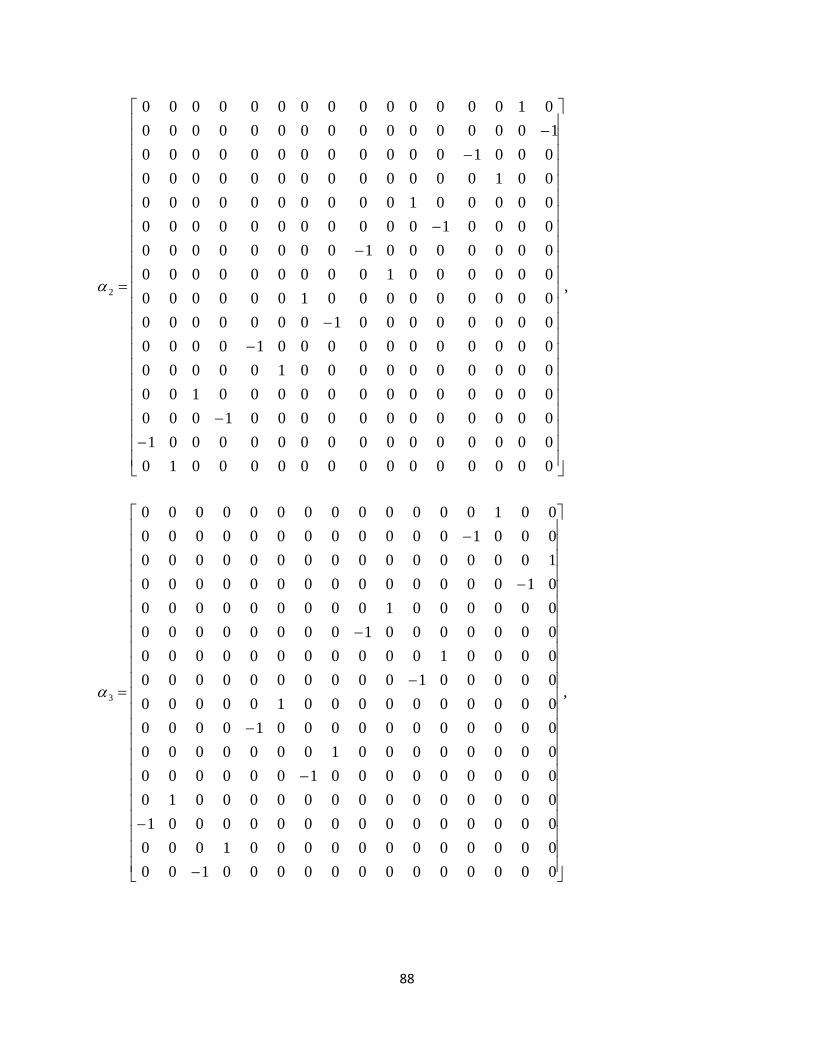
88

,

0000000000000010

0000000000000001

0000000000001000

0000000000000100

0000000000100000

0000000000010000

0000000010000000

0000000001000000

0000001000000000

0000000100000000

0000100000000000

0000010000000000

0010000000000000

0001000000000000

1000000000000000

0100000000000000

2

,

0000000000000100

0000000000001000

0000000000000001

0000000000000010

0000000001000000

0000000010000000

0000000000010000

0000000000100000

0000010000000000

0000100000000000

0000000100000000

0000001000000000

0100000000000000

1000000000000000

0001000000000000

0010000000000000

3

89

,

0000000000010000

0000000000100000

0000000001000000

0000000010000000

0000000000000001

0000000000000010

0000000000000100

0000000000001000

0001000000000000

0010000000000000

0100000000000000

1000000000000000

0000000100000000

0000001000000000

0000010000000000

0000100000000000

4

(A-4).