Carnegie Mellon UniversityResearch Showcase @ CMU

Tepper School of Business

5-1992

Inflation and Money in BrazilAllan H. MeltzerCarnegie Mellon University, am05@andrew.cmu.edu

Follow this and additional works at: http://repository.cmu.edu/tepper

Part of the Economic Policy Commons, and the Industrial Organization Commons

This Conference Proceeding is brought to you for free and open access by Research Showcase @ CMU. It has been accepted for inclusion in TepperSchool of Business by an authorized administrator of Research Showcase @ CMU. For more information, please contact research-showcase@andrew.cmu.edu.

Published InN. Liviatan, (ed.), Proceedings of a Conference on Currency Substitution and Currency Boards, the World Bank, 1993, as "Inflationand Stabilization in Brazil".

Revised August 1991 and May 1992

INFLATION AND MONEY IN BRAZIL

by Allan H. Meltzer*

Executive Summary

(1) Brazil's anti-inflation policy has frequently confused symptoms with causes and relied on one-time stop gaps. At times, these measures were based on the belief that inflation is an inertial process that can be stopped (or slowed) permanently by breaking the momentum. Policies based on this belief such as freezing wages and prices, changing the currency unit or freezing part of the stock of financial assets have failed to stop inflation. However, the last of these measures-the Collor plan-prevented inflation from becoming hyperinflation in 1990.

(2) Brazil's inflation in the 1980s was almost entirely monetary. On average, prices and money rose at the same rate and per capita output changed very little. The average change in velocity is small relative to changes in money, prices and nominal output.

(3) For broad measures of money, the trend of velocity is negative in the 1980s. Hence, on average, movements of these measures of velocity lowered the rate of inflation. Moreover, annual changes in velocity are small, and the variability of velocity is a small fraction of the variability of inflation and money growth.

(4) Brazil has avoided the rapid increase in velocity and the flight from money characterically found in countries with sustained high inflation. Indexation of most asset returns and asset values is the most likely explanation of this difference.

(5) The main source of inflation is the financing of total government spending and subsidies. The financing mechanism differed during the decade, but the result was a sustained rapid increase in government debt held by the public (including financial institutions) and in government debt held by the central bank. The latter was

'Valeriano Garcia made helpful comments on an earlier draft.

the main source of growth of base money and money. (6) The central bank had little choice about expanding money during this period

given the rules and procedures under which monetary policy was conducted. These rules and procedures changed several times but none of the changes established the requisites for price stability or low inflation.

(7) Brazil began to transfer a sizeable share of GDP abroad before Mexico's default in 1982. The large transfers reflected the rise in real interest rates in the world economy and the policy of borrowing substantial amounts abroad in the early 1980s.

(8) Past Brazilian programs or plans to control inflation did not reduce the government financing requirement permanently. Measures of the government financing requirement in the first quarter 1991 show this measure of the deficit equal to at least 8% of GDP. This estimate does not include several, large deferred items including the financial assets frozen in March 1990. This measure of the government's fiscal position differs markedly from the position shown in the government's fiscal accounts. Data for interest rates and rates of inflation in 1991 suggest that the markets anticipate inflation to continue at rates consistent with the government financing requirement not the reported budget data.

(9) Reduction in spending have been made by the Collor government. Some of these reductions are more in the nature of postponements than permanent reductions in spending. The deferred spending includes capital projects to serve a growing population. I estimate that after the current recession, if spending remains constant in dollars, the budget would have a monthly surplus of US $1.2 billion before payment of deferred interest and the unblocking of frozen accounts. This surplus if sustained would not be sufficient to service debt and other obligations omitted from the budget unless domestic inflation and interest rates can be brought close to world levels.

(10) Variability of velocity was not large enough to render control of inflation difficult if Brazil had instituted control of government spending, the government financing requirement and money growth.

(11) The procedures under which government securities are sold and the rules for repurchase were changed in 1991. Prior to the change, holders could resell Treasury obligations to the central bank at their option when inflation rose. This option

2

has been eliminated, but the government must be willing to let interest rates rise or money growth will remain excessive.

(12) The government should close the monetary operations of the central bank and institute a currency board. The board would issue cruzeiros only in exchange for convertible foreign money at prevailing exchange rates. The nominal exchange rate for the cruzeiro would be pegged to the U.S. dollar. All new issues of money would be backed 100% by foreign currency. Principal results would be: inflation and market interest rates would be reduced to near the U.S. level; interest payments would fall substantially, lowering the government financing requirement; the government deficit would be financed only from domestic saving and foreign capital, so spending would be controlled; Brazil would retain the seigniorage on its currency but lose the inflation tax; the program would be a strong commitment to a credible anti-inflation policy.

Postscript added May 1992: At the World Bank Conference; some participants questioned the use of end

of year measures of money in the computation of velocity measures. They urged the use of average money stock to compare to average annual output. For M2, M3, and M4, the revised measures are higher, of course, but the yearly pattern is the same and, most importantly, the trend of velocity remains negative until 1989, as before. The revised data for Mi, M2 and M4 are in an appendix at the end of the paper.

Mi velocity is more variable and has a more pronounced positive trend when

average money stock is used. The trend of velocity shows a pattern similar to the

pattern in countries with high inflation. These data reinforce the conclusion about

indexation as a factor affecting the relative movements of Mi and other velocity

measures. Comments about the variability of Mi velocity are affected. The variance of

Mi velocity increased.

3

Introduction

Brazil's inflation rate has increased rapidly since the middle of the 1970s. From an average rate of about 15% per year, inflation jumped to about 45% per year from 1974 to 1979, to more than 100% from 1979 to 1983, then to an average annual rate of 200% from 1983 through 1987, and finally to the hyperinflation rates of 1989 and 1990. For the eleven years 1980-1990, the average rate of inflation (INPC) was 529%, and for the last five complete years, 980%.

Growth of real per capita income for the years 1980-90 (inclusive) and for 1986-90 is approximately zero. The average growth of money is similar to the rate of inflation for the eleven years with some variation depending on the concept of money used. Using the narrowest definition of money, the monetary base (as conventionally defined), average annual money growth is 541% for 1980-90 inclusive. Government debt held by the public increased somewhat faster, at an average rate of 670% per year during this period.

Table 1 shows a different set of measures than the averages just discussed -compound average annual rates of growth for debt, inflation, and several definitions of money for five and nine year periods ending in 1990.1 There are differences in the average rates of money growth particularly in the more recent period, but for the period as a whole all are similar to the compound average annual rate of inflation and the growth of nominal GDP.

From these data and the relatively small change in real income or per capita real income, we can reach five conclusions. First, monetary velocity changed very little during the period of high inflation. The inflation is dominantly monetary. Second, velocity changed very little in most years, so it explains very little of the annual rates of inflation. For broad definitions of money, the trend in velocity is negative. (See Chart 4 below). Third, as suggested by the data on velocity and per capita income, real money

iData are from Brazil: Selected Issues of the Financial Sector. World Bank; March 26,1990, Table 2, App. 5 and Brazil Economic Program v. 28, March 1991, Central Bank of Brazil.

4

Table 1 Percentage Rates of Change of Money, Debt and Prices«

Base Mi

1981-90 159 154

Ma 154

M4 Debt*» Prices GDP

154 153 161 158

1985-90 210 200 191 189 180 206 203

«Compound average annual rates of change, end of year data bPrivately held government debt

balances changed very little on average; there is no evidence of the substantial flight from money that typically characterizes high or hyper-inflations. This is true for either the recent five years or the nine year period taken as a whole. Fourth, the different definitions of money rose at relatively similar rates. Hence, the ratio of money to the monetary base (the money multiplier) changed very little on average, and for a narrow definition of money, there is little monthly variation (Chart 2). This, too, suggests that the inflation process was dominantly a monetary process that was not much affected, on average, by changes in intermediation or the many changes in laws and regulations affecting the economy or the banking and financial system. Fifth, the impulse for inflation came from the financing of the government including the operations of the Bank of Brazil until the mid-1980s and the operations of state banks. The mechanisms of finance differed over the period, but the result was a rapid increase in the government debt held by the public (including financial institutions) and in government debt held by the central bank. The latter was the main source of the growth of the monetary base; the central bank purchased government debt from the market by issuing base money. Through most of the period, the central bank had little choice about making these purchases, given the rules and procedures under which policy was conducted. These rules and procedures were not immutable. They

5

changed several times. None of the changes established the requisites for price stability or low inflation.

Government not only issued base money and debt at excessive rates, it also absorbed a rising share of the stock of outstanding credit. In the five years from December 1985 to December 1990, private credit rose at a compound average annual rate of 161% while credit to the government rose at a 192% rate. Moreover, private credit includes housing, agricultural and other loans that were made at rates often heavily subsidized by government.

Policy Toward Inflation

Brazilian governments have responded to rising inflation in different ways. At the start of the 1980s Sr. Delfim Netto had principal responsibility for economic policy. Deifim became planning minister in August 1979 committed to a strategy of expansion. During his tenure, external debt increased substantially, inflation rose and the economy stagnated.

Policies in the Early 1980's The growth of external debt began well before the Mexican default in the

summer of 1982. Net medium and long-term external debt as a percent of GDP had been in the neighborhood of 14% from 1975 to 1977; by 1981, it exceeded 20%, and by 1983 reached 37%. The problem of external debt became a major problem in the 1980s in part because Delfim followed a policy of borrow, subsidize (mainly agriculture and domestic energy but also housing, exports and many other activities), and inflate. The subsidies increased the government deficit or were financed directly by printing base money often through the operations of the Bank of Brazil. At the time, the Bank of Brazil had an open line at the Central Bank.

Indexation Brazil had kept the so-called real exchange rate constant by maintaining a

crawling peg. Delfim introduced the first real, or "maxi" devaluation shortly after taking

6

office. The result was to raise the prices of imported goods. The Brazilian economy, at the time, had comprehensive wage, price, interest rate and asset price indexation. As the higher priced imports entered the economy following the devaluation, they triggered the indexation formulas, thereby becoming embedded in all costs and prices. The policies of subsidization, devaluation, and money creation and the rise in oil prices, raised the rate of price increase in 1980 to triple digits for the first time. The measured rate of inflation for the year included both maintained inflation and the one-time effects of policy (devaluation) and oil shocks.

Brazil's systems of indexation did not distinguish between one-time increases in the price level arising from an oil shock, real currency devaluation or increases in a sales tax. Some one-time price increases raised the size of the budget deficit and, therefore, the rate of money growth. For example, the oil price shock raised the price level and costs of production. Wages were indexed to prices, so wages increased as output fell. Since taxes were indexed and government expenditures were formally or informally indexed also, government spending increased more than taxes as output slowed or fell. The budget deficit increased. To finance the larger deficit, more money was issued. Thus, indexation spread the effect of one-time price changes like the oil shock or devaluation through the economy

Policy Actions To brake the rise in the rate of price increase, the government relied on ad hoc

measures introduced periodically or made sharp swings in monetary policy that did not persist. An example of the latter is the restrictive monetary policy of 1981 that reduced annual growth of the monetary base from 57% to 39%, raised real interest rates as high as 40% and caused a 2% decline in output for the year as a whole. Government debt increased by 250%, a sharp acceleration from the previous year. The rise in debt reflected the failure to accompany the reduction in money with a major reduction in the government financing requirement. Without a large change in the financing requirements, the public had no reason to believe that the effort to control inflation would continue.

The large increase in government debt squeezed private borrowers out of the

7

domestic market. To offset some of the reduction in domestic lending to private firms, Brazilian firms were encouraged to borrow abroad. Much of the foreign exchange obtained by foreign borrowing was used to service the outstanding foreign debt, thereby adding to the servicing problem in future years. Substantial foreign borrowing continued in 1982 until the Mexican default. Before the debt crisis, in 1982, Brazil had begun to transfer a significant share of GDP abroad to service its debt; for 1982 the transfer was 2.5% of GDP, in part reflecting higher real rates in world markets, in part the higher indebtedness. When foreign lending was curtailed, the amount and cost of servicing required Brazil to follow Mexico into default. Much of Brazil's debt problem of the 1980s was the consequence of Delfim's program.

While the private sector increased its borrowing abroad, the government increased borrowing at home. As noted above, government debt held by the public rose by 250% in 1981,150% after correcting for the price level increase in that year. The monetary base rose at the reduced rate of 39% reflecting the government's effort to slow inflation. As previously indicated the sharp contraction in the stock of real base money balances, and the increased debt, raised domestic real interest rates and produced a recession. The policies of the early 1980s and their main results - high inflation, a large internal and external debt, recession and loose control of government spending and subsidies ~ set in place many of the problems of the Brazilian economy for the rest of the decade.

Measuring Monetary and Fiscal Policy The growth of the monetary base shows the net issue of monetary liabilities by

the central bank. This measure of monetary emission is an indicator of the monetary impulse.2

The fiscal impulse is usually measured by the budget deficit. In Brazil, however, the reported budget deficit does not include the full range of fiscal actions in many years. For part of the period, the Bank of Brazil provided subsidies that did not appear in the budget. The credit or borrowing subsidies were a substitute for government

^Causation is discussed below. 8

spending. They permitted the government to claim a conservative fiscal position when, in fact, the subsidies were financed by drawing on the central bank through the "movimento" account. These procedures continued until the mid-1980s. Later, the state banks functioned in a somewhat similar way. Credit guarantees of various kinds and subsidized loans by the state governments often resulted in direct or indirect monetary financing.

Consolidation of all government credit and fiscal activities is not necessary to measure the fiscal impulse. Total nominal government spending, G, is financed either

by tax collections, T, new issues of base money, AB, or new issues of securities sold to

the public, AS. G-T = AB + AS

Since G-T is the total nominal deficit, AB+AS is a measure of the total deficit - the

amount of financing required to pay for the excess of government spending over tax receipts. Strictly speaking this measure applies to a closed economy. In an open economy, the government can use capital inflows to finance deficits. Neglect of open economy aspects poses little difficulty for Brazil in the 1980s. The change in net foreign liabilities is small after 1983. On a liquidity basis, international reserves reached a peak of US $12 billion in 1984 and were $10 billion in December 1990. On the central bank's balance sheet the changes in international liquidity and in foreign assets net of foreign liabilities is negative, so the omission of foreign reserves results in a modest understatement of the trend in the government's creation of base money

and the annual deficit when the latter is measured as AB+AS. In this measure AB is

the monetary issue and AS is the government sector borrowing from the public (including banks and financial institutions). This measure subsumes open market operations. To finance spending, the government sells debt to the public (increasing S); if the central bank makes an open market purchase, B increases and S declines. The net effects is that the deficit is financed by increasing money (the monetary base).

I refer to AB+AS as the government financing requirement.

From 1986 to early 1991, debt holders were able to put their Treasury bills to

9

the central bank without loss. Treasury bills were indexed to the money market interest rate on overnight repurchases and used as collateral for repurchase agreements. Financial institutions took highly leveraged positions by financing their holdings of government securities in the overnight market. When the overnight interest rate increased, financial institutions reduced their overnight borrowing by selling government debt to the central bank at an unchanged interest rate. Under this arrangement, the monetary base accelerated in the second half of the decade.

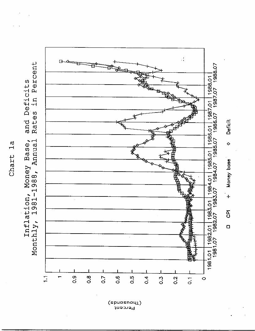
Chart 1a shows monthly percentage rates of change in prices, base money and deficit financing at annual rates for the period January 1981 to December 1988.3 The scale is in percent measured in thousands, so 1 is equivalent to 1000% and 0.1 is 100%. Including the years 1989 and 1990 compresses the data for the earlier years, so these years are shown separately in Chart 1 b where the scale runs from 0 to 11000%.

(Insert Charts 1a & 1b here) The period from 1986 to 1991 was characterized by several, sharp changes

in policy to bring down the rate of inflation. The details of these operations differed. A common feature is reliance on one-time changes to stop the momentum of inflation. Several plans used price and wage freezes. (Many prices in Brazil were controlled but indexed during the entire period.) One plan, the Cruzado plan, from March to October or November 1986 leaves a clear impression on Chart 1a. The measured rate of price change fell from an annual rate of 253% in February 1986 to 59% in December. By the following August, annual inflation reached a new peak, despite the introduction of a new plan - the Bresser plan - from May to August 1987.

The Verano plan in 1989 may have caused a slowing in the rate of inflation in the second quarter of that year, but any effect was short-lived. (Chart 1 b). By the end of the year, prices, base money and deficit finance accelerated to reach peak rates of growth above 6600%, 10,000%, and 4000% respectively.

Chart 1b makes clear that at the end of the price acceleration in 1989-90, base

3Ap/p, AB/B, A(B+S)/B+S each at annual rates from the same month of the preceding year.

10

(Ö

4-> U (0

o

co -P -H u

-H MH Q) Q

-ö a (d

4-> a o o u a) CM

c -H

co a) -p f0 t*

a) co (0 m

>1 a) c o S

G o

-H

(0 •H m G H

(Ö P Ö Ö

00 00 cr> rH

I rH 00 <T> rH

>1 rH

-P O S

(spuDsnoLLL) Q DJ

iH

-P u (d ü

CO -p

-p G (1) Ü M 0

-H CM Ü

G •H

-H 4-1 0) Q CO

0) TJ -P G «J 01 (Ú

(D (d co p (0 £ PQ G < >i

a o o <T> S CTv

\—I K I

G cr» o 00

-H CT» -P rH (Ö M-l G M ,G

•P G O S

en oo (O io to <N

(spuDsnoqjL) 3 DJ 3d

money growth exceeded the rate of inflation, and inflation exceeded the rate of increase of the deficit. Real balances were rising - a fact very different from the behavior for the period as a whole discussed earlier. Debt held by the public and deficit finance were rising more slowly than inflation; this, too, is opposite to the experience of the period as a whole, shown in Chart 1a.

The proximate cause of these changes was the inauguration of President Collor and the introduction of a new plan -- the Collor plan. This time prices and wages were not frozen, but a large part of existing financial assets, including portions of the public debt, was frozen for 18 months beginning in March 1990. Interest payments were accrued on these liabilities, so they no longer appeared in the cash budget and did not require current financing. Financial assets were taxed and tax payments accelerated. Hence, the Treasury reported a sharp reduction in the cash deficit for March and a surplus beginning in April. This reduced the size of new issues of base money and debt and brought the rate of inflation to an annual rate of 1600% by December. For the same period, deficit finance rose 400% and the monetary base rose by 2300%.

Current Inflation and Deficit Finance Recent annual rates of change overstate the current inflationary impulse by

including the earlier months of 1990 in the averages. An alternative measure of the current inflationary thrust may be the rates of change for the first quarter 1991 (from December to March), although this estimate includes the effects of the most recent price freeze instituted at the end of January 1991. Deficit finance rose by 30.7%, an annual rate of 122.8%. Base money increased by 143% (annual rate), well in excess of the target rate of 95%. If we assume that nominal GDP rises by approximately the rate of inflation and that "true" 1991 inflation is approximately equal to the growth rate of the base, 1991 GDP would be Cr $50, 943 million.* Deficit finance in the first quarter was Cr $1077, or Cr $4308 million at an annual rate. The ratio of the deficit

«Using 1990 preliminary GDP of Cr $ 35625 from Brazil Economic Program. March 1991, p. 17 times 1.43. Using the growth rate of the base abstracts from the price freeze and relies on the average relationship for 1985-90 shown in Table 1.

13

finance to GDP for 1991 computed in this way is 8.4%. This suggests that a conservative estimate of current deficit finance as a percent of GDP is about 8%.

The principal reason that the estimated deficit finance rate is described as conservative is that the budget does not include provision for financing of three major deferred charges: (1) the financial assets frozen by the Collor Plan due to be released beginning September 1991, (2) deferred payments to suppliers under the Collor Plan, and (3) interest payments on external debt. Rodriguez (1991, p. 21) estimates that the amounts outstanding in U.S. dollars are $27 billion, $10 billion, and $40 billion for each of these items, a total of $77 billion U.S. dollars.® In addition, there is the problem of financing the state governments by state bank borrowing. This problem has been deferred, not solved. The central bank has threatened to close the banks if they return to their expansionist policies, but this threat may be difficult to carry through.

To put the omitted interest payments into perspective, compare the interest payment on the $77 billion to the interest payments in the cash budget at the recent monthly nominal interest rate and exchange rate for March (14% on overnight BBC bonds and Cr $235 per dollar). The estimate is Cr $2533 billion of deferred interest compared to Cr $28 billion of interest expense in March 1991. (The latter is from Rodriguez op. cit. Table 3, p. 31

Rates of interest and rates of inflation in the early months of 1991 were broadly consistent with my estimate of government financing requirement, the growth of the monetary base, and uncertainty about future financing of deferred expenditures. Market participants appear to believe that inflation will continue at a rate in excess of 100% a year. For January and February, the average rate is about 20% per month.

An alternative estimate of Brazilian fiscal position is based on recent trends in

sCarlos Rodriguez, "Inflation in Brazil" The World Bank, May 1991 (xeroxed). Some of the financial assets have been released as a result of challenges to the government's authority to freeze assets. The releases to date do not require major adjustments in the calculation.

®l have not attempted to reconcile this table with the Rodriguez's Table 2, p. 20. 14

the government budget. Reported government spending increased at a compound annual rate of 141% for the 12 months ending January 1991,120% to February and 112% to March. This is a significant slowdown, given Brazil's rate of inflation. Government spending measured in U.S. dollars was 50% lower in March 1991 than a year earlier. These data are shown in Table 2.

Table 2 Total Government Spending in U.S. Dollars

1990 Total Spending Exchange Rate Total Spending Exchange Rate

Jan $10.6 14.3 September 4.6 75.6

Feb 8.6 24.4 October 43 95.0

March 73 37.8 November 4.1 126.5

April 45 48.7 December A3 158.7

1991

May 8.3 52.1 January 3 2 193.0

June 4.6 57.2 February 32 221.0

July 4.7 66.7 March 3.6 235.0

August 4.8 71.8

Source: Demonstrative da Execucao Financiera as reported in Rodriguez, op. dt- p. 31 col. 2, converted at exchange rates from col. 5 same source. Dollar expenditures are in billions.

Tax collections have slowed also during the period of the Collor plan, reflecting the sharp declines in output, income and spending in 1990. With real wages down by almost 25% in 1990, tax collections in U.S. dollars were lower by U.S. $2.6 billion from March 1990 to March 1991. Part of this decline reflects a one-time increase in revenues from acceleration of tax payments under the Collor Plan. Part is a one-time 7% tax on financial assets in March 1990. If we use the average tax collection for the third quarter as an approximation to the tax receipts that would be earned in an

15

expanding economy with rising real incomes, revenues would average about US $4.7 billion per month. With total spending held at US $3.5 billion, the budget would have a monthly surplus of US $1.2 billion before payment of the deferred interest and the unblocking of the accounts. This surplus, if achieved and sustained, would support annual interest payments and debt service of US $14 billion. This would be insufficient to service the US $77 billion of debt and obligations that has been omitted from the budget unless inflation and interest rates can be brought close to the levels in developed countries.

There are four problems with the alternative estimate. First, the budget numbers

from the Treasury report, which Rodriguez and I have used, do not reconcile with the

data on government financing (AB+AS) for the same period. If the budget surplus from April 1990 to March 1991 represented total government financing requirements, growth of base money and the government financing requirement should have been negative. Instead the base rose 490% in the first year of the Collor Plan (end of March 1990 to March 1991), and debt in the hands of the public rose 427% (after a decline of 70% at the start of the plan). Although the rate of increase of government financing slowed in the first quarter 1991, part of the improvement reflects the one-time effect of the price and wage freeze at the end of January 19917 The government appears to be financing a substantial amount of spending or outlays that is not included in the Treasury's budget report. Second, a wage and price freeze, introduced at the end of January, make the budget appear less expansive. Unless growth of money slows, wages and prices will increase rapidly when the freeze ends. The freeze distorts the underlying budget and financing. Third, the 1990 budget surplus was increased by special transactions, particularly the one-time reductions in interest payments, heavily negative real interest rates (a tax on debt) in March and April and the frozen payments

?For example, the Treasury reports a cash surplus of Cr $9.8 billion for first quarter 1991. Base money rose by 143% (annual rate) and the deficit by 123%. International reserves on the "liquidity" basis were approximately the same in April 1991 (US $8.8 billion) and March 1990 (US $8.7 billion) so the discrepancy is not explained by neglect of international reserve flows. Although reserves increased from March to August, they subsequently declined. The first quarter decline is US $1.3 billion.

16

to suppliers at the start of the Collor Plan. Fourth, many of the reductions in spending are more in the nature of postponements than cuts. This is a common problem, not unique to Brazil. Budget reduction often takes the form of reductions in spending on infrastructure or public investment. Schools, airports, roads, sewers and other capital projects to serve a growing population are deferred, not cancelled. Although such reductions help to bring the current budget into balance or reduce the current deficit, additional revenues (or other reductions) will be required in the future when the projects are reintroduced into the budget.

The inflationary potential arising from the gradual unfreezing of financial assets beginning in September 1991 can be reduced if the financial assets are exchanged for equity in state corporations and the money is retired. More generally, privatization of state assets offers a means of reducing government financing requirements and the stock of money. If government spending is tightly controlled while tax revenues increase (as the economy recovers), the one-time reductions of frozen and current money balances can produce a financing surplus and be used to reduce inflation permanently.

Preliminary Conclusion on Policy Brazilian policy for the past ten years has confused symptoms with causes and

relied on one-time stop gaps to temporarily reduce reported rates of price change. Examples abound. At different times Brazil's policymakers have introduced changes in the indexation formulas, periodic freezes on prices and wages, permanent or nearly permanent price controls, repeated changes in the currency unit, and in 1990 a freeze on a large part of the stock of financial assets. Some of these actions may have prevented hyperinflation, but they have not succeeded in stopping inflation or restoring Brazil to financial stability.

These stopgaps continue. In 1991, prices and wages were frozen again, and the market for overnight government securities was eliminated. The indexation formula was changed again by replacing the index based on past inflation (BTN) with a new index (TR) based on market interest rates. Whatever merit (or demerit) these measures may have, they do not constitute an anti-inflation policy.

17

Consider the recent decision to eliminate the overnight market in government securities. This market came into being in a period of variable inflation to encourage financial firms to hold government securities. The old system gave holders of overnight debt the option of putting their holdings to the government when interest rates rose without incurring a loss. The effect was to give a guarantee against short-term losses and shift the risk of loss from unanticipated increases in inflation to the government. The new decision returns the risk to the market. This is appropriate, long overdue, and should be welcomed. However, since Brazilian inflation remains highly variable, the market will charge the cost of risk bearing to the government. Real interest rates, already high relative to rates abroad, will include a premium for bearing this risk. If the new policy change was taken to improve control of money, by avoiding the requirement of repurchasing Treasury debt when inflation increases, it will succeed only if the government and the central bank are willing to pay the higher real interest rates that the policy requires. The key to success is a credible, sustained reduction in inflation and its variability.

Shifting, ad hoc, one-time policies have reduced the government's credibility. Since all past plans have failed to reduce inflation permanently, it would be surprising if the public could be convinced quickly that a future plan would succeed or be carried through. Uncertainty about future policy toward frozen financial assets, state banks, payments due to government suppliers, and privatization adds to the excess burden imposed by the lack of credibility. Any new effort to control inflation, if it is to succeed, must confront this entrenched skepticism.

Control of Money and Its Components

The necessary condition for controlling inflation is sustained, credible control of money. This discussion of monetary control has three aspects. First is control of the monetary base by the central bank. Second is the relation of the monetary base to other monetary aggregates, the various measures of money. Third, is the relation of money to nominal output or prices, usually discussed in terms of the demand for money or in terms of "causality" ~ whether the relation between money and nominal

18

aggregates reflects the effects of money on these aggregates or the converse. This section discusses the relation of the base to the monetary aggregates

during the past decade. Later sections consider the other topics. If the base is not related to the other monetary aggregates, the central bank

cannot control these monetary aggregates by controlling its balance sheet. Intermediation and disintermediation could disturb the relationship between base money and nominal GNP or prices and render control of the base useless for monetary control. A finding that this is not so does not establish that inflation can be controlled by monetary policy, but it removes intermediation as a source of disturbance in the relation of base money to output and prices.

Chart 2 shows monthly values of the money multipliers since 1980 for three definitions of money. These multipliers are computed as the ratio of a particular definition of money to the monetary base.

(Insert Chart 2 here) The chart makes clear that the multipliers for Mi, M3 and M4 moved differently.

The Mi multiplier is approximately constant. If the central bank controls the base, it controls Mi about as well. The multipliers for M3 and M4 show an upward trend during the decade of the 1980s that is interrupted by two strong reversals. The first, in 1986, coincides with the Cruzado plan. The second in 1990 coincides with the Collor plan. The freezing of deposits and other financial assets removed a significant fraction of deposits, raising the ratio of currency to total deposits. The rise in the ratio of currency to total deposits lowered the money multipliers for M3 and M4.8

Changes in the M3 and M4 multipliers initiated by the two plans were one-time changes. The 1986 reduction was clearly reversed in little more than a year; by June 1987, both multipliers were above the values in February 1986, just prior to the announcement of the plan. If M3 or M4 are the money measures most relevant for

8A complete framework and model of the interrelation of the stocks of money, base money, and the interrelation of banks, intermediaries and households is in Karl Brunner and Allan H. Meitzer, "Money Supply" in B. Friedman and F. Hahn, (eds.) Handbook of Monetary Economics. Amsterdam: North Holland, 1990, Chap. 9.

19

CO a o •H P •H £ -H

a) -o

CO P O

-H M (0 >

' O CT»

O) er» co (0 i

eg PQ o 00

•P U M rH (0 (0

-P >1 O 0) rH

C O -P S G

o <D S

-p

o -p

>1 a) G o S m o o

-H -P

to

prices, we see that the one-time reductions in the rate of price change in 1986 and 1990 were induced at least in part by the reductions in the money multipliers. If Mi, is the relevant concept, this is clearly not so; for Mi the 1986 changes

appear as a decline in velocity that also reversed in 1987. Charts 1a and 1b above show that the decline in the rate of price change clearly

preceded the decline in the rate of change of the base by several months in 1986 and by one month in 1990. Lower rates of price change and lower interest rates reduced government spending, the deficit financing requirement and the growth of the base. Hence, inflation fell before deficit finance and money growth.

The M3 and M4 multipliers capture more of the one-time effects of the policy

changes in 1986 and 1990. Given the size of the changes, it is not surprising that Rodriguez finds that these measures of money are more closely related to the measured rate of price change than either Mi or the monetary base.

The implication for inflation control is less clear. The failure to reduce the growth of the base in 1986 contributed to the acceleration of prices once the price freeze ended. The one-time changes in money and prices appeared to lower inflation, but this was a mirage. The mirage did not mislead the public; they increased spending to take advantage of the price freeze. In this, they were encouraged by the continued expansion of the base. The result was renewed inflation at a higher rate in 1987.

The relation between base money growth and rates of price increase in 1986 is inverse; faster base growth coincides with a lower rate of price change in 1986, and conversely in 1987. The data are shown in Table 3.

For the two years, 1986 and 1987 together, the two rates are relatively close. Lest this be considered accidental, recall from Table 1 that the close relation holds for the period as a whole, and note that for 1985 the two rates of increase are also close, 257 and 239. For comparison, Table 3 also shows the growth rate of debt held by the public. Together, the movements of debt and money show that the plan did not produce a permanent decline in the government financing requirement.

Aside from the relatively large policy-induced changes in 1986 and 1990 all three multipliers appear stable. Clearly the Mi multiplier is the most stable of the three,

21

Table 3 Percent Rates of Increase in Base Money and Prices,

1986 and 1987

1986 1987 Mean

Base Money 293 182 238

Prices (INPC) 59

396 228

Debt 39

531 285

but the M3 and M4 multipliers appear to have a predictable trend and seasonal

component, especially in the years prior to 1986. Fluctuations in the multipliers and their trend can be examined further by

looking at the components of the multipliers. The components can be written as ratios, for example the ratio of currency to deposits, the ratio of time and saving deposits to demand deposits and the ratio of reserves to some measure of deposits. Two of these ratios are shown in Charts 3a and 3b.

The ratios in Charts 3a and 3b move inversely to each other, and their relative movements, measured as percentage rates of change, are of similar order of magnitude. It is easily shown that both increases in the ratio of currency to total deposits (chart 3a) and increases in the ratio of time and savings deposits to demand deposits (chart 3b) lower the Mi multipliers Since the two ratios have moved in opposite directions, their effects on the Mi multiplier have been offsetting. This contributed to the stability of the Mi multiplier. Moreover, the monthly value of this multiplier can be predicted with reasonable accuracy. An autoregressive estimate

9Provided the reserve ratio (1) is less than one, as is true for Brazil. Let Mi = C+D and the base, B=R+C, where C is currency, D is demand deposits, and R is reserves. Let T- the sum of time and saving deposits. Assume C=k(D+T), R = r(D+T) and T=tD, r, t and k can depend on other variables such as inflation or, in the case of t, relative interest rates. Then the Mi multiplier is mi = 1+fc(1+<)/[(r+/c)(1+<)]. Differentiating gives the result in the text.

(Insert Charts 3a & 3b here)

22

based on data for March 1980 to December 1990 shows that 73% of the variance of the monthly Mi multiplier is explained by the multiplier lagged once, so forecasting the

multiplier would have posed little problem. The movements of the currency and time deposit ratios are not offsetting for M3

and M4. Increases in the ratio of time and savings deposits to demand deposits reduce the Mi multiplier but raise the multipliers of M3 and M4. Increases in the currency ratio lowers these multipliers, so the inverse correlation of the two ratios implies that movements of the two ratios typically reinforce one another in their effect on these multipliers. Changes in the multipliers are dominated by the changes in the two ratios. The freezing of demand deposits in 1990 and their removal from the deposit stocks, therefore, had little effect on the Mj multiplier but dramatic effects on the currency and time and saving deposit ratios and, thus, on the M3 and M4 multipliers.

Rodriguez shows a rise in the ratio of currency to demand deposits beginning in 1987. (His Figure 6). He interprets the rise as evidence of a shift by firms out of demand deposits to avoid the inflation tax. He writes: "In high inflation, firms are better positioned to avoid the inflation tax then individuals."") Chart 3a shows that the inference is not warranted if we define the currency ratio to include total deposits in the denominator. The use of currency declined relative to total deposits; individuals and firms shifted into interest bearing deposits to avoid some of the inflation tax.

Monetary Velocity

A common observation in countries experiencing inflation is that money balances per unit of income fall. Inflation is a tax on money holding that induces holders to accept the inconvenience of lower real money balances per unit of real income. In the language of taxation, the tax base declines as the tax rate increases.

Brazil has encouraged indexation of interest payments on financial assets and

lORodriguez, op. cit.. p. 23. 25

has issued indexed government securities with guaranteed real returns. Indexation compensates, in whole or part, for the inflation tax. Throughout the period of high or rising inflation, Brazilians were able to hold financial assets in indexed form. Charts 3a and 3b above showed the shift of financial assets from assets with non-indexed returns - currency and demand deposits - to assets with indexed returns - time and saving deposits. Government securities and money market accounts also increased absolutely and relative to assets with non-indexed returns.

Chart 4 shows three measures of monetary velocity, defined as the ratio of

nominal GDP to money. From previous charts, we know that movements of M3 and M4

are highly correlated, so I have omitted the velocity of M3. Chart 4 shows that the

velocities of M2 and M4 move concurrently and in the same direction. Movement of the

velocity of M2 and M4 is dominated by negative trends; these measures of velocity

decline on average until 1989. Both rise sharply in 1990 as a consequence of the

freezing of financial assets that lowered the denominator of the ratio. (Insert Chart 4)

The trends in M2 and M4 velocity are opposite to the trends expected under rising inflation if both movements were dominated by the inflation tax. Indexation appears to have succeeded in avoiding a flight from money and financial assets in Brazil.

Mi velocity shows two periods of rising trends broken by a sharp fall in 1986.

This is the counterpart of the rapid growth of base money and M^ in 1986 during the

price freeze instituted as part of the Cruzado plan. Inflation in Brazil began long before 1980. Flight from money may have

occurred before the start of the data series used here. To consider this possibility, Table 4 compares Brazilian GDP velocity to measures of velocity for the United States and Chile. The United States has a well developed financial system, low inflation compared to Brazil, but little formal indexation. The use of financial instruments is widespread. Chile has experienced rapid inflation that has now slowed to a more moderate range. Its financial system is less indexed than Brazil's. The definition of M1 is more nearly uniform across countries than definitions of the broader aggregates, so I

26

Table 4 Comparative Measures of Velocity

Brazil 1981 Brazil 1989 Chile 1988 United States 1990 Mi 8.8 12.3 16.9 6.6

have used Mi velocity for Chile, the United States and Brazil. Table 4 suggests that Mi velocity in Brazil is intermediate between Chile and

the United States. These data give no evidence of a flight from money in Brazil. On the contrary, the movements of velocity are relatively small, considering the rate of inflation and the frequent shifts in policy during these years. Annual deviations of Mi velocity from its mean for the period never exceed 30% and generally are much smaller.

The coefficient of variation if a commonly used measure of variability relative to the mean value. Table 5 shows the coefficient of variation for four measures of monetary velocity computed from annual data for 1980-89 inclusive. I have omitted 1990 because of the large change in velocity resulting from the freeze on financial assets.

Table 5 Variability of Annual Velocity, 1980-89 V̂ V2 V3 V4

Coefficient of Variation 0.17 0.32 0.32 0.32

The data confirm the impression given by inspection of Chart 4. The variability of velocity was not a significant deterrent to monetary control. The values in Table 5

28

contrast sharply with the coefficients of variation of inflation (INPC) and base money growth for the same period-1.29 and 1.34 respectively. The comparison suggests that inflation would have been stopped permanently if Brazil had established procedures capable of controlling the government financing requirement and money growth.

From Table 1, we know that the compound annual rate of inflation was more than 150% from 1981 to 1990 and more than 200% in the last part of the decade. Average annual inflation rates were far in excess of these numbers, almost 600% from 1985 to 1990. Clearly, changes in velocity were not a principal disturbing factor in inflation control. This conclusion based on annual data supports the similar conclusion based on estimates of the demand for real money balances in Rodriguez, QP, Cit,

Rodriguez uses monthly data for the five years January 1985 to December 1989 in his estimates of the demand for money. Based on these estimates and his study of money supply, he concluded that M4 was the most reliable aggregate for monetary control.

The results he presents are not as clearcut as the conclusion he draws. The demand for money equations are estimated from monthly data for a brief, and turbulent, period. The equations do not include the own yield on money, a matter of some importance in the context of Brazil where indexation kept the own yield on M2, M3, or M4 very close to the market rate or the rate of inflation. The regressions show that the measure of output (log PBI) has a coefficient near to unity and not significantly different from unity for M3, M4, and M4-TF. Hence these measures of velocity should remain approximately constant in the absence of changes in interest rates or inflation or, in the case of M4, perhaps rise on average. The relatively large estimated interest elasticities suggest that, as inflation and interest rates rose, real money balances declined. Hence, velocity should rise with inflation, particularly M4 velocity. We know from Chart 4 that M4 velocity declined on average during this period to 1989. The omission of the indexed return to M4 balances may have biased the estimates of the coefficients or put the response to the own rate into the trend that Rodriguez incorporated in the moving average. Whatever the facts may be, I believe that the

29

relatively large interest rate or inflation elasticity is misleading. It suggests a reduction in real money balances contrary to the evidence on money and prices.

The important issue for Brazil is not whether they must choose one or another monetary aggregate to control on a monthly or quarterly basis. What matters for Brazil is evidence showing that Brazil's inflation is principally caused by money creation, not by a flight from money and a rise in velocity. Whatever may have happened in a particular year as a result of policy shifts or random events, the trends in velocity in Tables 1 or 4 or in Chart 4 and the measures of variability in Table 5 are sufficient to make this point: velocity was not a principal source or even an important source of inflation. For the broader aggregates, the trend in velocity made a modest contribution to lower inflation. The last conclusion is, of course, the same as the conclusion reached in the discussion of Table 1.

In countries where velocity falls during inflation, average real cash balances reach relatively low levels. The end of inflation induces transactors to replenish real money balances. The demand for money increases and velocity falls. Some central banks anticipate this response of real balance by maintaining money growth in excess of the growth of nominal GDP during the transition to low inflation.

Since Brazil has not experienced any sizeable internal flight from money, it should not expect a large increase in the demand for money if inflation is reduced to zero, to the level of the early 1970s, or to the current level of Chile or Mexico.

Causality

The remaining issue about the relation of money to inflation is the cause of the Brazilian inflation. This issue is often posed by asking: Is money growth the cause of Brazilian inflation?

To answer this question, Rodriguez, op. cit.. tests for Granger causality. He compares the lagged effect of measures of money growth on inflation to the lagged effects of inflation on money growth using filters to remove trends. Rodriguez does not put much weight on the answer, but his findings show a stronger relation from prices to

30

money than from money to prices. 11 I believe these causality tests ask the wrong question and give the wrong

answer. Consider three examples used earlier. First, consider the oil shock of 1979-80. Prices rose. Under Brazilian indexation, the budget deficit increased and money growth rose to finance the deficit. Hence, the timing of the changes went from prices to money. Under Brazilian institutions, the rise in inflation was unavoidable following a real shock. Second, a similar argument applies to the so-called real devaluation of 1980. Import prices accelerated before money growth increased, so inflation led and money growth followed. Third, in 1986 a price freeze lowered the measured rate of price change. The base continued to rise at a rapid rate. When the price freeze ended, prices accelerated; for the two years as a whole, the average rate of price change and the average rate of base growth (or Mi growth) are about equal. The price freeze altered the timing but not the magnitude of the relation. In a test of Granger causality, timing is critical. For 1966, the price freeze distorts the timing relationship. Since the movements of prices and money are large in this period, the distortion affects the estimates, particularly for Mi and the base.

As Schwert has shown, Granger causality is a particular form of causality that is better described as "temporal precedence."^ A variable is said to be causal if it moves earlier. I do not believe that this is the meaning of causal most relevant for the discussion of inflation.

Two issues are more relevant for causality. First, is money growth necessary (or necessary and sufficient) for inflation, and are changes in money growth necessary for proportional changes in the rate of inflation? Second, can money growth be controlled?

Define inflation as the maintained rate of price change. Since velocity growth contributed little to the inflation of the 1980s, money growth has been the source of

11 For reasons given below, I do not comment on the technical details.

12G. William Schwert, "Tests of Causality" Carnegie-Rochester Conference Series on Public Policy, 10,1979, pp. 55-96.

31

inflation. When money growth was lower, inflation was lower, and when money growth rose, inflation rose. Maintained inflation excludes one-time price changes that can have non-monetary causes. But the one-time price changes became maintained rates of price change in Brazil, if and only if money growth increased.^ In this sense, which I believe is the relevant sense, money growth is causal even if the timing relation shows that price changes precede changes in money growth at times or on average.

Institutional arrangements can prevent or hinder central bank control of money growth. An example is a fixed exchange rate system, such as the Bretton Woods system. Under the Bretton Woods system, each member country maintained a fixed exchange rate against the dollar. The United States controlled the rate of change of money. When U.S. money growth increased, member countries had to choose between revaluation of their currencies or inflation. If they kept exchange rates fixed, their domestic money growth and rate of inflation increased with U.S. money growth. Inflation was caused by money growth, but inflation and money growth could not be controlled outside the U.S. under the prevailing institutions.

A second example is closer to current Brazilian experience. During the 1970s, the Italian government ran relatively large budget deficits and issued debt to finance the deficits. Under prevailing arrangements, the Bank of Italy was responsible for purchasing all the bonds not sold in the market at a given rate of interest. The rate of interest was not allowed to rise to clear the bond market, so the Bank of Italy issued base money. The growth of the base was the proximate cause of inflation, but inflation could not be controlled under the prevailing arrangement. Eventually, the arrangement was abandoned and the rate of inflation was reduced.

Brazil ran relatively large deficits and deficit finance rose throughout the 1980s. During this period, nominal interest rates were not allowed to rise enough to clear the market for securities. There was no futures market in which bond owners could hedge the risk of changes in the rate of inflation. Instead, the central bank chose as its target

i3Let (1 /p)(dp/df) = k + Ap where dp/p is the rate of price change, k is the rate of inflation (maintained rate of price change) and Ap is a one-time change in price level.

32

the ex-post rate on government securities (LFT during the run-up to hyperinflation in 1989-90). The aim was to guarantee a real return that would induce the market to hold the government's debt and acquire its new issues.

When inflation rose, the market put securities to the central bank. An unanticipated rise in inflation, therefore, required the central bank to buy securities and issue base money. In a temporal sense, inflation led the rate of money growth.

Inflation could only be stopped under this arrangement by raising ex post real rates high enough to induce the market to hold the debt. The government, or the central bank, did not consider this an acceptable solution. As is often the case, the real rate of interest eventually rose far beyond the rate that would have stopped the inflation in the 1970s or prevented the hyperinflation at the end of the 1980s. The real rate eventually reached levels that produced major recessions without stopping the inflation.

Institutional arrangements have been changed to give greater scope for monetary control, but it does not appear that an adequate system is in place. Brazil has again found it necessary in 1991 to freeze prices and wages and to make other ad hoc changes to prevent a new rise in inflation.

What Should Be Done?

Brazil faces three problems in implementing a system of monetary control to end inflation. First, much progress has been made in reducing the real level of government spending, but the government financing requirement rose at an annual rate of 125% in the first quarter, despite the price and wage freeze and other actions at the end of January. Second, decades of ad hoc, intermittent measures and failure of successive plans has reduced credibility. High real rates of interest suggest a large premium for uncertainty and skepticism about the future. Third, there should be concern for what would happen if disinflation succeeded.

Fiscal control, particularly control of the financing requirement, is the essential first step toward credibility, reduced uncertainty and lower interest rates. If uncertainty and real interest rates could be reduced, real growth would return. This would raise

33

government revenues and produce a surplus provided government spending remains tightly controlled. But, nominal and real rates of interest cannot be reduced until there is a credible anti-inflation program. And a credible program will not be sustained without major reduction in the financing requirement. How can the Brazilian government break into this interdependent set of problems?

I propose that the government take a bold step to restore its credibility by closing the monetary operations of the central bank.™ In its place, Brazil would establish a currency board, modelled on the monetary systems in Hong Kong, Singapore, Panama and some other countries. The nominal exchange rate for the cruzeiro would be pegged to the U.S. dollar. Commercial banks would issue cruzeiros only in exchange for convertible foreign money at prevailing exchange rates. A loss of foreign exchange would require the banks to reduce cruzeiros commensurately. Since the monetary base was less than U.S. $7 billion and Mi was about U.S. $10 billion at the end of December 1990, Brazil has sufficient international reserves to implement this system. All new issues of money would be backed 100% by foreign currency.

Adopting a credible currency board system would have five major effects: (1) inflation would fall to about the U.S. level; (2) nominal interest rates would fall to about the U.S. level, or slightly above; (3) interest payments would fall substantially, lowering budget expenditures; (4) government deficits could only be financed from domestic saving and

foreign capital, so spending would be controlled; (5) Brazil would lose the small inflation tax revenues that it currently receives

but would continue to collect seigniorage on outstanding currency.

A necessary step to make the system work would be reduction in the government financing requirement. In a previous section, I estimated that this could be achieved if real spending remained close to its current level, U.S. $3.5 billion per month as the economy recovered and recovery increased tax revenues toward US $5

^Supervisory and other non-monetary activities would continue. 34

billion per month realized early in the current recession (third quarter 1990). The main forces for recovery would be the reduction in uncertainty about future

inflation, the decline in nominal and real interest rates, and the strength of Brazilian exports. The latter have been sustained through most of the years of high inflation. Reduction in uncertainty would encourage higher investment and more long-term investment, encouraging progress and development.

To maintain credibility, the budget would have to produce a surplus sufficient to service outstanding debt and pay interest and amortization on frozen financial assets and deferred business claims on the government. This debt consists (at the end of March 1991) of Cr $8700 billion of deferred claims. At a 15% nominal interest rate (assuming a credible currency board is in place), the annual interest payment on these claims would equal between one and two month's tax revenue at the rate of third quarter 1990. Additional interest payments would be required on the international debt.

The budget position appears to be consistent with a currency board system if real spending can be held near its current level and revenues restored to the pre-recession level. More detailed knowledge of the Brazilian fiscal system is required to reach a firm conclusion on these points.

Rapid disinflation is likely to follow adoption of a credible, currency board. Extensive indexation of the Brazilian economy would buffer the system against much of the shock of rapid disinflation. I am uncertain about one, particularly important, risk arising in disinflation - the risk to banking and financial institutions.

The risk arises in many countries from the role of land as a relatively profitable asset to hold in periods of inflation and the widespread practice of using land as collateral for loans from financial institutions. Today's land prices incorporate an estimate of future inflation. If inflation falls and is expected to remain low, land prices will decline markedly reflecting the lower anticipated rate of inflation. Banks and financial institutions could find that the value of the assets underlying property loans and mortgages declines so rapidly that borrowers default, causing widespread losses for financial institutions and failures of financial firms. Government would be called upon to prevent these failures by assuming large claims. Financing these losses

35

could lower the credibility of the program. Brazil's system of indexation may be sufficient to reduce this risk or avoid it. I am not sufficiently familiar with the detail to know.

If these concerns about budget finance and the prevention of widespread financial system failures are satisfied, I believe credibility can be restored and inflation reduced to about the U.S. rate by adopting a currency board.

36

Appendix

Velocity Computed from End of Year Data (EOY) and Annual Averages (AVG)

Year EOY AVG EOY AVG EOY AVG

1980 8.9 12.2 6.3 8.2 3.6 4.6

1981 8.8 13.6 5.0 7.8 2.8 4.2

1982 11.6 15.4 5.5 7.5 2.8 3.8

1983 12.8 19.2 6.3 8.8 2.5 3.9

1984 13.9 25.9 4.8 9.5 2.1 3.8

1985 12.4 26.2 3.7 6.9 1.9 3.3 1986 8.0 12.0 4.5 5.6 2.6 3.1 1987 11.1 21.0 3.5 6.6 1.8 3.3 1988 12.4 33.9 2.6 7.3 1.2 3.4 1989 12.3 45.8 1.8 6.5 1.1 3.7

1990 14.1 30.6 8.1 14.7 3.8 7.4

Averages are yearly averages of monthly data.

37