Innovation and Top Income Inequality∗†

Philippe Aghion Ufuk Akcigit Antonin Bergeaud

Richard Blundell David Hemous

February 23, 2018

Abstract

In this paper we use cross-state panel and cross-US commuting-zone data to look atthe relationship between innovation, top income inequality and social mobility. We findpositive correlations between measures of innovation and top income inequality. Wealso show that the correlations between innovation and broad measures of inequalityare not significant. Next, using instrumental variable analysis, we argue that thesecorrelations at least partly reflect a causality from innovation to top income shares.Finally, we show that innovation, particularly by new entrants, is positively associatedwith social mobility, but less so in local areas with more intense lobbying activities.

JEL classification: O30, O31, O33, O34, O40, O43, O47, D63, J14, J15

Keywords: top income, inequality, innovation, patenting, citations, social mobil-ity, incumbents, entrant.

∗Addresses - Aghion: College de France, London School of Economics and CIFAR. Akcigit: Universityof Chicago, CEPR, and NBER. Bergeaud: Banque de France. Blundell: University College London andInstitute of Fiscal Studies. Hemous: University of Zurich and CEPR.†We thank Daron Acemoglu, Pierre Azoulay, Raj Chetty, Lauren Cohen, Mathias Dewatripont, Peter

Diamond, Thibault Fally, Maria Guadalupe, John Hassler, Elhanan Helpman, Chad Jones, Pete Klenow,Torsten Persson, Thomas Piketty, Andres Rodriguez-Clare, Emmanuel Saez, Stefanie Stantcheva, ScottStern, Francesco Trebbi, John Van Reenen, Fabrizio Zilibotti, seminar participants at MIT Sloan, INSEAD,the University of Zurich, Harvard University, The Paris School of Economics, Berkeley, the IIES at StockholmUniversity, Warwick University, Oxford, the London School of Economics, the IOG group at the CanadianInstitute for Advanced Research, the NBER Summer Institute, the 2016 ASSA meetings and the CEPR-ESSIM 2016 meeting, and finally the referees and editor of this journal for very helpful comments andsuggestions.

1

1 Introduction

It is widely acknowledged that the past decades have experienced a sharp increase in top

income inequality – particularly in developed countries.1 Yet, no consensus has been reached

as to the main underlying factors behind this increase. In this paper we argue that, in a

developed country like the US, innovation is certainly one such factor. For example, in the

list of the wealthiest individuals per US state, compiled by Forbes Magazine, 11 out of 50 are

listed as inventors of a US patent and many more manage or own firms that patent. This

suggests these individuals have earned high incomes over time in relation to innovation. More

importantly, patenting and top income inequality in the US and other developed countries

have followed a parallel evolution. Thus, Figure 1 shows the number of granted patents and

the top 1% income share in the US since the 1960s: Up to the early 1980s, neither variable

exhibits a trend, but since then both variables experience parallel upward trends.

More closely related to our analysis in this paper, Figure 2 examines the relationship

between the increase in the log of innovation in a state between 1980 and 2005 (measured

here by the number of citations within five years after patent application, per inhabitant in

the state), and the increase in the share of income held by the top 1% in that state over the

same period. We see a significantly positive correlation between these two variables.

That the recent evolution of top income inequality should partly relate to innovation,

should not come as a surprise. Indeed, if the increase in top income inequality has been

pervasive across occupations, it has particularly affected occupations that appear to be

closely related to innovation such as entrepreneurs, engineers, scientists, as well as managers.2

We first develop a Schumpeterian growth model where growth results from quality-

improving innovations that can be made in each sector, either by the incumbent or by a

potential entrant. Facilitating innovation or entry increases the entrepreneurial share of in-

come and spurs social mobility through creative destruction. The model predicts that: (i)

entrants’ and incumbents’ innovation increase top income inequality; (ii) entrants’ innovation

increases social mobility; (iii) entry barriers lower the positive effects of entrants’ innovations

on top income inequality and social mobility. Yet, higher mark-ups for non-innovating in-

cumbents can lead to higher top income inequality and lower innovation.

We start our empirical analysis by exploring correlations between innovation and various

measures of inequality using OLS regressions. Since our innovation measures build on patent

data, we focus on appropriated innovation which is more likely to affect income inequality.

Our results can be summarized as follows. First, the top 1% income share in a given state

1Piketty and Saez (2003) documents the sharp increase in top income inequality in the US, while bookssuch as Goldin and Katz (2009), Deaton (2013) and Piketty (2014) have spurred a worldwide interest forincome and wealth inequality.

2Bakija et al. (2008) find that the income share of the top 1% in the US has increased by 11.2 percentagepoints between 1979 and 2005, out of this amount, 1.02 percentage points (that is 9.1% of the total increase)accrued to engineers, scientists and entrepreneurs. Yet, innovation also affects the income of managers andCEOs (Frydman and Papanikolaou, 2015), and firm owners (Aghion et al., 2018).

2

in a given year, is positively and significantly correlated with the state’s rate of innovation.

Second, innovation is less positively, or even negatively, correlated with broader measures

of inequality which do not emphasize top incomes, like the Gini coefficient, as suggested by

Figure 3. Next, the correlation between innovation and the top 1% income share weakens at

longer lags. Finally, it is dampened in states with high lobbying intensity.

To make the case that the correlation between innovation and top inequality at least

partly reflects a causal effect of innovation on top incomes, we instrument for innovation us-

ing data on the United States Senate Committee on Appropriations (following Aghion et al.,

2009). We argue that the composition of the appropriation committee affects the allocation

of earmarks across all states, and in turn affects patenting and innovation in the states. We

then regress top income inequality on innovation instrumented by the composition of the

appropriation committee. All the main OLS results are confirmed by the corresponding IV

regressions. Our IV results imply that an increase of 1% in the number of patents increases

the top 1% income share by 0.2%, and the effects of a 1% increase in the citation-based mea-

sures are of comparable magnitude. We also build a second instrument for state innovation

which relies on knowledge spillovers from other states. Although the two instruments are

uncorrelated, we find very similar effects.

Next, we calibrate the main parameters of the model with our regression results, and

use our calibrated model to reproduce the regressions of the paper. We find a very good

fit between the OLS and IV regressions coefficients on the one hand, and the coefficients

estimated from the calibrated model on the other hand.

Finally, we analyze the relationship between innovation and social mobility using cross-

sectional regressions at the commuting zone (CZ) level. We find that: (i) innovation is

positively correlated with upward social mobility (as suggested in Figure 4); (ii) this corre-

lation is driven by entrant innovators, and dampened in CZs with high lobbying intensity.

The analysis in this paper relates to several strands of literature. First, we contribute

to the endogenous growth literature (Romer, 1990; Aghion and Howitt, 1992; Aghion et al.,

2014; Akcigit, 2017) by looking explicitly at the effects of innovation on top income shares

and social mobility.

Second, our work adds to the empirical literature on inequality and growth (see for

instance Barro, 2000 who studies the link between overall growth and inequality measured

by the Gini coefficient, Forbes, 2000 or Banerjee and Duflo, 2003). More closely related to

our analysis, Frank (2009) finds a positive relationship between both the top 10% and top

1% income shares and growth across the United States. We contribute to this literature by

showing that innovation-led growth is a source of top income inequality.

Third, a large literature on skill-biased technical change aims at explaining the increase

in labor income inequality since the 1970s.3 While this literature focuses on the direction of

3Katz and Murphy (1992) and Goldin and Katz (2009) have shown that technical change has beenskill-biased in the 20th century. Lloyd-Ellis (1999), Acemoglu (1998, 2002) or Hemous and Olsen (2016)

3

innovation and broad measures of labor income inequality (such as the skill-premium), we

focus on the rise of the top 1% and its relation with the rate of innovation.

Fourth, our paper relates to recent literature on inequality and firm dynamics. Rosen

(1981) emphasizes the link between the rise of superstars and market integration: namely, as

markets become more integrated, more productive firms can capture a larger income share,

which translates into higher income for their owners and managers. Similarly, Gabaix and

Landier (2008) show that the increase in firm size can account for the increase in CEO’s pay.

Song et al. (2015) show that most of the rise in earnings inequality can be explained by the

rise in across-firm inequality rather than within-firm inequality. Our analysis is consistent

with this line of work, to the extent that successful innovation is a main factor driving

differences in productivity across firms, and therefore in firms’ size and pay.4

Finally, worthy of mention is a new set of papers on innovation and individuals’ income.

Frydman and Papanikolaou (2015) find that innovation and executive pay are positively

correlated (Balkin et al., 2000 find the same result in high-tech industries). Aghion et al.

(2018) use data from Finland to show that innovation increases an individual innovator’s

probability to make it to the higher income brackets, and innovation has an even larger

effect on firm owners’ income. Bell et al. (2016) find that the most successful innovators see

a sharp rise in income. Akcigit et al. (2017) find a positive correlation between patenting

intensity and social mobility across the United States over the past 150 years.

Most closely related to our paper, Jones and Kim (2017) also develop a Schumpeterian

model to explain the dynamics of top income inequality. In their model, growth results

from both the accumulation of experience or knowledge by incumbents (which could result

from incumbent innovation), and creative destruction by entrants. The former increases top

income inequality whereas the latter reduces it.5 In our model instead, a new (entrant)

innovation increases mark-ups in the corresponding sector, whereas in the absence of a

new innovation, mark-ups are partly eroded as a result of imitation. Both papers have in

common: (i) that innovation and creative destruction are key factors in the dynamics of top

income inequality; (ii) that fostering entrant innovation contributes to making growth more

“inclusive”.6

The remainder of the paper is organized as follows. Section 2 outlays a Schumpeterian

endogenize the direction of technical change. Krusell et al. (2000) relate the increase in the skill premiumwith the increase in the equipment stock. Several papers (Aghion and Howitt, 1998; Caselli, 1999 and Aghionet al., 2002) argue that General Purpose Technologies increase labor income inequality.

4Our analysis is also consistent with Hall et al. (2005), Blundell et al. (1999) or Bloom and Van Reenen(2002) who find that innovation has a positive impact on market value.

5In Jones and Kim (2017) entrants innovation reduces income inequality because it affects incumbents’efforts so that an exogenous increase in entrant innovation affects inequality only if it is anticipated byincumbents. Moreover, their model predicts a positive correlation between growth and inequality in theshort-run (due to a scale effect) and a negative correlation only in the long-run.

6Indeed, we show that entrant innovation is positively associated with social mobility. Moreover, whilewe find that incumbent and entrant innovation contribute to a comparable extent to increasing the top1% income share, additional regressions in Table C1 of Appendix C suggest that incumbent innovationcontributes more to increasing the top 0.1% or top 0.01% than entrant innovation.

4

model to guide our empirical analysis. Section 3 describes our state panel data on inequality

and innovation. Section 4 presents our OLS results. Section 5 explains our IV instrument and

shows our IV results. Section 6 reports robustness tests. Section 7 performs our calibration

exercise. Section 8 looks at the relationship between innovation and social mobility. Section

9 concludes. An online appendix with additional theoretical and empirical results, and a

more detailed description of the data and the calibration, can be found at this link.

2 Theory

In this section we develop a simple Schumpeterian growth model to explain why increased

R&D productivity increases both the top income share and social mobility.

2.1 Baseline model

We consider a discrete time economy populated by a continuum of individuals of measure M .

At any point in time a mass M/(1+L) of individuals are firm owners and the rest, ML/(1+

L), are workers (so L ≥ 1 is the ratio of workers to entrepreneurs). Each individual lives

for one period. Every period, a new generation is born and individuals born to current firm

owners inherit the firm from their parents. The rest of the population works in production

unless they successfully innovate and replace incumbents’ children.

2.1.1 Production

A final good is produced according to the following Cobb-Douglas technology:

lnYt =

∫ M/(1+L)

0

1 + L

Mln yitdi, (1)

where yit is the amount of intermediate input i used for final production at date t. The

number of product lines M/(1 + L) scales up with population size (as in Howitt, 1999).

Therefore, the final good sector spends the same amount, Yt, on all intermediates:

pi,tyit = Yt =1 + L

MYt for all i. (2)

Each intermediate i is produced by a monopolist who faces a competitive fringe, using a

linear production function:

yit = qitlit, (3)

where lit is the amount of labor hired to produce i at t, and qit is labor productivity.

5

2.1.2 Innovation

Productive innovation Whenever there is a new “productive innovation” in any sector

i in period t, quality in that sector improves by a multiplicative term ηH > 1 so that:

qi,t = ηHqi,t−1.

In the meantime, the previous technological vintage qi,t−1 becomes publicly available, so that

the innovator in sector i obtains a technological lead of ηH over potential competitors. Both

entrants and incumbents can undertake productive innovations. We denote their respective

productive innovation rates by xE,i and xI,P,i in line i. At the end of period t, other firms

can partly imitate the (now incumbent) innovator’s technology so that, in the absence of

a new innovation in period t + 1, the technological lead enjoyed by the incumbent firm in

sector i shrinks from ηH to ηL with 1 < ηL < ηH .

Defensive innovation The incumbent may instead undertake a “defensive innovation”

which does not increase productivity (i.e. qi,t = qi,t−1) but ensures maintaining a technolog-

ical lead of ηH . That is, a defensive innovation prevents potential competitors from using a

technology which is too close to the incumbent’s. We denote by xI,D,i the defensive inno-

vation rate of incumbents. Again, in the absence of a new innovation in period t + 1, the

technological lead of the incumbent shrinks back to ηL.

Overall, the technological lead enjoyed by the incumbent producer in any sector i takes

two values: ηH in periods with innovation and ηL < ηH in periods without innovation.7

To innovate with probability xE,i a potential entrant needs to spend

CE,t (x) ≡θEx

2E,i

2Yt;

while to undertake productive innovation at rate xI,P,i and defensive innovation at rate xI,D,i,

an incumbent needs to spend

CI,t (x) ≡ θI (xI,P,i + xI,D,i)2

2Yt.

The parameters θE and θI capture R&D productivity for entrants and incumbents respec-

tively, and the innovation cost functions scale up with per capita GDP.

Introducing the dichotomy between productive and defensive innovations allows us to

capture the difference between patents and “true innovation”: namely, some patents are

used to protect rents without contributing much to productivity growth. Indeed, a growing

number of defensive patents may explain why the observed increase in patenting does not

7 The details of the imitation-innovation sequence do not matter for our results, what matters is thatinnovation increases the technological lead of the incumbent producer over its competitive fringe.

6

seem to be fully reflected in productivity growth.8

Finally, we assume that an incumbent producer who has not recently innovated, can still

resort to lobbying in order to prevent entry by an outside innovator. Lobbying is successful

with exogenous probability z, in which case the innovation is not implemented and the

incumbent remains the technological leader in the sector (with a lead equal to ηL).

2.1.3 Timing of events

For simplicity, we rule out the possibility that both entrant and incumbent innovate in the

same period.9 We also assume that in each line i a single potential entrant is drawn from

the mass of workers’ offspring. The timing of each period is summarized in Figure 5.

2.2 Solving the model

To solve the model, we first compute the entrepreneurs’ and workers’ income shares and the

rate of social mobility at given innovation rates. We then endogeneize innovation.

2.2.1 Income shares and social mobility for given innovation rates

In this subsection we assume that in all sectors, at any date t, potential entrants innovate

at some exogenous rate xEt and incumbents innovate at some exogenous rate xIt, knowing

that a share φt of their innovations is productive. Limit pricing in any intermediate sector i

implies that the price charged by the incumbent producer is equal to the technological lead

ηit times the marginal cost MCit = wt/qi,t, hence:

pi,t = wtηit/qi,t, (4)

where ηi,t ∈ {ηH , ηL}. Innovation allows the technological leader to (temporarily) increase

the mark-up from ηL to ηH .

Equations (2) and (4) allow us to express equilibrium profits in sector i at time t as

Πit = (pit −MCit)yit =ηit − 1

ηitYt.

Thus equilibrium profits only depend upon mark-ups and aggregate output. Profits are

higher whenever the technological leader has recently innovated (no matter the type of

8An alternative or complementary explanation is that productivity growth from creative destruction maybe mismeasured (see Aghion et al., 2017).

9Hence, in a given sector, innovations by the incumbent and the entrant are not independent events. Thisassumption is a discrete time approximation of a continuous time model of innovation. It can be microfoundedas follows: Every period there is a mass 1 of ideas, and only one idea is successful. Research efforts xE andxI represent the mass of ideas that a firm investigates. Firms can observe each other actions, so that inequilibrium they look for different ideas (as long as θE and θI are large enough to ensure x∗E + x∗I < 1).

7

innovation, productive or defensive), namely:

ΠH,t = πH Yt > ΠL,t = πLYt with πH ≡ηH − 1

ηHand πL ≡

ηL − 1

ηL.

We can now derive the expressions for the income shares of workers and entrepreneurs.

Let µt denote the fraction of high-mark-up sectors (i.e. with ηit = ηH) at date t. Then, the

gross share of income earned by an entrepreneur at time t is equal to:

entrepreneur sharet =µtΠH,t + (1− µt) ΠL,t

Yt= 1− µt

ηH− 1− µt

ηL. (5)

This entrepreneur share is “gross” in the sense that it does not include any potential monetary

costs of innovation (and similarly all of our share measures are expressed as functions of total

output instead of net income—see Appendix A.2 for the expressions of net shares).

The share of income earned by workers (wage share) at time t is then equal to:

wages sharet =wtL

Yt=

µtηH

+1− µtηL

. (6)

We restrict attention to the case where ηL − 1 > 1/L, which ensures that wt < ΠL,t for any

value of µt, so that top incomes are earned by entrepreneurs. As a result, the entrepreneur

share of income is a proxy for top income inequality (defined as the share of income that

goes to the top earners—not as a measure of inequality within top-earners).

Since mark-ups are larger in sectors with new technologies, aggregate income shifts from

workers to entrepreneurs in relative terms whenever the share of product lines with new

technologies µt increases. By the law of large numbers this share is equal to the probability

of an (unblocked) innovation in any intermediate sector. Formally, we have:

µt = xIt + (1− z)xEt, (7)

which increases with the innovation intensities of both incumbents and entrants. However,

this occurs to a lesser extent with respect to entrants’ innovations having higher entry barriers

z.

Finally, we measure intergenerational upward social mobility by the probability Ψt that

the offspring of a worker becomes a business owner. This occurs only if an entrant innovates

and is not blocked by the incumbent, so that:

Ψt = xEt (1− z) /L. (8)

Social mobility is decreasing in entry barrier intensity z, and it is increasing in the entrant’s

innovation intensity xEt but less so with higher entry barrier intensity z. In other words,

entry barriers increase the persistence of innovation rents. This yields:

8

Proposition 1 (i) A higher entrant innovation rate, xEt, is associated with a higher en-

trepreneur share of income and a higher rate of social mobility, but less so with higher entry

barrier intensity z; (ii) A higher incumbent innovation rate, xIt, is associated with a higher

entrepreneur share of income but has no direct impact on social mobility.

Moreover, while all innovations reduce the wage share; productive innovations increase

the wage level and defensive innovations reduce it.10 Finally, the entrepreneurial income

share is independent of innovation intensities in previous periods, therefore a temporary

increase in innovation only leads to a temporary increase in the entrepreneurial income

share. Once imitation occurs, the gains will be equally shared by workers and entrepreneurs.

2.2.2 Endogenous innovation

We now turn to the endogenous determination of the innovation rates of entrants and in-

cumbents.11 The offspring of the previous period’s incumbent solves the following problem:

maxxI,P , xI,D

(xI,P + xI,D) πH + (1− xI,P + xI,D − (1− z)x∗E) πL

+ (1− z)x∗Ewt

Yt− θI

(xI,P +xI,D)2

2

Yt.

Therefore, the heir of an incumbent can collect profits from the inherited firm, but innovating

will increase profits. Incumbents are indifferent between protective and defensive innovations,

so that only the total incumbent innovation rate xI = xI,P +xI,D is determined in equilibrium

(any share of productive innovation φ is an equilibrium).12 The equilibrium incumbent

innovation rate satisfies:

xI,t = x∗I =πH − πL

θI=

(1

ηL− 1

ηH

)1

θI, (9)

which decreases with the incumbent R&D cost parameter θI .

A potential entrant in sector i solves the following problem:

maxxE

{(1− z)xEπH + (1− xE (1− z))

wt

Yt− θE

x2E

2

}Yt,

10By plugging (2) and (4) in (1) one obtains: wt = (1 + L)Qt/(Mηµt

H η1−µt

L

), where Qt ≡

exp∫M/(1+L)

01+LM ln qitdi is the quality index. Its law of motion is given by Qt = Qt−1η

(φxIt+xEt(1−z))H .

Therefore, for given technology level at time t− 1, the equilibrium wage is given by

wt =1 + L

MQt−1η

φxIt+xEt(1−z)−1L

(ηLηH

)(1−φ)xIt

.

This shows that the rate of productive innovations (φxIt + xEt (1− z)) increases the contemporaneous levelof wage, while the rate of defensive innovations ((1− φ)xIt) decreases it.

11Throughout this section, we implicitly assume that θI and θE are sufficiently large that the aggregateinnovation rate satisfies: x∗E + x∗I,P + x∗I,D < 1.

12It would be easy to modify the model such that φ is uniquely determined: for instance by assuming thatxI,P and xI,D are not perfect substitute in the innovation cost function.

9

as a new entrant chooses its innovation rate with the outside option of being a production

worker who receives wage wt. Using equation (6), taking first order condition, and using our

assumption that wt < ΠL,t (so that entrants innovate in equilibrium), we obtain:

xE,t = x∗E =

(πH −

1

L

[µtηH

+1− µtηL

])1− zθE

. (10)

Since in equilibrium µ∗ = x∗I + (1− z)x∗E, the equilibrium entrant innovation rate satisfies:

x∗E =

(πH − 1

L1ηL

+ 1L

(1ηL− 1

ηH

)x∗I

)(1− z)

θE − 1L

(1− z)2(

1ηL− 1

ηH

) , (11)

so that lower barriers to entry (i.e. a lower z) and less costly R&D for entrants (lower θE)

both increase the entrants’ innovation rate (as 1/ηL − 1/ηH > 0). Less costly incumbent

R&D also increases the entrant innovation rate since x∗I is decreasing in θI .13

Therefore, a reduction in either entrants’ or incumbents’ R&D costs increases innovation,

thereby increasing the share of high mark-up sectors and the gross entrepreneurs’ share of

income. As higher entry barriers dampen the positive correlation between the entrants’

innovation rate and the share of high mark-up sectors, they will also dampen the positive

effects of a reduction in entrants’ or incumbents’ R&D costs on the entrepreneurial share of

income.

Finally, equation (8) immediately implies that a reduction in entrants’ or incumbents’

R&D costs increases social mobility, but less so the higher entry barriers. We have thus

established (proof in Appendix A.1):

Proposition 2 An increase in incumbent R&D productivity leads to an increase in the in-

cumbent innovation rates x∗I . An increase in incumbent or entrant R&D productivity leads

to an increase in the entrant innovation rates x∗E and therefore the entrepreneur share and

the social mobility rate, but less so for higher entry barriers z.

Here we refer to the entrepreneurial share of income gross of the innovation costs, which

amounts to treating those as private utility costs. The results can be extended to the

entrepreneurial share net of innovation costs as shown in Appendix A.2.14

13The entrant innovation intensity x∗E increases with x∗I as more innovation by incumbents lowers the wageshare which decreases the opportunity cost of innovation for an entrant. This general equilibrium effect restson the assumption that incumbents and entrants cannot both innovate in the same period.

14 A reason not to include innovation costs is that in practice entrepreneurial incomes are typically gen-erated after these costs are sunk, even though in our model we assume that innovation expenditures andentrepreneurial incomes occur within the same period.

10

2.2.3 Extensions

Shared rents from innovation. In the model so far, all rents from innovation accrue to

an individual entrepreneur who fully owns her firm. Yet, our regressions will capture the

overall effect of innovation on top income inequality, and in particular the fact that, in the real

world, the returns from innovation are shared among several actors (inventors, developers,

CEOs, firms’ owners, financiers,...). We show this formally in Appendix A.4 where we extend

our analysis, first to the case where the innovation process involves an inventor and a CEO,

second to the case where the inventor is distinct from the firm’s owner(s). Our theoretical

results are robust to these extensions.

CES production function. We show that our results are robust to the case where (1) is

replaced by a CES production function in Appendix A.5.

2.3 From theory to the empirics

2.3.1 Entrepreneurial share and top income share

In our empirical analysis, we shall regress top income shares on innovation. Our innovation

measure is based on the number of patents per capita, which is the empirical counterpart of

the innovation rate µ in the model (the model assumes that the total number of innovations

scales up with population size). Our focus so far has been on the entrepreneurial share of

income instead of the top income share. Yet, top incomes are earned by entrepreneurs (or,

more generally, individuals associated with innovation) as long as L is sufficiently large. To

solve for the top α% income share, one must consider three cases.

Case 1: α/100 < µ/ (1 + L): The top α% earners consist only of entrepreneurs who have

innovated successfully. Then:

Top α% share =α (1 + L)

100

(1− 1

ηH

).

In this case a marginal change in innovation has no impact on the top α% share.15

Case 2: µ/ (1 + L) < α/100 < 1/ (1 + L): Then the top α% earners consist of all

entrepreneurs who have innovated successfully, plus a fraction of those who have not:

Top α% share = µ

(1

ηL− 1

ηH

)+α (1 + L)

100

(1− 1

ηL

). (12)

Thus, in this case an increase in the number of (non-blocked) innovations leads to an increase

15This result depends on our assumption that all innovations have the same size ηH . If one were to relaxthis assumption and allows for a continuous gap, one would get that an increase in innovation quality wouldaffect the top income share at all percentiles.

11

in the top α% share of income. In particular, we get that:

∂ lnTop α% share

∂ lnµ=

µ

Top α% share

(1

ηL− 1

ηH

)> 0. (13)

If the number of patents per capita is proportional to the number of successful innovations,

this expression corresponds to the elasticity of the top α% share with respect to the number

of patents per capita. For a given innovation rate, this elasticity is decreasing in α, decreasing

in the mark-up of non-innovators ηL, and increasing in the mark-up of innovators ηH .

Case 3: 1/ (1 + L) < α/100. Then the top α% earners consist of all entrepreneurs, plus

some workers. In that case we get:

Top α% share = µ

(1

ηL− 1

ηH

)(1−

(α (1 + L)

100− 1

)1

L

)+1− 1

ηL+

(α (1 + L)

100− 1

)1

L

1

ηL,

so that

∂ lnTop α% share

∂ lnµ=

µ

Top α% share

(1

ηL− 1

ηH

)(1−

(α (1 + L)

100− 1

)1

L

)> 0.

Here as well, an increase in the number of (non-blocked) innovations µ leads to an increase

in the top α% share of income. Additionally, the corresponding elasticity is increasing in

ηH , decreasing in ηL, and decreasing in α for a given innovation rate.

2.3.2 From inequality to innovation

Although we have emphasized the effect of innovation on top income shares, our model also

speaks to the reverse causality from top inequality to innovation. First, a higher innovation

size ηH leads to a higher mark-up for firms which have successfully innovated. As a result,

it increases entrepreneurs’ income share for a given innovation rate (see (5)) as well as inno-

vation incentives. Thus, a higher ηH increases incumbents’ (9) and (11) entrants’ innovation

rates, which further increases the entrepreneur share of income.

More interestingly perhaps, a higher ηL increases the mark-up of non-innovators, thereby

increasing the entrepreneur share for a given innovation rate. Yet, it decreases incumbents’

innovation rate because their net reward from innovation is lower. Under mild conditions

(e.g. if θE ≥ (1− z) θI/L), this leads to a decrease in the total innovation rate (see Ap-

pendix A.3). Yet, for sufficiently high R&D costs, the overall impact of a higher ηL on the

entrepreneur share remains positive. Therefore a higher ηL can contribute to a negative

correlation between innovation and the entrepreneur share, leading to a downward bias on

the innovation coefficient in an OLS regression of top income inequality on innovation.

12

2.3.3 Our IV strategy through the lens of our model

Our IV strategy below will rely on shocks which reduce the costs of innovation. In terms

of our model, suppose that entrant and incumbent innovation costs are respectively equal

to θE = θΘE and θI = θΘI , where exogenous reductions in θ are driven by our instrument.

The causal effect of our instrument on innovation will be captured by the expression

dµtdθ

= (1− z)dx∗Edθ

+dx∗Idθ

.

2.4 Predictions

The main predictions from the above theoretical discussion can be summarized as follows:

• Innovation by both entrants and incumbents increases top income inequality;

• The effect of innovation on income inequality is stronger on higher income brackets;

• Innovation by entrants increases social mobility;

• Entry barriers lower the positive effect of entrants’ innovation on top income inequality

and on social mobility.

Further, the model also predicts that national income shifts away from labor towards

firm owners as innovation intensifies. This is in line with findings from the recent literature

on the decline of the labor share (e.g. see Elsby et al., 2013 and Karabarbounis and Neiman,

2014).

3 The empirical framework

In this section we present our measures of inequality and innovation and the databases used

to compute these measures. We follow with a description of our estimation strategy.

3.1 Data and measurement

Our core empirical analysis is carried out at the state level, within the United States. Our

dataset starts in 1976, a time range imposed by the availability of patent data.

3.1.1 Inequality

The data on state-level top 1% income shares are drawn from the updated Frank-Sommeiller-

Price Series from the US State-Level Income Inequality Database (Frank, 2009). From the

same data source, we gather information on alternative measures of inequality: Namely, the

top 0.01, 0.1, 0.5, 5 and 10% income shares, the Atkinson Index (with a coefficient of 0.5),

and the Gini Index (definition of these measures can be found in Table 1). Although these

data are available from 1916 to 2013, we restrict attention to the period after 1976. We

establish a balanced panel of 51 states (as we include the District of Columbia) over a time

13

period of 36 years. In 2013, the three states with the highest top 1% income share were

New-York, Connecticut, and Wyoming with 31.8%, 30.8% and 29.6%, respectively. Iowa,

Hawaii and Alaska were the states with the lowest top 1% income share (11.7%, 11.4% and

11.1%, respectively). In every state, the top 1% income share has increased between 1975

and 2013. The unweighted mean value was around 8.4% in 1975, reaching 20.4% in 2007

before decreasing to 17.1% in 2013. In addition, the heterogeneity in top income shares across

states was larger in the recent period than during the 1970s, with a cross-state coefficient of

variation multiplied by 2.2 between 1976 and 2013. Wyoming, Idaho, Montana and South

Dakota experienced the fastest growth in the top 1% income share during this time period;

while DC, Connecticut, New Jersey and Arkansas experienced the slowest growth.

Income in this database is the adjusted gross income from the IRS. This is a broad

measure of pre-tax and pre-transfer income which covers wages, entrepreneurial income and

capital income (including realized capital gains). While it is not possible to decompose

total income between its various sources with this dataset, the World Top Income Database

(Alvaredo et al., 2014) gives the composition of the top 1% and top 10% income shares

at the federal level. On average between 1976 and 2013, wage income represented 59.3%

(respectively 76.9%) and entrepreneurial income was 22.8% (respectively 12.9%) of the total

income earned by the top 1% (respectively top 10%). In our baseline model, entrepreneurs

are those directly benefiting from innovation. In practice, innovation benefits are shared

between firm owners, top managers and inventors. Thus innovation affects all sources of

income within the top 1% (as highlighted by the extension of the model in Appendix A).

Yet, the overrepresentation of entrepreneurial income relative to wage income in the top 1%

suggests that our baseline model captures an important aspect of top income inequality.

3.1.2 Innovation

A first measure of innovation for each state and each year is the flow number of patents per

capita in that state and year.16 For patents granted from 1976, the United States Patent

and Trademark Office (USPTO) provides information on the state of residence of the patent

inventors, the date of application of the patent, and a link to every citing patent. We

associate a patent with the state of their inventors, and, when patents have coinventors

living in different states (around 15% of cases), we split them across states according to the

number of inventors.17 A patent is also associated with an assignee that owns the right to the

patent. Usually, the assignee is the firm employing the inventor or, for independent inventors,

the inventor herself. In most cases, the location of the inventor and assignee coincide (the

16In line with the model, we consider the flow of patents per capita instead of just the flow of patents, tonormalize for the size of the state and control for the mechanical fact that larger states innovate more.

17In line with the literature, we restrict attention to utility patents which cover 90% of all patents andprotect inventions and exclude design patents and plant patents.

14

correlation is greater than 95%).18 Nevertheless, we show later that our baseline results are

robust in allocating each patent to the state of its assignees (see Appendix C, Table C3).

We associate a patent with its application year, which is the year when the provisional

application is considered complete by the USPTO, and a filing date is set. Because we

consider patents that were ultimately granted by 2014, our data suffer from a truncation

bias due to the time lag between application and grant. The USPTO estimated in the end

of 2012 that patent application data should be considered 95% complete for applications

filed in 2004.19 By the same logic, we consider that by the end of 2014, our patent data

are essentially complete up to 2006. For the years between 2006 and 2009, we correct for

truncation bias using the distribution of time lags between the application and granting

dates. This extrapolates the number of patents by states following Hall et al. (2001). We

stop our analysis in 2009 because of the smaller number of patents beyond then.

The annual flow of patent per capita has been multiplied by 1.6, on average, between 1976

and 2009 (around 70% of that increase is due to an increase in the number of inventors). Yet,

simply counting the number of patents granted by their application date is a crude measure

of innovation, as patents reflect innovations of very heterogeneous quality. The USPTO

database provides exhaustive information on patent citations, which we use to compute five

additional measures of quality-adjusted innovation rates:

• Patents per capita weighted by the number of citations within 5 years : This variable

measures the number of citations received within 5 years of the application date. This

number is corrected to account for the different propensity to cite across sectors and

time and for the truncation bias in citations following Hall et al. (2001). We consider

this series reliable up to 2006.

• Patents per capita in the top 5% (or 1%) most cited in a given year. For each applica-

tion year, this variable only counts patents among the top 5% (or 1%) most cited in the

following five years. For the same reasons as above, these series are stopped in 2006.

As argued in Abrams et al. (2013), such variables are useful if there are nonlinearities

between the value of a patent and the number of forward citations.

• Patents per capita weighted by the number of their claims. The number of claims

captures the breadth of a patent (see Lerner, 1994, and Akcigit et al., 2016).

• Patents per capita weighted by their generality. Following Hall et al. (2001), we compute

the generality of a patent as one-minus the Herfindahl index of the technological classes

18Delaware and DC are the states for which the inventor’s address is more likely to differ from the assignee’saddress for fiscal reasons. See Table C2 in Appendix C for more detail.

19According to the USPTO website: “As of 12/31/2012, utility patent data, as distributed by year ofapplication, are approximately 95% complete for utility patent applications filed in 2004, 89% complete forapplications filed in 2005, 80% complete for applications filed in 2006, 67% complete for applications filedin 2007, 49% complete for applications filed in 2008, 36% complete for applications filed in 2009, and 19%complete for applications filed in 2010; data are essentially complete for applications filed prior to 2004.”

15

that cite the patent, where technological classes are defined at the 4-digit level of the

International Patent Classification (IPC).20

These measures of innovation display consistent trends: Thus the four most innovative

states between 1975 and 1990 according to the number of patents per capita are also the

most innovative according to the number of (5-year-) citations weighted patents per capita.

Similarly, for the period 1990-2010. From Figure 2, Idaho, Washington, Oregon and Vermont

experienced the fastest growth in innovation, while West Virginia, Oklahoma, Delaware and

Arkansas experienced the slowest. More statistics and details are given in Tables 2 and 3 as

well as in Appendix C, Table C4.

As pointed out previously, patenting per se may not fully reflect true innovation, but

also partly appropriation. Hence, the distinction between “productive” and “defensive”

innovation in our model above. Moving to more qualitative measures of innovation such as

citations, breadth, or generality, partially addresses this concern.

3.1.3 Control variables

Regressing top income shares on innovation raises concerns which can be addressed by adding

suitable controls. First, the state-specific business cycle likely has direct effect on innovation

and top income share. Second, to a significant extent, top income share groups likely include

individuals employed by the financial sector (see, for example, Philippon and Reshef, 2012,

or Bell and Van Reenen, 2014). In turn, the financial sector is sensitive to business cycles

and also may affect innovation directly. To address these two concerns, we control for the

business cycle via the unemployment rate; and for the location specialization index of the

financial sector (defined as the share of total GDP accounted for by the financial sector in the

state, divided by the same share at the national level). In addition, we control for the size of

the government sector which may also affect both top income inequality and innovation. To

these, we add usual controls, namely GDP per capita and the growth of total population.

The corresponding data can be found in the Bureau of Economic Analysis (BEA) regional

accounts and in the Bureau of Labor Statistics (BLS).

Taxation may also create a spurious correlation between top income inequality and inno-

vation, as lower taxes could lead to both higher top incomes and higher innovation through

the migration of top inventors (see Moretti and Wilson, 2017 for US migration of star in-

ventors and Akcigit et al., 2016 for international migration). To address this concern we

control for the maximum marginal tax rates on labor and realized capital gains in the state,

20Formally, the generality index Git of a patent i with application date t is defined as Git = 1 −∑Jj=1

(sj,t,t+5∑J

j=1 sj,t,t+5

)2

, where sj,t,t+5 is the number of citations received from other patents in IPC class

j ∈ {1..J} within five years after t. If the citing patent is associated with more than one technology class,we include all these classes to compute the generality index.

16

using data from the NBER TAXSIM project. Agglomeration is also a potential geographical

determinant of both innovation and inequality, as we discuss in Appendix B.2.

3.2 Estimation strategy

We seek to look at the effect of innovation measured by the flow of (quality-adjusted) patents

per inhabitants on top income shares. We thus regress the log of the top 1% income share

on the log of our measures of innovation. Our estimated equation is:

log(yit) = β1 log (innovi,t−2) + β2Xit +Bi +Bt + εit, (14)

where yit is the measure of inequality, Bi a state-fixed effect, Bt a year-fixed effect, innovi,t−2

innovation in year t− 2,21 and X a vector of control variables. We discuss further dynamic

aspects of our data in Section 4.6. By including state- and time-fixed effects, we eliminate

permanent cross-state differences in inequality and aggregate changes.22 Therefore we are

studying the relationship between the differential growth in innovation across states with

the differential growth in inequality. Since we take logs in both innovation and inequality,

the coefficient β1 measures the elasticity of inequality with respect to innovation.

Because we are using two-year lagged innovation on the right-hand side of the regression

equation, and given what we said previously regarding the truncation bias towards the end of

the sample period, we run the regressions corresponding to equation (14) for t between 1978

and 2011 when measuring innovation by the number of patents, the number of claims, or the

generality weighted patent count. We run regressions from 1978 and 2008 when measuring

innovation, using the citation based quality-adjusted measures.

In all our regressions, we compute autocorrelation and heteroskedasticity robust standard

errors using the Newey-West variance estimator. By examining the estimated residual auto-

correlations for each state, we find no significant autocorrelation after two lags. Therefore,

we choose a bandwidth equal to 2 years in the Newey-West standard errors.23

21When innov is equal to 0, computing log(innov) would result in removing the observation from thepanel. In such cases, we proceed as in Blundell et al. (1995) and replace log(innov) by 0 and add a dummyequal to one if innov is equal to 0. This dummy is not reported but its coefficient is always negative.

22After removing state and time effects, the inequality and innovation series are both stationary. Forexample, when we regress the log of the top 1% income share on its lagged value we find a precisely estimatedcoefficient of .758. Similarly when we regress innovation measured by citations in a 5-year window, on itsone year lagged value, we find a precisely estimated coefficient of .812.

23The limited residual autocorrelation and the length of the time series (T is roughly equal to 30) justifiesthe use of a Newey-West estimator but we also present the main OLS regressions with clustered standarderrors in Table C5 in Appendix C.

17

4 Results from OLS regressions

In this section we present the results from OLS regressions of income inequality on innova-

tion. We first look at the correlation between top income inequality and innovation, before

extending the analysis to other measures of inequality. Next, we look separately at incum-

bent versus entrant innovation and analyze the role of lobbying. Finally, we see how top

income inequality correlates with innovation at different lags.

4.1 Innovation and top income inequality

Table 4 regresses (the log of) the top 1% income share on (the log of) our measures of

innovation with a 2-year lag. The relevant variables are defined in Table 1. Column 1 uses

the number of patents per capita as a measure of innovation, column 2 uses the number

of citations per capita in a 5-year window, column 3 uses the number of claims per capita,

column 4 uses the generality weighted patent count per capita, and columns 5 and 6 use the

number of patents among the top 5% and top 1% most cited patents in the year, divided by

the state’s population.24

These tables show that the coefficient of innovation is always positive and significant.

The coefficient on the citations weighted number of patents is larger than that on the raw

number of patents. This suggests the more highly cited patents are associated with the top

1% income share which are more likely to correspond to true innovations. This is in line with

Hall et al. (2005), who show an extra citation increases the market share of the firm that

owns the patent. The positive coefficient on the relative size of the financial sector reflects

the fact that the top 1% involves a disproportionate share of the population working in that

sector.

Moreover, using the coefficients in column 1 of Table 4, and the summary statistics in

Table 3, we can compare the magnitude of the correlations between either innovation or

the importance of the financial sector, and the top 1% income share. Thus, a one standard

deviation increase in our measure of innovation is associated with a 2.4-point increase in the

top 1% income share. A one standard deviation increase in the importance of the financial

sector is associated with a 1.9-point increase in the top 1% income share. Since the OLS

estimates are likely to be biased, we refer to section 5.1 for further discussion of the magnitude

of our effects based on IV regressions.25

24In Appendix C, Table C6, we consider the number of citations per capita in a 5 year window as ourmeasure of innovation and introduce control variable progressively.

25In line with the mechanism of the model we find a positive correlation between top income inequalityand the share of entrepreneurs as presented in Table C7 of Appendix C.

18

4.2 Innovation and other measures of inequality

We now run the same regression as before but using broader measures of inequality as

a dependent variable: The top 10% income share; the Gini coefficient; and the Atkinson

index. Moreover, with data on the top 1% income share, and following Atkinson and Piketty

(2007) and Alvaredo (2011), we derive an estimate for the Gini coefficient of the remaining

99% of the income distribution, which we denote by G99 as:

G99 = (G− top1) / (1− top1) ,

where G is the global Gini and top1 is the top 1% income share. To determine whether the

effect of innovation on inequality is concentrated on the top 1% income, we compute the

average share of income received by each percentile of the income distribution from top 10%

to top 2%. Denoting by top10 the top 10% income share, this average share is equal to:

Avgtop = (top10− top1) /9.

Table 5 shows the results obtained when regressing these measures of inequalities on

innovation. We present results for the citation variable but we get similar results when using

other measures of innovation. Column 1 reproduces the results for the top 1% income share.

Column 2 uses the top 10% income share, column 3 uses the Avgtop measure, column 4 uses

the overall Gini coefficient, column 5 uses the Gini coefficient for the bottom 99% of the

income distribution, and column 6 uses the Atkinson Index with parameter 0.5. We see that

innovation: (a) is most significantly positively correlated with the top 1% income share; (b)

is less positively correlated with the top 10% income share; (c) is not significantly correlated

with the Gini index, and is negatively correlated with the bottom 99% Gini. Moreover, the

Atkinson index with coefficient equal to 0.5 is positively correlated with innovation.

Finally, in Table 6 we use more concentrated top income share measures, namely the

top 0.01, 0.05 and 0.1% income shares. The correlation between innovation and top income

share increases as we move up to the income distribution, with the coefficient of innovation

reaching 0.087 for the top 0.01% income share.

4.3 Entrants and incumbents innovation

To distinguish between incumbent and entrant innovation in our data, we rely on the inventor

and assignee disambiguation work of the PatentViews initiative managed by the USPTO.26

We declare a patent to be an “entrant patent” if the time lag between its application date

and the first patent application date of the same assignee is less than 3 years (alternatively

we use a 5-year threshold). We then aggregate the number of “entrant patents” as well

26Accessible online at http://www.patentsview.org. In addition, here and only here, we focus on patentsissued by firms and we have removed patents from public research institutes or independent inventors.

19

as the number of “incumbent patents” at the state level from 1980.27 According to our

definition, 17% of patents from 1980 to 2014 correspond to an entrant innovation (versus

23.7% when we use the 5-year lag threshold instead). Entrant patents have more citations

than incumbent patents: For example in 1980, each entrant patent has 11.4 citations on

average, whereas an incumbent patent only has 9.5 citations, which supports the view that

entrant patents correspond to more radical innovations (see Akcigit and Kerr, 2017).

Table 7 presents the results from regressing the log of the top 1% income share on

incumbent and entrant innovation, where these are respectively measured by the number

of patents per capita in columns 1, 2 and 3; and by the number of citations per capita

in columns 4 to 6 (see Table C8 in Appendix C for the 5-year threshold instead). The

coefficients on both entrant and incumbent innovation are always positive and significant,

although the two coefficients are not statistically different from one another.

4.4 Lobbying as a dampening factor

To the extent that lobbying activities help incumbents prevent or delay new entry, we con-

jecture that places with higher lobbying intensity should also be places where entrants’

innovation has lower effects on the top income share, and on social mobility.

Measuring lobbying expenditures at the state level is not straightforward since lobbying

activities often occur nationwide. To obtain a local measure of lobbying, we use national

sectoral variations in lobbying, with state-level variations in sectoral composition, a strategy

similar to the seminal work by Bartik (1991). More specifically, the OpenSecrets project28

provides yearly sector-specific lobbying expenditures at the national level from 1998. We

then proxy for state-level lobbying intensity by computing a weighted average of sectoral

level lobbying expenditures (3-digit NAICS sectors), with weights corresponding to sector

shares in the state’s total employment from the US Census Bureau.29

We then run an OLS regression of the top 1% income share on innovation, the afor-

mentioned lobbying intensity measure, and the interaction between the two. This is done

separately for entrant innovation (columns 1 to 3 of Table 8) and for incumbent innovation

(columns 4 to 6 of Table 8). The results are in line with the predictions of our model:

27We start in 1980 to reduce the risk of wrongly considering a patent to be an “entrant patent” becauseof the truncation issue at the beginning of the time period. In addition, to look for the first patent of eachassignee, we consider patents with an application year prior to 1976 (but granted afterwards).

28Data can be found in the OpenSecrets website.29More precisely, we first build a proxy for the lobbying intensity in sector k in state i at year t, denoted

Lob(i, k, t), using national level sectoral expenditures Lob(., k, t). We then average these state-sector levelmeasures at the state level to obtain a proxy for state-level lobbying expenditures Lob(i, ., t):

Lob(i, ., t) ≡∑Kk=1 emp(i, k, t)Lob(i, k, t)∑K

k=1 emp(i, k, t)with Lob(i, k, t) ≡ emp(i, k, t)∑I

j=1 emp(j, k, t)Lob(., k, t),

where emp(i, k, t) denotes industry k’s share of employment in state i at date t (with 1 ≤ k ≤ K and1 ≤ i ≤ I). Our measure of lobbying intensity is computed as the logarithm of Lob(i, ., t).

20

We find a negative interaction term between entrant innovation and lobbying intensity. In

other words, the effect of entrant innovation on top income inequality is dampened when the

lobbying intensity increases.

4.5 Timing between innovation and top income

One may question the choice of two-year lagged innovation in the right-hand side of our

baseline regression equation. Here is how we converged on it: First, two years is roughly the

average time between a patent application and its grant date at the USPTO and most patent

offices (in the US, the average lag is 2.6 years from 1976 to 2005, it has slightly increased

over time). Second, evidence points at inventors’ income moving up immediately after, or

before the patent is granted. Thus, using Finnish individual data on patenting and wage

income, Toivanen and Vaananen (2012) find an immediate jump in inventors’ wages after

patent grant. Using EPO data, Depalo and Addario (2014) find that inventors’ wages peak

around the time of the patent application. While using USPTO data, Bell et al. (2016) show

that the earnings of inventors start increasing before the filing date of the patent application.

In the same vein, Frydman and Papanikolaou (2015) find that executive pay goes up during

the year when the patent is granted.

That inventors’ incomes (and more generally innovation-related incomes) should increase

even before the patent is granted, is not so surprising. First, patent applications are mostly

organized and supervised by firms which start paying for the financing and management of

the innovation right after (or even before) the application date, as they anticipate the future

profits from the patent. Second, firms may sell a product embedding an innovation before

the patent has been granted, thereby already appropriating some of the profits from the

innovation. Similarly, the shareholders of an innovating firm can sell their stocks and benefit

from the innovation before the patent is granted. Third, already at the application stage,

patenting is associated with easier access to VC financing or with a higher likelihood of an

IPO for start-up firms, both of which may translate into a higher income for the innovating

entrepreneur (e.g. see Hsu and Ziedonis, 2008 or Haussler et al., 2014).

4.6 Top income inequality and innovation at different time lags

Here we test the robustness of our results to alternative lags for innovation. Table 9 shows

results from regressing top income inequality on innovation at various lags. We let the time

lag between the dependent variable and our measure of innovation vary from 2 to 6 years.

To have comparable estimates based on a similar number of observations, we restrict the

time period to 1981-2008. This table shows that the coefficient on lagged innovation remains

significant for up to 6 years, but its magnitude decreases with the lag. The effect eventually

disappears as we increase the lag beyond 6 years. This finding is consistent with the view

21

that innovation should have a temporary effect on top income inequality due to imitation

and/or creative destruction, in line with the Schumpeterian model in Section 2.30

4.7 True innovation or simply appropriation?

The correlations we found so far are between top income inequality and patenting per capita.

Patenting per capita is only a proxy for true innovation for two key reasons. First, a signif-

icant proportion of innovations are not patented. Such innovations still induce increases in

rents and therefore in top income inequality; yet, to the extent that the benefits from non-

patented innovations are less easily appropriated, the relationship between non-patented in-

novations and top income inequality is likely weaker than that between patented innovation

and top income inequality. Second, some patents are geared towards preserving incumbents’

monopoly rents without contributing significantly to productivity growth (the “defensive

innovations” of our model in Section 2). Two considerations lead us to believe that the cor-

relation we found between patenting and inequality also involves true innovation: (a) While

defensive innovations are typically made by incumbents, we showed that entrant innovation

is also positively correlated with top income inequality; (b) The correlation between innova-

tions and top income inequality remains strong when we consider more qualitative measures

of innovation (number of citations, patent breadth, generality,..), which suggests that it goes

beyond a pure appropriation effect of patents.31

4.8 Summary

The results of the OLS regressions performed in this section are broadly in line with the pre-

dictions of our model, namely: (i) innovation measured by the flow or quality of patenting per

capita, is positively correlated with top income inequality; (ii) innovation is not significantly

correlated with broader measures of inequality; (iii) the correlation between innovation and

top income inequality is temporary; (iv) top income inequality is positively correlated with

both entrant and incumbent innovation; (v) the correlation between entrant innovation and

top income inequality is lower in states with higher lobbying intensity.

5 Endogeneity of innovation and IV results

In this section, we argue that the positive correlation between innovation and top income

inequality at least partly reflects a causal effect of innovation on top income. To reach

30This prediction is likely to be heterogeneous across sectors. For example, the effect is no longer significantafter 4 years when restricting to NAICS 336: Transport Equipment, whereas it is still significant after 6 yearsin sector NAICS 334: Computer and electronic products.

31In particular, if: (i) changes over time in the share of true innovations among patented innovations remainconstant across states; (ii) true patented innovations lead to the same rents as “defensive innovations”, thenour regressions exactly capture the correlation between top income inequality and true patented innovations.

22

this conclusion we must account for the possible endogeneity of our innovation measure.

Endogeneity could occur in particular through the feedback of inequality to innovation. For

example, an increase in top incomes may allow incumbents to erect barriers against new

entrants, thereby reducing innovation and inducing a downward bias on the OLS estimate

of the innovation coefficient. We develop this point further below.

Our first instrument for innovation exploits changes in the state composition of the US

Senate Committee on Appropriations which, among other things, allocates federal funds for

research across United States. As a robustness test, we show in Section 6 this instrument

can be combined with a second one which exploits knowledge spillovers across states.

5.1 Using the Appropriation Committee for an instrument

We instrument for innovation using the time-varying state composition of Appropriation

Committees. To construct this instrument, we gather data on the membership of these

committees over the period 1969-2010 (corresponding to Congress numbers 91 to 111).3233

5.1.1 Institutional background

The Appropriation Committees of the Senate and of the House of Representatives are stand-

ing committees in charge of all discretionary spending legislation through appropriation bills.

Discretionary funding are funding that are not required to be allocated to certain program by

law (Social Security, unemployment compensation...). This discretionary budget is usually

allocated to specific federal departments or agencies. The recipient agency can then disburse

these funds to specific projects based on merit and following its own regulations.34 However,

the Appropriation Committees can also choose to add grants (or “earmarks”) to the appro-

priation bill for specific projects, bypassing the usual peer-review competitive process (see

Aghion et al., 2009; Cohen et al., 2011; Payne, 2003; Savage, 2000; and Feller, 2001).

A legislator who sits on an Appropriation Committee often pushes for earmarked grants

in the state in which she represents, in order to increase her chances of reelection. As a result,

federal research funding to universities in a state is influenced by the presence of a legislator

from that state on the committee as shown by Payne (2003) and Savage (2000). Aghion

et al. (2009) note that “Research universities are important channels for pay-back because

they are geographically specific to a legislator’s constituency. Other potential channels in-

clude funding for a particular highway, bridge, or similar infrastructure project located in

the constituency.” Evidence that research and research education are large beneficiaries from

32We have hand-collected data from various documents published by the Senate and compared congress-men’ names with official biographical information to determine their appointment and termination dates.

33Pointing in the same direction, we find that the effect of (patented) innovation is stronger in states whichspecialize in sectors where patents are more important to protect innovation according to Cohen et al. (2000)(see Appendix B).

34Nevertheless, as mentioned by Payne (2003), a congressman can influence the use of the award byproviding funding guidance to the agencies, which they typically comply with.

23

Appropriation Committees’ earmarks, can be found from looking at data from the OpenSe-

crets project website, which lists the main recipients of the 111th Congress Earmarks in the

US (between 2009 and 2011): Universities rank at the top of the recipients list together with

defense companies. We shall control for state-level highway and military expenditures in our

IV regressions as detailed below.35

Based on these Appropriation Committee data, various instruments for innovation can

be constructed. We follow the simplest approach by taking the number of senators (0, 1 or

2) who sit on the committee for each state and at each date.

5.1.2 Discussion

We now justify the use of Appropriation Committee membership as an instrument for inno-

vation. We first argue that the composition of the Appropriation Committee is exogenous.

Then, we explain that a nomination to the Appropriation Committee leads to an increase

in earmarks received by a state. This boosts innovation in particular because it boosts uni-

versity patenting which has positive spillovers on innovation, in general. We pay particular

attention to the timing of each effect.

Exogeneity of the Appropriation Committee Membership A first concern with our

instrument is that changes in the state composition of the Appropriation Committee could be

related to growth or innovation performance in those states. However, as explained in Aghion

et al. (2009), these changes are determined by events such as anticipated elections or, more

unexpectedly, the death or retirement of current chairs or other members of these committees,

followed by a complicated political process to find suitable candidates. This process in turn

gives substantial weight to seniority considerations, while focusing on maintaining a fair

political and geographical distribution of seats. Thus, in order to enter the Appropriation

Committee, a legislator from any state i needs to wait for a seat to become vacant. This can

happen only if an incumbent is not reelected (or resigns, or dies) which is not dependent on

the economic situation in state i.

Relatedly, the composition of the appropriation committee might reflect the dispropor-

tionate attractiveness for innovation and wealthy individuals of states such as California

and Massachusetts. Yet, less advanced states have been well represented: Alabama had one

senator, Richard Shelby, on the Committee between 1995 and 2008 while California had no

member until the early 1990s (see more details in Table C9 in Appendix C). The OpenSecrets

website shows the cross-state allocation of earmarks from the 111th Congress: The states

that received the highest amount of earmarks per capita were Hawaii (Sen. Daniel Inouye

of Hawaii was Chairman of the Senate Appropriation Committee at the time) and North

Dakota. Other evidence reported by Savage (2000) shows that the top five states in terms

35See also Aghion et al. (2009), particularly Table 9 and Aghion et al. (2010), Figure 13.

24

of academic earmarks in total value (not per capita) were Pennsylvania, Oregon, Florida,

Massachusetts and Louisiana for fiscal years 1980-1996. The total ranking by earmarks is

uncorrelated with the federal research rank and California receives almost the same amount

as Hawaii. Cohen et al. (2011) report a table showing states receiving the largest amount

of earmarks per capita on average from 1991 to 2008 are Hawaii, Alaska, West Virginia and

Mississippi.36

A “zero-stage” regression of earmarks on Appropriation Committee composi-

tion. To show more systematically how Appropriation Committee membership affects the

allocation of earmarks across the United States, we use hand-collected earmarks data gath-

ered from “Citizen Against Government Waste” kindly provided by Cohen et al. (2011).

These data associate a state with the “earmark” received during the year by that state.

Then, we run a “zero-stage regression” of earmarks on Appropriation Committee composi-

tion. Formally, we run the following cross-state panel regression:

log(Ei,t) = β0 + β1log(Ei,t−1) + β2Senatori,t +Xi,tγ +Bi +Bt + εi,t,

where t ranges from 1991 to 2008, Ei,t denotes the earmarks per capita received by state i in

year t, Senatori,t is the corresponding number of senators in the Appropriation Committee

(0, 1 or 2); Xi,t are our usual set of covariates; and Bt and Bi are year and state fixed effects.

We run the regression, first using total earmarks as our dependent (LHS) variable and

then, using only earmarks which we considered to be “research earmarks” based on their

title (for example $495,000 was appropriated to “Energy and Environmental Research Center

at the University of North Dakota” in 1991). Since earmarks should promote innovation in

a state, first through their impact on university research, we also run similar regressions

using citations-weighted university patents per capita as the dependent variable, instead of

earmarks.37 Table 10 reports the results. They are consistent with the existing literature

(Payne and Siow, 2003): Having one (or two) senator(s) in the committee is associated with

increased earmarks and with more and better quality university patents to the corresponding

state, compared to the US average in the same year.

Timing issue Our IV regression below assumes a three-year lag between the instrument

and innovation in the first-stage regression. Is this a reasonable assumption? Consider first

the example of Kentucky (KY) with the arrival of the current majority leader (Sen. Mitch

36We tested directly for reverse causality: is a state more likely to obtain an additional member in theAppropriation Committee when it becomes more unequal? We ran a Probit model where the left-hand sidevariable is a binary variable equal to 1 if a new senator from state i access the committee at t and theright-hand side variables include the number of senators from state i currently in the committee and the logof the top 1% income share at different lags. We did not find any significant effect of the top 1% share onthe probability to access the committee.

37The list of university patents was provided by the USPTO and created by matching the name of the top250 universities with the name of the patent assignee.

25

McConnell, KY) to the Appropriation Committee in January 1993.38 Following McConnell’s

arrival, both earmarks and innovation immediately sharply increased. Thus, already in 1993

an earmark of more than four million dollars was allocated to the University of Kentucky

Advanced Science & Technology Commercialization Center to further develop a business in-

cubator housing new and emerging technology-based companies within the university. From

our earmarks data, we see the share of total earmarks received by KY underwent a tenfold

increase between 1992 and 1993.

McConnell’s enrollment on the Appropriation Committee also induced a prompt and

substantial increase in patents and citations from that state. To show this, we use a synthetic

cohort approach as presented in Abadie et al. (2010). In short, we construct a “synthetic”

(or “counterfactual”) Kentucky, by pooling a set of other states selected by minimizing the

distance in several characteristics between those states and Kentucky before 1993. Figures

6(a) and 6(b) show that the difference in the number of citations-weighted university patents

per capita between the actual Kentucky and the “synthetic” one increases quickly and sharply

after Senator McConnell’s arrival on the Appropriation Committee in 1993; while if we

consider all patents, the gap widens up three years later.

Of course this is just one example. We generalize these results by performing an event

study exercise, the results of which are reported in Figures 7(a), 7(b) and 7(c). There, we

restrict attention to states that experienced at least one increase in their representation on

the Senate Appropriation Committee during our sample period.39 We aggregate the average

share of earmarks, citations-weighted university patents, and citations-weighted patents for

these states (still indexed by their application year). For each of these states, “Year 0” cor-

responds to the year when its representation on the Appropriation Committee has increased.

Figure 7(a) shows that a one-member increase in state representation on the Appropriation

Committee translates almost immediately into a sharp increase in the amount of earmarks

across states. This is consistent with the findings in Cohen et al. (2011). Figures 7(b) and

7(c) show that university innovation, as measured by a citation-weighted count of patents,

also rises quickly after a one-member increase in state representation on the Appropriation

Committee, and overall innovation increases three years after the change.40

Finally, our lag choice finds support in the literature. Payne and Siow (2003) find that

38Senator McConnell’s accession to the committee followed the death of Senator Burdick in 1992. Even ifhe did not directly replace him, there were only four new senators in the committee in the next congress.

39The sample period depends on the measure we consider which in turns affects the number of states inour sample. To increase its size, we also include states that experienced more than one increase in theirrepresentation on the committee, in which case we only consider the first increase.

40Those figures also report the mean number of senators around the event—which may differ from 0pre-event and 1 post-event as senators may leave the committee. Moreover, we find that the event has asignificant effect on earmarks, in the sense that in Figure 7(a) the sum of the dummies at t+1, t+2, t+3is significantly different from the sum of the dummies at t-1, t-2, t-3 at 5.7% level, the effect on universitypatents similarly defined is also significant at the 9.2% level, while the effect on patents defined as the sum ofthe dummies at t+3, t+4, t+5 relative to the sum of the dummies at t-1, t-2, t-3 is significant at 8.3%—theselevels change to respectively 7.1, 7.3 and 8.8% if one adds our set of covariates to the exercise.

26

the appointment of an alumni to the House Appropriation Committee leads to an increase in

the number of granted university patents after five years, which corresponds to an increase

in patent applications after two years. Furthermore, we know from Jaffe (1989) that there

are large contemporaneous spillovers from university research on corporate patenting. Daim

et al. (2007) find a time lag between federal research funding in nanotechnology and patent

grants of 5.5 years (which corresponds to a time lag of around 3 years for patent applications);

Toole (2007) shows that in the pharmaceutical industry, the positive impact of public R&D

on private R&D is the strongest after 1 year; and using shocks to defense R&D, Moretti

et al. (2016) show that public R&D expenditures increase private R&D contemporaneously.

Finally, Pakes and Schankerman (1984) and Hall et al. (1986) have found very little lag

between private R&D and patent applications.

Controlling for other expenditures One final concern with our instrument is that not

all earmarks fund research. For instance, (wealthy) owners of construction or military com-

panies may capture part of the earmarked funds, given that many earmarks are dedicated to

these sectors. In that case, the number of legislators sitting on the appropriation committee

would be correlated with the top 1% income share, but for reasons having little to do with

innovation. To deal with this possibility, we use yearly data from the Census Bureau on

total federal allocation to states, by identifying the sources of state revenues. For each state

we identify military expenditures and a particular type of infrastructure spending, namely

highways, which is presented as a privileged source of earmarks by Aghion et al. (2009). We

control for both in our regressions below.

5.2 Regression results

Table 11 shows the results from the IV regression of top income inequality on innovation, us-

ing the state composition of the Senate appropriation committee as the instrumental variable

for innovation. Column 1 uses the number of patents as a measure of innovation, column 2

the number of citations in a 5-year window, column 3 the number of claims, column 4 the

generality weighted patent count, and columns 5 and 6 the number of patents among the

top 5% and top 1% most cited patents in the year. In all cases, the instrument is lagged

by 3 years with respect to the innovation variable (while innovation itself is lagged by 2

years in the main regression) in line with our above discussion. The resulting coefficient on

innovation is always positive and significant, and, except for column 6, the F-statistics of

the first stage regression is above 10, suggesting that our instrument is reasonably strong.

The results from the first stage regression and the reduced form regression are shown

in columns 1 and 2 of Table 12. The coefficient in the reduced form regression suggests

that the appointment of an additional senator to the Appropriation Committee increases

top income inequality in that state by 1.6%. For the median state-year in terms of GDP

27

(namely Arizona in year 1990 with a 103 billion dollars GDP), the top 1% share in fiscal

income is 12.5%. Given that roughly half of the GDP ends up as taxable income, we predict

a change in income of around 100 million dollars (0.5 ∗ 103 ∗ 0.016 ∗ 0.125). As the average

yearly earmark in a state with a senator on the Appropriation Committee is equal to roughly

150 million dollars, our regression results can be accounted for easily without assuming a

large multiplier from public R&D to innovation income.41

5.3 Magnitude

We now consider the magnitude of the impact of innovation on top income inequality implied

by Table 11: A 1% increase in the number of patents per capita increases the top 1% income

share by 0.22% (column 1 in Table 11) and a 1% increase in the citation-based measures

of innovation has a similar effect. This means for example that in California where the

flow of patents per capita has been multiplied by 3.2 and the top 1% income share has

been multiplied by 2.4 from 1980 to 2005, the increase in innovation can explain 29% of

the increase in the top 1% income share over that period. On average across all states, the

increase in innovation, as measured by the number of patents per capita, explains about 23%

of the total increase in the top 1% income share over the period 1980-2005.

However, one should remain cautious when using our regressions to assess the true magni-

tude of the impact of innovation on top income inequality. Our coefficient may underestimate

the true impact for at least three reasons: (i) the number of citations is a better measure

of innovation but is hard to compare over time; (ii) innovators from poor states may move

to richer states, thereby not contributing to the top 1% share of their own state; (iii) an

innovating firm may have some of its owners and top employees located in a different state

from the inventor, so that all innovation rents may not accrue in the state of the patent.

However, if the share of innovations that get patented is increasing over time, the increase in

innovation will be less than the measured increase in patenting, which in turn would mean

the increase in innovation could, in fact, explain less of the increase in the top 1% income

share than what we infer from our regressions.42

Looking at cross state differences in a given year, we can compare the effect of innovation

with that of other significant variables. Our IV regression suggests that if a state were

to move from the first quartile in terms of the number of citations in 2005 to the fourth

quartile, its top 1% income share would increase on average by 4.3 percentage points. By

comparison, moving from the first quartile in terms of the size of the financial sector to the

fourth quartile, would lead to a 4.2-percentage-point increase in the top 1% income share.

41This is all the more true that Delaney (2011) finds that federal earmarks lead to higher state expenditureson research education (between 2 and 5 more dollars for each federal dollar).

42See the discussion in section 4.7. Although it is a debated topic, Kortum and Lerner (1999) argue thatthe sharp increase in the number of patents in the 1990s reflected a genuine increase in innovation and ashift towards more applied research instead of regulatory changes that would have made patenting easier.

28

5.4 Discussion

The following concerns could be raised by this regression. First, some of our control variables

could be endogenous, conditional upon them, our instruments could be correlated with the

unobservables in our model. Yet, the coefficient on innovation is still positive and significant

when we only include state- and year-fixed effects in the regression.43

Second, the magnitude of the innovation coefficients in the IV regression is larger than

in the OLS regressions. A potential reason lies in the relationship between innovation and

competition. Our model shows that a higher level of mark-ups for non-innovative incumbents

can lead to higher top income inequality and lower innovation. This higher mark-up level may

in turn reflect slow diffusion of new technologies and/or high entry barriers. More generally,

suppose that the relationship between competition and innovation lies on the upward part

of the inverted-U relationship between these two variables (see Aghion et al., 2005), and

consider a shock to the level of competition faced by a leading firm, which increases its

market power—such a shock may result from an increase in lobbying or from special access

to a new enlarged market. It will increase the firm’s rents which in turn should contribute to

increased inequality at the top. However, on this side of the inverted-U, it will also decrease

innovation. Therefore, it induces an increase in top inequality that is bad for innovation.

As it turns out, lobbying is indeed positively correlated with the top 1% income share and

negatively correlated with the flow of patents.44

5.5 Other IV results

Appendix C shows the results from replicating in IV the OLS regressions of Section 4.

First, regressing broader measures of inequality on innovation, we find that innovation has a

positive impact on top income shares but not on the Gini coefficient (Table C10). Moreover,

the effect of innovation on the top 10% remains positive but is no longer significant. Second,

regressing top income inequality on innovation at various lags, we find the effect of lagged

innovation is strongest after 2 years; and it becomes smaller and insignificant from five years

(Table C11). These latter findings confirm those in the corresponding OLS Table 9, and

again indicate that innovation has a temporary effect on top income inequality.

43The key assumption here is that the unobservables in the model are mean independent of the instrumentsconditional on the included controls.

44Other mechanisms could explain the gap between the OLS and IV coefficients: Reducing inequalitymay increase innovation when potential innovators who are not in the top 1% face credit constraints whichlimit the scope of their innovative investments (see Benabou 1996, Aghion and Bolton 1997 and Aghion andHowitt 1998, Ch. 9). A high level of inequality could also lead to higher taxes which can harm innovation(Persson and Tabellini, 1994).

29

6 Robustness checks

6.1 Adding a second instrument

To add power to our instrumental variable estimation, we combine it with a second instru-

ment which exploits knowledge spillovers across states. The idea is to instrument innovation

in a state by its predicted value, based on past innovation intensities in other states and

on the propensity to cite patents from these other states. Citations reflect past knowledge

spillovers (Caballero and Jaffe, 1993), hence a citation network reflects channels whereby

future knowledge spillovers occur. Knowledge spillovers in turn lower the costs of innovation

(decrease θI or θE in the model). To build this predicted measure of innovation, we rely on

Acemoglu et al. (2016) and integrate the idea that the spillover network can be very differ-

ent at different lags between citing and cited patent. We thus compute a matrix of weights,

where for each pair of states (i, j), and for each lag k between citing and cited patents (with

k between 3 and 10 years),45 wi,j,k denotes the relative weight of state j in the citations with

lag k of patents issued in state i, aggregated over the period from 1976 to 1978.46

We then compute our instrument as follows: Let m(i, j, t, k) denote the number of cita-

tions from a patent in state i, with an application date t to a patent of state j filed k years

before t, and innov(j, t − k) denote our measure of innovation in state j at time t − k, we

posit:

wi,j,k =

1978∑t=1975

m(i, j, t, k)

1978∑t=1975

∑l 6=i

m(i, l, t, k)

; KSi,t =1

Pop−i,t

10∑k=3

∑j 6=i

wi,j,kinnov(j, t− k),

where Pop−i,t is the population of states other than state i and the log of KS is the instru-

ment. To reduce the risk of simultaneity, we set a one-year time lag between the endogenous

variable and this instrument. We normalize by Pop−i,t, as otherwise our measure of spillovers

would mechanically put at a relative disadvantage a state which grows faster than the others

(but doing so does not impact our results).

Reverse causality is not a big concern because the top 1% income share in one state is

unlikely to cause innovations in other states.47 Yet, one may worry that this instrument might

capture regional or industry trends which affect both top income inequality and innovation.

For example, a boom in a state may increase innovation both locally and in a neighboring

state. Then, if there are many patent citations between these two states, our spillover

45Over 1976-2014, 67% of citations were made to patents filed less than 10 years before the citing patent.46We observe all the patents which received citations from patents granted after 1976 even if the cited

patents were granted before 1976 thanks to Hall et al. (2001).47Reverse causality might arise from the same firm citing itself across different states, but removing

citations from a firm to itself in different states when constructing the weights has no effect on the results.

30

variable would capture a positive correlation between innovation in the two states, even

though this correlation would mainly reflect a common demand shock. In practice, this

concern is mitigated both by the weak correlation between the knowledge spillover weights

and geographical distance (below 15%) and by the (at least) 4-year time lag set between

state innovation and the others states’ innovation measures in the instrument. To proxy for

such demand shocks, we build a control variable by computing a weighted average of other

states’ GDP per capita using as weights the w(i, j, k)’s averaged across lags k.

Similarly, consider now two states that are highly involved in, say, the computer sec-

tor. A demand shock in this sector would boost innovation and may increase the top 1%

income share in both states, violating our exclusion restriction. The time lag once again

mitigates this concern, but, to deal with such possibility, we build new weights based on the

angular distance between states’ industry composition in the manufacturing sector. These

new weights are averaged over a three-year window. We use them to build another control

variable which is the (re-)weighted sum of innovation in other states divided by Pop−i,t.

Importantly, an overidentification test which uses the spillover and appropriation com-

mittee instruments does not reject the validity of the instruments: The p-value associated

with the null hypothesis is always larger than 10%, which in turn reinforces the first instru-

ment.48 Table C12 in Appendix C presents the results from the IV regressions of top income

inequality on the two instruments combined.49 As in Table 11, the coefficients are always

positive and significant (now at the 1% level). The coefficients are close to those of Table

11, which is all the more remarkable that the two instruments are uncorrelated once one

controls for states and time fixed effects. The F-statistics for the two instruments combined

is always above 10.

6.2 Additional robustness checks in the Appendix

In Appendix B.1 and B.2, we perform additional robustness checks. First, with regard to

the financial sector: We build additional controls for wage compensations in the financial

sector and for financial dependence of innovation in each state; we also exclude states which

rely most heavily on the financial sector and we exclude financial innovations. Both our OLS

and IV results are robust to all these additional tests.

Second, we perform similar robustness tests with respect to the oil industry: We remove

the associated patents and control for the share of the oil extraction and mining sectors. We

also check whether the most innovative sectors or export-oriented sectors drive our results,

and we show that this is not the case. Additionally, we also remove innovators who have

48This also deals with the potential objection that innovation in other states j 6= i could have a directimpact on productivity in state i, and thereby directly affect top incomes in that state. If that were thecase, the two instruments combined would be correlated with the error term and the overidentification testwould reject the null hypothesis.

49The results from the corresponding first stage and reduced form regressions, are shown in Table 12. Inthe Appendix C, Table C13, we show the results from the IV regressions using only the second instrument.

31

patented in several states and show that our results still hold.

Finally, we investigate the role of agglomeration effects, as these may drive both inequality

and innovation. We build measures of urban density to show that controlling for such

measures does not affect our results.

7 Reproducing our regression results from the model

We now calibrate the main parameters of the model and use our calibrated model to repro-

duce the regressions of the paper. Our goal is two-fold: Check whether our model and our

empirical results can be consistent with each other for reasonable parameters; and assess

whether the gap between the OLS and the IV coefficients can be rationalized. We focus on

the case where there is no lobbying, i.e. z = 0, so that we are left with six parameters to

calibrate: The mark-ups ηL and ηH , the R&D parameters θI and θE, L which is one-to-one

related to the share of the population who obtains the monopoly rents (namely 1/(1 + L))

and the share φ of productive innovations among all incumbent innovations (technically φ

is an equilibrium value, but since it is undetermined in equilibrium, we treat as a param-

eter). As explained in Section 2.3, we think of the number of innovations in the model

as being proportional to the number of patents or citations-weighted patents in the data.

We draw three among six moments from the data: The average top 1% share across US

states between 1977 and 2011 (M1 = 0.13), the ratio of citations to entrant over incumbent

patents (M2 = 0.2), and the elasticity of top income inequality with respect to innovation

(M3 = 0.185, the coefficient reported in Table 11, column 2).

We then fix the values of three moments from the literature: The average mark-up

M4 = 1.2 (according to Jaimovich and Floetotto, 2008, markups range from 1.2 to 1.4 in

value added data and from 1.05 to 1.15 in gross output data); the share of employment in

entering firms M5 = 0.03 (in line with Garcia-Macia et al., 2016 who find an employment

share for entrants of 15% when entrants are defined as firms with less than 5 years); and the

growth rate of the economy M6 = 0.02.

The model is fully identified and Appendix D details how each parameter is determined.

In a nutshell, in the relevant case, the semi-elasticity, M1∗M3 = µ(

1ηL− 1

ηH

), increases both

in the innovation rate µ and the innovation step ηH for a given ηL. Yet, for given harmonic

average mark-ups, the entrant share of employment M5 increases with the innovation rate

µ but decreases with the innovation size ηH . Therefore M1 ∗M3 and M5 together allow to

separately identify µ and ηH . The low mark-up ηL is then adjusted to reproduce the average

mark-up M4. Given ηH , ηL and µ, the other parameters are identified through the top 1%

share (for L), the innovation ratio and the innovation rate equations (for θI and θE) and the

growth rate (for φ). Table 13 summarizes the moments that we target, their source, their

value in the simulated data described below, and gives the value of the different parameters.

The model predicts a large gap between θI and θE because most innovations are done by

32

incumbents. We find a low φ, so that a substantial fraction of incumbents’ innovations are

“defensive”, which is consistent with a large role for innovations in explaining top income

inequality, while at the same time measured GDP growth has been timid. With these param-

eters, the economy is in “case 2” of Section 2, where the top 1% includes all innovators and

some incumbent entrepreneurs who failed at innovating. Moreover, with these parameters,

an increase in ηL increases the top 1% share but reduces innovation.

We now use our calibrated model to reproduce the regressions of the paper. We consider

that there are 51 states over a 28-year time span. In each state i, and each year t, the

innovation costs for entrants and incumbents are θE,i,t = θE exp (εθ,i,t + εθ,i) and θI,s,t =

θI exp (εθ,i,t + εθ,i), where the shocks εθ,i,t and εθ,i are respectively state-year and state-

specific i.i.d shocks. The markup of non-innovators is given by ηL,i,t = ηL + εη,i,t + εη,i where

εη,i,t and εη,i are respectively state-year and state-specific i.i.d shocks. The parameters ηH

and L are constant across states and years.

We compute for each year and state, the innovation rates and the top income shares

( Top 1% sharei,t) as predicted by our model, and add “measurement errors” so that

Top 1% sharei,t = Top 1% sharei,t × exp (εδ,i + εδ,t + εδ,i,t) ,

where εδ,i, εδ,t and εδ,i,t are respectively state, year and state-year specific shocks. We consider

that the number of citations in a state i at a year t is given by Cit5i,t = Cµi,t exp (εµ,i,t),

where µi,t is the number of innovations, C is a constant and εµ,i,t represent measurement

errors. We then run the following regression:

log Top 1% sharei,t = A+Bi +Bt + β1 logCit5i,t + εi,t,

first in OLS and then in IV where we instrument Cit5i,t by εθ,i,t + εθ,i (which corresponds to

a shock to the innovation technology akin to our appropriation committee instrument).

We set the standard deviations of the different shocks to match second order moments in

the data as explained in Appendix D. The OLS and IV coefficients, averaged over 500 draws

on the simulated data, give a coefficient of 0.184 for the IV (close to the target coefficient

0.185 from column 2 of Table 11), and 0.051 for the OLS, close to the 0.049 figure reported

in column 2 of Table 4.50 Figure D1 in Appendix D plots the whole distribution of the IV

coefficients and Table 13 shows the average value for the targeted moments in the simulated

data. Therefore, we get a close mapping between the model’s quantitative predictions and

our empirical results.

Finally, this exercise makes it easier to understand the difference between the OLS and

the IV coefficients in our regressions. The IV coefficient captures the effect of a shock to

innovation costs and therefore the positive impact of innovation on top income inequality.

50The IV coefficient is quite stable as long as the standard errors are not too large. The OLS coefficientdepends on how much variation there is in ηL at the state-year level relative to θ.

33

The OLS coefficient captures the overall correlation between innovation and top income

inequality, which is less positive if only because the variation in ηL creates a negative rela-

tionship between innovation and top income inequality. Moreover, the noise on the citation

variable further attenuates the OLS coefficient, though that effect is small (without it, the

OLS coefficient would be on average equal to 0.070).

8 Innovation and social mobility

We now consider the relationship between innovation and social mobility. In the absence of

state-level panel data on social mobility, and to avoid reducing the number of observations

too much, we move from cross-state to cross-commuting zones (CZ) analysis. A CZ is a

group of neighboring counties that share the same commuting pattern. There are 741 CZs

covering the United States.

8.1 From cross-state to CZ-level analysis

We first check whether the effect of innovation on inequality measures at the CZ level is

consistent with our cross-state panel findings. Since at the CZ level we do not have direct

access to data on top income shares, we use the census data from 2000 and 2005-2011

to obtain individual earnings information. As the publicly available data are censored at

the top, we follow Clemens et al. (2017) and assume a Pareto-shape distribution for large

incomes, which allows us to “compute” top income shares for 726 CZs (details in Appendix

E). We use the county of the inventor of each patent to associate it with a CZ (we obtained

this information from the USPTO from 1998 onward).

Regressing top income inequality on innovation at the CZ level allows us to introduce both

CZ fixed effects and state×year fixed effects, thereby absorbing any variation in innovation at

the state-year level. To match our cross-state analysis as closely as possible, we add controls

for the log of total income per capita, for the growth of total population, for the size of

financial and local government sectors compared to the US average, and for unemployment.51

Standard errors are clustered by state, and CZs are weighted by population to account for

potential correlation across neighboring CZs and also to give more weight to urban areas.

We present the results in Table 14, where innovation is measured by the number of patents

per capita (we run the regressions over the years 2000 and 2005-2011). We find a positive and

significant coefficient for innovation, slightly smaller than in the state-level case.52 Yet, there

are several limits to this exercise: first, we rely on an estimate of top income shares based on

51We aggregate county level data on total income, financial and government sector size, unemploymentand population from the BEA and the BLS to compute these variables.

52There are several CZ with 0 patent and interestingly, the coefficient capturing the extensive marginof innovation (as measured by the index taking the value 1 for CZ with no innovations) is negative andsignificant, so that CZ with no innovation exhibit less top income inequality.

34

censored data; second, the time interval is quite short;53 third, since CZs are smaller than

states, innovation rents are more likely than before to accrue to individuals who do not reside

in the same geographical unit as the inventor; and fourth we cannot use our instrument.

8.2 The effect of innovation on social mobility

Having moved from cross-state to cross-CZ analysis allows us to look at how innovation

affects social mobility, using the various measures of social mobility in Chetty et al. (2014)

combined with our local measures of innovation and with the various controls mentioned

above. There, absolute upward mobility is defined as the expected percentile or “rank”

(from 0 to 100) for a child whose parents belonged to some P percentile of the income

distribution. Percentiles are computed from the national income distribution. The ranks

are computed over the period 2011-2012 when the child is around 30 years old, whereas the

percentile P of parents income is calculated over the period 1996-2000, when the child was

around 15 years old. The intensity of innovation in each CZ is measured by the number of

citations per capita averaged over the period 1998-2008.

We thus conduct the following regression:

log(Mobk) = A+ β1log(innovk) + β2Xk + εk,

whereMobk is our measure of upward social mobility, and innovk is our measure of innovation

for CZ k. We cluster standard errors by state and weight CZ by population as before. Social

mobility is based on the location of the parents, so that the data do not account for children

who move to, and innovate in, a different location from that of their parents. Yet, this should

bias our results downwards: If many individuals migrate out of a specific CZ to innovate in,

say, San Francisco, this CZ will exhibit high social mobility, but low innovation.

Table 15 presents our results for this cross-section OLS regression, using the number of

citations as a measure of innovation and the same set of control variables as in the previous

subsection to which we add school expenditures per student and the employment share of

the manufacturing sector (both from Chetty et al., 2014), and the average marginal tax rate.

Columns 1 and 4 show the effect of innovation on upward mobility as measured by the child

expected percentile in the income distribution at age 30 when parent income belongs to the

25th percentile (AM25). The effect is positive and significant. Columns 2, 3, 5 and 6 show

the effects of innovation on the probability for a child to belong to the highest quintile in

income distribution at age 30 when her parent belonged to one of the two lowest quintiles,

P (1, 5) and P (2, 5). The correlation between innovation and social mobility is more positive

and significant for the lowest quintile than for the second lowest one. In fact, it becomes

insignificant for the third and forth quintiles, and the coefficient in column 7, which measures

53In fact, when we measure innovation by the number of citations per capita, the panel is even shorter (itonly includes years 2000 and 2005-2008), and the coefficient ceases to be significant.

35

social mobility as the probability to reach the highest quintile when parent belonged to any

lower quintile, is positive but insignificant at the usual thresholds.

The correlation between innovation and social mobility is economically significant. Col-

umn 5 shows that moving from the median CZ to the 75th percentile CZ in innovation

intensity (which corresponds to an increase in the number of citations per capita by a factor

of 2.5) is associated with an increase of 1.2 percentage points in social mobility at the mean

level (namely from 9.6% to 10.8%)—where social mobility is measured by the probability of

reaching the top quintile when parents belong to the bottom quintile.54

All the results presented in this section are consistent with the prediction of our model

that innovation increases mobility at the top. Yet, we should bear in mind that these are

just cross-sectional OLS correlations.

8.3 Lobbying, entrant and incumbent innovation

Our model further suggests that the effect of innovation on social mobility should operate

mainly through entrant innovation, and that entry barriers should dampen it. To test these

predictions, we conduct the same regressions as in the previous section but separating entrant

and incumbent innovations on the right hand side of the regression equation, where entrants

and incumbents are defined as in the cross state case. Table 16 presents our results when

we use the expected rank measure AM25 for social mobility (Table C14 in Appendix C

gives the results with the probability of reaching a higher quintile). Column 1 regresses

social mobility on entrant innovation (measured by the number of citations), column 2 on

incumbent innovation and column 3 shows a horse race regression. Entrant innovation has

a larger effect than incumbent innovation and in the horse race regression, only its effect is

significant. This shows that the effect of innovation on social mobility is mostly associated

with entrant innovation.

Next, we look at the role of lobbying. We construct lobbying intensity as in the cross-

state case by building from industry shares at the county level. We are left with 662 CZs

which we separate in two groups of equal size with high and low lobbying activities. Column

4 (respectively 5) of Table 16 repeats the horse race regression of column 3 for CZs above

(respectively below) median in terms of lobbying activities. The effect of entrant innovation

on social mobility is positive and significant only for CZs that have low lobbying intensity,

while the effect of incumbent innovation is always insignificant. These results confirm the

view that lobbying dampens the impact of innovation on social mobility by reducing entry.

54As quintiles are defined at the national level, in some CZs, the size of the top quintile is very small. Thiscould be cause for concern, but we reproduced our regressions after having removed the CZs where the topquintile has a size below 10% or below 15% (excluding respectively 7 and 100 CZs), all our results remainedconsistent with the previous regressions.

36

9 Conclusion

In this paper, we looked at the relationship between top income inequality and innovation.

First, we found a positive and significant correlation between innovation and top income

inequality. We also showed that innovation and broad measures of inequality are not sig-

nificantly correlated, and that top income inequality is not correlated with highly lagged

innovation. Second, we argued that this correlation at least partly reflects a causal effect

from innovation to top income shares. Third, we showed that innovation is positively asso-

ciated with social mobility.

Our approach was to look at the aggregate effect of innovation on top income inequality.

This is an essential first step to assess the overall quantitative importance of innovation in

top income inequality. Thus, our analysis complements more microeconomics studies which

explore the relationship between innovation, top income inequality and social mobility using

individual data on revenues and patenting.55

Our findings also suggest interesting avenues for further research on innovation-led growth,

inequality and social mobility. A first extension would be to contrast innovation with other

sources of top income inequality, for example from financial and lobbying activities, and look

at the effects of these other sources on other measures of inequality and social mobility. Our

conjecture is that, unlike innovation, lobbying should be positively correlated with broad

measures of inequality, and negatively correlated with social mobility.

Second, our calibration results suggest that our simple model, once enriched to better

account for firms’ heterogeneity, could be used as a building block toward a full quantitative

model of innovation, firm size distribution and top income inequality. Such a model would

be useful to assess the contribution of innovation in the rise of market power (De Loecker

and Eeckhout, 2017), and also to assess the impact of tax policy, innovation policy (R&D

subsidies, patent policy) or competition and entry policy on innovation-led growth and top

income inequality.

55See Aghion et al. (2018) for such a study using Finnish individual data over the period 1990-2000. Seealso Toivanen and Vaananen (2012) and Bell et al. (2016) for studies based on individual US data.

37

References

Abadie, Alberto, Alexis Diamond, and Jens Hainmueller, “Synthetic Control Meth-ods for Comparative Case Studies: Estimating the Effect of Californias Tobacco ControlProgram,” Journal of the American Statistical Association, 2010, 105 (490), 493–505.

Abrams, David S., Ufuk Akcigit, and Jillian Popadak, “Patent Value and Citations:Creative Destruction or Strategic Disruption?,” Working Paper 19647, National Bureauof Economic Research 2013.

Acemoglu, Daron, “Why Do New Technologies Complement Skills? Directed TechnicalChange and Wage Inequality,” Quarterly Journal of Economics, 1998, 113 (4), 1055–1089.

, “Technical change, Inequality, and the Labor Market,” Journal of Economic Literature,2002, 40 (1), 7–72.

, Ufuk Akcigit, and William Kerr, “The Innovation Network,” Working Paper 22783,National Bureau of Economic Research 2016.

Aghion, Philippe and Patrick Bolton, “A Theory of Trickle-Down Growth and Devel-opment,” Review of Economic Studies, 1997, 64 (2), 151–172.

and Peter Howitt, “A Model of Growth Through Creative Destruction,” Econometrica,1992, 60, 323–351.

and , Endogenous Growth Theory, MIT press, 1998.

, Antonin Bergeaud, Timo Boppart, Peter J. Klenow, and Huiyu Li, “MissingGrowth from Creative Destruction,” Working Paper 24023, National Bureau of EconomicResearch November 2017.

, Leah Boustan, Caroline Hoxby, and Jerome Vandenbussche, “The Causal Im-pact of Education on Economic Growth: Evidence from US,” 2009.

, Mathias Dewatripont, Caroline Hoxby, Andreu Mas-Colell, and Andre Sapir,“The Governance and Performance of Universities: Evidence from Europe and the US,”Economic Policy, 2010, 25 (61), 7–59.

, Nicholas A. Bloom, Richard Blundell, Rachel Griffith, and Peter Howitt,“Competition and Innovation: An Inverted-U Relationship,” Quarterly Journal of Eco-nomics, 2005, 120 (2), 701–728.

, Peter Howitt, and Giovanni L. Violante, “General Purpose Technology and WageInequality,” Journal of Economic Growth, 2002, 7 (4), 315–345.

, Ufuk Akcigit, and Peter Howitt, “What do we Learn from Schumpeterian GrowthTheory?,” in “Handbook of economic growth,” Vol. 2, Elsevier, 2014, pp. 515–563.

, , Ari Hyytinen, and Otton Toivanen, “On the Returns to Invention within Firms:Evidence from Finland,” American Economic Association Papers and Proceedings, 2018.forthcoming.

Akcigit, Ufuk, “Economic Growth: The Past, the Present, and the Future,” Journal ofPolitical Economy, 2017, 125 (6), 1736–1747.

and William R. Kerr, “Growth Through Heterogeneous Innovations,” Journal of Po-litical Economy, 2017. forthcoming.

, John Grigsby, and Tom Nicholas, “The Rise of American Ingenuity: Innovationand Inventors of the Golden Age,” Working Paper 23047, National Bureau of EconomicResearch 2017.

38

, Salome Baslandze, and Stefanie Stantcheva, “Taxation and the International Mo-bility of Inventors,” American Economic Review, 2016, 106 (10), 2930–2981.

Alvaredo, Facundo, “A Note on the Relationship Between Top Income Shares and theGini Coefficient,” Economics Letters, 2011, 110 (3), 274–277.

, Anthony Atkinson, Thomas Piketty, and Emmanuel Saez, “The world TopIncomes Database,” http://wid.world/fr/accueil/ 2014. Accessed: 2016-03.

Atkinson, A. B. and Thomas Piketty, Top Incomes Over the Twentieth Century: AContrast Between Continental European and English-Speaking Countries OUP Catalogue,Oxford University Press, 2007.

Bakija, Jon, Adam Cole, and Bradley Heim, “Jobs and Income Growth of Top Earnersand the Causes of Changing Income Inequality: Evidence from U.S. Tax Return Data,”Department of Economics Working Papers 2010-22, Department of Economics, WilliamsCollege March 2008.

Balkin, David B, Gideon D Markman, and Luis R Gomez-Mejia, “Is CEO Pay inHigh-Technology Firms Related to Innovation?,” Academy of management Journal, 2000,pp. 1118–1129.

Banerjee, Abhijit V and Esther Duflo, “Inequality and Growth,” Journal of EconomicGrowth, 2003, 8 (3), 267–299.

Barro, Robert J, “Inequality and Growth in a Panel of Countries,” Journal of EconomicGrowth, 2000, 5 (1), 5–32.

Bartik, Timothy J., Who benefits from state and local economic development policies?number wbsle. In ‘Books from Upjohn Press.’, W.E. Upjohn Institute for EmploymentResearch, 1991.

Bell, Alex, Raj Chetty, Xavier Jaravel, Neviana Petkova, and John Van Reenen,“The lifecycle of inventors,” 2016.

Bell, Brian and John Van Reenen, “Bankers and their Bonuses,” Economic Journal,2014, 124 (574), F1–F21.

Benabou, Roland, “Inequality and Growth,” NBER Macroeconomics Annual, 1996, 11,11–74.

Bloom, Nicholas and John Van Reenen, “Patents, Real Options and Firm Perfor-mance,” Economic Journal, March 2002, 112 (478), 97–116.

Blundell, Richard, Rachel Griffith, and John Van Reenen, “Dynamic Count DataModels of Technological Innovation,” Economic Journal, March 1995, 105 (429), 333–344.

, , and , “Market share, market value and innovation in a panel of British manufac-turing firms,” Review of Economic Studies, 1999, 66 (3), 529–554.

Caballero, Ricardo J and Adam B Jaffe, “How High are the Giants’ Shoulders: AnEmpirical Assessment of Knowledge Spillovers and Creative Destruction in a Model ofEconomic Growth,” NBER Macroeconomics Annual, 1993, 8, 15–74.

Caselli, Francesco, “Technological Revolutions,” American Economic Review, March 1999,89 (1), 78–102.

Chetty, Raj, Nathaniel Hendren, Patrick Kline, and Emmanuel Saez, “Where isthe Land of Opportunity? The Geography of Intergenerational Mobility in the UnitedStates,” Quarterly Journal of Economics, 2014, 129 (4), 1553–1623.

Clemens, Jeffrey, Joshua D. Gottlieb, David Hemous, and Morten Olsen, “TheSpillover Effects of Top Income Inequality,” 2017.

39

Cohen, Lauren, Joshua Coval, and Christopher Malloy, “Do Powerful PoliticiansCause Corporate Downsizing?,” Journal of Political Economy, 2011, 119 (6), 1015–1060.

Cohen, Wesley M., Richard R. Nelson, and John P. Walsh, “Protecting Their In-tellectual Assets: Appropriability Conditions and Why U.S. Manufacturing Firms Patent(or Not),” Working Paper 7552, National Bureau of Economic Research 2000.

Daim, Tugrul, Mitali Monalisa, Pranabesh Dash, and Neil Brown, “Time LagAssessment Between Research Funding and Output in Emerging Technologies,” Foresight,2007, 9 (4), 33–44.

De Loecker, Jan and Jan Eeckhout, “The Rise of Market Power and the MacroeconomicImplications,” Working Paper 23687, National Bureau of Economic Research 2017.

Deaton, Angus, The Great Escape: Health, Wealth, and the Origins of Inequality, Prince-ton University Press, 2013.

Delaney, Jennifer, “Earmarks and State Appropriations for Higher Education,” Journalof Education Finance, 2011, 37 (1), 3–23.

Depalo, Domenico and Sabrina Di Addario, “Shedding Light on Inventors’ Returns toPatents,” Development Working Papers 375, Centro Studi Luca d’Agliano, University ofMilano 2014.

Elsby, Michael WL, Bart Hobijn, and Aysegul Sahin, “The Decline of the US LaborShare,” Brookings Papers on Economic Activity, 2013, 2013 (2), 1–63.

Feller, Irwin, “Elite and/or Distributed Science,” Innovation Policy in the Knowledge-Based Economy, 2001, 23, 189.

Forbes, Kristin J., “A Reassessment of the Relationship between Inequality and Growth,”American Economic Review, September 2000, 90 (4), 869–887.

Frank, Mark W, “Inequality and Growth in the United States: Evidence from a NewState-Level Panel of Income Inequality Measures,” Economic Inquiry, 2009, 47 (1), 55–68.

Frydman, Carola and Dimitris Papanikolaou, “In Search of Ideas: Technological Inno-vation and Executive Pay Inequality,” Working Paper 21795, National Bureau of EconomicResearch 2015.

Gabaix, Xavier and Augustin Landier, “Why has CEO Pay Increased so Much?,”Quarterly Journal of Economics, 2008, 123 (1), 49–100.

Garcia-Macia, Daniel, Chang-Tai Hsieh, and Peter J. Klenow, “How Destructive isInnovation?,” Working Paper 22953, National Bureau of Economic Research 2016.

Goldin, Claudia Dale and Lawrence F Katz, The Race Between Education and Tech-nology, Harvard University Press, 2009.

Hall, Bronwyn H, Adam Jaffe, and Manuel Trajtenberg, “The NBER Patent Cita-tion Data File: Lessons, Insights and Methodological Tools,” Working Paper 8498, Na-tional Bureau of Economic Research 2001.

, , and , “Market Value and Patent Citations,” RAND Journal of Economics, 2005,pp. 16–38.

, Zvi Griliches, and Jerry Hausman, “Patents and R&D: Is There a Lag?,” Interna-tional Economic Review, 1986, 27 (2), 265–83.

Haussler, Carolin, Dietmar Harhoff, and Elisabeth Mueller, “How patenting informsVC investors The case of biotechnology,” Research Policy, 2014, 43 (8), 1286–1298.

40

Hemous, David and Morten Olsen, “The Rise of the Machines: Automation, HorizontalInnovation and Income Inequality,” Working Paper 10244, CEPR 2016.

Howitt, Peter, “Steady Endogenous Growth with Population and R & D Inputs Growing,”Journal of Political Economy, August 1999, 107 (4), 715–730.

Hsu, David H and Rosemarie H Ziedonis, “Patents as Quality Signals for En-trepreneurial ventures,” in “Academy of Management Proceedings,” Vol. 2008 Academyof Management 2008, pp. 1–6.

Jaffe, Adam, “Real Effects of Academic Research,” American Economic Review, 1989, 79(5), 957–70.

Jaimovich, Nir and Max Floetotto, “Firm Dynamics, Markup Variations, and the Busi-ness Cycle,” Journal of Monetary Economics, 2008, 55 (7), 1238–1252.

Jones, Charles I. and Jihee Kim, “A Schumpeterian Model of Top Income Inequality,”Journal of Political Economy, 2017. forthcoming.

Karabarbounis, Loukas and Brent Neiman, “The Global Decline of the Labor Share,”Quarterly Journal of Economics, 2014, 129 (1), 61–103.

Katz, Lawrence F and Kevin M Murphy, “Changes in relative wages, 1963–1987:Supply and Demand Factors,” Quarterly Journal of Economics, 1992, 107 (1), 35–78.

Kortum, Samuel and Josh Lerner, “What is Behind the Recent Surge in Patenting?,”Research Policy, 1999, 28 (1), 1–22.

Krusell, Per, Lee E Ohanian, Jose-Vıctor Rıos-Rull, and Giovanni L Violante,“Capital-Skill Complementarity and Inequality: A Macroeconomic Analysis,” Economet-rica, 2000, 68 (5), 1029–1053.

Lerner, Josh, “The Importance of Patent Scope: An Empirical Analysis,” RAND Journalof Economics, 1994, 25 (2), 319–333.

Lloyd-Ellis, Huw, “Endogenous Technological Change and Wage Inequality,” AmericanEconomic Review, March 1999, 89 (1), 47–77.

Moretti, Enrico and Daniel J. Wilson, “The Effect of State Taxes on the GeographicalLocation of Top Earners: Evidence from Star Scientists,” American Economic Review,July 2017, 107 (7), 1858–1903.

, Claudia Steinwender, and John Van Reenen, “The Intellectual Spoils of War?Defense R&D, Productivity and Spillovers,” Working Paper, London School of Economics2016.

Pakes, Ariel and Mark Schankerman, “The Rate of Obsolescence of Patents, ResearchGestation Lags, and the Private Rate of Return to Research Resources,” in “R&D, Patents,and Productivity,” National Bureau of Economic Research, Inc, 1984, pp. 73–88.

Payne, A Abigail, “The Effects of Congressional Appropriation Committee Membershipon the Distribution of Federal Research Funding to Universities,” Economic Inquiry, 2003,41 (2), 325–345.

Payne, Abigail A. and Aloysius Siow, “Does Federal Research Funding Increase Uni-versity Research Output?,” The B.E. Journal of Economic Analysis & Policy, May 2003,3 (1), 1–24.

Persson, Torsten and Guido Enrico Tabellini, “Is Inequality Harmful for Growth?,”American Economic Review, 1994, 84 (3), 600–621.

Philippon, Thomas and Ariell Reshef, “Wages and Human Capital in the US FinanceIndustry: 1909–2006,” Quarterly Journal of Economics, 2012, 127 (4), 1551–1609.

41

Piketty, Thomas, Capital in the Twenty-First Century, Harvard University Press, 2014.

and Emmanuel Saez, “Income Inequality in the United States, 1913–1998,” QuarterlyJournal of Economics, 2003, 118 (1), 1–41.

Romer, Paul M, “Endogenous technological change,” Journal of Political Economy, 1990,98 (5, Part 2), S71–S102.

Rosen, Sherwin, “The Economics of Superstars,” American Economic Review, 1981, 71(5), 845–858.

Savage, James D, Funding science in America: Congress, universities, and the politics ofthe academic pork barrel, Cambridge University Press, 2000.

Song, Jae, David J. Price, Fatih Guvenen, Nicholas Bloom, and Till von Wachter,“Firming Up Inequality,” Working Paper 21199, National Bureau of Economic Research2015.

Toivanen, Otto and Lotta Vaananen, “Returns to Inventors,” Review of Economics andStatistics, 2012, 94 (4), 1173–1190.

Toole, Andrew A, “Does public scientific research complement private investment in re-search and development in the pharmaceutical industry?,” The Journal of Law and Eco-nomics, 2007, 50 (1), 81–104.

42

Figures

Figure 1: Innovation and Top 1% income share in the US. 1963-2010

Notes: This figure plots the number of granted patents distributed by their year of application against the top 1% incomeshare for the USA as a whole. Observations span the years 1963-2009. Top 1% income shares come from Frank (2009) andpatent data come from the USPTO.

Figure 2: Evolution of innovation and inequality 1980-2005

Notes: This figure plots the difference of the log of the number of citations per capita against the difference of the log of thetop 1% income share in 1980 and 2005. Observations are computed at the US state level.

43

Figure 3: Top 1% income share and Gini coefficient against innovation

Notes: This figure plots the average top-1% income share and the bottom 99% Gini index as a function of their correspondinginnovation quantile measured from the number of citations per capita. The bottom 99% Gini is the Gini coefficient when thetop-1% of the income distribution is removed. Innovation quantiles are computed using the US state-year pairs from 1976 to2009. Each series is normalized by its value in the lowest innovation quantiles.

Figure 4: Innovation and social mobility

Notes: This figures plots the percentile in the number of patents per capita (x-axis) against the level of social mobility (y-axis).Social mobility is computed as the probability to belong to the highest quintile of the income distribution in 2010 (when agedcirca 30) when parents belonged to the lowest quintile in 1996 (when aged circa 16) and is taken in log. Observations arecomputed at the Commuting Zones level (677 observations). The number of patents is averaged from 2005 to 2009.

44

End

of

per

iod

t

Imit

atio

n: i

f n

ot

alre

ady

the

case

, fr

inge

get

s ac

cess

to

q

i,t-1

/ηL.

R&

D in

vest

men

ts:

i) In

cum

ben

t in

vest

x I

,P,i,

tin

pro

du

ctiv

e in

no

vati

on

an

d x

I,D,i,

tin

d

efen

sive

inn

ova

tio

n.

ii) O

ne

entr

ant

inve

sts

x E,i,

t.

Wit

h p

rob

abili

ty 1

-x I

,P,i,

t-x

I,D,i,

t-x

E,i,t

: n

o in

no

vati

on

Wit

h p

rob

abili

ty z

in

no

vati

on

is b

lock

ed

No

thin

g ch

ange

s:

Incu

mb

ent

has

ac

cess

to

qi,t

=qi,t

-1

and

fri

nge

to

q

i,t/η

L

Incu

mb

ent

gets

ac

cess

to

qi,t

=η

H

qi,t

-1 a

nd

fri

nge

ge

ts a

cces

s to

qi,t

-1

Incu

mb

ent

has

ac

cess

to

qi,t

=q

i,t-1

bu

tfr

inge

can

o

nly

pro

du

ce w

ith

q

i,t-1

/ηH

Entr

ant

rep

lace

s in

cum

ben

t an

d

gets

acc

ess

to q

i,t=

ηH

qi,t

-1. F

rin

ge g

ets

acce

ss t

o q

i,t-1

Beg

inn

ing

of

per

iod

t

Pro

du

ctio

n

take

s p

lace

Fig

ure

5:T

imel

ine

ofev

ents

inth

eore

tica

lm

odel

Note

s:T

his

figu

resh

ow

sth

eti

min

gof

even

tsas

des

crib

edin

the

theo

reti

cal

mod

elin

Sec

tion

2.

45

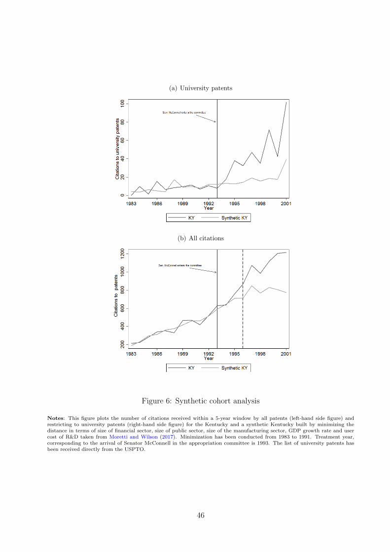
(a) University patents

(b) All citations

Figure 6: Synthetic cohort analysis

Notes: This figure plots the number of citations received within a 5-year window by all patents (left-hand side figure) andrestricting to university patents (right-hand side figure) for the Kentucky and a synthetic Kentucky built by minimizing thedistance in terms of size of financial sector, size of public sector, size of the manufacturing sector, GDP growth rate and usercost of R&D taken from Moretti and Wilson (2017). Minimization has been conducted from 1983 to 1991. Treatment year,corresponding to the arrival of Senator McConnell in the appropriation committee is 1993. The list of university patents hasbeen received directly from the USPTO.

46

(a) Earmarks (b) Citations to university patents

(c) Citations to all patents

Figure 7: Event studies

Notes: This figure plots the average share of earmarks, citations to university patents and all citations at different timesaround the appointment of a senator in the appropriation committee. All measures have been residualized on a state-specifictime trend. Sample is restricted to years 1991-2008 for the top-left panel, 1980-2006 for the top-right panel and 1976-2006 forthe bottom panel, and to states which experienced one, and only one, positive change in their representation on the committee.The vertical solid line corresponds to the arrival of a new senator in the committee, the dashed line corresponds to 3 years afterthis event. The list of university patents has been received directly from the USPTO. The list of earmarks has been receivedfrom Cohen et al. (2011).

47

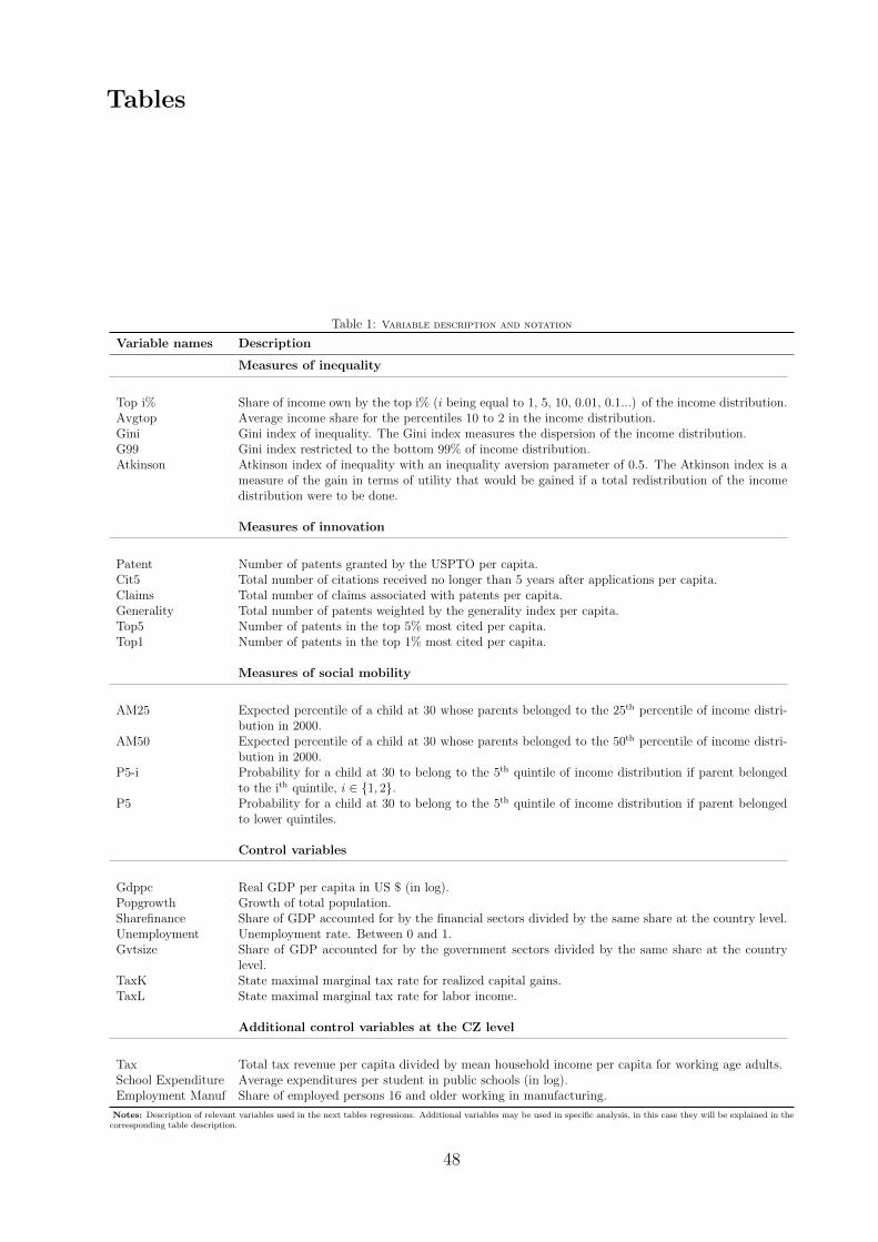
Tables

Table 1: Variable description and notation

Variable names Description

Measures of inequality

Top i% Share of income own by the top i% (i being equal to 1, 5, 10, 0.01, 0.1...) of the income distribution.Avgtop Average income share for the percentiles 10 to 2 in the income distribution.Gini Gini index of inequality. The Gini index measures the dispersion of the income distribution.G99 Gini index restricted to the bottom 99% of income distribution.Atkinson Atkinson index of inequality with an inequality aversion parameter of 0.5. The Atkinson index is a

measure of the gain in terms of utility that would be gained if a total redistribution of the incomedistribution were to be done.

Measures of innovation

Patent Number of patents granted by the USPTO per capita.Cit5 Total number of citations received no longer than 5 years after applications per capita.Claims Total number of claims associated with patents per capita.Generality Total number of patents weighted by the generality index per capita.Top5 Number of patents in the top 5% most cited per capita.Top1 Number of patents in the top 1% most cited per capita.

Measures of social mobility

AM25 Expected percentile of a child at 30 whose parents belonged to the 25th percentile of income distri-bution in 2000.

AM50 Expected percentile of a child at 30 whose parents belonged to the 50th percentile of income distri-bution in 2000.

P5-i Probability for a child at 30 to belong to the 5th quintile of income distribution if parent belongedto the ith quintile, i ∈ {1, 2}.

P5 Probability for a child at 30 to belong to the 5th quintile of income distribution if parent belongedto lower quintiles.

Control variables

Gdppc Real GDP per capita in US $ (in log).Popgrowth Growth of total population.Sharefinance Share of GDP accounted for by the financial sectors divided by the same share at the country level.Unemployment Unemployment rate. Between 0 and 1.Gvtsize Share of GDP accounted for by the government sectors divided by the same share at the country

level.TaxK State maximal marginal tax rate for realized capital gains.TaxL State maximal marginal tax rate for labor income.

Additional control variables at the CZ level

Tax Total tax revenue per capita divided by mean household income per capita for working age adults.School Expenditure Average expenditures per student in public schools (in log).Employment Manuf Share of employed persons 16 and older working in manufacturing.

Notes: Description of relevant variables used in the next tables regressions. Additional variables may be used in specific analysis, in this case they will be explained in thecorresponding table description.

48

Table 2: Descriptive statistics by measures of innovationand for the top 1% income share in two distinctive years

1980 Mean p25 p50 p75 Min Max

Top 1% 9.45 8.37 9.31 10.09 5.33 14.48Patents 140 71 113 186 27 501Cit5 146 64 113 209 21 588Claims 1,347 659 1,041 2,004 222 5,390Generality 27 12 20 36 3 130Top5 8 3 5 12 0 41Top1 3 1 2 4 0 13

2005 Mean p25 p50 p75 Min Max

Top 1% 19.07 16.12 17.65 20.77 12.47 33.3Patents 296 131 230 403 47 904Cit5 508 161 373 618 44 1,689Claims 4,567 1,915 3,045 5,599 630 24,964Generality 104 50 82 152 19 366Top5 10 2 7 12 0 36Top1 2 1 1 3 0 9

Notes: Summary statistics includes mean, quartiles’ thresholds, minimum andmaximum for our six measures of innovation and the top 1% income share (relevantvariables are defined in Table 1). All innovation measures are taken per million ofinhabitants.

Table 3: Mean and Standard Deviation ofthe main variables

Mean Std dev

Top 1% (log) 2.591 0.267Patent (log) 5.105 0.764Cit5 (log) 5.678 1.074Gdppc (log) 10.49 0.319Popgrowth 0.010 0.011Finance 0.920 0.237Government 1.033 0.273Unemployment 5.940 2.051TaxK 4.386 2.948TaxL 5.297 3.267

Notes: Mean value and standard deviation for the mainvariables calculated over the period 1980-2005 (relevantvariables are defined in Table 1). GDP per capita is calcu-lated in $ per capita and the innovation measures are takenper million of inhabitants.

49

Table 4: Top 1% income share and innovation

Dependent variable Log of Top 1% Income Share

(1) (2) (3) (4) (5) (6)Measure of innovation Patents Cit5 Claims Generality Top5 Top1

Innovation 0.031*** 0.049*** 0.017* 0.024** 0.026*** 0.020***(0.011) (0.009) (0.009) (0.010) (0.005) (0.004)

Gdppc 0.089** 0.063 0.096** 0.093** 0.074* 0.087**(0.043) (0.044) (0.045) (0.043) (0.043) (0.043)

Popgrowth 0.943 1.089 0.943 0.934 0.990 1.074(0.654) (0.700) (0.651) (0.647) (0.690) (0.685)

Finance 0.080** 0.109*** 0.072** 0.078** 0.098*** 0.094***(0.035) (0.036) (0.035) (0.035) (0.035) (0.035)

Government -0.018 -0.019* -0.018 -0.018 -0.018 -0.016(0.011) (0.011) (0.011) (0.011) (0.011) (0.011)

Unemployment -0.006** -0.006* -0.005* -0.006* -0.006* -0.005(0.003) (0.003) (0.003) (0.003) (0.003) (0.003)

TaxK -0.038*** -0.039*** -0.038*** -0.038*** -0.038*** -0.037***(0.004) (0.004) (0.004) (0.004) (0.004) (0.004)

TaxL 0.017*** 0.014** 0.017*** 0.018*** 0.013** 0.013**(0.006) (0.006) (0.006) (0.006) (0.006) (0.006)

R2 0.889 0.896 0.889 0.889 0.895 0.895Observations 1734 1581 1734 1734 1581 1581

Notes: Variable description is given in Table 1. Innovation is taken in log and lagged by two years. The dependent variable is thelog of the top 1% income share. Panel data OLS regressions with state and year fixed effects. Time span for innovation: 1976-2009(columns 1, 3 and 4) and 1976-2006 (columns 2, 5 and 6). Autocorrelation and heteroskedasticity robust standard errors usingthe Newey-West variance estimator are presented in parentheses. ***, ** and * respectively indicate 0.01, 0.05 and 0.1 levels ofsignificance.

50

Table 5: Innovation and various measures of inequality

Dependent variable Top 1% Top 10 % Avgtop Overall Gini G99 Atkinson

(1) (2) (3) (4) (5) (6)Measure of innovation Cit5 Cit5 Cit5 Cit5 Cit5 Cit5

Innovation 0.049*** 0.022*** 0.007 -0.001 -0.010** 0.017***(0.009) (0.006) (0.005) (0.003) (0.005) (0.004)

Gdppc 0.063 0.032 0.002 0.004 -0.021 0.131***(0.044) (0.028) (0.030) (0.024) (0.028) (0.029)

Popgrowth 1.089 0.553 0.265 -0.382** -0.553** 0.402(0.700) (0.424) (0.381) (0.184) (0.240) (0.276)

Finance 0.109*** 0.066*** 0.021 0.011 -0.018 0.037**(0.036) (0.020) (0.017) (0.012) (0.015) (0.018)

Government -0.019* -0.005 0.013* -0.004 0.001 -0.029***(0.011) (0.007) (0.007) (0.004) (0.005) (0.006)

Unemployment -0.006* -0.001 0.002 -0.000 0.002 -0.001(0.003) (0.002) (0.002) (0.001) (0.002) (0.001)

TaxK -0.039*** -0.018*** -0.002 -0.007*** -0.001 -0.018***(0.004) (0.003) (0.002) (0.001) (0.002) (0.002)

TaxL 0.014** 0.007* -0.001 0.004** 0.001 0.011***(0.006) (0.004) (0.003) (0.002) (0.003) (0.003)

R2 0.896 0.818 0.420 0.865 0.730 0.942Observations 1581 1581 1581 1581 1581 1581

Notes: Variable description is given in Table 1. Innovation is taken in log and lagged by two years. Panel data OLS regressionswith state and year fixed effects. Time span for innovation: 1976-2006. Autocorrelation and heteroskedasticity robust standarderrors using the Newey-West variance estimator are presented in parentheses. ***, ** and * respectively indicate 0.01, 0.05 and 0.1levels of significance.

51

Table 6: Innovation and various measures of inequality based on different income shares

Dependent variable Top 10% Top 5% Top 1% Top 0.5% Top 0.1% Top 0.01%

(1) (2) (3) (4) (5) (6)Measure of innovation Cit5 Cit5 Cit5 Cit5 Cit5 Cit5

Innovation 0.022*** 0.026*** 0.049*** 0.060*** 0.076*** 0.094***(0.006) (0.006) (0.009) (0.010) (0.013) (0.019)

Gdppc 0.032 0.050 0.063 0.055 0.060 0.046(0.028) (0.036) (0.044) (0.055) (0.068) (0.095)

Popgrowth 0.553 0.618 1.089 1.595* 2.289** 3.307**(0.424) (0.466) (0.700) (0.829) (1.120) (1.567)

Finance 0.066*** 0.063** 0.109*** 0.124*** 0.079 0.021(0.020) (0.025) (0.036) (0.046) (0.072) (0.106)

Government -0.005 -0.009 -0.019* -0.020* -0.014 0.014(0.007) (0.008) (0.011) (0.011) (0.013) (0.018)

Unemployment -0.001 -0.005** -0.006* -0.008** -0.010* -0.014**(0.002) (0.002) (0.003) (0.004) (0.005) (0.007)

TaxK -0.018*** -0.023*** -0.039*** -0.047*** -0.061*** -0.084***(0.003) (0.003) (0.004) (0.005) (0.006) (0.009)

TaxL 0.007* 0.012*** 0.014** 0.018*** 0.024*** 0.031**(0.004) (0.004) (0.006) (0.007) (0.009) (0.012)

R2 0.818 0.877 0.896 0.893 0.891 0.864Observations 1581 1581 1581 1581 1581 1581

Notes: Variable description is given in Table 1. Innovation is taken in log and lagged by two years. The dependent variables aretaken in log. Panel data OLS regressions with state and year fixed effects. Time span for innovation: 1976-2006. Autocorrelationand heteroskedasticity robust standard errors using the Newey-West variance estimator are presented in parentheses. ***, ** and *respectively indicate 0.01, 0.05 and 0.1 levels of significance.

52

Table 7: Top 1% income share and innovation by entrants and incumbents

Dependent variable Log of Top 1% Income Share

(1) (2) (3) (4) (5) (6)

Measure of innovation Patents Patents Patents Cit5 Cit5 Cit5

Innovationby entrants 0.015* 0.011 0.017*** 0.014**

(0.008) (0.008) (0.006) (0.006)by incumbents 0.018*** 0.016** 0.025*** 0.022***

(0.007) (0.007) (0.006) (0.006)Gdppc 0.110** 0.082 0.093* 0.080 0.054 0.056

(0.052) (0.055) (0.053) (0.059) (0.060) (0.058)popgrowth 2.044*** 1.997*** 2.106*** 2.287*** 2.133*** 2.208***

(0.748) (0.749) (0.755) (0.833) (0.816) (0.832)Finance 0.097*** 0.112*** 0.107*** 0.110*** 0.135*** 0.131***

(0.032) (0.032) (0.032) (0.033) (0.033) (0.033)Government -0.021 -0.024 -0.019 -0.023 -0.027 -0.020

(0.021) (0.021) (0.021) (0.020) (0.021) (0.021)Unemployment -0.002 -0.003 -0.003 -0.001 -0.003 -0.003

(0.003) (0.003) (0.003) (0.004) (0.004) (0.004)TaxK -0.038*** -0.038*** -0.038*** -0.038*** -0.039*** -0.039***

(0.005) (0.005) (0.004) (0.005) (0.005) (0.005)TaxL 0.025*** 0.026*** 0.027*** 0.022*** 0.023*** 0.024***

(0.006) (0.006) (0.006) (0.007) (0.007) (0.007)

R2 0.852 0.851 0.852 0.859 0.860 0.862Observations 1530 1530 1530 1377 1377 1377

Notes: Variable description is given in Table 1. Innovation by entrants is a count of innovation that restricts to patents whoseassignee first patented less than 3 years ago. Other patents enter in the count of Innovation by incumbents. Both these measuresof innovation are taken in log and lagged by two years. Panel data OLS regressions with state and year fixed effects. Time span forinnovation: 1980-2009 (columns 1 to 3) and 1980-2006 (columns 4 to 6). Autocorrelation and heteroskedasticity robust standarderrors using the Newey-West variance estimator are presented in parentheses. ***, ** and * respectively indicate 0.01, 0.05 and 0.1levels of significance.

53

Table 8: Top 1% income share, innovation and the role of lobbying intensity

Dependent variable Log of Top 1% Income Share

(1) (2) (3) (4) (5) (6)Measure of innovation Patents Cit5 Claims Patents Cit5 Claims

Innovationby entrants 0.905*** 0.527** 0.837***

(0.000) (0.014) (0.000)by incumbents 0.246 0.196 0.307*

(0.172) (0.312) (0.091)Lobbying×Innovation

by entrants -0.051*** -0.030** -0.048***(0.000) (0.015) (0.000)

by incumbents -0.016 -0.011 -0.019*(0.132) (0.320) (0.073)

Lobbying -0.305 -0.151 -0.095 0.053 -0.100 0.079(0.245) (0.468) (0.683) (0.813) (0.631) (0.707)

Gdppc 0.107 0.014 0.105 0.095 -0.013 0.091(0.384) (0.924) (0.397) (0.473) (0.929) (0.482)

Popgrowth 0.401 -0.146 0.379 0.640 0.150 0.622(0.738) (0.897) (0.754) (0.613) (0.902) (0.622)

Finance -0.021 -0.062 -0.027 -0.019 -0.057 -0.018(0.726) (0.326) (0.663) (0.749) (0.348) (0.754)

Government -0.107* -0.189*** -0.108* -0.117* -0.221*** -0.115*(0.085) (0.006) (0.086) (0.066) (0.001) (0.064)

Unemployment -0.010** -0.022*** -0.010** -0.011** -0.023*** -0.011**(0.026) (0.000) (0.023) (0.016) (0.000) (0.015)

TaxK -0.013** -0.014** -0.012** -0.013** -0.015*** -0.013**(0.025) (0.012) (0.028) (0.023) (0.010) (0.022)

TaxL -0.002 0.003 -0.003 -0.002 0.003 -0.002(0.840) (0.815) (0.815) (0.844) (0.811) (0.884)

R2 0.684 0.739 0.685 0.678 0.734 0.677Observations 714 561 714 714 561 714

Notes: Lobbying is measured as explained in subsection 4.4. Other variable description is given in Table 1. Innovation is taken inlog and lagged by two years. Columns 1 to 3 consider entrant innovation whether columns 4 to 6 consider incumbent innovations.The dependent variable is taken in log. Panel data OLS regressions with state and year fixed effects. Time span for innovation:1996-2009 (columns 1, 3, 4 and 6) and 1996-2005 (columns 2 and 5). Autocorrelation and heteroskedasticity robust standard errorsusing the Newey-West variance estimator are presented in parentheses. ***, ** and * respectively indicate 0.01, 0.05 and 0.1 levelsof significance.

54

Table 9: Top 1% income share and innovation at different lags

Dependent variable Log of Top 1% Income Share

(1) (2) (3) (4) (5) (6)Measure of innovation Cit5 Cit5 Cit5 Cit5 Cit5 Cit5Lag of innovation 2 years 3 years 4 years 5 years 6 years All lags

Innovation at t− 2 0.044*** 0.029*(0.010) (0.017)

Innovation at t− 3 0.040*** 0.016(0.009) (0.015)

Innovation at t− 4 0.039*** 0.022(0.009) (0.016)

Innovation at t− 5 0.030*** -0.003(0.009) (0.014)

Innovation at t− 6 0.022** -0.019(0.010) (0.016)

Gdppc 0.034 0.035 0.033 0.045 0.057 0.027(0.062) (0.062) (0.062) (0.062) (0.061) (0.063)

Popgrowth 2.210*** 2.267*** 2.307*** 2.281*** 2.296*** 2.204***(0.839) (0.838) (0.827) (0.829) (0.828) (0.846)

Finance 0.139*** 0.134*** 0.133*** 0.126*** 0.121*** 0.141***(0.034) (0.033) (0.033) (0.033) (0.034) (0.035)

Government -0.025 -0.027 -0.028 -0.029 -0.030 -0.024(0.019) (0.019) (0.019) (0.020) (0.020) (0.019)

Unemployment -0.003 -0.003 -0.003 -0.002 -0.002 -0.004(0.004) (0.004) (0.004) (0.004) (0.004) (0.004)

TaxK -0.039*** -0.039*** -0.038*** -0.039*** -0.038*** -0.039***(0.005) (0.005) (0.005) (0.005) (0.005) (0.005)

TaxL 0.022*** 0.022*** 0.022*** 0.022*** 0.021*** 0.022***(0.007) (0.007) (0.007) (0.007) (0.007) (0.007)

R2 0.860 0.860 0.860 0.859 0.858 0.861Observations 1377 1377 1377 1377 1377 1377

Notes: Variable description is given in Table 1. Innovation is taken in log. The lag between the dependent variable and theinnovation measures ranges from 2 years to 6 years. Panel data OLS regressions with state and year fixed effects. Time span forinnovation: 1980-2006. Autocorrelation and heteroskedasticity robust standard errors using the Newey-West variance estimator arepresented in parentheses. ***, ** and * respectively indicate 0.01, 0.05 and 0.1 levels of significance.

55

Table 10: Senate Appropriation Committee composition and earmarks

Dependent variable Log of earmarks Cit5 univ

All earmarks Research earmarks

(1) (2) (3) (4) (5) (6)

SenateMember 0.401*** 0.331*** 0.330*** 0.310*** 0.096** 0.089**(0.076) (0.074) (0.113) (0.103) (0.048) (0.037)

Gdppc -1.003 -0.327 -4.092*** -3.182*** 0.746** 0.448(0.708) (0.703) (1.002) (0.988) (0.367) (0.283)

Ppgrowth -0.805 -2.825 2.623 1.949 -4.337 -2.851(5.519) (5.111) (8.062) (7.659) (3.411) (2.726)

Finance 0.651 0.213 0.292 0.290 -1.018*** -0.606***(0.479) (0.422) (0.601) (0.524) (0.253) (0.203)

Government -0.144 0.228 0.333 0.059 0.169 0.134(0.518) (0.522) (0.532) (0.559) (0.103) (0.095)

Unemployment -0.016 -0.016 -0.101* -0.050 -0.052** -0.030(0.037) (0.031) (0.055) (0.054) (0.022) (0.018)

TaxK 0.050 0.085* 0.052 0.038 -0.025 -0.013(0.047) (0.047) (0.062) (0.056) (0.030) (0.024)

TaxL -0.062 -0.174* -0.287** -0.127 0.133*** 0.083**(0.089) (0.101) (0.142) (0.131) (0.046) (0.036)

Yi,t−1 0.160*** 0.201*** 0.338***(0.039) (0.040) (0.031)

R2 0.636 0.637 0.426 0.449 0.588 0.637Observations 918 867 918 867 1428 1428

Notes: The dependent variable in columns 1 to 4 is the log of total earmarks received per capita in the state and comesfrom Cohen et al. (2011). Research earmarks have been selected based on the title on the appropriation bill. Columns 5and 6 used the citations received within a 5-year window to patent assigned to universities. Panel data OLS regressions withstate and year fixed effects. Yi,t−1 denotes the lagged value of the dependent variable. Other variables description is given inTable 1. Autocorrelation and heteroskedasticity robust standard errors computed using the Newey-West variance estimatorare reported in parentheses. ***, ** and * respectively indicate 0.01, 0.05 and 0.1 levels of significance.

56

Table 11: Regression of innovation on top 1% income share using instrument based on Appro-priation Committee composition in the Senate

Dependent variable Log of Top 1% Income Share

(1) (2) (3) (4) (5) (6)Measure of innovation Patents Cit5 Claims Generality Top5 Top1

Innovation 0.220** 0.185** 0.201** 0.233** 0.143** 0.153**(0.102) (0.078) (0.100) (0.113) (0.066) (0.074)

Gdppc -0.103 -0.079 -0.151 -0.138 -0.104 -0.079(0.109) (0.093) (0.138) (0.130) (0.107) (0.102)

popgrowth 1.960** 1.663* 2.348** 2.101** 1.534* 1.886**(0.937) (0.969) (1.034) (0.949) (0.932) (0.961)

Finance 0.179*** 0.213*** 0.175*** 0.198*** 0.209*** 0.232***(0.061) (0.068) (0.066) (0.073) (0.073) (0.086)

Government -0.097*** -0.078*** -0.099*** -0.101*** -0.037 -0.014(0.024) (0.024) (0.025) (0.027) (0.030) (0.042)

Unemployment -0.012** -0.012** -0.013** -0.014** -0.012** -0.007(0.005) (0.005) (0.006) (0.006) (0.005) (0.005)

TaxK -0.040*** -0.039*** -0.041*** -0.043*** -0.039*** -0.036***(0.005) (0.005) (0.006) (0.006) (0.005) (0.005)

TaxL 0.022*** 0.016** 0.025*** 0.027*** 0.014** 0.014*(0.008) (0.007) (0.009) (0.010) (0.007) (0.008)

Highways 0.398 0.511 0.454 0.427 0.417 0.669(0.448) (0.464) (0.486) (0.489) (0.452) (0.541)

Military -0.002 -0.004 -0.003 -0.002 -0.008 -0.004(0.007) (0.008) (0.008) (0.009) (0.008) (0.008)

R2 0.866 0.874 0.851 0.846 0.844 0.812F-stat on the excludedinstruments

15.5 14.2 12.2 10.4 10.7 7.6

Observations 1700 1550 1700 1700 1550 1550

Notes: Variable description is given in Table 1. Innovation is taken in log and lagged by two years. Panel data IV 2SLS regressionswith state and year fixed effects. Innovation is instrumented by the number of senators that sit on the appropriation committee.The lag between the instrument and the endogenous variable is set to 3 years. Time span for innovation: 1976-2009 for columns1, 3 and 4 and 1976-2006 for columns 2, 5 and 6. DC is removed from the sample because it has no senators. Autocorrelationand heteroskedasticity robust standard errors using the Newey-West variance estimator are presented in parentheses. ***, ** and *respectively indicate 0.01, 0.05 and 0.1 levels of significance.

57

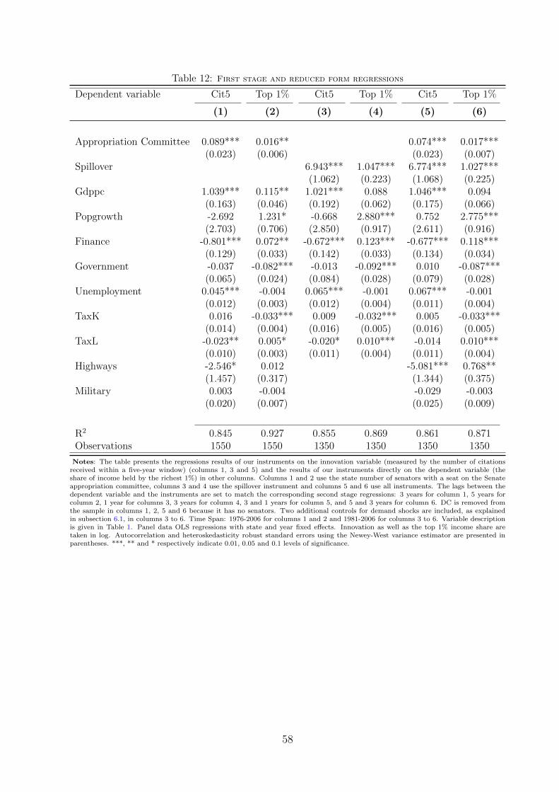
Table 12: First stage and reduced form regressions

Dependent variable Cit5 Top 1% Cit5 Top 1% Cit5 Top 1%

(1) (2) (3) (4) (5) (6)

Appropriation Committee 0.089*** 0.016** 0.074*** 0.017***(0.023) (0.006) (0.023) (0.007)

Spillover 6.943*** 1.047*** 6.774*** 1.027***(1.062) (0.223) (1.068) (0.225)

Gdppc 1.039*** 0.115** 1.021*** 0.088 1.046*** 0.094(0.163) (0.046) (0.192) (0.062) (0.175) (0.066)

Popgrowth -2.692 1.231* -0.668 2.880*** 0.752 2.775***(2.703) (0.706) (2.850) (0.917) (2.611) (0.916)

Finance -0.801*** 0.072** -0.672*** 0.123*** -0.677*** 0.118***(0.129) (0.033) (0.142) (0.033) (0.134) (0.034)

Government -0.037 -0.082*** -0.013 -0.092*** 0.010 -0.087***(0.065) (0.024) (0.084) (0.028) (0.079) (0.028)

Unemployment 0.045*** -0.004 0.065*** -0.001 0.067*** -0.001(0.012) (0.003) (0.012) (0.004) (0.011) (0.004)

TaxK 0.016 -0.033*** 0.009 -0.032*** 0.005 -0.033***(0.014) (0.004) (0.016) (0.005) (0.016) (0.005)

TaxL -0.023** 0.005* -0.020* 0.010*** -0.014 0.010***(0.010) (0.003) (0.011) (0.004) (0.011) (0.004)

Highways -2.546* 0.012 -5.081*** 0.768**(1.457) (0.317) (1.344) (0.375)

Military 0.003 -0.004 -0.029 -0.003(0.020) (0.007) (0.025) (0.009)

R2 0.845 0.927 0.855 0.869 0.861 0.871Observations 1550 1550 1350 1350 1350 1350

Notes: The table presents the regressions results of our instruments on the innovation variable (measured by the number of citationsreceived within a five-year window) (columns 1, 3 and 5) and the results of our instruments directly on the dependent variable (theshare of income held by the richest 1%) in other columns. Columns 1 and 2 use the state number of senators with a seat on the Senateappropriation committee, columns 3 and 4 use the spillover instrument and columns 5 and 6 use all instruments. The lags between thedependent variable and the instruments are set to match the corresponding second stage regressions: 3 years for column 1, 5 years forcolumn 2, 1 year for columns 3, 3 years for column 4, 3 and 1 years for column 5, and 5 and 3 years for column 6. DC is removed fromthe sample in columns 1, 2, 5 and 6 because it has no senators. Two additional controls for demand shocks are included, as explainedin subsection 6.1, in columns 3 to 6. Time Span: 1976-2006 for columns 1 and 2 and 1981-2006 for columns 3 to 6. Variable descriptionis given in Table 1. Panel data OLS regressions with state and year fixed effects. Innovation as well as the top 1% income share aretaken in log. Autocorrelation and heteroskedasticity robust standard errors using the Newey-West variance estimator are presented inparentheses. ***, ** and * respectively indicate 0.01, 0.05 and 0.1 levels of significance.

58

Table 13: Simulation results

Moments Parameters

Definition and source Target Simulations

M1Average top 1% share (own data) 0.130 0.13 ηL= 1.16M2 Ratio of entrant to incumbent citations (own data) 0.2 0.25 ηH= 1.35M3 Elasticity of top 1% w.r.t innovation (Garcia-Macia et al., 2016)

0.185 0.184 θI= 0.7

M4 Average mark-up (Jaimovich and Floetotto,2008)

1.2 1.20 θE= 7.3

M5 Entrant share of employment (own data) 0.03 0.031 L = 74.8M6 Growth rate 0.02 0.020 φ = 0.196

Notes: Definition and value of the targeted moments, average value for the targeted moments in 500 draws of simulateddata and parameters

59

Table 14: Top 1% income share and innovation - CZ level panel

Dependent variable Log of Top 1% Income Share

(1) (2) (3) (4) (5)Measure of innovation Patents Patents Patents Patents Patents

Innovation 0.021* 0.019* 0.019* 0.019* 0.018*(0.012) (0.011) (0.011) (0.011) (0.010)

Gdppc -0.352 -0.359 -0.540** -0.596**(0.217) (0.217) (0.260) (0.288)

Popgrowth 0.333 0.277 0.011(0.561) (0.508) (0.428)

Finance 0.002 0.007(0.086) (0.088)

Government -0.187** -0.166**(0.088) (0.078)

Unemployment -1.814(1.452)

R2 0.816 0.818 0.812 0.813 0.814Observations 5599 5599 5571 5570 5570

Notes: Variable description is given in Table 1. A dummy equal to one if the CZ belongs to an urbanarea is included but not reported. Panel fixed effect regression with CZs weighted by population andstate×year dummies. Time span for innovation: 1998 and 2003-2009. Regressions also include a dummyfor being an urban CZ. Heteroskedasticity robust standard errors clustered at the state level are reportedin parentheses. ***, ** and * respectively indicate 0.01, 0.05 and 0.1 levels of significance.

60

Table 15: Innovation and social mobility at the Commuting Zone level

Dependent variable AM25 P1-5 P2-5 AM25 P1-5 P2-5 P5

(1) (2) (3) (4) (5) (6) (7)Measure of innovation Cit5 Cit5 Cit5 Cit5 Cit5 Cit5 Cit5

Innovation 0.015 0.076* 0.028 0.023** 0.112** 0.053** 0.012(0.010) (0.042) (0.025) (0.010) (0.042) (0.025) (0.017)

Gdppc 0.025 0.416* 0.158 -0.074 0.007 -0.144 -0.051(0.054) (0.235) (0.136) (0.062) (0.255) (0.148) (0.106)

Popgrowth -1.156 -1.322 -5.852** -1.944** -4.976 -8.218*** -7.210***(0.850) (3.667) (2.539) (0.838) (3.628) (2.288) (1.600)

Government 0.047 0.263* 0.119 0.038 0.227 0.088 0.051(0.032) (0.133) (0.090) (0.033) (0.138) (0.093) (0.066)

Finance 0.032 0.035 0.093* 0.016 -0.023 0.045 0.046(0.021) (0.083) (0.054) (0.019) (0.073) (0.054) (0.039)

Unemployment -0.025 0.720 -0.202 -0.201 -0.026 -0.740 -0.723*(0.212) (0.908) (0.604) (0.211) (0.872) (0.550) (0.398)

Tax 0.000 0.001 0.001 -0.001 -0.004 -0.003 -0.001(0.001) (0.006) (0.004) (0.002) (0.006) (0.005) (0.004)

School Expenditure 0.008 0.027 0.024 0.016(0.009) (0.034) (0.024) (0.019)

Employment Manuf -0.391*** -1.682*** -1.177*** -0.720***(0.110) (0.401) (0.332) (0.247)

R2 0.146 0.180 0.168 0.197 0.225 0.218 0.264Observations 666 674 674 662 670 670 670

Notes: Variable description is given in Table 1. The number of citations per inhabitants is averaged over the period 1998-2008 and socialmobility measures are taken when the child is 30 between 2011 and 2012, compared to his parents during the period 1996-2000. All thesemeasures are taken in logs. Cross section OLS regressions with CZs weighted by population. Regressions also include a dummy for beingan urban CZ. Heteroskedasticity robust standard errors clustered at the state level are reported in parentheses. ***, ** and * respectivelyindicate 0.01, 0.05 and 0.1 levels of significance.

61

Table 16: Innovation and social mobility at the Commuting Zone level. Entrantsand incumbents innovation and lobbying

Dependent variable AM25

(1) (2) (3) (4) (5)Measure of innovation Cit5 Cit5 Cit5 Cit5 Cit5

Innovationby entrants 0.023** 0.019* 0.001 0.035***

(0.009) (0.009) (0.007) (0.012)by incumbents 0.016** 0.006 0.001 0.004

(0.008) (0.007) (0.006) (0.008)Gdppc -0.081 -0.047 -0.086 -0.058 -0.087

(0.057) (0.064) (0.058) (0.108) (0.054)Popgrowth -1.774** -1.847** -1.827** -3.428** -0.907

(0.821) (0.837) (0.863) (1.293) (0.968)Finance 0.018 0.017 0.018 0.032 0.015

(0.018) (0.019) (0.019) (0.025) (0.021)Government 0.035 0.039 0.035 -0.019 0.036

(0.033) (0.035) (0.033) (0.023) (0.040)Participation Rate 0.225 0.199 0.203 0.896** -0.054

(0.208) (0.217) (0.210) (0.338) (0.217)Tax -0.001 -0.001 -0.001 0.001 -0.001

(0.002) (0.002) (0.002) (0.002) (0.001)School Expenditure 0.010 0.007 0.009 0.015 0.013

(0.009) (0.009) (0.009) (0.009) (0.009)Employment Manuf -0.334*** -0.384*** -0.358*** -0.305*** -0.304**

(0.109) (0.113) (0.113) (0.110) (0.125)

R2 0.198 0.185 0.201 0.404 0.269Observations 662 662 662 328 334

Notes: Variable description is given in Table 1. The number of citations per inhabitants is averaged over theperiod 1998-2008 and social mobility measures are taken when the child is 30 between 2011 and 2012 compared tohis parents during the period 1996-2000. All these measures are taken in logs. Column 4 restricts to CZs abovemedian in terms of lobbying intensity, where lobbying is measured as explained in subsection 8.2 while column 5restricts to CZs below median. A dummy equal to one if the CZ belongs to an urban area is included but notreported. Cross section OLS regressions with CZs weighted by population. Heteroskedasticity robust standarderrors clustered at the state level are reported in parentheses. ***, ** and * respectively indicate 0.01, 0.05 and0.1 levels of significance.

62