General rights Copyright and moral rights for the publications made accessible in the public portal are retained by the authors and/or other copyright owners and it is a condition of accessing publications that users recognise and abide by the legal requirements associated with these rights.

• Users may download and print one copy of any publication from the public portal for the purpose of private study or research. • You may not further distribute the material or use it for any profit-making activity or commercial gain • You may freely distribute the URL identifying the publication in the public portal

If you believe that this document breaches copyright please contact us providing details, and we will remove access to the work immediately and investigate your claim.

Downloaded from orbit.dtu.dk on: Jun 16, 2018

Instability of vortex pair leapfrogging

Tophøj, Laust Emil Hjerrild; Aref, Hassan

Published in:Physics of Fluids

Link to article, DOI:10.1063/1.4774333

Publication date:2013

Document VersionPublisher's PDF, also known as Version of record

Link back to DTU Orbit

Citation (APA):Tophøj, L., & Aref, H. (2013). Instability of vortex pair leapfrogging. Physics of Fluids, 25(1), 014107. DOI:10.1063/1.4774333

Instability of vortex pair leapfroggingLaust Tophøj and Hassan Aref Citation: Phys. Fluids 25, 014107 (2013); doi: 10.1063/1.4774333 View online: http://dx.doi.org/10.1063/1.4774333 View Table of Contents: http://pof.aip.org/resource/1/PHFLE6/v25/i1 Published by the American Institute of Physics. Related ArticlesBistability and hysteresis of maximum-entropy states in decaying two-dimensional turbulence Phys. Fluids 25, 015113 (2013) Experimental study on side force alleviation of conical forebody with a fluttering flag Phys. Fluids 24, 124105 (2012) Effects of passive control rings positioned in the shear layer and potential core of a turbulent round jet Phys. Fluids 24, 115103 (2012) Vortex formation and instability in the left ventricle Phys. Fluids 24, 091110 (2012) Structure and stability of the finite-area von Kármán street Phys. Fluids 24, 066602 (2012) Additional information on Phys. FluidsJournal Homepage: http://pof.aip.org/ Journal Information: http://pof.aip.org/about/about_the_journal Top downloads: http://pof.aip.org/features/most_downloaded Information for Authors: http://pof.aip.org/authors

Downloaded 22 Feb 2013 to 192.38.67.112. Redistribution subject to AIP license or copyright; see http://pof.aip.org/about/rights_and_permissions

PHYSICS OF FLUIDS 25, 014107 (2013)

Instability of vortex pair leapfroggingLaust Tophøj1,2,a) and Hassan Aref2,3

1Department of Physics, Technical University of Denmark, Kongens Lyngby,DK-2800, Denmark2Center for Fluid Dynamics, Technical University of Denmark, Kongens Lyngby,DK-2800, Denmark3Department of Engineering Science and Mechanics, Virginia Tech, Blacksburg,Virginia 24061, USA

(Received 1 March 2012; accepted 28 September 2012; published online 30 January 2013)

Leapfrogging is a periodic solution of the four-vortex problem with two positiveand two negative point vortices all of the same absolute circulation arranged asco-axial vortex pairs. The set of co-axial motions can be parameterized by theratio 0 < α < 1 of vortex pair sizes at the time when one pair passes throughthe other. Leapfrogging occurs for α > σ 2, where σ = √

2 − 1 is the silver ra-tio. The motion is known in full analytical detail since the 1877 thesis of Grobliand a well known 1894 paper by Love. Acheson [“Instability of vortex leapfrog-ging,” Eur. J. Phys. 21, 269–273 (2000)] determined by numerical experimentsthat leapfrogging is linearly unstable for σ 2 < α < 0.382, but apparently sta-ble for larger α. Here we derive a linear system of equations governing smallperturbations of the leapfrogging motion. We show that symmetry-breaking per-turbations are essentially governed by a 2D linear system with time-periodic co-efficients and perform a Floquet analysis. We find transition from linearly unsta-ble to stable leapfrogging at α = φ2 ≈ 0.381966, where φ = 1

2 (√

5 − 1) is thegolden ratio. Acheson also suggested that there was a sharp transition between a“disintegration” instability mode, where two pairs fly off to infinity, and a “walk-about” mode, where the vortices depart from leapfrogging but still remain withina finite distance of one another. We show numerically that this transition is moregradual, a result that we relate to earlier investigations of chaotic scattering ofvortex pairs [L. Tophøj and H. Aref, “Chaotic scattering of two identical pointvortex pairs revisited,” Phys. Fluids 20, 093605 (2008)]. Both leapfrogging and“walkabout” motions can appear as intermediate states in chaotic scattering at thesame values of linear impulse and energy. C© 2013 American Institute of Physics.[http://dx.doi.org/10.1063/1.4774333]

I. INTRODUCTION

The possibility that two vortex rings with a common axis can “leapfrog” was already mentionedby Helmholtz in his original paper on vortex dynamics.1 He wrote (in Tait’s translation): “We cannow see generally how two ring-formed vortex-filaments having the same axis would mutually affecteach other. . . the foremost widens and travels more slowly, the pursuer shrinks and travels faster,till finally, if their velocities are not too different, it overtakes the first and penetrates it. Then thesame game goes on in the opposite order, so that the rings pass through each other alternately.” Pipesmokers skilled in blowing smoke rings will often blow two rings in succession demonstrating the

a)Electronic mail: laustemil@gmail.com.

1070-6631/2013/25(1)/014107/17/$30.00 C©2013 American Institute of Physics25, 014107-1

Downloaded 22 Feb 2013 to 192.38.67.112. Redistribution subject to AIP license or copyright; see http://pof.aip.org/about/rights_and_permissions

014107-2 L. Tophøj and H. Aref Phys. Fluids 25, 014107 (2013)

phenomenon. A more precise and often-cited flow visualization experiment was performed manyyears ago.2 A mathematical discussion of the dynamics of thin-filament vortex rings with symmetrycan be found in Ref. 3.

Here we are interested in the two-dimensional counterpart, where two co-axial vortex pairsleapfrog one another, in the special case when the four vortices all have the same absolute circu-lation. The analytical solution of this periodic motion, when the vortices are represented as pointvortices, was derived by Grobli,4 and subsequently by Love,5 more than a century ago. Grobliand Love both found that leapfrogging was possible only if the size ratio of the two pairs at themoment one slips through the other is not too large. To quote from Love’s paper:5 “. . . the mo-tion is periodic, if, at the instant when one pair passes through the other, the ratio of the breadthsof the pairs is less than 3 + 2

√2. When the ratio has this precise value the smaller pair shoots

ahead of the larger and widens, while the larger contracts, so that each is ultimately of the samebreadth . . . , and the distance between them is ultimately infinite. When the ratio in question isgreater than 3 + 2

√2, the smaller shoots ahead and widens, and the latter falls behind and con-

tracts. . . When the ratio is less than 3 + 2√

2, the motion of the two pairs is similar to the motiondescribed by Helmholtz for two rings on the same axis, and it is probable that there is for thiscase also a critical condition in which the rings, after one has passed through the other, ultimatelyseparate to an infinite distance, and attain equal diameters.” We note that 3 + 2

√2 ≈ 5.82843 and

that (3 + 2√

2)−1 = 3 − 2√

2 ≈ 0.171573. Here 3 − 2√

2 = σ 2, where σ = √2 − 1 is called the

silver ratio.In 2000 Acheson published a short paper6 in which he reported on numerical simulations where

the classical leapfrogging solution had been slightly perturbed, in essence by rotating one of thepairs so that it no longer was symmetric with respect to the centerline of the other. Acheson thenfound that the leapfrogging motion is unstable and that it breaks down through one of two differentmodes of instability. He worked in terms of the size ratio α of the smaller pair to the larger atthe moment of slip-through. The classical solutions4, 5 show that leapfrogging requires α > σ 2

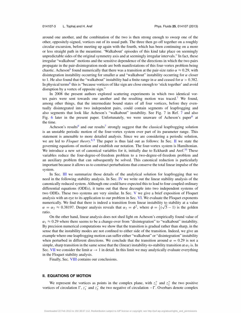
≈ 0.172. For α = 0.220, Acheson reproduced the classical solution numerically. Perturbing oneof the vortex positions by one part in 106, Acheson observed the leapfrogging to cease after a fewperiods and the four-vortex system disintegrated into two pairs that propagated off to infinity. (SeeFig. 1(a) for a similar calculation at α = 0.25.) For α = 0.310, and a larger perturbation, a differentmode of instability was observed, that Acheson termed the “walkabout” instability. Here one vortexleaves its partner, crosses the centerline, and joins with the other pair in a complicated boundedmotion while the entire system continues to move forward. This would then resolve itself back intoa leapfrogging motion. Later another “walkabout” event might take place, and so on. (See Fig. 1(b)for a similar calculation at α = 0.305.) Acheson described his observations in these words: “Whatappears to happen is that two like-signed vortices occasionally get so close that they revolve rapidly

(b)

(a)

FIG. 1. Instability calculations of leapfrogging similar to those reported by Acheson.6 Two different perturbations areshown. Vertical lines indicate the initial positions. (a) A “disintegration” instability for α = 0.25 perturbed by ξ−= η+ = −10−6. (b) A “walkabout” instability for α = 0.30 perturbed by ξ− = 0, η+ = 10−5 (see text for precisedefinitions).

Downloaded 22 Feb 2013 to 192.38.67.112. Redistribution subject to AIP license or copyright; see http://pof.aip.org/about/rights_and_permissions

014107-3 L. Tophøj and H. Aref Phys. Fluids 25, 014107 (2013)

around one another, and the combination of the two is then strong enough to sweep one of theother, oppositely-signed, vortices out of its usual path. The three then go off together on a roughlycircular excursion, before meeting up again with the fourth, which has been continuing on a moreor less straight path in the meantime. ‘Walkabout’ episodes of this kind take place on seeminglyunpredictable sides of the original symmetry axis and at seemingly irregular intervals.” In fact, theseirregular “walkabout” motions and the sensitive dependence of the directions in which the two pairspropagate in the pair-disintegration mode are both manifestations of this four-vortex problem beingchaotic. Acheson6 found numerically that there was a transition at the pair-size ratio α ≈ 0.29, withdisintegration instability occurring for smaller α and “walkabout” instability occurring for α closerto 1. He also found that the “walkabout” instability had a finite range in α and ceased for α > 0.382.In physical terms6 this is “because vortices of like sign are close enough to ‘stick together’ and avoiddisruption by a vortex of opposite sign.”

In 2008 the present authors explored scattering experiments in which two identical vor-tex pairs were sent towards one another and the resulting motion was traced.7 We found,among other things, that the intermediate bound states of all four vortices, before they even-tually disintegrated into two independent pairs, could contain segments of leapfrogging andalso segments that look like Acheson’s “walkabout” instability. See Fig. 7 in Ref. 7 and alsoFig. 6 later in the present paper. Unfortunately, we were unaware of Acheson’s paper6 atthe time.

Acheson’s results6 and our results7 strongly suggest that the classical leapfrogging solutionis an unstable periodic motion of the four-vortex system over part of its parameter range. Thisstatement is amenable to more detailed analysis. Since we are considering a periodic solution,we are led to Floquet theory.8, 9 The paper is thus laid out as follows: In Sec. II we state thegoverning equations of motion and establish our notation. The four-vortex system is Hamiltonian.We introduce a new set of canonical variables for it, initially due to Eckhardt and Aref.10 Thesevariables reduce the four-degree-of-freedom problem to a two-degree-of-freedom problem andan auxiliary problem that can subsequently be solved. This canonical reduction is particularlyimportant because it allows us to construct perturbations that conserve the total linear impulse of thesystem.

In Sec. III we summarize those details of the analytical solution for leapfrogging that weneed in the following stability analysis. In Sec. IV we write out the linear stability analysis of thecanonically reduced system. Although one could have expected this to lead to four coupled ordinarydifferential equations (ODEs), it turns out that these decouple into two independent systems oftwo ODEs. These two systems are very similar. In Sec. V we give a brief exposition of Floquetanalysis with an eye to its application to our problem in Sec. VI. We evaluate the Floquet exponentsnumerically. We find that there is indeed a transition from linear instability to stability at a valueα = α2 ≈ 0.38197. Deeper analysis reveals that α2 = φ2, where φ = 1

2 (√

5 − 1) is the goldenratio.

On the other hand, linear analysis does not shed light on Acheson’s empirically found value ofα1 ≈ 0.29 where there seems to be a change-over from “disintegration” to “walkabout” instability.By precision numerical computations we show that the transition is gradual rather than sharp, in thesense that the instability modes are not confined to either side of the transition. Indeed, we give anexample where one leapfrogging motion can suffer either “walkabout” or “disintegration” instabilitywhen perturbed in different directions. We conclude that the transition around α = 0.29 is not asimple, sharp transition in the same sense that the (linear) instability-to-stability transition at α2 is. InSec. VII we consider the limit α → 1 in detail. In this limit we may analytically evaluate everythingin the Floquet stability analysis.

Finally, Sec. VIII contains our conclusions.

II. EQUATIONS OF MOTION

We represent the vortices as points in the complex plane, with z+1 and z+

2 the two positivevortices of circulation �, z−

1 and z−2 the two negative of circulation −�. Overbars denote complex

Downloaded 22 Feb 2013 to 192.38.67.112. Redistribution subject to AIP license or copyright; see http://pof.aip.org/about/rights_and_permissions

014107-4 L. Tophøj and H. Aref Phys. Fluids 25, 014107 (2013)

conjugation. The equations of motion of our point vortex system are

dz+1

dt= �

2π i

( 1

z+1 − z+

2

− 1

z+1 − z−

1

− 1

z+1 − z−

2

),

dz+2

dt= �

2π i

( 1

z+2 − z+

1

− 1

z+2 − z−

1

− 1

z+2 − z−

2

),

dz−1

dt= �

2π i

( 1

z−1 − z+

1

+ 1

z−1 − z+

2

− 1

z−1 − z−

2

),

dz−2

dt= �

2π i

( 1

z−2 − z+

1

+ 1

z−2 − z+

2

− 1

z−2 − z−

1

),

(1)

As with all point vortex problems this system is Hamiltonian.We change to another set of variables by a canonical transformation due to Eckhardt and Aref:10

ζ0 = 12�(z+

1 + z+2 − z−

1 − z−2 ),

ζ0 = 12 (z+

1 + z+2 + z−

1 + z−2 ),

ζ+ = 12 (z+

1 − z+2 + z−

1 − z−2 ),

ζ− = 12�(z+

1 − z+2 − z−

1 + z−2 ).

(2a)

It is also useful to have the inverse transformation,

z+1 = 1

2 [ζ0 + ζ+ + (ζ0 + ζ−)/�],

z−1 = 1

2 [ζ0 + ζ+ − (ζ0 + ζ−)/�],

z+2 = 1

2 [ζ0 − ζ+ + (ζ0 − ζ−)/�],

z−2 = 1

2 [ζ0 − ζ+ − (ζ0 − ζ−)/�].

(2b)

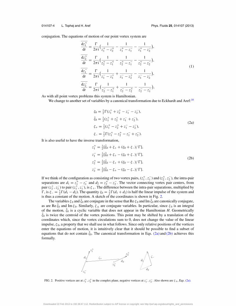
If we think of the configuration as consisting of two vortex pairs, (z+1 , z−

1 ) and (z+2 , z−

2 ), the intra-pairseparations are d1 = z+

1 − z−1 and d2 = z+

2 − z−2 . The vector connecting vortex pair centers, from

pair (z+2 , z−

2 ) to pair (z+1 , z−

1 ), is ζ+. The difference between the intra-pair separations, multiplied by�, is ζ− = 1

2�(d1 − d2). The quantity ζ0 = 12�(d1 + d2) is half the linear impulse of the system and

is thus a constant of the motion. A sketch of the coordinates is shown in Fig. 2.The variables ζ 0 and ζ0 are conjugate in the sense that Re ζ 0 and Im ζ0 are canonically conjugate,

as are Re ζ0 and Im ζ 0. Similarly, ζ± are conjugate variables. In particular, since ζ 0 is an integralof the motion, ζ0 is a cyclic variable that does not appear in the Hamiltonian H. Geometricallyζ0 is twice the centroid of the vortex positions. This point may be shifted by a translation of thecoordinates which, since the vortex circulations sum to 0, does not change the value of the linearimpulse, ζ 0, a property that we shall use in what follows. Since only relative positions of the vorticesenter the equations of motion, it is intuitively clear that it should be possible to find a subset ofequations that do not contain ζ0. The canonical transformation in Eqs. (2a) and (2b) achieves thisformally.

d1d1d2

d2

z+1

z−1

z+2

z−2

ζ+ζ−

FIG. 2. Positive vortices are at z+1 , z+

2 in the complex plane, negative vortices at z−1 , z−

2 . Also shown are ζ±, Eqs. (2a).

Downloaded 22 Feb 2013 to 192.38.67.112. Redistribution subject to AIP license or copyright; see http://pof.aip.org/about/rights_and_permissions

014107-5 L. Tophøj and H. Aref Phys. Fluids 25, 014107 (2013)

Note that a configuration that has the real axis as a symmetry axis, such as the leapfroggingmotions, i.e., for which z−

1 = z+1 , z−

2 = z+2 , must have ζ+ real and ζ− imaginary. Also note that if

we had paired up the vortices as (z+2 , z−

1 ) and (z+1 , z−

2 ), we would, in essence, have interchanged thedefinitions of ζ± (except for a factor of �). Hence, the equations of motion written in terms of ζ±must display this symmetry.

The canonical transformation implies that the equations for ζ+ and ζ− form a closed two-degree-of-freedom dynamical system, in which the constant ζ 0 enters as a parameter. According toEq. (3.14) of Ref. 10, the Hamiltonian of this reduced system is

H = − �2

2πlog

∣∣∣∣ 1

ζ 20 − ζ 2+

− 1

ζ 20 − ζ 2−

∣∣∣∣. (3)

The resulting equations of motion are

dζ+dt

= �2

iπζ−

(1

ζ 2− − ζ 2++ 1

ζ 20 − ζ 2−

),

dζ−dt

= �2

iπζ+

(1

ζ 2+ − ζ 2−+ 1

ζ 20 − ζ 2+

)

and also,

dζ0

dt= �2

iπζ0

(1

ζ 2+ − ζ 20

+ 1

ζ 2− − ζ 20

).

The case ζ 0 = 0 is integrable10 but not of particular interest for the present considerations.Assuming ζ 0 �= 0, we scale ζ± and ζ0 by −iζ 0, but again call the scaled variables ζ± and ζ0. Thisscaling guarantees that if the vortices initially are placed on the y-axis, so that the leapfrogging motionwould propagate along the x-axis, then ζ± and ζ0 are proportional to their scaled counterparts with areal coefficient of proportionality. We now obtain a common pre-factor �2/π |ζ 0|2 on the right-handsides of the preceding equations of motion. We may choose units of length and time such that thiscommon pre-factor is 1. The re-scaled equations of motion are then simply

dζ+dt

= iζ−

(1

ζ 2+ − ζ 2−+ 1

1 + ζ 2−

), (4a)

dζ−dt

= iζ+

(1

ζ 2− − ζ 2++ 1

1 + ζ 2+

), (4b)

dζ0

dt= 1

1 + ζ 2++ 1

1 + ζ 2−. (4c)

These may be derived from the re-scaled Hamiltonian, cf. (3),

H = − 12 log

∣∣∣∣ 1

1 + ζ 2+− 1

1 + ζ 2−

∣∣∣∣. (5)

The simplest way to verify that (4a) and (4b) are indeed in canonical form with H as the Hamiltonianis to consider the analytic continuation of H, viz.,

H = − 12 log

(1

1 + ζ 2+− 1

1 + ζ 2−

). (6a)

It is then easy to see that Eqs. (4a) and (4b) are simply

dζ+dt

= i∂H∂ζ−

,dζ−dt

= i∂H∂ζ+

. (6b)

Downloaded 22 Feb 2013 to 192.38.67.112. Redistribution subject to AIP license or copyright; see http://pof.aip.org/about/rights_and_permissions

014107-6 L. Tophøj and H. Aref Phys. Fluids 25, 014107 (2013)

Using the analyticity of H, and that H = ReH, we arrive at the standard Hamiltonian formulationof Eqs. (4a) and (4b).

III. LEAPFROGGING SOLUTIONS

We consider leapfrogging motions along the real axis, where the vortices are originally alignedon the y-axis. For such motions ζ 0 is imaginary and, according to (2a), ζ+ is real and ζ− imaginaryboth before and after rescaling. In Eqs. (4a) and (4b) we set

ζ+(t) = X (t), ζ−(t) = iY (t), (7a)

with X(t) and Y(t) real. In terms of these quantities Eqs. (4a) and (4b) become

dX

dt= − Y (1 + X2)

(X2 + Y 2)(1 − Y 2),

dY

dt= X (1 − Y 2)

(X2 + Y 2)(1 + X2).

(7b)

The vortices in both pairs have the real axis as a common axis of symmetry. This discrete symmetry(to flipping about the real axis and reversing the circulations) is preserved throughout the motion.

At the initial instant we have ζ− = 12�(d1 − d2), ζ0 = 1

2�(d1 + d2), where d1,2 are both imagi-nary. In terms of the initial values X(0) = X0 and Y(0) = Y0

X0 = 0, Y0 = 1 − α

1 + α, (8)

where α = d2/d1 is the (real) pair separation ratio at t = 0.Equations (7b) are nonlinear but integrable by virtue of the existence of an integral of motion,

the Hamiltonian, given by (5) specialized to (7a), or

H = − 12 log

( 1

1 − Y 2− 1

1 + X2

). (9a)

The integral takes the form

(1 + X2)(1 − Y 2)

X2 + Y 2= h = e2H , (9b)

which may also be written

(X2 + h + 1)(Y 2 + h − 1) = h2. (9c)

The connection between α and h is given by

4α

(1 − α)2= h. (9d)

It is easy to verify that

X = ∂ H

∂Y, Y = −∂ H

∂ X. (9e)

We note that the equations of motion (7b) can be written

dX

dt= − hY

(1 − Y 2)2,

dY

dt= h X

(1 + X2)2. (7b′)

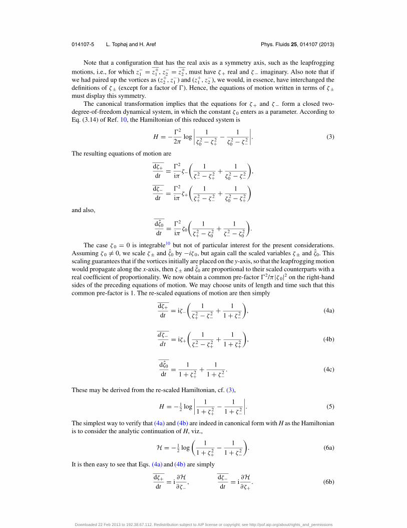
Level curves of H, Eq. (9a), are plotted in Fig. 3. (An equivalent figure also appears in Love’spaper5 at the end of Sec. 4.) Close to (X, Y) = (0, 0) these curves are circles X2 + Y2 ≈ h−1. Thislimit corresponds to h → ∞ or α → 1. We explore it further in Sec. VII.

In order for a curve (9b) to be closed, we must be able to solve (9b) for X when Y = 0. Thisimplies h > 1, and all the level curves (9b) for 1 < h < ∞ are closed and lead to leapfrogging

Downloaded 22 Feb 2013 to 192.38.67.112. Redistribution subject to AIP license or copyright; see http://pof.aip.org/about/rights_and_permissions

014107-7 L. Tophøj and H. Aref Phys. Fluids 25, 014107 (2013)

FIG. 3. Level curves of the Hamiltonian (9a).

motions. The lower limit h = 1 corresponds via (9d) to α = α0 = 3 − 2√

2. The range in α to beexplored, and to which we restrict attention, is then

3 − 2√

2 < α < 1. (10)

The determination of the lower limit of this range, α0 = σ 2, is a key result of the classical analyses.4, 5

See also Appendix B of Ref. 10 for a development of this material in a notation more similar to thatused here.

The period Tlf of the leapfrogging motion is given by Love5 in terms of elliptic integrals. In thepresent notation, and using the re-scaled time scale occurring in (7b), we have

Tl f = 26 α2

(1 − α)2

[E(k2)

(6α − α2 − 1)− K (k2)

(1 + α)2

], (11)

where k2 ≡ −24α(1 + α)2(1 − α)−4, and K and E are the complete elliptic integrals of the first andsecond kind, respectively.

IV. LINEAR STABILITY THEORY

Within the framework of Eqs. (4a) and (4b) we now consider perturbations to the periodic motiondescribed in Sec. III of the form

ζ+(t) = X (t) + ε[ξ+(t) + iη+(t)],

ζ−(t) = iY (t) + ε[ξ−(t) + iη−(t)],(12)

where ε is small and determines the size of the perturbation. All the functions X, Y, ξ±, and η±appearing here are real.

The most transparent way to derive the linearized perturbation equations is to start fromEqs. (6b) and expand to linear order. This gives

ξ+ − iη+ =

i∂2H∂ζ 2−

(ξ− + iη−) + i∂2H

∂ζ+∂ζ−(ξ+ + iη+),

ξ− − iη− =

i∂2H∂ζ 2+

(ξ+ + iη+) + i∂2H

∂ζ−∂ζ+(ξ− + iη−).

(13a)

The derivatives of H for the base solution, ζ+ = X, ζ− = iY, are

∂2H∂ζ 2−

= −∂2 H

∂Y 2= −HY Y ,

∂2H∂ζ 2+

= ∂2 H

∂ X2= HX X ,

∂2H∂ζ−∂ζ+

= −i∂2 H

∂ X∂Y= −i HXY .

(13b)

Downloaded 22 Feb 2013 to 192.38.67.112. Redistribution subject to AIP license or copyright; see http://pof.aip.org/about/rights_and_permissions

014107-8 L. Tophøj and H. Aref Phys. Fluids 25, 014107 (2013)

The components of the Hessian of H,

W =[

HX X HXYHY X HY Y

], (13c)

are, of course, all real. Explicitly,

HXY = HY X = 2XY

(X2 + Y 2)2(14a)

and

HX X = F(iY, X ), HY Y = −F(X, iY ), (14b)

where

F(Z1, Z2) = (1 + Z21)(3Z4

2 − Z21 Z2

2 + Z21 + Z2

2)

(1 + Z22)2(Z2

1 − Z22)2

. (14c)

Separating (13a) into real and imaginary parts, we now see that the perturbations decouple into twoindependent systems of equations for two variables each,

d

dt

[ξ+η−

]=

[HXY HY Y

−HX X −HXY

][ξ+η−

], (15a)

d

dt

[ξ−η+

]=

[HXY −HX X

HY Y −HXY

][ξ−η+

]. (15b)

We note that the coefficient matrix appearing in the second of these is[HXY −HX X

HY Y −HXY

]= WE,

where

E =[

0 −1

1 0

]. (16)

We note for later use that E2 = −1.The coefficient matrix appearing in Eq. (15a) is the transpose,[

HXY HY Y

−HX X −HXY

]= (WE)T = ETW = −EW.

The perturbation equations may thus be written in the form

d

dt

[ξ+η−

]= −EW

[ξ+η−

],

d

dt

[ξ−η+

]= WE

[ξ−η+

], (17)

where W is the Hessian (13c) and E is given by (16). The following explicit form is also important

d

dt

[ξ+η−

]= AT

[ξ+η−

],

d

dt

[ξ−η+

]= A

[ξ−η+

], (18a)

where

A = g(X, Y )

[XY f (iY, X )

f (X, iY ) −XY

], (18b)

Downloaded 22 Feb 2013 to 192.38.67.112. Redistribution subject to AIP license or copyright; see http://pof.aip.org/about/rights_and_permissions

014107-9 L. Tophøj and H. Aref Phys. Fluids 25, 014107 (2013)

with (cf. (14a))

g(X, Y ) = 2

(X2 + Y 2)2(18c)

and (cf. (14c))

f (Z1, Z2) = − 12 (Z2

1 − Z22)2 F(Z1, Z2). (18d)

Since g(X, Y) > 0 it may be absorbed into a rescaling of time via dτ = g(X, Y)dt.Formally the equations for (ξ+, η−) and (ξ−, η+) appear to be quite similar. There is, how-

ever, an important difference in terms of the physics between the two types of perturbations: The(ξ+, η−) perturbations preserve the discrete symmetry of the leapfrogging motion since ζ+ remainsreal and ζ− imaginary. In other words, infinitesimal perturbations of this kind must lead from oneleapfrogging motion to another. The (ξ−, η+) perturbations break the discrete symmetry. Hence, itis among these perturbations that we are to seek potential instabilities of leapfrogging motion.

By construction all perturbations (ξ+, η−) and (ξ−, η+) conserve the linear impulse ζ 0. Thechange in the analytic continuation of the Hamiltonian, H in Eq. (6a), for a general perturbation (12)is

δH =HX (ξ+ + iη+) − iHY (ξ− + iη−) =HXξ+ + HY η− + i(HXη+ − HY ξ−).

This is pure imaginary for perturbations with ξ+ = η− = 0 which shows that to leading order there isno change in the real part of H, in other words no change in H, Eq. (5), for a (ξ−, η+)-perturbation.The (ξ+, η−) perturbations will in general change H, the one exception being a perturbation along(HY, −HX), i.e., along (X , Y ). As we shall see, such perturbations are, in fact, solutions of thelinearized equations (15a).

Turning to the angular impulse, we have

I = �(|z+1 |2 + |z+

2 |2 − |z−1 |2 − |z−

2 |2)

= 2Re (ζ0ζ0 + ζ+ζ−),

according to Eq. (3.15) of Ref. 10. After rescaling this becomes I = 2Im(ζ0) + 2Re (ζ+ζ−). Thechange in I to first order in a perturbation of the form (12) is

δ I = 2Im(δζ0) + 2Re [−iY (ξ+ + iη+) + X (ξ− − iη−)]

= 2Im(δζ0) + 2(Xξ− + Yη+).

Thus, (ξ+, η−)-perturbations automatically preserve I. For (ξ−, η+)-perturbations we may preserveI if we agree to move the origin of coordinates, i.e., shift δζ0, such that δI = 0 for the perturbed initialstate. This is possible since ζ0 is simply twice the geometrical centroid of the four points where thevortices are located. Such a shift of the origin of coordinates has no effect on the value of the linearimpulse or the Hamiltonian, and the value of ζ0 does not enter into the dynamical equations for ζ±.Perturbations (ξ−, η+) along ( − Y, X) preserve I without need for shifting the origin of coordinates.

In summary, then, the perturbations (ξ−, η+) may be considered to take place at fixed values ofthe integrals of motion H and I. The perturbations (ξ+, η−) have a one-dimensional subspace thatdoes not conserve H.

V. FLOQUET ANALYSIS

Exploring the solutions to a system such as (17) leads us directly to Floquet theory.8 Due tothe periodic time dependence of the coefficient matrix, the behavior of solutions is not immediatelygiven by the local behavior of the solutions but rather by these solutions integrated over a period ofthe periodic motion. In effect, Floquet theory exploits the properties of the return map of the linearsystem integrated over a period of the motion whose stability is the object of study. We outline the

Downloaded 22 Feb 2013 to 192.38.67.112. Redistribution subject to AIP license or copyright; see http://pof.aip.org/about/rights_and_permissions

014107-10 L. Tophøj and H. Aref Phys. Fluids 25, 014107 (2013)

basics of the theory in order to establish our notation and emphasize what we need in the presentcase. The theory is treated in several places in the literature, e.g., Ref. 9.

We are dealing with a general system of ODEs of the form

ξ = Aξ , (19)

where ξ is a two-component vector and A a 2 × 2 matrix that is periodic in time. We shall apply thetheory to both the (ξ+, η−)- and (ξ−, η+)-perturbations of Sec. IV.

Construct a so-called fundamental matrix, �, by placing in the first column the solutionξ = (ξ, η) to (19) with initial condition (1, 0). In the second column place the solution with initialcondition (0, 1). The 2 × 2 matrix, � then satisfies the equation of evolution

� = A�. (20)

If A were constant in time, the solution would be easy enough,

�(t) = eAt�(0).

If A has eigenvalues μ1,2 with corresponding eigenvectors v(1,2), we have

Av(1,2) = μ1,2v(1,2), eAtv(1,2) = eμ1,2tv(1,2).

Hence, expanding ξ (0) along v(1,2), we obtain solution components that vary as eμ1,2t . If μ1,2 is pureimaginary, this leads to oscillatory evolution and thus spectral stability. On the other hand, if eitherof μ1,2 has a positive real part, we obtain unstable exponential growth of the perturbation.

For a time-periodic coefficient matrix we must proceed a bit differently: We exploit the period-icity of A with some period, T, to argue that if �(t) is a solution of (20), then �(t + T) will also be asolution. Next, since the space of solution vectors is two-dimensional, the columns of �(t + T) maybe expressed as linear combinations of the columns of �(t). In other words, there exists a matrix, M,called the monodromy matrix, such that

�(t + T ) = �(t)M. (21a)

With the two independent solutions we have chosen, we have �(0) = 1, the 2 × 2 unit matrix.Hence,

M = �(T ), �(t + T ) = �(t)�(T ). (21b)

If we wish to find the solution �(t) starting from general initial conditions �(0) = C, we haveonly to set �(t) = �(t)C. Then,

˙� = �C = A�C = A�,

so � satisfies the ODE, and by construction �(0) = C.A word of caution is necessary if �(t) becomes degenerate. Indeed, the term “fundamental

matrix” is usually reserved for the case when �(t) is non-degenerate. If the columns of �(t) becomeproportional, we must supplement the first column vector by a perpendicular vector to have a basisin the 2D space. The general theory is then somewhat modified. We continue with the assumptionthat �(t) is non-degenerate for 0 ≤ t ≤ T and return to the degenerate case as necessary.

Let v(±) be the eigenvectors of M corresponding to eigenvalues ρ±, respectively, i.e., Mv(±)

= ρ±v(±). It is important to emphasize that ρ± and v(±) are time independent quantities. Importantproperties of ρ± follow from the identity

d

dtdet � = TrA det �. (22)

This is, essentially, the relation for change of area in the 2D “flow” (20) and is, in any event, notdifficult to verify. In our case the coefficient matrix A is either WE or its transpose. Both havevanishing trace, so the right-hand side of (22) vanishes, and det � is invariant in time. Since det �(0)= 1, we have det M = det �(T) = 1 and thus ρ+ρ− = 1. Furthermore, in our case the vectors andmatrices are all real. In particular, the matrix M is real and its eigenvalues are thus either both real

Downloaded 22 Feb 2013 to 192.38.67.112. Redistribution subject to AIP license or copyright; see http://pof.aip.org/about/rights_and_permissions

014107-11 L. Tophøj and H. Aref Phys. Fluids 25, 014107 (2013)

(in which case they have the form ρ± = ρ±1 for some real ρ), or they are complex conjugates (inwhich case they have the form ρ± = e±iϕ for some angle ϕ).

Now consider the time-dependent vectors

ξ (±)(t) = �(t)v(±). (23)

We have

ξ(±) = �v(±) = A�v(±) = Aξ (±),

so the ξ (±)(t) are solutions to the ODEs (19). They have the initial values ξ (±)(0) = v(±). We see that

ξ (±)(t + T ) = �(t + T )v(±) =�(t)Mv(±) = ρ±�(t)v(±) = ρ±ξ (±)(t).

(24)

Thus, over a period of the coefficient matrix A the solutions ξ (±) are multiplied by ρ±, respectively.The general solution to the functional relation (24) is

ξ (±)(τ ) = ρτ/T± �±(τ ), (25)

where the arbitrary function �±(τ ) is periodic with period T and satisfies �±(0) = v(±). A directproof that �±(τ ) is periodic follows:

�±(τ + T ) = ρ−(τ+T )/T± ξ (±)(τ + T ) =

ρ−(τ+T )/T± ρ±ξ (±)(τ ) = ρ

−τ/T± ξ (±)(τ ) = �±(τ ).

The quantities ρ± are called the Floquet multipliers. One often sets ρ± = eμ±T , even thoughthe μ± are defined only up to multiples of 2π i/T. The μ± are called the Floquet exponents.

If ρ± are reciprocal real numbers, we have found a solution to (19) that grows exponentially.The underlying periodic motion from which these equations arose as linear perturbations is thenunstable. If ρ± are complex conjugates of modulus 1, the motion is linearly stable. A general initialcondition may be decomposed along v(±),

ξ (0) = a+v(+) + a−v(−)

and so will evolve according to

ξ (τ ) = a+ξ (+)(τ ) + a−ξ (−)(τ ) =a+ρ

τ/T+ �(+)(τ ) + a−ρ

τ/T− �(−)(τ ).

VI. FLOQUET ANALYSIS APPLIED TO THE EQUATIONS OF SEC. IV

We now adapt the general theory to our perturbation equations for the leapfrogging motion.First, concerning the period, T, of the coefficient matrices, −EW and WE in Eqs. (17), we see thatthis must be half the period of the leapfrogging motion Tlf, (11). We start at X = 0 and some finitevalue of Y. During an entire cycle of the leapfrogging motion X and Y vary through positive andnegative values. However, all the quantities HXX, HXY, HYY appearing in the coefficient matrices ofthe stability problem are even functions of X and Y. Hence, the period of the matrices is half theleapfrogging period.

Let us first consider the (ξ+, η−) equations even though these are not of primary interest tothe stability of leapfrogging. There is one obvious solution to these equations: If we differentiateEqs. (9e) once more with respect to time, we get

X = HY X X + HY Y Y , Y = −HX X X − HXY Y .

Written in matrix form, these equations show that (ξ+, η−) = (X , Y ) solve Eq. (15a).

Downloaded 22 Feb 2013 to 192.38.67.112. Redistribution subject to AIP license or copyright; see http://pof.aip.org/about/rights_and_permissions

014107-12 L. Tophøj and H. Aref Phys. Fluids 25, 014107 (2013)

The initial conditions (8) for leapfrogging imply

X (0) = −1

hY 30

, Y (0) = 0. (26)

This follows from (7b) or (7b′) and (9b) when the values from (8) are substituted. It is also clearfrom Fig. 3 that Y (0) vanishes and that X (0) is negative: The leapfrogging motion starts at a pointon the positive Y-axis of Fig. 3 as given by Eqs. (8). Since the level curves all have horizontaltangents on this axis, a (ξ+, η−)-perturbation of the initial condition that has only an X-componentwill simply move the phase point a bit forward or backward along the chosen trajectory, i.e., lead toa leapfrogging motion with the same value of the Hamiltonian. At time T the perturbation (X , Y )will have evolved into (X (T ), Y (T )) = (−X (0), 0). In other words, the (ξ+, η−)-perturbation that att = 0 is (1, 0) must, by linearity, have evolved into (−1, 0) at time t = T. This gives the first columnof the monodromy matrix M.

Next, from the determinant of the monodromy matrix being +1 we know that the lowerdiagonal element must also be −1. Hence, we have the form of the monodromy matrix for the (ξ+,η−) equations,

M =[

−1 A

0 −1

]. (27)

To find the number A, we proceed as follows. We consider a perturbation with initial condition (ξ+,η−) = (0, 1) of a state with initial condition (X, Y) = (0, Y0). This effectively takes us to anotherleapfrogging motion with initial condition (X, Y) = (0, Y0 + ε). Now, the leapfrogging period hasincreased by an amount dTlf = ε∂Tlf/∂Y0, which can be computed from (8) and (11). So after a time T= Tlf/2, the perturbed system will be a time dTlf/2 behind reaching its own half-period. To first orderin ε, the system will have evolved to (X, Y ) = (−dTl f X (T )/2,−Y0 − ε). Since the perturbationgoverned by (15a) must evolve in agreement with this result to linear order in ε, we will have(ξ+, η−) = (−dTl f X (T )/2,−1) at time T. Now, X (T ) = −X (0), so

A = 1

2

∂Tl f

∂Y0X (0), (28)

with A < 0. The result (27) and (28) shows that leapfrogging is always stable to (ξ+, η−) perturbations,as we have already argued. Also, it has been useful in checking our numerical procedure for evaluatingthe monodromy matrix.

It is straightforward to compute the Floquet exponents for the leapfrogging motion numerically.We have done so as a function of the parameter α in the initial condition (8). The classical leapfroggingsolution is required. This solution is given in terms of elliptic functions4, 5 that would, in any event,require numerical evaluation. It is therefore easier operationally, and just as accurate, to simplysolve the ODEs (7b) numerically along with the stability equations (17) such that X(t) and Y(t) areavailable at each step. We have used the Runge-Kutta 45 solver in the software package MATLAB R©

for this purpose.For the (ξ+, η−)-equations the numerical calculations simply verify the result in (27) and (28).

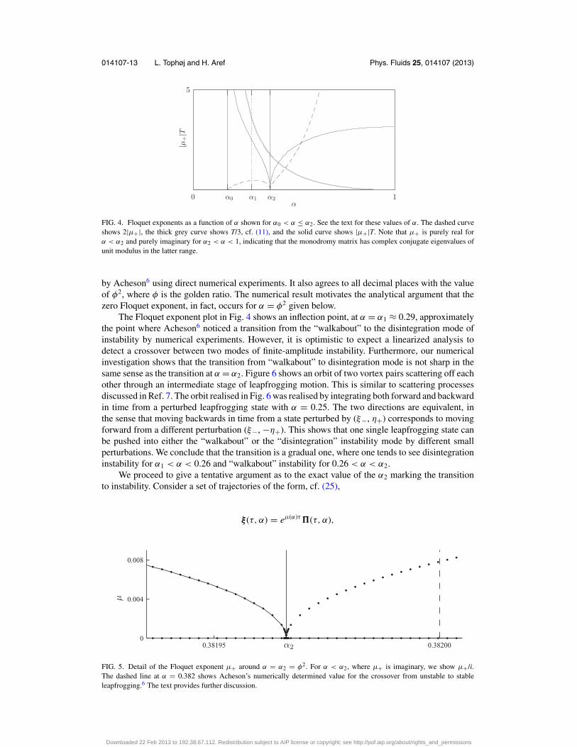
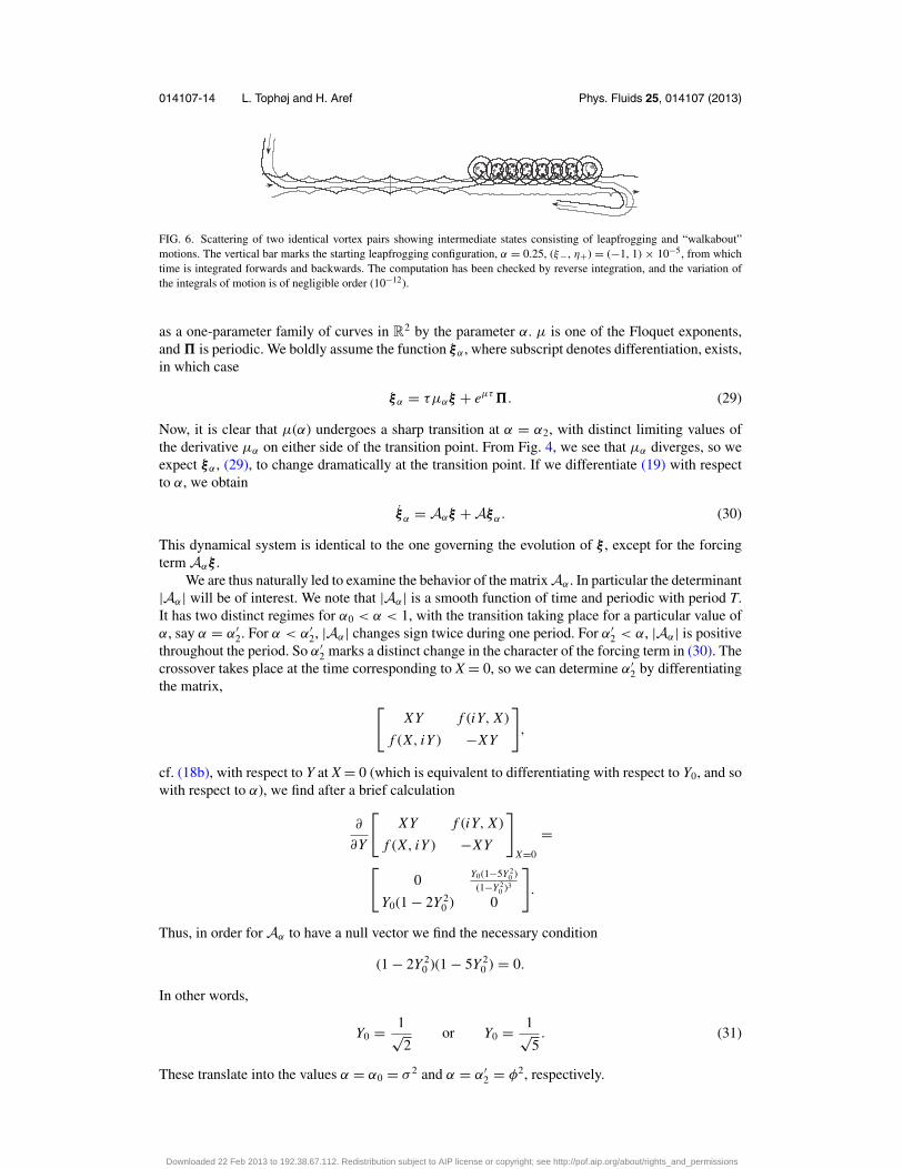
The Floquet analysis calculation for the (ξ−, η+)-equations is more interesting. The results havebeen collected in Fig. 4 which shows both μ+T and μ+ as functions of α. The relevant interval isα0 < α < 1. In this interval α0 = σ 2 ≈ 0.172 marks the onset of leapfrogging. Since T → ∞ asα → α0, we have plotted both μ+ and μ+T in Fig. 4 as functions of α. We see that for a range ofα, from the onset of leapfrogging to α = α2 ≈ 0.382, we have a real, positive Floquet exponentcorresponding to instability. The Floquet exponent μ+ vanishes at α = α0 and at α = α2. Beyondα = α2 the Floquet exponents become pure imaginary. The positive imaginary part, Im μ+T, hasbeen plotted in Fig. 4. Again, since T → 0 for α → 1, we have also plotted Im μ+. Figure 5 showsa magnification of the region close to α = α2. The vertical line is at α2 = 0.38197. . . , which wedetermine analytically in the sequel. This value agrees to three decimal places with the value found

Downloaded 22 Feb 2013 to 192.38.67.112. Redistribution subject to AIP license or copyright; see http://pof.aip.org/about/rights_and_permissions

014107-13 L. Tophøj and H. Aref Phys. Fluids 25, 014107 (2013)

|μ+|T

α

5

0 1α0 α1 α2

FIG. 4. Floquet exponents as a function of α shown for α0 < α ≤ α2. See the text for these values of α. The dashed curveshows 2|μ+|, the thick grey curve shows T/3, cf. (11), and the solid curve shows |μ+|T. Note that μ+ is purely real forα < α2 and purely imaginary for α2 < α < 1, indicating that the monodromy matrix has complex conjugate eigenvalues ofunit modulus in the latter range.

by Acheson6 using direct numerical experiments. It also agrees to all decimal places with the valueof φ2, where φ is the golden ratio. The numerical result motivates the analytical argument that thezero Floquet exponent, in fact, occurs for α = φ2 given below.

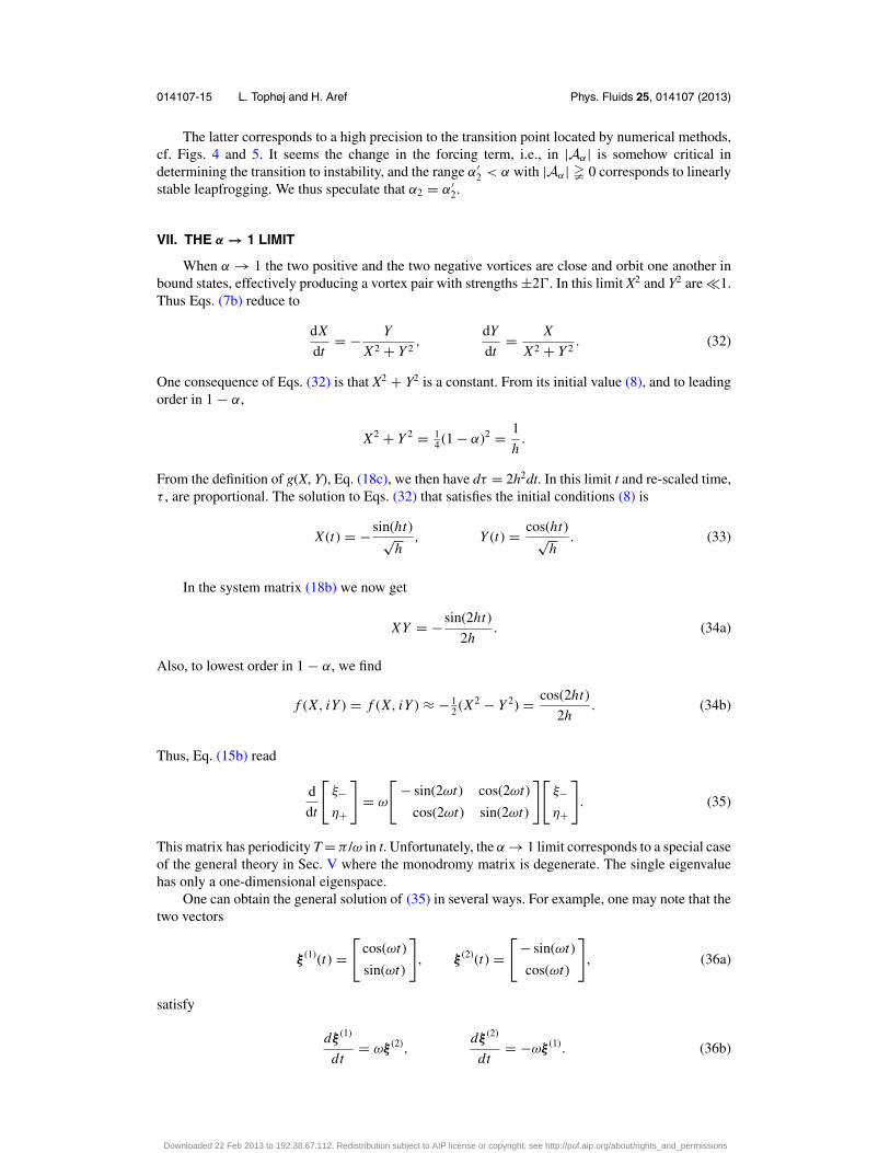
The Floquet exponent plot in Fig. 4 shows an inflection point, at α = α1 ≈ 0.29, approximatelythe point where Acheson6 noticed a transition from the “walkabout” to the disintegration mode ofinstability by numerical experiments. However, it is optimistic to expect a linearized analysis todetect a crossover between two modes of finite-amplitude instability. Furthermore, our numericalinvestigation shows that the transition from “walkabout” to disintegration mode is not sharp in thesame sense as the transition at α = α2. Figure 6 shows an orbit of two vortex pairs scattering off eachother through an intermediate stage of leapfrogging motion. This is similar to scattering processesdiscussed in Ref. 7. The orbit realised in Fig. 6 was realised by integrating both forward and backwardin time from a perturbed leapfrogging state with α = 0.25. The two directions are equivalent, inthe sense that moving backwards in time from a state perturbed by (ξ−, η+) corresponds to movingforward from a different perturbation (ξ−, −η+). This shows that one single leapfrogging state canbe pushed into either the “walkabout” or the “disintegration” instability mode by different smallperturbations. We conclude that the transition is a gradual one, where one tends to see disintegrationinstability for α1 < α < 0.26 and “walkabout” instability for 0.26 < α < α2.

We proceed to give a tentative argument as to the exact value of the α2 marking the transitionto instability. Consider a set of trajectories of the form, cf. (25),

ξ (τ, α) = eμ(α)τ�(τ, α),

0.38195 0.382000

0.004

0.008

μ

α2

FIG. 5. Detail of the Floquet exponent μ+ around α = α2 = φ2. For α < α2, where μ+ is imaginary, we show μ+/i.The dashed line at α = 0.382 shows Acheson’s numerically determined value for the crossover from unstable to stableleapfrogging.6 The text provides further discussion.

Downloaded 22 Feb 2013 to 192.38.67.112. Redistribution subject to AIP license or copyright; see http://pof.aip.org/about/rights_and_permissions

014107-14 L. Tophøj and H. Aref Phys. Fluids 25, 014107 (2013)

FIG. 6. Scattering of two identical vortex pairs showing intermediate states consisting of leapfrogging and “walkabout”motions. The vertical bar marks the starting leapfrogging configuration, α = 0.25, (ξ−, η+) = (−1, 1) × 10−5, from whichtime is integrated forwards and backwards. The computation has been checked by reverse integration, and the variation ofthe integrals of motion is of negligible order (10−12).

as a one-parameter family of curves in R2 by the parameter α. μ is one of the Floquet exponents,and � is periodic. We boldly assume the function ξα , where subscript denotes differentiation, exists,in which case

ξα = τμαξ + eμτ�. (29)

Now, it is clear that μ(α) undergoes a sharp transition at α = α2, with distinct limiting values ofthe derivative μα on either side of the transition point. From Fig. 4, we see that μα diverges, so weexpect ξα , (29), to change dramatically at the transition point. If we differentiate (19) with respectto α, we obtain

ξα = Aαξ + Aξα. (30)

This dynamical system is identical to the one governing the evolution of ξ , except for the forcingterm Aαξ .

We are thus naturally led to examine the behavior of the matrix Aα . In particular the determinant|Aα| will be of interest. We note that |Aα| is a smooth function of time and periodic with period T.It has two distinct regimes for α0 < α < 1, with the transition taking place for a particular value ofα, say α = α′

2. For α < α′2, |Aα| changes sign twice during one period. For α′

2 < α, |Aα| is positivethroughout the period. So α′

2 marks a distinct change in the character of the forcing term in (30). Thecrossover takes place at the time corresponding to X = 0, so we can determine α′

2 by differentiatingthe matrix, [

XY f (iY, X )

f (X, iY ) −XY

],

cf. (18b), with respect to Y at X = 0 (which is equivalent to differentiating with respect to Y0, and sowith respect to α), we find after a brief calculation

∂

∂Y

[XY f (iY, X )

f (X, iY ) −XY

]X=0

=[

0 Y0(1−5Y 20 )

(1−Y 20 )3

Y0(1 − 2Y 20 ) 0

].

Thus, in order for Aα to have a null vector we find the necessary condition

(1 − 2Y 20 )(1 − 5Y 2

0 ) = 0.

In other words,

Y0 = 1√2

or Y0 = 1√5. (31)

These translate into the values α = α0 = σ 2 and α = α′2 = φ2, respectively.

Downloaded 22 Feb 2013 to 192.38.67.112. Redistribution subject to AIP license or copyright; see http://pof.aip.org/about/rights_and_permissions

014107-15 L. Tophøj and H. Aref Phys. Fluids 25, 014107 (2013)

The latter corresponds to a high precision to the transition point located by numerical methods,cf. Figs. 4 and 5. It seems the change in the forcing term, i.e., in |Aα| is somehow critical indetermining the transition to instability, and the range α′

2 < α with |Aα| � 0 corresponds to linearlystable leapfrogging. We thus speculate that α2 = α′

2.

VII. THE α → 1 LIMIT

When α → 1 the two positive and the two negative vortices are close and orbit one another inbound states, effectively producing a vortex pair with strengths ±2�. In this limit X2 and Y2 are 1.Thus Eqs. (7b) reduce to

dX

dt= − Y

X2 + Y 2,

dY

dt= X

X2 + Y 2. (32)

One consequence of Eqs. (32) is that X2 + Y2 is a constant. From its initial value (8), and to leadingorder in 1 − α,

X2 + Y 2 = 14 (1 − α)2 = 1

h.

From the definition of g(X, Y), Eq. (18c), we then have dτ = 2h2dt. In this limit t and re-scaled time,τ , are proportional. The solution to Eqs. (32) that satisfies the initial conditions (8) is

X (t) = − sin(ht)√h

, Y (t) = cos(ht)√h

. (33)

In the system matrix (18b) we now get

XY = − sin(2ht)

2h. (34a)

Also, to lowest order in 1 − α, we find

f (X, iY ) = f (X, iY ) ≈ − 12 (X2 − Y 2) = cos(2ht)

2h. (34b)

Thus, Eq. (15b) read

d

dt

[ξ−η+

]= ω

[− sin(2ωt) cos(2ωt)

cos(2ωt) sin(2ωt)

][ξ−η+

]. (35)

This matrix has periodicity T = π /ω in t. Unfortunately, the α → 1 limit corresponds to a special caseof the general theory in Sec. V where the monodromy matrix is degenerate. The single eigenvaluehas only a one-dimensional eigenspace.

One can obtain the general solution of (35) in several ways. For example, one may note that thetwo vectors

ξ (1)(t) =[

cos(ωt)

sin(ωt)

], ξ (2)(t) =

[− sin(ωt)

cos(ωt)

], (36a)

satisfy

dξ (1)

dt= ωξ (2),

dξ (2)

dt= −ωξ (1). (36b)

Downloaded 22 Feb 2013 to 192.38.67.112. Redistribution subject to AIP license or copyright; see http://pof.aip.org/about/rights_and_permissions

014107-16 L. Tophøj and H. Aref Phys. Fluids 25, 014107 (2013)

Further, if the matrix on the right-hand side of (35), without the factor ω, is designated A, then

Aξ (1) = ξ (2), Aξ (2) = ξ (1). (36c)

If we posit that a vector, ξ (t), solves (35), and if we expand it in terms of ξ (1,2) as

ξ (t) = a(t)ξ (1)(t) + b(t)ξ (2)(t),

with time-dependent coefficient a(t) and b(t), we find the conditions

da

dt= −2ωb,

db

dt= 0.

This shows that such a decomposition requires b to be a constant, b = C1, and a(t) = −2ωC1t + C2,where C2 is a second constant. In particular, a and b cannot both be constants, but there must be asecular term in the expansion.

The general solution is[ξ−η+

]= (C2 − 2C1ωt)

[cos ωt

sin ωt

]+ C1

[− sin ωt

cos ωt

], (37a)

with constants C1 and C2 chosen to match initial conditions. The initial conditions ξ− = 1, η+ = 0correspond to C1 = 0, C2 = 1, the initial conditions ξ− = 0, η+ = 1 to C1 = 1, C2 = 0. At t = T= π /ω these have evolved to (−1, 0) and (2π , −1), respectively. Thus,

M = �(T ) =[

−1 2π

0 −1

]. (37b)

The eigenvalue ρ = −1 has a one-dimensional eigenspace. The secular term in (37a) reflects thisdegeneracy of the monodromy matrix.

VIII. CONCLUSIONS

The stability of leapfrogging motion has been investigated using Floquet theory. By studyingthe Floquet exponents of the linearized perturbation equations, we have confirmed the numericalresults of Acheson.6 Furthermore, we have argued analytically that the transition to instabilityoccurs when the pair size ratio is exactly α = φ2, the square of the golden ratio, in agreementwith numerical results. The linear analysis does not explain the transition between the “walkabout”and “disintegration” instability modes identified by Acheson,6 but our numerical calculations hasrevealed that the transition is gradual rather than sharp, with both modes accessible by perturbationof a single leapfrogging motion. An example was given of leapfrogging occurring as an intermediatestate in the chaotic scattering of vortex pairs.7 We mention that the advection of particles by theperiodic flow due to leapfrogging is chaotic. This has been explored by Pentek et al.11

ACKNOWLEDGMENTS

The presented work was supported in part by a Niels Bohr Visiting Professorship at the TechnicalUniversity of Denmark sponsored by the Danish National Research Foundation. This paper isdedicated to the memory of Hassan Aref, who passed away during its preparation. He was a friendand a great inspiration.

1 H. von Helmholtz, “Uber Integrale der hydrodynamischen Gleichungen, welche den Wirbelbewegungen entsprechen,”J. Reine Angew. Math. 55, 25–55 (1858); P. G. Tait, “On integrals of the hydrodynamical equations, which expressvortex-motion,” Philos. Mag. 33(4), 485–512 (1867) (in English).

2 H. Yamada and T. Matsui, “Preliminary study of mutual slip-through of a pair of vortices,” Phys. Fluids 21, 292–294(1978).

3 B. N. Shashikanth and J. E. Marsden, “Leapfrogging vortex rings: Hamiltonian structure, geometric phases and discretereduction,” Fluid Dyn. Res. 33, 333–356 (2003).

Downloaded 22 Feb 2013 to 192.38.67.112. Redistribution subject to AIP license or copyright; see http://pof.aip.org/about/rights_and_permissions

014107-17 L. Tophøj and H. Aref Phys. Fluids 25, 014107 (2013)

4 W. Grobli, “Spezielle probleme uber die Bewegung geradliniger paralleler Wirbelfaden,” Vierteljahrsschr. Naturforsch.Ges. Zur. 22, 37–81, 129–165 (1877).

5 A. E. H. Love, “On the motion of paired vortices with a common axis,” Proc. London Math. Soc. 25, 185–194 (1893).6 D. J. Acheson, “Instability of vortex leapfrogging,” Eur. J. Phys. 21, 269–273 (2000).7 L. Tophøj and H. Aref, “Chaotic scattering of two identical point vortex pairs revisited,” Phys. Fluids 20, 093605 (2008).8 G. Floquet, “Sur les equations differentielles lineaires a coefficients periodiques,” Ann. Sci. Ec. Normale Super. (2nd

series) 12, 47–88 (1883).9 A. H. Nayfeh and B. Balachandran, Applied Nonlinear Dynamics–Analytical, Computational and Experimental Methods

(Wiley, New York, 1995).10 B. Eckhardt and H. Aref, “Integrable and chaotic motions of four vortices II. Collision dynamics of vortex pairs,” Philos.

Trans. R. Soc. London, Ser. A 326, 655–696 (1988).11 A. Pentek, T. Tel, and T. Toroczkai, “Chaotic advection in the velocity field of leapfrogging vortex pairs,” J. Phys. A 28,

2191–2216 (1995).

Downloaded 22 Feb 2013 to 192.38.67.112. Redistribution subject to AIP license or copyright; see http://pof.aip.org/about/rights_and_permissions