Newcastle University ePrints - eprint.ncl.ac.uk

Hietala N, Hänninen R, Salman H, Barenghi CF.

Leapfrogging Kelvin waves.

Physical Review Fluids 2016, 1(8), 084501.

Copyright:

©2017 American Physical Society. All rights reserved. This is the authors’ accepted manuscript of an

article that was published in its final definitive form by American Physical Society, 2016.

DOI link to article:

https://doi.org/10.1103/PhysRevFluids.1.084501

Date deposited:

30/03/2017

Leapfrogging Kelvin wavesN. Hietala,1, a) R. Hänninen,1 H. Salman,2 and C. F. Barenghi31)Low Temperature Laboratory, Department of Applied Physics, Aalto University, PO Box 15100,FI-00076 AALTO, Finland2)School of Mathematics, University of East Anglia, Norwich Research Park, Norwich NR4 7TJ,United Kingdom3)Joint Quantum Centre Durham-Newcastle, School of Mathematics and Statistics, Newcastle University,Newcastle upon Tyne NE1 7RU, United Kingdom

(Dated: November 23, 2016)

Two vortex rings can form a localized configuration whereby they continually pass through oneanother in an alternating fashion. This phenomenon is called leapfrogging. Using parameterssuitable for superfluid helium-4, we describe a recurrence phenomenon that is similar to leapfrog-ging, which occurs for two coaxial straight vortex filaments with the same Kelvin wave mode. Forsmall-amplitude Kelvin waves we demonstrate that our full Biot-Savart simulations closely followpredictions obtained from a simplified model that provides an analytical approximation developedfor nearly parallel vortices. Our results are also relevant to thin-cored helical vortices in classicalfluids.

PACS numbers: 47.32.C-, 67.25.dk, 47.37.+q

I. INTRODUCTION

The mathematical foundation of vortex dynamics was laid down by Helmholtz1,2, who subsequentlyapplied his theory to study the propagation of vortex rings. In his work, he suggested that two vortexrings moving along the same axis would thread each other in an alternating fashion. The study of vortexrings was also taken up by Lord Kelvin who contributed significantly to our understanding of the motion ofvortices in general. Following the works of Helmholtz and Kelvin, the leapfrogging motion of vortex ringshas been studied in more detail for classical fluids3–5 and also for superfluids6,7.

Leapfrogging of vortex rings is an interesting example of a recurrence phenomenon involving two vortices.In this work, we will give another example of leapfrogging, which can resemble the motion of two coaxialvortex rings. Part of our motivation is to understand the interaction of Kelvin waves on quantized superfluidvortices. It has been argued that Kelvin waves, which are helical perturbations of a straight vortex, areimportant for the energy dissipation in superfluid turbulence at very low temperatures8–10. However, a largebody of analytical results and a number of numerical studies rely on the simplifying assumption of neglectingthe interaction of the Kelvin waves between different vortex filaments and focus on how Kelvin waves evolveon a single filament. Despite this, the justification of these assumptions on which many of these theories arebased is not fully established.

In this work we will uncover a novel type of interaction between adjacent vortex filaments that can play animportant role in our understanding of how energy is transferred across different length scales. We note thatsome Kelvin wave phenomena bear resemblance to the motion of vortex rings. For example, a superfluidvortex ring experiencing a counterflow (the relative velocity of normal fluid and superfluid11) through itwill either shrink or grow depending on the direction of the counterflow. Similarly, the amplitude of aKelvin wave will either decrease or increase depending on the amount of the counterflow along the vortexaxis12. On the other hand, a vortex with a large-amplitude Kelvin wave has a shape that correspondsto a tightly wound helix that, in some approximate sense, bears resemblance to a stacked row of vortexrings. Although the correspondence is not exact, in this work we propose that two stacked rows of vortexrings mimics the motion of two vortices with large-amplitude Kelvin waves. It turns out that this analogyprovides a qualitative understanding of the observed dynamics. Interestingly, we will show that a form ofvortex leapfrogging persists even when the Kelvin wave amplitudes are small.

Aside from their importance for superfluid turbulence, helical vortices are also important for classicalfluid dynamics. For example, the wake behind rotors can be treated as one or many interlaced helical

a)Electronic mail: niklas.hietala@aalto.fi

arX

iv:1

603.

0640

3v2

[ph

ysic

s.fl

u-dy

n] 2

2 N

ov 2

016

2

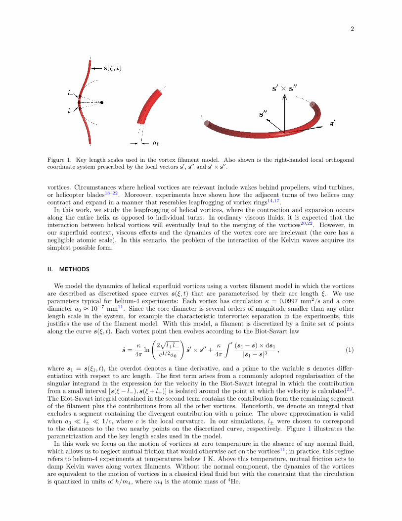
Figure 1. Key length scales used in the vortex filament model. Also shown is the right-handed local orthogonalcoordinate system prescribed by the local vectors s′, s′′ and s′ × s′′.

vortices. Circumstances where helical vortices are relevant include wakes behind propellers, wind turbines,or helicopter blades13–22. Moreover, experiments have shown how the adjacent turns of two helices maycontract and expand in a manner that resembles leapfrogging of vortex rings14,17.

In this work, we study the leapfrogging of helical vortices, where the contraction and expansion occursalong the entire helix as opposed to individual turns. In ordinary viscous fluids, it is expected that theinteraction between helical vortices will eventually lead to the merging of the vortices20,22. However, inour superfluid context, viscous effects and the dynamics of the vortex core are irrelevant (the core has anegligible atomic scale). In this scenario, the problem of the interaction of the Kelvin waves acquires itssimplest possible form.

II. METHODS

We model the dynamics of helical superfluid vortices using a vortex filament model in which the vorticesare described as discretized space curves s(ξ, t) that are parameterised by their arc length ξ. We useparameters typical for helium-4 experiments: Each vortex has circulation κ = 0.0997 mm2/s and a corediameter a0 ≈ 10−7 mm11. Since the core diameter is several orders of magnitude smaller than any otherlength scale in the system, for example the characteristic intervortex separation in the experiments, thisjustifies the use of the filament model. With this model, a filament is discretized by a finite set of pointsalong the curve s(ξ, t). Each vortex point then evolves according to the Biot-Savart law

s =κ

4πln

(2√l+l−

e1/2a0

)s′ × s′′ +

κ

4π

∫ ′ (s1 − s)× ds1|s1 − s|3

, (1)

where s1 = s(ξ1, t), the overdot denotes a time derivative, and a prime to the variable s denotes differ-entiation with respect to arc length. The first term arises from a commonly adopted regularisation of thesingular integrand in the expression for the velocity in the Biot-Savart integral in which the contributionfrom a small interval [s(ξ − l−), s(ξ + l+)] is isolated around the point at which the velocity is calculated23.The Biot-Savart integral contained in the second term contains the contribution from the remaining segmentof the filament plus the contributions from all the other vortices. Henceforth, we denote an integral thatexcludes a segment containing the divergent contribution with a prime. The above approximation is validwhen a0 � l± � 1/c, where c is the local curvature. In our simulations, l± were chosen to correspondto the distances to the two nearby points on the discretized curve, respectively. Figure 1 illustrates theparametrization and the key length scales used in the model.

In this work we focus on the motion of vortices at zero temperature in the absence of any normal fluid,which allows us to neglect mutual friction that would otherwise act on the vortices11; in practice, this regimerefers to helium-4 experiments at temperatures below 1 K. Above this temperature, mutual friction acts todamp Kelvin waves along vortex filaments. Without the normal component, the dynamics of the vorticesare equivalent to the motion of vortices in a classical ideal fluid but with the constraint that the circulationis quantized in units of h/m4, where m4 is the atomic mass of 4He.

3

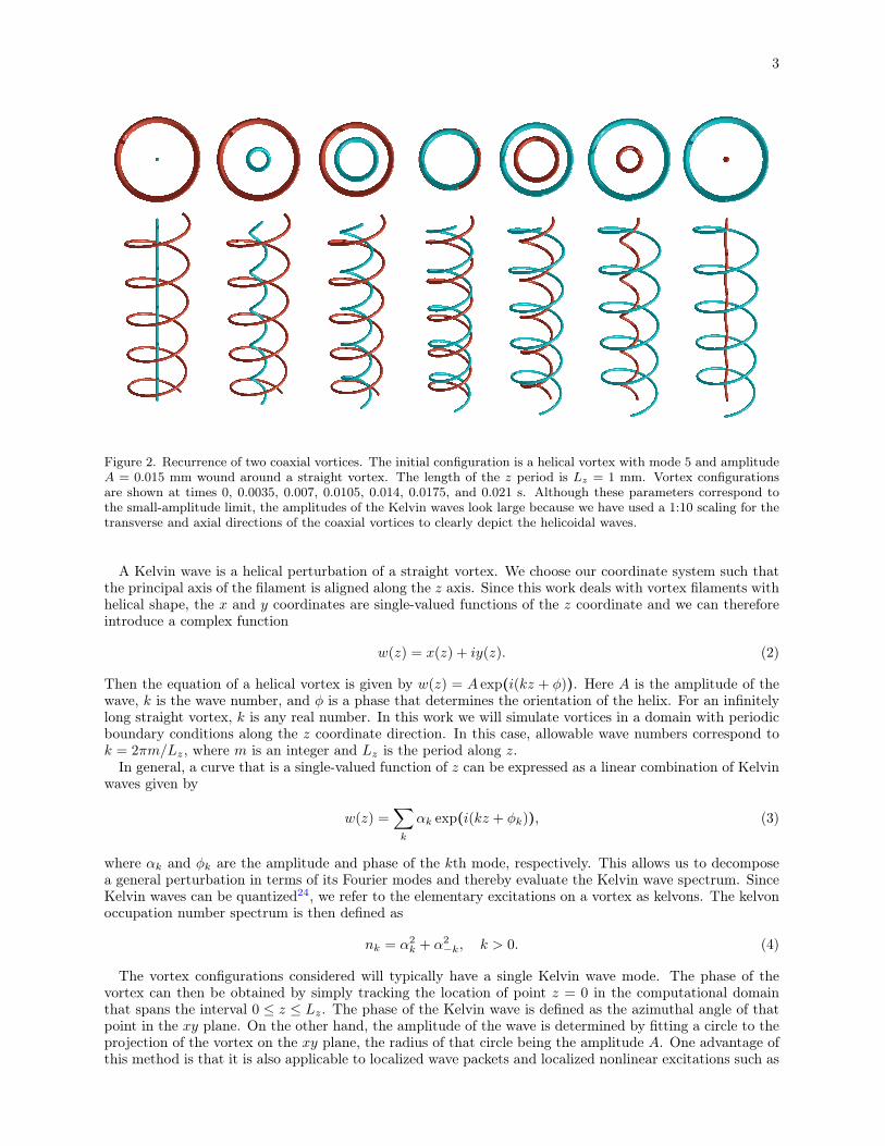
Figure 2. Recurrence of two coaxial vortices. The initial configuration is a helical vortex with mode 5 and amplitudeA = 0.015 mm wound around a straight vortex. The length of the z period is Lz = 1 mm. Vortex configurationsare shown at times 0, 0.0035, 0.007, 0.0105, 0.014, 0.0175, and 0.021 s. Although these parameters correspond tothe small-amplitude limit, the amplitudes of the Kelvin waves look large because we have used a 1:10 scaling for thetransverse and axial directions of the coaxial vortices to clearly depict the helicoidal waves.

A Kelvin wave is a helical perturbation of a straight vortex. We choose our coordinate system such thatthe principal axis of the filament is aligned along the z axis. Since this work deals with vortex filaments withhelical shape, the x and y coordinates are single-valued functions of the z coordinate and we can thereforeintroduce a complex function

w(z) = x(z) + iy(z). (2)

Then the equation of a helical vortex is given by w(z) = A exp(i(kz + φ)). Here A is the amplitude of thewave, k is the wave number, and φ is a phase that determines the orientation of the helix. For an infinitelylong straight vortex, k is any real number. In this work we will simulate vortices in a domain with periodicboundary conditions along the z coordinate direction. In this case, allowable wave numbers correspond tok = 2πm/Lz, where m is an integer and Lz is the period along z.

In general, a curve that is a single-valued function of z can be expressed as a linear combination of Kelvinwaves given by

w(z) =∑k

αk exp(i(kz + φk)), (3)

where αk and φk are the amplitude and phase of the kth mode, respectively. This allows us to decomposea general perturbation in terms of its Fourier modes and thereby evaluate the Kelvin wave spectrum. SinceKelvin waves can be quantized24, we refer to the elementary excitations on a vortex as kelvons. The kelvonoccupation number spectrum is then defined as

nk = α2k + α2

−k, k > 0. (4)

The vortex configurations considered will typically have a single Kelvin wave mode. The phase of thevortex can then be obtained by simply tracking the location of point z = 0 in the computational domainthat spans the interval 0 ≤ z ≤ Lz. The phase of the Kelvin wave is defined as the azimuthal angle of thatpoint in the xy plane. On the other hand, the amplitude of the wave is determined by fitting a circle to theprojection of the vortex on the xy plane, the radius of that circle being the amplitude A. One advantage ofthis method is that it is also applicable to localized wave packets and localized nonlinear excitations such as

4

t (s)0 0.05 0.1 0.15 0.2

∆φ

- π

- π/2

0

π/2

πsimulationmodel

t (s)0 0.05 0.1 0.15 0.2

A (

mm

)

0

0.005

0.01

0.015

0.02

0.025 vortex 1: simulationvortex 1: modelvortex 2: simulationvortex 2: model

t (s)0 5 10 15 20

∆φ

- π

- π/2

0

π/2

πsimulationmodel

t (s)0 5 10 15 20

A (

mm

)

0

0.05

0.1

0.15

0.2

0.25(a)

(b)

(c)

(d)

vortex 1: simulationvortex 1: modelvortex 2: simulationvortex 2: model

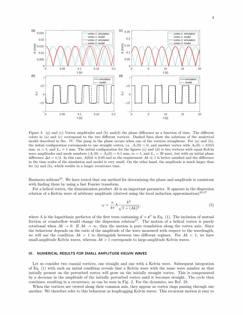
Figure 3. (a) and (c) Vortex amplitudes and (b) and(d) the phase difference as a function of time. The differentcolors in (a) and (c) correspond to the two different vortices. Dashed lines show the solutions of the analyticalmodel described in Sec. IV. The jump in the phase occurs when one of the vortices straightens. For (a) and (b),the initial configuration corresponds to one straight vortex, i.e. A1(0) = 0, and another vortex with A2(0) = 0.015mm, m = 5, and Lz = 1 mm. The initial configuration for the figures (c) and (d) is two vortices with equal Kelvinwave amplitudes and mode numbers (A1(0) = A2(0) = 0.1 mm, m = 1, and Lz = 20 mm), but with an initial phasedifference ∆φ = π/2. In this case, A(0)k ≈ 0.03 and so the requirement Ak � 1 is better satisfied and the differencein the time scales of the simulation and model is very small. On the other hand, the amplitude is much larger thanfor (a) and (b), which results in a longer recurrence time.

Hasimoto solitons25. We have tested that our method for determining the phase and amplitude is consistentwith finding them by using a fast Fourier transform.

For a helical vortex, the dimensionless product Ak is an important parameter. It appears in the dispersionrelation of a Kelvin wave of arbitrary amplitude (derived using the local induction approximation)26,27

ω =κ

4πΛ

k2√1 + (Ak)2

, (5)

where Λ is the logarithmic prefactor of the first term containing s′× s′′ in Eq. (1). The inclusion of mutualfriction or counterflow would change the dispersion relation27. The motion of a helical vortex is purelyrotational when Ak → 0. If Ak → ∞, then the motion is pure translation along the vortex axis. Sincethe behaviour depends on the ratio of the amplitude of the wave measured with respect to the wavelength,we will use the condition Ak = 1 to distinguish between two different regimes. For Ak < 1, we havesmall-amplitude Kelvin waves, whereas Ak > 1 corresponds to large-amplitude Kelvin waves.

III. NUMERICAL RESULTS FOR SMALL AMPLITUDE KELVIN WAVES

Let us consider two coaxial vortices, one straight and one with a Kelvin wave. Subsequent integrationof Eq. (1) with such an initial condition reveals that a Kelvin wave with the same wave number as thatinitially present on the perturbed vortex will grow on the initially straight vortex. This is compensatedby a decrease in the amplitude of the initially perturbed vortex until it becomes straight. The cycle thencontinues, resulting in a recurrence, as can be seen in Fig. 2. For the dynamics, see Ref. 28.

When the vortices are viewed along their common axis, they appear as vortex rings passing through oneanother. We therefore refer to this behaviour as leapfrogging Kelvin waves. This recurrent motion is easy to

5

t (s)0 0.1 0.2 0.3 0.4 0.5 0.6

A (m

m)

0

0.005

0.01

0.015

m10 0 10 2

n k

10 -20

10 -10

10 0

0.02

-0.02-0.02

1

00.02

0.02

-0.02-0.02

1

00.02

(a) (b)

(c)

Figure 4. Leapfrogging of Kelvin waves (for m = 5) with random perturbations added to the initial configuration ofthe helical vortex. (a) Initial configuration. (b) Configuration (inset) and the kelvon occupation spectrum at t = 0.6s. After more than ten recurrence periods, the initial Kelvin mode still clearly dominates. (c) Amplitudes of thewaves as a function of time. It is apparent that the recurrence is practically unaffected by the noise.

see if we consider the amplitudes of the vortices as functions of time (see Fig. 3). We note that the exchangeof energy that is associated with the hopping of the Kelvin wave from one vortex onto the other and viceversa arises from the intrinsic nonlocal dynamics of the Biot-Savart law. The phenomena we observe cannotbe described using the so-called local induction approximation, which retains only the first term in Eq. (1).

During the evolution, the momentum (or, more precisely, the impulse) of the vortices defined as

I =ρsκ

2

∫s× ds. (6)

is conserved. Here ρs is the superfluid density and the integral is performed over the interval 0 ≤ z ≤ Lz.The z component of the momentum (i.e., along the vortex) is proportional to the product of the area of theprojection of the vortex line onto the xy plane times the mode number, i.e., the number of times the vortexwinds around the axis within one period. From this we can determine the instants when the amplitudes ofthe Kelvin waves of each vortex are equal. This should occur when A = A(0)/

√2. This is confirmed in the

results presented in Fig. 3.We have found that the leapfrogging motion of Kelvin waves is a robust effect, which occurs even if we

add some random white noise to the initial configuration. Figure 4 shows the evolution of a Kelvin waveon a vortex to which we added some noise with magnitude equal to 2 % of the original amplitude. It isclear that even after more than ten recurrence periods we can still see the initial Kelvin mode, confirmingthe persistence of the leapfrogging behaviour for initially perturbed Kelvin waves. We have also tested thestability to sideband modes (m − 1 and m + 1) with small amplitudes and found that such a perturbationdid not destroy the recurrence of the leapfrogging.

We note that for the leapfrogging to take place, it is not necessary for one of the vortices to be initiallystraight. Leapfrogging occurs whenever the coaxial vortices have the same Kelvin wave mode. If thevortices initially have equal amplitudes (an example is shown in Fig. 5), then the minimum and maximum

6

t (s)0 0.05 0.1 0.15

∆φ

- π

- π/2

0

π/2

π

0.01

-0.01-0.01

1

00.01

t (s)0 0.05 0.1 0.15

A (m

m)

× 10 -3

4

6

8

10

12

14(b)

(a)

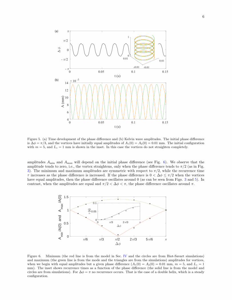
Figure 5. (a) Time development of the phase difference and (b) Kelvin wave amplitudes. The initial phase differenceis ∆φ = π/3, and the vortices have initially equal amplitudes of A1(0) = A2(0) = 0.01 mm. The initial configurationwith m = 5, and Lz = 1 mm is shown in the inset. In this case the vortices do not straighten completely.

amplitudes Amin and Amax will depend on the initial phase difference (see Fig. 6). We observe that theamplitude tends to zero, i.e., the vortex straightens, only when the phase difference tends to π/2 (as in Fig.3). The minimum and maximum amplitudes are symmetric with respect to π/2, while the recurrence timeτ increases as the phase difference is increased. If the phase difference is 0 < ∆φ ≤ π/2 when the vorticeshave equal amplitudes, then the phase difference oscillates around 0 (as can be seen from Figs. 3 and 5). Incontrast, when the amplitudes are equal and π/2 < ∆φ < π, the phase difference oscillates around π.

∆φ

π/6 π/3 π/2 2π/3 5π/6 πAm

in/A

(0)

and

A

max

/A(0

)

0

0.5

1

1.5

∆φ

0 π/3 2π/3 π

τ (

s)

0

0.05

0.1

Figure 6. Minimum (the red line is from the model in Sec. IV and the circles are from Biot-Savart simulations)and maximum (the green line is from the mode and the triangles are from the simulations) amplitudes for vortices,when we begin with equal amplitudes but a given phase difference (A1(0) = A2(0) = 0.01 mm, m = 5, and Lz = 1mm). The inset shows recurrence times as a function of the phase difference (the solid line is from the model andcircles are from simulations). For ∆φ = π no recurrence occurs. That is the case of a double helix, which is a steadyconfiguration.

7

It is remarkable that throughout the leapfrogging process, the two helical vortices do not cross andreconnect. If the phase difference is small when the vortices have equal amplitudes, they come really close toeach other (∆φ cannot be exactly zero, since then the vortices would coincide). Even then the reconnectiondoes not happen easily. This is because the vortices are locally parallel and any reconnection would increasethe vortex length and is thus not energetically favorable.

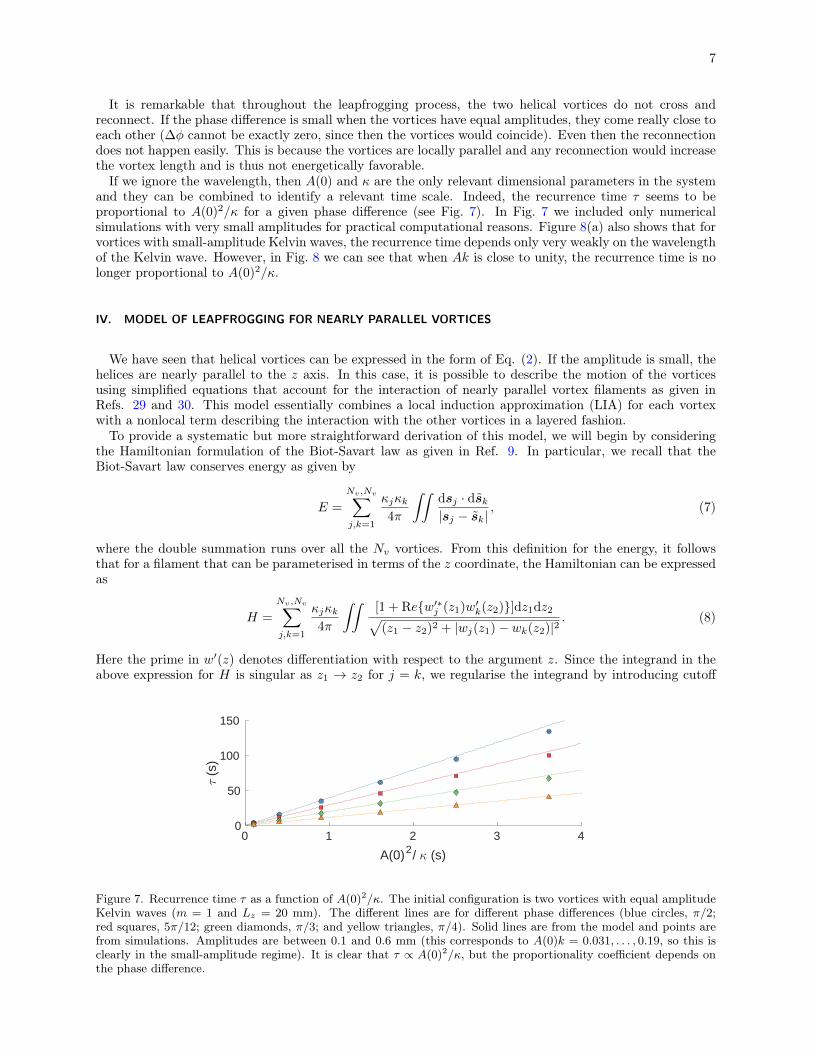
If we ignore the wavelength, then A(0) and κ are the only relevant dimensional parameters in the systemand they can be combined to identify a relevant time scale. Indeed, the recurrence time τ seems to beproportional to A(0)2/κ for a given phase difference (see Fig. 7). In Fig. 7 we included only numericalsimulations with very small amplitudes for practical computational reasons. Figure 8(a) also shows that forvortices with small-amplitude Kelvin waves, the recurrence time depends only very weakly on the wavelengthof the Kelvin wave. However, in Fig. 8 we can see that when Ak is close to unity, the recurrence time is nolonger proportional to A(0)2/κ.

IV. MODEL OF LEAPFROGGING FOR NEARLY PARALLEL VORTICES

We have seen that helical vortices can be expressed in the form of Eq. (2). If the amplitude is small, thehelices are nearly parallel to the z axis. In this case, it is possible to describe the motion of the vorticesusing simplified equations that account for the interaction of nearly parallel vortex filaments as given inRefs. 29 and 30. This model essentially combines a local induction approximation (LIA) for each vortexwith a nonlocal term describing the interaction with the other vortices in a layered fashion.

To provide a systematic but more straightforward derivation of this model, we will begin by consideringthe Hamiltonian formulation of the Biot-Savart law as given in Ref. 9. In particular, we recall that theBiot-Savart law conserves energy as given by

E =

Nv,Nv∑j,k=1

κjκk4π

∫∫dsj · dsk|sj − sk|

, (7)

where the double summation runs over all the Nv vortices. From this definition for the energy, it followsthat for a filament that can be parameterised in terms of the z coordinate, the Hamiltonian can be expressedas

H =

Nv,Nv∑j,k=1

κjκk4π

∫∫[1 + Re{w′∗j (z1)w′k(z2)}]dz1dz2√(z1 − z2)2 + |wj(z1)− wk(z2)|2

. (8)

Here the prime in w′(z) denotes differentiation with respect to the argument z. Since the integrand in theabove expression for H is singular as z1 → z2 for j = k, we regularise the integrand by introducing cutoff

A(0)2/ κ (s)

0 1 2 3 4

τ (s

)

0

50

100

150

Figure 7. Recurrence time τ as a function of A(0)2/κ. The initial configuration is two vortices with equal amplitudeKelvin waves (m = 1 and Lz = 20 mm). The different lines are for different phase differences (blue circles, π/2;red squares, 5π/12; green diamonds, π/3; and yellow triangles, π/4). Solid lines are from the model and points arefrom simulations. Amplitudes are between 0.1 and 0.6 mm (this corresponds to A(0)k = 0.031, . . . , 0.19, so this isclearly in the small-amplitude regime). It is clear that τ ∝ A(0)2/κ, but the proportionality coefficient depends onthe phase difference.

8

scales l± as described in Sec. II such that a0 � l± � 1/c. This choice of the cutoff scale, which has alsobeen described in Ref. 23, leads to

H ≈∑Nv

j=1

κ2j

2π ln

(2√l+l−

e1/2a0

)∫dz√

1 + |w′j(z)|2 (9)

+∑Nv,Nv

j,k=1κjκk

4π

∫∫ ′ [1+Re{w′∗j (z1)w′k(z2)}]dz1dz2√

(z1−z2)2+|wj(z1)−wk(z2)|2,

where, as before, the prime on the integrals implies that the integrals exclude the interval |z1 − z2| >√l+l−

when j = k (i.e., the contribution to the self-energy of a vortex). We will restrict our analysis to two coaxialcorotating vortices with circulation κj = κk = κ. Moreover, if we assume small-amplitude Kelvin waveperturbations on the vortices with amplitude A and wave number k, then w′(z) � 1, which is equivalentto our earlier assumption that Ak = ε � 1. Under this assumption and considering the case where j = k,we find that the integrand in the nonlocal contribution to the Hamiltonian can be approximated to leadingorder by

∫∫ ′ [1 + Re{w′∗j (z1)w′j(z2)}]dz1dz2√(z1 − z2)2 + |wj(z1)− wj(z2)|2

≈∫∫ ′ dz1dz2√

(z1 − z2)2. (10)

In arriving at the above approximate form on the right-hand side, we have made use of the fact that|z1− z2| ≥

√l+l− since the prime on the double integral assumes that a small interval is excluded for j = k.

Since Ak � 1 and l± � 1/c, we can satisfy both of these conditions with the further assumption thatA < l±. It follows that |wj(z1)−wj(z2)|/|z1 − z2| < 1 and we can neglect this latter term in comparison tothe (z1 − z2) term from which the above expression follows.

Since the leading-order expression does not depend on the function w(z) or its derivatives, this term playsno role in the motion of the vortices. On the other hand, for j 6= k, we transform the integration variablesto

z+ = z1 + z2, z− = z1 − z2. (11)

Taylor expanding the complex functions w about the point z+, we have

wj(z+ + z−) = wj(z

+) + w′j(z+)z− + w′′j (z+)

(z−)2

2+ · · · ,

wk(z+ − z−) = wk(z+)− w′k(z+)z− + w′′k(z+)(z−)2

2+ · · · .

After neglecting the w′(z) terms in the numerator due to the assumption of small-amplitude Kelvin waves,this gives

∫∫[1 + Re{w′∗j (z1)w′k(z2)}]dz1dz2√(z1 − z2)2 + |wj(z1)− wk(z2)|2

≈∫∫

2dz−dz+√(z−)2 + |wj(z+ + z−)− wk(z+ − z−)|2

. (12)

In order to identify the leading-order contributions, we focus on the integral over z− and perform a scalinganalysis by splitting the integral into an inner integral extending over the interval Ci = {z− : |z−| ≤

√A/k}

and an outer interval for Co = {z− : |z−| >√A/k}. The intermediate length scale

√A/k is chosen such

that it is large relative to the amplitude A that is used as the length scale for the inner integral, but is smallin comparison to the wavelength 2π/k that is used to define the length scale for the outer integral. Hence,introducing the rescaled variables z = z/A, and w(p) = w(p)/(Akp) for the inner integral and Z = zk, andW = w(p)/(Akp) for the outer integral, where w(p), p = 0, 1, 2, · · · , denotes the pth derivative of w, we

9

obtain (∫Co

+

∫Ci

)2dz−√

(z−)2 + |wj(z+ + z−)− wk(z+ − z−)|2

=

(∫ ∞ε1/2

+

∫ −ε1/2−∞

)2dZ−√

(Z−)2 + ε2|Wj −Wk + · · · |2

+

∫ ε−1/2

−ε−1/2

2dz−√(z−)2 + |wj − wk + ε(w′j + w′k)z− + · · · |2

≈∫ ε−1/2

−ε−1/2

2dz−√(z−)2 + |wj − wk|2

+ constant

≈ −2 ln |wj(z+)− wk(z+)|+ constant. (13)

Note that the limits tend to infinity for the integrals over the inner coordinates as ε tends to zero, while theseparation scale tends to zero for the integral over the outer coordinates. It follows that after expandingthe square root term in the local term (LIA contribution) to first order, neglecting the constant terms, andredefining z+ → z, the total Hamiltonian to low-amplitude Kelvin waves can then be expressed as

H ≈∫ Nv∑

j=1

κ2Λ

4π|w′j(z)|2 −

Nv,Nv∑j,k=1j 6=k

κ2

2πln |wj(z)− wk(z)|

dz.

We note that since the LIA term contains an independent parameter given by ln(√l+l−/a0), the two terms

in the above expression for the Hamiltonian are equally important in the distinguished limit correspondingto ε2Λ ∼ 1.

We have approximated the logarithmic factor to be constant and for helium-4 its value in typical exper-iments is Λ ' 12. We remark that since the LIA ignores all nonlocal interactions it alone cannot explainthe interaction between the two vortices. In this model, the nonlocal interactions are approximated to besimilar to straight line vortices interacting in a layered fashion such that points of the vortex filaments lyingat the same value of z interact as though they were point vortices lying in a plane. We note that the modelwe have derived was also obtained by Klein et al. in Ref. 29, although our derivation and application differfrom theirs. An intuitive explanation for the above form of the Hamiltonian that we have derived is thatsince the vortices are almost straight, their respective self-induced velocities must be very small. On theother hand, since each vortex is also nearly parallel to the z axis, the velocity it induces on the other isinversely proportional to their separation.

We can now recover the equations of motion for each vortex filament by using

i∂wj∂t

=1

κj

δH[w]

δw∗j. (14)

Hence, evaluating the equations of motion from the above simplified form of the Hamiltonian, we recover

∂wj∂t

= iκΛ

4π

∂2wj∂z2

+ iκ

2π

wj − wk|wj − wk|2

, (15)

where j = 1 when k = 2 or vice versa. If we introduce the coordinates u = w1 − w2 and v = w1 + w2, Eq.(15) transforms to

∂u

∂t= i

κΛ

4π

∂2u

∂z2+ i

κ

2π

2u

|u|2, (16)

∂v

∂t= i

κΛ

4π

∂2v

∂z2. (17)

These equations admit plane-wave solutions for both u and v, which are given by

u = Bei(kz−ωut+θu), v = Cei(kz−ωvt+θv), (18)

ωu =κΛ

4πk2 − κ

2π

2

B2and ωv =

κΛ

4πk2, (19)

10

where B and C are real constants with units of length. Without loss of generality, we can restrict B andC to be positive since the negative values can be encoded within the phases θu and θv. Alternatively, wecan set θu = θv = 0 because these constants will simply shift the origin of the graphs for the amplitudesand phases. In principle, the wave number k could be different for u and v, but the case with the same k isrelevant for the leapfrogging Kelvin waves that are the focus of this work. The corresponding expressionsfor the complex coordinates of the two vortices are given by

w1 =C

2ei(kz−ωvt) +

B

2ei(kz−ωut) = A1(t)eikzeiφ1(t), (20)

w2 =C

2ei(kz−ωvt) − B

2ei(kz−ωut) = A2(t)eikzeiφ2(t), (21)

where the amplitudes are

A1,2(t) =1

2

√C2 +B2 ± 2BC cos(t(ωu − ωv)), (22)

and the phases are given by

tanφ1,2(t) = − C sinωvt±B sinωut

C cosωvt±B cosωut. (23)

In the above equations, the positive and negative signs correspond to w1 and w2, respectively.Solutions of this type represent two leapfrogging coaxial helical vortices with initial amplitudes A1(0) =

12 |C + B| and A2(0) = 1

2 |C − B| and initial phase difference 0 or π. Due to our choice of the initial phasedifference (i.e., setting θu = θv = 0), the amplitudes A1(0) and A2(0) also correspond to the maximum andminimum amplitudes. The recurrence time is then given by

τ =2π

ωv − ωu=

2π2B2

κ. (24)

In Sec. III we arrived at the proportionality τ ∝ A(0)2/κ from dimensional reasoning. In Fig. 7 we showτ as a function of A(0)2/κ, where A(0) corresponds to the value of the amplitude at the instant when therespective amplitudes of the Kelvin waves of both vortices become equal. This is true because τ ∝ B2,where B =

√4A(0)2 − C2.

This model gives very good agreement with the results of our numerical simulations of the vortex filamentmodel. We note that since B and C determine the phase difference, τ also depends on ∆φ, as observedin our simulations. In Fig. 3, the results of both the numerical simulation and the solution of the modelare shown. For the case with A(0)k ≈ 0.47 presented in Figs. 3(a) and 3(b), we note that the time scaleof the recurrence predicted by the model differs slightly from the numerical solution. We attribute this tothe value of Ak used in this case, which is not sufficiently small to agree with the assumptions made inarriving at Eq. (15). The second simulation presented in Figs. 3(c) and 3(d) corresponding to A(0)k ≈ 0.03satisfies the condition Ak � 1 better and consequently we observe better agreement with the prediction ofour model. Therefore, in the small-amplitude limit, the accuracy of the approximations made improves.

V. LARGE AMPLITUDE KELVIN WAVES

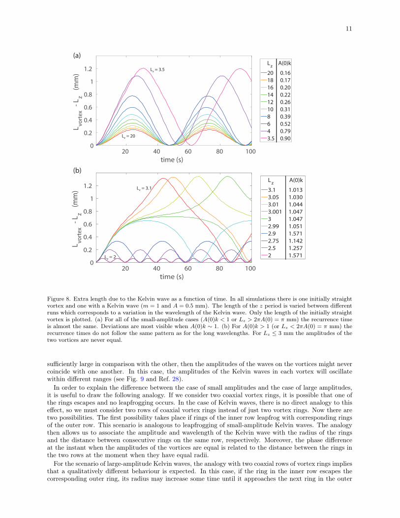
In the preceding sections we have focused on small-amplitude Kelvin waves and derived a model toexplain the observed recurrence phenomena in this limit. We will now consider what happens if we relaxthe assumption of small-amplitude Kelvin waves. The model we have derived is no longer applicable in thisparameter regime and we will proceed by relying on numerical simulations alone. To identify qualitativedifferences in the dynamics of the vortices, we have tracked how the length of one of the vortices in oursimulations changes with time (see Fig. 8). This provides sufficient insight into the dynamics because, for ahelix, the amplitude and length are related through the expression Lhelix = Lz

√1 + (Ak)2. The amplitude

of the other vortex can then be recovered by using momentum conservation. The results of our simulations,presented in Fig. 8, reveal that if the amplitude is increased, the frequency of the recurrence is modified,indicating that the vortex motion is being influenced by nonlinear effects. Moreover, for sufficiently largeamplitudes, there is a qualitative change in the behaviour of the system, indicating a transition from onetype of recurrent motion to another. In addition, if the Kelvin wave amplitude of one of the vortices is

11

time (s)20 40 60 80 100

L vort

ex -

L z (m

m)

0

0.2

0.4

0.6

0.8

1

1.2Lz A(0)k

20 0.1618 0.1716 0.2014 0.2212 0.2610 0.318 0.396 0.524 0.793.5 0.90

Lz = 3.5

Lz = 20

time (s)20 40 60 80 100

L vort

ex -

L z (m

m)

0

0.2

0.4

0.6

0.8

1

1.2Lz A(0)k

3.1 1.0133.05 1.0303.01 1.0443.001 1.0473 1.0472.99 1.0512.9 1.5712.75 1.1422.5 1.2572 1.571Lz = 2

Lz = 3.1

(a)

(b)

Figure 8. Extra length due to the Kelvin wave as a function of time. In all simulations there is one initially straightvortex and one with a Kelvin wave (m = 1 and A = 0.5 mm). The length of the z period is varied between differentruns which corresponds to a variation in the wavelength of the Kelvin wave. Only the length of the initially straightvortex is plotted. (a) For all of the small-amplitude cases (A(0)k < 1 or Lz > 2πA(0) = π mm) the recurrence timeis almost the same. Deviations are most visible when A(0)k ∼ 1. (b) For A(0)k > 1 (or Lz < 2πA(0) = π mm) therecurrence times do not follow the same pattern as for the long wavelengths. For Lz ≤ 3 mm the amplitudes of thetwo vortices are never equal.

sufficiently large in comparison with the other, then the amplitudes of the waves on the vortices might nevercoincide with one another. In this case, the amplitudes of the Kelvin waves in each vortex will oscillatewithin different ranges (see Fig. 9 and Ref. 28).

In order to explain the difference between the case of small amplitudes and the case of large amplitudes,it is useful to draw the following analogy. If we consider two coaxial vortex rings, it is possible that one ofthe rings escapes and no leapfrogging occurs. In the case of Kelvin waves, there is no direct analogy to thiseffect, so we must consider two rows of coaxial vortex rings instead of just two vortex rings. Now there aretwo possibilities. The first possibility takes place if rings of the inner row leapfrog with corresponding ringsof the outer row. This scenario is analogous to leapfrogging of small-amplitude Kelvin waves. The analogythen allows us to associate the amplitude and wavelength of the Kelvin wave with the radius of the ringsand the distance between consecutive rings on the same row, respectively. Moreover, the phase differenceat the instant when the amplitudes of the vortices are equal is related to the distance between the rings inthe two rows at the moment when they have equal radii.

For the scenario of large-amplitude Kelvin waves, the analogy with two coaxial rows of vortex rings impliesthat a qualitatively different behaviour is expected. In this case, if the ring in the inner row escapes thecorresponding outer ring, its radius may increase some time until it approaches the next ring in the outer

12

t (s)0 20 40 60 80 100

A (

mm

)

0

0.1

0.2

0.3

0.4

0.5

0.6

t (s)0 50 100

∆φ

0

π

2π

Figure 9. Amplitudes and phase difference (inset) as a function of time. Initially, one of the vortices is straight andthe other vortex has a Kelvin wave (m = 1, A = 0.5 mm, and Lz = 2.5 mm). In the large-amplitude regime, theamplitudes oscillate within different ranges.

row. Then the inner ring shrinks and passes through the outer ring and this cycle repeats. This analogy canprovide a qualitative interpretation for the change in leapfrogging of Kelvin waves between small amplitudesand large amplitudes. Furthermore, it provides an explanation for the sudden qualitative difference in therecurrence phenomena as the amplitudes are increased. However, care must be taken not to push this analogytoo far as it cannot provide accurate quantitative predictions. In particular, rings having amplitudes anddistances that are similar to Kelvin wave amplitudes and wavelengths will not behave in exactly the sameway.

VI. CONCLUSIONS

We have shown that coaxial vortices with the same Kelvin wave mode exchange energy in a periodicfashion. The helical vortices move through each other in a way that is similar to leapfrogging vortex rings.In the small-amplitude limit, the amplitudes of the two helical waves oscillate within the same range. Incontrast, in the large-amplitude limit, the amplitudes oscillate around two different mean values, althoughleapfrogging continues to occur in a periodic fashion.

Using a simplified model for nearly parallel vortices, we were able to explain the leapfrogging behaviourobserved in our Biot-Savart simulations in the limit of small-amplitude Kelvin waves. The success of themodel in this regime suggests that it may be possible to generalize it to other contexts, most notably instudying how adjacent vortex filaments can influence the theoretically predicted Kelvin wave cascades inthe high-wave-number regime of superfluid turbulence. For example, such a scenario would be relevant tounderstanding Kelvin waves on polarized vortex bundles that are believed to form in superfluid turbulence.

In the large-amplitude Kelvin wave regime, there is a qualitative change in the dynamical behaviour ofthe vortices. We have been able to interpret this by drawing an analogy with the dynamics of coaxial rows ofvortex rings. We end by noting that the phenomena predicted here will also contribute to our understandingof the dynamics of vortices and their interaction in classical fluids.

ACKNOWLEDGMENTS

R.H. and N.H. acknowledge financial support from the Academy of Finland. H.S. acknowledges supportfor a Research Fellowship from the Leverhulme Trust under Grant R201540. N.H. thanks CSC – IT Centerfor Science, Finland, for computational resources.

13

REFERENCES

1H. Helmholtz, Über Integrale der hydrodynamischen Gleichungen welche denWirbelbewegungen entsprechen, J. Reine Angew.Math. 55, 25 (1858).

2V. V. Meleshko, Coaxial axisymmet ric vortex rings: 150 years after Helmholtz, Theor. Comput. Fluid Dyn. 24, 403 (2010).3F. W. Dyson, The Potential of an Anchor Ring. Part II, Phil. Trans. R. Soc. Lond. A 184, 1041 (1893).4W. M. Hicks, On the Mutual Threading of Vortex Rings, Proc. R. Soc. Lond. Ser. A 102, 111 (1922).5A. V. Borisov, A. A. Kilin, and I. S. Mamaev, The dynamics of vortex rings: Leapfrogging, choreographies and the stabilityproblem, Regul. Chaotic Dyn. 18, 33 (2013).

6D. H. Wacks, A. W. Baggaley, and C. F. Barenghi, Coherent laminar and turbulent motion of toroidal vortex bundles, Phys.Fluids 26, 027102 (2014).

7R. M. Caplan, J. D. Talley, R. Carretero-González, and P. G. Kevrekidis, Scattering and leapfrogging of vortex rings in asuperfluid, Phys. Fluids 26, 097101 (2014).

8W. F. Vinen, Decay of superfluid turbulence at a very low temperature: The radiation of sound from a Kelvin wave on aquantized vortex, Phys. Rev. B 64, 134520 (2001).

9E. Kozik and B. Svistunov, Theory of Decay of Superfluid Turbulence in the Low-Temperature Limit, J. Low Temp. Phys.156, 215 (2009).

10L. Boué, R. Dasgupta, J. Laurie, V. L’vov, S. Nazarenko, and I. Procaccia, Exact solution for the energy spectrum ofKelvin-wave turbulence in superfluids, Phys. Rev. B 84, 064516 (2011).

11R. J. Donnelly, Quantized vortices in helium II, (Cambridge University Press, Cambridge, 1991).12C. F. Barenghi, M. Tsubota, A. Mitani, and T. Araki, Transient growth of Kelvin waves on quantized vortices, J. Low Temp.Phys. 134, 489 (2004).

13R. Jain and A. T. Conlisk, Interaction of Tip-Vortices in the Wake of a Two-Bladed Rotor in Axial Flight, J. Am. HelicopterSoc. 45, 157 (2000).

14J. Stack, F. X. Caradonna, and Ö. Savaş, Flow Visualizations and Extended Thrust Time Histories of Rotor Vortex Wakesin Descent, J. Am. Helicopter Soc. 50 279 (2005).

15V. L. Okulov and J. N. Sørensen, Stability of helical tip vortices in a rotor far wake, J. Fluid Mech. 576, 1 (2007).16S. Ivanell, R. Mikkelsen, J. N. Sørensen, and D. Henningson, Stability analysis of the tip vortices of a wind turbine, WindEnerg. 13, 705 (2010).

17M. Felli, R. Camussi, and F. Di Felice, Mechanisms of evolution of the propeller wake in the transition and far fields, J. FluidMech. 682, 5 (2011).

18S. Sarmast, R. Dadfar, R. F. Mikkelsen, P. Schlatter, S. Ivanell, J. N. Sørensen, and D. S. Henningson, Mutual inductanceinstability of the tip vortices behind a wind turbine, J. Fluid Mech. 755, 705 (2014).

19T. Leweke, H. U. Quaranta, H. Bolnot, F. J. Blanco-Rodríguez, and S. Le Dizès, Long- and short-wave instabilities in helicalvortices, J. Phys.: Conf. Ser. 524, 012154 (2014).

20I. Delbende, B. Piton, and M. Rossi, Merging of two helical vortices, Eur. J. Mech. B-Fluid 49, 363 (2015).21A. Nemes, D. L. Jacono, H. M. Blackburn, and J. Sheridan, Mutual inductance of two helical vortices, J. Fluid Mech. 774,298 (2015).

22C. Selçuk, Numerical study of helical vortices and their instabilities, Ph.D. thesis, Université Pierre et Marie Curie, 2016.23K. W. Schwarz, Three-dimensional vortex dynamics in superfluid 4He: Line-line and line-boundary interactions, Phys. Rev.B 31, 5782 (1985).

24R. I. Epstein and G. Baym, Vortex drag and the spin-up time scale for pulsar glitches, Astrophys. J. 387, 276 (1991).25H. Hasimoto, A soliton on a vortex filament, J. Fluid Mech. 51, 477 (1972).26E. B. Sonin, Dynamics of helical vortices and helical-vortex rings, Europhys. Lett. 97, 46002 (2012).27N. Hietala and R. Hänninen, Comment on “Motion of a helical vortex filament in superfluid 4He under the extrinsic form ofthe local induction approximation” [Phys. Fluids 25, 085101 (2013)], Phys. Fluids 26, 019101 (2014).

28See Supplemental Material at publishers web page for animations of leapfrogging Kelvin waves.29R. Klein, A. J. Majda, and K. Damodaran, Simplified equations for the interactions of nearly parallel vortex filaments, J.Fluid Mech. 288, 201 (1995).

30V. E. Zakharov, Quasi-Two-Dimensional Hydrodynamics and Interaction of Vortex Tubes, in Nonlinear MHD Waves andTurbulence: Proceeding of the Workshop Held in Nice, France, 1–4 December 1998 edited by T. Passot and P.-L. Sulem(Springer, Berlin, 1999).