institute of aeronautical engineering · 2019-08-07 · source from modern compressible flow with...
TRANSCRIPT

IARE High Speed Aerodynamics P a g e | 1
Source from Modern Compressible flow with historical perspective by John D. Anderson
INSTITUTE OF AERONAUTICAL ENGINEERING (Autonomous)
Dundigal, Hyderabad -500 043
AERONAUTICAL ENGINEERING
COURSE LECTURE NOTES
Course Name HIGH SPEED AERODYNAMICS
Course Code AAE008
Programme B.Tech
Semester V
Course Coordinator Mr. G. Staya Dileep, Assistant Professor, AE
Course Faculty Mr. G. Staya Dileep, Assistant Professor, AE
Ms D. Anitha, Assistant Professor, AE
Lecture Numbers 1-60
Topic Covered All
COURSE OBJECTIVES (COs):
The course should enable the students to:
I Understand the effect of compressibility at high-speeds and the ability to make intelligent design
decisions.
II Explain the dynamics in subsonic, transonic and supersonic flow regimes in both internal and
external geometries.
III Analyze the airfoils at subsonic, transonic and supersonic flight conditions using the perturbed flow
theory assumption.
IV Formulate appropriate aerodynamic models to predict the forces and performance of realistic three
dimensional configurations.
COURSE LEARNING OUTCOMES (CLOs):
Students, who complete the course, will have demonstrated the ability to do the following:
S. No Description
AAE008.01 Demonstrate the concept of supersonic flow, how it is different from incompressible flow.
AAE008.02 Understand governing equations of supersonic flow in various form and thermodynamics
properties.
AAE008.03 Describe the governing equations required for compressible flows.
AAE008.04 Illustrate the impact of supersonic flow in the presence of compression and expansion corner
AAE008.05 Demonstrate supersonic aircraft design and applications to aircrafts, supersonic wind tunnel,
shock tubes.
AAE008.06 Understand the concepts of shock wave boundary layer interaction.
IARE High Speed Aerodynamics P a g e | 2
Source from Modern Compressible flow with historical perspective by John D. Anderson
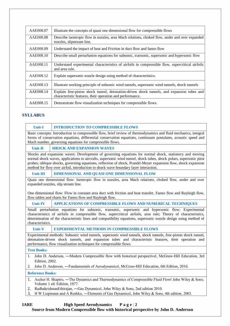
AAE008.07 Illustrate the concepts of quasi one dimensional flow for compressible flows
AAE008.08 Describe isentropic flow in nozzles, area Mach relations, choked flow, under and over expanded
nozzles, slipstream line.
AAE008.09 Understand the impact of heat and Friction in duct flow and fanno flow
AAE008.10 Describe small perturbation equations for subsonic, transonic, supersonic and hypersonic flow
AAE008.11 Understand experimental characteristics of airfoils in compressible flow, supercritical airfoils
and area rule.
AAE008.12 Explain supersonic nozzle design using method of characteristics.
AAE008.13 Illustrate working principle of subsonic wind tunnels, supersonic wind tunnels, shock tunnels
AAE008.14 Explain free-piston shock tunnel, detonation-driven shock tunnels, and expansion tubes and characteristic features, their operation and performance.
AAE008.15 Demonstrate flow visualization techniques for compressible flows.
SYLLABUS
Unit-I INTRODUCTION TO COMPRESSIBLE FLOWS
Basic concepts: Introduction to compressible flow, brief review of thermodynamics and fluid mechanics, integral
forms of conservation equations, differential conservation equations, continuum postulates, acoustic speed and
Mach number, governing equations for compressible flows.
Unit-II SHOCK AND EXPANSION WAVES
Shocks and expansion waves: Development of governing equations for normal shock, stationery and moving
normal shock waves, applications to aircrafts, supersonic wind tunnel, shock tubes, shock polars, supersonic pitot
probes; oblique shocks, governing equations, reflection of shock, Prandtl-Meyer expansion flow, shock expansion
method for flow over airfoil, introduction to shock wave boundary layer interaction.
Unit-III DIMENSIONAL AND QUASI ONE DIMENSIONAL FLOW
Quasi one dimensional flow: Isentropic flow in nozzles, area Mach relations, choked flow, under and over
expanded nozzles, slip stream line.
One dimensional flow: Flow in constant area duct with friction and heat transfer, Fanno flow and Rayleigh flow,
flow tables and charts for Fanno flow and Rayleigh flow.
Unit-IV APPLICATIONS OF COMPRESSIBLE FLOWS AND NUMERICAL TECHNIQUES
Small perturbation equations for subsonic, transonic, supersonic and hypersonic flow; Experimental
characteristics of airfoils in compressible flow, supercritical airfoils, area rule; Theory of characteristics,
determination of the characteristic lines and compatibility equations, supersonic nozzle design using method of characteristics.
Unit-V EXPERIMENTAL METHODS IN COMPRESSIBLE FLOWS
Experimental methods: Subsonic wind tunnels, supersonic wind tunnels, shock tunnels, free-piston shock tunnel,
detonation-driven shock tunnels, and expansion tubes and characteristic features, their operation and
performance, flow visualization techniques for compressible flows
Text Books:
1. John D. Anderson, ―Modern Compressible flow with historical perspective‖, McGraw-Hill Education, 3rd
Edition, 2002.
2. John D. Anderson, ―Fundamentals of Aerodynamics‖, McGraw-Hill Education, 6th Edition, 2016.
Reference Books:
1. Ascher H. Shapiro, ―The Dynamics and Thermodynamics of Compressible Fluid Flow‖ John Wiley & Sons; Volume 1 ed. Edition, 1977.
2. RadhakrishnanEthirajan, ―Gas Dynamics‖, John Wiley & Sons, 2nd edition 2010.
3. H W Liepmann and A Roshko, ―Elements of Gas Dynamics‖, John Wiley & Sons, 4th edition, 2003.

IARE High Speed Aerodynamics P a g e | 3
Source from Modern Compressible flow with historical perspective by John D. Anderson
UNIT - I
INTRODUCTION TO COMPRESSIBLE FLOW
1.1 Introduction
Compressible flow is often called as variable density flow. For the flow of all liquids and for the flow of
gases under certain conditions, the density changes are so small that assumption of constant density
remains valid.Let us consider a small element of fluid of volume. The pressure exerted on the element by
the neighboring fluid is p. If the pressure is now increased by an amount dp, the volume of the element
will correspondingly be reduced by the amount d .The compressibility of the fluid K is thus defined as
𝑲 =𝟏
𝝆.𝒅𝝆
𝒅𝒑
However, when a gas is compressed, its temperature increases. Therefore, the above mentioned definition
of compressibility is not complete unless temperature condition is specified. When the temperature is
maintained at a constant level, the isothermal compressibility is defined as
𝐾𝜏 = − 1
⩝(
𝑑 ⩝
𝑑𝑃)
𝜏
Compressibility is a property of fluids. Liquids have very low value of compressibility (for ex.
compressibility of water is 5 × 10⁻¹⁰ m2/N at 1 atm under isothermal condition), while gases have very
high compressibility (for ex. compressibility of air is 10-5 m2/N at 1 atm under isothermal condition).
Categories of flow for external aerodynamics
Ma < 0.3: incompressible flow; change in density is negligible.
0.3< Ma < 0.8: subsonic flow; density changes are significant but shock waves do not appear.
0.8< Ma < 1.2: transonic flow; shock waves appear and divide the subsonic and supersonic regions
of the flow. Transonic flow is characterized by mixed regions of locally subsonic
and supersonic flow
1.2 < Ma < 3.0: supersonic flow; flow field everywhere is above acoustic speed. Shock waves
appear and across the shock wave, the streamline changes direction
discontinuously.
3.0<Ma: hypersonic flow; where the temperature, pressure and density of the flow increase almost
explosively across the shock wave.
1.2 Brief Review of Thermodynamics and Fluid Mechanics
1.2.1 Thermodynamics Concepts:
1.2.1.1 System
A thermodynamic system is defined as a definite quantity of matter or a region in space upon which
attention is focused in the analysis of a problem. We may want to study a quantity of matter contained
with in a closed rigid walled chambers, or we may want to consider something such as gas pipeline
through which the matter flows. The composition of the matter inside the system may be fixed or may
change through chemical and nuclear reactions. A system may be arbitrarily defined. It becomes

IARE High Speed Aerodynamics P a g e | 4
Source from Modern Compressible flow with historical perspective by John D. Anderson
important when exchange of energy between the system and the everything else outside the system is
considered. The judgment on the energetics of this exchange is very important.
1.2.1.2 Surroundings
Everything external to the system is surroundings. The system is distinguished from its surroundings by a
specified boundary which may be at rest or in motion. The interactions between a system and its
surroundings, which take place across the boundary, play an important role in thermodynamics. A system
and its surroundings together comprise a universe.
1.2.1.3 Types of systems
Two types of systems can be distinguished. These are referred to, respectively, as closed systems and
open systems or control volumes. A closed system or a control mass refers to a fixed quantity of matter,
whereas a control volume is a region in space through which mass may flow. A special type of closed
system that does not interact with its surroundings is called an Isolated system.
Two types of exchange can occur between the system and its surroundings:
1. energy exchange (heat or work)and
2. Exchange of matter (movement of molecules across the boundary of the system and
surroundings).
Based on the types of exchange, one can define
isolated systems: no exchange of matter andenergy
closed systems: no exchange of matter but some exchange ofenergy
open systems: exchange of both matter andenergy
If the boundary does not allow heat (energy) exchange to take place it is called adiabatic boundary
otherwise it is diathermalboundary.
1.2.2 Laws of thermodynamics
1.2.2.1 Zeroth law of thermodynamics: This law states that ‘when system A is in thermal equilibrium
with system B and system B is separately in thermal equilibrium with system C then system A and C are
also in thermalequilibrium’.
This law portrays temperature as a property of the system and gives basis of temperature measurement.
1.2.2.2 First law of thermodynamics: It states the energy conservation principle, ‘energy can neither be
created nor be destroyed but one form of the energy can be converted toother’.
Implementationof first law for a thermodynamic process defines ‘internal energy’ as a property of the
system. According to this law for a closed system, when some amount of heat is supplied to the system,
part of it is used to convert into work and rest is stored in the system in the form of internal energy. For the
open system, heat supplied splits into enthalpy change and work done by the system.
First law of thermodynamics is thus associated with a corollary which states that there can be no machine
(Perpetual Motion Machine of first kind) which can produce continuous work output without having any
heat interaction with the surrounding.
1.2.2.3 Second law of thermodynamics: There are two statements of second law of thermodynamics.
1.2.2.4 Clausius statement: It is impossible to construct a system which will operate in a cycle, transfers
heat from the low temperature reservoir (or object) to the high temperature reservoir (or object) without
any external effect or work interaction with surrounding.
1.2.2.5 Kelvin Plank statement: It is impossible to construct a heat engine which produces work in a
cycle while interacting with only one reservoir.

IARE High Speed Aerodynamics P a g e | 5
Source from Modern Compressible flow with historical perspective by John D. Anderson
Kelvin Plank statement necessarily states that Perpetual Motion Machine of second kind is impossible.
These statements introduce a new property termed as entropy which is the measure of disorder.
There are some corollaries of second law of thermodynamics
1. All the reversible heat engines working between same temperature limits have same efficiency.
2. Irreversible heat engine working in the same temperature limit as the reversible heat engine will
have lower efficiency.
The second law of thermodynamics leads to an inequality called as Clausius inequality which is valid for
general process happening in any system. This law grades the energies according to which work is high
grade energy and heat is low grade energy. Therefore second law of thermodynamics directs that low
grade energy can not be completely converted into high grade energy. This law also states the possibility
of having a process in reality unlike the first law which can at most quantify the effects of the process if
process becomes a reality. Hence according to second law only those processes are possible in which
entropy of the universe increase or at least remain constant. This is called as entropy increase principle
which also states that entropy of an isolated system always increases or remains constant.
1.2.2.6 Third law of thermodynamics: ‘Entropy of pure substance in thermodynamic equilibrium is zero
at absolute zero temperature’. Therefore according to this law, there exists zero Kelvin temperature on the
temperature scale but it is difficult to achieve the same.
1.2.2.7 Isentropic relations:
Isentropic relations are the relations between thermodynamic properties if the system undergoes
isentropic process.
Consider a closed system interacting dQ amount of energy with the surrounding. If dU is the change in
internal energy of the system and pdV is work done by the system against pressure p due to volume
change dV. According to First Law of Thermodynamics we know that,
dQ = dU + pdV
From Second law of Thermodynamics,
𝑑𝑄
𝑇= 𝑑𝑆
dQ = TdS
Here dS is the entropy change due to reversible heat interaction dQ.
Therefore, combining First and Second Laws of Thermodynamics,
TdS = dU + pdV
However, we know that, if H is enthalpy of the system then,
H = U + pV
dH = dU + pdV + VdP
dH - Vdp = dU + pdV
Combining equations we get,
TdS = dH – Vdp
For system with unit mass of matter, above equation can be written as,
Tds = dh - vdp
For the special case, if system undergoes reversible adiabatic or isentropic process then, entropy change
of the system (dS ) is zero.

IARE High Speed Aerodynamics P a g e | 6
Source from Modern Compressible flow with historical perspective by John D. Anderson
CpdT = vdp
From ideal gas relation, v = RT/P, above equations becomes
𝐶𝑃𝑑𝑇 =𝑅𝑇
𝑃𝑑𝑝
𝐶𝑃𝑑𝑇
𝑅𝑇=
𝑑𝑝
𝑃
We know the relations between specific heats as
𝐶𝑃 − 𝐶𝑣 = 𝑅
𝐶𝑃 −𝐶𝑃
𝛾= 𝑅
𝐶𝑃 =ϒ𝑅
𝛾 − 1
𝐶𝑣 =𝑅
𝛾 − 1
Substituting above expression for Cp in equation (1.4), we get
𝛾
𝛾 − 1
𝑑𝑇
𝑇=
𝑑𝑝
𝑃
Integrating above equation from state 1 to state 2 for the isentropic process of the system, we get,
𝛾
𝛾 − 1𝑙𝑛 (
𝑇2
𝑇1) = ln (
𝑃2
𝑃1)
(𝑃2
𝑃1) = (
𝑇2
𝑇1)
𝛾
𝛾−1
Since the system is undergoing adiabatic process from state 1 to state 2,
𝑃
𝜌𝛾= 𝑐𝑜𝑛𝑠𝑡
(𝜌1
𝜌2) = (
𝑇2
𝑇1)
1
𝛾−1
Here relations are called as isentropic equations.

IARE High Speed Aerodynamics P a g e | 7
Source from Modern Compressible flow with historical perspective by John D. Anderson
1.3 Important Fluid Properties
1.3.1 Continuum:
Fluid matter is made up of molecules or atoms. However for most of the fluid dynamic calculations
discrete presence of these elementary objects is neglected and fluid matter is assumed to be continuous
for prediction of various fluid flow phenomenon or for measurement of fluid properties. If a pressure
probe concentrates to a very small area, of molecular dimensions, in the fluid flow, then fluctuations can
be observed in the measurements due to random presence of molecules. Therefore any measurement
probe used for experiments or fluid property estimation should not have very small probe area in order to
incur molecular fluctuations. If average number of molecules colliding the probing area over the time is
very large then these fluctuations die out and we get a constant macroscopic value of the property. For
these conditions we can comfortably make the assumptions of continuum of matter.
Continuous presence of the matter is called as continuum. This is the assumption which we will be using
for most of the derivations of this course. This assumption helps us for calculation of gradient and flow
variables smoothly. The governing non-dimensional parameter for prediction of continuum is Knudsen
number which is defined as the ratio of mean free path to the characteristic length of the object. Here
mean free path should be understood as the mean distance traveled by a molecule between two successive
collisions with other molecules. Thus calculated Knudsen number should be close to zero or below 0.3 for
use of most of the relations or governing equations. Mean free path of standard atmosphere is 5 x 10⁻⁸ m
due to very high density of air near the earth’s surface. Therefore Knudsen number remains close to zero
for general fluid dynamic situations. Validation of continuum assumption and in turn the usage of
governing equations in their standard form remain intact till the altitude of around 90 km from earth
surface where Knudsen number is below 0.3.
Above the first critical value of Knudsen number (0.3), usefulness of governing equations in their
standard form is intact however the nature of boundary conditions changes due to existence of velocity
and temperature slip on the wall. From 90 Km till 150 km from earth surface, density becomes low as a
effect of which fluid velocity and temperature at the surface do not remain in equilibrium with the
surface. Therefore for the Knudsen number range 0.3 to 1, which is also called as transitional regime, slip
wall boundary conditions should be used along with the usual governing equations based on continuum
assumption
Presence of free molecular flow can be assured If Knudsen number crosses 1. Kinetic theory of gases and
related equations are generally prescribed if the Knudsen number crosses its second critical value. This
conditions persists beyond,150 km from earth’s surface where density of air is very low.
1.3.2 Transport phenomenon:
Diffusion of mass, momentum and heat always take place from the region of higher concentration to the
region of lower concentration.
Concentration gradient of mass leads to mass transfer. Fick's law gives the quantification of mass
transport through the linear relation between massflux and gradient of concentration. The proportionality
constant (mass diffusion coefficient) depends on gases involved in the diffusion and their thermodynamic
state. According to this law, diffusion of nitrogen in oxygen is different from diffusion of nitrogen in
methane. Diffusion of nitrogen in oxygen also depends on pressure and temperature conditions. Sainted
stick is the example of concentration based mass diffusion.

IARE High Speed Aerodynamics P a g e | 8
Source from Modern Compressible flow with historical perspective by John D. Anderson
Temperature variation leads to heat transfer. Fourier's law gives the relation between heatflux and
gradient for temperature. The proportionality constant is the material property (thermal conductivity) and
depends mainly on temperature of the material. Heat transfer taking place in boiler walls, fins etc are the
examples of conduction heat transfer.
Newton's law of momentum diffusion states that momentum flux is proportional to the gradient of
velocity. The proportionality constant of this relation is the fluid property (viscosity) which depends
mainly on temperature of the fluid. Presence of boundary layer near the wall, in case of fluid flow over
the same, is the example of momentum diffusion.
Transport equations have flux equated with gradient where only first derivatives appear in gradient terms.
The reason behind this is that, diffusion is the microscopic phenomenon hence it does not account for
curvature involved with higher derivatives. Along with this there is no higher power term in this equation
since these equations are valid for small concentration gradients but it has been seen that these equations
hold good for higher concentrations also.
1.3.3. Compressibility of fluid and flow:
If application of pressure changes volume or density of the fluid then fluid is said to be compressible.
𝑐𝑜𝑚𝑝𝑟𝑒𝑠𝑠𝑖𝑏𝑖𝑙𝑖𝑡𝑦(𝜏) = −1
𝜗
𝜕𝜗
𝜕𝑃=
1
𝜌
𝜕𝜌
𝜕𝑃
Compressibility is thus inverse of bulk modulus. Hence compressibility can be defined as the incurred
volumetric strain for unit change in pressure. Negative sign in the above expression is the fact that
volume decreases with increase in applied pressure. For example, air is more compressible than water.
Since definition of compressibility involves change in volume due to change in pressure, hence
compressibility can be isothermal, where volume change takes place at constant temperature or isentropic
where volume change takes place at constant entropy.
𝐼𝑠𝑜𝑡ℎ𝑒𝑟𝑚𝑎𝑙 𝑐𝑜𝑚𝑝𝑟𝑒𝑠𝑠𝑖𝑏𝑖𝑙𝑖𝑡𝑦(𝜏) = −1
𝜗(
𝜕𝜗
𝜕𝑃)
𝜏=𝑐𝑜𝑛𝑠𝑡𝑎𝑛𝑡=
1
𝜌(
𝜕𝜌
𝜕𝑃)
𝜏=𝑐𝑜𝑛𝑠𝑡𝑎𝑛𝑡
𝐼𝑠𝑒𝑛𝑡𝑟𝑜𝑝𝑖𝑐 𝑐𝑜𝑚𝑝𝑟𝑒𝑠𝑠𝑖𝑏𝑖𝑙𝑖𝑡𝑦(𝜏) = −1
𝜗(
𝜕𝜗
𝜕𝑃)
𝑠=𝑐𝑜𝑛𝑠𝑡𝑎𝑛𝑡=
1
𝜌(
𝜕𝜌
𝜕𝑃)
𝑠=𝑐𝑜𝑛𝑠𝑡𝑎𝑛𝑡
Also, for isothermal compressibility we know,
𝜏 = −1
𝜗(
𝜕𝜗
𝜕𝑃)
𝜏=𝑐𝑜𝑛𝑠𝑡𝑎𝑛𝑡
Since P𝜗 = 𝑅𝑇 for ideal gas, we have,
(𝜕𝜗
𝜕𝑃)
𝜏=𝑐𝑜𝑛𝑠𝑡𝑎𝑛𝑡= −
𝜗
𝑃
Hence, isothermal compressibility is
τ=1/ρ
For isentropic compressibility we know,
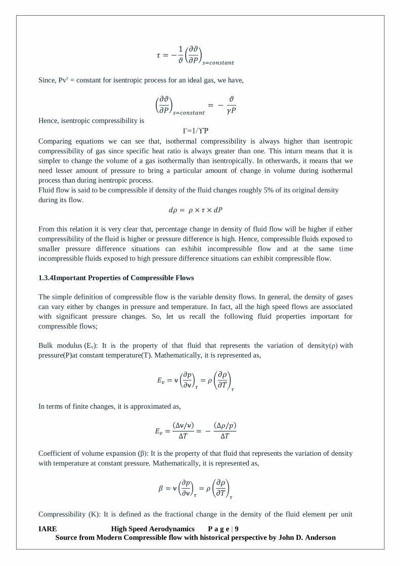
IARE High Speed Aerodynamics P a g e | 9
Source from Modern Compressible flow with historical perspective by John D. Anderson
𝜏 = −1
𝜗(
𝜕𝜗
𝜕𝑃)
𝑠=𝑐𝑜𝑛𝑠𝑡𝑎𝑛𝑡
Since, Pvγ = constant for isentropic process for an ideal gas, we have,
(𝜕𝜗
𝜕𝑃)
𝑠=𝑐𝑜𝑛𝑠𝑡𝑎𝑛𝑡= −
𝜗
𝛾𝑃
Hence, isentropic compressibility is
Γ=1/ϒP
Comparing equations we can see that, isothermal compressibility is always higher than isentropic
compressibility of gas since specific heat ratio is always greater than one. This inturn means that it is
simpler to change the volume of a gas isothermally than isentropically. In otherwards, it means that we
need lesser amount of pressure to bring a particular amount of change in volume during isothermal
process than during isentropic process.
Fluid flow is said to be compressible if density of the fluid changes roughly 5% of its original density
during its flow.
𝑑𝜌 = 𝜌 × 𝜏 × 𝑑𝑃
From this relation it is very clear that, percentage change in density of fluid flow will be higher if either
compressibility of the fluid is higher or pressure difference is high. Hence, compressible fluids exposed to
smaller pressure difference situations can exhibit incompressible flow and at the same time
incompressible fluids exposed to high pressure difference situations can exhibit compressible flow.
1.3.4Important Properties of Compressible Flows
The simple definition of compressible flow is the variable density flows. In general, the density of gases
can vary either by changes in pressure and temperature. In fact, all the high speed flows are associated
with significant pressure changes. So, let us recall the following fluid properties important for
compressible flows;
Bulk modulus (Ev): It is the property of that fluid that represents the variation of density(ρ) with
pressure(P)at constant temperature(T). Mathematically, it is represented as,
𝐸𝑣 = v (𝜕𝑝
𝜕v)
𝜏= 𝜌 (
𝜕𝜌
𝜕𝑇)
𝜏
In terms of finite changes, it is approximated as,
𝐸𝑣 =(∆v/v)
∆𝑇= −
(∆𝜌/𝑝)
∆𝑇
Coefficient of volume expansion (β): It is the property of that fluid that represents the variation of density
with temperature at constant pressure. Mathematically, it is represented as,
𝛽 = v (𝜕𝑝
𝜕v)
𝜏= 𝜌 (
𝜕𝜌
𝜕𝑇)
𝜏
Compressibility (K): It is defined as the fractional change in the density of the fluid element per unit

IARE High Speed Aerodynamics P a g e | 10
Source from Modern Compressible flow with historical perspective by John D. Anderson
change in pressure. One can write the expression for Kas follows;
𝑲 =𝟏
𝝆.𝒅𝝆
𝒅𝒑 𝐝𝛒 = 𝛒 𝐊 𝐝𝐩
In order to be more precise, the compression process for a gas involves increase in temperature depending
on the amount of heat added or taken away from the gas. If the temperature of the gas remains constant,
the definition is refined as isothermal compressibility (KT). On the other hand, when no heat is
added/taken away from the gases and in the absence of any dissipative mechanisms, the compression
takes place isentropically. It is then, called as isentropic compressibility(Ks).
𝐾𝑇 = 1
𝜌(
𝜕𝜌
𝜕𝑝)
𝑇
, 𝐾𝑠 = 1
𝜌(
𝜕𝜌
𝜕𝑝)
𝑠
1.3.5 Viscosity (μ):
Viscosity is a fluid property whose effect is understood when the fluid is in motion.
In a flow of fluid, when the fluid elements move with different velocities, each element will feel
some resistance due to fluid friction within the elements.
Therefore, shear stresses can be identified between the fluid elements with different velocities.
The relationship between the shear stress and the velocity field was given by Sir Isaac Newton.
Newton postulated that τ is proportional to the quantity Δu/ Δy where Δy is the distance of
separation of the two layers and Δu is the difference in their velocities.
In the limiting case of, Δu / Δy equals du/dy, the velocity gradient at a point in a direction
perpendicular to the direction of the motion of the layer.
According to Newton τ and du/dy bears the relation
𝜏 = 𝜇𝑑𝑢
𝑑𝑦
Where, the constant of proportionality μ is known as the coefficient of viscosity or simply viscosity which
is a property of the fluid and depends on its state. Sign of τ depends upon the sign of du/dy. For the
profile, du/dy is positive everywhere and hence,τ is positive. Both the velocity and stress are considered
positive in the positive direction of the coordinate parallel to them.
Equation
𝜏 = 𝜇𝑑𝑢
𝑑𝑦
defining the viscosity of a fluid, is known as Newton's law of viscosity. Common fluids, viz. water, air,
mercury obey Newton's law of viscosity and are known as Newtonian fluids.
Other classes of fluids, viz. paints, different polymer solution, blood do not obey the typical linear
relationship, of τ and du/dy and are known as non-Newtonian fluids.

IARE High Speed Aerodynamics P a g e | 11
Source from Modern Compressible flow with historical perspective by John D. Anderson
1.4 Integral forms of conservation equations
1.4.1 Conservation of Mass or Continuity Equation (Integral Form)
Consider the fluid domain. Our aim is to derive the mass conservation equation using this fluid domain of
arbitrary shape.
Fig.1.1 Finite Control Volume fixed in space
If there is no mass source in the control volume, we can equate the rate of change of mass inside the
control volume with the difference in influx and outflux of mass. Consider ρ as the density of the flow
which is function of space coordinates and time (ρ = ρ(x, y, z, t)). Let V be velocity vector of the flow
which is also function of space coordinates and time and has u, v and was three components aligned to the
coordinate axes x, y and z respectively. Consider elemental surface area (dS) of the control volume. This
area along with the unit normal.
Total mass inside the control volume can be found by summing the mass of elemental volumes
(dv) occupying the complete finite volume. We know that ρdυ is the mass of an elemental volume, hence
total mass inside the control volume can be written as
Total mass in the control volume (CV) = ∰ 𝜌𝑑𝑣
𝑣
Hence rate of change of this mass is,
Rate of change of mass in
CV=
𝜕
𝜕𝑡∰ 𝜌𝑑𝑣
𝑣
Thus the time rate of decrease of mass inside the
CV is
− 𝜕
𝜕𝑡∰ 𝜌𝑑𝑣
𝑣
The mass flow rate of any moving fluid across any fixed surface is equal to the product of density, area of
surface and component of velocity normal to the surface. Therefore, the elemental mass flow across the
area ds is expressed as
ρVndS = ρV.dS
Where Vn is the component of velocity normal to the surface. Thus the net mass flow out of the entire
volume through the control surface S is summation of mass flow rates through all elemental areas dS of
control surface S. Hence net flux through the control surface is
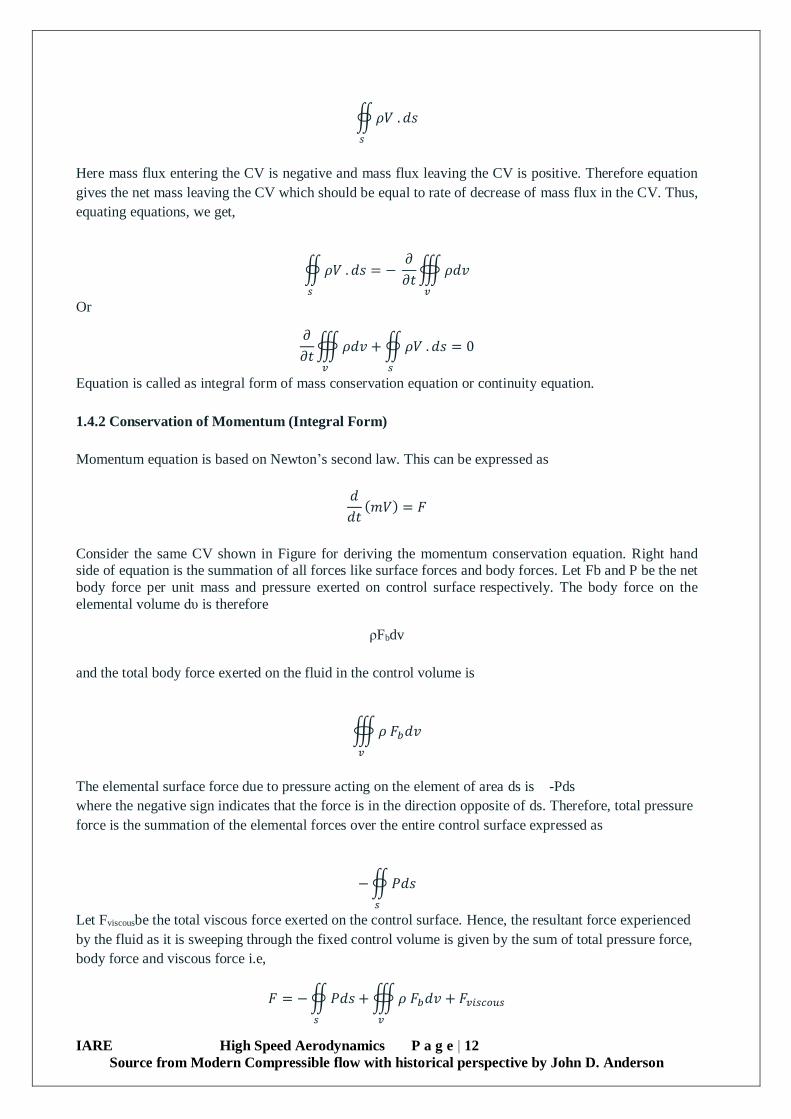
IARE High Speed Aerodynamics P a g e | 12
Source from Modern Compressible flow with historical perspective by John D. Anderson
∯ 𝜌𝑉 . 𝑑𝑠
𝑠
Here mass flux entering the CV is negative and mass flux leaving the CV is positive. Therefore equation
gives the net mass leaving the CV which should be equal to rate of decrease of mass flux in the CV. Thus,
equating equations, we get,
∯ 𝜌𝑉 . 𝑑𝑠
𝑠
= − 𝜕
𝜕𝑡∰ 𝜌𝑑𝑣
𝑣
Or
𝜕
𝜕𝑡∰ 𝜌𝑑𝑣
𝑣
+ ∯ 𝜌𝑉 . 𝑑𝑠
𝑠
= 0
Equation is called as integral form of mass conservation equation or continuity equation.
1.4.2 Conservation of Momentum (Integral Form)
Momentum equation is based on Newton’s second law. This can be expressed as
𝑑
𝑑𝑡(𝑚𝑉) = 𝐹
Consider the same CV shown in Figure for deriving the momentum conservation equation. Right hand side of equation is the summation of all forces like surface forces and body forces. Let Fb and P be the net
body force per unit mass and pressure exerted on control surface respectively. The body force on the
elemental volume dυ is therefore
ρFbdv
and the total body force exerted on the fluid in the control volume is
∰ 𝜌 𝐹𝑏𝑑𝑣
𝑣
The elemental surface force due to pressure acting on the element of area ds is -Pds
where the negative sign indicates that the force is in the direction opposite of ds. Therefore, total pressure
force is the summation of the elemental forces over the entire control surface expressed as
− ∯ 𝑃𝑑𝑠
𝑠
Let Fviscousbe the total viscous force exerted on the control surface. Hence, the resultant force experienced
by the fluid as it is sweeping through the fixed control volume is given by the sum of total pressure force,
body force and viscous force i.e,
𝐹 = − ∯ 𝑃𝑑𝑠
𝑠
+ ∰ 𝜌 𝐹𝑏𝑑𝑣
𝑣
+ 𝐹𝑣𝑖𝑠𝑐𝑜𝑢𝑠
IARE High Speed Aerodynamics P a g e | 13
Source from Modern Compressible flow with historical perspective by John D. Anderson
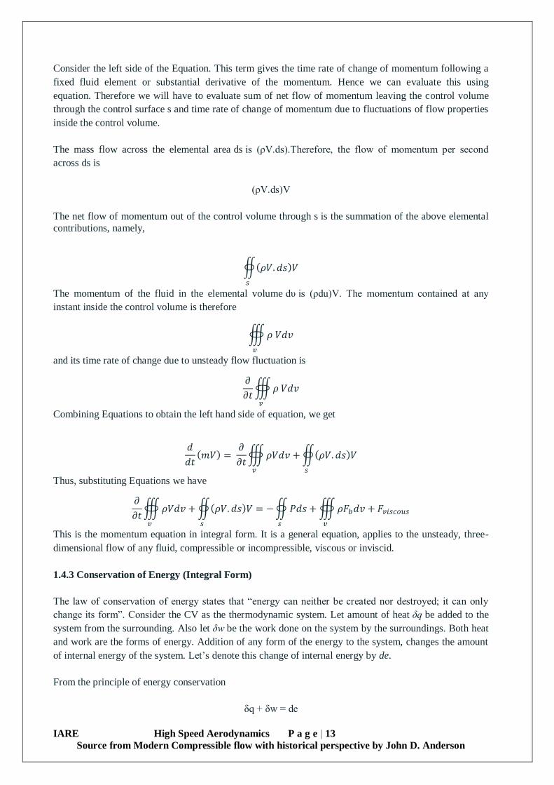
Consider the left side of the Equation. This term gives the time rate of change of momentum following a
fixed fluid element or substantial derivative of the momentum. Hence we can evaluate this using
equation. Therefore we will have to evaluate sum of net flow of momentum leaving the control volume
through the control surface s and time rate of change of momentum due to fluctuations of flow properties
inside the control volume.
The mass flow across the elemental area ds is (ρV.ds).Therefore, the flow of momentum per second
across ds is
(ρV.ds)V
The net flow of momentum out of the control volume through s is the summation of the above elemental
contributions, namely,
∯(𝜌𝑉. 𝑑𝑠)𝑉
𝑠
The momentum of the fluid in the elemental volume dυ is (ρdu)V. The momentum contained at any
instant inside the control volume is therefore
∰ 𝜌 𝑉𝑑𝑣
𝑣
and its time rate of change due to unsteady flow fluctuation is
𝜕
𝜕𝑡∰ 𝜌 𝑉𝑑𝑣
𝑣
Combining Equations to obtain the left hand side of equation, we get
𝑑
𝑑𝑡(𝑚𝑉) =
𝜕
𝜕𝑡∰ 𝜌𝑉𝑑𝑣
𝑣
+ ∯(𝜌𝑉. 𝑑𝑠)𝑉
𝑠
Thus, substituting Equations we have
𝜕
𝜕𝑡∰ 𝜌𝑉𝑑𝑣
𝑣
+ ∯(𝜌𝑉. 𝑑𝑠)𝑉
𝑠
= − ∯ 𝑃𝑑𝑠
𝑠
+ ∰ 𝜌𝐹𝑏𝑑𝑣
𝑣
+ 𝐹𝑣𝑖𝑠𝑐𝑜𝑢𝑠
This is the momentum equation in integral form. It is a general equation, applies to the unsteady, three-
dimensional flow of any fluid, compressible or incompressible, viscous or inviscid.
1.4.3 Conservation of Energy (Integral Form)
The law of conservation of energy states that “energy can neither be created nor destroyed; it can only
change its form”. Consider the CV as the thermodynamic system. Let amount of heat δq be added to the
system from the surrounding. Also let δw be the work done on the system by the surroundings. Both heat
and work are the forms of energy. Addition of any form of the energy to the system, changes the amount
of internal energy of the system. Let’s denote this change of internal energy by de.
From the principle of energy conservation
δq + δw = de

IARE High Speed Aerodynamics P a g e | 14
Source from Modern Compressible flow with historical perspective by John D. Anderson
Therefore in terms of rate of change the above equation changes to
𝛿𝑞
𝛿𝑡+
𝛿𝑤
𝛿𝑡=
𝛿𝑒
𝛿𝑡
If the system to be considered as a open system then the change will take place for all the forms of
energies owed by the system, like internal energy and kinetic energy. Hence right hand side of the above
equation is just the representation of change in energy content of the system.
Let’s first concentrate on first term on left hand side of above equation and evaluate the same. There are
various sources of heat addition in the system some of which are external heat addition from the
surrounding, heat addition by chemical energy release, heat addition by radiation etc. Let’s consider some
of those sources of heat addition and derive the energy equation. If q is the amount of heat added per unit
mass, then rate of heat addition for any elemental volume will be q(ρdv). Summing over the complete
control volume gives us total external volumetric heat addition. Heat might get added by viscous effects
like conduction. Hence net rate of heat addition can be,
𝛿𝑞
𝛿𝑡= ∰ 𝑞 𝜌 𝑑𝑣 + �̇�𝑣𝑖𝑠𝑐𝑜𝑢𝑠
𝑣
Consider the second term on left hand side of equation and evaluate the same. There are various ways by
which work transfer can be achieved to or from the system. Main source is the surface forces like
pressure, body force etc.
Considering the elemental area ds of the control surface. The pressure force on this elemental area is -
Pds and the rate of work done on the fluid passing through ds with velocity V is (-Pds).V. Hence,
summing over the complete control surface, rate of work done due to pressure force is,
− ∯(𝑃𝑑𝑠). 𝑉
𝑠
In addition, consider an elemental volume dυ inside the control volume. The rate of work done on the
elemental volume due to body force is (ρFbdu).V. Here Fb is the body force per unit mass. Summing over
the complete control volume, we obtain, rate of work done on fluid inside υ due to body forces is
∰(𝜌𝐹𝑏𝑑𝑣
𝑣
). 𝑉
If the flow is viscous, the shear stress on the control surface will also do work on the fluid as it passes
across the surface. Let Ẇviscous denote the work done due to the shear stress. Therefore, the total work
done on the fluid inside the control volume is the sum of terms and Ẇviscous that is
𝛿𝑤
𝛿𝑡= − ∯ 𝑃𝑉.
𝑠
𝑑𝑠 + ∰ 𝜌(𝐹𝑏 . 𝑉
𝑣
)𝑑𝑣 + �̇�𝑣𝑖𝑠𝑐𝑜𝑢𝑠
Now consider the right hand side of equation and evaluate the rate of internal energy change of the fluid.
However since we are considering the open system we will have to consider the change in internal energy
as well as the change in kinetic energy. Therefore right hand side of equation should deal with total
energy (sum of internal and kinetic energies) of the system. Let, e be the internal energy per unit mass of
the system and kinetic energy per unit mass due to local velocity V be V2/2. Hence the rate of change of
total energy is

IARE High Speed Aerodynamics P a g e | 15
Source from Modern Compressible flow with historical perspective by John D. Anderson
𝜕
𝜕𝑡∰ 𝜌(𝑒 +
𝑉2
2𝑣
)𝑑𝑣
Total energy in the control volume might also change due to influx and outflux of the fluid. The
elemental mass flow across ds is (ρV.ds). Therefore the elemental flow of total energy across the ds is
(ρV.ds)(e+V2/2). Summing over the complete control surface, we obtain net rate of flow of total energy
across control surface as,
∯(𝜌𝑉. 𝑑𝑠)𝑒 +𝑉2
2𝑠
Hence the net energy change of the control volume is,
𝑑𝑒
𝑑𝑡=
𝜕
𝜕𝑡∰ 𝜌(𝑒 +
𝑉2
2𝑣
)𝑑𝑣 + ∯(𝜌𝑉. 𝑑𝑠) (𝑒 +𝑉2
2)
𝑠
Thus, substituting Equations, we have
∰ 𝑞𝜌𝑑𝑣 + �̇�𝑣𝑖𝑠𝑐𝑜𝑢𝑠 − ∯ 𝑃𝑉.
𝑠
𝑑𝑠 + ∰ 𝜌(𝐹𝑏 . 𝑉
𝑣
)𝑑𝑣 + �̇�𝑣𝑖𝑠𝑐𝑜𝑢𝑠 =
𝑣
𝜕
𝜕𝑡∰ 𝜌(𝑒 +
𝑉2
2𝑣
)𝑑𝑣
+ ∯ 𝜌 (𝑒 +𝑉2
2)
𝑠
𝑉. 𝑑𝑠
This is the energy equation in the integral form. It is essentially the first law thermodynamics applied to
fluid flow or open system.
1.5 Differential Conservation Equations
1.5.1 Conservation of Mass or Continuity Equation (Differential Form)
Using Gauss divergence theorem, we can express the right hand side term of Equation as
∯(𝜌𝑉). 𝑑𝑠
𝑠
= ∰ ∇. (𝜌𝑉)𝑑𝑣
𝑣
Substituting Equation, we obtain
∰∂ρ
∂t𝑑𝑣
𝑣
+ ∰ ∇. (𝜌𝑉)𝑑𝑣
𝑣
= 0
or,
∰ [∂ρ
∂t+ ∇. (𝜌𝑉)] 𝑑𝑣
𝑣
= 0
For infinitely small elemental volumes we can always write equation as,
∂ρ
∂t+ ∇. (𝜌𝑉) = 0
This is the continuity equation in the form of a partial differential equation. This is the conservation form
of equation. For unsteady, compressible and three dimensional flows the Equation can be expressed as
∂ρ
∂t+
∂(ρu)
∂x+
∂(ρv)
∂y+
∂(ρw)
∂z= 0
Equation can be re-written as

IARE High Speed Aerodynamics P a g e | 16
Source from Modern Compressible flow with historical perspective by John D. Anderson
∂ρ
∂t+ 𝜌∇. 𝑉 + 𝑉. ∇𝜌 = 0
or,
∂ρ
∂t+ 𝑉. ∇𝜌 + 𝜌∇. 𝑉 = 0
However, the sum of the first two terms of the Equation is the substantial derivative of ρ. Thus, from
Equation,
Dρ
Dt+ 𝜌∇. 𝑉 = 0
This is the form of continuity equation written in terms of the substantial derivative. This is also called as
the non-conservative form of mass conservation or continuity equation.
1.5.2 Conservation of Momentum (Differential Form)
The right hand side of momentum conservation equation involves surface integral for pressure. This term
can be re-written as,
− ∯ 𝑃𝑑𝑠
𝑠
= − ∰ ∇𝑃𝑑𝑣
𝑣
Also, because the control volume is fixed, the time derivative in Equation can be placed inside the
integral. Hence, Equation can be written as
∰∂(ρV)
∂t𝑑𝑣
𝑣
+ ∯(𝜌𝑉. 𝑑𝑠)𝑉
𝑠
= − ∰ ∇𝑃𝑑𝑣
𝑣
+ ∰ 𝜌𝐹𝑏𝑑𝑣
𝑣
+ 𝐹𝑣𝑖𝑠𝑐𝑜𝑢𝑠
This equation is a vector equation. It would be convenient to decompose this equation in terms of
components. Since we know,
V = ui + vj + wk
Therefore, the x component of Equation is
∰∂(ρu)
∂t𝑑𝑣
𝑣
+ ∯(𝜌𝑉. 𝑑𝑠)𝑢
𝑠
= − ∰∂P
∂x𝑑𝑣
𝑣
+ ∰ 𝜌𝐹𝑏,𝑥𝑑𝑣
𝑣
+ 𝐹𝑣𝑖𝑠𝑐𝑜𝑢𝑠,𝑥
Applying Gauss divergence theorem to the flux term of above equation, we get
∯(𝜌𝑉. 𝑑𝑠)𝑢
𝑠
= ∯(𝜌𝑢𝑉). 𝑑𝑠
𝑠
= ∰ ∇. (𝜌𝑢𝑉)𝑑𝑣
𝑣
Substituting equation, we have
∰∂(ρu)
∂t𝑑𝑣
𝑣
+ ∰ ∇. (𝜌𝑢𝑉)𝑑𝑣
𝑣
= − ∰∂P
∂x𝑑𝑣
𝑣
+ ∰ 𝜌𝐹𝑏,𝑥𝑑𝑣
𝑣
+ 𝐹𝑣𝑖𝑠𝑐𝑜𝑢𝑠,𝑥
Or
∰∂(ρu)
∂t𝑑𝑣
𝑣
+ ∰ ∇. (𝜌𝑢𝑉)𝑑𝑣
𝑣
+ ∰∂P
∂x𝑑𝑣
𝑣
− ∰ 𝜌𝐹𝑏,𝑥𝑑𝑣
𝑣
− 𝐹𝑣𝑖𝑠𝑐𝑜𝑢𝑠,𝑥 = 0
Or
∰ [∂(ρu)
∂t+ ∇. (𝜌𝑢𝑉) +
∂P
∂x− 𝜌𝐹𝑏,𝑥 − 𝐹𝑣𝑖𝑠𝑐𝑜𝑢𝑠,𝑥
′ ] 𝑑𝑣
𝑣
= 0

IARE High Speed Aerodynamics P a g e | 17
Source from Modern Compressible flow with historical perspective by John D. Anderson
where 𝐹𝑣𝑖𝑠𝑐𝑜𝑢𝑠,𝑥′ is the representation of x component of the viscous shear stresses acting on the control
volume. For the elemental volumes,
∂(ρu)
∂t+ ∇. (𝜌𝑢𝑉) +
∂P
∂x− 𝜌𝐹𝑏,𝑥 − 𝐹𝑣𝑖𝑠𝑐𝑜𝑢𝑠,𝑥
′ = 0
Or
∂(ρu)
∂t+ ∇. (𝜌𝑢𝑉) = −
∂P
∂x+ 𝜌𝐹𝑏,𝑥 + 𝐹𝑣𝑖𝑠𝑐𝑜𝑢𝑠,𝑥
′
This is the x component of the momentum equation in differential form. Similarly we can expressed the y
and z component of the momentum equation respectively as
∂(ρv)
∂t+ ∇. (𝜌𝑣𝑉) = −
∂P
∂y+ 𝜌𝐹𝑏,𝑦 + 𝐹𝑣𝑖𝑠𝑐𝑜𝑢𝑠,𝑦
′
or
∂(ρw)
∂t+ ∇. (𝜌𝑤𝑉) = −
∂P
∂z+ 𝜌𝐹𝑏,𝑧 + 𝐹𝑣𝑖𝑠𝑐𝑜𝑢𝑠,𝑧
′
where the subscripts y and z on Fb and 𝐹𝑣𝑖𝑠𝑐𝑜𝑢𝑠′ denote the y and z component of the body and viscous
forces respectively.
Consider the x component of momentum equation given in the form of Equation. The first term in the left
hand side of this equation can be expanded as
𝜕(𝜌𝑢)
𝜕𝑡= 𝜌
𝜕𝑢
𝜕𝑡+ 𝑢
𝜕𝜌
𝜕𝑡
and second term of the equation can be expanded as,
∇. (𝜌𝑢𝑉) = ∇. [𝑢(𝜌𝑉)] = 𝑢∇. (𝜌𝑉) + (𝜌𝑉). ∇𝑢
Substituting Equations, we obtain
𝜌𝜕𝑢
𝜕𝑡+ 𝑢
𝜕𝜌
𝜕𝑡+ 𝑢∇. (𝜌𝑉) + (𝜌𝑉). ∇𝑢 = −
∂P
∂x+ 𝜌𝐹𝑏,𝑥 + 𝐹𝑣𝑖𝑠𝑐𝑜𝑢𝑠,𝑥
′
Or
𝜌𝜕𝑢
𝜕𝑡+ 𝑢 [
𝜕𝜌
𝜕𝑡+ ∇. (𝜌𝑉)] + (𝜌𝑉). ∇𝑢 = −
∂P
∂x+ 𝜌𝐹𝑏,𝑥 + 𝐹𝑣𝑖𝑠𝑐𝑜𝑢𝑠,𝑥
′
Examine the two terms inside the square brackets in the above equation. They represent the continuity
equation. Hence the sum inside the square bracket is zero. Therefore, equation becomes
𝜌𝜕𝑢
𝜕𝑡+ (𝜌𝑉). ∇𝑢 = −
∂P
∂x+ 𝜌𝐹𝑏,𝑥 + 𝐹𝑣𝑖𝑠𝑐𝑜𝑢𝑠,𝑥
′
Or
𝜌 (𝜕𝑢
𝜕𝑡+ 𝑉. ∇𝑢) = −
∂P
∂x+ 𝜌𝐹𝑏,𝑥 + 𝐹𝑣𝑖𝑠𝑐𝑜𝑢𝑠,𝑥
′

IARE High Speed Aerodynamics P a g e | 18
Source from Modern Compressible flow with historical perspective by John D. Anderson
Examine the two terms inside the parentheses of above equation. They represent the substantial derivative
of x-component of velocity, u. Hence, Equation becomes
𝜌 𝐷𝑢
𝐷𝑡= −
∂P
∂x+ 𝜌𝐹𝑏,𝑥 + 𝐹𝑣𝑖𝑠𝑐𝑜𝑢𝑠,𝑥
′
In a similar manner, y and z momentum equations are given respectively as below,
𝜌 𝐷𝑣
𝐷𝑡= −
∂P
∂y+ 𝜌𝐹𝑏,𝑦 + 𝐹𝑣𝑖𝑠𝑐𝑜𝑢𝑠,𝑦
′
And
𝜌 𝐷𝑤
𝐷𝑡= −
∂P
∂z+ 𝜌𝐹𝑏,𝑧 + 𝐹𝑣𝑖𝑠𝑐𝑜𝑢𝑠,𝑧
′
Equations are the x, y and z components of the momentum equation written in terms of the substantial
derivative. The momentum equation in the vector form can be written as
𝜌 𝐷𝑉
𝐷𝑡= −∇P + 𝜌𝐹𝑏,𝑧 + 𝐹𝑣𝑖𝑠𝑐𝑜𝑢𝑠
′
1.5.3 Conservation of Energy (Differential Form)
As the control volume is fixed, the time derivative in this equation can be taken inside the integral.
Hence, this equation can be written as
∰ 𝑞𝜌𝑑𝑣 + �̇�𝑣𝑖𝑠𝑐𝑜𝑢𝑠 − ∯ 𝑃𝑉.
𝑠
𝑑𝑠 + ∰ 𝜌(𝐹𝑏 . 𝑉
𝑣
)𝑑𝑣 + �̇�𝑣𝑖𝑠𝑐𝑜𝑢𝑠 =
𝑣
𝜕
𝜕𝑡∰ 𝜌(𝑒 +
𝑉2
2𝑣
)𝑑𝑣
+ ∯ 𝜌 (𝑒 +𝑉2
2)
𝑠
𝑉. 𝑑𝑠
∰𝜕
𝜕𝑡[𝜌(𝑒 +
𝑉2
2]
𝑣
𝑑𝑣 + ∯ 𝜌 (𝑒 +𝑉2
2)
𝑠
𝑉. 𝑑𝑠
− ∰ 𝑞𝜌𝑑𝑣 + ∯ 𝑃𝑉.
𝑠
𝑑𝑠 − ∰ 𝜌(𝐹𝑏 . 𝑉
𝑣
)𝑑𝑣 − �̇�𝑣𝑖𝑠𝑐𝑜𝑢𝑠 − �̇�𝑣𝑖𝑠𝑐𝑜𝑢𝑠 = 0
𝑣
Applying the divergence theorem to the surface integrals given in the above equation, we get
∯ 𝜌 (𝑒 +𝑉2
2)
𝑠
𝑉. 𝑑𝑠 = ∰ ∇. [𝜌(𝑒 +𝑉2
2]
𝑣
𝑑𝑣
And
∯ 𝑃𝑉.
𝑠
𝑑𝑠 = ∰ ∇. (𝑃𝑉
𝑣
)𝑑𝑣
Substituting Equations we get,

IARE High Speed Aerodynamics P a g e | 19
Source from Modern Compressible flow with historical perspective by John D. Anderson
∰𝜕
𝜕𝑡[𝜌(𝑒 +
𝑉2
2)]
𝑣
𝑑𝑣 + ∰ ∇. [𝜌(𝑒 +𝑉2
2)]
𝑣
𝑑𝑣
− ∰ 𝑞𝜌𝑑𝑣 + ∯ 𝑃𝑉.
𝑠
𝑑𝑠 − ∰ 𝜌(𝐹𝑏 . 𝑉
𝑣
)𝑑𝑣 − �̇�𝑣𝑖𝑠𝑐𝑜𝑢𝑠 − �̇�𝑣𝑖𝑠𝑐𝑜𝑢𝑠 = 0
𝑣
or
∰ [𝜕
𝜕𝑡{𝜌 (𝑒 +
𝑉2
2)} + ∇. {𝜌 (𝑒 +
𝑉2
2) 𝑉} − 𝑞𝜌 + ∇. (𝑃𝑉) − 𝜌(𝐹𝑏 . 𝑉) − �̇�𝑣𝑖𝑠𝑐𝑜𝑢𝑠 − �̇�𝑣𝑖𝑠𝑐𝑜𝑢𝑠] 𝑑𝑣 = 0
𝑣
where �̇�𝑣𝑖𝑠𝑐𝑜𝑢𝑠 and �̇�𝑣𝑖𝑠𝑐𝑜𝑢𝑠 give the representation of viscous work and heat transfer. We know that,
𝜕
𝜕𝑡{𝜌 (𝑒 +
𝑉2
2)} + ∇. {𝜌 (𝑒 +
𝑉2
2) 𝑉} − 𝑞𝜌 + ∇. (𝑃𝑉) − 𝜌(𝐹𝑏 . 𝑉) − �̇�𝑣𝑖𝑠𝑐𝑜𝑢𝑠 − �̇�𝑣𝑖𝑠𝑐𝑜𝑢𝑠 = 0
or
𝜕
𝜕𝑡{𝜌 (𝑒 +
𝑉2
2)} + ∇. {𝜌 (𝑒 +
𝑉2
2) 𝑉} = 𝑞𝜌 − ∇. (𝑃𝑉) + 𝜌(𝐹𝑏 . 𝑉) + �̇�𝑣𝑖𝑠𝑐𝑜𝑢𝑠 + �̇�𝑣𝑖𝑠𝑐𝑜𝑢𝑠
This is the energy equation in differential form. This equation can also be written as,
𝜌𝐷
𝐷𝑡(𝑒 +
𝑉2
2) = 𝑞𝜌 − ∇. (𝑃𝑉) + 𝜌(𝐹𝑏 . 𝑉) + �̇�𝑣𝑖𝑠𝑐𝑜𝑢𝑠 + �̇�𝑣𝑖𝑠𝑐𝑜𝑢𝑠
This is the form of energy equation written in terms of the substantial derivative.
1.6 CONTINUUM POSTULATES
The concept of continuum is a kind of idealization of the continuous description of matter where the
properties of the matter are considered as continuous functions of space variables. Although any matter is
composed of several molecules, the concept of continuum assumes a continuous distribution of mass
within the matter or system with no empty space, instead of the actual conglomeration of separate
molecules.
Describing a fluid flow quantitatively makes it necessary to assume that flow variables (pressure, velocity
etc.) and fluid properties vary continuously from one point to another. Mathematical descriptions of flow
on this basis have proved to be reliable and treatment of fluid medium as a continuum has firmly become
established. For example density at a point is normally defined as
𝜌 = lim∆∀→0
(𝑚
∆∀)
Here ∆∀ is the volume of the fluid element and m is the mass
If ∆∀ is very large ρ is affected by the in homogeneities in the fluid medium. Considering another
extreme if ∆∀ is very small, random movement of atoms (or molecules) would change their number at
different times. In the continuum approximation point density is defined at the smallest magnitude of
∆∀, before statistical fluctuations become significant. This is called continuum limit and is denoted by

IARE High Speed Aerodynamics P a g e | 20
Source from Modern Compressible flow with historical perspective by John D. Anderson
∆∀𝑐.
𝜌 = lim∆∀→∆∀𝑐
(𝑚
∆∀)
One of the factors considered important in determining the validity of continuum model is molecular
density. It is the distance between the molecules which is characterized by mean free path (λ). It is
calculated by finding statistical average distance the molecules travel between two successive collisions.
If the mean free path is very small as compared with some characteristic length in the flow domain (i.e.,
the molecular density is very high) then the gas can be treated as a continuous medium. If the mean free
path is large in comparison to some characteristic length, the gas cannot be considered continuous and it
should be analyzed by the molecular theory.
A dimensionless parameter known as Knudsen number, K n = λ / L, where λ is the mean free path and L is
the characteristic length. It describes the degree of departure from continuum.
Usually when Kn > 0.01, the concept of continuum does not hold good.
Beyond this critical range of Knudsen number, the flows are known as
slip flow (0.01 < Kn < 0.1),
transition flow (0.1 < Kn < 10) and
free-molecule flow (Kn > 10).
However, for the flow regimes considered in this course, K n is always less than 0.01 and it is usual to say
that the fluid is a continuum.
Other factor which checks the validity of continuum is the elapsed time between collisions. The time
should be small enough so that the random statistical description of molecular activity holds good.
In continuum approach, fluid properties such as density, viscosity, thermal conductivity, temperature, etc.
can be expressed as continuous functions of space and time.
1.7 ACOUSTIC SPEED AND MACH NUMBER
Consider an acoustic wave moving in a stationary fluid with speed ‘a’. Properties of fluid change due in
the presence of the acoustic wave. These property variations can be predicted using 1D conservation
equations. For simplicity we can assume the acoustic wave to be stationary and the fluid to be passing
across the wave with velocity ‘a’. Consider the control volume, for understanding; central hatched portion
can be exaggered as the acoustic wave. Let P, ρ and a be pressure, density and velocity ahead the acoustic
wave respectively. Acoustic wave being a small amplitude disturbance, induces small change properties
while fluid passing across it. Hence the properties behind the acoustic wave are P+dP, in ρ+dρ and a+da
pressure, density and velocity respectively. Application of mass conservation and momentum
conservation equations between inlet and exit stations of control volume, we get,
ρa = (ρ + dρ)(a + da)
P + ρu2 = (P + dP)+(ρ + dρ)(a + da)2
From mass equation ρa = ρa + ρda + adρ + dadρ
We will neglect dadρ since both are small quantities. Hence their product will be even smaller.
Therefore ρda + adρ = 0 and

IARE High Speed Aerodynamics P a g e | 21
Source from Modern Compressible flow with historical perspective by John D. Anderson
𝑑𝜌
𝑑𝑎=
𝜌
𝑎
From momentum equations we get,
p + ρa2 = (p + dp)+(ρ + dρ)(a2 + 2ada + da2)
neglecting da2
p + ρa2 = (p + dp)+(ρ + dρ)(a2 + 2ada)
p + ρa2 = (p + dp)+(ρa2 + 2aρda + a2dρ + 2adadρ)
neglecting 2adads,
p + ρa2 = (p + dp)+(ρa2 + 2aρda + a2dρ)
0 = dp + 2aρda + a2dρ
𝑑𝑝
𝑑𝜌+ 2𝑎𝜌
𝑑𝑎
𝑑𝜌+ 𝑎2 = 0
Incorporating Equation in above equation, we get,
𝑑𝑝
𝑑𝜌+ 2𝑎𝜌 −
ρ
𝑎+ 𝑎2 = 0
𝑑𝑝
𝑑𝜌− 𝑎2 = 0
𝑎2 =𝑑𝑝
𝑑𝜌 𝑜𝑟 𝑎 = √
𝑑𝑃
𝑑𝜌
This is the general formula for acoustic speed or speed of sound.
We can express the same in terms of bulk modulus or compressibility using the definition of the
compressibility (τ)
𝑑𝜌 = 𝜌𝜏𝑑𝑝
𝑑𝑝
𝑑𝜌=
1
𝜏𝜌
𝑎 = √1
𝜏𝜌
Now this τ can be isothermal or adiabatic compressibility. However, changes in properties across sound
wave are small and we have also not considered any dissipative effect like viscous effects, therefore we
can treat the compressibility as the isentropic one. This proves that acoustic wave is isentropic (adiabatic
reversible) in nature. Both the formulas derived for acoustic speed are valid for any state of matter. But if
we consider gas then we can further simplify the expression as below.
𝑎 = √(𝑑𝑝
𝑑𝜌)
𝑠=𝑐𝑜𝑛𝑠𝑡𝑎𝑛𝑡
1.7.1 Definition of Mach number
Mach number is defined as the ratio of the particle (local) speed to the (local) speed of sound.
𝑚𝑎𝑐ℎ 𝑛𝑢𝑚𝑏𝑒𝑟 = 𝑠𝑝𝑒𝑒𝑑 𝑜𝑓 𝑡ℎ𝑒 𝑓𝑙𝑢𝑖𝑑 𝑝𝑎𝑟𝑡𝑖𝑐𝑙𝑒(𝑠𝑜𝑢𝑛𝑑)
𝑎𝑐𝑜𝑢𝑠𝑡𝑖𝑐 𝑎𝑝𝑒𝑒𝑑 𝑜𝑓 𝑡ℎ𝑎𝑡 𝑎𝑡𝑚𝑜𝑠𝑝ℎ𝑒𝑟𝑒

IARE High Speed Aerodynamics P a g e | 22
Source from Modern Compressible flow with historical perspective by John D. Anderson
𝑀 =𝑉
𝑎
Here, ‘V’ represents the speed of the fluid particle at a particular instant at a particular position and it is
related to kinetic energy which is direct form of energy. Kinetic energy here is termed as directed energy
since it has capacity to do work. If energy is present in random form then there is no capacity to do work.
As ‘a’ represents acoustic speed and is√𝛾𝑅𝑇 for gas, it clearly shows that, it is related to random velocity
of molecule, obtained from kinetic theory of gases,(8𝑅𝑇
𝜋) . Hence Mach number can be thought of as the
ratio of directed energy to random energy. Essentially, ratio of kinetic energy (KE) and internal energy
(IE) of the flow depicts the ratio of directed energy and random energy and it is function of Mach
number.
This clearly shows that, in order to increase the Mach number we will have to either decrease the internal
energy or increase the kinetic energy.
The so-called sound speed is the rate of propagation of a pressure pulse of infinitesimal strength
through a still fluid. It is a thermodynamic property of a fluid.
A pressure pulse in an incompressible flow behaves like that in a rigid body. A displaced particle
displaces all the particles in the medium. In a compressible fluid, on the other hand, displaced
mass compresses and increases the density of neighbouring mass which in turn increases density
of the adjoining mass and so on. Thus, a disturbance in the form of an elastic wave or a pressure
wave travels through the medium. If the amplitude and therefore the strength of the elastic wave
are infinitesimal, it is termed as acoustic wave or sound wave.
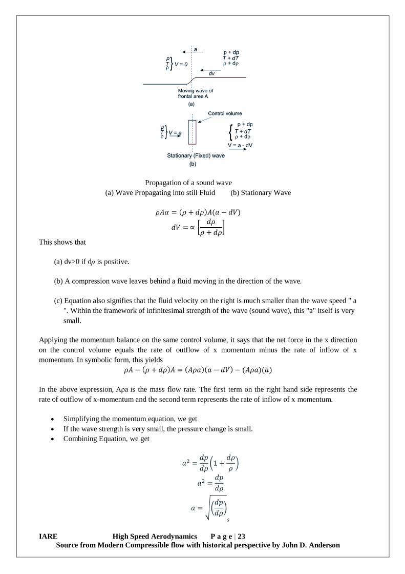
Figure shows an infinitesimal pressure pulse propagating at a speed "a" towards still fluid (V = 0)
at the left. The fluid properties ahead of the wave are p,T and ρ, while the properties behind the
wave are p+dp, T+dT and ρ+dρ. The fluid velocity dV is directed toward the left following wave
but much slower.
In order to make the analysis steady, we superimpose a velocity "a" directed towards right, on the entire
system. The wave is now stationary and the fluid appears to have velocity "a" on the left and (a - dV) on
the right. The flow in figure is now steady and one dimensional across the wave. Consider an area A on
the wave front. A mass balance gives
IARE High Speed Aerodynamics P a g e | 23
Source from Modern Compressible flow with historical perspective by John D. Anderson
Propagation of a sound wave
(a) Wave Propagating into still Fluid (b) Stationary Wave
𝜌𝐴𝛼 = (𝜌 + 𝑑𝜌)𝐴(𝑎 − 𝑑𝑉)
𝑑𝑉 = ∝ [𝑑𝜌
𝜌 + 𝑑𝜌]
This shows that
(a) dv>0 if dρ is positive.
(b) A compression wave leaves behind a fluid moving in the direction of the wave.
(c) Equation also signifies that the fluid velocity on the right is much smaller than the wave speed " a
". Within the framework of infinitesimal strength of the wave (sound wave), this "a" itself is very
small.
Applying the momentum balance on the same control volume, it says that the net force in the x direction
on the control volume equals the rate of outflow of x momentum minus the rate of inflow of x
momentum. In symbolic form, this yields
𝜌𝐴 − (𝜌 + 𝑑𝜌)𝐴 = (𝐴𝜌𝑎)(𝑎 − 𝑑𝑉) − (𝐴𝜌𝑎)(𝑎)
In the above expression, Aρa is the mass flow rate. The first term on the right hand side represents the
rate of outflow of x-momentum and the second term represents the rate of inflow of x momentum.
Simplifying the momentum equation, we get
If the wave strength is very small, the pressure change is small.
Combining Equation, we get
𝑎2 =𝑑𝑝
𝑑𝜌(1 +
𝑑𝜌
𝜌)
𝑎2 =𝑑𝑝
𝑑𝜌
𝑎 = √(𝑑𝑝
𝑑𝜌)
𝑠

IARE High Speed Aerodynamics P a g e | 24
Source from Modern Compressible flow with historical perspective by John D. Anderson
For a perfect gas, by using of 𝑃
𝜌𝛾 = 𝑐𝑜𝑛𝑠𝑡 , and P= ρRT, we deduce the speed of sound as
𝑎 = √𝛾𝑝
𝜌= √𝛾𝑅𝑇
For air at sea-level and at a temperature of 150C, a=340 m/s
1.7.2 Pressure Field Due to a Moving Source
Consider a point source emanating infinitesimal pressure disturbances in a still fluid, in which the
speed of sound is "a". If the point disturbance, is stationary then the wave fronts are concentric
spheres. As wave fronts are present at intervals of Δt.
Now suppose that source moves to the left at speed U < a. Figure shows four locations of the
source, 1 to 4, at equal intervals of time ∆t, with point 4 being the current location of the source.
At point 1, the source emanated a wave which has spherically expanded to a radius 3a∆t in an
interval of time 3Δt . During this time the source has moved to the location 4 at a distance of 3uΔt
from point 1. The figure also shows the locations of the wave fronts emitted while the source was
at points 2 and 3, respectively.
When the source speed is supersonic U > a, the point source is ahead of the disturbance and an observer
in the downstream location is unaware of the approaching source. The disturbance emitted at different
points of time is enveloped by an imaginary conical surface known as "Mach Cone". The half angle of the
cone α, is known as Mach angle and given by
sin 𝛼 = 𝑎∆𝑡
𝑈∆𝑡=
1
𝑀𝑎
𝛼 = sin−1(1/𝑀𝑎)
Since the disturbances are confined to the cone, the area within the cone is known as zone of
action and the area outside the cone is zone of silence.
An observer does not feel the effects of the moving source till the Mach Cone covers his position.

IARE High Speed Aerodynamics P a g e | 25
Source from Modern Compressible flow with historical perspective by John D. Anderson
Fig 1.2 Wave fronts emitted from a point source in a still fluid when the source speed is
(a) U = 0 (still Source) (b) U < a (Subsonic) (c) U > a (Supersonic)
It may be seen that the speed of sound is the thermodynamic property that varies from point to point.
When there is a large relative speed between a body and the compressible fluid surrounds it, then the
compressibility of the fluid greatly influences the flow properties. Ratio of the local speed (V) of the gas
to the speed of sound (a) is called as local Mach number (M).
𝑀 =𝑉
𝑎=
𝑉
√𝛾𝑅𝑇
There are few physical meanings for Mach number;
(a) It shows the compressibility effect for a fluid i.e. M<0.3 implies that fluid is incompressible.
(b) It can be shown that Mach number is proportional to the ratio of kinetic to internal energy.
(c) It is a measure of directed motion of a gas compared to the random thermal motion of the molecules.

IARE High Speed Aerodynamics P a g e | 26
Source from Modern Compressible flow with historical perspective by John D. Anderson
1.7.3 Compressible Flow Regimes
In order to illustrate the flow regimes in a compressible medium, let us consider the flow over an
aerodynamic body. The flow is uniform far away from the body with free stream velocity V∞ while the
speed of sound in the uniform stream is a∞. Then, the free stream Mach number becomes M∞ =(V∞/a∞).
The streamlines can be drawn as the flow passes over the body and the local Mach number can also vary
along the streamlines. Let us consider the following distinct flow regimes commonly dealt with in
compressible medium.
Subsonic flow : It is a case in which an airfoil is placed in a free stream flow and the local Mach number
is less than unity everywhere in the flow field. The flow is characterized by smooth streamlines with
continuous varying properties. Initially, the streamlines are straight in the free stream, but begin to deflect
as they approach the body. The flow expands as it passed over the airfoil and the local Mach number on
the top surface of the body is more than the free stream value. Moreover, the local Mach number (M) in
the surface of the airfoil remains always less than 1, when the free stream Mach number (M∞) is
sufficiently less than 1. This regime is defined as subsonic flow which falls in the range of free stream
Mach number less than 0.8.
Transonic flow: If the free stream Mach number increases but remains in the subsonic range close to 1,
then the flow expansion over the air foil leads to supersonic region locally on its surface. Thus, the entire
regions on the surface are considered as mixed flow in which the local Mach number is either less or
more than 1 and thus called as sonic pockets. The phenomena of sonic pocket is initiated as soon as the
local Mach number reaches 1 and subsequently terminates in the downstream with a shock wave across
which there is discontinuous and sudden change in flow properties. If the free stream Mach number is
slightly above unity, the shock pattern will move towards the trailing edge and a second shock wave
appears in the leading edge which is called as bow shock. In front of this bow shock, the streamlines are
straight and parallel with a uniform supersonic free stream Mach number. After passing through the bow
shock, the flow becomes subsonic close to the free stream value. Eventually, it further expands over the
airfoil surface to supersonic values and finally terminates with trailing edge shock in the downstream. The
mixed flow patterns sketched, is defined as the transonic regime.
Fig. 1.3: Illustration of compressible flow regime: (a) subsonic flow; (b & c) transonic flow; (d)
supersonic flow; (d) hypersonic flow.
Supersonic flow:In a flow field, if the Mach number is more than 1 everywhere in the domain, then it
defined as supersonic flow. In order to minimize the drag, all aerodynamic bodies in a supersonic flow,

IARE High Speed Aerodynamics P a g e | 27
Source from Modern Compressible flow with historical perspective by John D. Anderson
are generally considered to be sharp edged tip. Here, the flow field is characterized by straight, oblique
shock as shown in Fig. 1.3(d). The stream lines ahead of the shock the streamlines are straight, parallel
and horizontal. Behind the oblique shock, the streamlines remain straight and parallel but take the
direction of wedge surface. The flow is supersonic both upstream and downstream of the oblique shock.
However, in some exceptional strong oblique shocks, the flow in the downstream may be subsonic.
Hypersonic flow: When the free stream Mach number is increased to higher supersonic speeds, the
oblique shock moves closer to the body surface (Fig. 1.3-e). At the same time, the pressure, temperature
and density across the shock increase explosively. So, the flow field between the shock and body
becomes hot enough to ionize the gas. These effects of thin shock layer, hot and chemically reacting
gases and many other complicated flow features are the characteristics of hypersonic flow. In reality,
these special characteristics associated with hypersonic flows appear gradually as the free stream Mach
numbers is increased beyond 5.
As a rule of thumb, the compressible flow regimes are classified as below;
M < 0.3 (incompressible flow)
M < 1 (subsonic flow)
0.8 < M < 1.2 (transonic flow)
M > 1 (supersonic flow)
M > 5 an above (hypersonic flow)
Rarefied and Free Molecular Flow: In general, a gas is composed of large number of discrete atoms
and molecules and all move in a random fashion with frequent collisions. However, all the fundamental
equations are based on overall macroscopic behavior where the continuum assumption is valid. If the
mean distance between atoms/molecules between the collisions is large enough to be comparable in same
order of magnitude as that of characteristics dimension of the flow, then it is said to be low
density/rarefied flow. Under extreme situations, the mean free path is much larger than the characteristic
dimension of the flow. Such flows are defined as free molecular flows. These are the special cases
occurring in flight at very high altitudes (beyond 100 km) and some laboratory devices such as electron
beams.
1.8 GOVERNING EQUATIONS FOR COMPRESSIBLE FLOWS
One dimensional form of Mass conservation or Continuity Equation
Fig. 1.4 One-dimensional flow

IARE High Speed Aerodynamics P a g e | 28
Source from Modern Compressible flow with historical perspective by John D. Anderson
For steady flow Equation becomes
∯ 𝜌𝑉. 𝑑𝑠
𝑠
= 0
Applying the surface integral over the control volume of Figure, this equation becomes
−𝑃1𝑢1𝐴 + 𝑃2𝑢2𝐴 = 0
Or
𝜌1𝑢1 = 𝜌2𝑢2
For flow over the varying cross-sectional area such as nozzle and diffuser, equation modifies to
−𝜌1𝑢1𝐴1 + 𝜌2𝑢2𝐴2 = 0
One dimensional form of Momentum conservation Equation
For the steady and inviscid flow with no body forces, the Equation reduces to
∯(𝜌𝑉. 𝑑𝑠)𝑉 = ∯ 𝑃𝑑𝑠
𝑠𝑠
Above equation is a vector equation. However, since we are dealing with the one-dimensional flow, we
need to consider only the scalar x component of equation.
∯(𝜌𝑉. 𝑑𝑠)𝑢 = − ∯(𝑃𝑑𝑠)𝑥
𝑠𝑠
Considering the control volume shown in Fig (1.4), above equation transforms to,
𝜌1(−𝑢1𝐴)𝑢1 + 𝜌2(−𝑢2𝐴)𝑢2 = −(−𝑃1𝐴 + 𝑃2𝐴)
or
𝑃1 + 𝜌1𝑢12 = 𝑃2 + 𝜌2𝑢2
2
This is the momentum equation for steady inviscid one-dimensional flow.
1.8.1 One dimensional form of Conservation of Energy
Consider the control shown in Figure for steady inviscid flow without body force, and then the equation
reduces to,
∰ 𝑞𝜌𝑑𝑣 − ∯ 𝑃𝑉.
𝑠
𝑑𝑠 =
𝑣
∯ 𝜌 (𝑒 +𝑉2
2)
𝑠
𝑉. 𝑑𝑠
Let us denote the first term on left hand side of above equation by�̇� to represent the total external heat
addition in the system. Thus, above equation becomes
�̇� − ∯ 𝑃𝑉.
𝑠
𝑑𝑠 = ∯ 𝜌 (𝑒 +𝑉2
2)
𝑠
𝑉. 𝑑𝑠
Evaluating the surface integrals over the control volume in Figure, we obtain

IARE High Speed Aerodynamics P a g e | 29
Source from Modern Compressible flow with historical perspective by John D. Anderson
�̇� − (−𝑃1𝑢1𝐴 + 𝑃2𝑢2𝐴) = −𝜌1 (𝑒1 +𝑢1
2
2) 𝑢1𝐴 + 𝜌2 (𝑒2 +
𝑢22
2) 𝑢2𝐴
Or
�̇�
𝐴+ 𝑃1𝑢1 + 𝜌1 (𝑒1 +
𝑢12
2) 𝑢1 = 𝑃2𝑢2 + 𝜌2 (𝑒2 +
𝑢22
2) 𝑢2
or
�̇�
𝜌1𝑢1𝐴+
𝑃1
𝜌1+ 𝑒1 +
𝑢12
2=
𝑃2
𝜌2+ 𝑒2 +
𝑢22
2
or
�̇�
𝜌1𝑢1𝐴+ 𝑃1𝑣1 + 𝑒1 +
𝑢12
2= 𝑃2𝑣2 + 𝑒2 +
𝑢22
2
Here, �̇�/ρ1u1A is the external heat added per unit mass, q. Also, we know e + Pu = h.
Hence, above equation can be re-written as,
ℎ1 +𝑢1
2
2+ 𝑞 = ℎ2 +
𝑢22
2
This is the energy equation for steady one-dimensional flow for inviscid flow.
1.8.2 Fundamental Equations for Compressible Flow
Consider a compressible flow passing through a rectangular control volume as shown in Figure. The flow
is one-dimensional and the properties change as a function of x, from the region ‘1' to ‘2' and they are
velocity (u), pressure (p), temperature (T), density (ρ) and internal energy (e). The following assumptions
are made to derive the fundamental equations;
• Flow is uniform over left and right side of control volume.
• Both sides have equal area (A), perpendicular to the flow.
• Flow is inviscid, steady and nobody forces are present.
• No heat and work interaction takes place to/from the control volume.
Let us apply mass, momentum and energy equations for the one dimensional flow.
Conservation of Mass:
−𝑃1𝑢1𝐴 + 𝑃2𝑢2𝐴 = 0
⇒ 𝜌1𝑢1 + 𝜌2𝑢2
Conservation of Momentum:
𝜌1(−𝑢1𝐴)𝑢1 + 𝜌2(−𝑢2𝐴)𝑢2 = −(−𝑃1𝐴 + 𝑃2𝐴)

IARE High Speed Aerodynamics P a g e | 30
Source from Modern Compressible flow with historical perspective by John D. Anderson
𝑃1 + 𝜌1𝑢12 = 𝑃2 + 𝜌2𝑢2
2
Steady Flow Energy Conservation:
𝑃1
𝜌1+ 𝑒1 +
𝑢12
2=
𝑃2
𝜌2+ 𝑒2 +
𝑢22
2
ℎ1 +𝑢1
2
2+ 𝑞 = ℎ2 +
𝑢22
2
Here, the enthalpy h(=e+P/ρ) is defined as another thermodynamic property of the gas.
Fig.1.5 Schematic representation of one-dimensional flow

IARE High Speed Aerodynamics P a g e | 31
Source from Modern Compressible flow with historical perspective by John D. Anderson
UNIT II
SHOCK AND EXPANSION WAVES
2.1 DEVELOPMENT OF GOVERNING EQUATIONS FOR NORMAL SHOCK
2.1.1 Shock Waves
Let us consider a subsonic and supersonic flow past a body. In both the cases, the body acts as an
obstruction to the flow and thus there is a change in energy and momentum of the flow. The changes in
flow properties are communicated through pressure waves moving at speed of sound everywhere in the
flow field (i.e. both upstream and downstream). If the incoming stream is subsonic i.e. M∞<1; V∞< a∞,
the sound waves propagate faster than the flow speed and warn the medium about the presence of the
body. So, the streamlines approaching the body begin to adjust themselves far upstream and the flow
properties change the pattern gradually in the vicinity of the body.
In contrast, when the flow is supersonic, i.e. M∞>1; V∞> a∞, the sound waves overtake the speed of the
body and these weak pressure waves merge themselves ahead of the body leading to compression in the
vicinity of the body. In other words, the flow medium gets compressed at a very short distance ahead of
the body in a very thin region that may be comparable to the mean free path of the molecules in the
medium. Since, these compression waves propagate upstream, so they tend to merge as shock wave.
Ahead of the shock wave, the flow has no idea of presence of the body and immediately behind the
shock; the flow is subsonic.
The thermodynamic definition of a shock wave may be written as “the instantaneous compression of the
gas”. The energy for compressing the medium, through a shock wave is obtained from the kinetic energy
of the flow upstream the shock wave. The reduction in kinetic energy is accounted as heating of the gas
to a static temperature above that corresponding to the isentropic compression value. Consequently, in
flowing through the shock wave, the gas experiences a decrease in its available energy and accordingly,
an increase in entropy. So, the compression through a shock wave is considered as an irreversible
process.
Fig.2.1 Illustration of shock wave phenomena
2.1.2 Normal Shock Waves
A normal shock wave is one of the situations where the flow properties change drastically in one
direction. The shock wave stands perpendicular to the flow. The quantitative analysis of the changes

IARE High Speed Aerodynamics P a g e | 32
Source from Modern Compressible flow with historical perspective by John D. Anderson
across a normal shock wave involves the determination of flow properties. All conditions of are known
ahead of the shock and the unknown flow properties are to be determined after the shock. There is no
heat added or taken away as the flow traverses across the normal shock. Hence, the flow across the shock
wave is adiabatic(𝑞 = 0)̇ .
Fig.2.2 Schematic diagram of a standing normal shock wave
The basic one dimensional compressible flow equations can be written as below;
𝜌1𝑢1 + 𝜌2𝑢2
𝑃1 + 𝜌1𝑢12 = 𝑃2 + 𝜌2𝑢2
2
ℎ1 +𝑢1
2
2+ 𝑞 = ℎ2 +
𝑢22
2
For a calorically perfect gas, thermodynamic relations can be used,
𝑃 = 𝜌𝑅𝑇; ℎ = 𝑐𝑝𝑇; 𝑎 = √𝛾𝑝
𝜌
The continuity and momentum equations of Equation can be simplified to obtain,
𝑎12
𝛾𝑢1−
𝑎22
𝛾𝑢2= 𝑢2 − 𝑢1
Since,𝑎∗ = √𝛾𝑅𝑇∗ and𝑀∗ =𝑉
𝑎∗ , the energy equation is written as,
𝑎2
𝛾 − 1+
𝑢2
2=
𝛾 + 1
2(𝛾 − 1)𝑎∗2
𝑎2 =𝛾 + 1
2𝑎∗2 −
𝛾 − 1
2𝑢2
Both𝑎12and 𝑎2
2 can now be expressed as,

IARE High Speed Aerodynamics P a g e | 33
Source from Modern Compressible flow with historical perspective by John D. Anderson
𝑎12 =
𝛾 + 1
2𝑎∗2 −
𝛾 − 1
2𝑢1
2; 𝑎22 =
𝛾 + 1
2𝑎∗2 −
𝛾 − 1
2𝑢2
2
solve for𝑎∗2
𝑎∗2 = 𝑢1𝑢2 ⇒ 𝑀2∗ =
1
𝑀1∗
Recall the relation for M and M* and substitute in equation,
𝑀∗2 =(𝛾 + 1)𝑀2
2 + (𝛾 + 1)𝑀2
Solve for M2
𝑀22 =
1 + (𝛾−1
2) 𝑀1
2
𝛾𝑀12 − (
𝛾−1
2)
Using continuity equation and Prandtl relation, we can write,
𝜌2
𝜌1=
𝑢2
𝑢1=
𝑢12
𝑢1𝑢2=
𝑢12
𝑎∗2 = (𝑀1∗)2
Solve for density and velocity ratio across the normal shock.
𝜌2
𝜌1=
𝑢2
𝑢1=
(𝛾 + 1)𝑀12
2 + (𝛾 + 1)𝑀12
The pressure ratio can be obtained by the combination of momentum and continuity equations i.e.
𝑃2 − 𝑃1 = 𝜌1𝑢1(𝑢1 − 𝑢2) = 𝜌1𝑢12 (1 −
𝑢2
𝑢1)
𝑃2 − 𝑃1
𝑃1= 𝛾𝑢1
2 (1 −𝑢2
𝑢1)
Simplifying for the pressure ratio across the normal shock, we get,
𝑃2
𝑃1= 1 +
2𝛾
𝛾 + 1(𝑀2
2 − 1)
For a calorically perfect gas, equation of state relation can be used to obtain the temperature ratio across
the normal shock i.e.
ℎ2
ℎ1=
𝑇2
𝑇1= (
𝑃2
𝑃1) (
𝜌1
𝜌2) = [1 +
2𝛾
𝛾 + 1(𝑀1
2 − 1)] [2 + (𝛾 − 1)𝑀1
2
(𝛾 + 1)𝑀12 ]
Thus, the upstream Mach number is the powerful tool to dictating the shock wave properties. The
“stagnation properties” across the normal shock can be computed as follows;
𝑃02
𝑃01=
(𝑃02/𝑃2)
(𝑃01/𝑃1)(
𝑃2
𝑃1)
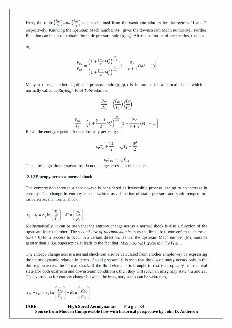
IARE High Speed Aerodynamics P a g e | 34
Source from Modern Compressible flow with historical perspective by John D. Anderson
Here, the ratios(𝑃01
𝑃1) 𝑎𝑛𝑑 (
𝑃02
𝑃2) can be obtained from the isentropic relation for the regions ‘1 and 2'
respectively. Knowing the upstream Mach number M1, gives the downstream Mach numberM2. Further,
Equation can be used to obtain the static pressure ratio (p2/p1). After substitution of these ratios, reduces
to,
𝑃02
𝑃01=
(1 +𝛾−1
2𝑀2
2)
𝛾
𝛾−1
(1 +𝛾−1
2𝑀1
2)
𝛾
𝛾−1
[1 +2𝛾
𝛾 + 1(𝑀1
2 − 1)]
Many a times, another significant pressure ratio (p02/p1) is important for a normal shock which is
normally called as Rayleigh Pitot Tube relation.
𝑃02
𝑃01= (
𝑃02
𝑃2) (
𝑃2
𝑃1)
𝑃02
𝑃2= (1 +
𝛾 − 1
2𝑀2
2)
𝛾
𝛾−1
[1 +2𝛾
𝛾 + 1(𝑀1
2 − 1)]
Recall the energy equation for a calorically perfect gas:
𝑐𝑝𝑇1 +𝑢1
2
2= 𝑐𝑝𝑇2 +
𝑢22
2
𝑐𝑝𝑇01 = 𝑐𝑝𝑇02
Thus, the stagnation temperatures do not change across a normal shock.
2.1.3Entropy across a normal shock
The compression through a shock wave is considered as irreversible process leading to an increase in
entropy. The change in entropy can be written as a function of static pressure and static temperature
ratios across the normal shock.
Mathematically, it can be seen that the entropy change across a normal shock is also a function of the
upstream Mach number. The second law of thermodynamics puts the limit that ‘entropy' must increase
(s2-s1≥ 0) for a process to occur in a certain direction. Hence, the upstream Mach number (M1) must be
greater than 1 (i.e. supersonic). It leads to the fact that M2≤1;(p2/p1≥1;(ρ2/ρ1)≥1;(T2/T1)≥1 .
The entropy change across a normal shock can also be calculated from another simple way by expressing
the thermodynamic relation in terms of total pressure. It is seen that the discontinuity occurs only in the
thin region across the normal shock. If the fluid elements is brought to rest isentropically from its real
state (for both upstream and downstream conditions), then they will reach an imaginary state ‘1a and 2a'.
The expression for entropy change between the imaginary states can be written as,

IARE High Speed Aerodynamics P a g e | 35
Source from Modern Compressible flow with historical perspective by John D. Anderson
Since, , the Equation reduces to,
Because of the fact s2>s1, Equation implies that p02< p01. Hence, the stagnation pressure always decreases
across a normal shock.
2.1.4 Normal shock relations
It had already been discussed that the subsonic flow is pre-warned and supersonic flow is not. The reason
behind this fact is that, any small amplitude disturbance travels with acoustic speed, however speed of
fluid particle is more than the speed of sound in case of supersonic flows. Therefore the message of
presence of the obstacle cannot propagate upstream. Hence a messenger gets developed in front of the
obstacle to warn the flow in order to avoid its direct collision with the obstacle. This messenger is called
as shock. In the presence of normal shock, fluid velocity decreases to the extent where flow Mach
number behind the shock attains value below one. Due to this subsonic speed attainment of the flow, it
becomes aware about the presence of the obstacle well in advance in the narrow space between shock
and obstacle. Herewith we will deal for computation of flow properties behind the normal shock.
In the presence of a general obstacle the shock pattern.
Fig. 2.3 Shock pattern for a blunt or bluff obstacle
The shock for the stagnation streamline can be considered as normal to it. Therefore we can use the
earlier derived 1D flow relations along with the assumptions of flow steady, adiabatic and inviscid flow.
Consider a small control volume around normal shock for application of these relations between two
stations of the control volume, mainly, inlet and outlet.
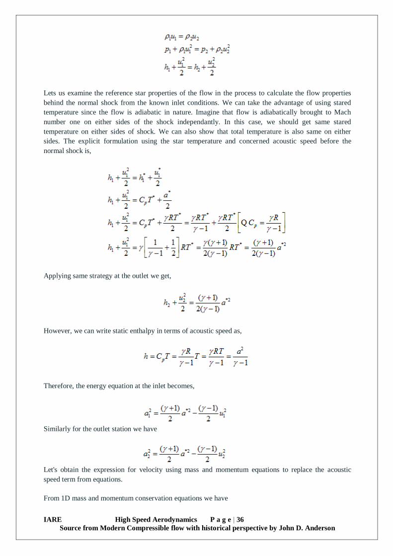
IARE High Speed Aerodynamics P a g e | 36
Source from Modern Compressible flow with historical perspective by John D. Anderson
Lets us examine the reference star properties of the flow in the process to calculate the flow properties
behind the normal shock from the known inlet conditions. We can take the advantage of using stared
temperature since the flow is adiabatic in nature. Imagine that flow is adiabatically brought to Mach
number one on either sides of the shock independantly. In this case, we should get same stared
temperature on either sides of shock. We can also show that total temperature is also same on either
sides. The explicit formulation using the star temperature and concerned acoustic speed before the
normal shock is,
Applying same strategy at the outlet we get,
However, we can write static enthalpy in terms of acoustic speed as,
Therefore, the energy equation at the inlet becomes,
Similarly for the outlet station we have
Let's obtain the expression for velocity using mass and momentum equations to replace the acoustic
speed term from equations.
From 1D mass and momentum conservation equations we have

IARE High Speed Aerodynamics P a g e | 37
Source from Modern Compressible flow with historical perspective by John D. Anderson
ρ1u1 = ρ2u2
p1 + ρ1u12 = p2 + ρ2u2
2
Therefore,
Using, above equation transforms to
Rearranging the terms of above equation, we get
A further rearrangement gives
Necessary rearrangement for the above equation is as given,

IARE High Speed Aerodynamics P a g e | 38
Source from Modern Compressible flow with historical perspective by John D. Anderson
This expression shows that, M1*2 and M2
*2 are reciprocal of each other for a normal shock. This equation
is called as Prandtl’s relation for normal shock which can be used to prove that Mach number becomes
subsonic behind the normal shock
Shock waves are highly localized irreversibilities in the flow.
Within the distance of a mean free path, the flow passes from a supersonic to a subsonic state, the
velocity decreases suddenly and the pressure rises sharply. A shock is said to have occurred if
there is an abrupt reduction of velocity in the downstream in course of a supersonic flow in a
passage or around a body.
Normal shocks are substantially perpendicular to the flow and oblique shocks are inclined at any
angle.
Shock formation is possible for confined flows as well as for external flows.
Normal shock and oblique shock may mutually interact to make another shock pattern.
Fig.2.4 Different type of Shocks

IARE High Speed Aerodynamics P a g e | 39
Source from Modern Compressible flow with historical perspective by John D. Anderson
Figure below shows a control surface that includes a normal shock.
Fig 2.5 One Dimensional Normal Shock
The fluid is assumed to be in thermodynamic equilibrium upstream and downstream of the shock, the
properties of which are designated by the subscripts 1 and 2, respectively.
Continuity equation can be written as
where G is the mass velocity kg/ m2 s, and is mass flow rate
From momentum equation, we can write
where p + ρV2 is termed as Impulse Function .
The energy equation is written as
where h0 is stagnation enthalpy.
From the second law of thermodynamics, we know
To calculate the entropy change, we have

IARE High Speed Aerodynamics P a g e | 40
Source from Modern Compressible flow with historical perspective by John D. Anderson
For an ideal gas
For an ideal gas the equation of state can be written as
For constant specific heat, the above equation can be integrated to give
Above equations are the governing equations for the flow of an ideal gas through normal shock.
If all the properties at state 1 (upstream of the shock) are known, then we have six unknowns T2, P2, ρ2,
V2, h2, s2in these five equations.
We know relationship between h and T for an ideal gas,dh = cPdT.
For an ideal gas with constant specific heats,
Thus, we have the situation of six equations and six unknowns.
If all the conditions at state "1"(immediately upstream of the shock) are known, how many possible states
2 (immediate downstream of the shock) are there? The mathematical answer indicates that there is a
unique state 2 for a given state 1.
2.1.5 Stationary and Moving Normal Shock Waves
The easiest way to analyze a normal shock is to consider a control surface around the wave. The
continuity equation, the momentum equation and the energy equation have already been discussed
earlier. The energy equation can be simplified for an ideal gas as
T01=T02
By making use of the equation for the speed of sound equation and the equation of state for ideal gas
equation, the continuity equation can be rewritten to include the influence of Mach number as:
Introducing the Mach number in momentum equation, we have
Therefore,
Rearranging this equation for the static pressure ratio across the shock wave, we get
As already seen, the Mach number of a normal shock wave is always greater than unity in the upstream
and less than unity in the downstream; the static pressure always increases across the shock wave.
IARE High Speed Aerodynamics P a g e | 41
Source from Modern Compressible flow with historical perspective by John D. Anderson
The energy equation can be written in terms of the temperature and Mach number using the stagnation
temperature relationship as
Substituting Equation yields the following relationship for the Mach numbers upstream and downstream
of a normal shock wave:
Then, solving this equation for Ma2 as a function of Ma1 we obtain two solutions. One solution is trivial
Ma2 = Ma1, which signifies no shock across the control volume. The other solution is
𝑀𝑎1 = 1 In Equation results in𝑀𝑎2 = 1
Above Equations also show that there would be no pressure or temperature increase across the shock. In
fact, the shock wave corresponding to Ma1 = 1 is the sound wave across which, by definition, pressure
and temperature changes are infinitesimal. Therefore, it can be said that the sound wave represents a
degenerated normal shock wave. The pressure, temperature and Mach number (Ma2) behind a normal
shock as a function of the Mach number Ma1, in front of the shock for the perfect gas can be represented
in a tabular form.
2.2 APPLICATION TO AIRCRAFTS
Air intakes for supersonic aircraft present an excellent example for the application of the theory of shock
waves in steady flow. This chapter describes the operation of such devices given that it is only an
introduction to the aerodynamics of air intakes whose design has many aspects that will not be mentioned
here. We know that the propulsion of aircraft is provided by the so-called propulsion nacelle, or more
simply the nacelle, which brings together the various elements contributing to the propulsion, namely:
the air intake, capturing air to feed the engine;
the engine that can be a turbojet, a ramjet, or even a scramjet engine for air breathing hypersonic
vehicles;
a possible reheat duct or afterburner, where kerosene is burnt downstream of the engine in order
to provide extra thrust; and
the exhaust nozzle whose aerodynamics.
The engines of current airliners additionally have a fan, arranged in front of the compressor and drawing
an airflow that does not cross the compressor–turbine set. The operation of the fan is characterized by the
bypass ratio, a ratio of the total drawn airflow and the airflow through the compressor. This bypass ratio
is around 10 for modern engines. Engines for combat aircraft and missiles have no fan.

IARE High Speed Aerodynamics P a g e | 42
Source from Modern Compressible flow with historical perspective by John D. Anderson
2.3 SUPERSONIC WIND TUNNEL
Fig 2.6 Schematic of indraft tunnel
Following are the components of this tunnel.
1. Air inlet
2.Settling chamber
3.Nozzle
4.Sonic throat
5.Test-section
6.Second throat
7.Diffuser
8.Vacuum chamber.
Some blow down tunnels, called as in draft tunnels, do not use a high pressure chamber, but use
atmosphere as the reservoir. The in draft tunnel uses the low pressure (vacuum) chamber downstream of
the test section to produce flow. During the operation of this tunnel, air from the atmosphere enters the
nozzle and gets expanded to require Mach number defined by the area ratio of the nozzle. Further flow of
the air from the test section, second throat decelerates the air and let it fill the vacuum chamber. The main
advantage of this configuration is that the conditions in the inlet remain constant and there is no need for
a pressure regulator. The disadvantage is that the pressure ratio across the test section is usually lower
than a closed configuration and therefore the maximum Mach number (M>2) is not possible.

IARE High Speed Aerodynamics P a g e | 43
Source from Modern Compressible flow with historical perspective by John D. Anderson
2.3.1 Closed Continuous Wind Tunnel
Fig 2.7 Schematic of closed circuit continuous wind tunnel
Following are the parts of this wind tunnel.
1. Air compressor
2.Dryer
3.Dry air storage
4.Return passage
5.Driver motor
6.Compressor
7.Cooler
8.Settling chamber
9.Nozzle
10.Test-section
11.Diffuser
In the closed return tunnel, air is passed from the exit of the test section back to the inlet by a series of
turning vanes at the corner of the tunnel. Exiting the diffuser, the air is returned to the nozzle and back
through the test section. Air is continuously circulated through the duct work of the closed return tunnel.
To prevent condensation in the test section because of low pressure, the air entering the tunnel is often
passed over a dryer bed. There is usually an additional throat placed in the tunnel downstream of the test
section to decelerate the supersonic flow to subsonic. The continuous closed-circuit supersonic tunnel has
some advantages and some disadvantages relative to the intermittent tunnel. Advantages of the closed
return tunnels include longer run times relative to the blow down tunnel, superior flow quality in the test
section, flow turning vanes in the corner and flow straighteners near the test section ensure relatively
uniform flow in the test section, lesser noisy operation, the test section can be designed for high Mach
numbers (M>4) and large-size models, low operating costs. Also once the air is circulating in the tunnel,
the fan and motor only needs to overcome losses along the wall and through the turning vanes. The fan
does not have to constantly accelerate the air.On the same grounds disadvantages of the closed return
tunnels include higher construction cost because of the added vanes and ducting. This tunnel must be
designed to purge exhaust products that accumulate in the tunnel.

IARE High Speed Aerodynamics P a g e | 44
Source from Modern Compressible flow with historical perspective by John D. Anderson
2.3.2 Supersonic Diffuser
Supersonic diffuser with second throat should be designed critically because increasing diffuser
efficiency will lower the power requirement considerably. The first throat is the one upstream of the test-
section through which the flow accelerates. An ideal diffuser would be characterized by an isentropic
compression to lower velocities. This situation is sketched in Figure 2.8. Because the flow is isentropic
the stagnation pressures at both ends of the diffuser would be equal. But it is extremely difficult to slow a
supersonic flow without generating shock waves in the process. Moreover, in practical situation, the flow
is viscous. As a result there will be an entropy increase within the boundary layers on the walls of the
diffuser.
Fig 2.8 Schematic of ideal diffuser
1. An actual supersonic diffuser is sketched in fig 2.8. Here, the incoming flow is slowed by a series of
reflected oblique shocks, first in a convergent section and then in a constant area throat (called as
second throat). Due to the interaction of shock waves with the boundary layer near the wall, the
reflected shock pattern eventually weakens and becomes diffused. Finally, the subsonic flow
downstream of the constant area throat is further slowed by moving through a divergent section.
Schematic of ideal diffuser
2. It may be shown that a shock wave in the converging portion of the second throat would be
unstable, and in practice the second-throat Mach number is chosen large enough for the
breakdown shock system to be located well downstream of the throat, to ensure stability under all
operating conditions. When the tunnel is started up, the second throat must be rather larger than
the first throat in order to choke first, so that supersonic flow can be established in the test-
section.
2.4 Shock Tube
The shock tube is a simple duct closed at both ends. A diaphragm divides this duct into two
compartments called as driver and driven sections. Driver section of the shock tube is the high pressure
section which is supplied by the high pressure gas from the reservoir. Driven section of the shock tube is

IARE High Speed Aerodynamics P a g e | 45
Source from Modern Compressible flow with historical perspective by John D. Anderson
the low pressure section which contains the low pressure driven gas. These two sections are separated by
a metal diaphragm.
2.4.1 Working of Shock Tube
Typical shock tube experimental set up is as shown in Figure. A high pressure driver gas reservoir is
connected with the driver section. However a vacuum pump is connected to the driven section to arrive at
the accurate driven section pressure. Pressure sensors are generally mounted along the driven tube for
pressure measurement. These pressure sensors are connected to the data acquisition system.
2.4.2 Operating steps for this set up are as follows.
1. Set the metal diaphragm between the driver and driven section.
2. Fill the driven gas in the driven section from the driven gas reservoir. This step is not required
for case of air as the driven gas.
3. Set the required pressure in the driven section using vacuum pump.
4. Start filling the driver gas (say helium) in the driver section from the high pressure reservoir.
Fig 2.9 Schematic of the shock tube
Metal diaphragm bursts at a particular driver and driven gas pressure difference. Dynamics of operation
of shock tube after diaphragm burst is shown in steps in the following Fig.2.10.

IARE High Speed Aerodynamics P a g e | 46
Source from Modern Compressible flow with historical perspective by John D. Anderson
(a) On set of diaphragm burst.
(b) Propagation of shock, expansion and contact surface in the shock tube
(c) Reflection of shock and expansion from the ends of the shock tube
Fig.2.10 Motion of various waves inside the shock tube
Thus shock tube gets operated solely by slowly increasing the driver gas pressure for a given driven
pressure until the diaphragm gets ruptured. Burst of the diaphragm creates compression waves which
propagate in the driven section and expansion waves traversing in the driver section. (Similar experience
can be gained individually for compression and expansion in a tube with fixed and movable in presence
of a piston. Sudden motion of the piston towards the closed end creates compression wave in the tube and
sudden motion of the piston away from the closed end sets expansion of the inner fluid). However, in a
short interval of time, compression waves coalesce to form the shock wave which propagate in the driven
section. The stationary low pressure driven gas raises its pressure and temperature on arrival of the shock
wave. Driver gas at the same time encounters the expansion in the presence of expansion waves.
Moreover, the driver and driven gases do not mix due to the presence of contact surface which moves in
the driven section. Thus contact surface separates the driver and driven gases and provides the position of
diaphragm. The pressure and velocity are same across the contact surface. Both the expansion fan and
shock reflect from the closed ends of the shock tube. Reflected shock cancels the motion of the driven
fluid initiated by the primary shock. The strength of the shock wave and expansion fan thus produced
depends on the initial pressure ratio across the diaphragm and the physical properties of the gases in the
driver and driven sections. Higher the strength of the primary shock more is its speed in the shock tube
which intern increases the pressure and temperature rise across it along with the pressure rise across the
reflected shock.

IARE High Speed Aerodynamics P a g e | 47
Source from Modern Compressible flow with historical perspective by John D. Anderson
Following are the notations of the regions between different waves in the shock tube
Region 1: This is the region infront of the primary shock.
Region 2: It is the region between contact surface and primary shock.
Region 3: This is the region between tail of the expansion fan and contact surface.
Region 4: It is the region ahead of the leading expansion wave.
Region 5: It is the region behind the reflected shock.
Fig 2.11 Space time diagram for a typical shock tube
2.4.3 Applications of shock tube:
Shock tube is very useful equipment and can be implemented for various applications in its various
variants. Shock tube in its simplest format is used for the external flow aerodynamics studies in the
higher subsonic, transonic and lower supersonic Mach numbers. Higher diameter tubes are advisable in
these cases to avoid the domination of viscous effects. For the experimentation in supersonic or
hypersonic flow regimes, driven tube end is connected to a convergent divergent nozzle along with the
test section and dump tank to comprise a shock tunnel. This formation helps to expand the stagnant gas
behind the reflected shock through the nozzle to achieve high speed flow in the test section. Shock tube
can also be used for chemical kinetic studies for measurement of reaction rates. Use of shock tube for
contact less drug delivery has also been thought for its application in medical sciences.

IARE High Speed Aerodynamics P a g e | 48
Source from Modern Compressible flow with historical perspective by John D. Anderson
2.5 Shock Polar
In this section we are going to discuss about the graphical representation of pre and post shock
velocities. Consider the supersonic flow of Mach number M1 passing over a wedge of deflection angle θ.
Fig 2.12 Supersonic flow over a wedge
Let Vx be the component of velocity in x-direction while Vy be the component of velocity in y direction.
Hence Vx1 is the x-direction velocity component for upstream velocity and Vx2 is the x-direction velocity
component for post shock velocity. Similarly Vy1 and Vy2 are the y-direction velocity component for
upstream and post shock velocities respectively. If the upstream velocity is parallel to x axis then Vy1 is
equal to zero since Vx1 is equal to V1. Now let’s plot velocities along their respective directions. Here the
resultant velocity V1 is parallel to x axis while V2 makes an angle θ with x-axis, which is the flow
deflection angle.
Fig 2.13 Velocity plot for shocked flow
Now if we increase the deflection angle then Vx2 will decrease and Vy2 will increase since in such cases
resultant velocity V2 will have to make an increased angle θ with the x-axis. Figure represents the same
process. In the same way if we change the wedge angle for all possible attached shock solutions and join
them together then such a plot is called as hodograph.

IARE High Speed Aerodynamics P a g e | 49
Source from Modern Compressible flow with historical perspective by John D. Anderson
Fig 2.14 Velocity plot for various shocked flows
In the same way we can plot for various free stream Mach number for all the possible deflection angles.
However, if we increase the freestream Mach number by increasing free stream velocity then it becomes
impossible to plot such a graph when Vx1 becomes ∞ for M1 equal to ∞. To make such a plot possible,
lets divide x axis and y axis by a* which is the reference or stared quantity. This non-dimensionalisation
makes it possible to represent Vx1 since it will be represented by M1*. We can divide by a* to post shock
velocities as well, since a* is constant in the flow field for an adiabatic flow. Hence V2 gets transformed
to M2* which will make an angle equal to the flow deflection angle with the x-axis. This plot is called as
shock polar. Such a shock polar can be plotted for very high Mach numbers M1 also due to the fact that,
if M1 is equal to ∞, M1* is equal to 2.54. Therefore this plot is equally helpful for representing the pre
and post shock velocities, flow deflection angle and the shock angle.
Fig 2.15 Typical Shock Polar

IARE High Speed Aerodynamics P a g e | 50
Source from Modern Compressible flow with historical perspective by John D. Anderson
2.5.1 Analysis of Shock Polar
Shock polar can be used as a tool to evaluate the post shock properties from known pre shock conditions.
We can calculate a* and hence M1* which is the required pre shock input condition from the known
freestream conditions. Hence using flow deflection angle θ and M1*, we can evaluate the post shock
condition as, M2* using a given shock polar. Consider a shock polar given in Figure. Any line, say OXY,
drawn from origin which intersects the given shock polar at two locations, X and Y. Point Y of line
OXY represents higher value of M2* than the point X. Hence point Y represents the weak shock solution
while point X on shock polar represents the strong shock solution. Angle made by line OXY gives the
flow deflection angle. To find out the shock angle, we have to draw a line AY and extend the same same
till it intersects a line (OZ) drawn from the origin at 90 degree. The angle made by line OZ with x-axis is
the shock angle since this arrangement satisfies the constraint of equality of component of velocity
parallel to the shock before and after the shock. If we draw any line OM, tangent to the shock polar, then
the angle made by the line OM with x-axis represents maximum deflection angle possible for the given
freestream Mach number. If we draw a circle of radius equal to a* then such a circle cuts the shock polar
at N which represents the Mach number equal 1 behind the shock.
Fig 2.17 Shock polar for various Mach numbers
2.5.2 Applications of P-θ diagram
Pressure-deflection diagram is very useful for understanding various flow features like shock-shock
interaction, shock reflection etc. Therefore the main objective of working with this diagram is to
understand the deflection of flow which encounters various shocks. Consider a supersonic flow
experiencing two left running shock waves..
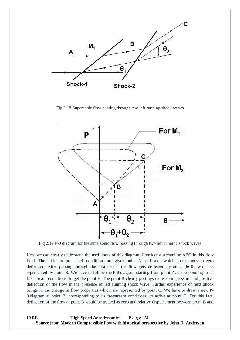
IARE High Speed Aerodynamics P a g e | 51
Source from Modern Compressible flow with historical perspective by John D. Anderson
Fig 2.18 Supersonic flow passing through two left running shock waves
Fig 2.19 P-θ diagram for the supersonic flow passing through two left running shock waves
Here we can clearly understand the usefulness of this diagram. Consider a streamline ABC in this flow
field. The initial or pre shock conditions are given point A on P-axis which corresponds to zero
deflection. After passing through the first shock, the flow gets deflected by an angle θ1 which is
represented by point B. We have to follow the P-θ diagram starting from point A, corresponding to its
free stream conditions, to get the point B. The point B clearly portrays increase in pressure and positive
deflection of the flow in the presence of left running shock wave. Further experience of next shock
brings in the change in flow properties which are represented by point C. We have to draw a new P-
θ diagram at point B, corresponding to its freestream conditions, to arrive at point C. For this fact,
deflection of the flow at point B would be treated as zero and relative displacement between point B and
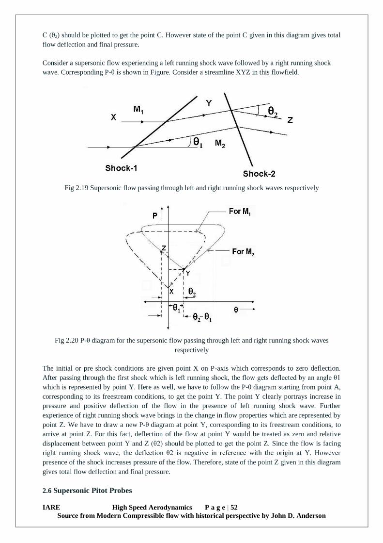
IARE High Speed Aerodynamics P a g e | 52
Source from Modern Compressible flow with historical perspective by John D. Anderson
C (θ2) should be plotted to get the point C. However state of the point C given in this diagram gives total
flow deflection and final pressure.
Consider a supersonic flow experiencing a left running shock wave followed by a right running shock
wave. Corresponding P-θ is shown in Figure. Consider a streamline XYZ in this flowfield.
Fig 2.19 Supersonic flow passing through left and right running shock waves respectively
Fig 2.20 P-θ diagram for the supersonic flow passing through left and right running shock waves
respectively
The initial or pre shock conditions are given point X on P-axis which corresponds to zero deflection.
After passing through the first shock which is left running shock, the flow gets deflected by an angle θ1
which is represented by point Y. Here as well, we have to follow the P-θ diagram starting from point A,
corresponding to its freestream conditions, to get the point Y. The point Y clearly portrays increase in
pressure and positive deflection of the flow in the presence of left running shock wave. Further
experience of right running shock wave brings in the change in flow properties which are represented by
point Z. We have to draw a new P-θ diagram at point Y, corresponding to its freestream conditions, to
arrive at point Z. For this fact, deflection of the flow at point Y would be treated as zero and relative
displacement between point Y and Z (θ2) should be plotted to get the point Z. Since the flow is facing
right running shock wave, the deflection θ2 is negative in reference with the origin at Y. However
presence of the shock increases pressure of the flow. Therefore, state of the point Z given in this diagram
gives total flow deflection and final pressure.
2.6 Supersonic Pitot Probes

IARE High Speed Aerodynamics P a g e | 53
Source from Modern Compressible flow with historical perspective by John D. Anderson
2.6.1 Measurements of Flow Velocity
In most of the cases, the flow velocity is obtained through simultaneous measurement of static and
stagnation pressures using a Prandtl Pitot Static probe. It has opening at the nose for stagnation pressure
communications while several number of equal size holes are made around the circumference of the
probe at the location downstream of the nose. The difference pressure gives the dynamic pressure.
Further, Bernoulli equation can be applied to calculate the flow velocity.
Now, replace the integral of Equation with the isentropic relation for gases;
where, P, ρ and V are the pressure, density and velocity, respectively, z is the elevation difference, ϒ is
the specific heat ratio and C is a constant. Combine Equation and simplify to obtain the Bernoulli equation for one-dimensional frictionless isentropic flow for compressible fluid.
Apply Equation along a stream line at the location of stagnation point and any desired location to obtain
the flow velocity.
The subscripts, 0 and ∞ refer to stagnation and free stream conditions, respectively. Had the flow been
incompressible, the density term in Equation becomes constant quantity and the stagnation and static
pressure difference is expressed as follows:
Fig2.21 Prandtl Pitot static probe for simultaneous measurement
2.6.2 Measurements for Subsonic and Supersonic Flows

IARE High Speed Aerodynamics P a g e | 54
Source from Modern Compressible flow with historical perspective by John D. Anderson
The flow Mach number is one of the important parameter for subsonic and supersonic flows. All the
flow parameters and their variations are the functions of local Mach number (M). The pressure
measurements are one of the common practices to determine the Mach number. In subsonic flow, the
simultaneous measurement of static(P) and stagnation pressures (p0)using a Prandtl Pitot Static tube are
made in a similar way as shown in Figure. Subsequently, the isentropic relation is used to determine the
flow Mach number.
𝑃0
𝑃∞= (1 +
𝛾 − 1
2𝑀∞
2 )
𝛾
𝛾−1
The characteristic feature of a supersonic flow is the formation of a shock wave. So, the introduction of
a Pitot probe into the flow stream, leads to a detached bow shock. Due to this shock wave at certain
distance from the measurement location, the stagnation pressure located indicated by the probe will be
much higher than the stagnation pressure of the free stream. For the stagnation stream lines, the curved
shock is normal to the free stream and the measured value represents the stagnation pressure downstream
of the normal shock (P02). While conducting experiment, the static pressure (P∞) of the free stream
(upstream of the shock) is also measured simultaneously by any of the methods. However, the static
pressure measurement must be done far upstream of the shock so that its influence on the measurement
will be minimized. The Mach number relation connecting the static and stagnation pressure
measurements is expressed by Rayleigh-Pitot formula for supersonic flows.
𝑃02
𝑃∞=
(𝛾−1
2𝑀∞
2 )
𝛾
𝛾−1
(2𝛾
𝛾+1𝑀∞
2 −𝛾−1
𝛾+1)
1
𝛾−1
The Rayleigh-Pitot formula with air as free stream is presented graphically in figure. The dynamic
pressure(Pd)obtained from static pressure and the Mach number is then given by the following
expression.
𝑃𝑑
𝑃∞=
𝛾𝑀∞2
2
Thus, the Mach number calculation through static and stagnation measurements gives complete
information of a supersonic flow field.
Fig 2.22 Detached shocks ahead of the measuring pressure probe in a supersonic flow.

IARE High Speed Aerodynamics P a g e | 55
Source from Modern Compressible flow with historical perspective by John D. Anderson
Fig 2.22 Mach number determination from Pitot tube measurement in a supersonic flow
2.6.3 Sonic Nozzle: It is an obstruction device often used to measure high flow rates for gases. When the
flow rate is sufficiently high, the pressure differential is also expected to be large. Under this condition, a
sonic flow condition is achieved at the minimum flow area and the flow is said to be choked. Such a
device is known as sonic nozzle. In this case, the flow rate takes the maximum value for a given inlet
condition. If this inlet refers to a reservoir pressure(p0), temperature(T0) and the flow is said to be choked
at certain area(A*), then the pressure at this location(P*) can be obtained from isentropic relation,
This relation is known as critical pressure ratio for a choked nozzle. The choked mass flow rate can be
obtained by the following expression,
By designing the geometric parameter of a sonic nozzle, it is possible to achieve the discharge
coefficient up to 0.97 corresponding to theoretical expression of flow rate.
A pitot probe in a supersonic stream will have a bow shock ahead of it. This complicates
theflowmeasurement,sincethebowshockwillcauseadropinthetotalpressure,frompo1 to po2 , the latter
being sensed by the pitot port. It’s useful to note that the shock will also cause a drop in ρo, but ho will
notchange.
The pressures and Mach number immediately behind the shock are related by
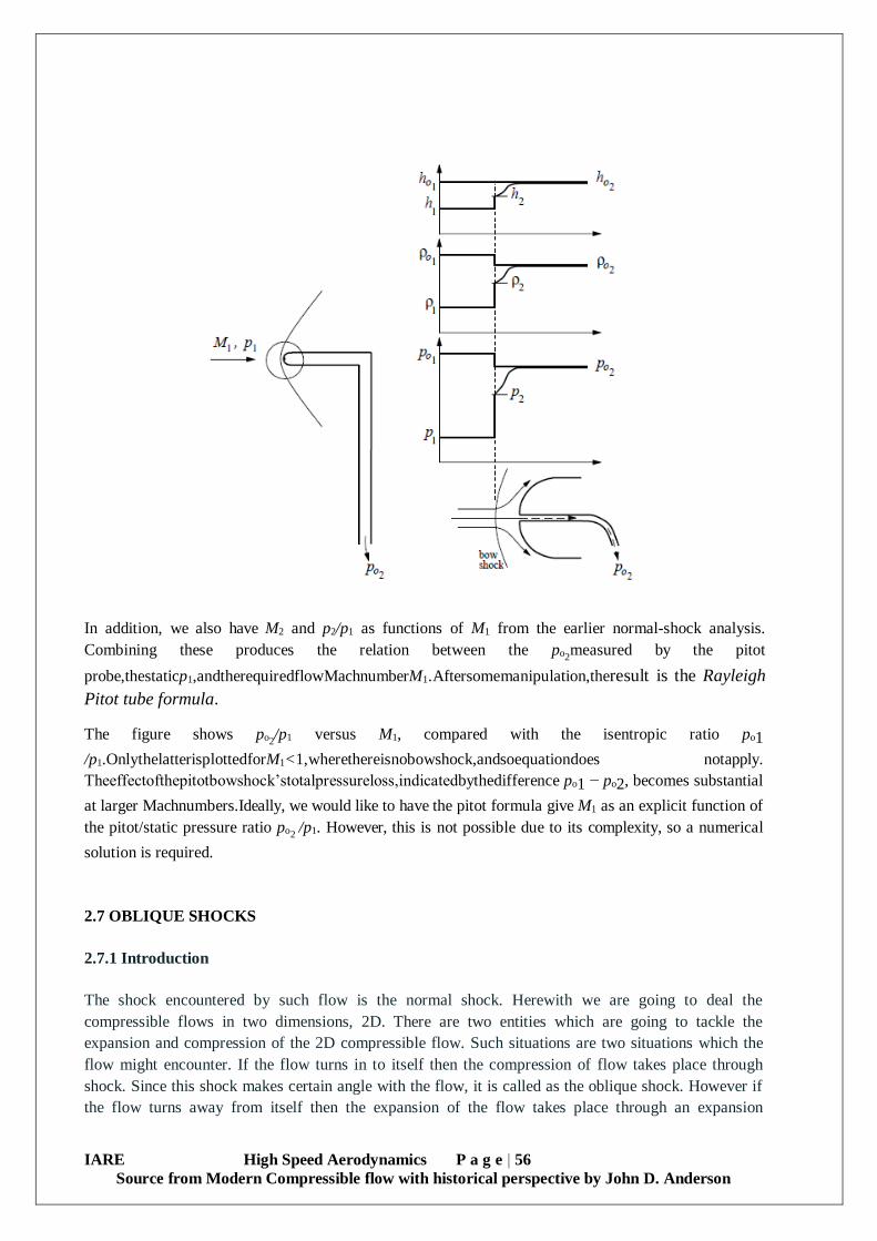
IARE High Speed Aerodynamics P a g e | 56
Source from Modern Compressible flow with historical perspective by John D. Anderson
In addition, we also have M2 and p2/p1 as functions of M1 from the earlier normal-shock analysis.
Combining these produces the relation between the po2measured by the pitot
probe,thestaticp1,andtherequiredflowMachnumberM1.Aftersomemanipulation,theresult is the Rayleigh
Pitot tube formula.
The figure shows po2/p1 versus M1, compared with the isentropic ratio po1
/p1.OnlythelatterisplottedforM1<1,wherethereisnobowshock,andsoequationdoes notapply.
Theeffectofthepitotbowshock’stotalpressureloss,indicatedbythedifference po1 − po2, becomes substantial
at larger Machnumbers.Ideally, we would like to have the pitot formula give M1 as an explicit function of
the pitot/static pressure ratio po2 /p1. However, this is not possible due to its complexity, so a numerical
solution is required.
2.7 OBLIQUE SHOCKS
2.7.1 Introduction
The shock encountered by such flow is the normal shock. Herewith we are going to deal the
compressible flows in two dimensions, 2D. There are two entities which are going to tackle the
expansion and compression of the 2D compressible flow. Such situations are two situations which the
flow might encounter. If the flow turns in to itself then the compression of flow takes place through
shock. Since this shock makes certain angle with the flow, it is called as the oblique shock. However if
the flow turns away from itself then the expansion of the flow takes place through an expansion

IARE High Speed Aerodynamics P a g e | 57
Source from Modern Compressible flow with historical perspective by John D. Anderson
fan. Deriving various relations for angles or properties ratios for the two dimensional compressible
flows in the presence of shock or expansion fan is the central objective here onwards.
Fig 2.23 Supersonic flow turning into itself in the presence of shock
Fig 2.24 Supersonic flow turning away from itself in the presence of expansion fan
The main reason of having shock or expansion fan at the deflection corners is to deflect the flow
accordingly so as to maintain its parallelism with the wall in order to avoid the direct collision.
Therefore the angle of shock with the wall or freestream velocity will be dependant on flow deflection
angle and freestream velocity.
2.7.2 Mach Wave
Let’s consider a train traveling along its track from location A to location B. If it makes a beep sound
while leaving station A and at intermediate locations C and D then the sound wave travels spherically
out with the velocity (say) 'a' m/s. The distance traveled by the sound waves originated from A,C and D
locations are given by the circles drawn, considering respective points as centers. Now if the speed of
the train is less than acoustic velocity (a), say v m/s, then the train will always remain inside the circles.
This statement also means that the distance travels by the train in some time interval is always lower
than the distance traveled by the acoustic wave in the same time interval. Now if we consider the speed
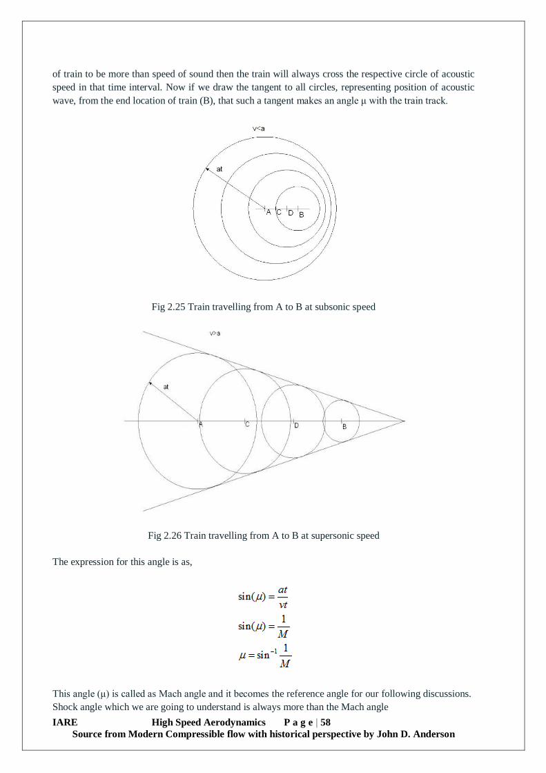
IARE High Speed Aerodynamics P a g e | 58
Source from Modern Compressible flow with historical perspective by John D. Anderson
of train to be more than speed of sound then the train will always cross the respective circle of acoustic
speed in that time interval. Now if we draw the tangent to all circles, representing position of acoustic
wave, from the end location of train (B), that such a tangent makes an angle μ with the train track.
Fig 2.25 Train travelling from A to B at subsonic speed
Fig 2.26 Train travelling from A to B at supersonic speed
The expression for this angle is as,
This angle (μ) is called as Mach angle and it becomes the reference angle for our following discussions.
Shock angle which we are going to understand is always more than the Mach angle
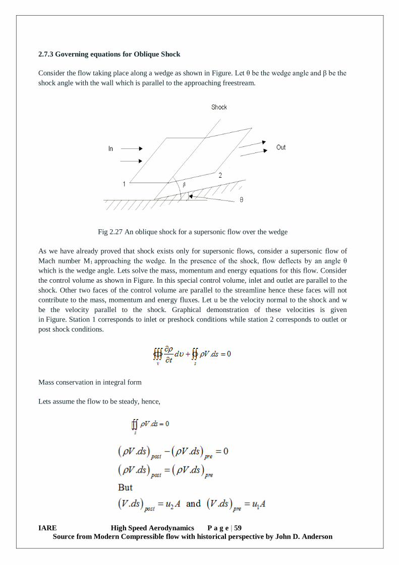
IARE High Speed Aerodynamics P a g e | 59
Source from Modern Compressible flow with historical perspective by John D. Anderson
2.7.3 Governing equations for Oblique Shock
Consider the flow taking place along a wedge as shown in Figure. Let θ be the wedge angle and β be the
shock angle with the wall which is parallel to the approaching freestream.
Fig 2.27 An oblique shock for a supersonic flow over the wedge
As we have already proved that shock exists only for supersonic flows, consider a supersonic flow of
Mach number M1 approaching the wedge. In the presence of the shock, flow deflects by an angle θ
which is the wedge angle. Lets solve the mass, momentum and energy equations for this flow. Consider
the control volume as shown in Figure. In this special control volume, inlet and outlet are parallel to the
shock. Other two faces of the control volume are parallel to the streamline hence these faces will not
contribute to the mass, momentum and energy fluxes. Let u be the velocity normal to the shock and w
be the velocity parallel to the shock. Graphical demonstration of these velocities is given
in Figure. Station 1 corresponds to inlet or preshock conditions while station 2 corresponds to outlet or
post shock conditions.
Mass conservation in integral form
Lets assume the flow to be steady, hence,

IARE High Speed Aerodynamics P a g e | 60
Source from Modern Compressible flow with historical perspective by John D. Anderson
(ρu)2 = (ρu)1 or ρ1u1 = ρ2u2
Hence,
This is the mass conservation equation for oblique shock conditions expressed in terms of velocities
normal to the shock.
Now consider the momentum conservation equation for the same flow. Since momentum is the vector
equation, we have to consider, two equations, viz, normal and parallel to the shock. Let’s initially
consider the momentum equation in integral form for inviscid flow.
For steady flow,this equation becomes,
Now consider the momentum equation in the direction parallel to the shock wave. Since there is no
pressure difference in this direction, the right hand side will be zero. Hence,
but using mass conservation Equation we can re-write it as,
(w)pre = (w)post or w1 = w2
This expression clearly suggests that velocity parallel to the shock remains conserved.
Now consider the momentum equation normal to the shock.

IARE High Speed Aerodynamics P a g e | 61
Source from Modern Compressible flow with historical perspective by John D. Anderson
(p + ρu2)post = (p + ρu2)post
Or
p1 + ρ1u12 = p2 + ρ2u2
2
We can clearly see that the momentum equation looks exactly same as that for the normal shock
relations. Here u is the velocity normal to the shock. Therefore only velocity component normal to the
shock wave is responsible for the change in momentum since momentum and velocity tangential to
shock are conserved.
2.7.4 θ-β-M relation
It has been already observed that the Mach number normal to the shock is responsible for all the
property variations for given shock angle. However this shock angle can be easily calculated from the
upstream or freestream Mach number for given wedge or deflection angle. Consider the same control
volume shown in Figure. Relation between velocities and angles before and after the shocks are,
Before the shock
After the shock
But we know that,
w1 = w2
Hence,
But
ρ1u1 = ρ2u2 hence,
Therefore,
From density ratio Equation, we have
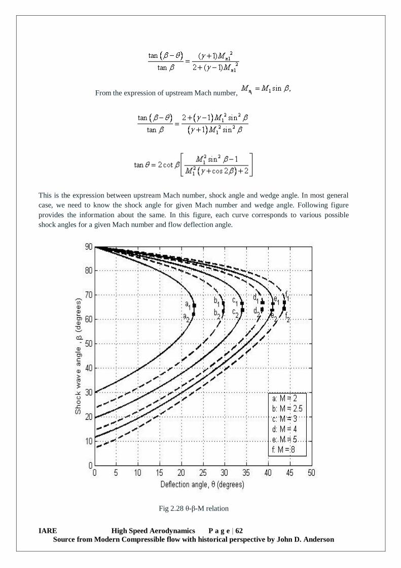
IARE High Speed Aerodynamics P a g e | 62
Source from Modern Compressible flow with historical perspective by John D. Anderson
From the expression of upstream Mach number,
This is the expression between upstream Mach number, shock angle and wedge angle. In most general
case, we need to know the shock angle for given Mach number and wedge angle. Following figure
provides the information about the same. In this figure, each curve corresponds to various possible
shock angles for a given Mach number and flow deflection angle.
Fig 2.28 θ-β-M relation
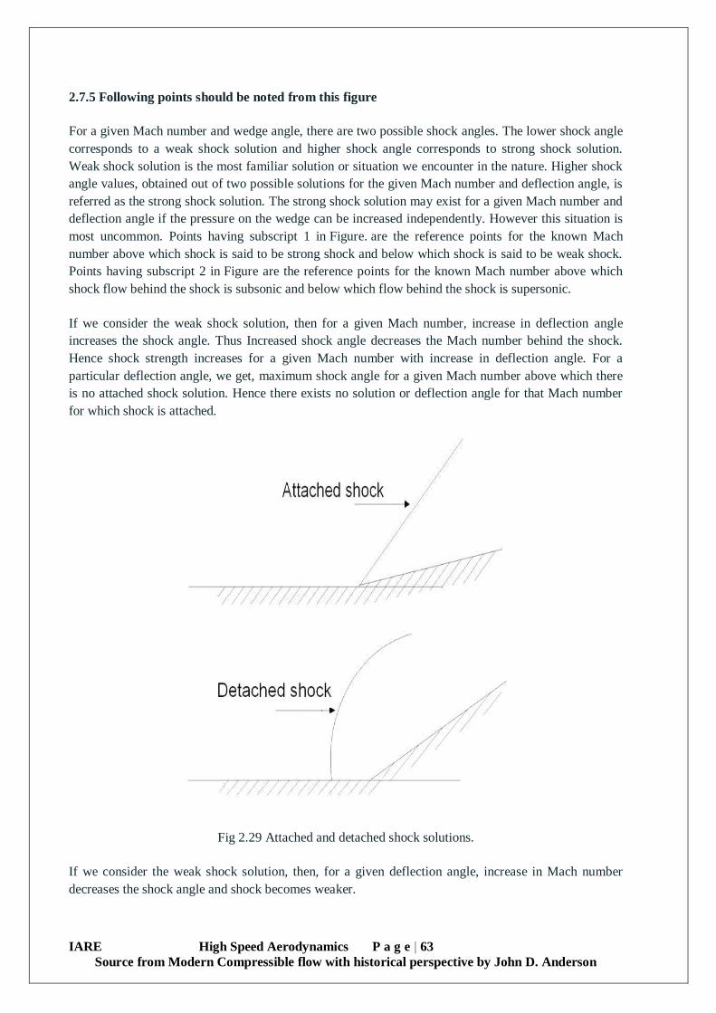
IARE High Speed Aerodynamics P a g e | 63
Source from Modern Compressible flow with historical perspective by John D. Anderson
2.7.5 Following points should be noted from this figure
For a given Mach number and wedge angle, there are two possible shock angles. The lower shock angle
corresponds to a weak shock solution and higher shock angle corresponds to strong shock solution.
Weak shock solution is the most familiar solution or situation we encounter in the nature. Higher shock
angle values, obtained out of two possible solutions for the given Mach number and deflection angle, is
referred as the strong shock solution. The strong shock solution may exist for a given Mach number and
deflection angle if the pressure on the wedge can be increased independently. However this situation is
most uncommon. Points having subscript 1 in Figure. are the reference points for the known Mach
number above which shock is said to be strong shock and below which shock is said to be weak shock.
Points having subscript 2 in Figure are the reference points for the known Mach number above which
shock flow behind the shock is subsonic and below which flow behind the shock is supersonic.
If we consider the weak shock solution, then for a given Mach number, increase in deflection angle
increases the shock angle. Thus Increased shock angle decreases the Mach number behind the shock.
Hence shock strength increases for a given Mach number with increase in deflection angle. For a
particular deflection angle, we get, maximum shock angle for a given Mach number above which there
is no attached shock solution. Hence there exists no solution or deflection angle for that Mach number
for which shock is attached.
Fig 2.29 Attached and detached shock solutions.
If we consider the weak shock solution, then, for a given deflection angle, increase in Mach number
decreases the shock angle and shock becomes weaker.
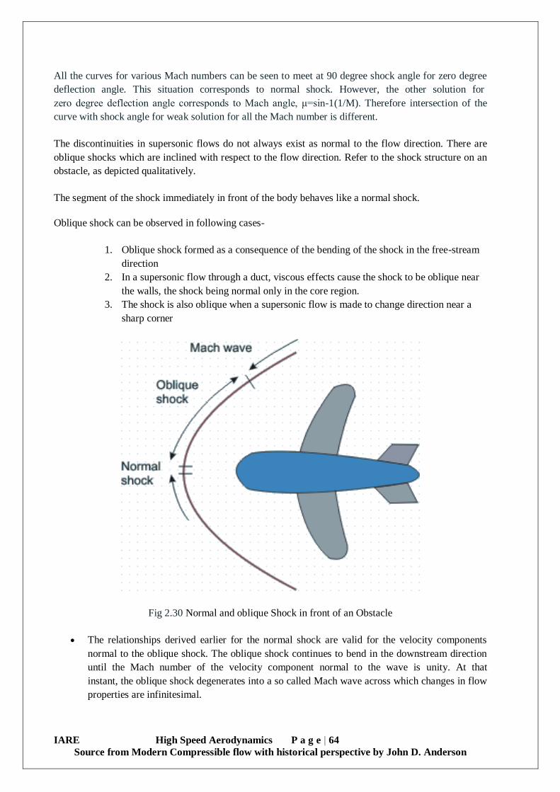
IARE High Speed Aerodynamics P a g e | 64
Source from Modern Compressible flow with historical perspective by John D. Anderson
All the curves for various Mach numbers can be seen to meet at 90 degree shock angle for zero degree
deflection angle. This situation corresponds to normal shock. However, the other solution for
zero degree deflection angle corresponds to Mach angle, μ=sin-1(1/M). Therefore intersection of the
curve with shock angle for weak solution for all the Mach number is different.
The discontinuities in supersonic flows do not always exist as normal to the flow direction. There are
oblique shocks which are inclined with respect to the flow direction. Refer to the shock structure on an
obstacle, as depicted qualitatively.
The segment of the shock immediately in front of the body behaves like a normal shock.
Oblique shock can be observed in following cases-
1. Oblique shock formed as a consequence of the bending of the shock in the free-stream
direction
2. In a supersonic flow through a duct, viscous effects cause the shock to be oblique near
the walls, the shock being normal only in the core region.
3. The shock is also oblique when a supersonic flow is made to change direction near a
sharp corner
Fig 2.30 Normal and oblique Shock in front of an Obstacle
The relationships derived earlier for the normal shock are valid for the velocity components
normal to the oblique shock. The oblique shock continues to bend in the downstream direction
until the Mach number of the velocity component normal to the wave is unity. At that
instant, the oblique shock degenerates into a so called Mach wave across which changes in flow
properties are infinitesimal.
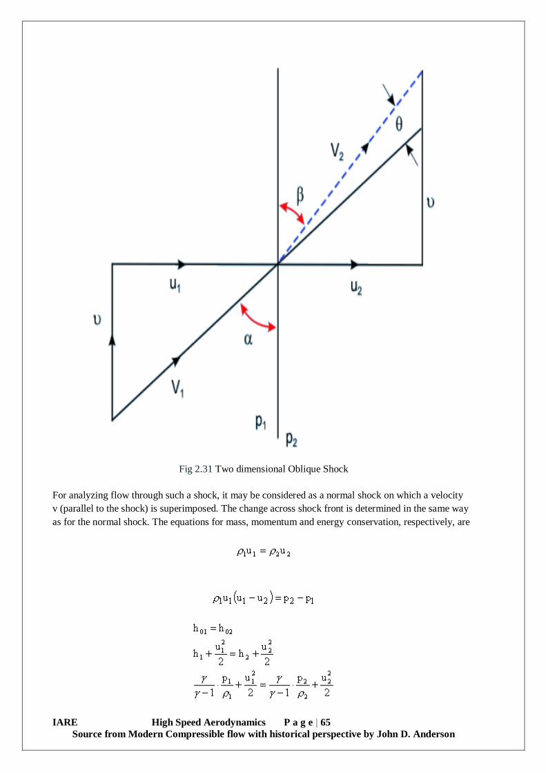
IARE High Speed Aerodynamics P a g e | 65
Source from Modern Compressible flow with historical perspective by John D. Anderson
Fig 2.31 Two dimensional Oblique Shock
For analyzing flow through such a shock, it may be considered as a normal shock on which a velocity
v (parallel to the shock) is superimposed. The change across shock front is determined in the same way
as for the normal shock. The equations for mass, momentum and energy conservation, respectively, are

IARE High Speed Aerodynamics P a g e | 66
Source from Modern Compressible flow with historical perspective by John D. Anderson
These equations are analogous to corresponding equations for normal shock. In addition to these, we
have
And
Modifying normal shock relations by writing and in place of and ,
we obtain
Note that although Ma2sinβ<1, Ma2 might be greater than 1. So the flow behind an oblique shock may
be supersonic although the normal component of velocity is subsonic.
In order to obtain the angle of deflection of flow passing through an oblique shock, we use the relation
Having substituted (tanβ/tanα) from Equation, we get the relation
Sometimes, a design is done in such a way that an oblique shock is allowed instead of a normal
shock. The losses for the case of oblique shock are much less than those of normal shock.This is the
reason for making the nose angle of the fuselage of a supersonic aircraft small.

IARE High Speed Aerodynamics P a g e | 67
Source from Modern Compressible flow with historical perspective by John D. Anderson
2.8 Shock Reflection
Reflection of shock wave from the wall is mainly of two types, regular reflection and irregular or Mach
reflection.
Fig 2.32 Typical regular reflection of shock wave
Fig 2.33 Typical Mach reflection of shock wave
The shock that originates from the corner of the compression wedge makes an angle β with the
freestream velocity vector. Flow behind this shock gets deflected by angle θ and becomes parallel to the
wedge. However, when the shock hits the top wall, the part of the flow which was parallel to the top
wall, upstream of the shock, also gets deflected by angle θ. Hence the flow downstream of the shock
does not remain parallel to the top wall. This contradicts the necessary condition of formation of shock,
hence the primary shock gets reflected from the top wall to cancel out the deflection of the flow and to

IARE High Speed Aerodynamics P a g e | 68
Source from Modern Compressible flow with historical perspective by John D. Anderson
make it parallel to the wall. In this process shock reflection can be observed as the reflection of light
ray, however the incident and reflection angle of shock are dependent on shock upstream Mach number.
Therefore this reflection is called as the regular reflection. Typical pressure deflection diagram for the
streamline ABC.
Fig 2.34 Pressure deflection diagram for the regular reflection case
Providing equal and opposite deflection to the flow as that provided by incident shock is the objective of
reflected shock. However possibility of such a deflection behind the reflected shock depends on the
Mach number behind the incident shock or Mach number upstream to the reflected shock. If the
deflection required is more than the maximum possible deflection for that Mach number then the
reflection of shock does not remain as regular reflection since the reflected shock gets detached from the
wall.
2.8.1 Mach Reflection
Let’s understand the reason for deviation from regular reflection to Mach reflection. We know
from Figure that the presence of reflected shock is mainly to deflect the flow in region B and make it
parallel with the wall. The amount of this flow deflection expected from the reflected shock is same as
that from the primary or incident shock. However, regular reflection ensures that this deflection is less
than the maximum possible defection corresponding to the Mach number in region B in the same figure.
A situation has been shown in Figure which shows the possibility of where the expected deflection
using reflected shock more than the maximum deflection possible corresponding to Mach number in
region B.

IARE High Speed Aerodynamics P a g e | 69
Source from Modern Compressible flow with historical perspective by John D. Anderson
Fig 2.35 Reason for Mach reflection using pressure deflection diagram
Therefore, since reflected shock cannot provide the necessary deflection to the flow so as to make it
parallel to the wall, the incident or primary shock does not reflect like the ray of light or regular
reflection.
2.8.2 Supersonic expansion
Expansion Fan
We have already seen that compression of supersonic flow takes while passing through the shock. In
other words, when the supersonic flow turns into itself then it undergoes the compression through a
shock. Exactly opposite situation can be encountered when the supersonic flow turns out of itself where,
expansion of the supersonic flow takes place. This expansion unlike compression takes place smoothly
through infinite expansion waves hence called as expansion fan. This expansion fan is comprised of
infinite number of expansion waves or Mach waves where every wave is responsible for infinitesimal
amount of deflection. Where supersonic flow turns outward by an angle θ.
Fig 2.36 Schematic of expansion fan

IARE High Speed Aerodynamics P a g e | 70
Source from Modern Compressible flow with historical perspective by John D. Anderson
For better understanding of expansion of supersonic flow, consider that p1, T1 and M1 be the properties
of flow before expansion or upstream of the expansion fan and p2, T2 and M2 be the properties of the
flow after expansion or downstream of the expansion fan due to outward deflection by an angle θ. For
the know upstream flow properties and deflection angle it should be possible for us to calculate the
downstream flow properties. Since the expansion is the continuous and smooth process carried out via
infinite Mach waves, let’s consider one such wave across upstream of which velocity is V and Mach
number is M. Angle made by this Mach wave with the upstream velocity vector is μ. Let’s consider dV
be the change in velocity brought by the Mach wave by turning through an angle dθ. Hence V+dV is
downstream velocity and M+dM is the downstream Mach number. If we construct the velocity triangle
as shown in Figure,then we can use the sin law for triangle as,
Fig 2.37 Velocity triangle across a typical Mach wave during supersonic expansion
But we know that
and
Hence we can re-write Equation as,
We can approximate as
sin dθ ≈ dθ and cos dθ ≈ 1, Therefore Equation can be simplified as,
since dθ tan μ < 1, lets recall the expansion for x<1,

IARE High Speed Aerodynamics P a g e | 71
Source from Modern Compressible flow with historical perspective by John D. Anderson
Neglecting higher order term, we can express Equation as,
But we know that
and hence
Hence above equation becomes,
2.9 PRANDTL-MEYER EXPANSION FLOW
Prandtl Meyer Function
We can see that since for positive value of dθ, we get positive dV which leads to expansion. This
formula is also valid for small angles for compression where we get negative dV. If we integrate this
formula for the total expansion angle then we can get the downstream Mach number.
Before integrating we can express the integrant in Mach number,
V = Ma
ln V = ln M + ln a
We can express here the second term on right hand side in terms of Mach number using the isentropic
relations as,

IARE High Speed Aerodynamics P a g e | 72
Source from Modern Compressible flow with historical perspective by John D. Anderson
Integration of right hand side is as,
Here, v is called as the Prandtl-Meyer function.
θ = v(M2) - v(M1)
Therefore upstream Mach number (M1) we can calculate the upstream Prandtl-Meyer function. Hence
for known flow deflection angle and upstream Mach number we can get the downstream Prandtl-Meyer
function and hence the downstream Mach number.
Process of expansion of supersonic flow is an isentropic process. However, while passing through the
expansion fan, pressure, temperature and density of the flow decreases while Mach number and velocity
increases for the supersonic flow. Moreover, all the total properties remain constant. We can calculate
the total pressure, temperature and density upstream of the expansion using isentropic relations for the
known flow Mach number. From the calculated downstream Mach number, we can calculate all the
static flow properties from known stagnation or total properties.
2.10 Shock Expansion Method for Flow over Airfoil
It is possible to solve many problems in two-dimensional supersonic flow by patching together
appropriate combinations of the oblique shock wave, and the Prandtl-Mayer expansion fan. For
example, let us consider the flow over a simple two-dimensional airfoil section.
Fig2.37: A flat lifting plate. Ma1 is the upstream Mach number, p1 , p2 , et cetera, denote pressures,
and αo is the angle of attack.
IARE High Speed Aerodynamics P a g e | 73
Source from Modern Compressible flow with historical perspective by John D. Anderson
Figure shows a flat plate inclined at an angle of attack, αo, to the oncoming supersonic flow. The
streamline ahead of the leading edge is non-inclined, because there is no upstream influence. Moreover,
the flow streams over the upper and lower surfaces are completely independent of one another. Thus,
the flow on the upper surface is turned through an expansion angle αoby means of a Prandtl-Mayer
expansion fan attached to the leading edge of the airfoil, whereas the flow on the lower side is turned
through a compression angle αo by means of an oblique shock. The flow on the upper surface is
recompressed to the upstream pressure p1 by means of an oblique shock wave attached to the trailing
edge of the airfoil. Likewise, the flow on the lower surface is re-expanded to the upstream pressure by
means of an expansion fan. The uniform pressures,p2 and𝑃2ϒ , respectively, on the upper and lower
surfaces of the airfoil can easily be calculated by means of oblique shock theory and Prandtl-Mayer
expansion theory. Given the pressures, the lift and drag per unit transverse length of the airfoil are
simply
L = (𝑃2′ - P2) c cosα0,
D = (𝑃2′ - P2) c sinα0,
respectively, where c is the chord-length (i.e., width). The increase in entropy of the flow along the
upper surface of the airfoil is not the same as that for the flow along the lower surface, because the
upper and lower shock waves occur at different Mach numbers. Consequently, the streamline attached
to the trailing edge of the airfoil is a slipstream--that is, it separates flows with the same pressures, but
slightly different speeds, temperatures, and densities--inclined at a small angle relative to the free
stream. (The angle of inclination is determined by the requirement that the pressures on both sides of the
slipstream be equal to one another.)
Note that the drag that develops on the airfoil is of a completely different nature to the previously
discussed drags that develop on subsonic airfoils, such as friction drag, form drag, and induced drag.
This new type of drag is termed supersonic wave drag, and exists even in an idealized, inviscid fluid. It
is ultimately due to the trailing shock waves attached to the airfoil.
Comparatively far from the airfoil, the attached shock waves and expansion fans intersect one another.
The expansion fans then attenuate the oblique shocks, making them weak and curved. At very large
distances, the shock waves asymptote to free-stream Mach lines. However, this phenomenon does not
affect the previous calculation of the lift and drag on a flat-plate airfoil.
The Physical Picture of the Flow through a Normal Shock
It is possible to obtain physical picture of the flow through a normal shock by employing some
of the ideas of Fanno line and Rayleigh line Flows. Flow through a normal shock must satisfy
Equations.
Since all the condition of state "1" are known, there is no difficulty in locating state "1" on T-s
diagram. In order to draw a Fanno line curve through state "1", we require a locus of
mathematical states that satisfy Equations. The Fanno line curve does not satisfy Equation.
While Rayleigh line curve through state "1" gives a locus of mathematical states that satisfy
Equations. The Rayleigh line does not satisfy Equation. Both the curves on a same T-s diagram
are shown in Figure.
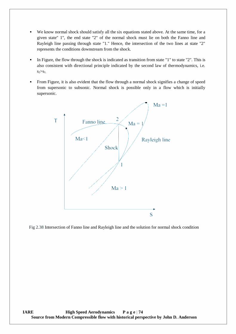
IARE High Speed Aerodynamics P a g e | 74
Source from Modern Compressible flow with historical perspective by John D. Anderson
We know normal shock should satisfy all the six equations stated above. At the same time, for a
given state" 1", the end state "2" of the normal shock must lie on both the Fanno line and
Rayleigh line passing through state "1." Hence, the intersection of the two lines at state "2"
represents the conditions downstream from the shock.
In Figure, the flow through the shock is indicated as transition from state "1" to state "2". This is
also consistent with directional principle indicated by the second law of thermodynamics, i.e.
s2>s1.
From Figure, it is also evident that the flow through a normal shock signifies a change of speed
from supersonic to subsonic. Normal shock is possible only in a flow which is initially
supersonic.
Fig 2.38 Intersection of Fanno line and Rayleigh line and the solution for normal shock condition

IARE High Speed Aerodynamics P a g e | 75
Source from Modern Compressible flow with historical perspective by John D. Anderson
UNIT III
QUASI-ONE DIMENSIONAL FLOWS
3.1 Isentropic flow in nozzles
One and two dimensional compressible flows have already been seen in earlier sections. This section
deals with the quasi-one dimensional flows. For Rayleigh and Fanno flows we had considered the flow
to be one dimensional. The main reason for this assumption is the constancy of the cross sectional area
of duct in the direction of flow. If area of the duct varies in the direction of flow then flow should be
treated as three dimensional flows. However if such a variation is gradual then we can neglect the
changes taking place in cross stream directions. Such flows are called as quasi-one dimensional flows.
Example of a strictly one dimensional and a quasi-one dimensional flow is given in Figure.
Fig 3.1 Control volume for 1D and Quasi 1D flows
Consider a typical control volume shown in Figure. (b) where inlet and outlet properties of the flow are
given by subscripts 1 and 2 respectively.

IARE High Speed Aerodynamics P a g e | 76
Source from Modern Compressible flow with historical perspective by John D. Anderson
3.1.1 Mass conservation equation
The integral form of mass conservation equation is,
For the steady flow, above equation reduces to,
Hence the differential form of mass conservation equation is
3.1.2 Momentum conservation equation
The integral form of momentum conservation equation for inviscid flow is,
For the steady flow this equation transforms to,
Here integration of the pressure is on the stream wise surfaces. This equation is not the usual
algebraicequation. The differential form of this equation can be written as,
Neglecting the higher order terms we get,
We can expand the equation as
multiplying this equation by u we get,
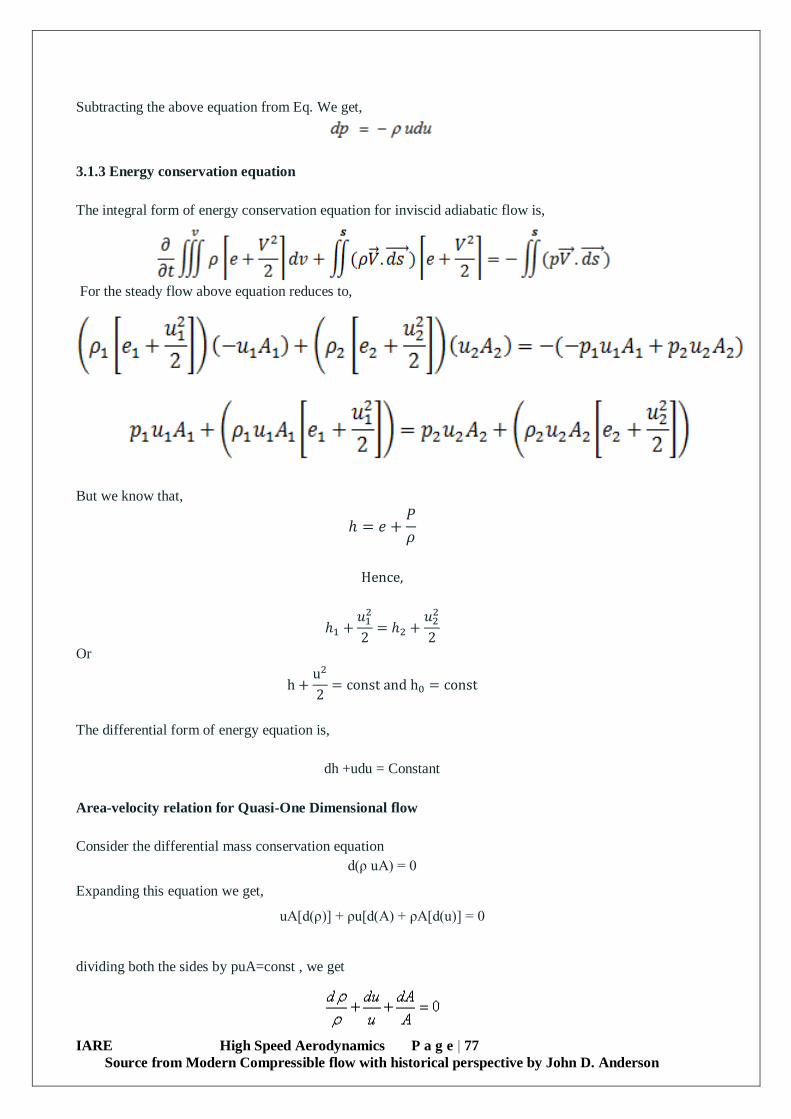
IARE High Speed Aerodynamics P a g e | 77
Source from Modern Compressible flow with historical perspective by John D. Anderson
Subtracting the above equation from Eq. We get,
3.1.3 Energy conservation equation
The integral form of energy conservation equation for inviscid adiabatic flow is,
For the steady flow above equation reduces to,
But we know that,
ℎ = 𝑒 +𝑃
𝜌
Hence,
ℎ1 +𝑢1
2
2= ℎ2 +
𝑢22
2
Or
h +u2
2= const and h0 = const
The differential form of energy equation is,
dh +udu = Constant
Area-velocity relation for Quasi-One Dimensional flow
Consider the differential mass conservation equation
d(ρ uA) = 0
Expanding this equation we get,
uA[d(ρ)] + ρu[d(A) + ρA[d(u)] = 0
dividing both the sides by puA=const , we get

IARE High Speed Aerodynamics P a g e | 78
Source from Modern Compressible flow with historical perspective by John D. Anderson
To obtain the relation between velocity and area we need to replace the term dρ/ρ of above equation.
We know differential form or momentum equation as,
Using the above equation, can be written as,
3.1.4 Many conclusions can be drawn from this equation
1. For positive dA, du will be positive for M>1. Hence for supersonic flows, velocity of the flow
increases with increase in area or divergent portion acts as the nozzle. Similarly, for convergent
portion acts as the diffuser for supersonic flows.
2. For negative dA, du will be positive for M<1. Hence for subsonic flows, velocity of the flow
increases with decrease in area or convergent portion acts as the nozzle. Similarly, for divergent
portion acts as the diffuser for supersonic flows.
3. We can always achieve supersonic flow using a convergent-divergent duct having subsonic
flow at the entry. In such a case, for M=1, we get dA=0, means Mach one will be achieved at
the minimum cross section of the duct. Therefore the minimum cross-section where sonic
conditions are achieved in the convergent divergent duct, is called as throat.
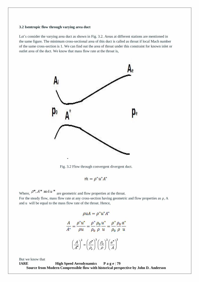
IARE High Speed Aerodynamics P a g e | 79
Source from Modern Compressible flow with historical perspective by John D. Anderson
3.2 Isentropic flow through varying area duct
Let’s consider the varying area duct as shown in Fig. 3.2. Areas at different stations are mentioned in
the same figure. The minimum cross-sectional area of this duct is called as throat if local Mach number
of the same cross-section is 1. We can find out the area of throat under this constraint for known inlet or
outlet area of the duct. We know that mass flow rate at the throat is,
Fig. 3.2 Flow through convergent divergent duct.
Where, are geometric and flow properties at the throat.
For the steady flow, mass flow rate at any cross-section having geometric and flow properties as ρ, A
and u will be equal to the mass flow rate of the throat. Hence,
But we know that
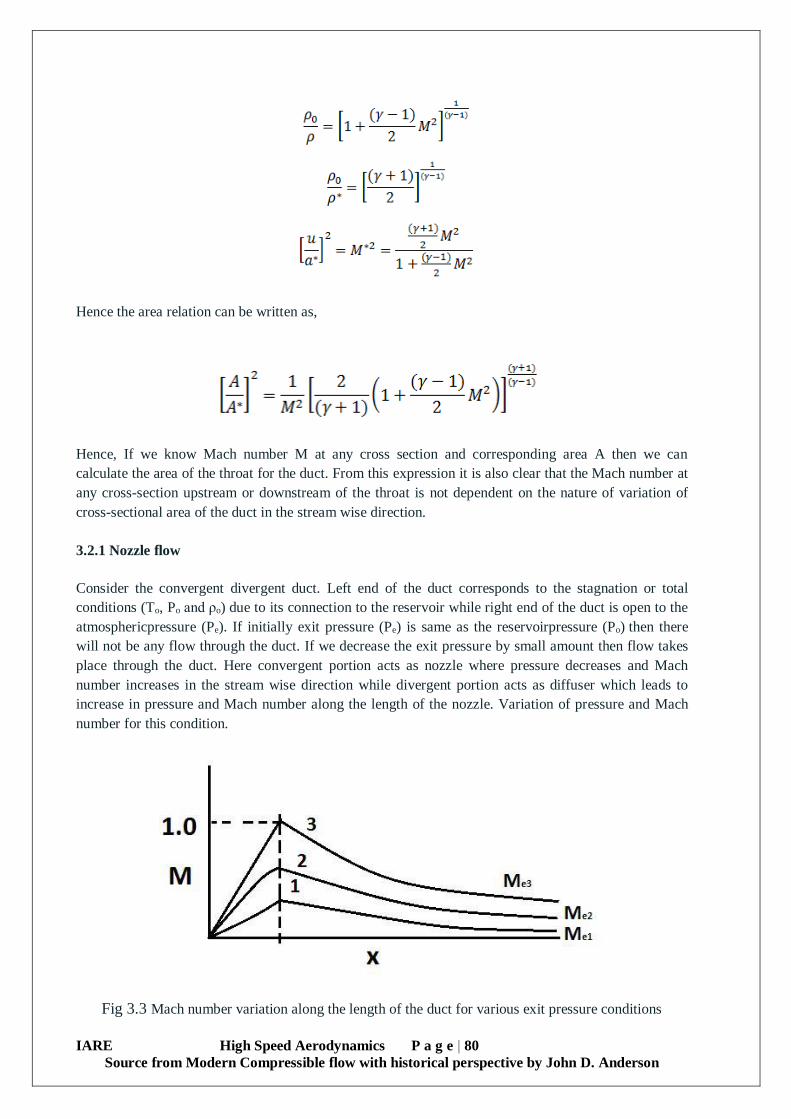
IARE High Speed Aerodynamics P a g e | 80
Source from Modern Compressible flow with historical perspective by John D. Anderson
Hence the area relation can be written as,
Hence, If we know Mach number M at any cross section and corresponding area A then we can
calculate the area of the throat for the duct. From this expression it is also clear that the Mach number at
any cross-section upstream or downstream of the throat is not dependent on the nature of variation of
cross-sectional area of the duct in the stream wise direction.
3.2.1 Nozzle flow
Consider the convergent divergent duct. Left end of the duct corresponds to the stagnation or total
conditions (To, Po and ρo) due to its connection to the reservoir while right end of the duct is open to the
atmosphericpressure (Pe). If initially exit pressure (Pe) is same as the reservoirpressure (Po) then there
will not be any flow through the duct. If we decrease the exit pressure by small amount then flow takes
place through the duct. Here convergent portion acts as nozzle where pressure decreases and Mach
number increases in the stream wise direction while divergent portion acts as diffuser which leads to
increase in pressure and Mach number along the length of the nozzle. Variation of pressure and Mach
number for this condition.
Fig 3.3 Mach number variation along the length of the duct for various exit pressure conditions

IARE High Speed Aerodynamics P a g e | 81
Source from Modern Compressible flow with historical perspective by John D. Anderson
Fig 3.4 Pressure variation along the length of the duct for various exit pressure conditions
Further decrease in pressure at the exit of the duct shifts the pressure and Mach number curves as shown
in Figure tagged by 2. Mass flow continues to increase with decreasing the exit pressure from conditions
from 1 to 2. Condition 3 in this figure represents first critical condition or a particular value of exit
pressure at which Mach number at the minimum cross-section of the duct becomes 1 or sonic.
From Figure a it is clear that convergent portion continues to act as nozzle while divergent portion acts
as diffuser. Pressure at the throat where Mach number has reached 1 attains the reference star value
which is equal to 0.528 times the reservoir pressure for isentropic air flow. Further decrease in exit
pressure beyond the first critical pressure (corresponding to situation 3), does not change the role of
convergent portion as the nozzle. The pressure and Mach number in the convergent portion also remain
unchanged with further decrease in exit pressure. Once the sonic state is achieved at the minimum cross
section, mass flow rate through the duct attains saturation. Hence duct or the nozzle is said to be choked
for any pressure value lower than the first critical condition. Typical mass flow rate variation for air
flow with change in exit pressure is shown in Figure.
Fig 3.5 Variation of mass flow rate for air with change in exit pressure
Variation of pressure and Mach number for a typical exit pressure just below first critical conditions is
shown in Figure a and b respectively. As discussed earlier, for this situation also pressure decreases and
Mach number increases in the convergent portion of the duct. Thus Mach number attains value 1 at the
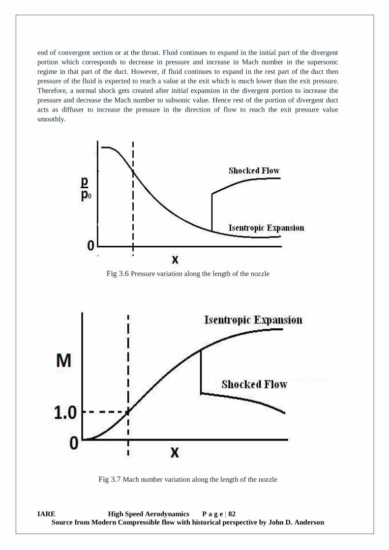
IARE High Speed Aerodynamics P a g e | 82
Source from Modern Compressible flow with historical perspective by John D. Anderson
end of convergent section or at the throat. Fluid continues to expand in the initial part of the divergent
portion which corresponds to decrease in pressure and increase in Mach number in the supersonic
regime in that part of the duct. However, if fluid continues to expand in the rest part of the duct then
pressure of the fluid is expected to reach a value at the exit which is much lower than the exit pressure.
Therefore, a normal shock gets created after initial expansion in the divergent portion to increase the
pressure and decrease the Mach number to subsonic value. Hence rest of the portion of divergent duct
acts as diffuser to increase the pressure in the direction of flow to reach the exit pressure value
smoothly.
Fig 3.6 Pressure variation along the length of the nozzle
Fig 3.7 Mach number variation along the length of the nozzle
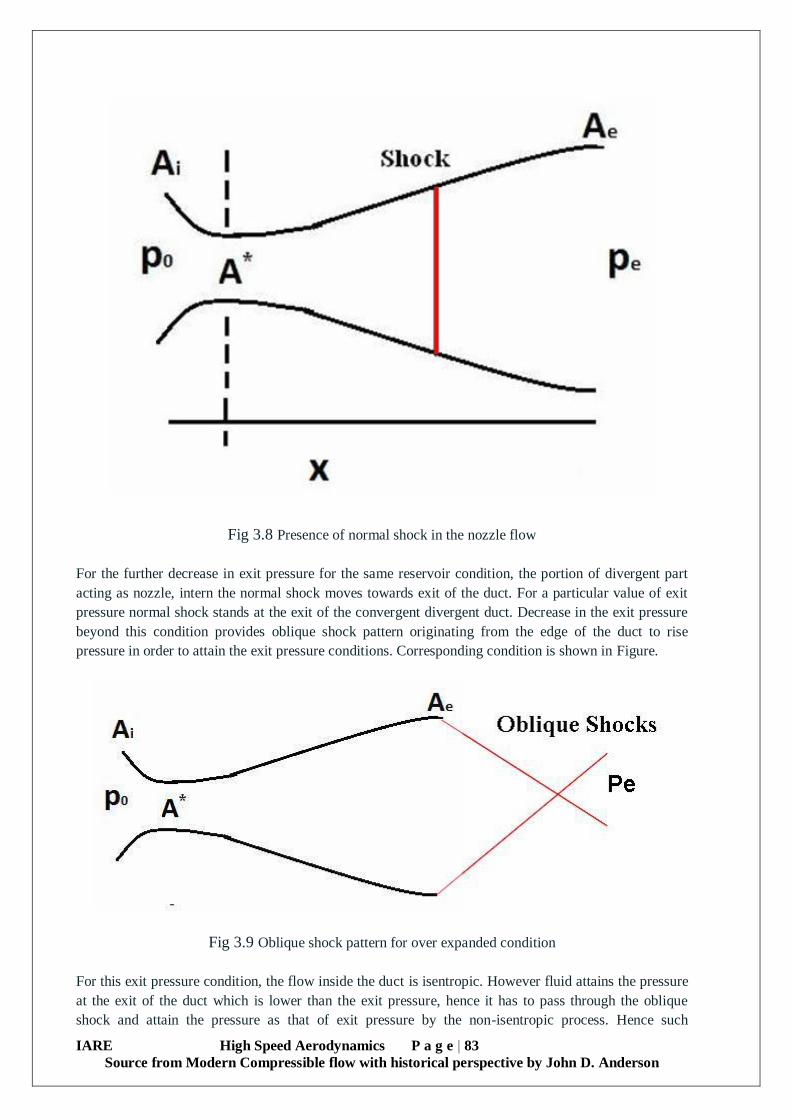
IARE High Speed Aerodynamics P a g e | 83
Source from Modern Compressible flow with historical perspective by John D. Anderson
Fig 3.8 Presence of normal shock in the nozzle flow
For the further decrease in exit pressure for the same reservoir condition, the portion of divergent part
acting as nozzle, intern the normal shock moves towards exit of the duct. For a particular value of exit
pressure normal shock stands at the exit of the convergent divergent duct. Decrease in the exit pressure
beyond this condition provides oblique shock pattern originating from the edge of the duct to rise
pressure in order to attain the exit pressure conditions. Corresponding condition is shown in Figure.
Fig 3.9 Oblique shock pattern for over expanded condition
For this exit pressure condition, the flow inside the duct is isentropic. However fluid attains the pressure
at the exit of the duct which is lower than the exit pressure, hence it has to pass through the oblique
shock and attain the pressure as that of exit pressure by the non-isentropic process. Hence such

IARE High Speed Aerodynamics P a g e | 84
Source from Modern Compressible flow with historical perspective by John D. Anderson
condition of the duct is called as over expanded nozzle' and it is shown in Figure. Decrease in exit
pressure beyond this over expanded condition, decreases the strength of oblique shock and hence the
amount of pressure rise. Hence at a particular value of exit pressure fluid pressure at the exit of the duct
becomes exactly equal to the exit pressure and flow becomes completely isentropic for the duct. In this
condition both convergent and divergent portions of the duct act as nozzle to expand the flow smoothly,
hence duct is called as convergent divergent nozzle. Expansion of the flow in the convergent divergent
nozzle is mentioned as 'isentropic expansion' in Figures a and b. Further decrease in exit pressure
beyond the isentropic condition corresponds to more fluid pressure at the exit in comparison with the
ambient pressure. Hence expansion fan gets originated from the edge of the nozzle to decrease the
pressure smoothly to reach the ambient condition isentropically. Nozzle flow for such a situation is
termed as 'under expanded nozzle flow'. Corresponding flow pattern is shown in Figure.
Fig 3.10 Expansion fan pattern for under expanded condition
3.4 Choked Flow
Choked flow is a compressible flow effect. The parameter that becomes "choked" or "limited" is the
fluid velocity. Choked flow is a fluid dynamic condition associated with the Venturi effect. When a
flowing fluid at a given pressure and temperature passes through a restriction (such as the throat of a
convergent-divergent nozzle or a valve in a pipe) into a lower pressure environment the fluid velocity
increases. At initially subsonic upstream conditions, the conservation of mass principle requires the
fluid velocity to increase as it flows through the smaller cross-sectional area of the restriction. At the
same time, the Venturi effect causes the static pressure, and therefore the density, to decrease
downstream beyond the restriction. Choked flow is a limiting condition where the mass flow rate will
not increase with a further decrease in the downstream pressure environment while upstream pressure is
fixed.
For homogeneous fluids, the physical point at which the choking occurs for adiabatic conditions is
when the exit plane velocity is at sonic conditions i.e. at a Mach number of 1. At choked flow, the mass
flow rate can be increased only by increasing density upstream and at the choke point.
The choked flow of gases is useful in many engineering applications because the mass flow rate is
independent of the downstream pressure, and depends only on the temperature and pressure
andhencethedensityofthegasontheupstreamsideoftherestriction.Underchokedconditions, valves and
calibrated orifice plates can be used to produce a desired mass flowrate.

IARE High Speed Aerodynamics P a g e | 85
Source from Modern Compressible flow with historical perspective by John D. Anderson
3.4.1 Chocked mass flow rate of the nozzle
We have already seen in Figure, that mass flow rate of the nozzle remains unaltered after flow gets
chocked. This chocked mass flow rate can be calculated as,
But we know that,
Hence
However,
Hence
From this expression it is clear that for a convergent divergent nozzle, for given throat area, choked
mass flow rate remains constant for the fixed reservoir (P0 and T0) conditions. Therefore choked mass
flow rate can be increased by increasing the reservoir pressure P0 or decreasing reservoir temperature
T0.
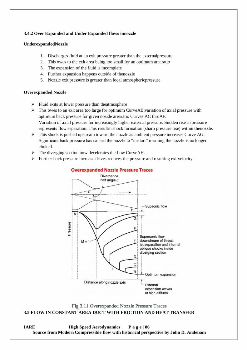
IARE High Speed Aerodynamics P a g e | 86
Source from Modern Compressible flow with historical perspective by John D. Anderson
3.4.2 Over Expanded and Under Expanded flows innozzle
UnderexpandedNozzle
1. Discharges fluid at an exit pressure greater than the externalpressure
2. This owes to the exit area being too small for an optimum arearatio
3. The expansion of the fluid is incomplete
4. Further expansion happens outside of thenozzle
5. Nozzle exit pressure is greater than local atmosphericpressure
Overexpanded Nozzle
Fluid exits at lower pressure than theatmosphere
This owes to an exit area too large for optimum CurveAB:variation of axial pressure with
optimum back pressure for given nozzle arearatio Curves AC thruAF:
Variation of axial pressure for increasingly higher external pressure. Sudden rise in pressure
represents flow separation. This resultin shock formation (sharp pressure rise) within thenozzle.
This shock is pushed upstream toward the nozzle as ambient pressure increases Curve AG:
Significant back pressure has caused the nozzle to “unstart” meaning the nozzle is no longer
choked.
The diverging section now decelerates the flow CurveAH.
Further back pressure increase drives reduces the pressure and resulting exitvelocity
Fig 3.11 Overexpanded Nozzle Pressure Traces
3.5 FLOW IN CONSTANT AREA DUCT WITH FRICTION AND HEAT TRANSFER

IARE High Speed Aerodynamics P a g e | 87
Source from Modern Compressible flow with historical perspective by John D. Anderson
3.5.1 Flow with friction
Consider a flow through constant area pipe as shown in Figure. A subsonic or supersonic flow enters in
the pipe at section 1 and leaves at section 2. Thermodynamic properties along with the velocity of the
flow change from their initial value at station 1 to the station 2 in the presence of friction force. This 1D
flow with friction is called as Fanno flow. Analysis of this flow would lead to prediction of properties of
the flow at the exit for known inletconditions and pipe configuration.
.
Fig 3.12 Flow through constant area pipe
Here we will be considering the effect of friction between pipe wall and fluid. However this assumption
will be used only in momentum equation. Hence total temperature can be considered to be constant in
the flow process. The 1D governing equations for this flow are,
ρ1u1 = ρ2u2(mass conservation)
And
(energy conservation)
The main change takes place in momentum equation. Therefore consider the integral form of
momentum equation for 1D flow.
Let’s assume the flow to be steady through the pipe. Hence,
for integration of pressure and momentum terms, area is the cross sectional area while for the shear
stress term areas the circumferential area of the pipe. Therefore the wetted area for shear stress includes
diameter and length of the pipe. Negative sign should be associated with the shear stress term since
shear acts in the direction opposite to the flow. Hence the momentum equation is,

IARE High Speed Aerodynamics P a g e | 88
Source from Modern Compressible flow with historical perspective by John D. Anderson
p1 + ρu12 = p1 + ρu1
2 + F
where term F corresponds the frictional force and can be expressed in terms of pipe dimensions and
friction coefficient.
Let’s try to express the change in static and total properties of the flow from station 1 and 2 of the pipe
due to consideration of wall shear or friction.
Since total temperature is constant, we can express the static temperature ratio as
Hence,
From, mass conservation equation, we can get,
ρ1u1 = ρ2u2
But,
Substituting this expression in mass conservation equation, we get,
We can use ideal gas equation to calculate the density ratio from pressure and temperature ratio.

IARE High Speed Aerodynamics P a g e | 89
Source from Modern Compressible flow with historical perspective by John D. Anderson
The earlier equation are for static property ratios. For total property ratios between two stations we
have,
These expressions provide the ratios of thermodynamic properties for the known Mach number at
station 1 and 2.
3.5.2 Reference conditions for Fanno flow
If the inlet flow, either subsonic or supersonic, attains Mach number equal to 1 or sonic condition, at the
station 2, then such a condition is taken as reference for calculations of Fanno flow. The corresponding
length of the pipe is terms as critical length of the pipe. We can use the reference conditions for
frictional pipe flow analysis. The expressions for property ratios are then given as,

IARE High Speed Aerodynamics P a g e | 90
Source from Modern Compressible flow with historical perspective by John D. Anderson
Since M2 is equal to 1, the Mach number at station 1 (M1) is the freestream Mach number (M∞).
3.5.3 Differential relations and analysis of flow with friction,
We know the mass, momentum and energy equations for 1D flow with friction. Herewith we will try to
derive the differential form for the same.
mass conservation
Differential form of conservation equation
Energy equation
Differential form of energy equation
For momentum equation, consider the control volume shown in Fig. 2.1 and initially consider the steady
integral form of the momentum equation
We know that, for integration of wall shear, the area of to be considered is the circumferential area. For
integration of pressure and momentum term, the area of to be considered is cross-sectional area, ,
hence

IARE High Speed Aerodynamics P a g e | 91
Source from Modern Compressible flow with historical perspective by John D. Anderson
If we consider the distance between two stations to be infinitesimal (dx) Hence the differential form of
the momentum equation is as,
We can use the mass conservation equation and simplify the above equation,
Using above equation, the equation can be simplified as,
As we know,
Using this equation we can re-write the Equation as,
We can use the definition of skin friction coefficient as,

IARE High Speed Aerodynamics P a g e | 92
Source from Modern Compressible flow with historical perspective by John D. Anderson
Hence differential form of momentum equation becomes,
From further simplification, we can replace the dynamic pressure, as,
Hence,
Above equation represents the differential form of momentum equation.
We can use the Equation for further analysis of Fanno flow. For this purpose lets replace dp/p and du/u
of this equation. We can use ideal gas equation for replacing dp/p as,
(Differential form of ideal gas equation)
using mass differential form of mass conservation equation, we get,
(Modified differential form of ideal gas equation)
For this purpose let’s re-express the terms du/u and dT/T.
As we know
But

IARE High Speed Aerodynamics P a g e | 93
Source from Modern Compressible flow with historical perspective by John D. Anderson
We can use this equation for replacing the term du/u of Equation. However we can further simplify this
equation by replacing dT/T. As,
Dividing by M(γRT)0.5 both the sides
We can use the Equation to replace the term dT/T
This is the simplest form of du/u term expressed in terms of Mach number and specific heat ratio.

IARE High Speed Aerodynamics P a g e | 94
Source from Modern Compressible flow with historical perspective by John D. Anderson
3.5.4 Analysis of Fanno Flow
We can use the Equation for critical analysis of Fanno flow. For this purpose let’s replace dp/p and du/u
of this equation.
Let again consider Equation again and replace the term du/u, we get,
Modified differential form of ideal gas equation can be re-written using equation as
Now let’s consider the differential form of momentum Equation and replace the term du/u and dp/p
using Equation, we get,

IARE High Speed Aerodynamics P a g e | 95
Source from Modern Compressible flow with historical perspective by John D. Anderson
We can clearly observe that𝑑𝑀
𝑑𝑥> 0 if M<1 and
𝑑𝑀
𝑑𝑥< 0 for M>1.
Hence from Equation, we can clearly state that, for subsonic flow Mach number increases in the
presence of friction, while Mach number for supersonic flow decreases in the presence of friction.
From Equation, it becomes clear that, for increases in Mach number, velocity of the subsonic flow
increases while that of supersonic flow decreases due to decrease in Mach number. From Equation, it
becomes clear that temperature of the subsonic flow decreases due to increase in Mach number in the
presence of friction while temperature increases for supersonic flow with friction. We can prove
from Equation that pressure decreases for subsonic flow while pressure increases for supersonic flow
with friction. For entropy change we can arrive at the expression as,
Tds = dh – vdp
For supersonic flow dM is negative however 1 - M2 is also negative, therefore ds is positive for
supersonic flow. For subsonic flow dM is positive however 1 - M2 is also positive, therefore ds is
positive for supersonic flow. This expression clearly proves that entropy increases for both subsonic and
supersonic flows while sonic flow is isentropic.
3.6 Fanno line or curve
Typical Fanno line for a particular mass flow rate is shown in Fig. 3.13. Previously proved facts are
clearly evident in this figure. For a subsonic flow through a frictional pipe, enthalpy decreases and
entropy increases. With increase in length of pipe, more expansion of the flow takes place for the
subsonic flow due to increase in Mach number, decrease in pressure and increase in velocity. For a
particular length of pipe flow, inlet subsonic flow attains sonic state at the exit. Corresponding length of
the pipe is called as critical length. Further increase in length of pipe doesn’t change state at the exit
however inlet conditions change and subsonic flow becomes lower subsonic. Hence the flow condition
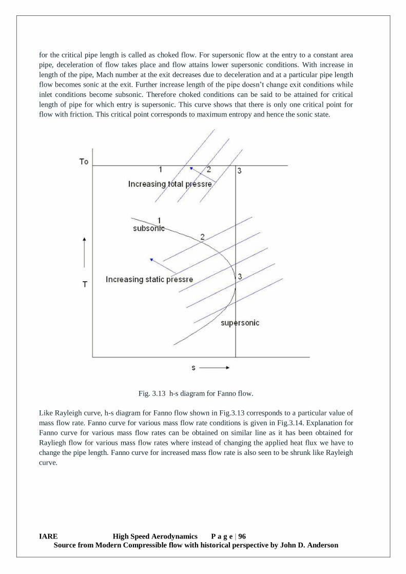
IARE High Speed Aerodynamics P a g e | 96
Source from Modern Compressible flow with historical perspective by John D. Anderson
for the critical pipe length is called as choked flow. For supersonic flow at the entry to a constant area
pipe, deceleration of flow takes place and flow attains lower supersonic conditions. With increase in
length of the pipe, Mach number at the exit decreases due to deceleration and at a particular pipe length
flow becomes sonic at the exit. Further increase length of the pipe doesn’t change exit conditions while
inlet conditions become subsonic. Therefore choked conditions can be said to be attained for critical
length of pipe for which entry is supersonic. This curve shows that there is only one critical point for
flow with friction. This critical point corresponds to maximum entropy and hence the sonic state.
Fig. 3.13 h-s diagram for Fanno flow.
Like Rayleigh curve, h-s diagram for Fanno flow shown in Fig.3.13 corresponds to a particular value of
mass flow rate. Fanno curve for various mass flow rate conditions is given in Fig.3.14. Explanation for
Fanno curve for various mass flow rates can be obtained on similar line as it has been obtained for
Rayliegh flow for various mass flow rates where instead of changing the applied heat flux we have to
change the pipe length. Fanno curve for increased mass flow rate is also seen to be shrunk like Rayleigh
curve.
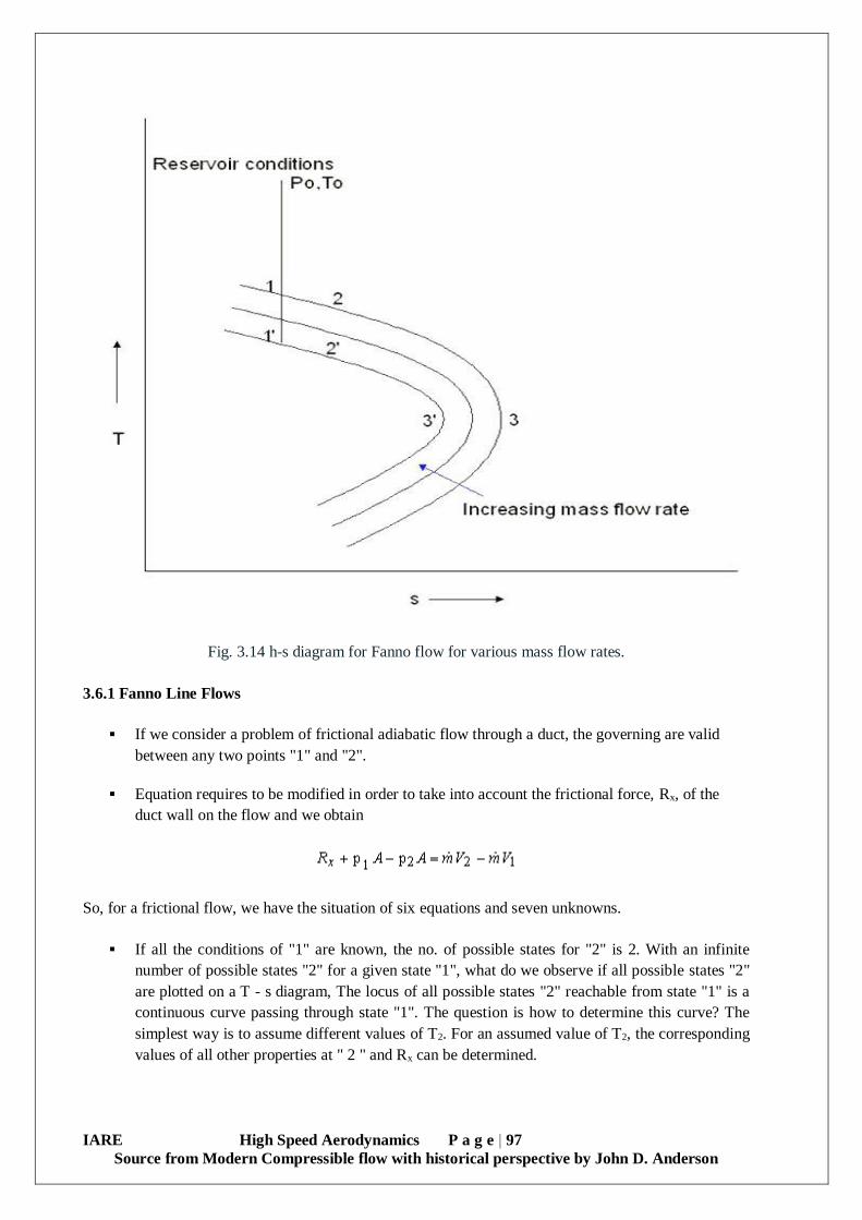
IARE High Speed Aerodynamics P a g e | 97
Source from Modern Compressible flow with historical perspective by John D. Anderson
Fig. 3.14 h-s diagram for Fanno flow for various mass flow rates.
3.6.1 Fanno Line Flows
If we consider a problem of frictional adiabatic flow through a duct, the governing are valid
between any two points "1" and "2".
Equation requires to be modified in order to take into account the frictional force, Rx, of the
duct wall on the flow and we obtain
So, for a frictional flow, we have the situation of six equations and seven unknowns.
If all the conditions of "1" are known, the no. of possible states for "2" is 2. With an infinite
number of possible states "2" for a given state "1", what do we observe if all possible states "2"
are plotted on a T - s diagram, The locus of all possible states "2" reachable from state "1" is a
continuous curve passing through state "1". The question is how to determine this curve? The
simplest way is to assume different values of T2. For an assumed value of T2, the corresponding
values of all other properties at " 2 " and Rx can be determined.
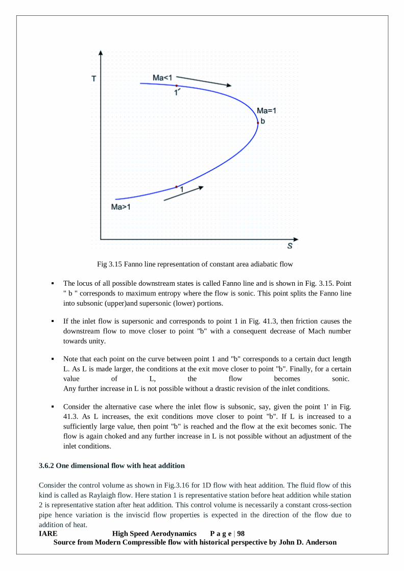
IARE High Speed Aerodynamics P a g e | 98
Source from Modern Compressible flow with historical perspective by John D. Anderson
Fig 3.15 Fanno line representation of constant area adiabatic flow
The locus of all possible downstream states is called Fanno line and is shown in Fig. 3.15. Point
" b " corresponds to maximum entropy where the flow is sonic. This point splits the Fanno line
into subsonic (upper)and supersonic (lower) portions.
If the inlet flow is supersonic and corresponds to point 1 in Fig. 41.3, then friction causes the
downstream flow to move closer to point "b" with a consequent decrease of Mach number
towards unity.
Note that each point on the curve between point 1 and "b" corresponds to a certain duct length
L. As L is made larger, the conditions at the exit move closer to point "b". Finally, for a certain
value of L, the flow becomes sonic.
Any further increase in L is not possible without a drastic revision of the inlet conditions.
Consider the alternative case where the inlet flow is subsonic, say, given the point 1' in Fig.
41.3. As L increases, the exit conditions move closer to point "b". If L is increased to a
sufficiently large value, then point "b" is reached and the flow at the exit becomes sonic. The
flow is again choked and any further increase in L is not possible without an adjustment of the
inlet conditions.
3.6.2 One dimensional flow with heat addition
Consider the control volume as shown in Fig.3.16 for 1D flow with heat addition. The fluid flow of this
kind is called as Raylaigh flow. Here station 1 is representative station before heat addition while station
2 is representative station after heat addition. This control volume is necessarily a constant cross-section
pipe hence variation is the inviscid flow properties is expected in the direction of the flow due to
addition of heat.

IARE High Speed Aerodynamics P a g e | 99
Source from Modern Compressible flow with historical perspective by John D. Anderson
Fig.3.16: Typical Control volume for 1D flow with heat addition.
Assume the flow to be inviscid and steady between these two stations. Therefore the mass and
momentum conservation equations remain unaltered from the normal shock case but energy equation
will have a term corresponding to external heat addition in comparison with equation. Hence the 1D
conservation equations for flow with heat addition are as follows.
Here ‘q’ is amount of heat added per unit mass. Hence,
However, we know that
q = ho2 - ho1 = cp(To2 - To1)
This equation suggests that change in total temperature takes place due to heat addition between two
stations.
Let’s represent the ratios of static and total properties in terms of upstream (station 1) and downstream
(station 2) Mach number and specific heat ratio. Let’s consider the momentum equation,

IARE High Speed Aerodynamics P a g e | 100
Source from Modern Compressible flow with historical perspective by John D. Anderson
Also from ideal gas assumption
But
ρ1u1 = ρ2u2
,
Therefore,
Hence from Eq. we get,
Therefore,
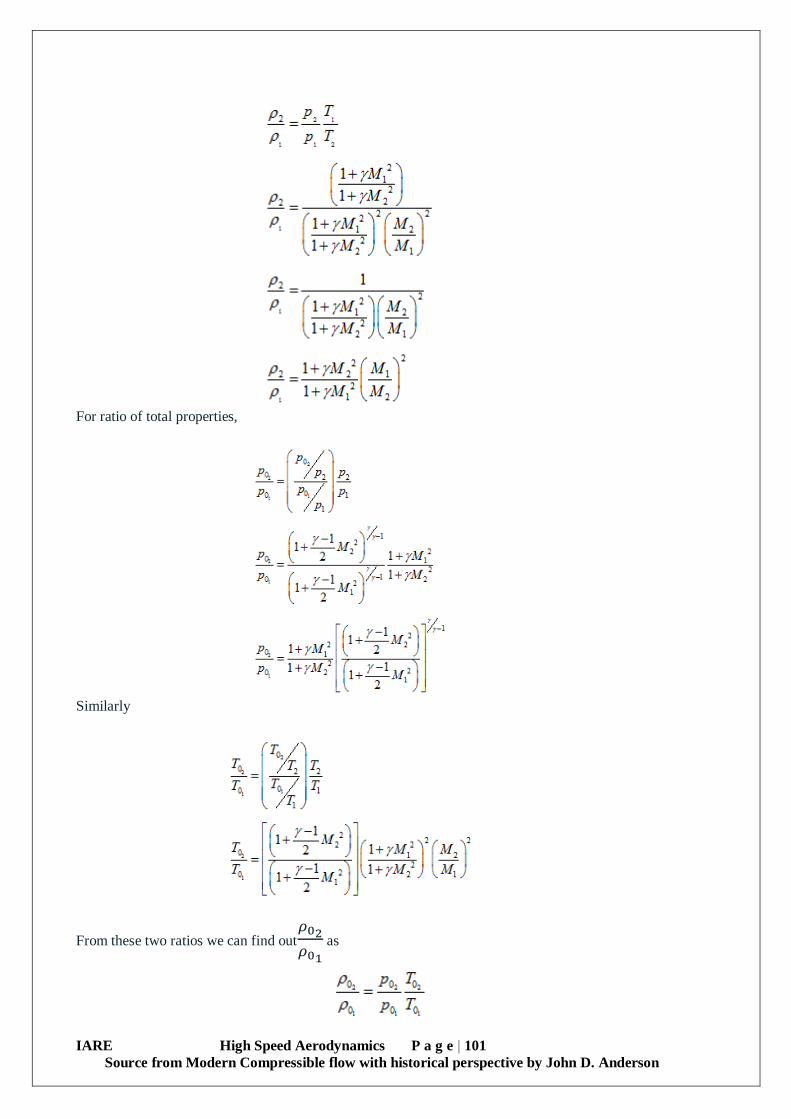
IARE High Speed Aerodynamics P a g e | 101
Source from Modern Compressible flow with historical perspective by John D. Anderson
For ratio of total properties,
Similarly
From these two ratios we can find out𝜌02
𝜌01
as

IARE High Speed Aerodynamics P a g e | 102
Source from Modern Compressible flow with historical perspective by John D. Anderson
3.6.3 Reference conditions for flows with heat addition
We have represented all the ratios in terms of upstream and downstream Mach numbers. If we consider
a particular case where heat addition leads to downstream Mach number equal to one or post heat
addition Mach number is unity, then equations can be written as,
Since M2 = 1 & p2 = p* & p1 = p∞ & M1 = M∞. Here flow properties after heat addition are the stared
quantities due to unity of the local Mach number. Hence these quantities are of very much of
importance since can be used as reference quantities.
Similarly
From all the ratios for 1D flow with heat addition, following conclusions can be drawn for supersonic
and subsonic flows.

IARE High Speed Aerodynamics P a g e | 103
Source from Modern Compressible flow with historical perspective by John D. Anderson
1. Addition of heat in supersonic flows
Decreases Mach number
Increases static pressure
Increases static temperature
Decreases total pressure
Increases total temperature
Decreases velocity
2. Addition of heat in subsonic flow
Increases Mach number
Decreases static pressure
Increases static temperature if𝑀∞ < 𝛾−1/2 and decreases if𝑀∞ > 𝛾−1/2
Decreases total pressure
Increases total temperature
Increases velocity
Hence supersonic flow decelerates towards sonic value while subsonic flow accelerates towards the
same due to heat addition. In a way, having a subsonic flow to start with we can keep on adding heat to
reach sonic and then remove heat to attain required supersonic flow conditions. Exactly reverse
procedure needs to be followed if givenflow is supersonic and the target is to attain specified subsonic
condition.
It had been shown that addition of heat in subsonic flow increases the static temperature till𝑀∞ <
𝛾−1/2 and decreases afterwards. Main reason for this phenomenon is explained herewith. Addition of
heat to subsonic flow increases the velocity and temperature initially for small amount of heat addition.
Therefore both Kinetic energy (KE) and Internal energy (IE) of the flow increase due to externally
added heat in subsonic flow. However for a given mass flow rate, rate of increase of KE is more than IE
for given amount of heat addition. Therefore after particular amount of addition of external heat, it
becomes impossible to increase IE (hence temperature) and KE (hence velocity) both keeping mass
flow rate same. As a result beyond particular amount of heat addition for a given mass flow rate
condition, temperature (hence IE) decreases but velocity (hence KE) continues to increase. We can as
well interpreted the same phenomenon as, after certain critical amount of heat addition in subsonic flow
added external heat becomes insufficient to increase the velocity (hence KE) while keeping the mass
flow rate same, hence required extra energy is supplied by the flow itself from its internal energy, by
virtue of which temperature decrease though we add heat in subsonic flow.
From the above mentioned formulae for sonic conditions or ‘star’ properties, we can calculate total
temperature of the sonic flow after heat addition from any given initial conditions and hence the amount
of heat required to be added to reach sonic condition from any given initial conditions. The properties at
this sonic conditions for a given mass flow rate remain independent of upstream or freestream Mach
number. Therefore, we can use this concept or these properties as reference properties for handling 1D
flows with heat addition.

IARE High Speed Aerodynamics P a g e | 104
Source from Modern Compressible flow with historical perspective by John D. Anderson
If the amount of heat added in the flow is more than the critical heat required to reach sonic condition,
then flow cannot accommodate this heat. The main reason for this fact is the anchoring of conditions
after heat addition to sonic point. Hence to accommodate the added extra heat, upstream conditions of
the flow change from supersonic to subsonic or from subsonic to lower subsonic for which the
externally added heat is the heat required to reach sonic condition.
3.7 Rayleigh curve
As we know, Rayleigh flow is called as the flow with heat addition. The curve or plot or state chart
dealing with heat addition is called Rayleigh curve. Let’s derive the expression for this curve in p-v and
h-s chart.
Mass Conservation
Momentum Conservation
For 1D, it can be expressed as pA + ρv2A = const, called as Impulse function or Thrust function.
Energy Conservation
We can draw a p-v diagram for flow with heat addition or Rayleigh flow like Hugoniot curve, using
momentum equation as,
This equation is the equation for straight line on p-v diagram where k2 corresponds to slope which
eventually is the mass flow rate. Hence, slope of the line joining any point, corresponding to initial state
and final state on Rayleigh curve, represents mass fluxes or mass flow rates. This fact is same as that
observed for Hugoniot curve.
Slope of this Rayleigh line can be calculated as
p1 + v1k2 = p2 + v2k
2
Such curve represented by points 1, 2, 3 and 4 for flow with heat addition is as shown in Figure
3.16 along with the isentropic and isothermal line on p-v chart
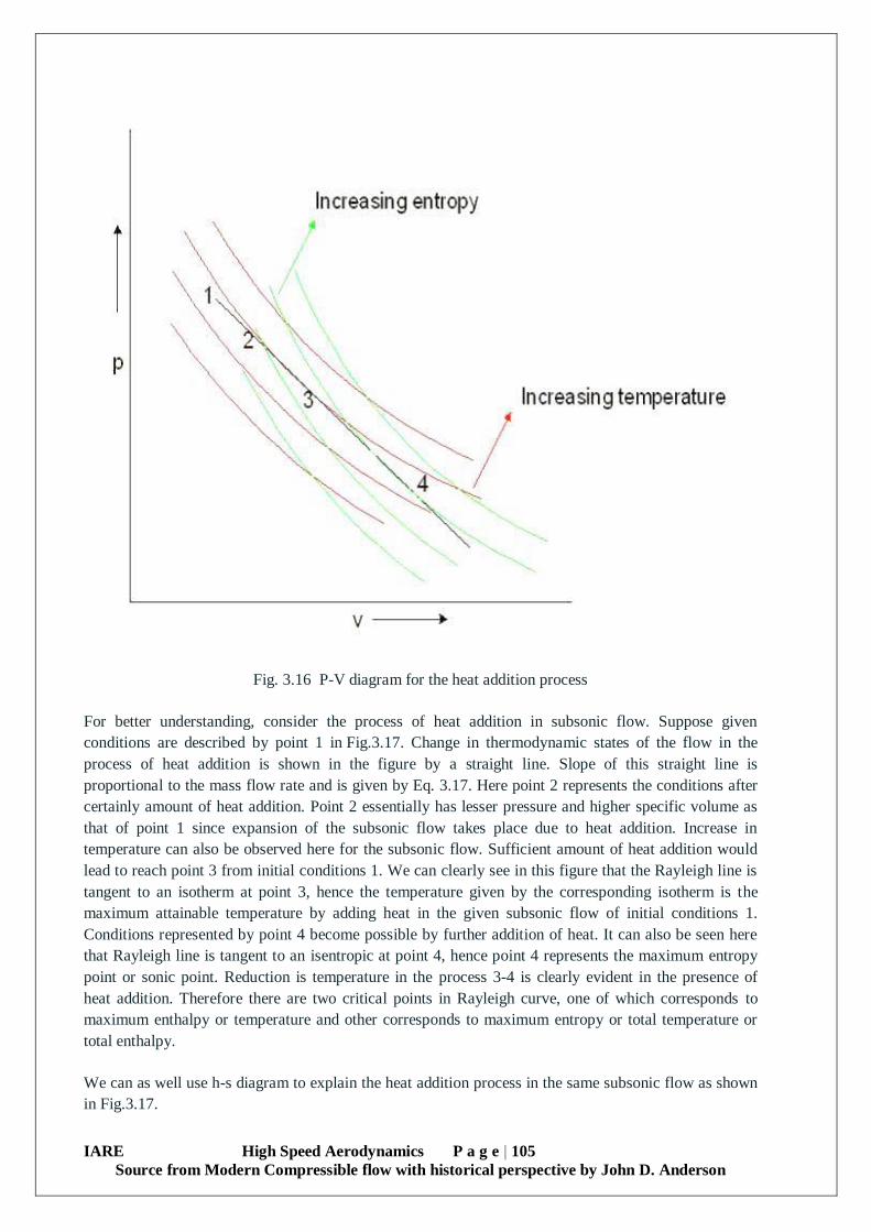
IARE High Speed Aerodynamics P a g e | 105
Source from Modern Compressible flow with historical perspective by John D. Anderson
Fig. 3.16 P-V diagram for the heat addition process
For better understanding, consider the process of heat addition in subsonic flow. Suppose given
conditions are described by point 1 in Fig.3.17. Change in thermodynamic states of the flow in the
process of heat addition is shown in the figure by a straight line. Slope of this straight line is
proportional to the mass flow rate and is given by Eq. 3.17. Here point 2 represents the conditions after
certainly amount of heat addition. Point 2 essentially has lesser pressure and higher specific volume as
that of point 1 since expansion of the subsonic flow takes place due to heat addition. Increase in
temperature can also be observed here for the subsonic flow. Sufficient amount of heat addition would
lead to reach point 3 from initial conditions 1. We can clearly see in this figure that the Rayleigh line is
tangent to an isotherm at point 3, hence the temperature given by the corresponding isotherm is the
maximum attainable temperature by adding heat in the given subsonic flow of initial conditions 1.
Conditions represented by point 4 become possible by further addition of heat. It can also be seen here
that Rayleigh line is tangent to an isentropic at point 4, hence point 4 represents the maximum entropy
point or sonic point. Reduction is temperature in the process 3-4 is clearly evident in the presence of
heat addition. Therefore there are two critical points in Rayleigh curve, one of which corresponds to
maximum enthalpy or temperature and other corresponds to maximum entropy or total temperature or
total enthalpy.
We can as well use h-s diagram to explain the heat addition process in the same subsonic flow as shown
in Fig.3.17.

IARE High Speed Aerodynamics P a g e | 106
Source from Modern Compressible flow with historical perspective by John D. Anderson
Fig.3.17 Rankine curve in h-s chart
3.7.1 Analysis of Critical Points of Rayleigh Curve
The same conservation equations for 1D heat addition can be re-written in differential form as,
For mass conservation equation
ρu = const = k
d(ρu) = 0 Mass Conservation
or
For momentum conservation equation
P + ρu2 = const
Momentum Conservation
IARE High Speed Aerodynamics P a g e | 107
Source from Modern Compressible flow with historical perspective by John D. Anderson
For energy conservation equation
dh + udu = dq Energy Conservation
P + vk2 = const
From laws of thermodynamics,
Tds = dh – vdp
However for point 3 (where Rankine line is tangent to an isotherm) dh=0 or dT=0, hence.
Tds = - vdp
From energy equation, for the same point we have,
Tds = udu
Hence,
- vdp = udu
Using differential form of mass conservation equation, we can replace du and we get,
However, we know that point 3 also lies on an the isotherm, we can calculate the slope of the isotherm
to obtain another expression for dP/dρ as
Hence we can put this dp/dρ in equation,
IARE High Speed Aerodynamics P a g e | 108
Source from Modern Compressible flow with historical perspective by John D. Anderson
This procedure provides a formal proof for the Mach number at the point which corresponds to
maximum temperature on Rayleigh curve. This expression also proves the fact that upper branch of
Rankine curve in h-s diagram corresponds to subsonic flow.
Similarly we can also prove that the sonic point (M=1), represented by point 4, corresponds to
maximumentropy.
We know the momentum conservation equation as
p + vk2 = const
The differential form of the same can be written as
dp + k2dv = const
Hence slope of Rankine line on p-v diagram is
We know that, at the point of maximum entropy, Rankine line is tangent to the isentropic. Hence slope
of theisentropic at point 4 is
pvγ = const
Differentiating this equation we get
vγdp + pγvγ-1dv = 0
Equating the slopes we get,
This expression proves the fact that maximum entropy point on Rayleigh curve corresponds to Mach
number 1 or sonic condition. We can extend our analysis about heat addition in subsonic flow and
attainment of maximum entropy as follows.
We know that addition of heat increases the total temperature and hence total enthalpy of the flow.
We know that,

IARE High Speed Aerodynamics P a g e | 109
Source from Modern Compressible flow with historical perspective by John D. Anderson
Hence the differential form of this equation is,
dh0 = dh + udu
However added heat gives rise to this change in total enthalpy, hence
dq = dh0
But dq = Tds.
Therefore
Tds = dh0 = dh + udu
However at the maximum entropy point, ds = 0, therefore dh0 = 0. Hence we can conclude that,
maximum entropy point also corresponds to maximum total enthalpy and hence total temperature point.
Therefore further addition of heat is not possible for the given mass flow rate. Hence point 4 also
represents the chocking condition. Change in upstream conditions takes place if we add heat more that
the heat requiredchocking the flow.
3.7.2 Choking of the flow with Heat Addition
It had been observed that the point of maximum entropy or maximum total temperature represents sonic
condition. This condition also represents the maximum possible heat addition in a flow. However
further increase in amount of heat addition in the flow decreases the mass flow rate through change in
upstream or inlet conditions. Expected streamline pattern for un-choked and choked flow is shown
in Figure.
Fig.3.18 Streamline pattern for unchocked condition.
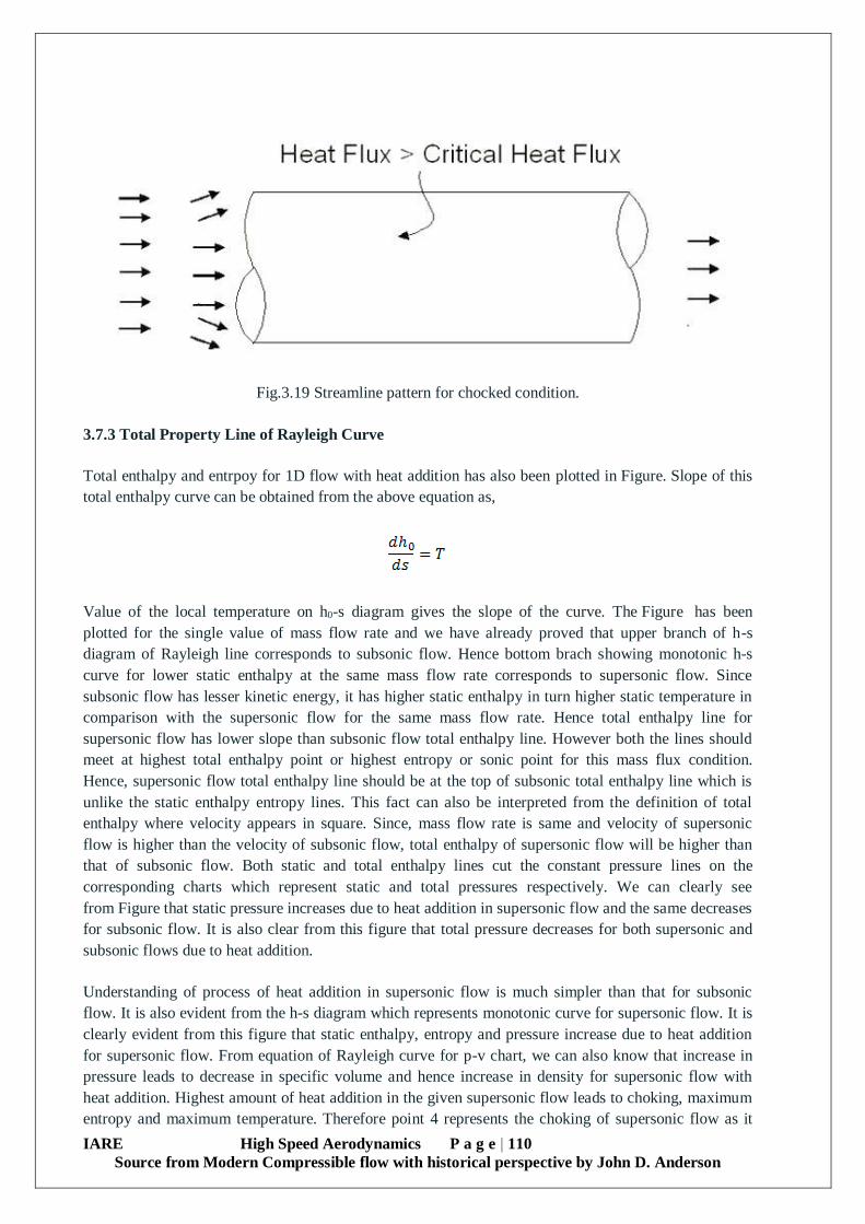
IARE High Speed Aerodynamics P a g e | 110
Source from Modern Compressible flow with historical perspective by John D. Anderson
Fig.3.19 Streamline pattern for chocked condition.
3.7.3 Total Property Line of Rayleigh Curve
Total enthalpy and entrpoy for 1D flow with heat addition has also been plotted in Figure. Slope of this
total enthalpy curve can be obtained from the above equation as,
Value of the local temperature on h0-s diagram gives the slope of the curve. The Figure has been
plotted for the single value of mass flow rate and we have already proved that upper branch of h-s
diagram of Rayleigh line corresponds to subsonic flow. Hence bottom brach showing monotonic h-s
curve for lower static enthalpy at the same mass flow rate corresponds to supersonic flow. Since
subsonic flow has lesser kinetic energy, it has higher static enthalpy in turn higher static temperature in
comparison with the supersonic flow for the same mass flow rate. Hence total enthalpy line for
supersonic flow has lower slope than subsonic flow total enthalpy line. However both the lines should
meet at highest total enthalpy point or highest entropy or sonic point for this mass flux condition.
Hence, supersonic flow total enthalpy line should be at the top of subsonic total enthalpy line which is
unlike the static enthalpy entropy lines. This fact can also be interpreted from the definition of total
enthalpy where velocity appears in square. Since, mass flow rate is same and velocity of supersonic
flow is higher than the velocity of subsonic flow, total enthalpy of supersonic flow will be higher than
that of subsonic flow. Both static and total enthalpy lines cut the constant pressure lines on the
corresponding charts which represent static and total pressures respectively. We can clearly see
from Figure that static pressure increases due to heat addition in supersonic flow and the same decreases
for subsonic flow. It is also clear from this figure that total pressure decreases for both supersonic and
subsonic flows due to heat addition.
Understanding of process of heat addition in supersonic flow is much simpler than that for subsonic
flow. It is also evident from the h-s diagram which represents monotonic curve for supersonic flow. It is
clearly evident from this figure that static enthalpy, entropy and pressure increase due to heat addition
for supersonic flow. From equation of Rayleigh curve for p-v chart, we can also know that increase in
pressure leads to decrease in specific volume and hence increase in density for supersonic flow with
heat addition. Highest amount of heat addition in the given supersonic flow leads to choking, maximum
entropy and maximum temperature. Therefore point 4 represents the choking of supersonic flow as it

IARE High Speed Aerodynamics P a g e | 111
Source from Modern Compressible flow with historical perspective by John D. Anderson
represented for the subsonic flow of same mass flow rate. It can be clearly concluded that the process of
heat addition can lead to supersonic flow to sonic state and further heat rejection to lower subsonic state.
Moreover, heat addition in subsonic flow can fetch the sonic conditions and further heat rejection leads
to supersonic condition. Hence possibility of reversible heat interaction eventually leads to trace the
complete h-s plot of Rayleigh curve for a given mass flow rate.
3.7.3 Effect of Change in Mass Flow Rate on T-S diagram for Rayleigh flow
Fig 3.20 A proposed experimental set up for 1D heat addition studies
The h-s plot shown for heat addition process in Figure belongs to a particular value of mass flow rate. If
we change the mass flow rate then the curve changes. Hence we need to find out the new curve in case
of decreased or increased mass flow rate conditions. Consider the proposed experimental set up shown
in Figure for the Rayleigh flow studies. Here we can change the mass flow rate by changing the
reservoir conditions (pressure and temperature) and also the exit pressure. During the experiment, gas
stored in the reservoir expands through the nozzle and achieves certain mass flow rate while flowing
through the constant area duct where heat addition takes place. We are going to learn the topic "flow
through nozzle" in detail in the coming lectures, however for now, we can assume that, mass flow rate
for subsonic flow can be increased by decreasing the exit pressure or increasing the reservoir pressure.
Similarly, we can increase the mass flow rate of supersonic flow by increase in reservoir pressure or by
decreasing the reservoir temperature.
Consider the case of subsonic flow with increased mass flow rate. Initial isentropic expansion in the
nozzle is given by the vertical line joining reservoir conditions and point 1 in Fig.3.21. If we add heat in
the flow through constant area duct then the process of heat addition is represented by the dotted curve
in the same figure. Suppose we increase the mass flow rate by decreasing exit pressure, then static
enthalpy or static temperature at the entry to the heating duct decreases. Hence length of the initial
vertical line increases and the nozzle exit conditions for subsonic flow are represented by 1'.
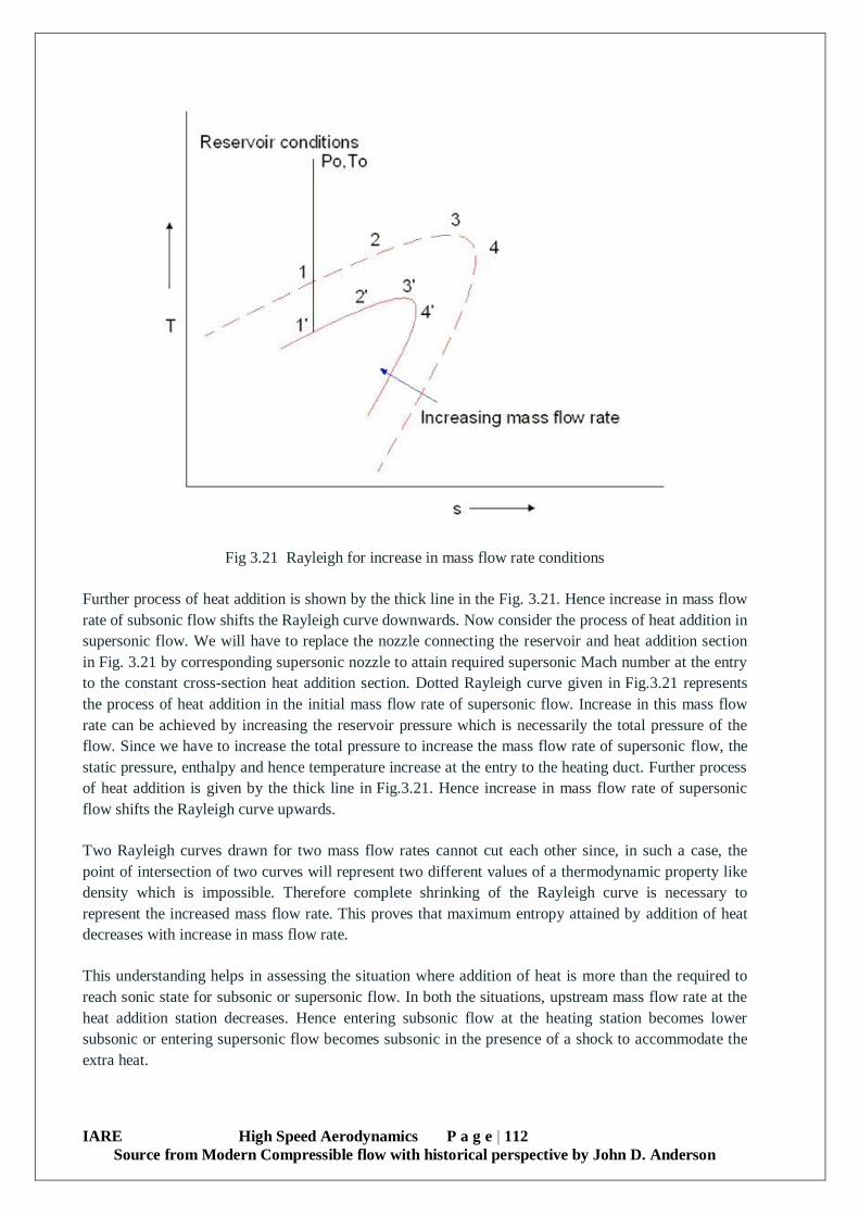
IARE High Speed Aerodynamics P a g e | 112
Source from Modern Compressible flow with historical perspective by John D. Anderson
Fig 3.21 Rayleigh for increase in mass flow rate conditions
Further process of heat addition is shown by the thick line in the Fig. 3.21. Hence increase in mass flow
rate of subsonic flow shifts the Rayleigh curve downwards. Now consider the process of heat addition in
supersonic flow. We will have to replace the nozzle connecting the reservoir and heat addition section
in Fig. 3.21 by corresponding supersonic nozzle to attain required supersonic Mach number at the entry
to the constant cross-section heat addition section. Dotted Rayleigh curve given in Fig.3.21 represents
the process of heat addition in the initial mass flow rate of supersonic flow. Increase in this mass flow
rate can be achieved by increasing the reservoir pressure which is necessarily the total pressure of the
flow. Since we have to increase the total pressure to increase the mass flow rate of supersonic flow, the
static pressure, enthalpy and hence temperature increase at the entry to the heating duct. Further process
of heat addition is given by the thick line in Fig.3.21. Hence increase in mass flow rate of supersonic
flow shifts the Rayleigh curve upwards.
Two Rayleigh curves drawn for two mass flow rates cannot cut each other since, in such a case, the
point of intersection of two curves will represent two different values of a thermodynamic property like
density which is impossible. Therefore complete shrinking of the Rayleigh curve is necessary to
represent the increased mass flow rate. This proves that maximum entropy attained by addition of heat
decreases with increase in mass flow rate.
This understanding helps in assessing the situation where addition of heat is more than the required to
reach sonic state for subsonic or supersonic flow. In both the situations, upstream mass flow rate at the
heat addition station decreases. Hence entering subsonic flow at the heating station becomes lower
subsonic or entering supersonic flow becomes subsonic in the presence of a shock to accommodate the
extra heat.
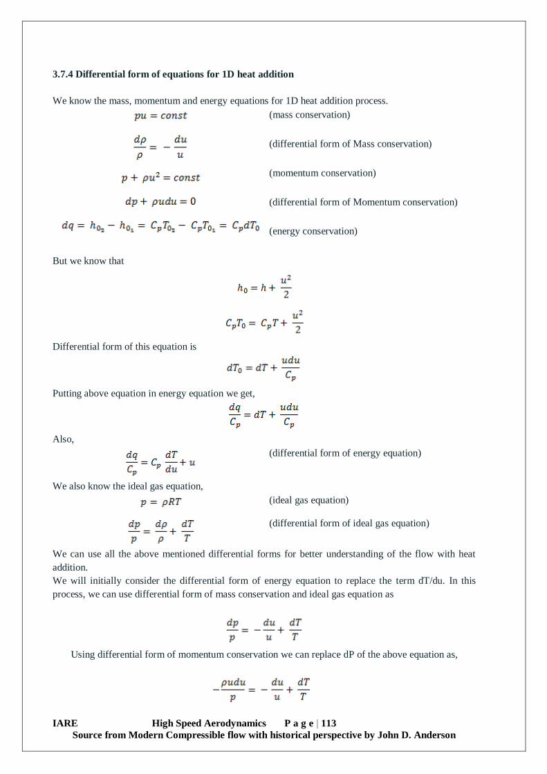
IARE High Speed Aerodynamics P a g e | 113
Source from Modern Compressible flow with historical perspective by John D. Anderson
3.7.4 Differential form of equations for 1D heat addition
We know the mass, momentum and energy equations for 1D heat addition process.
(mass conservation)
(differential form of Mass conservation)
(momentum conservation)
(differential form of Momentum conservation)
(energy conservation)
But we know that
Differential form of this equation is
Putting above equation in energy equation we get,
Also,
(differential form of energy equation)
We also know the ideal gas equation,
(ideal gas equation)
(differential form of ideal gas equation)
We can use all the above mentioned differential forms for better understanding of the flow with heat
addition.
We will initially consider the differential form of energy equation to replace the term dT/du. In this
process, we can use differential form of mass conservation and ideal gas equation as
Using differential form of momentum conservation we can replace dP of the above equation as,

IARE High Speed Aerodynamics P a g e | 114
Source from Modern Compressible flow with historical perspective by John D. Anderson
Hence,
Now we can use above equation to replace dT/du from differential form of energy equation. Hence
differential form of energy equation becomes,
But we know that,
Therefore,
Therefore, there are three cases viz. dq/du to be zero, positive or negative. Consider first case to start
with,
M = 1
This particular case can be interpreted as further change in velocity is impossible with heat addition.
Hence, dq/duto be zero represents maximum entropy or choking or sonic condition.
Now consider dq/du to be positive,
This particular case belongs to subsonic flow. Therefore for subsonic flow, dq/duis positive which
implicitly means velocity of the subsonic flow increases (du > 0) if heat is added in it (dq > 0). At the
same time, velocity of the subsonic flow decreases (du < 0) if heat is rejected from it (dq < 0).
Now consider dq/duto be negative,
IARE High Speed Aerodynamics P a g e | 115
Source from Modern Compressible flow with historical perspective by John D. Anderson
This particular case belongs to supersonic flow. Therefore for supersonic flow, dq/duis negative which
implicitly means velocity of the supersonic flow decreases (du < 0) if heat is added in it (dq > 0). At the
same time, velocity of the supersonic flow increases (du > 0) if heat is rejected from it (dq < 0).
Now consider Equation
we can clearly see the existence of three cases here also, in which dT/du can be either zero, positive, or
negative. Consider dT/duto be zero so,
Hence for this condition we will have dT/du zero means dT = 0. This condition corresponds to
maximum temperature attained by heat addition. From𝑀 = 𝛾−1/2, it becomes clear that, this condition
belongs to subsonic flow where further increase in temperature is not possible with heat addition.
Now consider the case where, dT/du is positive. Hence
𝑇
𝑢>
𝑢
𝑅
𝑀2 < 𝛾−1/2This means that for subsonic flow till𝑀2 < 𝛾−1/2, dT/du is positive. We have already seen
that for subsonic flow du is positive. This proves that, for subsonic flow, dT is positive till𝑀2 < 𝛾−1/2.
Now for the third case with dT/du is negative, we will get > 𝛾−1/2 . However for subsonic flow du is
always positive, hence for any subsonic Mach number which is 𝑀 > 𝛾−1/2 till M = 1, dT is negative.
Therefore in this range of subsonic Mach number added heat decreases temperature and increases the
velocity. However from present expression, dT/du is negative for all> 𝛾−1/2 . Hence for supersonic
flows also dT/du is negative. But we have already seen that du is negative for supersonic flow with heat
addition, hence dT is positive for supersonic flow. Hence externally added heat in supersonic flow
decreases velocity and increases temperature.
We can modify the right hand side of Equation as
Hence, Equation can be written as,
The proof about all the critical points can be achieved from this expression as well.
IARE High Speed Aerodynamics P a g e | 116
Source from Modern Compressible flow with historical perspective by John D. Anderson
UNIT – IV
APPLICATIONS OF COMPRESSIBLE FLOWS AND NUMERICAL TECHNIQUES
4.1 Small perturbation equations for subsonic, transonic, supersonic and hypersonic flow
4.1.1 Small-Perturbation Theory
A great number of problems of interest in compressible fluid mechanics are concerned with the
perturbation of a known flow pattern. The most common case is that of uniform, steady flow.
Let U denote the uniform flow velocity, which is directed parallel to the x -axis. The density, pressure,
and temperature are also assumed to be uniform, and are denoted ρ∞, P∞ and T∞ respectively. The
corresponding sound speed is c∞ , and the Mach number is Ma∞ =U/c∞
Finally,the velocity field of the unperturbed flow pattern is
u = U,
v =0
Suppose that a solid body, such as an airfoil, is placed in the aforementioned flow pattern. The cross-
section of the body is assumed to be independent of the Cartesian coordinate Z. The body disturbs the
flow pattern, and changes its velocity field, which is now written
u = U+uꞌ,
v = vꞌ
where uꞌ and vꞌ are known as induced velocity components. We are interested in situations in
which
uꞌ/U <<1 and vꞌ/V<<1
Equation can be combined with the previous two equations to give
𝐶2 = 𝐶∞2 −
1
2(𝛾 − 1)(2𝑈𝑢′ + 𝑢′2
+ 𝑣′2)
It then follows from Equation that
(1 − 𝑀𝑎∞2 )
𝜕𝑢′
𝜕𝑥+
𝜕𝑣′
𝜕𝑦
= 𝑀𝑎∞2 [(𝛾 − 1)
𝑢′
𝑈+ (
𝛾 + 1
2) (
𝑢′
𝑈)
2
+ (𝛾 − 1
2) (
𝑣′
𝑈)
2
]𝜕𝑢′
𝜕𝑥
+ 𝑀𝑎∞2 [(𝛾 − 1)
𝑣′
𝑈+ (
𝛾 + 1
2) (
𝑣′
𝑈)
2
+ (𝛾 − 1
2) (
𝑢′
𝑈)
2
]𝜕𝑢′
𝜕𝑦
+ 𝑀𝑎∞2
𝑢′
𝑈(1 −
𝑢′
𝑈) (
𝜕𝑢′
𝜕𝑦+
𝜕𝑣′
𝜕𝑥)
The previous equation is exact. However, if uꞌ/U and vꞌ/V are small then it becomes possible to neglect
many of the terms on the right-hand side. For instance, neglecting terms that are third-order in small
quantities, we obtain
IARE High Speed Aerodynamics P a g e | 117
Source from Modern Compressible flow with historical perspective by John D. Anderson
(1 − 𝑀𝑎∞2 )
𝜕𝑢′
𝜕𝑥+
𝜕𝑣′
𝜕𝑦≃ 𝑀𝑎∞
2 (𝛾 + 1)𝑢′
𝑈
𝜕𝑢′
𝜕𝑥+ 𝑀𝑎∞
2 (𝛾 − 1)𝑢′
𝑈
𝜕𝑣′
𝜕𝑦+ 𝑀𝑎∞
2𝑣′
𝑈(
𝜕𝑢′
𝜕𝑦+
𝜕𝑣′
𝜕𝑥)
Furthermore, if we neglect terms that are second-order in small quantities then we get the linear
equation
1 − 𝑀𝑎∞2 (
𝜕𝑢′
𝜕𝑥+
𝜕𝑣′
𝜕𝑦) ≃ 0
Note, however, than in so-called transonic flow, where𝑀𝑎∞ ≃ 1 , the coefficient of𝜕𝑢′
𝜕𝑥⁄ on the left-
hand side of Equation becomes very small. In this situation, it is not possible to neglect the first term on
the right-hand side. However, the condition𝑀𝑎∞ ≃ 1 does not affect the term 𝜕𝑣′
𝜕𝑦⁄ on the left-hand
side of Equation, and so the other terms on the right-hand side can still be neglected. Thus, transonic
flow is governed by the non-linear equation
On the other hand, subsonic (i.e.,Ma∞<1 ) and supersonic flow (i.e., Ma∞>1 ) are both governed by
Equation . Another situation in which certain terms on the right-hand side of Equation must be retained
is hypersonic flow (i.e., Ma∞>>1 ). This follows because, although uꞌ/U and vꞌ/V are small, their
products with𝑀𝑎∞2 can still be non-negligible. Roughly speaking, Equation is valid for 0 ≤ Ma∞ ≤ 0.8
and 1.2 ≤ Ma∞ ≤ 5 and . In other words, transonic flow corresponds to 0.8 ≤ Ma∞ ≤ 1.2 , and
hypersonic flow to Ma∞>5.
The pressure coefficient is defined
Equation implies that
Where
.
Moreover, Equation yields
Where Ma = q/c . The previous two equations can be combined to give
Hence, we obtain

IARE High Speed Aerodynamics P a g e | 118
Source from Modern Compressible flow with historical perspective by John D. Anderson
which reduces to
Using the binomial expansion on the expression in square brackets, and neglecting terms that are third-
order, or higher, in small quantities, we obtain
For two-dimensional flows, in the limit in which Equation is valid, it is consistent to retain only first-
order terms in the previous equation, so that
Let
f(x,y) = 0
be the equation of the surface of the solid body that perturbs the flow. At the surface, the velocity vector
of the flow must be perpendicular to the local normal: that is, the flow must be tangential to the surface.
In other words,
𝑞. ∇𝑓 = 0 which reduces to
Neglecting uꞌ with respect to U , we obtain
Where dy/dx is the slope of the surface, and vꞌ/u the approximate slope of a streamline.
Now, the body has to be thin in order to satisfy our assumption that the induced velocities are relatively
small. This implies that the coordinate y differs little from zero (say) on the surface of the body. Hence,
we can write
in the immediate vicinity of the surface. Within the framework of small-perturbation theory, it is
consistent to neglect all terms on the right-hand side of the previous equation after the first. Hence, the
boundary condition reduces to

IARE High Speed Aerodynamics P a g e | 119
Source from Modern Compressible flow with historical perspective by John D. Anderson
respectively.
Because a homenergic, homentropic flow pattern is necessarily irrotational, we can write
Where ϕ is the perturbed velocity potential.
It follows that
U2= −𝜕∅
𝜕𝑥,
v2= −𝜕∅
𝜕𝑦,
Hence, Equationsbecome
4.2 Experimental characteristics of airfoils in compressible flow
4.2.1 Linearization of Velocity Potential Equation
Consider the steady irrotational flow around the thin aerofoil as shown in Fig. 4.1
Fig. 4.1 Schematic of the perturbed velocity field.
At location A, velocity is only in x direction. However, presence of body perturbs the components of
velocity at location B. Let’s represent the general velocity field as,
IARE High Speed Aerodynamics P a g e | 120
Source from Modern Compressible flow with historical perspective by John D. Anderson
here,Vx = V∞+uꞌ and uꞌ, vꞌ, wꞌ are the perturbed velocities in the x, y and z directions respectively such
that.
Vy = vꞌ
Vw = wꞌ Since the velocity field is irrotational, we can represent the velocity field using gradient of velocity
potential as,
Let the perturbed velocity field be presented by perturbed velocity potential, ϕ. Hence,
Therefore,
Φ(x, y, z) = V∞ x + ϕ(x, y, z)
Such that,
and
, ,
We can use these expressions in the known velocity potential equation.
This expression in the form of perturbed velocity potential can be written as,

IARE High Speed Aerodynamics P a g e | 121
Source from Modern Compressible flow with historical perspective by John D. Anderson
or,
But we know that, total enthalpy is constant in flow field. We can use this fact to represent the speed of
sound encountered in the above equation as,
ho = const.
Using this expression and further simplification, Eq. can be written as,
The equation is the exact equation for steady irrotational flow around the thin configurations.
We can simplify this equation, since the perturbed velocities, uꞌ, vꞌ and wꞌare small in comparison with
the freestream velocity V∞ .

IARE High Speed Aerodynamics P a g e | 122
Source from Modern Compressible flow with historical perspective by John D. Anderson
Hence,
, and <<1
So,
This approximations leads to two facts,
1. Except for the Transonic flows (Flows having Mach number in the range 0.8 to 1.2)
2. If Mach number of the flow is less than 5.0
,
For these two facts we get,
Or,
This is the linear equation and this approximation is valid for steady irrotational subsonic and
supersonic flows under the assumption of small perturbation.
4.3 Supercritical airfoil
A Supercritical airfoil is an airfoil designed, primarily, to delay the onset of wave drag inthe transonic
speed range. Supercritical airfoils are characterized by their flattened upper surface, highly cambered
(curved) aft section, and smaller leading edge radius compared with traditional airfoil shapes. The
supercritical airfoils were designed in the 1960s, by then NASA Engineer Richard Whitcomb, and were
first tested on a modified North American T-2C Buckeye. After this first test, the airfoils were tested at
higher speeds on the TF-8A Crusader While the design was initially developed as part of the supersonic
transport (SST) project at NASA, it has since been mainly applied to increase the fuel efficiency of
many high subsonic aircraft. The supercritical airfoil shape is incorporated into the design of a
supercritical wing.
Supercritical airfoils feature four main benefits: they have a higher drag divergence Machnumber,they
develop shock waves further aft than traditional airfoils,they greatly reduce shock-induced boundary
layer separation, and their geometry allows for more efficient wing design (e.g., a thicker wing and/or
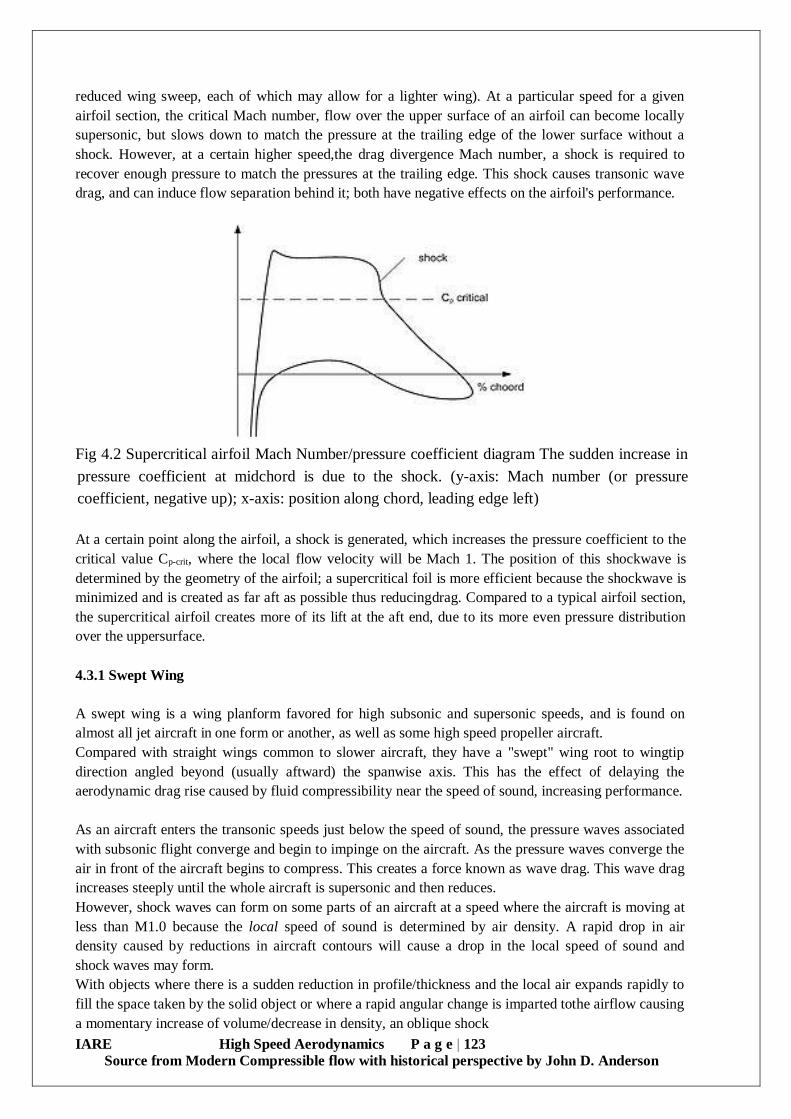
IARE High Speed Aerodynamics P a g e | 123
Source from Modern Compressible flow with historical perspective by John D. Anderson
reduced wing sweep, each of which may allow for a lighter wing). At a particular speed for a given
airfoil section, the critical Mach number, flow over the upper surface of an airfoil can become locally
supersonic, but slows down to match the pressure at the trailing edge of the lower surface without a
shock. However, at a certain higher speed,the drag divergence Mach number, a shock is required to
recover enough pressure to match the pressures at the trailing edge. This shock causes transonic wave
drag, and can induce flow separation behind it; both have negative effects on the airfoil's performance.
Fig 4.2 Supercritical airfoil Mach Number/pressure coefficient diagram The sudden increase in
pressure coefficient at midchord is due to the shock. (y-axis: Mach number (or pressure
coefficient, negative up); x-axis: position along chord, leading edge left)
At a certain point along the airfoil, a shock is generated, which increases the pressure coefficient to the
critical value Cp-crit, where the local flow velocity will be Mach 1. The position of this shockwave is
determined by the geometry of the airfoil; a supercritical foil is more efficient because the shockwave is
minimized and is created as far aft as possible thus reducingdrag. Compared to a typical airfoil section,
the supercritical airfoil creates more of its lift at the aft end, due to its more even pressure distribution
over the uppersurface.
4.3.1 Swept Wing
A swept wing is a wing planform favored for high subsonic and supersonic speeds, and is found on
almost all jet aircraft in one form or another, as well as some high speed propeller aircraft.
Compared with straight wings common to slower aircraft, they have a "swept" wing root to wingtip
direction angled beyond (usually aftward) the spanwise axis. This has the effect of delaying the
aerodynamic drag rise caused by fluid compressibility near the speed of sound, increasing performance.
As an aircraft enters the transonic speeds just below the speed of sound, the pressure waves associated
with subsonic flight converge and begin to impinge on the aircraft. As the pressure waves converge the
air in front of the aircraft begins to compress. This creates a force known as wave drag. This wave drag
increases steeply until the whole aircraft is supersonic and then reduces.
However, shock waves can form on some parts of an aircraft at a speed where the aircraft is moving at
less than M1.0 because the local speed of sound is determined by air density. A rapid drop in air
density caused by reductions in aircraft contours will cause a drop in the local speed of sound and
shock waves may form.
With objects where there is a sudden reduction in profile/thickness and the local air expands rapidly to
fill the space taken by the solid object or where a rapid angular change is imparted tothe airflow causing
a momentary increase of volume/decrease in density, an oblique shock

IARE High Speed Aerodynamics P a g e | 124
Source from Modern Compressible flow with historical perspective by John D. Anderson
wave is generated. This is why shock waves are often associated with the part of a fighter aircraft
cockpit canopy with the highest local curvature, appearing immediately behind this point.
At the point where the density drops, the local speed of sound correspondingly drops and a shock wave
can form. This is why in conventional wings, shock waves form first after the maximum
Thickness/Chord and why all airliners designed for cruising in the transonic range (above M0.8) have
supercritical wings that are flatter on top resulting in minimized angular change of flow to upper surface
air. The angular change to the air that is normally part of lift generation is decreased and this lift
reduction is compensated for by deeper curved lower surfaces accompanied by a reflex curve at the
trailing edge. This results in a much weaker standing shock wave towards the rear of the upper wing
surface and a corresponding increasein critical Mach number.
4.3.2 Second order equation for transonic flows
The numerical solution of the compressible Euler and Navier-Stokes equations in primitive variables
form requires the use of artificial viscosity or upwinding. Methods that are first-order- accurate are too
dissipative and reduce the effective Reynolds number substantially unless a very fine grid is used. A
first-order finite element method for the solution of the Euler and Navier- Stokes equations can be
constructed by adding Laplacians of the primitive variables to the governing equations. Second-order
schemes may require fourth-order dissipation and higher- order elements. A finite element approach is
proposed in which the fourth-order dissipation is recast as the difference of two Laplacian operators,
allowing the use of bilinear elements. The Laplacians of the primitive variables of the first-order
scheme are thus balanced by additional terms obtained from the governing equations themselves, tensor
identities or other forms of nodal averaging.
4.3 Area Rule
Whitcomb’s Area Rule
The Whitcomb area rule, also called the transonic area rule, is a design technique used to reducean
aircraft's drag transonic and supersonic speeds, particularly between Mach 0.75 and 1.2.This is one of
the most important operating speed ranges for commercial and military fixed-wingaircraft today, with
transonic acceleration being considered an important performance metric for combat aircraft and
necessarily dependent upon transonic drag.
At high-subsonic flight speeds, the local speed of the airflow can reach the speed of sound where the
flow accelerates around the aircraft body and wings. The speed at which this development occurs varies
from aircraft to aircraft and is known as the critical Mach number. Theresulting shock waves formed at
these points of sonic flow can greatly reduce power, which is experienced by the aircraft as a sudden
and very powerful drag, called wave drag. To reduce the number and power of these shock waves, an
aerodynamic shape should change in crosssectional area as smoothly as possible.
The area rule says that two airplanes with the same longitudinal cross-sectional area distribution have
the same wave drag, independent of how the area is distributed laterally (i.e. in the fuselage or in the
wing). Furthermore, to avoid the formation of strong shock waves, this total area distribution must be
smooth. As a result, aircraft have to be carefully arranged so that at the location of the wing, the
fuselage is narrowed or "waisted", so that the total area doesn't change much. Similar but less
pronounced fuselage waisting is used at the location of a bubble canopy and perhaps the tail surfaces.
IARE High Speed Aerodynamics P a g e | 125
Source from Modern Compressible flow with historical perspective by John D. Anderson
The area rule also holds true at speeds exceeding the speed of sound, but in this case the body
arrangement is in respect to the Mach line for the design speed. For example, consider that at Mach 1.3
the angle of the Mach cone formed off the body of the aircraft will be at about μ = arcsin(1/M) = 50.3°
(μ is the angle of the Mach cone, or simply Mach angle). In this case the "perfect shape" is biased
rearward; therefore, aircraft designed for high speed cruise usually have wings towards the rear.A
classic example of such a design is the Concorde. When applying the transonic area rule, the condition
that the plane defining the cross-section meets the longitudinal axis at the Mach angle μ no longer
prescribes a unique plane for μ other than the 90° given by M= 1. The correct procedure is to average
over all possible orientations of the intersecting plane.
4.4 Theory of characteristics (method of characteristics), determination of the
characteristic lines and compatibility equations,
Theory of characteristics
4.4.1 Introduction
The method of characteristics has been used for many years to compute supersonic irrotational flows.
Although the method has a strong analytical basis, its practical implementation is, essentially, always
numerical and it is then used to compute the values of the flow variables at a series of distinct points in
the flow rather than continuously throughout the flow field.
Let’s consider a general steady two-dimensional irrotational flowfield. We have already derived
thevelocity potential (φ) equation for such flowfield.
Consider the change in any flow variable, f, df which can be determined by small changes in the
coordinates dx and dy as illustrated in Figure. The change in the variable, df,
If 𝑓 = 𝜕∅𝜕𝑥⁄ then this will give:
But 𝑢 = 𝜕∅𝜕𝑥⁄ so this equation gives:
Similarly if 𝑓 = 𝜕∅𝜕𝑦⁄ then this will give:

IARE High Speed Aerodynamics P a g e | 126
Source from Modern Compressible flow with historical perspective by John D. Anderson
But 𝑣 = 𝜕∅𝜕𝑦⁄ so this equation gives:
Now consider eqs. which involve second derivatives of φ and can be solved using Cramer’s Rule. For
example
In general, this equation can be solved for any chosen values of dx and dy , i.e., for any chosen
direction, to give 𝜕2∅ 𝜕𝑥𝜕𝑦⁄ at a selected point in the flow. However, it is possible to
have𝜕2∅ 𝜕𝑥𝜕𝑦⁄ indeterminate in certain directions. More over this differential is expected to be finite at
that point. Hence in these directions, eq. must give an indeterminate value.
Let’s consider the denominator of equation since along a particular direction𝜕2∅ 𝜕𝑥𝜕𝑦⁄ is
indeterminate. Hence the denominator should be zero, as:
Dividing by(dx)2 gives:
The subscript 'ch' on dy/dx indicates that the slope of the characteristic line or a specific direction is
being considered along which differentials are indeterminate. Solving above equation we get:
Let’srepresent the component of velocities in terms of velocity vector and angle made by the streamline
with co-ordinate axes as,
V2= u2+v2
u = V cosθ
v = V sinθ
Hence, we get the same equation for slope as,
where, M=V/a.
We can introduce the local Mach angle, a, where (M=1/sinα, √𝑀2 − 1 =1/tan α) by replacing Mach
number as,
IARE High Speed Aerodynamics P a g e | 127
Source from Modern Compressible flow with historical perspective by John D. Anderson
After much manipulation and rearrangement, it can be shown that this equation gives:
(𝑑𝑦
𝑑𝑥)
𝑐ℎ= tan (𝜃±∝)
There are two characteristic lines. This clearly means that the characteristic lines or lines along which
derivatives are inderminate makes Mach angle with the streamline. Hence the net angle made by the
characteristic line with the x-axis is the summation of the angle made by the streamline with x-axis and
angle made by the Mach wave with streamline. Hence Mach waves are the characteristic lines.
4.4.2 Governing Equation
We know about the direction of the characteristic line obtained from the indeterminacy of the equation
for zero denominators. However finiteness of the differential compels the zero value of the numerator.
This condition evolves the equation to be solved along the characteristic lines.
Hence for the numerator equation we have,
Substituting for slope (dy/dx) of the characteristic lines from equation that gives:
Substituting this expression in equation we get,

IARE High Speed Aerodynamics P a g e | 128
Source from Modern Compressible flow with historical perspective by John D. Anderson
This is the equation governing the changes in the variables along the characteristic lines. It can be noted
that it is an ordinary differential equation whereas the original equation, velocity potential equation, was
a partial differential equation.
We have already seen the solution for equation during consideration of expansion fan. On the similar
line, the integration of equation leads to,
This is the simple algebraic equation which we will have to solve along the characteristic line.
Following figure represents the details of the characteristic lines.
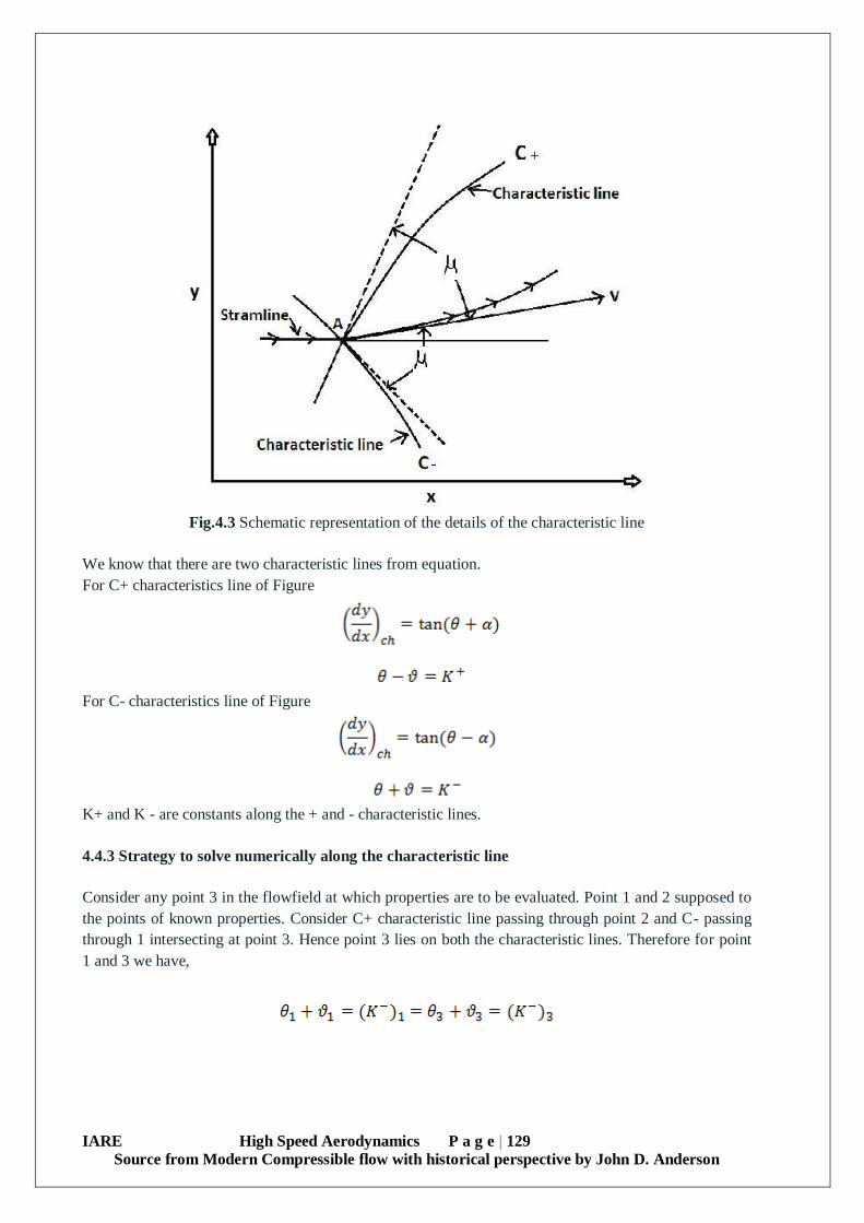
IARE High Speed Aerodynamics P a g e | 129
Source from Modern Compressible flow with historical perspective by John D. Anderson
Fig.4.3 Schematic representation of the details of the characteristic line
We know that there are two characteristic lines from equation.
For C+ characteristics line of Figure
For C- characteristics line of Figure
K+ and K - are constants along the + and - characteristic lines.
4.4.3 Strategy to solve numerically along the characteristic line
Consider any point 3 in the flowfield at which properties are to be evaluated. Point 1 and 2 supposed to
the points of known properties. Consider C+ characteristic line passing through point 2 and C- passing
through 1 intersecting at point 3. Hence point 3 lies on both the characteristic lines. Therefore for point
1 and 3 we have,
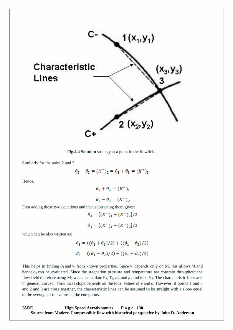
IARE High Speed Aerodynamics P a g e | 130
Source from Modern Compressible flow with historical perspective by John D. Anderson
Fig.4.4 Solution strategy at a point in the flowfield.
Similarly for the point 2 and 3
Hence,
First adding these two equations and then subtracting them gives:
which can be also written as:
This helps in finding θ3 and v3 from known properties. Since v3 depends only on M, this allows M3and
hence a3 can be evaluated. Since the stagnation pressure and temperature are constant throughout the
flow field therefore using M3 we can calculate P3, T3, a3, and ρ3 and then V3. The characteristic lines are,
in general, curved. Their local slope depends on the local values of v and θ. However, if points 1 and 3
and 2 and 3 are close together, the characteristic lines can be assumed to be straight with a slope equal
to the average of the values at the end points.

IARE High Speed Aerodynamics P a g e | 131
Source from Modern Compressible flow with historical perspective by John D. Anderson
Since θ3 and a3 are determined by solving above two equations we can determine x3 and y3.
The procedure discussed above was for an "internal" point, i.e., a point 3 in the flow field that did not lie
on a boundary. If a point lies on the boundary, the flow direction at this point will be determined by the
slope of the boundary, e.g., consider the point 5 shown in Fig. 33.3 which lies on a solid wall. The flow
direction at this point θ5 is equal to the slope of the wall as indicated. Consider the characteristic line
between points 4 and 5 as shown in the same figure. Since (K - )4 = (K - )5 it follows that:
Fig. 4.5 Demonstration of wall boundary condition
However, θ5 is known, hence v5 is given by:
With v5 determined, the values of all the flow properties at 5 can be determined as discussed before. The
characteristic line between 4 and 5 is, of course, assumed to be straight which determines the position of
the point 5.
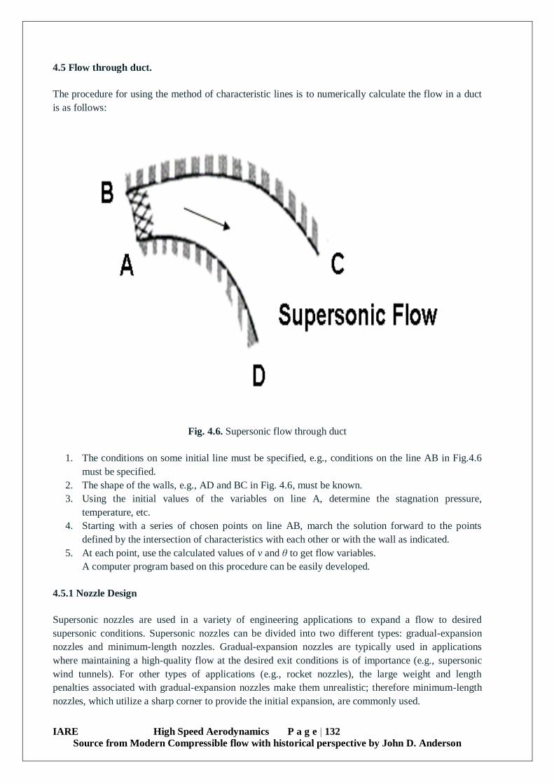
IARE High Speed Aerodynamics P a g e | 132
Source from Modern Compressible flow with historical perspective by John D. Anderson
4.5 Flow through duct.
The procedure for using the method of characteristic lines is to numerically calculate the flow in a duct
is as follows:
Fig. 4.6. Supersonic flow through duct
1. The conditions on some initial line must be specified, e.g., conditions on the line AB in Fig.4.6
must be specified.
2. The shape of the walls, e.g., AD and BC in Fig. 4.6, must be known.
3. Using the initial values of the variables on line A, determine the stagnation pressure,
temperature, etc.
4. Starting with a series of chosen points on line AB, march the solution forward to the points
defined by the intersection of characteristics with each other or with the wall as indicated.
5. At each point, use the calculated values of v and θ to get flow variables.
A computer program based on this procedure can be easily developed.
4.5.1 Nozzle Design
Supersonic nozzles are used in a variety of engineering applications to expand a flow to desired
supersonic conditions. Supersonic nozzles can be divided into two different types: gradual-expansion
nozzles and minimum-length nozzles. Gradual-expansion nozzles are typically used in applications
where maintaining a high-quality flow at the desired exit conditions is of importance (e.g., supersonic
wind tunnels). For other types of applications (e.g., rocket nozzles), the large weight and length
penalties associated with gradual-expansion nozzles make them unrealistic; therefore minimum-length
nozzles, which utilize a sharp corner to provide the initial expansion, are commonly used.

IARE High Speed Aerodynamics P a g e | 133
Source from Modern Compressible flow with historical perspective by John D. Anderson
Fig. 4.7 Types of nozzles.
For both gradual-expansion and minimum-length nozzles, the flow can be divided into simple and non-
simple regions. A non-simple region is characterized by Mach wave reflections and intersections. In
order to meet the requirement of uniform conditions at the nozzle exit, it is desirable to minimize the
non-simple region as much as possible. This can be performed by designing the nozzle surface such that
Mach waves (e.g., characteristics) are not produced or reflected while the flow is straightened. The
Method of Characteristics is therefore applied to allow the design of a supersonic nozzle which meets
these requirements.
4.5.2 Design of Minimum-Length Nozzle (MLN)
It should be noted that for this two-dimensional nozzle configuration, flow symmetry implies that only
half of the nozzle is physically required, assuming that the characteristic reflections in the non-simple
region are maintained. Therefore, we can make the assumption of a half-symmetric minimum-length
nozzle, in which a nozzle flap is extended from the symmetry plane such that it meets the length
requirement for the last characteristic intersecting the nozzle surface.
Fig.4.8. Schematic of characteristic lines for MLN.

IARE High Speed Aerodynamics P a g e | 134
Source from Modern Compressible flow with historical perspective by John D. Anderson
4.5.3 Implementation of Method of Characteristics
The two-dimensional Method of Characteristics is a relatively simple analytical model for analyzing
supersonic two-dimensional flow. This analysis is performed by considereing the characteristic lines in
the flow. Points along each characteristic have five important properties: M (Mach number), θ (flow
angle), ν (Prandtl-Meyer function), and x and y (position). For the assumption of steady, supersonic, we
know that,
𝜃 ± 𝑣 = 𝑐𝑜𝑛𝑠𝑡𝑎𝑛𝑡
The constant for summation can be said to be K+ and for subtraction to be K-. These constants are the
Riemann invariants, which are constant along the characteristics C+ and C-.
4.5.4 Design of Gradual expansion nozzle
The steps involved in this calculation are precisely same as those used for the minimum length nozzle
except for the fact that the expansion fan at the sharp corner is now replaced by a series of right running
characteristic lines originating from the arc of the circle. One major assumption that has been made here
is that a characteristic originating from any point on the expansion section is always reflected from the
axis in such a way that it reaches the straightening portion of the nozzle. Multiple reflections of
characteristic lines within the smooth expansion portion of the nozzle would make the problem much
complicated without really improving the results much.
4.5.4 Governing equation in 2-D
For subsonic flows density has a known constant value, i.e. it is no longer an unknown.. Conservation of
Mass: For constant density which means that the velocity field of an incompressible flow should be
divergence free, this is known as the divergence free constraint in CFD literature.
We have .
Note that there is no time derivative in the continuity equation even for unsteady flows, which is one of
the reasons that make numerical solution of incompressible flows difficult.
Conservation of Linear Momentum:
Dividing the equation by density we get the following form of the Navier-Stokes equation.
The term on the right hand side is known as the convective term. It is the term which makes the Navier-
Stokes equation nonlinear. For diffusion dominated flows the convective term can be dropped and the
simplified equation is called the Stokes equation, which is linear. Stokes equations can be used to model
very low speed flows known as creeping flows or flows with very small length scales (micro or nano
flows) where Reynolds number is small. Convectiondominated flows, which are typically characterized
IARE High Speed Aerodynamics P a g e | 135
Source from Modern Compressible flow with historical perspective by John D. Anderson
by high Reynolds numbers, are much more difficult to solve numerically compared to diffusion
dominated flows. For most solid mechanics problems convection (flow of material) does not exist, which
is the main reason of the differences seen in mathematical modeling (Eulerian vs. Lagrangian
formulations) and in numerical solution techniques (e.g. need for up winding) used in the disciplines of
fluid and solid mechanics. Conservation of Energy: Conservation of energy can be simplified by
considering the fact that density is constant for incompressible. Note that for incompressible flows. Here
it is important to note that for incompressible flows equation of state does not exist. In practice this
means that the energy equation is decoupled from the other two equations. Therefore we can first solve
continuity and Navier-Stokes equations to find the unknown velocity and pressure distribution without
knowing the temperature (We assume that fluid properties are taken to be constant, i.e. not functions of
temperature. If fluid properties change with temperature all equations becomes coupled as in the case
ofcompressible flows). After finding the velocity field, energy equation can be solved by itself to find
the temperature distribution. However for buoyancy driven flows (natural convection) where the density
changes due to temperature variations are considered in the body force term of the momentum equation
(Boussinesq approximation), all three conservation equations again become coupled. Heat transfer and
therefore the energy equation is not always a primary concern in an incompressible flow. For isothermal
(constant temperature) incompressible flows energy equation (and therefore temperature) can be
dropped and only the mass and linear momentum equations are solved to obtain the velocity and
pressure fields. Numerical solution of incompressible flows is usually considered to be more difficult
compared to compressible flows. The main numerical difficulty of solving incompressible flows lies in
the role of pressure. For incompressible flows pressure is no longer a thermodynamic quantity and it
cannotbe related to density or temperature through an equation of state. It just establishes itself
instantaneously in a flow field so that the velocity field always remains divergence free. In the continuity
equation there is no pressure term and in the momentum equation there are only the derivatives of
pressure, but not the pressureitself.This means that the actual value of pressure in an incompressible
flow solution is not important only the changes of pressure in space are important. Additionally there is
no time derivative of pressure, even for incompressible flows.

IARE High Speed Aerodynamics P a g e | 136
Source from Modern Compressible flow with historical perspective by John D. Anderson
UNIT-V
EXPERIMENTAL METHODS IN COMPRESSIBLE FLOWS
With the advancement of aerospace vehicles, the human’s dream is to fly faster and higher. Speed of
manned and unmanned flight vehicles has increased by some orders of magnitude over the last few
decades. As the speed of the vehicle is increased, the aerodynamic environment becomes increasingly
hostile. At speeds around the local speed of sound (Transonic) and higher (Supersonic), the
aerodynamic loads increase and their distributions change. When the speed of the vehicle becomes
several times higher than the speed of sound (Hypersonic), additional problem of aerodynamic heating
demands the change in design geometry and materials. At still higher speeds,the behavior of air begins
to change significantly; both physically and chemically. There is a conventional ‘rule-of-thumb’ that
defines the flow regimes based on the free stream Mach number
i.e.Subsonic:0<M∞<0.8;Transonic:0.8<M∞>1.2 Supersonic:1.2>M∞>5;Hypersonic:M∞>5
The past four decades have seen major flights cruising from subsonic to hypersonic speeds. The most
routine flights made possible when American Jet Transportstarteditsfirstflight(Boeing-
707)onOctober26,1958cruisingatMach Traveling at speeds faster than sound speed and thus breaking
‘Sound Barrier’ became reality with the taste of supersonic travel from London to Bahrain in the aircraft
‘Concorde’ commenced by British airways on January 21, 1976. The first ever-fastest commercial
passenger aircraft ‘Concorde’ with its cruising altitude 18 km at Mach 2, crossed Atlantic Ocean from
London to New York little less than 3.5 hours as opposed to about eight hours for a subsonic flight. This
mile stone was achieved on November 22, 1977. Now the age of ‘hypersonic flight’ is about to dawn
with the evolution of orbital space crafts, hypersonic airliners and re-entry vehicles. The first such major
landmark has been achieved after the launch of USSR satellite SPUTNIK- II on November 3, 1957. It
was the first man-made earth satellite that carried living
organism(adognamedLAIKA)intothespaceandremainedinorbittillApril13,1958. In the bumper year of
1961, Yuri Gagarin (USSR) became the first man in the history to fly in space with an orbital space craft
VOSTAK-I that entered the earth atmosphere at Mach 25 on April 12. His safe return from the space
has inspired the future objectives of hypersonic flight. In the same year i.e. on June 23, U.S. air force
test pilot Major R. White accomplished the concept of ‘miles per second’ flight in an X-15 airplane by
flying at Mach 5.3. White again extended this record with same X- 15 flight at Mach 6. Since 1961,
major space programs carried out by U.S. space agency NASA and Indian Space Research Organization
(ISRO) have achieved milestones in the development of satellites and aero-assisted space transfer
vehicles.
The aerodynamic flow fields at very high Mach numbers experience a very high pressure, temperature
and density. Even, the temperature rise can be so high that the gaseous medium gets decomposed and
thereby the properties (specific heat, gas constant and specific heat ratio) can change as well. So, even at
same free stream Mach number, different velocities can be obtained. Thus, the high Mach number flows
where the behavior of the medium begins to change significantly, are normally classified in terms their
velocities: suborbital velocities speed (4-7 km/s), super orbital speed (8-12 km/s) and escape velocities
(>13 km/s). However, these flow conditions are normally achieved at different trajectories/altitudes of a
flight vehicle in the earth atmosphere. So, the more realistic way is to simulate these conditions
experimentally in the laboratory for entire range of operational speeds.
Some of these aerodynamic test facilities are broadly summarized and discussed in thismodule.
Low speed wind tunnel (continuous type; up to 40m/s)
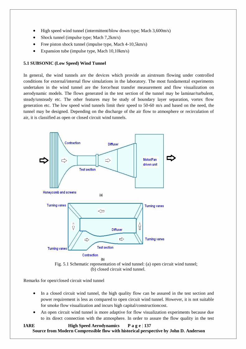
IARE High Speed Aerodynamics P a g e | 137
Source from Modern Compressible flow with historical perspective by John D. Anderson
High speed wind tunnel (intermittent/blow down type; Mach 3,600m/s)
Shock tunnel (impulse type; Mach 7,2km/s)
Free piston shock tunnel (impulse type, Mach 4-10,5km/s)
Expansion tube (impulse type, Mach 10,10km/s)
5.1 SUBSONIC (Low Speed) Wind Tunnel
In general, the wind tunnels are the devices which provide an airstream flowing under controlled
conditions for external/internal flow simulations in the laboratory. The most fundamental experiments
undertaken in the wind tunnel are the force/heat transfer measurement and flow visualization on
aerodynamic models. The flows generated in the test section of the tunnel may be laminar/turbulent,
steady/unsteady etc. The other features may be study of boundary layer separation, vortex flow
generation etc. The low speed wind tunnels limit their speed to 50-60 m/s and based on the need, the
tunnel may be designed. Depending on the discharge of the air flow to atmosphere or recirculation of
air, it is classified as open or closed circuit wind tunnels.
Fig. 5.1 Schematic representation of wind tunnel: (a) open circuit wind tunnel; (b) closed circuit wind tunnel.
Remarks for open/closed circuit wind tunnel
In a closed circuit wind tunnel, the high quality flow can be assured in the test section and
power requirement is less as compared to open circuit wind tunnel. However, it is not suitable
for smoke flow visualization and incurs high capital/constructioncost.
An open circuit wind tunnel is more adaptive for flow visualization experiments because due
to its direct connection with the atmosphere. In order to assure the flow quality in the test
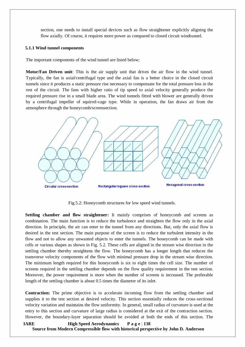
IARE High Speed Aerodynamics P a g e | 138
Source from Modern Compressible flow with historical perspective by John D. Anderson
section, one needs to install special devices such as flow straightener explicitly aligning the
flow axially. Of course, it requires more power as compared to closed circuit windtunnel.
5.1.1 Wind tunnel components
The important components of the wind tunnel are listed below;
Motor/Fan Driven unit: This is the air supply unit that drives the air flow in the wind tunnel.
Typically, the fan is axial/centrifugal type and the axial fan is a better choice in the closed circuit
tunnels since it produces a static pressure rise necessary to compensate for the total pressure loss in the
rest of the circuit. The fans with higher ratio of tip speed to axial velocity generally produce the
required pressure rise in a small blade area. The wind tunnels fitted with blower are generally driven
by a centrifugal impeller of squirrel-cage type. While in operation, the fan draws air from the
atmosphere through the honeycomb/screensection.
Fig.5.2: Honeycomb structures for low speed wind tunnels.
Settling chamber and flow straightener: It mainly comprises of honeycomb and screens as
combination. The main function is to reduce the turbulence and straighten the flow only in the axial
direction. In principle, the air can enter to the tunnel from any directions. But, only the axial flow is
desired in the test section. The main purpose of the screen is to reduce the turbulent intensity in the
flow and not to allow any unwanted objects to enter the tunnels. The honeycomb can be made with
cells or various shapes as shown in Fig. 5.2. These cells are aligned in the stream wise direction in the
settling chamber thereby straightens the flow. The honeycomb has a longer length that reduces the
transverse velocity components of the flow with minimal pressure drop in the stream wise direction.
The minimum length required for this honeycomb is six to eight times the cell size. The number of
screens required in the settling chamber depends on the flow quality requirement in the test section.
Moreover, the power requirement is more when the number of screens is increased. The preferable
length of the settling chamber is about 0.5 times the diameter of its inlet.
Contraction: The prime objective is to accelerate incoming flow from the settling chamber and
supplies it to the test section at desired velocity. This section essentially reduces the cross-sectional
velocity variation and maintains the flow uniformity. In general, small radius of curvature is used at the
entry to this section and curvature of large radius is considered at the exit of the contraction section.
However, the boundary-layer separation should be avoided at both the ends of this section. The
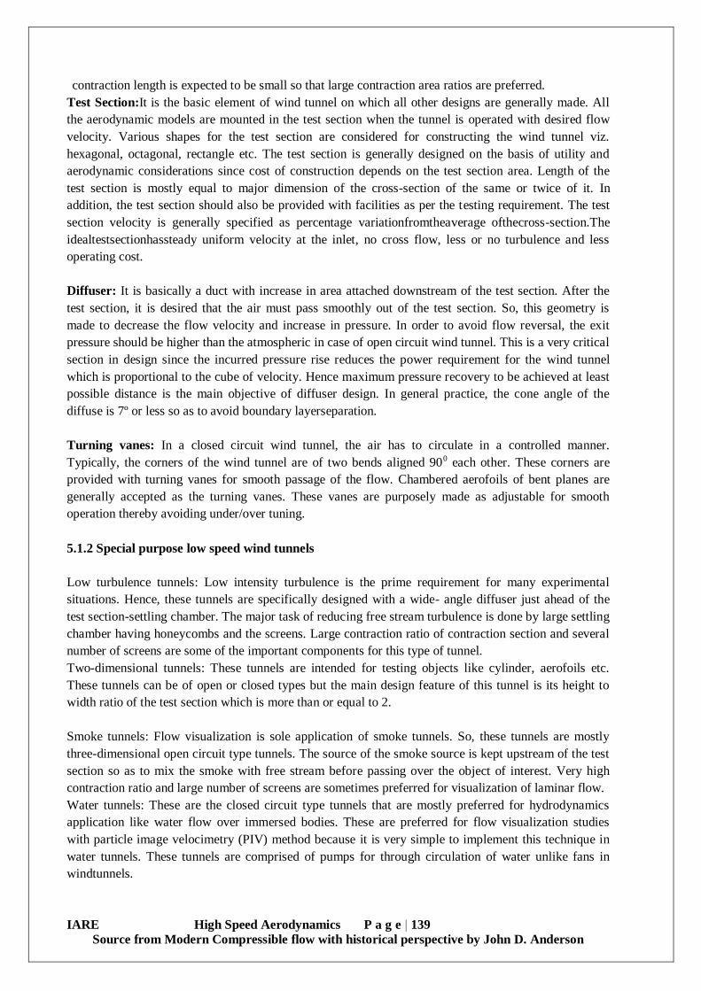
IARE High Speed Aerodynamics P a g e | 139
Source from Modern Compressible flow with historical perspective by John D. Anderson
contraction length is expected to be small so that large contraction area ratios are preferred.
Test Section:It is the basic element of wind tunnel on which all other designs are generally made. All
the aerodynamic models are mounted in the test section when the tunnel is operated with desired flow
velocity. Various shapes for the test section are considered for constructing the wind tunnel viz.
hexagonal, octagonal, rectangle etc. The test section is generally designed on the basis of utility and
aerodynamic considerations since cost of construction depends on the test section area. Length of the
test section is mostly equal to major dimension of the cross-section of the same or twice of it. In
addition, the test section should also be provided with facilities as per the testing requirement. The test
section velocity is generally specified as percentage variationfromtheaverage ofthecross-section.The
idealtestsectionhassteady uniform velocity at the inlet, no cross flow, less or no turbulence and less
operating cost.
Diffuser: It is basically a duct with increase in area attached downstream of the test section. After the
test section, it is desired that the air must pass smoothly out of the test section. So, this geometry is
made to decrease the flow velocity and increase in pressure. In order to avoid flow reversal, the exit
pressure should be higher than the atmospheric in case of open circuit wind tunnel. This is a very critical
section in design since the incurred pressure rise reduces the power requirement for the wind tunnel
which is proportional to the cube of velocity. Hence maximum pressure recovery to be achieved at least
possible distance is the main objective of diffuser design. In general practice, the cone angle of the
diffuse is 7º or less so as to avoid boundary layerseparation.
Turning vanes: In a closed circuit wind tunnel, the air has to circulate in a controlled manner.
Typically, the corners of the wind tunnel are of two bends aligned 900 each other. These corners are
provided with turning vanes for smooth passage of the flow. Chambered aerofoils of bent planes are
generally accepted as the turning vanes. These vanes are purposely made as adjustable for smooth
operation thereby avoiding under/over tuning.
5.1.2 Special purpose low speed wind tunnels
Low turbulence tunnels: Low intensity turbulence is the prime requirement for many experimental
situations. Hence, these tunnels are specifically designed with a wide- angle diffuser just ahead of the
test section-settling chamber. The major task of reducing free stream turbulence is done by large settling
chamber having honeycombs and the screens. Large contraction ratio of contraction section and several
number of screens are some of the important components for this type of tunnel.
Two-dimensional tunnels: These tunnels are intended for testing objects like cylinder, aerofoils etc.
These tunnels can be of open or closed types but the main design feature of this tunnel is its height to
width ratio of the test section which is more than or equal to 2.
Smoke tunnels: Flow visualization is sole application of smoke tunnels. So, these tunnels are mostly
three-dimensional open circuit type tunnels. The source of the smoke source is kept upstream of the test
section so as to mix the smoke with free stream before passing over the object of interest. Very high
contraction ratio and large number of screens are sometimes preferred for visualization of laminar flow.
Water tunnels: These are the closed circuit type tunnels that are mostly preferred for hydrodynamics
application like water flow over immersed bodies. These are preferred for flow visualization studies
with particle image velocimetry (PIV) method because it is very simple to implement this technique in
water tunnels. These tunnels are comprised of pumps for through circulation of water unlike fans in
windtunnels.

IARE High Speed Aerodynamics P a g e | 140
Source from Modern Compressible flow with historical perspective by John D. Anderson
5.2 High Speed (supersonic) Wind Tunnel
Experimental facilities for supersonic and hypersonic flow regimes are different from those used at
subsonic speeds. In supersonic flows, the interest lies in simulating flow Reynolds number and the
Mach numbers in the test section of the tunnel. In addition to these parameters, the total energy content
(i.e. enthalpy) of the flow also becomes important at hypersonic speeds. The wind tunnels used in the
Mach number range 1 to 5arecalledassupersonictunnelswhilethetunnelsusedforhigherMachnumbers(>5)
are called as hypersonic tunnels.
The high speed tunnels can be of open/closed circuit type. The open circuit wind tunnel takes the air
from atmosphere and rejects them to a vacuum chamber. In contrast, the same air is re-circulated in a
closed circuit wind tunnel. In the case of subsonic wind tunnels, experiments can be performed by
running the tunnel continuously. But, when the velocity of air in the test section increases, the power
requirement becomes very high because it is proportional to the cube of the velocity. Thus, in many
cases, it is preferred to run high speed wind tunnels for a short duration and gather all the experimental
data in this short time period (~1-5s). So, such types of tunnels are called as blow down tunnels. These
tunnels operate intermittently using high pressure tanks and/or vacuumtanks.
5.2.1 Blow down wind Tunnel (Open circuit type)
The high pressure chamber, vacuum section, nozzle and test section are few important
componentsofablowdownwindtunnel.TheschematicdiagramisshowninFig.5.3. Since, the air from the
high pressure chamber flows towards the vacuum section, it is referred as pressure-vacuum tunnel. First,
the air is taken from the atmosphere and after compression; it is stored in a tank. Simultaneously, the
low pressure section is evacuated by a vacuum pump. Pressure regulator controls the air flow from
reservoir to the settling chamber during the actual experiment and maintains the desired constant
pressure. The nozzle expands the flow by increasing velocity and decreasing pressure and provides
desired Mach number in the test section. The high speed air encounters deceleration while passing
through the second throat.
These blow down tunnels are inherent intermittent tunnels but bear many advantages over
continuous wind tunnels such as high Mach capability (up to 4), easy tunnel starting, large size test
section, lower construction/operating costs, superior design for propulsion experiments and smoke
visualization.
The limitations of the blow down tunnels are requirement of faster data acquisition system, noisy
operation and necessity of pressure regulator valves. The blow down tunnel can be of different types
based on the driving pressure difference is achieved. In one such tunnel, air expands from high pressure
to the atmospheric pressure where low pressure chamber is excluded (intermittent blow down tunnel). In
other cases, the atmospheric air can expand up to a very low vacuum (intermittent in-draft wind tunnel).
Depending on the requirement of Mach number in the test section, the tunnel is chosen accordingly.
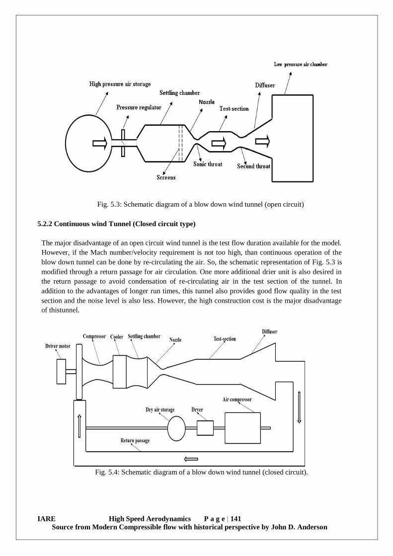
IARE High Speed Aerodynamics P a g e | 141
Source from Modern Compressible flow with historical perspective by John D. Anderson
Fig. 5.3: Schematic diagram of a blow down wind tunnel (open circuit)
5.2.2 Continuous wind Tunnel (Closed circuit type)
The major disadvantage of an open circuit wind tunnel is the test flow duration available for the model.
However, if the Mach number/velocity requirement is not too high, than continuous operation of the
blow down tunnel can be done by re-circulating the air. So, the schematic representation of Fig. 5.3 is
modified through a return passage for air circulation. One more additional drier unit is also desired in
the return passage to avoid condensation of re-circulating air in the test section of the tunnel. In
addition to the advantages of longer run times, this tunnel also provides good flow quality in the test
section and the noise level is also less. However, the high construction cost is the major disadvantage
of thistunnel.
Fig. 5.4: Schematic diagram of a blow down wind tunnel (closed circuit).

IARE High Speed Aerodynamics P a g e | 142
Source from Modern Compressible flow with historical perspective by John D. Anderson
5.3 Impulse-Type Tunnels
The conventional hypersonic wind tunnels face the challenges of simulating re-entry flight
phenomena, long range ballistic missile test conditions that occurs at very altitudes. Since, the
temperature can rise up to 10000K, there will be dissociations, chemical reactions as well. Hence, such
investigations need real gas simulation conditions and it is almost impossible to achieve them in
conventional hypersonic wind tunnels. So, the concept of impulse type aerodynamic facilities is
introduced where it is desired to produce low density and high enthalpy flows for a very short duration
(~ few milliseconds).
Expansion and shock tunnels are the typical aerodynamic testing facilities with a specific interest
in high speeds and high temperature testing. Shock tunnels use steady flow nozzle expansion whereas
expansion tunnels use unsteady expansion with higher enthalpy/thermal energy. In both cases the gases
are compressed and heated until the gases are released, expanding rapidly down the expansion
chamber. The tunnels reach speeds from Mach numbers ranging 3 to 30, thus creating testing
conditions similar to that of very high altitudes.
Shock Tunnel: It consists of two major parts, the shock tube and the wind tunnel portion. The general
schematic layout of the shock tunnel, consisting of shock tube and wind tunnel section, is shown in
Fig. 5.5. The shock tube portion consists of a constant area tube separated by a diaphragm (generally,
metal) into regions of high and low pressures. High and low pressure regions are called ‘driver tube’
and ‘driven tube’ respectively. The shock tube works on the principle of using a high-pressure gas in
the driver tube to set up a shock wave, which propagates into the low pressure gas in the driven tube at
the instant of diaphragm rupture. The propagating shock wave compresses and heats the low-pressure
test gas in the driven tube to a high pressure and temperature, and also imparts the test gas a high
kinetic energy, with which it starts moving at a supersonic Mach number behind the propagating shock
wave. This shock wave ideally travels through the driven section at a constant velocity, and there
exists a region of steady supersonic flow of high temperature and pressure between the moving
driver/driven gas interface and the shockwave.
The wind tunnel portion of the shock tunnel consists of a hypersonic nozzle that is attached to
the driven end of the shock tube, a test section at the exit of the nozzle where the measurements are
carried out, and a dump tank portion to accommodate the gas. The shocked high pressure/temperature
gas from the shock tube is then expanded through the hypersonic nozzle to the desired Mach number
and velocity in the tunnel test section.
Fig.5.5: Schematic representation of a shock tunnel.

IARE High Speed Aerodynamics P a g e | 143
Source from Modern Compressible flow with historical perspective by John D. Anderson
The ability of the shock tube portion of the hypersonic shock tunnel to heat the test gas to the
conditions encountered in hypersonic flight makes it an attractive tool for hypersonic flow research.
The test flow duration in a shock tunnel is in the range of1ms.
5.4 Free Piston Shock Tunnel
In a typical shock tunnel, the high pressure in the driver section is achieved by filling the tube from a
high pressure gas cylinder. Thus, the driver gas is normally at room temperature. In the low density
environment, it is likely that condensation may arise in the test section. So, many test facilities involve
preheating the driver gas. One of them is to use a free piston driver to operate the shock tunnel. Here,
the compression tube is filled with a driver gas (typically at atmospheric pressure) and is coupled to
the driven section of low pressure region at one end and to a reservoir at very high pressure air (~100
bar). In this way, the piston separates the reservoir from the compression tube. When the piston is
released for firing, it accelerates in the compression tube by acquiring the energy of expanding
reservoir gas. The piston then approaches down to the compression tube and transfers all its energy to
the driver gas. In this way, both temperature and pressure can be increased due to adiabatic
compression mechanism. In a typical facility, the pressure up 900 bar and temperature of 4500K can
be achieved. At this high pressure the primary diaphragm ruptures and shock tube flow is initiated in
the similar manner as discussed earlier. In a well designed free piston shock tunnel, it is possible to
achieve test flow duration up to2ms.
Fig. 5.6: Schematic diagram of a free piston shock tunnel.
5.5 Detonation-driven shock tunnels (tube)
The detonation-driven shock tube, first proposed by Bird,3 has been studied by several investigators. In
a detonation-driven shock tube or shock tunnel, the conventional driver is replaced by a detonation
section filled with a detonable gas mixture. Typically, an oxyhydrogen mixture is used as the driver gas
with helium or argon dilution. Helium dilution raises the sonic speed in the driver gas and also
somewhat reduces the danger associated with premature detonation.
A. Upstream Mode
Two modes of operation are possible. In the upstream-or backward propagation mode, the ignition
source is just upstream of the primary diaphragm between the detonation and driven sections. In this
case, the detonation wave propagates upstream. The corresponding wave diagram is shown in Fig. 5.7.

IARE High Speed Aerodynamics P a g e | 144
Source from Modern Compressible flow with historical perspective by John D. Anderson
Fig 5.7: Principle of an upstream detonation-driven shock tunnel.
Direct initiation leads to a stable detonation wave where the products are at high temperature and
pressure. The pressure rise following the detonation wave is constant, but the momentum imparted to
the driver gas by the detonation wave is directed upstream, that is, opposite to the main flow. This leads
to a reduction of the effective driver performance. Shortly after initiation, the main diaphragm opens
and the burnt products exhaust into the low-pressure section, driving the incident shock that compresses
and heats the test gas. A Taylor expansion immediately follows the detonation wave, decelerating the
burnt gas to zero velocity along the characteristic labeled e in Fig. 5.7. This is common with the usual
Taylor expansion as it develops behind a detonation wave starting in a closed- end tube to match the
boundary conditions there. After the main diaphragm rupture, the shock tube expansion develops, which
merges with the Taylor Expansion. It follows that for the upstream mode, the effective driver condition
for the shock tube process is not achieved immediately behind the detonation wave but along the
characteristic e where the flow velocity is zero.
The upstream running detonation was creates a tremendous pressure, of as much as 200 times the initial
filling pressure, as it reflects from the end wall of the driver. Indeed, a shock tube was damaged because
of this over pressure. To avoid or at least reduce the mechanical loading of the facility because of wave
reflection, Yu proposed installing a damping section upstream of the detonation section. This damping
section is filled with nitrogen at a relatively low pressure of approximately 3-7 kPa. Between the
damping and detonation section is a thin plastic diaphragm. The detonation wave enters the damping
section without significant reflection. There it extinguishes and propagates as a shock toward the end
wall, where the pressure behind this shock is much smaller than that behind the detonation wave. With
this technique, the mechanical loading on the facility is reduced acceptably.
The second advantage of the damping section lies in the increase of duration of constant driver
properties. Without a damping section, the detonation wave reflects at the driver end wall and
propagates downstream as a shock. If a damping tube is attached to the driver, a rarefaction wave is
generated at the diaphragm station between the driver and damping section. The tail of this rarefaction
wave travels towards slower than the reflected shock, the damping section yields a longer flow duration
of constant driver conditions.
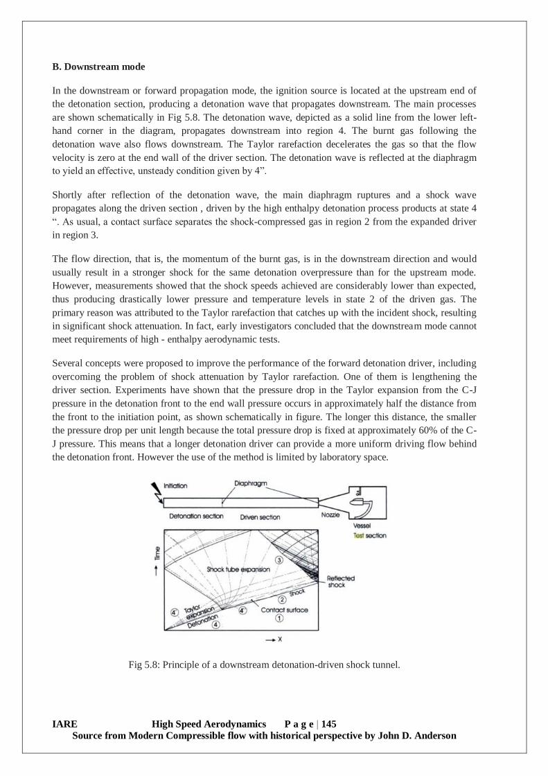
IARE High Speed Aerodynamics P a g e | 145
Source from Modern Compressible flow with historical perspective by John D. Anderson
B. Downstream mode
In the downstream or forward propagation mode, the ignition source is located at the upstream end of
the detonation section, producing a detonation wave that propagates downstream. The main processes
are shown schematically in Fig 5.8. The detonation wave, depicted as a solid line from the lower left-
hand corner in the diagram, propagates downstream into region 4. The burnt gas following the
detonation wave also flows downstream. The Taylor rarefaction decelerates the gas so that the flow
velocity is zero at the end wall of the driver section. The detonation wave is reflected at the diaphragm
to yield an effective, unsteady condition given by 4”.
Shortly after reflection of the detonation wave, the main diaphragm ruptures and a shock wave
propagates along the driven section , driven by the high enthalpy detonation process products at state 4
“. As usual, a contact surface separates the shock-compressed gas in region 2 from the expanded driver
in region 3.
The flow direction, that is, the momentum of the burnt gas, is in the downstream direction and would
usually result in a stronger shock for the same detonation overpressure than for the upstream mode.
However, measurements showed that the shock speeds achieved are considerably lower than expected,
thus producing drastically lower pressure and temperature levels in state 2 of the driven gas. The
primary reason was attributed to the Taylor rarefaction that catches up with the incident shock, resulting
in significant shock attenuation. In fact, early investigators concluded that the downstream mode cannot
meet requirements of high - enthalpy aerodynamic tests.
Several concepts were proposed to improve the performance of the forward detonation driver, including
overcoming the problem of shock attenuation by Taylor rarefaction. One of them is lengthening the
driver section. Experiments have shown that the pressure drop in the Taylor expansion from the C-J
pressure in the detonation front to the end wall pressure occurs in approximately half the distance from
the front to the initiation point, as shown schematically in figure. The longer this distance, the smaller
the pressure drop per unit length because the total pressure drop is fixed at approximately 60% of the C-
J pressure. This means that a longer detonation driver can provide a more uniform driving flow behind
the detonation front. However the use of the method is limited by laboratory space.
Fig 5.8: Principle of a downstream detonation-driven shock tunnel.

IARE High Speed Aerodynamics P a g e | 146
Source from Modern Compressible flow with historical perspective by John D. Anderson
Fig 5.9 A simple model for the distribution of detonation wave along the length of a detonation tube.
5.6 Expansion Tunnel
It uses a dual-diaphragm system where the diaphragms act as rupture discs, or a pressure relief.
The tunnel is separated into three sections: driver, driven, and acceleration as shown in Fig. 5.10.
The driver section can be fired either by a high pressure gas or by a free piston driver. The driven
section is filled with a lower pressure test gas. The acceleration section is filled with an even
lower pressurized test gas. Each section is divided by a diaphragm, which is meant to be ruptured
in sequence causing the first diaphragm to rupture, mixing and expanding the driver and the
driven. When the shock wave hits the second diaphragm, it ruptures casing the two gases to mix
with the acceleration and expand down the enclosed test section. In this way, the flow of the test
flow can be increased for hypervelocity conditions. However, the operation time is approximately
250µs.
Fig. 51.0: Schematic diagram of an expansion tube.

IARE High Speed Aerodynamics P a g e | 147
Source from Modern Compressible flow with historical perspective by John D. Anderson
5.7 Flow Visualization Techniques for Compressible Flows
5.7.1 Introduction
Flow visualization is carried out to understand the physics of the flow in detail. Understanding of the
flow provides excellent description which in turn helps to calculate flow properties for many problems
of practical interests in both compressible subsonic and supersonic flow regimes. Flow visualization can
be of interest for various problems. Since air is transparent, thus their flow patterns are invisible to us
without incorporating special techniques to visualize the same. Therefore the present section deals with
some important flow visualization techniques.
5.7.2 Interferometer
The interferometer which is an optical method is specifically suited for qualitative determination of the
density field of high speed flows. From the theory of light, we know that when light travels through a
gas the velocity of propagation is affected by the physical properties of the gas. Principle of working of
the interferometer is based on this fact.
Figure 5.11 shows the essential features of the Mach-Zhender Interferometer. Light emitted from the
source is allowed to pass through the lens L1 which makes the light rays parallel with each other. These
parallel light beams are then passed through a monochromatic filter. The path of the light wave is then
made by two ways as M1-M2-M4 and M1-M3-M4 in the way to fall on the screen as shown in Fig.5.11.
Here M represents mirror shown in same figure. These two paths are possible due to half silvered mirror
M1 which divides a light beam into two beams. These two beams travel same distance in their
respective paths before recombining at lens L2 and getting projected on the screen. Although the length
of travel for both the beams is same, however the medium of travel is necessarily different since one
beam which travels via M1-M3-M4 path actually encounters room air whereas the other beam travelling
through M1-M2-M4 passes through the test section. For the situation without any flow through the test
section, both the rays face similar medium and fall on the screen as a single ray after combining. Thus a
screen gets illuminated by a uniform patch of light. However, the situation changes with in the presence
of flow in the test section where density change is encountered by one ray in the presence of shock. This
increased density retards the beam passing through the test section and hence creates phase difference
between the two beams. If this phase difference is λ/2 where λ is wave length, then two rays mark
contrast spots on the screen. Therefore, we can observe dark and white bands on the screen for
appreciable difference in the density.
Fig 5.11 Mach-Zhender Interferometer.
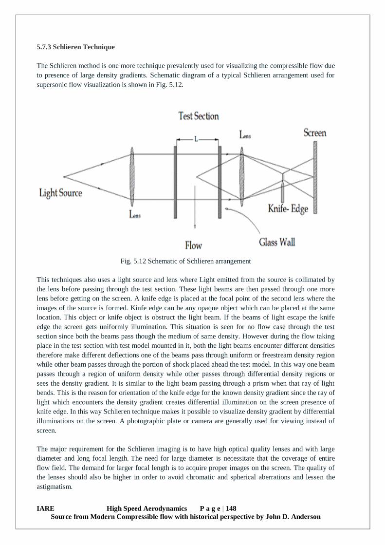
IARE High Speed Aerodynamics P a g e | 148
Source from Modern Compressible flow with historical perspective by John D. Anderson
5.7.3 Schlieren Technique
The Schlieren method is one more technique prevalently used for visualizing the compressible flow due
to presence of large density gradients. Schematic diagram of a typical Schlieren arrangement used for
supersonic flow visualization is shown in Fig. 5.12.
Fig. 5.12 Schematic of Schlieren arrangement
This techniques also uses a light source and lens where Light emitted from the source is collimated by
the lens before passing through the test section. These light beams are then passed through one more
lens before getting on the screen. A knife edge is placed at the focal point of the second lens where the
images of the source is formed. Kinfe edge can be any opaque object which can be placed at the same
location. This object or knife object is obstruct the light beam. If the beams of light escape the knife
edge the screen gets uniformly illumination. This situation is seen for no flow case through the test
section since both the beams pass though the medium of same density. However during the flow taking
place in the test section with test model mounted in it, both the light beams encounter different densities
therefore make different deflections one of the beams pass through uniform or freestream density region
while other beam passes through the portion of shock placed ahead the test model. In this way one beam
passes through a region of uniform density while other passes through differential density regions or
sees the density gradient. It is similar to the light beam passing through a prism when that ray of light
bends. This is the reason for orientation of the knife edge for the known density gradient since the ray of
light which encounters the density gradient creates differential illumination on the screen presence of
knife edge. In this way Schlieren technique makes it possible to visualize density gradient by differential
illuminations on the screen. A photographic plate or camera are generally used for viewing instead of
screen.
The major requirement for the Schlieren imaging is to have high optical quality lenses and with large
diameter and long focal length. The need for large diameter is necessitate that the coverage of entire
flow field. The demand for larger focal length is to acquire proper images on the screen. The quality of
the lenses should also be higher in order to avoid chromatic and spherical aberrations and lessen the
astigmatism.

IARE High Speed Aerodynamics P a g e | 149
Source from Modern Compressible flow with historical perspective by John D. Anderson
It has been observed that is difficult to visualize images using this technique for very large cross section
wind tunnels due to unavailability of high optical quality and diameter of lenses. The cost of such lenses
is the major concern is such cases. Use of concave mirrors is the immediate remedy on such situations.
This is due to the fact that these lenses are easy to fabricate and also to correct during the experimental
setting. The minimum optical quality is implicit in these lenses. The Schlieren arrangement with such
low cost lenses is as shown in Fig 5.13.
Fig. 5.13. Schematic of twin Schlieren arrangement
5.7.4 Planar Laser Induced Fluorescence (PLIF)
Optical techniques are considered for flow visualization, Planar Laser Induced Fluorescence (PLIF) is
among such methods. This lased based technique is popular due to its abilities like remote controlling,
precise prediction and non-intrusive. In this technique, a laser sheet is used to illuminate the flow and
captures the fluorescence. Radicals which are most active species on the flow are chosen to track in this
technique using the laser sheet to excite the species and hence to emitted the fluorescence which is
captured on charge-coupled device (ICCD) camera.
A basic arrangement of PLIF is illustrated below in Fig 5.14. Consider a burner whose fluorescence is
expected to capture. Therefore a laser beam passes through a cylindrical lens to convert it into a thin
laser sheet. This laser sheet passes through the flame produced by a flat flame burner and excites the OH
radical which inturn causes fluorescence. This fluorescence signal is then acquired in the camera in the
form of the images. The images captured in the ICCD can be further considered for processing.

IARE High Speed Aerodynamics P a g e | 150
Source from Modern Compressible flow with historical perspective by John D. Anderson
Fig 5.14 Basic Arrangement of PLIF
Disadvantages of PLIF: The major disadvantage is the quenching of the fluorescence at high pressure
conditions due to high number of collisions of the molecules.