AAS 03-261

GENERALIZED GRADIENT SEARCH AND NEWTON’S

METHODS FOR MULTILINEAR ALGEBRA ROOT-SOLVING AND

OPTIMIZATION APPLICATIONS

James D. Turner, Ph.D

ABSTRACTA standard problem in optimization involves solving for the roots of nonlinear functions defined by f(x) = 0, where x is the unknown variable. Classical algorithms consist of first-order gradient search and Newton-Raphson methods. This paper generalizes the Newton-Raphson Method for multilinear algebra root-finding problems by introducing a non-iterative multilinear reversion of series approximation. The series solution is made possible by introducing an artificial independent variable through an embedding process. Automatic Differentiation techniques are defined for evaluating the generalized iteration algorithms. Operator-overloading strategies use hidden tools for redefining the computers intrinsic mathematical operators and library functions for building high-order sensitivity models. Exact partial derivatives are computed for first though fourth order, where the numerical results are accurate to the working precision of the machine. The analyst is completely freed from having to build, code, and validate partial derivative models. Accelerated convergence rates are demonstrated for scalar and vector root-solving problems. An integrated generalized gradient search and Newton-Raphson algorithm is presented for rapidly optimizing the very challenging classical Rosenbrock’s Banana function. The integration of generalized algorithms and automatic differentiation is expected to have broad potential for impacting the design and use of mathematical programming tools for knowledge discovery applications in science and engineering.

INTRODUCTIONMany applications in engineering, science, and mathematics require solutions for equations of the

form , where x is the unknown root of the equation. Given an initial guess, x, the classical Newton-Raphson strategy seeks a correction, , by assuming that the function can be expanded as the following Taylor series

(1)where denotes the derivative with respect to x. Eliminating terms of O(2) and higher, provides the following correction model for the improved root guess given by x:= x + . Under well-defined conditions for f(x) and its derivatives the solution accuracy is improved by repeating the procedure until |f(x)| < , where is a prescribed solution tolerance. Even though each iteration doubles the number of accurate digits, many algorithms have been proposed for accelerating the convergence rate15. All of these algorithms retain O(2) and higher terms in Eq. (1), and generate higher-order approximations

1

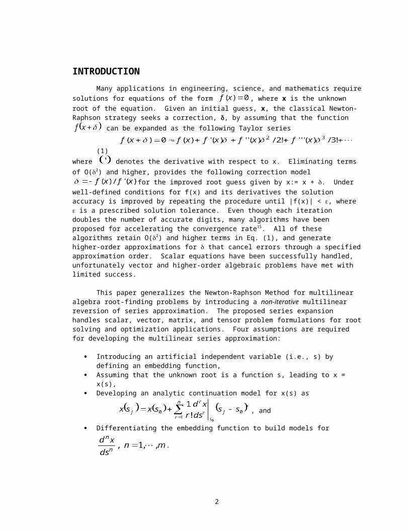
for that cancel errors through a specified approximation order. Scalar equations have been successfully handled, unfortunately vector and higher-order algebraic problems have met with limited success.

This paper generalizes the Newton-Raphson Method for multilinear algebra root-finding problems by introducing a non-iterative multilinear reversion of series approximation. The proposed series expansion handles scalar, vector, matrix, and tensor problem formulations for root solving and optimization applications. Four assumptions are required for developing the multilinear series approximation:

Introducing an artificial independent variable (i.e., s) by defining an embedding function, Assuming that the unknown root is a function s, leading to x = x(s), Developing an analytic continuation model for x(s) as

, and

Differentiating the embedding function to build models for .

The Multilinear Problem

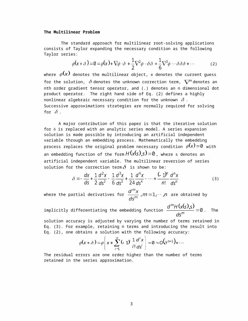
The standard approach for multilinear root-solving applications consists of Taylor expanding the necessary condition as the following Taylor series:

(2)

where denotes the multilinear object, x denotes the current guess for the solution, denotes the unknown correction term, denotes an nth order gradient tensor operator, and (.) denotes an n dimensional dot product operator. The right hand side of Eq. (2) defines a highly nonlinear algebraic necessary condition for the unknown . Successive approximations strategies are normally required for solving for .

A major contribution of this paper is that the iterative solution for is replaced with an analytic series model. A series expansion solution is made possible by introducing an artificial independent variable through an embedding process. Mathematically the embedding process replaces the original problem necessary condition with an embedding function of the form , where s denotes an artificial independent variable. The multilinear reversion of series solution for the correction term is shown to be:

(3)

where the partial derivatives for are obtained by implicitly differentiating the

embedding function . The solution accuracy is adjusted by varying the number of

terms retained in Eq. (3). For example, retaining n terms and introducing the result into Eq. (2), one obtains a solution with the following accuracy:

The residual errors are one order higher than the number of terms retained in the series approximation.

2

Computational Issues for Generating High-Order Partial Derivative Models

High-order partial derivative models are required for successfully applying the multilinear reversion of series solution. To this end, both theoretical and computational issues are addressed. The theoretical issue is addressed by introducing a coordinate embedding strategy, which provides an embedding function that is processed for building analytic partial derivative models. The computational issue is addressed by introducing Automatic Differentiation (AD) techniques. These tools enable the automatic derivation and evaluation of arbitrarily complex partial derivative models. For all derivative orders, the AD-generated models are accurate to the working precision of the machine. The analyst is completely freed from having to build, code, and validate partial derivative models.

Object-Oriented Kernel Capabilities. Object-oriented language features and operator overloading computational capabilities provide the foundation for all AD technologies presented in this paper. An Object-Oriented Coordinate Embedding Method (OCEA) is introduced for providing a conceptual framework for developing AD-based application toolkits. Arbitrarily complex and large problem sizes are easily handled. OCEA data structures are ideally suited for computing the rates appearing in multilinear reversion of series algorithms. The proposed generalized gradient search/Newton-Raphson methods only become practical when linked to automated capabilities for computing high-order partial derivative models. The integration of multilinear reversion of series and AD tools are expected to impact both real-world applications as well as problems on the frontiers of computational science and engineering.

HISTORICAL BACKGROUND

Sir Isaac Newton (1643-1727) presented a new algorithm for solving a polynomial equation in 16691, where an initial guess plus an assumed small correction is used to transform the polynomial function. By linearizing the transformed polynomial for the small correction term and repeating the process several times, he effectively solved the polynomial equation. Newton did not define a derivative for the polynomial as part of his algorithm. The notion of a derivative was introduced into what has become known as Newton’s method in 1690 by Joseph Raphson (1678-1715)2. By including the derivative the method is also known as the Newton-Raphson method, where the iteration formula is given by

. Given a starting guess for the root x0, the limit of the sequence for x1, x2, …, xn converges to the desired root under well defined conditions for f(x) and its derivatives. For a convergent sequence for x1, x2, …, xn, the number of accurate digits double at each stage of the iteration.

Accelerated Convergence for Scalar Newton-Raphson Problems. Many Authors have proposed methods to accelerate the convergence rate for Newton’s Method. For example, the astronomer E. Halley (1656-1743) in 1694 developed the second-order expansion

where the number of accurate digits triple at each stage of the iteration2. Householder3 later developed the general iteration formula

where p is an integer and (1/f)p denotes the derivative of order p of the inverse of the function f. Remarkably, this iteration has a convergence rate of order (p+2). Consequently, when p=0 the algorithm has quadratic convergence and reproduces the performance of the original Newton’s Method, and when p=1 the algorithm has cubical convergence that reproduces Halley’s results. Several ad-hoc methods have

3

been proposed for extending the accelerated convergence rates for scalar equations through eighth order15. Extensions for vector systems have been limited to cubic convergence rates using Chebyshev’s method. On the Link Between Newton’s And Reversion of Series Methods. All versions of the Newton-Raphson method and the classical reversion of series algorithm are shown to be identical. The key step involves introducing an embedding parameter that transforms the inequality constraint form of the Newton’s method necessary condition into an equality constraint. To this end, recall that the Eq. (1) is defined by the following nonlinear inequality constraint:

where is the unknown. This nth order polynomial equation is difficult to solve and multiple solutions can exist. The solution process is simplified by transforming the inequality constraint into an equality constraint by introducing an artificial embedding parameter, s, leading to:

This equation defines a functional relationship of the form , where the desired solution for is recovered when s = 0. Classically, the solution for is obtained by reverting the series, yielding an equation of the form . Retaining fifth order terms in the approximation for , and using the symbol manipulating computer algebra system MACSYMA, a classical series reversion method yields:

Introducing s = 0 into the equation above (i.e., ), one can identify all previously reported algorithms for accelerated Newton-Raphson algorithms for scalar equations, as follows:

where the convergence rate is defined by n+1 and n is defined by the expression . Extensions for arbitrary order are easily formulated. Unfortunately, the multilinear generalizations of these approximations are not immediately obvious. The success of the embedding strategy for scalar equations, however, suggests that an embedding strategy can be equally effective for multilinear problems.

Generalized Newton Method for Non-Scalar Equation. A multilinear reversion of series solution is developed for Newton’s Method. As in the scalar equation case, an artificial independent variable, s, is introduced into the original problem, which allows a series expansion model to be developed. The previously successful scalar function embedding approach, however, does not extend to multilinear systems because many simultaneous constraint conditions must be satisfied. A new embedding strategy is required for defining a scalar embedding parameter so that x = x(s).

EMBEDDING / REVERSION OF SERIES ALGORITHM

The original root-solving problem is embedded into a space of higher dimension, by introducing an artificial independent variable. To this end, the original necessary condition root is redefined as the following parameter embedding problem10:

(4)

4

where s is scalar embedding parameter, xg is the starting guess, and x = x(s). Like the scalar example, the embedding function transforms an inequality constraint into an equality constraint. Even though H( x(s), s) is a multilinear object, Eq.(4) is easily handled by introducing a scalar parameter. The initial and final states of the embedding function are presented in Table 1. As in the scalar case, the solution for the original problem is recovered by selecting so that the original problem necessary condition is satisfied. Specifying how x changes along the curve defined by H(x(s), s) solves the root-solving problem for H(x(s), s) = 0 as s varies from 1 to 0. The solution curve for x is known as a homotopy path10.

Table 1

EMBEDDING FUNCTION INITIAL AND FINAL STATES

Embedding Function

Evaluation Point

Embedding Function Comment

s = s0 = 1 Because (initial guess)

s = sf = 0 Original Function Returned

Series Expansion for the Root of

Along the homotopy path defined by Eq. (4) (i.e., analytic continuation path), the solution for x(s) is generated by the following Taylor series

(5)

where and denotes the starting guess for the root. Setting in Eq. (5) eliminates the artificial independent variable from the series solution and restores the original problem dimension, yielding the non-iterative reversion of series solution:

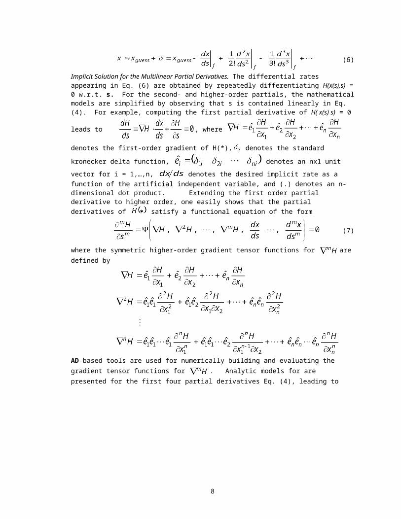
(6)

Implicit Solution for the Multilinear Partial Derivatives. The differential rates appearing in Eq. (6) are obtained by repeatedly differentiating H(x(s),s) = 0 w.r.t. s. For the second- and higher-order partials, the mathematical models are simplified by observing that s is contained linearly in Eq. (4). For example,

computing the first partial derivative of H( x(s) s) = 0 leads to , where

denotes the first-order gradient of H(*), denotes the standard

kronecker delta function, denotes an nx1 unit vector for i = 1,…,n, denotes the desired implicit rate as a function of the artificial independent variable, and (.) denotes an n-dimensional dot product. Extending the first order partial derivative to higher order, one easily shows that the partial derivatives of satisfy a functional equation of the form

(7)

where the symmetric higher-order gradient tensor functions for are defined by

5

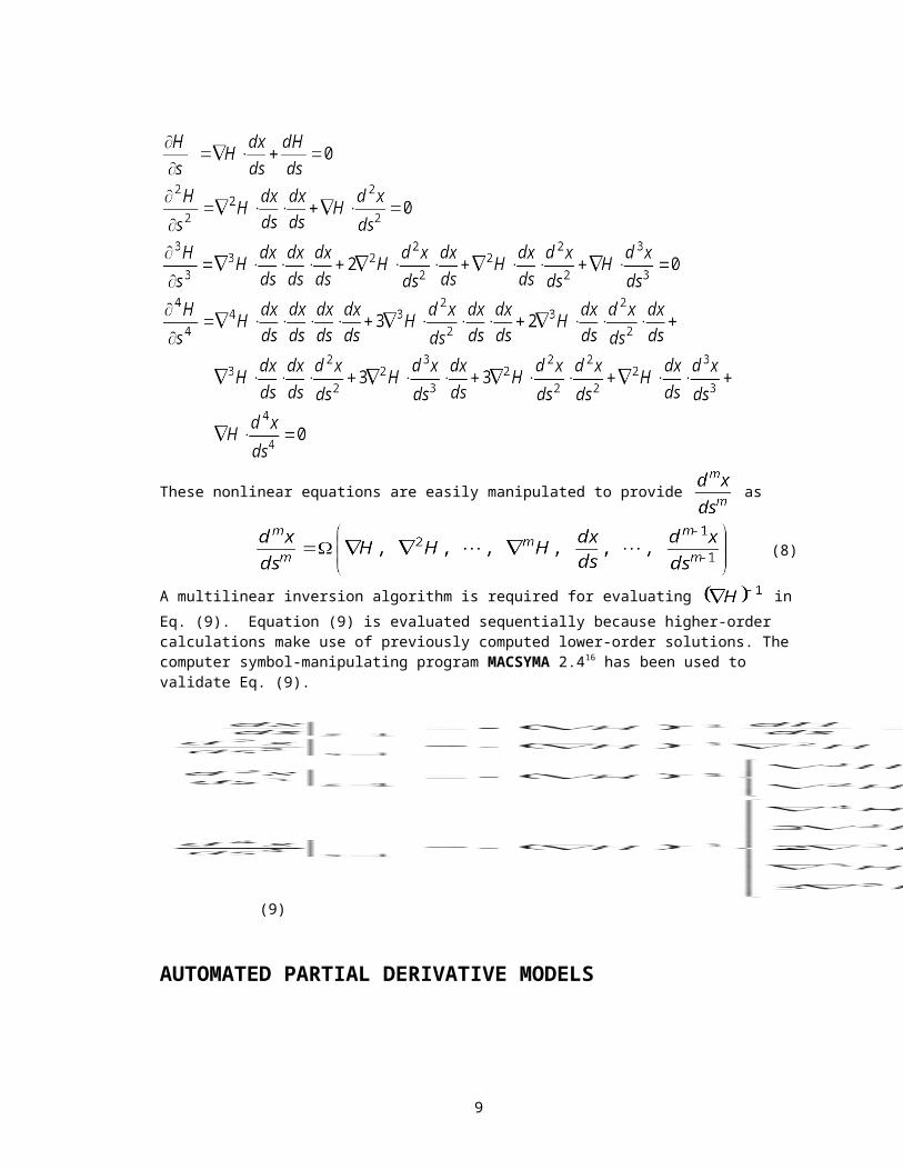
AD-based tools are used for numerically building and evaluating the gradient tensor functions for . Analytic models for are presented for the first four partial derivatives Eq. (4), leading to

These nonlinear equations are easily manipulated to provide as

(8)

A multilinear inversion algorithm is required for evaluating in Eq. (9). Equation (9) is evaluated sequentially because higher-order calculations make use of previously computed lower-order solutions. The computer symbol-manipulating program MACSYMA 2.416 has been used to validate Eq. (9).

(9)

6

AUTOMATED PARTIAL DERIVATIVE MODELS

The partial derivative models appearing in Eq. (9) are extremely complicated. Automated numerical techniques are introduced for building and evaluating these models. Research for AD methods has existed as a research topic since the 1980’s11-14. Examples of previously developed AD tools include:

ADIFOR11-12 for evaluating 1st order partials, AD018 which uses F90 operator-overloading techniques7-9 and computational graphs, ADOL-C which uses a graph-based C/C++ code for 1st order partials ADMIT-1which represents a MATLAB interface toolbox for linking different AD codes to the

MATLAB environment, AUTO_Deriv which transformations of FORTRAN codes, and OCEA for building 1st through 4th order partials in FORTRAN 90 and MACSYMA.

AD-based applications have appeared for optimization, robotics, multibody, algorithms, and molecular dynamics. A significant limitation of these tools has been that Hessian capabilities are only available for scalar objective functions and vector objective function applications are limited to Jacobians.

OCEA-Based Automated Partial Derivative Capabilities

OCEA provides a powerful language extension for engineering and scientific software development. Arbitrary order partial derivative capabilities are enabled by embedding multiple levels of the chain rule of calculus in the transformed operators and functions. The embedded chain rules build the partial derivative models on-the-fly, without analyst intervention, using hidden computational resources. The analyst uses standard programming constructs for building computer-based models: hidden operator-overloading tools build and evaluate the partial derivative models.

Arbitrarily large and complex problems are handled because OCEA exploits generalized scalar operations for all numerical calculations. Operator-overloading techniques transform the computers intrinsic operators and functions for enabling these advanced capabilities. A two-stage transformation process is employed. First, each OCEA-transformed scalar becomes an abstract compound data object, consisting of the original scalar plus hidden artificial dimensions for performing and storing the partial derivative calculations. Second, multiple levels of the chain rule of calculus are embedded in each mathematical operator and library function. An OCEA module consists of a linked set of intrinsic operators, math library functions, embedded chain rules, and composite function rules.

For the root-solving and optimization problems considered in this paper, automated tools virtually eliminate the time consuming, error prone process of modeling, coding, and verifying sensitivity calculations. Many algorithms only require the insertion of a USE Module Statement and some minor changes of variable types, including matrix operations4-6.

OCEA Algorithm

OCEA methodology is a transformational process that changes functional and partial derivative data into new forms during calculations. A single OCEA function evaluation generates exact numerical values for the function as well as hidden values for the Jacobian, and higher-order partial derivatives. All of the mathematical library functions require generalized composite function transformations for linking current calculations with all previous sensitivity calculations. Module functions support a mixed object/data type computational environment, where integer, real, double precision, complex, and OCEA data types can co-exist. The partial derivatives are extracted by utility routines as a post-processing step. Fortran 90 (F90) and Macsyma 2.4 OCEA prototype codes have been developed.

The development of an OCEA toolbox for engineering and scientific applications is addressing the following seven software issues: Defining how independent variables are transformed to OCEA form;

7

Developing derived data types for vectors, tensors, and embedded variables; Defining interface operators for supporting generalized operations; Using Module functions to hide OCEA computational resources; Defining OCEA-enhanced library routines that encode chain rule models; Providing utility routines to access the OCEA partial derivative calculations; and Developing application suites of software for solving broad classes of mathematical programming problems. Second-order OCEA models are presented for discussing each of these issues.

Data Structures. Each scalar variable is modeled as a compound data object consisting of a concatenation of the original scalar variable and its first and higher order partial derivatives. Compound data objects are created using Derived data types. The partial derivative models are not visible to the user during calculations, and can be thought of as hidden artificial dimensions for the transformed scalar variables. A significant benefit of employing hidden artificial dimensions is that the structure and computational sequencing of standard algorithms is not impacted.

For example, in the OCEA algorithm, the 1x1 scalar g has the following transformed data structure7-9:

where the transformed version of g has dimension 1x(1+m+m2). The new object consists of a concatenation of the variable and two orders of partial derivatives. Generalizations for higher dimensional versions of OCEA are obvious. Future enhancements will embed additional computational information for handling data sub-structuring information, sparse structure data, symmetry, and parallel computations.

Operator Overloading. OCEA-based AD capabilities require four mathematical elements: 1) Generalized intrinsic binary operators { +, -, *, **, / }, 2) Generalized unary functions { cos(x), sin(x), tan(x), log(x),….}, 3) Encoded multi-level chain rule implementations for all new operators and functions, and 4) Generalized composite function operators. Derived data types and interface operators7-9 manage the OCEA binary operators and unary functions. Expressing these requirements in F90, leads to 50+ Module-hidden routines for redefining the intrinsic and mathematical library functions. Operator overloading facilities manage the definitions for interface operators that allow the compiler to recognize 1) The mathematical operators or functions, and 2) The argument list data types (including user-defined data types) for automatically building links to the hidden routines at compile time.

Four factors impact the efficiency of OCEA partial derivative calculations: 1) partial derivative order, 2) exploitation of sparse structure, 3) exploitation of symmetry, and 4) level of optimization for the OCEA generalized intrinsic and mathematical functions. These topics remain active areas of continuing research. A full exploitation of all of these factors is anticipated to impact the performance of OCEA-based tools by 10-100 fold.

Initializing OCEA Independent Variables. Independent variables are identified for each application and transformed to OCEA form. For example, given the following set of independent variables , the OCEA form of xi is given by

where denotes the standard kronecker delta function and i = 1,…,n. The vector part represents the Jacobian and the matrix part represents the Hessian for xi. The non-vanishing part of the Jacobian is the

8

essential element for enabling the numerical partial derivative calculations. During calculations, the partial derivatives operations are accumulated, and a general OCEA variable is defined by:

where x, y, α, β, γ denote general filling elements.

Accessing Data Stored In The Artificial Dimensions. Structure constructor variables7-9 (SCV) are used to access the artificial dimensions of an OCEA compound data object. Assuming that a scalar is defined as

the individual objects are extracted as

where %E denotes the scalar SCV , %V denotes the vector SCV , and %T denotes the tensor SCV . At a finer level of detail, the individual components are extracted by defining

where (*)i denotes the ith component, (*)ij denotes the i-jth component, VPART(i) denotes a vector SCV, and TPART(i,j) denotes a tensor SCV . The computational advantage of this approach is that high-level variable assignments are made for updating vector, matrix, and tensor computations in the intrinsic and mathematical library functions.

Intrinsic Operators and Functions. Module-based operator-overloading28-30 methodologies are used to redefine the computers operational rules for processing numerical calculations. Advanced partial derivative capabilities are enabled because multiple levels of the chain rule are encoded in each operator and function. Two fourth-order OCEA variables are used to define the math models, as follows

Generalizations for the intrinsic mathematical operators and functions are presented for addition, subtraction, multiplication, division, and composite functions.

1. Addition: Adding two variables yields

2. Subtraction: Subtracting two variables yields

3. Product Rule: Multiplying two variables yields

where

9

denotes the partial derivative w.r.t. the ith variable, i,j,k,r = 1,…,m , and m denotes the number of independent variables. The use of index notation allows the order of the operations to be preserved for the implied tensor contraction operations.

4. Composite Function Rule: The composite function transformation evaluates , where . For example, if b = ln(a), then the primed b

quantities are defined by

.

The structure of the a-tensors, however, is independent of the library function being processed and will be exploited in advanced software implementations. The index form of the transformation is given by

, where

5. Division Rule: A two-step strategy is presented for developing the division rule. The goal is to replace the operation b/a with b*h, where h = a-1. Numerical experiments have demonstrated that the two-stage approach is ~30% faster than using a direct OCEA division operator. The first step uses the composite function transformation to generate the reciprocal h-variable, where

The second step forms the product b*h using the product operator, which completes the definition of the division rule.

OBJECT-ORIENTED SOFTWARE ARCHITECTURE ISSUES

Module functions and derived data types handle OCEA’s core capabilities. Derived data types allow the compiler to detect the data types involved in a calculation and invoke the correct subroutine or function without user intervention. Providing typed data subroutines and functions for all possible data type mathematical operations enables the automated compiler detection capabilities. Three derived data types are required, namely: vector, tensor, and embedded. Hidden capabilities incorporated in Modules PV_Handling, PT_Handling, and EB_Handling generalize the assignment operators (=, -, *, /, **), when scalar, vector, and tensor objects interact. The embedded variable Module supports the libraries of chain rule encoded generalized mathematical operators and functions.

Three examples are presented for clarifying these software design issues. The first example adds two vectors. The second example computes second-order embedded sine function. Last, the third example

10

presents a second-order utility routine for extracting the function, Jacobian, and Hessian parts of an OCEA variable.

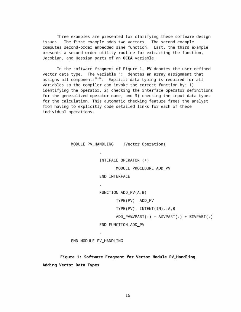
In the software fragment of Figure 1, PV denotes the user-defined vector data type. The variable “:” denotes an array assignment that assigns all components28-30. Explicit data typing is required for all variables so the compiler can invoke the correct function by: 1) identifying the operator, 2) checking the interface operator definitions for the generalized operator name, and 3) checking the input data types for the calculation. This automatic checking feature frees the analyst from having to explicitly code detailed links for each of these individual operations.

MODULE PV_HANDLING !Vector Operations

.

INTEFACE OPERATOR (+)

MODULE PROCEDURE ADD_PV

END INTERFACE

.

FUNCTION ADD_PV(A,B)

TYPE(PV) ADD_PV

TYPE(PV), INTENT(IN)::A,B

ADD_PV%VPART(:) = A%VPART(:) + B%VPART(:)

END FUNCTION ADD_PV

.

END MODULE PV_HANDLING

Figure 1: Software Fragment for Vector Module PV_Handling

Adding Vector Data Types

At compile time, when the compiler encounters a statement that adds two user-defined vector data types, it automatically builds a link that calls the function routine FUNCTION ADD_PV in Module PV_HANDLING (see Figure 1). The compiler first identifies the addition operator (+), for invoking the correct hidden function call. Next, it identifies the data type(s) involved in the operation. Since user-defined data types are detected (i.e., vector data types), the PV_Handling Module is called to resolve the specific routine to be invoked. In PV_Handling, an interface operator definition is encountered for addition that handles two vector data types (i.e., Module procedure ADD_PV). This information enables the compiler to write a direct link to Function ADD_PV at compile time for evaluating this operation during calculations.

Evaluating a Second-Order OCEA Sine Function

11

An OCEA sine function is a mathematical library object that is included in Module EB_Handling (see Figure 2). A composite function calculation is required for evaluating the sine function (i.e., eb_sin), leading to:

where , , (i.e., vector outer product), and . Very compact models are developed

because user-defined data types for scalar, vector, and tensor objects have been defined. For example, the product DF* A,i,j is evaluated in the Module PT_Handling, where a scalar and tensor product is defined.

FUNCTION EB_SIN( A )TYPE(EB) EB_SINTYPE(EB), INTENT(IN)::ATYPE(PT)::AATREAL(KIND=8)::F,DF,DDFINTEGER::I

!VECTOR OUTTER PRODUCT FOR A*A^` FOR TENSOR OPERATOR DO I=1,NV

AAT%TPART(:,I) = A%V%VPART(:)*A%V%VPART(I) END DO

!FUNCTION AND DERIVATIVE DEFINITIONS F = SIN( A%E ) !FUNCTION

DF = COS( A%E ) !FIRST DERIVATIVEDDF =-SIN( A%E ) !SECOND DERIVATIVE!EMBEDDED FUNCTION DEFINITIONSEB_SIN%E = F;EB_SIN%V = DF*A%V;EB_SIN%T = DDF*AAT + DF*A%TEND FUNCTION EB_SIN

Figure 2: Embedded Sine Function

Extracting Function and (Hidden) Partial Derivative Values

The user gains access to the Function and the hidden partial derivative values by invoking utility routines, such as the partition_vector_data subroutine presented in Figure 3. This utility routine handles vectors consisting of second-order OCEA variables. The input for the utility routine consists of a vector of second-order OCEA variables (i.e.,VAR). The utility routine unpacks the OCEA compound data object by using the SCV operators %E, %V, and %T. The output consists of: 1) the vector part of the data (i.e., VEC:= VAR%E), 2) the Jacobian part of the data (i.e., JAC = VAR%V), and 3) the Hessian part of the data (i.e., HES = VAR%T).

EXAMPLE APPLICATIONS

Three numerical examples are presented. The first problem analyzes a scalar polynomial by several methods. This problem compares the convergence histories for classical and generalized Newton-Raphson methods. The generalized Newton-Raphson method is defined by the multilinear reversion of

12

series model presented in Eq. (6). The second problem solves for a set of Earth-Centered elliposodial coordinates, given Cartesian Coordinates for points on or above the surface of the Earth. A local coordinate system is assumed to rotate with the Earth. A 3x1 vector of nonlinear functions defines the necessary condition for the problem. The solution is obtained by using a vector version of the multilinear reversion of series model presented in Eq. (6). The third problem minimizes the classical nonlinear Rosenbrock Banana function problem. This application combines both generalized gradient search and generalized Newton-Raphson methods.

SUBROUTINE PARTITION_VECTOR_DATA( VAR, VEC, JAC, HES )! THIS PROGRAM ACCEPTS AN EMBEDDED VECTOR-VALUED VARIABLE ! AND RETURNS F(X), JACOBIAN( F(X) ), AND SYMMETRIC HESSIAN( F(X) ). !!..INPUT! VAR VECTOR VARIABLE CONTAINING FUNCTION, 1ST, AND 2ND PARTIALS!..OUTPUT! [VEC, JAC, HES ] = [ F(X), JACOBIAN( F(X) ), HESSIAN ( F(X) ) ]

USE EB_HANDLING !OCEA MODULETYPE(EB), DIMENSION(NF), INTENT(IN):: VARREAL(KIND=8), DIMENSION(NF), INTENT(OUT)::VECREAL(KIND=8), DIMENSION(NF,NF), INTENT(OUT)::JACREAL(KIND=8), DIMENSION(NF,NF,NF), INTENT(OUT)::HESINTEGER::P1, P2

!...FETCH SCALAR PART OF INPUT VECTORVEC = VAR%E

!...FETCH JACOBIAN PART OF INPUT VECTORDO P1 = 1, NV JAC( :, P1 ) = VAR%V%VPART( P1 )

!...FETCH HESSIAN PART OF INPUT VECTOR (Symmetric Part) DO P2 = P1, NV HES( :, P1, P2 ) = VAR%T%TPART( P1, P2 ) END DOEND DORETURNEND SUBROUTINE PARTITION_VECTOR_DATA

Figure 3: Utility Routine for Extracting the Scalar, Jacobian, and Hessian

Scalar Polynomial Example Problem

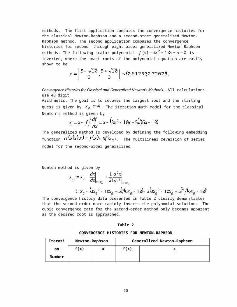
Two scalar polynomial applications are presented, where the goal is to demonstrate accelerated convergence properties for the generalized methods. The first application compares the convergence histories for the classical Newton-Raphson and a second-order generalized Newton-Raphson method. The second application compares the convergence histories for second- through eight-order generalized Newton-Raphson methods. The following scalar polynomial is inverted, where the exact roots of the polynomial equation are easily shown to be

13

.

Convergence Histories for Classical and Generalized Newton’s Methods. All calculations use 40 digit Arithmetic. The goal is to recover the largest root and the starting guess is given by . The iteration math model for the classical Newton’s method is given by

The generalized method is developed by defining the following embedding function . The multilinear reversion of series model for the second-order generalized

Newton method is given by

The convergence history data presented in Table 2 clearly demonstrates that the second-order more rapidly inverts the polynomial solution. The cubic convergence rate for the second-order method only becomes apparent as the desired root is approached.

Table 2

CONVERGENCE HISTORIES FOR NEWTON-RAPHSON

Iteration

Number

Newton-Raphson Generalized Newton-Raphson

f(x) x f(x) x

0 13.00 4.00 13.00 4.00

1 2.59 3.07 1.13 2.89

2 2.83 2.76 9.38x10-3 2.72

3 5.52x10-3 2.72 9.23x10-9 2.72075922

4 2.28x10-6 2.270759 8.85x10-27 2.72075922005612644399963118

Convergence Histories for second- through eighth-order for Generalized Methods. All calculations use 500 digits of numerical precision, because of the rapid convergence of the methods. The polynomial

is inverted using first- through eighth order versions of the generalized Newton-Raphson method, where the convergence rates for are compared in Table 3. The computer symbol

Table 4

RESIDUAL ERROR FOR EXPANSION ORDER VS ITERATION NUMBER.

14

nth

Iteration

F(x) Residual Error VS. Generalized Newton Expansion Order m+

1 2 3 4 5 6 7 8

0 13.00 13.00 13.00 13.00 13.00 13.00 13.00 13.00

1 2.59 1.13 6.1x10-1 3.6x10-1 2.3x10-1 1.5x10-1 1.0x10-1 6.8x10-2

2 2.83 9.4x10-3 1.8x10-4 1.9x10-6 1.0x10-8 2.9x10-11 4.6x10-14 3.9x10-17

3 5.5x10-3 9.4x10-9 2.3x10-18 1.0x10-32 1.1x10-52 4.5x10-79 1.1x10-112 3.0x10-154

4 2.3x10-6 8.9x10-27 6.0x10-74 5.0x10-164 1.9x10-316 * * *

+Numerical precision set to 500 digits for all calculations

*Denotes that the residual error in satisfying f(x) is less than 10-500

manipulation program MACSYMA® has been used to generate a variable-order generalized Newton-Raphson solution algorithm for the calculation. It is surprising to note that all of the first corrections are approximately equal. Only at the second iteration do the residual errors for the roots of f(x) begin to separate in magnitude as a function of the expansion order. The accelerated convergence properties of the higher-order versions of order generalized Newton-Raphson are readily evident. The fourth iteration produces solutions with greater than 500 digits of precision for the sixth-, seventh- and eighth-order versions of the expansion.

Conversion From Geocentric To Geodetic Coordinates

Iterative algorithms are extensively used in computational geodesy for solving the conversion from geocentric to geodetic coordinates17-23. Earth-centered geodetic coordinates are recovered from an earth-fixed rotating coordinate frame. Geodetic coordinates are used in many practical applications for referencing position relative to the Earth. Transformations of this type appear in mapping problems and GPS tracking applications. Spherical coordinates are inconvenient for two reasons. First, the geocentric latitude is not exactly the same as the geographic latitude used in navigation. This is because the Earth is actually an oblate spheroid, slightly flattened at the poles. Second, radius from the Earth's center is an unwieldy coordinate. In the geodetic coordinate system, the coordinates are altitude, longitude, and latitude. Geodetic latitude and longitude are the same latitude and longitude used in navigation and on maps. Geodetic and geocentric longitudes are the same. The position vector for the earth centered earth-fixed XYZ coordinates is given by: where , r = x,y,z denote earth fixed unit vectors for the earth-fixed XYZ coordinates. The desired ellipsodial geodetic coordinates are , which represent the geodetic latitude, longitude and the height above the surface of the Earth. The geodetic and Cartesian coordinates are defined by the following functional relationship between the variables , , , and

, where x,y,z denote specified earth centered Cartesian coordinates, denotes the

radius of curvature in the prime vertical plane, a = 6378.160km denotes the major earth axis (ellipsoid equatorial radius), denotes the semi-minor earth axis (ellipsoid polar radius), f = (a-b)/a

denotes the flattening factor, and =0.00669454185 denotes the eccentricity squared. The equations are highly nonlinear and coupled.

15

Starting solutions for the generalized Newton-Raphson method are obtained by expanding the transformation equations above about , leading to the vector-valued starting guess (assuming that z is not approximately 0)

From the multilinear reversion of series solution presented in Eq. (6), a fourth-order solution for the elliptical coordinate inversion problem is defined by

The partial derivative models for the rates in Eq. (9) are too complicated to present here. The results of a single iteration of the algorithm are presented in Table 4, where the accuracy of each order of the approximation is evaluated. The maximum initial error is approximately 104m. At second-order in the expansion, the residual errors have been reduced to ~6mm (six orders of magnitude reduction). The third and fourth order terms of the series produce solution accuracy’s far exceeding the useful precision limits of real-world applications. Repeating the process using the first iteration solution as the starting guess increases the solution accuracy to beyond machine double precision.

Table 4

ELLIPTICAL COORDINATE INVERSION ERROR VS. SERIES ORDER

Correction Terms Position Vector Component Errors (meters)

Reversion of Series

Order

DX DY DZ

0 4.31x103 4.89x103 -23.2x103

1 -2.77x101 -3.14x101 -3.25x10-2

2 6.81x10-2 7.22x10-2 5.93x10-3

3 -1.28x10-4 -1.45x10-4 -3.78x10-5

4 9.94x10-8 1.13x10-7 1.66x10-7

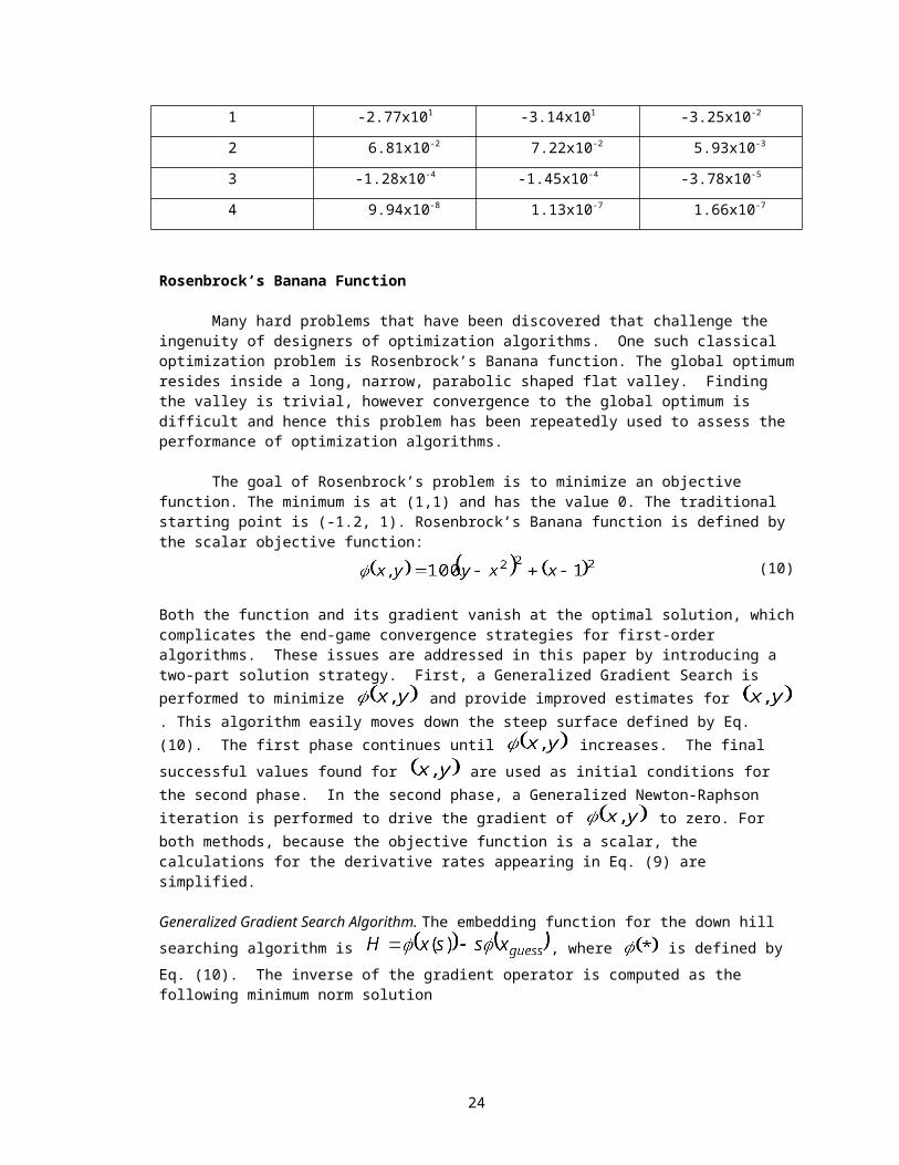
Rosenbrock’s Banana Function

Many hard problems that have been discovered that challenge the ingenuity of designers of optimization algorithms. One such classical optimization problem is Rosenbrock’s Banana function. The global optimum resides inside a long, narrow, parabolic shaped flat valley. Finding the valley is trivial, however convergence to the global optimum is difficult and hence this problem has been repeatedly used to assess the performance of optimization algorithms.

16

The goal of Rosenbrock’s problem is to minimize an objective function. The minimum is at (1,1) and has the value 0. The traditional starting point is (-1.2, 1). Rosenbrock’s Banana function is defined by the scalar objective function:

(10)

Both the function and its gradient vanish at the optimal solution, which complicates the end-game convergence strategies for first-order algorithms. These issues are addressed in this paper by introducing a two-part solution strategy. First, a Generalized Gradient Search is performed to minimize and provide improved estimates for . This algorithm easily moves down the steep surface defined by Eq. (10). The first phase continues until increases. The final successful values found for are used as initial conditions for the second phase. In the second phase, a Generalized Newton-Raphson iteration is performed to drive the gradient of to zero. For both methods, because the objective function is a scalar, the calculations for the derivative rates appearing in Eq. (9) are simplified.

Generalized Gradient Search Algorithm. The embedding function for the down hill searching algorithm is , where is defined by Eq. (10). The inverse of the gradient operator is

computed as the following minimum norm solution

(11)

This equation is only useful as long as the gradient does not vanish. From Eqs. (6) and (9) one obtains the following simplified rate equations for the multilinear reversion of series coefficients

(12)

where and

This equation is cycled until increases, by replacing .Generalized Newton-Raphson Algorithm. After completing the down hill search phase of the optimization problem, a Generalized Newton-Raphson algorithm is started to complete the solution. The goal is to drive the gradient values of the objective function to zero. The embedding function for the newton-like algorithm is , where is defined by Eq. (10). . From Eq. (9) one obtains the following simplified rate equations for the multilinear reversion of series coefficients

17

Only three derivative rates are retained, because OCEA currently only supports first through fourth order gradient calculations. From the multilinear reversion of series expansion of Eq. (6), the generalized Newton-Raphson algorithm is given by

(13)

This equation is cycled until the , where is a prescribed convergence tolerance.Optimizing Rosenbrock’s Banana Function. Two example problems are considered for solving Rosenbrock’s Banana problem. The first example is presented in Figure 4a, where the traditional starting values for (x,y) = (-1.2, 1.0) are used. These initial conditions force the algorithm to handle the local region of high curvature presented in Figure 4a. Six iterations are required for recovering the optimal values with double precision accuracy for both the function and its gradient values (function value ~ 10-39

and the gradient value ~ (10-20,10-20) ). This remarkably rapid convergence should be compared to reported results for the currently best optimization algorithms that typically take hundreds of iterations to achieve only three to four digits of precision. The numerical values encountered during the iteration process are summarized in the Table 5. Unlike traditional optimization algorithms, the OCEA-enabled generalized gradient search and Newton-Raphson algorithms demonstrate robust and rapid end-game performance as the solution approaches the optimal values.

Table 6CONVERGENCE HISTORY FOR ROSENBROCK FUNCTION

Function At Each Correction Order

Iteration Method Starting

Function

1st 2nd 3rd 4th

1 GGS* 24.2 7.63 5.20 4.42 4.16

2 GGS Failed 4.16 85.9

3 GNR* 85.9 2.33 2.36 2.38

4 GNR 2.38 409 10.8 0.153

5 GNR 0.153 4.3x10-7 3.3x10-7 2.6x10-7

6 GNR 2.6x10-7 6.9x10-12 1.0x10-21 1.0x10-39

GGS* Denotes Generalized Gradient Search

GNR* Denotes Generalized Newton-Raphson

The second example considers a more difficult starting position the algorithm. The assumed initial values are (x, y) = (-3.5, -3.5), which is located on the opposite side of the local hill where the optimal solution lies. As is the first case, the algorithm converges very rapidly, requiring only five iterations for achieving double precision solution accuracy for both the function and its gradient.

18

19

20

Figure 4a Convergence History for Rosenbrock’s Function

21

CONCLUSIONS CONCLUSIONS

22

Figure 4b Convergence History for Challenging Starting Conditions for Rosenbrock’s Function

New and powerful root-solving and optimization algorithms have been presented and demonstrated to handle non-trivial applications with relative ease. A multilinear reversion of series algorithm has been presented that replaces a very difficult iteration algorithm with a closed-form solution algorithm. The reversion of series algorithm is shown to be a direct generalization of the classical Newton’s method and its various accelerated convergence variations. New algorithms provide analytic high order approximations for scalars, matrix and tensor applications. High order partial derivative models are handled by introducing automated differentiation techniques. The OCEA algorithm is presented for managing and building the automated differentiation tools. OCEA completely frees the analyst from having to model, code, and validate complicated partial derivative models. The partial derivative models (i.e., first through fourth order) are exact and accurate to the working precision of the machine. The proposed methods are expected to have broad potential for impacting the theory and design of advanced mathematical programming tools for knowledge discovery applications.

Future developments must address computational issues for improving the efficiency of the prototype tools presented herein. Key remaining issues include: variable order tools, discontinuous derivatives, event handling for special limiting cases, symmetry, sparse structure, and parallel implementation.

23

REFERENCES

1. Newton, Methodus fluxionum et serierum infinitarum, (1664-1671).2. J. Raphson, Analysis Aequationum universalis, London, (1690).3. A. S. Householder, The Numerical Treatment of a Single Nonlinear Equation, McGraw-Hill, New

York, (1970). 4. J. D. Turner, “Object Oriented Coordinate Embedding Algorithm For Automatically Generating the

Jacobian and Hessian Partial Derivatives of Nonlinear Vector Function,” Invention Disclosure, University of Iowa, May 2002.

5. J. D. Turner, “The Application of Clifford Algebras for Computing the Sensitivity Partial Derivatives of Linked Mechanical Systems,” Invited Paper presented to Mini-Symposium: Nonlinear Dynamics and Control, USNCTAM14: Fourteenth U.S. National Congress Of Theoretical and Applied Mechanics, Blacksburg, Virginia USA, June 23-28, 2002.

6. J. D. Turner, “Automated Generation of High-Order Partial Derivative Models,” To Appear, AIAA Journal, August 2002.

7. L. R. Nyhoff, Introduction to FORTRAN 90 for Engineers and Scientists, Prentice Hall, ISBN 0135052157, 1996.

8. W. H. Press, and W.T. Vetterling, Numerical Recipes in FORTRAN 90, Vol.2, Cambridge, ISBN 0521574390, 1996.

9. L. P. Meissner, FORTRAN 90, PWS Publishers, ISBN 0534933726, 95.10. J. L. Junkins, and J. D. Turner, Optimal Spacecraft Rotational Maneuvers: Studies in Astronautics,

Vol. 3, Elsevier Science Publishers, Amsterdam, The Netherlands, 1986. 11. A. Griewank, “On Automatic Differentiation” in Mathematical Programming: Recent Developments

and Applications, edited by M. Iri and K. Tanabe, Kluwer Academic Publishers, Amsterdam, 1989, pp. 83-108.

12. C. Bischof, A. Carle, G. Corliss, A. Griewank, and P. Hovland, “ADIFOR: Generating Derivative Codes from Fortran Programs,” Scientific Programming, V.1, 1992, pp.1-29.

13. C. Bishchof, A. Carle, P. Khademi, A. Mauer, and P. Hovland. “ADIFOR 2.0 User’s Guide (Revision CO, “ Technical Report ANL/MCS-TM-192, Mathematics and computer Science Division, Argonne National Laboratory, Argonne, IL., 1995.

14. P. Eberhard and C. Bischof. “Automatic Differentiation of Numerical Integration Algorithms,” Technical Report ANL/MCS-P621-1196, Mathematics and Computer Science Division, Argonne National Laboratory, Argonne, IL, 1996.

15. http://numbers.computation.free.fr/Constants/Algorithms/newton.html 16. Macsyma, Symbolic/numeric/graphical mathematics software: Mathematics and System Reference

Manual, 16th edition, Macsyma, Inc. 1996.17. Astronomical Almanac for the Year, USNO and RGO, Washington and London, p. K11, 1987.18. K. M. BORKOWSKI, Transformation of Geocentric to Geodetic Coordinates without Approximations,

Astrophys. Space Sci., 139, pp. 1–4, 1987.19. D. R. HEDGLEY, “An Exact Transformation from Geocentric to Geodetic Coordinates for Nonzero

Altitudes,” NASA Techn. Rep. R–458, 1976.20. S. A. T. LONG, “General Altitude Transformation between Geocentric and Geodetic Coordinates,”

Celestial Mech., 12, 225–230, 1975.21. J. MORRISON and S. PINES, “The Reduction from Geocentric to Geodetic Coordinates,” Astron. J.,

66, 15–16, 1961.22. M. K. PAUL, “A Note on Computation of Geodetic Coordinates from Geocentric (Cartesian)

Coordinates,” Bull. Géod., Nouv. Ser., No 108, 1973, pp.135–139.23. M . PICK, “Closed Formulae for Transformation of the Cartesian Coordinate System into a System of

Geodetic Coordinates,” Studia geoph. et geod., Vol. 29, 1985, pp. 112–119.24. Richard H.Battin, An Introduction to the Mathematics and Methods of Astrodynamics, AIAA

Education Series, 1987.

24

25