intelligent multi-resolution modeling: application to...

Intelligent Multi-Resolut ion Modelling: Application to Synthetic Jet Actuation and

Flow Control Puneet Singla: John L. Junkinst Othon ~ediniotist

Texas A & M University, 3141-TAMU, College Station, TX 77843-3141 Kamesh Subbaraos

Unzversity of Texas, Arlington, B o x 1901 8, 21 1 Woolf Hall, Arlington, TX 76019-0018

A novel "directed graph" based algorithm is presented that facilitates intelligent learning and adaptation of the parameters appearing in a Radial Basis Function Network (RBFN) description of input output behavior of nonlinear dynamical systems. Several alternate for- mulations, that enforce minimal parameterization of the RBFN parameters are presented. An Extended Kalman Filter algorithm is incorporated to estimate the model parameters using multiple windows of the batch input-output data. The eficacy of the learning algorithms are evaluated on judiciously constructed test data before implementing them on real aerodynamic lip and pitching moment data obtained from experiments on a Synthetic Jet Actuation based Smart Wing.

Introduction There is a significant thrust in the aerospace indus-

try to develop advanced nano technologies that would enable one to develop adaptive, intelligent, shape con- trollable micro and macro structures, for advanced aircraft and space systems. These designs involve pre- cise control of the shape of the structures with micro and nano level manipulations (actuation). The issue at hand is to derive comprehensive mathematical models that capture the input output behavior of these structures so that one can derive automatic control laws that can command desired shape and behavior changes in the structures. The development of the models using first principles, from classical mechanics fails at micro and nano scales and quantum mechanics applies only at scales less than pico-level. Thus, there is a lack of a unified modelling approach to derive macro models from those at the nano and micro scales. While the conventional modelling approaches evolve to han- dle these problems, one can pursue non parametric,

"Graduate Assistant Research, Student Member AIAA, De- partment of Aerospace Engineering, Texas A&M University, College Station, TX-77843, puneetOtamu.edu.

t~ i s t in~uished Professor, George Eppright Chair, AIAA Fel- low, Department of Aerospace Engineering, Texas A&M Uni- versity, College Station, TX-77843, junkinsOtamu.edu.

t~ssoc iate Professor, AIAA Associate Fellow, Department of Aerospace Engineering, Texas A&M University, College Station, TX-77843, [email protected].

S~ssistant Professor, AIAA Member, Department of Me- chanical and Aerospace Engineering, University of Texas, Ar- lington, TX, subbarmOmae.uta.edu.

Copyright @ 2004 by the American Institute of Aeronautics and Astronautics, Inc. No copyright is asserted in the United States under Title 17, US. Code. The US. Government has a royalty- free license to exercise all rights under the copyright claimed herein for Governmental Purposes. All other rights are reserved by the copyright owner.

multi-resolution, adaptive input/output modelling a p proaches to capture macro static and dynamic models directly from experiments. The purpose of this paper is to present an algorithm to learn a non-parametric mathematical model based upon radial basis functions that in essence aggregates information from large number of sensor measurements distributed over the structure. This aggregated information can be used to distribute actuation at specific points of the structure to achieve a desired shape. We will show the application of this algorithm to learn the mapping between the synthetic jet actuation parameters (frequency, direction, etc. for each actuator) and the resulting aerodynamic lift, drag, and moment.

Synthetic jet actuators (SJA) are devices used for active flow control that enable enhanced performance of conventional aerodynamic surfaces at high angles of attack and in many cases could lead to full replacement of hinged control surfaces thereby achieving perfect hingeless control. This active flow control is achieved by embedding sensors and actuators at nano and micro scales on an aerodynamic structure as shown in figure 1. The desired force and moment profile is achieved by impinging a jet of air using these actuators and thereby creating a desired pressure distribution over the structure. The distinguishing feature of synthetic jet actuation problem is that the relationship between input and output variables is not well known and is nonlinear in nature. Further, un-steady flow effects make it impossible to capture the physics fully from static experiments. The central difficulty in learning input/output mapping lies in choosing appropriate basis functions. While the brute force approach of using infinitely many basis functions is a theoretical possibil- ity, it is intractable in a practical application because

1 OF 13

AMERICAN INSTITUTE OF AERONAUTICS AND ASTRONAUTICS PAPER 2004-0774

42nd AIAA Aerospace Sciences Meeting and Exhibit5 - 8 January 2004, Reno, Nevada

AIAA 2004-774

Copyright © 2004 by Puneet Singla, Kamesh Subbarao, John L Junkins, Othon Redionitis. Published by the American Institute of Aeronautics and Astronautics, Inc., with permission.

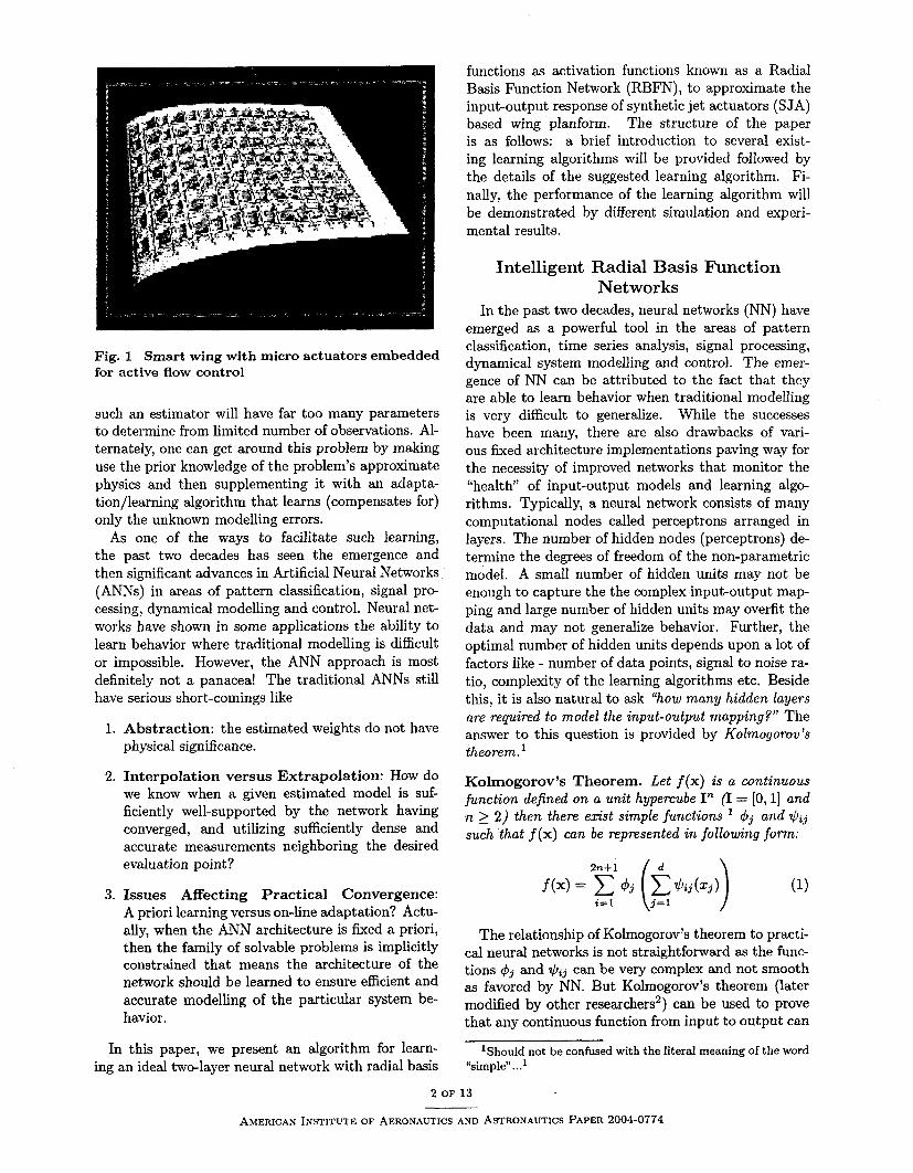
Fig. 1 Smart wing with micro actuators embedded for active flow control

such an estimator will have far too many parameters to determine from limited number of observations. Al- ternately, one can get around this problem by making use the prior knowledge of the problem's approximate physics and then supplementing it with an adaptation/learning algorithm that learns (compensates for) only the unknown modelling errors.

As one of the ways to facilitate such learning, the past two decades has seen the emergence and then significant advances in Artificial Neural Networks (ANNs) in areas of pattern classification, signal processing, dynamical modelling and control. Neural networks have shown in some applications the ability to learn behavior where traditional modelling is difficult or impossible. However, the ANN approach is most definitely not a panacea! The traditional ANNs still have serious short-comings like

Abstraction: the estimated weights do not have physical significance.

Interpolation versus Extrapolation: How do we know when a given estimated model is sufficiently well-supported by the network having converged, and utilizing sufficiently dense and accurate measurements neighboring the desired evaluation point?

Issues Affecting Practical Convergence: A priori learning versus on-line adaptation? Actu- ally, when the ANN architecture is fixed a priori, then the family of solvable problems is implicitly constrained that means the architecture of the network should be learned to ensure efficient and accurate modelling of the particular system behavior.

In this paper, we present an algorithm for learning an ideal two-layer neural network with radial basis

functions as activation functions known as a Radial Basis Function Network (RBFN), to approximate the input-output response of synthetic jet actuators (SJA) based wing planform. The structure of the paper is as follows: a brief introduction to several existing learning algorithms will be provided followed by the details of the suggested learning algorithm. Fi- nally, the performance of the learning algorithm will be demonstrated by different simulation and experimental results.

Intelligent Radial Basis Function Networks

In the past two decades, neural networks (NN) have emerged as a powerful tool in the areas of pattern classification, time series analysis, signal processing, dynamical system modelling and control. The emergence of NN can be attributed to the fact that they are able to learn behavior when traditional modelling is very difficult to generalize. While the successes have been many, there are also drawbacks of various fixed architecture implementations paving way for the necessity of improved networks that monitor the "health" of input-output models and learning algorithms. Typically, a neural network consists of many computational nodes called perceptrons arranged in layers. The number of hidden nodes (perceptrons) determine the degrees of freedom of the non-parametric model. A small number of hidden units may not be enough to capture the the complex input-output m a p ping and large number of hidden units may overfit the data and may not generalize behavior. Further, the optimal number of hidden units depends upon a lot of factors like - number of data points, signal to noise ra- tio, complexity of the learning algorithms etc. Beside this, it is also natural to ask "how many hidden layers are required to model the input-output mapping?" The answer to this question is provided by Kolmogorov's theorem.'

Kolmogorov's Theorem. Let f(x) i s a continuous function defined on a unit hypercube I n (l = [O, 11 and n 2 2 ) then there exist simple functions q5j and qij such that f (x) can be represented in following form:

The relationship of Kolmogorov's theorem to practical neural networks is not straightfornard as the functions dj and qij can be very complex and not smooth as favored by NN. But Kolmogorov's theorem (later modified by other researchers2) can be used to prove that any continuous function from input to output can --

'Should not be confused with the literal meaning of the word "simplen ...I


be approximated by a two layer neural n e t ~ o r k . ~ A more intuitive proof can be constructed by the fact that any continuous function can be approximated by an infinite sum of harmonic functions. Another anal- ogy is the reference to bump or delta functions i.e. a large number of delta functions at different input locations can be put together to give the desired f ~ n c t i o n . ~ Such localized bumps might be implemented in a number of ways for instance by Radial basis functions.

Radial basis function based neural networks are two- layer neural networks with node characteristics described by radial basis functions. Originally, they were developed for performing exact multivariate interpolation and the technique consists of approximating a non-linear function as the weighted sum of a set of radial basis functions.

h

f ( 4 = C w , M x - pill) = wT@(llx - ~11) (2) i=l

where, x E Rn is an input vector, Q, is a vector of h radial basis functions with pi as the center of ith radial basis function and w is a vector of linear weights or amplitudes. The two layers in RBFN per- form two different tasks. The hidden layer with radial basis function performs a non-linear transformation of the input space into a high dimensional hidden space whereas the outer layer of weights performs the linear regression of this hidden space to achieve the desired value. The linear transformation followed by a nonlinear one is summarized in Cover's theorem3 as follows,

Cover's Theorem. A complex pattern classification problem or input/output problem cast in a high- dimensional space is more likely to be approximately linearly separable than in a low-dimensional space.

According to Cover and Kolmogorov's theorems Multilayered Neural networks (MLNN) and RBFN can serve as "Universal Approximators". While MLNN performs a global and distributed approximation at the expense of high parametric dimensionality,RBFN gives a global approximation but with locally dominant basis functions.

The main feature of radial basis functions (RBF) is that they are locally dominant and their response decreases (or increases) monotonically with distance from their center. This is ideally suited to modelling input-output behavior that shows strong local influ- ence as with the synthetic jet actuation experiment. Some examples of RBF are:4

Thin-plate-spline function: 4( r ) = r2 log r

Multiquadric function: +(r) = (r2 + a2)'I2

Inverse Multiquadric function: 4(r) = (r2 + a2)-lI2

Gaussian function: +(r) = exp(-r2/a2)

where r represents the distance between a center and the data points, usually taken to be Euclidean distance. a is a real variable; for Gaussian functions it is a measure of the spread of the function. Among the above mentioned RBF, the Gaussian function is most widely used because its response can be confined to local dominance without altering the global approximation. Beside this, the shape of the Gaus- sian functions can also be adjusted appropriately by altering the parameters appearing in its description. To summarize in general, the parameters needed to construct an RBFN can be enumerated as follows:

1. Number of RBF, h

2. The center of RBF, p,

3. The spread of RBF ( ai in case of Gaussian function)

4. The linear weights between hidden layer and the output layer, wi

An adaptable, intelligent network would seek to update/learn some or all of the above mentioned parameters. Most importantly, the different learning parameters of RBFN live in the space of the in- puts thereby enabling a physical interpretation of the parameters. This adaptation of the architecture of RBFN leads to a new class of approximators suitable for multi-resolution approximation applications. Con- ventionally (historically), the following form for the n-dimensional Gaussian functions is adopted,

where, PC' = diag(ak - + . a:,). To learn the parameters mentioned above, different learning algorithms have been developed in the literature ,5.6

Poggio and Girosi7 introduced the traditional regu- larization technique to learn these parameters. Their RBFN has two layers with fixed number of hidden units (nodes) and center of hidden units chosen as a subset of the input samples. Algorithms such as forward selection can be used to find that subset. The linear weights connecting hidden layer to output layer can be found by Gradient Descent methods. The main disadvantage of this particular approach is the high computational cost involved. Besides this, a judicious choice of initial guess for weights is required as the algorithm can get stuck a t local minima.

Moody and Darkens introduced a low computation cost method which involves the concept of locally tuned neurons. Their algorithm takes the advantages of local methods conventionally used for density estimation, interpolation and approximation. Here too, the number of hidden units are chosen a priori. They used a standard k-means clustering algorithm to estimate the centers of the RBF and computed the

3 OF 13


width values using various N nearest-neighbor heuris- tics. While k-means is suitable for pattern classification, it may not guarantee good results for function approximation because two samples close to each other in input space do not necessarily have similar

In 1991, Cheng proposed an algorithm, known as Orthogonal Least Squares (OLS) which makes use of Gram-Schmidt type orthogonal projection to select the best centers at a time. Starting from a large pool of candidate centers, OLS selects the predetermined number of centers that result in the largest reduction of error at output. Since it is not necessary that predetermined number of hidden units will always give us good approximation, Lee and Killo proposed a Hier- archically Self-organizing learning algorithm which is capable of automatically recruiting new hidden units whenever necessary.

Also in 1991, Plattll proposed a sequential learning RBFN known as Resource Allocating Network (RAN). The network proposed by Platt learns by allocating a new hidden unit or adjusting the parameters of existing hidden units for each input data. If the network performs well on a presented pattern, then the network parameters are updated using standard least mean squares gradient descent otherwise a new hidden unit is added to correct the response of the earlier network. A variation of this algorithm1' using extended Kalman filter13 for parameter adaptation is proposed by N. Sundararajan known as MRAN (Modified Re- source Allocating Network). The advantages of RAN over any other learning algorithms can be summarized as follows.

It is inherently sequential in nature and therefore can be used recursively in real-time to update the estimated model

The network architecture itself is adapted in con- trast to adjusting weights in a fixed architecture network.

The adaptive architecture feature and the inher- ent recursive structure of the learning algorithm makes this approach ideal for multi-resolution modelling.lO* l 2 7 l4 While the methodology is very effective, it suffers from the drawback of potential explosion in the number of basis functions utilized to approximate the functional behavior. The reason for this stems from the fact that almost always, the basis functions are chosen to be circular. In some cases, the widths of the basis functions are chosen to be different. While this aids in improving the resolution, it does not significantly help in the reduction of the number of basis functions required. To overcome this problem, a pruning strategy is used posteriori4 but the convergence of network size is not guaranteed.

In the next section, we will propose an "Intelligent" scheme that sequentially learns the orientation of the

data set with a fresh batch of data (can be in real time) and changes the orientation of the basis function, along with tuning of the centers and widths to enlarge the scope of a single basis function to approximate as much of the data possible. We see that this helps in reducing the overall number of basis functions and improving the function approximation accuracy. The orientation of the radial basis function can be modelled through a rotation parameter which for the two and three dimensional cases can be shown to the tangent of the half angle of the principal rotation vector.

Direction Dependent Approach In this section, we present a novel learning algo-

rithm for RBFN learning that is motivated through developments in rigid body rotational kinematics. The development is novel because of the application of the rotation ideas to the function approximation problem. We try to move as well as rotate the Gaussian basis function to expand coverage, thereby reducing the t c ~ tal number of basis functions required for learning.

We propose adoption of the following n-dimensional Gaussian function:

Where, P is n x n fully populated symmetric positive definite matrix instead of diagonal one as in the case of conventional Gaussian function given by equation (3). Now using spectral decomposition P-l can be written as:

pi1 = ~ ( q i ) ~ ( a , ) ~ ~ ( q ~ ) (5)

Where S is a diagonal matrix containing the eigen- values, ai, of covariance matrix Pi which dictates the spread of Gaussian function Qi. C(qi) is a n x n orthogonal rotation matrix. Though C(qi) is a n x n square matrix, we require only 9 minimal parameters to describe it due to the orthogonality constraint. To enforce this constraint, we parameterize the matrix C(q,) using the rotation parameter through the following result in matrix theory that is widely used in attitude kinematics namely, the Cayley Transforma- tion.15

Cayley Transformation. If C E RnXn is an orthogonal m a t e and Q E Rnxn is an skew-symmetric matrix then the following transformations hold:

1. Forward Tmnsfomations

2. Inverse Transformations

(a) Q = (I - C) (I + c)-'

(b) Q = (I+ C)-l(I - C )

As any arbitrary proper orthogonal matrix can be substituted into the above written transformations, Cayley Transformations can be used to parameterize the entire O(n) group by skew symmetric matrices. The forward transformation is always well behaved however the inverse transformation encounter difficulty only near 180' rotation. Thus as per the Cayley transformation, we can parameterize the orthogonal matrix C(qi) in equation (5) as:

where, qi is a vector of distinct elements of skew symmetric matrix Q i.e. Q = - Q ~ . In addition to the parameters mentioned in last section, we now have to learn the additional parameters characterizing the orthogonal rotation matrix making total ! n f 2 ) z ( n + 1 ) parameters per Gaussian function for n input single output system.

1. n parameters for center of the Gaussian function i.e. p.

2. n parameters for spread of Gaussian function i.e. u.

n(n-1) 3. 7 parameters for rotation of Gaussian function.

4. Weight wi corresponding to one output.

We shall develop learning algorithms for this extended parameter set. To our knowledge, this parameterization is unique and preliminary studies indicate a significant reduction in the number of basis functions required to accurately model functional behavior of the actual input output data.

The main feature of the proposed learning algorithms is the judicious choice for the location of the RBFs via a Directed Connectivity Graph approach which allows a priori adaptive sizing of the network for off-line learning and zeroth order network pruning. Be- side this, Direction Dependent scaling and rotation of basis functions is provided for maximal trend sensing with minimal parameter representations and adaptation of the network parameters is done to account for on-line tuning.

Directed Connectivity Graph The first step towards obtaining a zeroth order off-

line model is the judicious choice of a set of basis functions and their locations, followed by proper ini- tialization of the parameters. This exercise is the focus of this section.

To find the local extremum points of a given surface data, we divide the input space into several subspaces with the help of a priori prescribed hypercubes and find the relative maximum and minimum in each s u b space. Now the set of extremum points of the surface data will be the subset of these relative maxima and

minima for a particular size of the hypercube. Fur- ther, to choose centers out of these relative maxima and minima we construct directed graphs M and N of all the relative maxima sorted in descending order and all the relative minima sorted in ascending order respectively. We then choose the first points in M and N as candidates for Gaussian function centers with the function value as the corresponding starting weight of the Gaussian functions. The initial value of the covariance matrix P is found by applying a local mask around the chosen center. Now using all the input data, we adapt the parameters of the chosen Gaussian functions sequentially using the extended Kalman fil- terl3?l6 and check the error residuals for estimation error. If the error residuals do not satisfy a prede- fined bound, we choose the next points in the directed graphs M and N as additional Gaussian RBF and repeat the whole process.

Notice, that the above choice of the Gaussian functions and the location of the centers is set around the fact that Gaussian functions are log-concave and this construction facilitates the evaluation of the extremal points.

Definition 1. A function f : V c Rn -, R C R is concave if (-f) i s a convex function i.e. if V i s a convex set and V X, y E V and &(0, I) , we have

In other words f (x) is a concave function if a line segment joining (x, f (x)) and (y, f (y)) lies below the graph of f (x). Further if f is a differentiable function then it can be shown that equation (7) is equivalent to following condition:

The above-mentioned inequality leads to the following important property of a concave function.17

Lemma. Let a function f : V C Wn t R C W i s concave and differentiable then a point xcV i s a global maximum iff 2 1, = 0.

Proof. The proof can be found in Ref. 17 0

These results along with the following definition and properties of the log-concave function,17 provides a theoretical basis for the specific choice of the RBF in this paper.

Definition 2. A function f : V W n + R C R i s log-concave if f (x) > 0 for all XED and log f i s concave.

Thus, to choose the location of the RBF centers, we make use of the fact that a Gaussian function is log- concave in nature and the response of the logarithm of


the Gaussian function is maximum at its center making the center of this function the extremum point i.e. -I,=, = 0 as per the above-mentioned lemma. Further, since log is a monotonically increasing function the center of the Gaussian function is also an extremum point of the Gaussian function. Therefore, all the extremum points of the given surface data should be the first choice for centers of Gaussian function with spread determined to first order by the covariance of the data confined in local mask around particular extremum point.

Though this whole process of finding the centers and evaluating the local covariance followed by the function evaluation with adaptation and learning seems computationally extensive it helps in reducing the total number of Gaussian functions and keeping the "curse of dimensionality" in check. Further, the rotation parameter of Gaussian function enables us to approximate the function with a greater accuracy. Since we use the Kalman filter to learn the parameters of the RBF network, the selection of centers can be made off-line with some experimental data and the same algorithm can be invoked online to adapt the parameters of off-line network. Any new Gaussian centers can be added to the existing network depending upon the statistics information of approximation errors. Ad- ditional localization and reduction in computational burden can be achieved by exploiting the local dominance, near a given point, on only a small subset of RBFN parameters. Further information on the online version of the algorithm is presented in Ref.18.

Extended Kalman Filter

Kalman filtering is a relatively recent (1960) development in the field of estimation.l31" However, it has its roots as far as back in Gauss's work in the 1800's. The only difference between the Kalman filter and the sequential version of the Gaussian least squares is that the Kalman filter uses a dynamical model of plant to propagate the state estimates and corresponding error covariance matrix between two sets of measurements. In parallel with Kalman's linear estimation work (1960), Stanley F. Schmidt proposed the application of the Kalman filter for systems in- volving non-linear dynamic and measurement models and it has been called the "Kalman-Schmidt filter". The extended Kalman filter is based on the assump tion that the estimated state is close to the true state and therefore the error dynamics can be represented as the first order Taylor series expansion of the nonlinear error dynamics. However this assumption can be very fatal for the case of large initial errors or a highly non-linear system. The extended Kalman filter for non-linear systems uses the linearized state space model about the current estimates of the states to generate the current update at a measurement time, but propagates the estimates non-linearly between two

Table 1 Kalman-Schmidt Filter

Measurement Model

I where

with

E ( v k ) = 0

~(zqvz) = Rk6(1-k)

Update

measurement sets. The implementation equations for the extended Kalman filter or LLKalman-Schmidt filter" are given in Table l. The main advantage of the extended Kalman filter is that the nominal trajectory about which linearization takes place can be defined in real time. However, we have to pay the extra computational cost for linearization.

The sensitivity matrix H for the problem at hand is defined as:

P ; = ( I - K k H ) P ;

N where, f (x, p, U, q) = wi@i(Pi, a i , qi) and Q is a N x (n+1)z(n+2) vector given by:

The partial derivatives required for the computation of the sensitivity matrix, H are given as follows:

Notice that, in equation (14) can be computed


by substituting for C from equation (6):

Making use of the fact that (I - &)-I (I - Q) = I, we get

(16) substitution of equation (16) in equation (15) gives:

1 dQk + Qk) + (I - Qk)- - &kl

(17)

Now equations (11)-(14) constitute the sensitivity matrix H for the Extended Kalman Filter. We mention that although equation (5) provides a minimal parametrization of the covariance matrix P, it is highly nonlinear in nature and causes problems in the convergence of the Kalman filter in certain cases. To alleviate this potential difficulty and improve computational speed, we present an alternate representation the covariance matrix P known as Additive Decompo- sition.

Additive Decomposition of Covariance Matrix P In this approach, we introduce the following param-

eterization of positive definite matrices:

Additive Decomposition. Let P be a symmetric positive definite n x n matrix then P-' i s also symmetric and positive definite and can be written as a sum of a diagonal matrix and a symmetric matrix:

where ei i s a n x 1 vector with only ith element equal to one and rest of them zeros and rk i s a diagonal matrix given by:

1

subject to following constraints:

It is worthwhile to mention that qkij signifies the stretching and rotation of the Gaussian function. If

qkij = 0 then we will obtain the circular Gaussian function.

Using the additive decomposition for the Pi matrix in equation (4) the different partial derivatives required for synthesizing the sensitivity matrix H can be computed by defining the following parameter vector O

@ = ( wl pi 0 1 q l " ' wN pjv ON q N ) (24)

The different partial's are then given as follows:

'a f - - dwk

- d'k

Thus, equations (25)-(28) constitute the sensitivity matrix H. It is to be mentioned that even though the synthesis of the sensitivity matrix is greatly simplified, one needs to check the constraint satisfaction defined in equations (20)-(23) at every update. In case these constraints are violated, we invoke the parameter projection method to project the parameters back to the sets they belong to, thereby ensuring that the covariance matrix remains symmetric and positive definite at all times.

The various steps for the Directed Connectivity Graph Learning Algorithm are summarized as follows:

1. Find the interior extremum points of the given surface-data.

2. Divide the Input space into several subspaces with the help of equally spaced 1 - D rays so that extremum points do not fall on the boundary of any subregion.

3. Find the relative maximum and minimum in each region.

4. Make a directed graph of all the maximum points sorted in descending order and call it M.

5. Make a directed graph of all the minimum points sorted in ascending order and call it N.

6. Choose first point in M and N as a candidate for Gaussian center and function values as the weight of those Gaussian functions.

7. For these points find the associated covariance matrix (P) with the help of local mask.

8. Initialize qij = Pi,. and a = 0.


Learn w, p, u, qi j using extended Kalman filter (Table 1) with the help of whole data.

Make sure that new estimated parameter vector satisfy the constraints given by equations (20-23)

Check the estimation error residuals. If they do not satisfy the required accuracy limit then choose second point in set M and N as Gaussian center and follow from step 7.

Numerical Simulations and Results This algorithm was tested on a variety of test func-

tions and experimental data obtained by wind tunnel testing of synthetic jet actuation wing. In this section, we will present some results from the studies, importantly a test case for function Approximation and a dynamical System identification from wind tunnel testing of synthetic jet actuation wing.

Function Approximation

The test case for the function approximation is motivated by the following analytic surface function.lg

A random sampling of the interval 10 - 10,0 - 101 for X I and x2 is used to obtain 60 samples of each. Fig- ures 2(a) and 2(b) show the true surface and contour plots of the training set data points respectively. Ac- cording to our experience this particular function has many important features such as sharp ridge line that is very difficult to learn with many existing function approximation algorithms with reasonable number of nodes. The failure of these many RBFN learning algorithms can be attributed to the inability of the circular Gaussian function to approximate a ridge kind of surface globally.

To approximate the function given in equation (29), we divide the whole input region into a total of 16 square regions (4 in each direction). Then according to the procedure listed in the previous section, we generate a directed connectivity graph of the local maxima and minima in each subregion that finally add up to 32 radial basis functions to have approximation errors less than 5%. Figures 2(c) and 2(d) show the estimated surface and contour plots respectively. From these figures, it is clear that we are able to learn the analytical function given in equation (29) very well. Figures 2(e) and 2(f) show the error surface and error contour plots for the RBFN approximated function. From figure 2(e), it is clear that approximation errors are less than 5% whereas from figure 2(f) it is clear

that even though we approximate the ramp surface very well most of the approximation errors are confined to this region alone.

SJA Modelling

In this section, the RBFN modelling results for the synthetic jet actuator are presented. These results show the effectiveness of the directed connectivity graph learning algorithm in learning the input-output mapping for the synthetic jet actuation wing.

Experimental Set up A Hingeless-Control-Dedicated experimental setup

has been developed, a s part of the initial effort, the heart of which is a stand-alone control unit, that con- trols all of the wing's and SJA's parameters and variables. The setup is installed in the 3'24' wind tunnel of the Texas A&M Aerospace Engineering Department (Figure 3). The test wing profile for the dynamic pitch test of the synthetic jet actuator is a NACA 0015 airfoil. This shape was chosen due to the ease with which the wing could be manufactured and the avail- able interior space for accommodating the synthetic jet actuator (SJA).

Experimental evidence suggests that a SJA, mounted such that its jet exit tangentially to the surface, has minimal effect on the global wing aero- dynamics at low to moderate angles of attack. The primary effect of the jet is at high angles of attack when separation is present over the upper wing surface. In this case, the increased mixing associated with the action of a synthetic jet, delays or suppresses flow separation. As such, the effect of the actuator is in the non-linear post stall domain. To learn this nonlinear nature of SJA experiments were conducted with the control-dedicated setup shown in figure 3. The wing angle of attack (AOA) is controlled by the following reference signal.

1. Oscillation type: sinusoidal Oscillation magnitude: 12.5".

2. Oscillation offset (mean AOA): 12.5'

3. Oscillation frequency: from 0.2Hz to 2t;Pz.

In other words, the AOA of airfoil is forced to oscillate from 0' to 25' at a given frequency (see figure 4). The experimental data collected were the time histories of the pressure distribution on the wing surface (at 32 locations). The data was also integrated to generate the time histories of the lift coefficient and the pitching moment coefficient. Data was collected with the SJA on and with the SJA off (i.e. with and without active flow control). All the experimental data were taken for 5 sec at a 100 Hz sampling rate.

RBFN Modelling of Experimental Data The experiments described above were performed

at a freestream velocity of 25mlsec. From the surface


0 0

a) True Surface Plot

C) Estimated Surface Plot

0 0 1

e) Approximation Error Surface Plot

b) True Contour Plots

d) Estimated Contour Plots

f ) Approximation Error Contour Plots

Fig. 2 Simulation Results For Analytical Function given by Equation 29

9 OF 13


Fig. 3 Hingeless Control-Dedicated experimental setup for Synthetic Jet Actuation Wing

I -5 1 I -5 1 0 500 1WO 1500 2000 2MO 3WO 35W 4000 4500 0 5W 1WO 1500 2000 2MO 3WO 3500 40M) 4503 MW

Sample N h e r Sample Number

a) Angle of Attack Variation without SJA. b) Angle of Attack Variation with SJA actuation frequency of 60 Hz.

Fig. 4 Angle of Attack Variation.


2 I - Desired Output 11

I 1000 2000 3000 4000 5000

Sample Number

a) 0 Hz jet actuation frequency.

- '0 lo00 2000 3000 4000 5000 Sample Number

b) 60 Hz jet actuation frequency.

Fig. 5 Measured and Approximated Lift Coefficient.

2 2

1.5 1.5

1 1 % 2 W lii C C .- - .o g 0.5 fii 0.5 .- E .- 5 e 2

0 i! 0

, - , - - l l l l l l l l l l l l ltl l l . I .

,

, , I I ,

-0.5

-1 0 1000 2000 3000 4000 5000 0 1000 2000 3000 4000 5000

Sample Number Sample Number

a) 0 Hz jet actuation frequency. b) 60 Hz jet actuation frequency.

Fig. 6 Approximation Error for Lift Coefficient.

0.3 - Desired Output . - - - RBFN Output

-0.4: I 1000 2000 3000 4o00 5000

Sample Number

a) 0 Hz jet actuation frequency.

0.15 I - Desired Oubut I I

-0.35; 1000 I 2000 3000 4000 5000

Sample Number

b) 60 Hz jet actuation frequency.

Fig. 7 Measured and Approximated Pitching Moment Coefficient.

11 OF 13

I - Output E R O ~ 1 0.15

Sample Number

1- Output ~ n o r l

I I

I 2000 3000 4000 5000

Sample Number

a) 0 Hz jet actuation frequency. b) 60 Hz jet actuation frequency.

Fig. 8 Approximation Error for Pitching moment Coefficient.

pressure measurements, the lift and pitching moment coefficients were calculated via integration. As the unknown SJA model is known to be dynamic in nature so SJA wing lift force and pitching moment coefficients are modelled by second order system i.e. they are assumed to be function of current and previous time states (angle of attack).

The Directed Connectivity Graph Learning Algorithm was used to learn the unknown nonlinear behavior of SJA wing described by equations (30) and (31). The input space (angle of attack) is divided into 2 x 2 grid giving us a freedom to choose maximum 8 radial basis functions. Figures 5(a) and 5(b) show the measured and RBFN approximated lift coefFicient for zero and 60 Hz jet actuation frequency respectively with 8 radial basis functions. Figures 6(a) and 6(b) show the corresponding approximation error plots. From these figures, it is clear that we are able to learn the nonlinear relationship between lift coefficient and angle of attack with and without SJA on.

Similarly to model the pitching moment measurements, we again divide the input space into 2 x 2 grid and finally pick up total of 8 basis functions to approximate the experimental data. Figures 7(a) and 7(b) show the measured and RBFN approximated pitching moment coefficient for zero and 60 Hz jet actuation frequency respectively. Figures 8(a) and 8(b) show the corresponding approximation error plots. From these figures, it is clear that we are able to learn the nonlinear relationship between moment coefficient and angle of attack (with and without SJA on) very well within experimental accuracy. From these plots, we can conclude that although the approximation error magnitude is slightly higher, the Directed Connectiv- ity Graph Learning Algorithm has done a very good

job in learning the overall behavior of the pitching moment and lift force.

Concluding Remarks We remark that a reliable RBFN learning algorithm

has been developed for continuous function approximation. The same approach can also be used for dynamic system modelling. Results presented in this paper serve to illustrate the usefulness of Directed Connectivity Graph Learning Algorithm in function approximation. The rotation of the Gaussian functions not only helps us in approximating the complex surfaces but also help in reducing the numbers of hidden units significantly. However substantial research is required to extend and optimize the methodology for multi-resolution approximation in high dimensional spaces. It is significant that the purpose of the approximation is to enable adaptive control. Therefore, we anticipate the rate of learning and dimensionality to be significant challenges that are yet to be resolved.

Acknowledgement This work was sponsored by AFRL through the

DOD SBIR Program (in collaboration with Aeroprobe Corp.). The authors would like to thank Drs. James Myatt and Chris Carnphouse, the technical monitors of the SBIR project. Also, the authors wish to acknowl- edge the support of the Texas Institute for Intelligent Bio-Nano Materials and Structures for Aerospace Ve- hicles, funded by NASA Cooperative Agreement No. NCC - 1 - 02038.

References 'Kolmogorov, A., "On the representation of continous func-

tion of several variables by superposition of continuous functions of one variable and addition," Doklady Akademiia Nauk SSSR, Vol. 114, No. 5, 1957, pp. 953-956.

2Duda, R. O., Hart, P. E., and Stork, D. G., Pattern Clas- sification, John Wiley & Sons, Inc., 2001.

3Haykin, S., Neural Networks: A Comprehensive Founda- tion, Prentice Hall, 1998.

*Sundararajan, N., Saratchandran, P., Wei, L. Y., and andyingwei Lu, Y. W. L., Radial Basis Function Neural Net- works With Sequential Learning: MRA N and Its Applications, World Scientific Pub Co, December, 1999.

5Musavi, M., Ahmed, W., Chan, K., Faris, K., and Hum- mels, D., "On training of radial basis function classifiers," Neu- ml Networks, Vol. 5, 1992, pp. 595-603.

6Tao, K., "A closer look at the radial basis function networks," Conference record of 27th Asilomar Conference on signals, system and computers, Pacific Grove, CA, USA, pp. 401-405.

7Poggio, T. and Girosi, F., "Networks for Approximation and learning," Proceedings of the IEEE, Vol. 78, 1990, pp. 1481- 1497.

8Moody, J. and Darken, C., "Fast learning in network of locally-tuned processing units," Neuml Computation, Vol. 1, 1989, pp. 281-294.

gS.Chen, Cowman, C., and Grant, P., "Othogonal least squares learning algorithm for radial basis function networks," IEEE Transaction on Neural Networks, Vol. 2, 1991, pp. 302- 309.

''Lee, S. and Kil, R., "A gaussian potential function network with hierarchically self-organizing learning," Neuml Networks, Vol. 4, 1991, pp. 207-224.

l lPat t , J., "A resource allocating network for function interpolation," Neuml Computation, Vol. 3.

12Kadirkamanathan, V. and Niranjan, M., "A function estimation approach to sequential learning with neural network," Neural Computation, VoI. 5, 1993, pp. 954-975.

13Crassidis, J. and Junkins, J., '<An introduction to Optimal Estimation of Dynamical Systems," Unpublished book.

14Sundararajan, N., Saratchandran, P., and Li, Y., "Fully Tuned Radial Basis Function Neural Networks For Flight Con- trol," Kluwer Academic Publishers, Boston, MA, USA, 2002.

15Junkins, J. L. and Kim, Y., Introduction to Dynamics and Control of Flexible Structures, American Institute of Aeronau- tics and Astronautics, 1993.

16Singla, P., "A New Attitude Determination Approach using Split Field of View Star Camera," Masters Thesis report, Aerospace Engineering, Texas A&M University, College Station, TX, USA.

17Boyd, S. and Vandenberghe, L., Conves Optimization, Cambridge University Press, February 2004.

l8Singla, P., Griffith, T. D., Subbarao, K., and Junkins, J . L., "Autonomous Focal Plane Calibration by an Intelligent Radial Basis Network," AAS/AIAA Spaceflight Mechanics Conference, Mauii, Hawaii, Febrauary 2004.

lgJunkins, J. L. and Jancaitis, J. R., "Smooth Irregular Curves," Photogrammetric Engineering, June 1972, pp. 565- 573.


intelligent multi-resolution modeling: application to...

Documents